Bayesian priors for the eccentricity of transiting planets
Abstract
Planets on eccentric orbits have a higher geometric probability of transiting their host star. By application of Bayes’ theorem, we reverse this logic to show that the eccentricity distribution of transiting planets is positively biased. Adopting the flexible Beta distribution as the underlying prior for eccentricity, we derive the marginalized transit probability as well as the a-priori joint probability distribution of eccentricity and argument of periastron, given that a planet is known to transit. These results allow to demonstrate that most planet occurrence rate calculations using Kepler data have overestimated the prevalence of planets by %. Indeed, the true occurrence of planets from transit surveys is fundamentally intractable without a prior assumption for the eccentricity distribution. Further more, we show that previously extracted eccentricity distributions using Kepler data are positively biased. In cases where one wishes to impose an informative eccentricity prior, we provide a recursive algorithm to apply inverse transform sampling of our joint prior probability distribution. Computer code of this algorithm, ECCSAMPLES, is provided to enable the community to sample directly from the prior (available here).
keywords:
eclipses — methods: statistical — planet and satellites: fundamental parameters — techniques: photometric — techniques: radial velocities1 Introduction
Orbital eccentricity is one of the most fundamental properties of a planetary orbit. Unlike the planets of the Solar System, exoplanet eccentricities have been found to exhibit broad and diverse range (Butler et al., 2006; Kipping, 2013). In a Bayesian sense, our a-priori expectation of a planet’s eccentricity has dramatically shifted in the past two decades. The apparent prevalence of eccentric systems underscores the need for adopting data models which freely explore both orbital eccentricity and argument of periapsis. Inaccurate treatment, or a complete lack of consideration, of eccentricity leads to erroneous inferences of the properties of individual systems and ensemble populations.
The distribution of orbital eccentricities is, however, more than just a nuisance factor, it represents the scars of past dynamical activity in planetary systems (Rasio & Ford, 1996; Jurić & Tremaine, 2008; Chatterjee et al., 2008). For this reason, extracting the underlying eccentricity distribution of exoplanets has become a topic of considerable recent effort (e.g. Shen & Turner 2008; Wang & Ford 2011; Kane et al. 2012).
Extracting an accurate eccentricity distribution demands that any observational biases be correctly accounted for. For transiting planets, it has been previously demonstrated that eccentric planets have an enhanced probability of eclipsing their star (Barnes, 2007). It therefore follows that the observed distribution of eccentricities from such objects is positively-biased. A correction of this bias requires knowledge of the probability distribution of eccentricity, given that we know the planet transits. Upon framing the probability in this manner, it is evident that the problem may be tackled via Bayes’ theorem. Guided by this realization, we here aim to provide a suite of Bayesian prior probability distributions starting with the basic transit probability in §2, before tackling the priors for eccentricity and argument of periastron in transiting systems in §3. Implications and suggested applications of this work are discussed in §4.
2 Prior Transit Probability
2.1 Geometric Probability
We begin by considering the prior probability that a planet transits its host star, which is often referred to as the “geometric” transit probability. This probability is crucial in the design of surveys (Baglin et al., 2006; Borucki et al., 2009; Ricker et al., 2010; Rauer et al., 2014), predicting detection yields (Beatty & Gaudi, 2008; Dzigan & Zucker, 2012), as a prior when statistically validating planets (Torres et al., 2004; Fressin et al., 2012; Morton, 2012) and perhaps most critically calculating planet occurrence rates from transit surveys (Hartman et al., 2009; Youdin, 2011; Howard et al., 2012; Berta et al., 2013; Dong & Zhu, 2013; Dressing & Charbonneau, 2013; Fressin et al., 2013; Petigura et al., 2013). Despite the importance of this probability, it is surprising how often its effects are ignored in many of the afore mentioned tasks.
The geometric transit probability is a well-known result (Barnes, 2007; Burke, 2008; Winn, 2010), although it is usually not framed in a Bayesian manner. In this work, we define a transiting planet to be one which satisfies the criterion that the sky-projected impact parameter, , of the transit is less than unity. In turn, the impact parameter is defined as the sky-projected separation between the centre of the planet and the centre of the star in units of the stellar radius at the instant of inferior conjunction. This instant occurs when the true anomaly, , is equal to , where is the argument of periapsis of the planet’s orbit.
| (1) |
where is the orbital inclination, is the semi-major axis, is the stellar radius and is the orbital eccentricity. For an isotropic distribution of planetary orbits, we expect to be uniformly distributed between and . Therefore, the geometric transit probability is computed by an integration over between all cases where the planet transits, normalized by all cases in total,
| (2) |
where, for convenience, we have substituted and .
2.2 Independent Priors and
Using Bayes’ theorem, one may marginalize the geometric transit probability, , over the conditional variables, provided that suitable priors may be defined. Marginalization is a powerful tool when an exact value for a conditional variable cannot be assigned, but the prior probability is known. It is worth noting that a frequentist may argue that the act of selecting priors removes objectivity. However, this criticism is not pertinent for a mature field like exoplanetary science, where informative priors now exist thanks to two decades of more than a thousand planet discoveries and/or reasonable priors are easily defined thanks to the geometrical nature of the problem.
As an example, one should expect that planets (i.e. all planets, not just transiting planets) have no preferred orientation in space and so the prior distribution of may be assumed to be uniform. In this work, we therefore adopt the following independent prior for :
| (3) |
One could adopt a uniform prior for orbital eccentricity too, representing an uninformative choice. However, unlike , there are physical reasons to expect a non-uniform distribution in , largely due to tidal circularization (Trilling, 2000). Further more, as shown later, a uniform prior in is not amenable to marginalization. Both of these problems are overcome by using a Beta distribution prior, as advocated in Kipping (2013). The Beta distribution is able to reproduce a wide variety of probability distributions despite being described compactly by just two “shape” parameters, and . More over, Kipping (2013) demonstrated that the Beta distribution currently provides the best match to the observed distribution of versus any previously proposed form. In this work then, we adopt the following independent prior for :
| (4) |
where is the Beta function. Note that our definition assumes is the same for all planets irrespective of any other terms such as host star properties or orbital period. On the surface, this assumption is flawed since it is known the shorter-period planets are more frequently circular (Kipping, 2013), for example. In practice, this may be easily overcome by determining and for a sub-population and then applying the equations derived throughout this work as normal, except with the understanding that all derived results only hold for the sub-population in question. This assumption greatly simplifies the resulting mathematics without significant loss of applicability.
2.3 Marginalizing
Equipped with independent priors for and , one may marginalize the geometric transit probability, (Equation 2) over either of these terms using Bayes’ theorem. Marginalizing over recovers Equation 8 of Barnes (2007):
| (5) | ||||
| (6) |
Marginalizing over yields infinity, if one assumes a uniform prior in over the interval . Adopting the Beta distribution as the prior in yields a finite solution:
| (7) |
where we have used the substitutions
| (8) | ||||
| (9) |
where is Gauss’ regularized hypergeometric function. One may now marginalize either Equation (6) over or Equation (7) over to obtain :
| (10) |
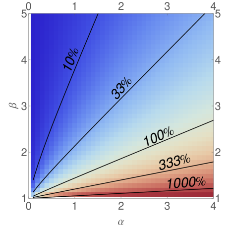
Equation (10), , represents the a-priori probability that a planet transits, given its scaled semi-major axis and accounting the effects of orbital eccentricity. This new equation has important ramifications for expected survey yields, statistical validation of planets and occurrence rate calculations. In the latter instance, many authors have previously simply assumed (Howard et al., 2012; Dong & Zhu, 2013; Dressing & Charbonneau, 2013; Petigura et al., 2013) and thus not accounted for the terms due to orbital eccentricity. For example, adopting and from Kipping (2013) indicates that is increased by versus the naive circular assumption. This in-turn means that any occurrence rate calculations assuming circularity will have overestimated the true number of planets by this factor.
In Figure 1, we illustrate the enhancement factor in the transit probability as a function of and , for which different values may be appropriate for different sub-populations.
3 Eccentricity Priors
3.1 Orbital Eccentricity
In §2, we calculated the prior probability of seeing a transit, given a specific value of the orbital eccentricity. We can reverse this conditional and ask the question what is the probability distribution of the orbital eccentricity, given that one sees transits? This question may be answered by application of Bayes’ theorem:
| (11) |
Note that all of the terms in the above have been already calculated. Specifically, is given by Equation (2), is given by Equation (4) and is given by Equation (7). Inputting these expressions reveals that all terms on the right hand side (RHS) cancel out, indicating that , where
| (12) |
The related term may be found by a similar approach, writing Bayes’ theorem as:
| (13) |
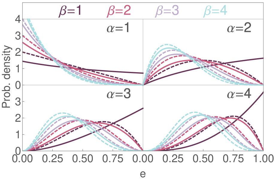
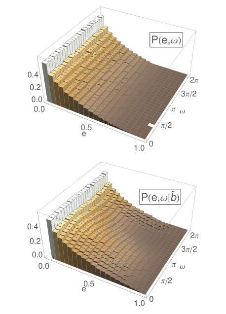
where on the second line we drop the dependence which cancels out on the RHS. We have now calculated/defined and , for which the only difference is that in the former scenario we include the conditional knowledge that the planet in question transits its host star. Figure 2 compares these two probability density functions for different realizations of and , where it is visually apparent that cases yield a significant entropy change.
Consider regressing some photometric time series and/or radial velocity time series of a planet known to transit its host star with a physical model accounting for orbital eccentricity. Choosing an informative prior in naturally and quantitively includes the observer’s prior knowledge about what a typical orbital solution looks like. For an informative prior, we advocate using rather than , which then accounts for the fact a transiting planet is a-priori more likely to be eccentric.
In general, Monte Carlo regressions may impose priors by employing inverse transform sampling (Devroye, 1986). This process allows one to generate a uniform random variate, , over the interval and transform it into a random variate drawn from any arbitrary probability distribution. This is achieved by finding the inverse of the cumulative density function (CDF). For , a closed-form solution for the CDF is tractable, but the inverse is not. However, given a closed-form solution for the CDF, one may apply Newton’s method to solve the inverse and generate samples from the target distribution. Accordingly, the iteration of is then
| (14) |
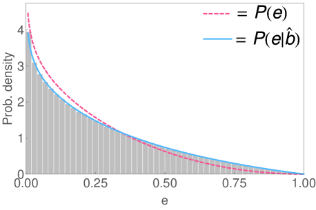
where is a random uniform variate, is the incomplete Beta function and is Appell’s hypergeometric function. In Figure 3, we show a histogram of random variates drawn from using this algorithm, assuming and . The ensemble distribution provides excellent agreement to the closed-form probability density function (PDF) of , as expected.
3.2 Argument of Periastron
In §2, we recovered the well-known result (e.g. see Barnes 2007) that the geometric probability of a planet transiting its host star is higher for planets with large orbital eccentricity (see Equations 2&6). Another well-known result for eccentric transiting planets, is that eccentric planets are most likely to transit near periapsis () than apoapsis (), since the planet makes it closest approach at this point. To our knowledge, our derived equation in Equation (7) is the first quantification of this geometric enhancement. Since periapsis transits are more likely to transit, it therefore follows that for planets known to transit, the prior distribution of should have a maximum at and a minimum at . In other words, the prior distribution of for transiting planets is manifestly non-uniform. Here, we derive this prior by application of Bayes’ theorem; specifically
| (15) |
All three terms on the RHS have been defined earlier in this work, specifically is given by Equation (7), is independent of and thus given by Equation (3) and finally was computed in Equation (10). Using these expressions, the dependence cancels out, indicating , where
| (16) |
Inverse transform sampling may be accomplished by evaluating the inverse CDF. Similar to the case with , we were able to find a closed-form solution for the CDF of , but the inverse yields a transcendental equation. Again, Newton’s method allows for a simple recursive algorithm to quickly compute the inverse and thus sample directly from the prior , via
| (17) |
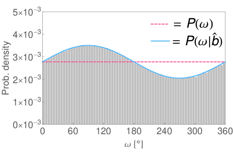
where is a random uniform variate. In Figure 4, we plot a histogram of samples drawn from , assuming and . The ensemble distribution provides excellent agreement to the closed-form PDF of , as expected.
Finally, it is worth noting that one can construct a prior for in the case where is also known, via Bayes’ theorem:
| (18) |
The terms on the RHS have been calculated/defined earlier in this work. Specifically, is given by Equation (2), is independent of and and thus given in Equation (3) and finally is given by Equation (6). Using these results, we find the dependency cancels out, indicating that , where
| (19) |
3.3 Joint Prior Probability
The priors derived thus far are for the univariate case of and . However, it is often useful to have the joint probability density function i.e. . Consider first the simple scenario of a planet where it is unknown whether it transits or not. Here, one may define such a prior using Bayes’ theorem in two equivalent ways:
| (20) |
Since is assumed to be independent of (Equation 3) and is assumed to be independent of (Equation 4), then these forms are equivalent to
| (21) |
For transiting planets, adding in the conditional probability of yields two equivalent forms
| (22) |
which evaluate to the same solution of
| (23) |
It is important to note that the joint probability distribution is not equal to simply multiplying the two independent priors, as was the case for planets not known whether they transit. Specifically, whilst it is true that , for transiting planets we have . The joint probability distribution therefore includes the conditional dependence between and (this is illustrated in Figure 5).
When comparing an observed distribution to a model distribution, it is often useful to consider the CDF rather than PDF, in order to eliminate the effects of subjectively choosing a bin size (Kipping, 2013). To this end, we here provide the closed-form solution of the joint CDF , given by
| (24) |
where we define
| (25) | ||||
| (26) |
Sampling from a multivariate joint probability probability is more elaborate than the univariate case. We first require expanding the CDF of the joint probability distribution using the product rule:
| (27) |
The relation above indicates that one may first draw an sample, , using the inverse of and then using this value as a conditional when inverting to obtain an sample, .
| (28) | ||||
| (29) |
where and are uniform random variates and and are random variates drawn from . The inverse of is computed using the recursive relation presented in Equation (14). The inverse of has not yet been found and is distinct from the inverse of , for which we presented a recursive relation earlier in Equation (17). As before, the inverse requires solving a transcendental equation and again we find that Newton’s method provides an efficient solution, using the iterations
| (30) |
We provide Fortran code, ECCSAMPLES (download link), to to draw joint samples from using the method described above. ECCSAMPLES computes using the F1 algorithm by Colavecchia & Gasaneo (2004) and requires s per sample for 1% accuracy on a hyperthreaded Intel Core i7-3720QM processor. Various special functions and dependencies required in ECCSAMPLES come from Majumder & Bhattacharjee (1973), Cran et al. (1977), Macleod (1989), Zhang & Jin (1996) and Forrey (1997). An example bivariate histogram of samples generated by this code is shown in Figure 5.
4 Discussion
4.1 Implications for Occurrence Rate Estimates
It has been previously established that eccentric planets have an enhanced probability of transiting their host star (Barnes, 2007). Specifically, one finds ; a result which we recover in Equation (6). However, in practice, the thousands of transiting planet candidates found by the Kepler Mission (Borucki et al., 2009; Batalha et al., 2013) do not have individually measured eccentricities. For this reason, calculations using the ensemble population, such as planet occurrence rate estimates, require marginalizing out the eccentricity term.
The marginalized transit probability, , has been previously discussed in Burke (2008). In order to perform this marginalization, an assumption for the prior is required. Recall that in this work, we use the Beta distribution for , due its compact yet flexible form and since it currently provides the best description of the observed eccentricity distribution (Kipping, 2013). Without the hundreds of well-measured eccentricities available by the time of Kipping (2013), Burke (2008) used a piece-wise distribution of the form
| (31) |
Using this prior with and , Burke (2008) estimate that the marginalized transit probability is enhanced by % relative to an assumption of circularity. In this work, we find that the transit probability is enhanced via Equation (10). Drawing samples of and from the posterior distributions derived in Kipping (2013), we estimate an enhancement factor of % for all planets in the Kipping (2013) sample and % for planets in the “short-period” sample ( d). In both cases, we favour a much lower overall enhancement factor than Burke (2008).
In conclusion, eccentricity enhances the transit probability by %, with the exact value depending upon the sub-population in question. One important implication of this result is with respect to planet occurrence rate calculations from transit surveys. In order to compute the occurrence rate, one must account for the fact that only planets with the correct geometry transit i.e. many more planets exist than are actually observed. We note that many recent studies of the planet occurrence rate from the Kepler Mission have implicitly assumed that all planets are on circular orbits by assuming a transit probability (Howard et al., 2012; Dong & Zhu, 2013; Dressing & Charbonneau, 2013; Petigura et al., 2013). This effectively ignores the intrinsic bias of the transit technique towards eccentric planets. It can therefore be seen that all of these afore mentioned occurrence rate calculations have overestimated the true rate by %.
As an example, Dressing & Charbonneau (2013) estimate planets per star for M-dwarfs with periods below 50 d. Using the “short-period” posterior distributions for and computed by Kipping (2013), we estimate that this occurrence rate would be modified to planets per star, which is decrease. In practice, the and values should be derived from a sample as closely matching the transit survey sample as possible. Here, the “short-period” sample of Kipping (2013) spans periods up to d, all spectral types and all detectable masses. In contrast, the Dressing & Charbonneau (2013) sample only extends up to periods of 50 d, stars cooler than 4000 K and probes down to smaller planets than that detectable by current radial velocity measurements. Querying the Exoplanet Orbit Database (Wright et al., 2011) at the time of writing, there are only 12 planets with radial velocity orbits for stars cooler than 4000 K and periods below 50 d, which is insufficient to extract a robust eccentricity distribution. This highlights the importance of measuring the eccentricity distributions in these poorly sampled parameter regions.
4.2 Implications for Extracting the Eccentricity Distribution
In §3, we derived a suite of probability distributions regarding the eccentricity of a planet, given that we know it transits. Simply put, eccentric planets are more likely to transit and thus the eccentricity distribution of transiting planets is positively biased. To our knowledge, this is the first formal demonstration of this point. We also stress that this positive bias is distinct from another positive bias in eccentricity caused by the boundary condition at (Lucy & Sweeney, 1971). However, it is worth noting that this latter bias is easily avoided by using nested sampling based regression techniques (Skilling, 2004), rather than Markov chain Monte Carlo strategies.
The fact that eccentric planets are more likely to transit means that extracting the eccentricity distribution of transiting planets requires a correction for this positive bias. Specifically, one should describe the observed distribution of transiting planet eccentricities with rather than . Recent efforts to extract the eccentricity distribution of Kepler’s planetary candidates, such as Kane et al. (2012), have not accounted for this bias and so have extracted a positively skewed distribution.
4.3 Using ECCSAMPLES to Impose Informative Priors
Two of the probability distributions derived in this work may be of use to wider community, for the purpose of serving as informative priors. Firstly, in Equation (13), we provide , which is the a-priori probability distribution of a planet’s eccentricity, given that it transits its host star. Secondly, in Equation (23), we provide , which is the a-priori joint probability distribution of a planet’s eccentricity and argument of periastron, given that it transits its host star.
These probability distributions may be used as priors when fitting any kind of data of transiting planets, for which the eccentricity is a dependent variable. This is particularly useful in cases where the data poorly constrains and , yet one wishes to fully propagate the intrinsic uncertainty in these parameters into the regression process. One example would be fitting low signal-to-noise radial velocity data of transiting systems, where the planetary mass and eccentricity exhibit strong correlations (Cumming, 2004; Ford, 2005). Another example would be fitting transit light curves of any signal-to-noise level, since transit data contains very little information on the eccentricity (Kipping, 2008).
In order to facilitate the easy adoption of such priors, we provide Fortran code, ECCSAMPLES, available via this hyperlink. ECCSAMPLES allows one to transform a uniform variate, , into a variate drawn from i.e. . In a typical Monte Carlo regression, one would explore parameter space as usual using the uniformly distributed parameters . At each realization, the likelihood (or ) calculation is made with a trial , which comes from transforming the current trial into using ECCSAMPLES. Therefore, the call to ECCSAMPLES would simply be inserted just before the likelihood call.
ECCSAMPLES can draw samples from and , as well as and for cases where it is unknown whether the planet transits. In all cases, a fundamental assumption is that is described by a Beta distribution with shape parameters and (Kipping, 2013). One may even choose to allow and to vary, which is to say one implements hyper-priors. ECCSAMPLES therefore provides an flexible tool for imposing eccentricity priors.
Acknowledgments
This work was performed [in part] under contract with the California Institute of Technology (Caltech)/Jet Propulsion Laboratory (JPL) funded by NASA through the Sagan Fellowship Program executed by the NASA Exoplanet Science Institute. This research has made use of the Exoplanet Orbit Database and the Exoplanet Data Explorer at exoplanets.org.
References
- Baglin et al. (2006) Baglin, A. et al., 2006, in The COROT Mission Pre-Launch Status, ed. M. Fridlund, A. Baglin, J. Lochard & L. Conroy, ESA SP-1306, 33–37
- Barnes (2007) Barnes, J. W., 2007, PASP, 119, 986
- Batalha et al. (2013) Batalha, N. M. et al., 2013, ApJS, 204, 24
- Beatty & Gaudi (2008) Beatty, T. G. & Gaudi, S. B., 2008, ApJ, 686, 1302
- Berta et al. (2013) Berta, Z. K., Irwin, J. & Charbonneau, D., 2013, ApJ, 775, 91
- Borucki et al. (2009) Borucki W. et al., 2009, in Pont F., Sasselov D., Holman M. J., eds, Proc. IAU Symp. 253: Transiting Planets p. 289
- Burke (2008) Burke, C. J., 2008, ApJ, 679, 1566
- Butler et al. (2006) Butler, R. P. et al., 2006, ApJ, 646, 505
- Chatterjee et al. (2008) Chatterjee, S., Ford, E. B., Matsumura, S. & Rasio, F. A., 2008, ApJ, 686, 580
- Colavecchia & Gasaneo (2004) Colavecchia, F. D. & Gasaneo, G., 2004, Computer Physics Communications, 157, 32
- Cran et al. (1977) Cran, G. W., Martin, K. J. & Thomas, G. E., 1977, Applied Statistics, 26, 111
- Cumming (2004) Cumming, A., 2004, MNRAS, 354, 1165
- Dawson & Johnson (2012) Dawson, R. I. & Johnson, J. A., 2012, ApJ, 756, 13
- Dawson et al. (2012) Dawson, R. I., Johnson, J. A., Morton, T. D., Crepp, J. R., Fabrycky, D. C., Murray-Clay, R. A. & Howard, A. W., 2012, ApJ, 761, 16
- Devroye (1986) Devroye, L., 1986, “Non-uniform Random Variate Generation”, 1st edn., New York: Springer
- Dong & Zhu (2013) Dong, S. & Zhu, Z., 2013, ApJ, 778, 53
- Dressing & Charbonneau (2013) Dressing, C. D. & Charbonneau, D., 2013, ApJ, 767, 95
- Dzigan & Zucker (2012) Dzigan, Y. & Zucker, S., 2012, ApJ, 753, 1
- Ford (2005) Ford, E. B., 2005, ApJ, 642, 505
- Forrey (1997) Forrey, R. C., 1997, J. Comp. Phys., 137, 79
- Fressin et al. (2012) Fressin, F. et al., 2012, Nature, 482, 195
- Fressin et al. (2013) Fressin, F. et al., 2013, ApJ, 766, 81
- Hartman et al. (2009) Hartman, J. D. et al., 2009, ApJ, 695, 336
- Howard et al. (2012) Howard, A. W. et al., 2012, ApJS, 201, 15
- Jurić & Tremaine (2008) Jurić, M. & Tremaine, S., 2008, ApJ, 686, 603
- Kane et al. (2012) Kane, S. R., Ciardi, D. R., Gelino, D. M. & von Braun, K., 2012, MNRAS, 425, 757
- Kipping (2008) Kipping, D. M., 2008, MNRAS, 389, 1383
- Kipping (2010) Kipping, D. M., 2010, MNRAS, 407, 301
- Kipping et al. (2012) Kipping, D. M., Dunn, W. R., Jasinski, J. M. & Manthri, V. M., 2012, MNRAS, 421, 1166
- Kipping (2013) Kipping, D. M., 2013, MNRAS, 435, 2152
- Kipping (2014) Kipping, D. M., 2014, MNRAS, 440, 2164
- Lucy & Sweeney (1971) Lucy, L. B. & Sweeney, M. A., 1971, AJ, 76, 544
- Macleod (1989) Macleod, A. J., 1989, Applied Statistics, 38, 397
- Majumder & Bhattacharjee (1973) Majumde, K. L. & Bhattacharje, G. P., 1973, Applied Statistics, 22, 409
- Morton (2012) Morton, T. D., 2012, ApJ, 761, 6
- Petigura et al. (2013) Petigura, E. A., Howard, A. W., Marcy, G. W., 2013, PNAS, 110, 19175
- Rasio & Ford (1996) Rasio, F. A. & Ford, E. B., 1996, Science, 274, 954
- Rauer et al. (2014) Rauer, H. et al., 2014, Experimental Astronomy, submitted (arXiv1310.0696)
- Ricker et al. (2010) Ricker, G. R., et al. 2010, in Bulletin of the American Astronomical Society, Vol. 42, American Astronomical Society Meeting Abstracts #215, #450.06
- Shen & Turner (2008) Shen, Y. & Turner, E. L., 2008, ApJ, 685, 553
- Skilling (2004) Skilling, J. 2004, in Fischer R., Preuss R., Toussaint U. V., eds, American Institute of Physics Conference Series Nested Sampling. pp 395–405
- Torres et al. (2004) Torres, G., Konacki, M., Sasselov, D. D. & Jha, S., 2004, ApJ, 614, 979
- Trilling (2000) Trilling, D. E., 2000, ApJ, 537, 61
- Wang & Ford (2011) Wang, J. & Ford, E. B., 2011, MNRAS, 418, 1822
- Winn (2010) Winn, J. N. 2010, arXiv:1001.2010
- Wright et al. (2011) Wright, J. T. et al., 2011, PASP, 123, 412
- Youdin (2011) Youdin, A. N., 2011, ApJ, 742, 38
- Zhang & Jin (1996) Zhang, S. J. & Jin, J. M., 1996, “Computation of Special Functions”, John Wiley, Hoboken, N. J.