ASYMPTOTIC EXPANSIONS IN FREE LIMIT THEOREMS

Abstract.

We study asymptotic expansions in free probability. In a class of classical limit theorems Edgeworth expansion can be obtained via a general approach using sequences of “influence” functions of individual random elements described by vectors of real parameters $(\varepsilon_{1},\dots,\varepsilon_{n})$, that is by a sequence of functions $h_{n}(\varepsilon_{1},\dots,\varepsilon_{n};t)$, $|\varepsilon_{j}|\leq\frac{1}{\sqrt{n}}$, $j=1,\dots,n$, $t\in A\subset\mathbb{R}$ (or $\mathbb{C}$) which are smooth, symmetric, compatible and have vanishing first derivatives at zero. In this work we expand this approach to free probability. As a sequence of functions $h_{n}(\varepsilon_{1},\dots,\varepsilon_{n};t)$ we consider a sequence of the Cauchy transforms of the sum $\sum_{j=1}^{n}\varepsilon_{j}X_{j}$, where $(X_{j})_{j=1}^{n}$ are free identically distributed random variables with nine moments. We derive Edgeworth type expansions for distributions and densities (under the additional assumption that $\mbox{supp}(X_{1})\subset[-\sqrt[3]{n},\sqrt[3]{n}]$) of the sum $\frac{1}{\sqrt{n}}\sum_{j=1}^{n}X_{j}$ within the interval $(-2,2)$.

1. Introduction

Free probability theory was initiated by Voiculescu in 1980’s as a tool for understanding free group factors. The main concept in this theory is the notion of freeness, which is a counterpart of the classical independence for non-commutative random variables.

The distribution of the sum of two free random variables is uniquely determined by the distributions of the summands and called the free convolution of the initial distributions. While classical convolutions are studied via Fourier transforms, free convolutions can be studied via Cauchy transforms. Numerous results concerning the distributional behaviour of the sum of several free random variables were proved in the recent years: Free limit theorems [13, 15], the law of large numbers [3], the Berry-Esseen inequality [5, 11], the Edgeworth expansion in the free central limit theorem [7] etc. These results parallel the classical ones. On the other hand some results in free probability theory have no counterparts in classical probability theory. For example, the so called superconvergence. This type of convergence appears in free limit theorems and is stronger then usual convergence.

The Edgeworth type expansion in free probability theory was first obtained by Chistyakov and Götze in [7]. The idea is based on the approximation of the distribution of $Y_{n}:=\frac{1}{\sqrt{n}}\sum_{j=1}^{n}X_{j}$, where $X_{j}$, $j=1,\dots,n$ are free identically distributed random variables. by the shifted free Meixner distribution, The expansion for the distribution and density of $Y_{n}$ is given at the point $x+m_{3}/\sqrt{n}$, where $m_{3}$ is the third moment of $X_{1}$.

In this paper we develop a technique which was described in [9]. This approach (see Section 4) was introduced as a tool to derive asymptotic expansions and estimates for the reminder term in a class of classical functional limit theorems in abstract spaces. It is based on Taylor expansions only and hence can be applied in free probability without additional modifications. We use this method and derive the Edgeworth expansions for distributions and densities of normalized sums $Y_{n}$.

The paper is organized as follows. In Section 2 we formulate and discuss the main results. Preliminaries are introduced in Section 3. In Section 4 we describe the general scheme. In Section 5 we apply this general scheme to free probability. Section 6 is devoted to the proofs of results. In the Appendix we provide formulations of some results of the literature, in particular a more detailed and revised version of the expansion scheme outlined in [9] for the readers convenience. The results of this paper are part of the Ph.D. thesis of the second author in 2014 at the University of Bielefeld.

2. Results

Denote by $\mathcal{M}$ the family of all Borel probability measures defined on the real line $\mathbb{R}$.

Let $X_{1},X_{2},\dots$ be free self-adjoint identically distributed random variables with distribution $\mu\in\mathcal{M}$. Denote by $m_{k}$ and $\beta_{k}$ the moments and absolute moments of $\mu$. Throughout the text we assume that $\mu$ has zero mean and unit variance. Let $\mu_{n}$ be the distribution of the normalized sum $\frac{1}{\sqrt{n}}\sum_{j=1}^{n}X_{j}$. In free probability a sequence of measures $\mu_{n}$ converges to the semicircle law $\omega$ as $n$ tends to $\infty$. Moreover, $\mu_{n}$ is absolutely continuous with respect to the Lebesgue measure for sufficiently large $n$ [16].

We denote by $p_{\mu_{n}}$ the density of $\mu_{n}$. Define the Cauchy transform of a measure $\mu$:

$$G_{\mu}(z)=\int_{\mathbb{R}}\frac{\mu(dx)}{z-x},\ \ z\in\mathbb{C}^{+},$$

where $\mathbb{C}^{+}$ denotes the upper half plane.

In [7] Chistyakov and Götze obtained a formal power expansion for the Cauchy transform of $\mu_{n}$ and the Edgeworth type expansions for $\mu_{n}$ and $p_{\mu_{n}}$. Below we review these results. Assume that $\mu$ has compact support. Denote by $U_{n}(x)$ the Chebyshev polynomial of the second kind of degree $n$, which is given by the recurrence relation:

$$U_{0}(x)=1,\ \ U_{1}(x)=2x,\ \ U_{n+1}(x)=2xU_{n}(x)-U_{n-1}(x).$$ (2.1)

The formal expansion has the form

$$G_{\mu_{n}}(z)=G_{\omega}(z)+\sum_{k=1}^{\infty}\frac{B_{k}(G_{\omega}(z))}{n^{k/2}},$$ (2.2)

where

$$B_{k}(z)=\sum_{(p,m)}c_{p,m}\frac{z^{p}}{(1/z-z)^{m}}$$ (2.3)

with real coefficients $c_{p,m}$ which depend on the free cumulants $\kappa_{3},\dots,\kappa_{k+2}$ and do not depend on $n$. The free cumulants will be defined in Section 2. The summation on the right-hand side of (2.3) is taken over a finite set of non-negative integer pairs $(p,m)$. The coefficients $c_{p,m}$ can be calculated explicitly. For the cases $k=1,2$ we have

$$B_{1}(z)=\frac{\kappa_{3}z^{3}}{1/z-z},\ \ B_{2}(z)=\frac{(\kappa_{4}-\kappa_{3}^{2})z^{4}}{1/z-z}+\kappa_{3}^{2}\left(\frac{z^{5}}{(1/z-z)^{2}}+\frac{z^{2}}{(1/z-z)^{3}}\right).$$

Let us introduce some further notations. Denote by $\beta_{q}$ the $q$th absolute moment of $\mu$, and assume that $\beta_{q}<\infty$ for some $q\geq 2$. Moreover, denote

$$a_{n}:=\frac{\kappa_{3}}{\sqrt{n}},\quad b_{n}:=\frac{\kappa_{4}-\kappa_{3}^{2}+1}{n},\quad d_{n}:=\frac{\kappa_{4}-\kappa_{3}^{2}+2}{n},\quad n\in\mathbb{N}.$$

Introduce the Lyapunov fractions

$$L_{qn}:=\frac{\beta_{q}}{n^{(q-2)/2}}\quad\mbox{and let}\quad\rho_{q}(\mu_{t}):=\int_{|x|>t}|x|^{q}\mu(dx),\ \ t>0.$$

Denote

$$q_{1}:=\min\{q,3\},\ \ q_{2}:=\min\{q,4\},\ \ q_{3}:=\min\{q,5\}.$$

For $n\in\mathbb{N}$, set

$$\eta_{qs}(n):=\inf_{0<\varepsilon\leq 10^{-1/2}}g_{qns}(\varepsilon),\ \ \mbox{where}\ \ g_{qns}(\varepsilon):=\varepsilon^{s+2-q_{s}}+\frac{\rho_{q_{s}}(\mu,\varepsilon\sqrt{n})}{\beta_{q_{s}}}\varepsilon^{-q_{s}}$$

provided that $\beta_{q}<\infty$, $q\geq s+1$, for $s=1,2,3$, respectively. It is easy to see that $0<\eta_{qs}(n)\leq 10^{1+s/2}+1$ for $s+1\leq q_{s}\leq s+2$ and $\eta_{qs}(n)\to\infty$ monotonically as $n\to\infty$ if $s+1\leq q_{s}<s+2$, and $\eta_{qs}(n)\geq 1$, $n\in\mathbb{N}$, if $q_{s}=s+2$.

By agreement the symbols $c,\ c_{1},\ c_{2},\dots$, $c(\mu),\ c_{1}(\mu),\ c_{2}(\mu),\dots$ and $c(\mu,s)$,$\ c_{1}(\mu,s)$, $\ c_{2}(\mu,s),\dots$ shall denote absolute positive constants, absolute positive constants depending on $\mu$ and absolute positive constants depending on $\mu$ and $s$ respectively.

In the expansion below we do not assume the measure $\mu$ to be of compact support. The distribution function $\mu_{n}(-\infty,x+a_{n})$ admits the expansion:

$$\mu_{n}(-\infty,x+a_{n})=\omega(-\infty,x)$$

$$+ \left(\frac{a_{n}^{2}}{2}U_{1}\left(\frac{x}{2}\right)+\frac{a_{n}}{3}\left(3-U_{2}\left(\frac{x}{2}\right)\right)-\frac{b_{n}-a_{n}^{2}-1/n}{4}U_{3}\left(\frac{x}{2}\right)\right)\!p_{\omega}(x)+\rho_{2n}(x)$$

for $x\in\mathbb{R}$, $n\in\mathbb{N}$, where

$$|\rho_{n2}(x)|\leq c\left\{\begin{array}[]{rcl}\!\!\eta_{q3}(n)L_{qn}+L_{4n}^{3/2},&4\leq q<5\\ \!\!L_{5n},&q\geq 5.\end{array}\right.$$ (2.7)

Assume that $\mu$ has compact support, then for $n\geq c_{1}(\mu)$, $p_{\mu_{n}}$ admits the expansion

$$p_{\mu_{n}}(x+a_{n}) = \left(1+\frac{d_{n}}{2}-a_{n}^{2}-\frac{1}{n}-a_{n}x-\left(b_{n}-a_{n}^{2}-\frac{1}{n}\right)x^{2}\right)p_{\omega}(E_{n}x)$$ (2.8)

$$+\ \ \frac{c\theta}{n^{3/2}\sqrt{4-(E_{n}x)^{2}}}$$

for $x\in[-2/E_{n}+h,2/E_{n}-h]$, where $E_{n}:=(1-b_{n})/\sqrt{1-d_{n}}$ and $h=\frac{c_{2}(\mu)}{n^{3/2}}$ and $|\theta|\leq 1$.

We formulate Edgeworth type expansions obtained by the general technique which is introduced in Section 3.

First, introduce for every $\delta\in(0,1/10)$ a rectangle $K$:

$$K:=\{x+iy:x\in[-2+2\delta,\ 2-2\delta],\ |y|<\delta\sqrt{\delta}\}.$$

The following corollary follows from Theorem 5.12.

Corollary 2.1.

Assume that $\mu\in\mathcal{M}$ is supported on $[-\sqrt[3]{n},\sqrt[3]{n}]$ and $\beta_{9}<\infty$. For every $\delta\in(0,1/10)$ and $n$ such that $n\geq c(\mu)\delta^{-6}$, the Cauchy transform $G_{\mu_{n}}$ has the analytic extension

$$G_{\mu_{n}}(z)=G_{\omega}(z)+l_{n}(z),\quad z\in K,$$

where $|l_{n}(z)|\leq\frac{c}{\sqrt{\delta n}}$ on $K$.

Theorem 2.2.

Assume that $\mu\in\mathcal{M}$ is supported on $[-\sqrt[3]{n},\sqrt[3]{n}]$ and $\beta_{9}<\infty$. For every $\delta\in(0,1/10)$ the extension of the Cauchy transform $G_{\mu_{n}}$ admits the expansion

$$G_{\mu_{n}}(z)=G_{\omega}(z)+\frac{\kappa_{3}G_{\omega}^{4}(z)}{(1-G_{\omega}^{2}(z))\sqrt{n}}$$

$$+ \left(\big{(}\kappa_{4}-\kappa_{3}^{2}\big{)}\frac{G^{5}_{\omega}(z)}{1-G_{\omega}^{2}(z)}+\kappa_{3}^{2}\left(\frac{G^{7}_{\omega}(z)}{(1-G^{2}_{\omega}(z))^{2}}+\frac{G^{5}_{\omega}(z)}{(1-G^{2}_{\omega}(z))^{3}}\right)\right)\frac{1}{n}$$

$$+ \left(\frac{\kappa_{5}G_{\omega}^{6}(z)}{(1-G_{\omega}^{2}(z))}-\frac{\kappa_{3}\kappa_{4}G^{8}_{\omega}(z)\left(5G_{\omega}^{2}(z)-7\right)}{\left(1-G_{\omega}^{2}(z)\right)^{3}}\right.$$

$$+ \left.\frac{\kappa_{3}^{3}G_{\omega}^{10}(z)\left(5G_{\omega}^{4}(z)-15G_{\omega}^{2}(z)+12\right)}{\left(1-G_{\omega}^{2}(z)\right)^{5}}\right)\frac{1}{n^{3/2}}+O\left(\frac{1}{n^{2}}\right)$$

for $z\in K$, $n\geq c(\mu)\delta^{-6}$.

Due to the Stieltjes inversion formula we obtain an expansion for the densities.

Corollary 2.3.

Assume that $\mu\in\mathcal{M}$ is supported on $[-\sqrt[3]{n},\sqrt[3]{n}]$ and $\beta_{9}<\infty$. For every $\delta\in(0,1/10)$ the density $p_{\mu_{n}}$ admits the expansion

$$p_{\mu_{n}}(x)=p_{\omega}(x) + \frac{\kappa_{3}\left(x^{2}-3\right)xp_{\omega}(x)}{(4-x^{2})\sqrt{n}}$$

$$- \frac{\left(\kappa_{4}\left(x^{6}-8x^{4}+18x^{2}-8\right)-\kappa_{3}^{2}\left(2x^{6}-15x^{4}+30x^{2}-10\right)\right)p_{\omega}(x)}{\left(4-x^{2}\right)^{2}n}$$

$$+ \left(\frac{\kappa_{5}(x^{4}-5x^{2}+5)x}{(4-x^{2})}+\frac{\kappa_{3}\kappa_{4}(5x^{6}-42x^{4}+105x^{2}-70)x}{(4-x^{2})^{2}}\right.$$

$$+ \left.\frac{\kappa_{3}^{3}(5x^{8}-60x^{6}+252x^{4}-420x^{2}+210)x}{(4-x^{2})^{3}}\right)\frac{p_{\omega}(x)}{n^{3/2}}+O\left(\frac{1}{n^{2}}\right)$$

for $x\in[-2+2\delta,2-2\delta]$, $n\geq c(\mu)\delta^{-6}$.

Denote by $U_{n}(x)$ the Chebyshev polynomial of the second kind of degree $n$, which is given by the recurrence relation:

$$U_{0}(x)=1,\ \ U_{1}(x)=2x,\ \ U_{n+1}(x)=2xU_{n}(x)-U_{n-1}(x).$$ (2.9)

Corollary 2.4.

Assume that $\mu\in\mathcal{M}$ with $\beta_{9}<\infty$. For every $\delta\in(0,1/10)$ the distribution $\mu_{n}$ admits the expansion

$$\mu_{n}(a,b)=\omega(a,b) + \left[-\kappa_{3}U_{2}\left(\frac{x}{2}\right)\frac{p_{\omega}(x)}{3\sqrt{n}}\right.$$

$$+ \left(-\kappa_{4}U_{3}\left(\frac{x}{2}\right)+2\kappa_{3}^{2}\left(U_{3}\left(\frac{x}{2}\right)+U_{1}\left(\frac{x}{2}\right)-\frac{U_{1}\left(\frac{x}{2}\right)}{4-x^{2}}\right)\right)\frac{p_{\omega}(x)}{4n}$$

$$+ \left(\frac{\kappa_{5}}{5}U_{4}\left(\frac{x}{2}\right)-\frac{\kappa_{3}\kappa_{4}}{4-x^{2}}\left(U_{6}\left(\frac{x}{2}\right)-U_{4}\left(\frac{x}{2}\right)\right)\right.$$

$$- \left.\left.\frac{\kappa^{3}_{3}}{3(4-x^{2})^{2}}\left(3U_{8}\left(\frac{x}{2}\right)-7U_{6}\left(\frac{x}{2}\right)+4U_{4}\left(\frac{x}{2}\right)\right)\right)\frac{p_{\omega}(x)}{n^{3/2}}\right]\Bigg{|}_{a}^{b}+O\left(\frac{1}{n^{2}}\right)$$

with $(a,b)\subset[-2+2\delta,2-2\delta]$, $n\geq c(\mu)\delta^{-6}$ and $U_{n}(x)$ are Chebychev polynomials (2.9).

Remark 2.5.

If we assume that $\beta_{k}<\infty$, $k>9$, then the above results with accuracy $O(n^{-2})$ in Theorem 2.2, Corollary 2.3 and Corollary 2.4 can be easily expanded to the higher orders using more terms of the scheme for asymptotic expansions (4.9), provided in the interval $[-2+2\delta,2-2\delta]$.

Remark 2.6.

Assume that $m_{3}=0$, then due to (2.4) we get

$$\mu_{n}(a,b)=\omega(a,b)-\left[\frac{\kappa_{4}}{4n}U_{3}\left(\frac{x}{2}\right)-\frac{\kappa_{5}}{5n^{3/2}}U_{4}\left(\frac{x}{2}\right)\right]p_{\omega}(x)\Bigg{|}_{a}^{b}+O\left(\frac{1}{n^{2}}\right)$$

with $(a,b)\subset[-2+2\delta,2-2\delta]$, $n\geq c(\mu)\delta^{-6}$.

In the example below we consider asymptotic expansions for free convolutions of the free Poisson law.

Example 2.7 (Free Poisson law).

Let us consider the free Poisson law with density

$$p_{\mu}(x)=\frac{1}{2\pi(x+1)}\sqrt{4(x+1)-(x+1)^{2}},\quad-1\leq x\leq 3,$$

which has moments $m_{1}=0$, $m_{2}=1,$ $m_{3}=1$, $m_{4}=3$, $m_{5}=6$. The density of $p_{\mu_{n}}(x)$ is given by

$$p_{\mu_{n}}(x)=\frac{\sqrt{(4n-1)+2\sqrt{n}x-nx^{2}}}{2\pi\left(\sqrt{n}+x\right)},\quad-2+n^{-1/2}\leq x\leq 2-n^{-1/2}.$$

We consider $p_{\mu_{10}}(x)$ and $p_{\mu_{100}}(x)$:

$$p_{\mu_{10}}(x)=\frac{\sqrt{39+2\sqrt{10}x-10x^{2}}}{2\pi\left(\sqrt{10}+x\right)},\quad-2+1/\sqrt{10}\leq x\leq 2+1/\sqrt{10};$$

$$p_{\mu_{100}}(x)=\frac{\sqrt{399+20x-100x^{2}}}{2\pi(10+x)},\quad-2+1/10\leq x\leq 2-1/10.$$

In Figure 1, one can see plots of the densities and the approximations of the densities based on Corollary 2.3.

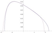
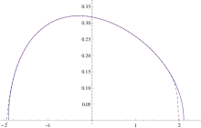
Figure 1. Comparison of the asymptotic expansion, shown as the dashed line and the exact result, shown as the solid line, $n=10$ (on the left) and $n=100$ (on the right).

3. Preliminaries

3.1. Free convolution

Let us assume that the measure $\mu\in\mathcal{M}$ has compact support contained in $[-L,L]$. Recall that the Cauchy transform is defined by

$$G_{\mu}(z)=\int_{\mathbb{R}}{\frac{\mu(dx)}{z-x}},\quad z\in\mathbb{C}^{+},$$

which is an analytic function on the upper half-plane. A measure is uniquely determined by its Cauchy transform and can be recovered from its Cauchy transform by the Stieltjes inversion formula:

$$\mu(a,b)=-\frac{1}{\pi}\lim_{y\downarrow 0}\int_{a}^{b}\Im G_{\mu}(x+iy)dx,\quad\mu(\{a\})=\mu(\{b\})=0.$$ (3.1)

Since $\mu$ is compactly supported the Cauchy transform has the following power series expansion at $z=\infty$

$$G_{\mu}(z)=\sum_{k=0}^{\infty}\frac{m_{k}}{z^{k+1}},$$ (3.2)

where $m_{k}$ are the moments of the measure $\mu$. Moreover, $|m_{k}|\leq L^{k}$. It is easy to see that $G_{\mu}(z)=\frac{1}{z}(1+o(1))$ at $z=\infty$. The series (3.2) is univalent for large $z$ ($|z|>L$) and we can define its functional inverse $K_{\mu}(z)$ such that $K_{\mu}(G_{\mu}(z))=z,$ which converges in a neighbourhood of zero. Let us introduce the function

$$R_{\mu}(z)=K_{\mu}(z)-\frac{1}{z}.$$ (3.3)

This function is called the $R$-transform and can be expressed as formal power series:

$$R_{\mu}(z)=\sum_{l=0}^{\infty}\kappa_{l+1}z^{l},$$

where the coefficients $\kappa_{k}$ are called the free cumulants of a corresponding measure. In the case when $m_{1}=0$ and $m_{2}=1$ we note that $\kappa_{1}=0$, $\kappa_{2}=1$, $\kappa_{3}=m_{3}$, $\kappa_{4}=m_{4}-2$, $\kappa_{5}=m_{5}-5m_{3}$. For cumulants of higher order the following inequalities have been established in [11]:

$$|\kappa_{l}|\leq\frac{2L}{l-1}(4L)^{l-1},\quad l\geq 2.$$ (3.4)

Next, we note some scaling properties of the Cauchy transform and the $R$-transform. We denote by $D_{t}\mu$ the dilation of a measure $\mu$ by the factor $t$:

$$D_{t}\mu(A)=\mu(t^{-1}A),\qquad(A\subset\mathbb{R}\quad\mbox{measurable}).$$

Then the Cauchy transform and the $R$-transform of the rescaled measure $D_{t}\mu$ are

$$G_{D_{t}\mu}(z)=t^{-1}G_{\mu}(t^{-1}z)\quad\mbox{and}\quad R_{D_{t}\mu}(z)=tR_{\mu}(tz).$$ (3.5)

Voiculescu in [14] proved that for two given compactly supported probability measures $\mu_{1}$ and $\mu_{2}$ the $R$-transform of the free convolution $\mu_{1}\boxplus\mu_{2}$ is given by the formula

$$R_{\mu_{1}\boxplus\mu_{2}}(z)=R_{\mu_{1}}(z)+R_{\mu_{2}}(z),$$ (3.6)

on the common domain of these functions. Moreover, (3.6) implies that the free convolution is commutative and associative.

Let us introduce the reciprocal Cauchy transform

$$F_{\mu}(z)=1/G_{\mu}(z),\quad z\in\mathbb{C}^{+},$$

which is an analytic self-mapping of $\mathbb{C^{+}}$.

Chistyakov and Götze [6], Bercovici and Belinschi [2], Belinschi [1] proved the subordination property of free convolution: there exit analytic functions $Z_{1},Z_{2}:\mathbb{C}^{+}\to\mathbb{C}^{+}$ such that

$$\lim_{y\uparrow\infty}\frac{Z_{j}(iy)}{iy}=1,\quad j=1,2.$$

Functions $Z_{1}$ and $Z_{2}$ are called subordination functions and satisfy equations:

$$z=Z_{1}(z)+Z_{2}(z)-F_{\mu_{1}}(Z_{1}(z));$$ (3.7)

$$F_{\mu_{1}\boxplus\mu_{2}}(z)=F_{\mu_{1}}(Z_{1}(z))=F_{\mu_{2}}(Z_{2}(z)).$$ (3.8)

The next result is due to Belinschi [1] (see Theorem 3.3 and Theorem 4.1).

Theorem 3.1.

Let $\mu_{1},\ \mu_{2}$ be two Borel probability measures on $\mathbb{R}$, neither of them a point mass. The following hold:

1. The subordination functions from (3.7) and (3.8) have limits $Z_{j}(x):=\lim_{y\downarrow 0}Z_{j}(x+iy),$ $j=1,2,$ $x\in\mathbb{R}.$

2. The absolutely continuous part of $\mu_{1}\boxplus\mu_{2}$ is always nonzero, and its density is analytic wherever positive and finite, and $F_{\mu_{1}\boxplus\mu_{2}}$ extends analytically in a neighbourhood of every point where the density is positive and finite.

3.2. Semicircle law.

The semicircle law plays a key role in free probability. The centered semicircle distribution of variance $t$ is denoted by $\omega_{t}$ and has the density

$$p_{\omega_{t}}(x)=\frac{1}{2\pi t}\sqrt{(4t-x^{2})_{+}},\quad x\in\mathbb{R},$$

where $a_{+}:=\max\{a,0\}$. We denote by $\omega$ the standard semicircle law that has zero mean, unit variance and the density

$$p_{\omega}(x)=\frac{1}{2\pi}\sqrt{(4-x^{2})_{+}},\quad x\in\mathbb{R}.$$

The Cauchy transform of $\omega_{t}$ is given by

$$G_{\omega_{t}}(z)=\frac{z-\sqrt{z^{2}-4t}}{2t},\qquad z\in\mathbb{C}^{+}.$$

The function $\sqrt{z^{2}-4t}$ is double-valued and has branch points at $z=\pm 2\sqrt{t}$. We can define two single-valued analytic branches on the complex plane cut along the segment $-2\sqrt{t}\leq x\leq 2\sqrt{t}$ of the real axis. Since the Cauchy transform has asymptotic behaviour $1/z$ at infinity, we can choose a branch such that $\sqrt{-1}=i$ on $\mathbb{C}^{+}$. The Cauchy transform $G_{\omega_{t}}(z)$ has a continuous extension to $\mathbb{C}^{+}\cup\mathbb{R}$ which acts on $\mathbb{R}$ by

$$\left\{\begin{array}[]{rcl}(x-i\sqrt{4t-x^{2}})/2t,\qquad\mbox{if}\ |x|\leq 2\sqrt{t};\\ (x-\sqrt{x^{2}-4t})/2t,\ \qquad\mbox{if}\ |x|>2\sqrt{t}.\\ \end{array}\right.$$ (3.11)

We see that for every $\delta>0$, the function $G_{\omega_{t}}$ can be continued analytically to the domain $K=\{x+iy:x\in(-2\sqrt{t},2\sqrt{t}),|y|<\delta\}$ and beyond to the whole Riemann surface This analytic continuation is again denoted by $G_{\omega_{t}}$. It has the explicit formula $G_{\omega_{t}}(z)=(z-i\sqrt{4t-z^{2}})/2t$, where the branch of the square root on $\mathbb{C}^{+}$ is chosen such that $\sqrt{-1}=i$. The function $G_{\omega}$ satisfies the functional equation

$$G_{\omega}(z)+F_{\omega}(z)=z,\quad z\in\mathbb{C}^{+}\cup K.$$ (3.12)

One can compute the $R$-transform of the semicircle law: $R_{\omega}(z)=z.$

3.3. Distance between two measures.

Below we recall a number of results that we need in the sequel.

We introduce the Kolmogorov (or uniform) distance between two measures $\mu$ and $\lambda$, which is defined by the formula

$$d_{K}(\mu,\lambda)=\sup_{x\in\mathbb{R}}\{|\mu((-\infty,x))-\lambda((-\infty,x))|\}.$$

and the Levy distance between two measures $\mu$ and $\lambda$ is defined by the formula

$$d_{L}(\mu,\lambda)=\inf\{s\geq 0:\mu((-\infty,x-s))-s\leq\lambda((-\infty,x))\leq\mu((-\infty,x+s))+s,\ \forall x\in\mathbb{R}\}.$$

The Levy distance is related to the Kolmogorov one by the inequality:

$$d_{L}(\mu,\lambda)\leq d_{K}(\mu,\lambda).$$

We need the following result by Voiculescu and Bercovici [4] about continuity of free convolutions with respect to the Levy and Kolmogorov distances.

Theorem 3.2.

If $\mu_{1},\ \mu_{2},\ \nu_{1},$ and $\nu_{2}\in\mathcal{M}$, then

$$d_{L}(\mu_{1}\boxplus\nu_{1},\mu_{2}\boxplus\nu_{2})\leq d_{L}(\mu_{1},\mu_{2})+d_{L}(\nu_{1},\nu_{2}),$$

$$d_{K}(\mu_{1}\boxplus\nu_{1},\mu_{2}\boxplus\nu_{2})\leq d_{K}(\mu_{1},\mu_{2})+d_{K}(\nu_{1},\nu_{2}).$$

The Berry–Esseen type inequality in free probability was proved by Chistyakov and Götze [7]. Assume $\mu$ has zero mean, unit variance and finite third absolute moment $\beta_{3}$, then there exists an absolute constant $c>0$ such that

$$d_{K}(\omega,\mu_{n})\leq\frac{c\beta_{3}}{\sqrt{n}},\quad n\in\mathbb{N}.$$ (3.13)

4. A general scheme for asymptotic expansions

We denote a vector $(\varepsilon_{1},\dots,\varepsilon_{n})\in\mathbb{R}^{n}$ by $\underline{\varepsilon}_{n}$. Let us consider a sequence of functions $h_{n}(\underline{\varepsilon}_{n};t)$, where $|\varepsilon_{j}|\leq n^{-1/2}$, $j=1,\dots,n$ and $t\in A\subseteq\mathbb{R}$ (or $\mathbb{C}$). Assume that this sequence of functions satisfies the following conditions:

$$h_{n}(\underline{\varepsilon}_{n};t)\ \mbox{is symmetric in all }\varepsilon_{j};$$ (4.1)

the sequence $h_{n}$ is compatible, which means

$$h_{n+1}(\varepsilon_{1},\dots,\varepsilon_{j-1},0,\varepsilon_{j+1},\dots\varepsilon_{n+1};t)=h_{n}(\varepsilon_{1},\dots,\varepsilon_{j-1},\varepsilon_{j+1},\dots,\varepsilon_{n+1};t),$$ (4.2)

$$\quad\quad\quad\quad\quad\quad\quad\quad\quad\quad\quad\quad\quad\quad\quad\quad\quad\quad\quad\quad j=1,\dots,n+1;\quad\quad$$

and all first derivatives vanish at zero:

$$\frac{\partial}{\partial\varepsilon_{j}}h_{n}(\underline{\varepsilon}_{n};t)\Big{|}_{\varepsilon_{j}=0}=0,\quad j=1,\dots,n.$$ (4.3)

Let us denote by $E_{m,s}^{n}$ $(m\geq n>s\geq 3)$ the set of weight vectors $\underline{\varepsilon}_{m+s}$ where all but $2s$ components are equal to $m^{-1/2}$ and the remaining $2s$ components are bounded by $n^{-1/2}$. Let $\alpha=(\alpha_{1},\dots,\alpha_{m})$ denote an $m$-dimensional multi-index. Finally, we define

$$d^{s}_{r}(h,n):=\sup\{|D^{\alpha}h_{m+s}(\underline{\varepsilon}_{m+s};t)|:|\alpha|=r,\ t\in A,\ \underline{\varepsilon}_{m+s}\in E_{m,s}^{n},\ m\geq n\}.$$

The following proposition from [9] shows that the limit

$$h_{\infty}(\underline{\varepsilon}_{s};t):=\lim_{m\rightarrow\infty}h_{m+s}(m^{-1/2},\dots,m^{-1/2},\underline{\varepsilon}_{s};t),\ \ |\varepsilon_{j}|\leq n^{-1/2},\ j=1,\dots,s$$

exists.

Proposition 4.1.

Assume $h_{m+s}(\underline{\varepsilon}_{m+s};t)$, $\underline{\varepsilon}_{m+s}\in E_{m,s}^{n}$, $m\geq n\geq s\geq 3$, $t\in A$ satisfies conditions $(\ref{sym})-(\ref{fd})$ and the condition $d^{s}_{3}(h,n)<\infty.$ Then limit $h_{\infty}(\underline{\varepsilon}_{s};t)$, $|\varepsilon_{j}|\leq n^{-1/2}$, $j=1,\dots,s$ exists and the following estimate holds:

$$|h_{n+s}(n^{-1/2},\dots,n^{-1/2},\underline{\varepsilon}_{s};t)-h_{\infty}(\underline{\varepsilon}_{s};t)|\leq cd^{s}_{3}(h,n)n^{-1/2},$$

where $c$ is an absolute constant.

We formulate an Edgeworth type expansion for $h_{n}(n^{-1/2},\dots,n^{-1/2};t)$ in terms of derivatives of $h_{\infty}(\underline{\varepsilon}_{s};t)$ with respect to $\varepsilon_{j}$, $j=1,\dots,s$ at $\underline{\varepsilon}_{s}=0$. Below we introduce all necessary notations.

We establish “cumulant” differential operators $\kappa_{p}(D)$ via the formal identity

$$\sum_{p=2}^{\infty}p!^{-1}\varepsilon^{p}\kappa_{p}(D)=\ln\left(1+\sum_{p=2}^{\infty}p!^{-1}\varepsilon^{p}D^{p}\right).$$ (4.4)

Expanding in formal power series in the formal variable $\varepsilon$ on the right-hand side of this identity we obtain the definition of the cumulant operators $\kappa_{p}(D)$. Here $D^{p}$ denotes $p$-fold differentiation with respect to a single variable $\varepsilon$, and $D^{p_{1}}\cdots D^{p_{r}}=D^{(p_{1},\dots,p_{r})}$ denotes differentiation with respect to $r$ different variables $\varepsilon_{1},\dots,\varepsilon_{r}$ at the point $\underline{\varepsilon}_{r}=0$. Since the operators are applied to symmetric functions at zero, $\kappa_{p}(D)$ is unambiguously defined by $(\ref{ln})$. The first cumulant operators are $\kappa_{2}(D)=D^{2},\ \kappa_{3}(D)=D^{3},\ \kappa_{4}(D)=D^{4}-3D^{2}D^{2},$ etc.

Then, we define Edgeworth polynomial operators $P_{r}(\kappa_{.}(D))$ by means of the following formal series in $\kappa_{r}$ and a formal variable $\varepsilon$.

$$\sum_{r=0}^{\infty}\varepsilon^{r}P_{r}({\kappa_{.}})=\exp\left(\sum_{r=3}^{\infty}r!^{-1}\varepsilon^{r-2}\kappa_{r}\right)$$ (4.5)

which yields

$$P_{r}({\kappa_{.}})=\sum_{m=1}^{r}m!^{-1}\left\{\sum_{(j_{1},\dots j_{m})}(j_{1}+2)!^{-1}\kappa_{j_{1}+2}\cdots(j_{m}+2)!^{-1}\kappa_{j_{m}+2}\right\},$$ (4.6)

where the sum $\sum_{(j_{1},\dots,j_{m})}$ means summation over all $m$-tuples of positive integers $(j_{1},\dots,j_{m})$ satisfying $\sum_{q=1}^{m}j_{q}=r$ and ${\kappa_{.}}=(\kappa_{3},\dots,\kappa_{r+2})$. Replacing the variables $\kappa_{.}$ in $P_{r}(\cdot)$ by the differential operators

$$\kappa_{.}(D):=(\kappa_{3}(D),\dots,\kappa_{r+2}(D))$$

we obtain “Edgeworth” differential operators, say $P_{r}(\kappa_{.}(D))$. The following theorem yields an asymptotic expansion for $h_{n}(n^{-1/2},\dots,n^{-1/2};t)$ (for more details see [9]).

Theorem 4.2.

Assume that $h_{m+s}(\underline{\varepsilon}_{m+s};t)$, $\underline{\varepsilon}_{m+s}\in E_{m,s}^{n}$, $m\geq n\geq s\geq 3$, $t\in A$ fulfils conditions $(\ref{sym})-(\ref{fd})$ together with

$$d_{s}^{s}(h,n)\leq B,$$ (4.7)

$$\sup_{t\in A}\sup_{\underline{\varepsilon}_{m+s}\in E_{m,s}^{n}}\left|D^{\alpha}h_{m+s}(\underline{\varepsilon}_{m+s};t)\right|\leq B,$$ (4.8)

where $\alpha=(\alpha_{1},\dots,\alpha_{s-2})$ such that

$$\alpha_{i}\geq 2,\ \ i=1,\dots,s-2,\ \ \sum_{i=1}^{s-2}(\alpha_{i}-2)\leq s-2.$$

Then

$$\left|h_{n}(n^{-1/2},\dots,n^{-1/2};t)-\sum_{r=0}^{s-3}n^{-r/2}P_{r}(\kappa_{.}(D))h_{\infty}(\underline{\varepsilon}_{r};t)\Big{|}_{{\underline{\varepsilon}_{r}}=0}\right|\leq c_{s}Bn^{-(s-2)/2},$$ (4.9)

where $P_{0}(\kappa_{.}(D))=1$ and $P_{r}(\kappa_{.}(D))$ are given explicitly in $(\ref{ppp})$, $c_{s}$ is an absolute constant.

The first four terms of the expansion (4.9) are

$$h_{n}(n^{-1/2},\dots,n^{-1/2};t)$$

$$\!\!= h_{\infty}(0;t)+\frac{1}{n^{1/2}}\left(\frac{1}{6}\frac{\partial^{3}}{\partial\varepsilon_{1}^{3}}\right)h_{\infty}(\varepsilon_{1};t)\Big{|}_{\varepsilon_{1}=0}$$

$$\!\!+ \frac{1}{n}\left(\frac{1}{24}\left(\frac{\partial^{4}}{\partial\varepsilon_{1}^{4}}-3\frac{\partial^{2}}{\partial\varepsilon_{1}^{2}}\frac{\partial^{2}}{\partial\varepsilon_{2}^{2}}\right)+\frac{1}{72}\frac{\partial^{3}}{\partial\varepsilon_{1}^{3}}\frac{\partial^{3}}{\partial\varepsilon_{2}^{3}}\right)h_{\infty}(\underline{\varepsilon}_{2};t)\Big{|}_{\underline{\varepsilon}_{2}=0}$$

$$\!\!+ \frac{1}{48n^{3/2}}\left(\frac{1}{5}\left(\frac{\partial^{5}}{\partial\varepsilon_{1}^{5}}-10\frac{\partial^{3}}{\partial\varepsilon_{1}^{3}}\frac{\partial^{2}}{\partial\varepsilon_{2}^{2}}\right)\right.$$

$$\!\!+ \frac{1}{3}\left(\frac{\partial^{4}}{\partial\varepsilon_{1}^{4}}-3\frac{\partial^{2}}{\partial\varepsilon_{1}^{2}}\frac{\partial^{2}}{\partial\varepsilon_{2}^{2}}\right)\!\frac{\partial^{3}}{\partial\varepsilon_{3}^{3}}+\left.\frac{1}{27}\frac{\partial^{3}}{\partial\varepsilon_{1}^{3}}\frac{\partial^{3}}{\partial\varepsilon_{2}^{3}}\frac{\partial^{3}}{\partial\varepsilon_{3}^{3}}\right)h_{\infty}(\underline{\varepsilon}_{3};t)\Big{|}_{\underline{\varepsilon}_{3}=0}\!+O\left(\frac{1}{n^{2}}\right)\!.$$

Remark 4.3.

Conditions (4.7) and (4.8) guarantee that the functions

$$g^{\alpha}_{m+s}(\underline{\varepsilon}_{m+s};t):=D^{\alpha}h_{m+s}(\underline{\varepsilon}_{m+s};t),$$

for $\alpha=(\alpha_{1},\dots,\alpha_{r})$, where $r\leq s-3,\ s\geq 3$

$$\alpha_{i}\geq 2,\quad i=1,\dots,r,\quad\sum_{i=1}^{r}(\alpha_{i}-2)=s-3$$

satisfy the conditions of Proposition 4.1. In particular, due to Proposition 4.1 for every $\alpha$ the functions $g^{\alpha}_{m+s}(\underline{\varepsilon}_{m+s};t)$ converge to $g^{\alpha}_{s}(\underline{\varepsilon}_{s};t)$ as $m\to\infty$ uniformly in $\underline{\varepsilon}_{s}$, $|\varepsilon_{j}|\leq n^{-1/2}$, $n\geq 1$, $j=1,\dots,s$ and due to Theorem A.1 (see Appendix) we conclude that $g^{\alpha}_{s}(\underline{\varepsilon}_{s};t)=D^{\alpha}h_{\infty}(\underline{\varepsilon}_{s};t)$, $r\leq s-3$.

5. Proofs of results

5.1. Truncation

We assume that $\mu\in\mathcal{M}$ satisfies $\beta_{9}<\infty$. Consider free random variables $\hat{X}_{1},\hat{X}_{2},\dots$ with distribution $\hat{\mu}\in\mathcal{M}$ such that $\hat{\mu}([-n^{1/3},n^{1/3}])=1$ and $\hat{\mu}(B)=\mu(B)$ for all Borel sets $B\subseteq[-n^{1/3},n^{1/3}]\backslash\{0\}$. Denote by $\hat{\mu}_{n}$ the distribution of the random variable $\hat{Y}_{n}:=(\hat{X}_{1}+\dots+\hat{X}_{n})/\sqrt{n}$. We denote by $\hat{m}_{k}$ and $\hat{\beta}_{k}$, $k=1,2,\dots$ moments and absolute moments of $\hat{\mu}$. Let us also introduce the centered random variables

$$X^{*}_{1}:=\frac{\hat{X}_{1}-a_{n}}{b_{n}},\quad X^{*}_{2}:=\frac{\hat{X}_{2}-a_{n}}{b_{n}},\quad\dots\quad\mbox{and}\quad Y^{*}_{n}:=\frac{1}{\sqrt{n}}\sum_{j=1}^{n}X^{*}_{j},$$

where

$$a_{n}:=\hat{m}_{1},\quad b^{2}_{n}:=\int(x-a_{n})^{2}\hat{\mu}(dx)=1-\int_{A_{n}}x^{2}\mu(dx)-a_{n}^{2},\ \ A_{n}:=\{|x|>n^{1/3}\}.$$

Denote by $\mu^{*}$ and $\mu_{n}^{*}$ the distributions of the random variables $X_{1}^{*}$ and $Y_{n}^{*}$ respectively, and by $m_{k}^{*}$ and $\beta_{k}^{*}$, $k=1,2,\dots$ moments and absolute moments of $\mu^{*}$. Note that $m_{1}^{*}=0$ and $m_{2}^{*}=1$. Due to the assumption $\beta_{9}<\infty$ we have

$$|a_{n}|\leq n^{-8/3}\int_{A_{n}}|x|^{9}\mu(dx)\leq\beta_{9}n^{-8/3}$$

and

$$|1-b_{n}^{2}|\leq\beta_{9}^{2}n^{-16/3}+\beta_{9}n^{-8/3}.$$

By above inequalities we obtain

$$b_{n}^{-1}(n^{1/3}+|a_{n}|)\leq n^{1/3}.$$ (5.1)

By (5.1) we conclude that the support of $\mu^{*}$ is contained in $[-n^{1/3},n^{1/3}]$.

Furthermore, we deduce that

$$\beta^{*}_{3}\leq b_{n}^{-3}\left(\hat{\beta}_{3}+3|a_{n}|\hat{\beta}_{2}+3|a_{n}|^{2}\hat{\beta}_{1}+|a_{n}|^{3}\right)\leq b_{n}^{-3}\hat{\beta}_{3}+4\beta_{9}n^{-8/3}.$$

Let $\hat{\omega}$ be a semi-circle distribution with mean $\sqrt{n}a_{n}$ and variance $b^{2}_{n}$. By the triangle inequality we get

$$d_{K}(\mu_{n},\omega)\leq d_{K}(\mu_{n},\hat{\mu}_{n})+d_{K}(\hat{\mu}_{n},\hat{\omega})+d_{K}(\hat{\omega},\omega).$$ (5.2)

By Theorem 3.2 the first term in the right hand side has a bound

$$d_{K}(\mu_{n},\hat{\mu}_{n})\leq n\mu(\{|x|>\sqrt[3]{n}\}\leq\frac{\beta_{9}}{n^{2}}.$$ (5.3)

We find the an estimate for the last term in (5.2)

$$d_{K}(\hat{\omega},\omega)\leq c\left(\frac{1}{b_{n}}+\frac{\sqrt{n}a_{n}}{b_{n}}-1\right)\leq\frac{c}{n^{2}}.$$ (5.4)

Note, that we have an equality

$$d_{K}(\hat{\mu}_{n},\hat{\omega})=d_{K}(\mu_{n}^{*},\omega).$$

Our next aim is to apply the general asymptotic scheme for expansion to $\mu^{*}_{n}$.

5.2. Application of the general scheme for asymptotic expansions

Below we apply the general scheme to compute the asymptotic expansions for $p_{\mu^{*}_{n}}$ and $\mu_{n}$. We set $h_{n}(n^{-1/2},\dots,n^{-1/2};z):=G_{\mu^{*}_{n}}(z)$, $z\in K$, where $G_{\mu^{*}_{n}}(z)$ is the extension defined in Corollary 2.1 (in our case $\mu^{*}=\mu$). Let us introduce two notations:

$$\tilde{\mu}_{m+s} := D_{\varepsilon_{1}}\mu^{*}\boxplus\dots\boxplus D_{\varepsilon_{m+s}}\mu^{*},\quad\underline{\varepsilon}_{m+s}\in E_{m,s}^{n},\ \ m\geq n,$$

$$\mu_{s}^{(\underline{\varepsilon}_{s})} := D_{\varepsilon_{1}}\mu^{*}\boxplus\dots\boxplus D_{\varepsilon_{s}}\mu^{*},\quad|\varepsilon_{j}|\leq n^{-1/2},\quad j=1,\dots,s.$$

The following results follow from Theorem 5.12 and allow for an easy application of the expansion scheme.

Corollary 5.1.

For every $\delta\in(0,1/10)$ and $n\geq c(\mu^{*},s)\delta^{-6}$ the Cauchy transform $G_{\omega\boxplus\mu_{s}^{(\underline{\varepsilon}_{s})}}$ has an analytic continuation to $K$ such that

$$G_{\omega\boxplus\mu_{s}^{(\underline{\varepsilon}_{s})}}(z)=G_{\omega}(z)+l_{\underline{\varepsilon}_{s}}(z),\ \ z\in K,$$ (5.5)

where $|l_{\underline{\varepsilon}_{s}}(z)|\leq\frac{c(s)}{n\sqrt{\delta}}$ on $K$.

Remark 5.2.

In (5.5) we understand $G_{\omega}(z)$ as an analytic continuation of the corresponding Cauchy transform, which is defined in the following way:

$$G_{\omega}(z)=(z-i\sqrt{4-z^{2}})/2,\ \ z\in K.$$

Corollary 5.3.

For every $\delta\in(0,1/10)$ and $m\geq n\geq c(\mu^{*},s)\delta^{-6}$ the Cauchy transform $G_{\tilde{\mu}_{m+s}}$ has an analytic continuation to $K$ such that

$$G_{\tilde{\mu}_{m+s}}(z)=G_{\omega\boxplus\mu_{s}^{(\underline{\varepsilon}_{s})}}(z)+l(z),\quad z\in K,$$ (5.6)

where $|l(z)|\leq\frac{c(s)}{\sqrt{\delta n}}$ on $K$.

Corollary 5.4.

For every $\delta\in(0,1/10)$, $m\geq n\geq c(\mu^{*},s)\delta^{-6}$ the analytic continuation $G_{\tilde{\mu}_{m+s}}(z)$, $z\in K$ is a symmetric and compatible function of $\varepsilon_{j}$, $j=1,\dots,m+s$.

Theorem 5.5.

For every $\delta\in(0,1/10)$, $m\geq n\geq c(\mu^{*},s)\delta^{-6}$ the analytic continuation of $G_{\tilde{\mu}_{m+s}}(z)$, $z\in K$ is a smoothly differentiable function of variables $\varepsilon_{j}$, $j=1,\dots,2s$. (Here we mean those $2s$ variables which are not fixed and just bounded by $n^{-1/2}$). Moreover, the inequality holds:

$$\sup_{z\in K}\sup_{\underline{\varepsilon}_{m+s}\in E_{m,s}^{n}}\left|D^{\alpha}G_{\tilde{\mu}_{m+s}}(z)\right|\leq c,\quad|\alpha|\leq s.$$

Theorem 5.6.

For every $\delta\in(0,1/10)$, $m\geq n\geq c(\mu^{*},s)\delta^{-6}$ and $z\in K$

$$\frac{\partial}{\partial\varepsilon_{j}}G_{\tilde{\mu}_{m+s}}(z)\Big{|}_{\varepsilon_{j}=0}=0,\quad j=1,\dots,2s.$$

In view of the above results, we can choose the sequence of extensions of the Cauchy transforms $G_{\tilde{\mu}_{m+s}}(z)$, $z\in K$ as the sequence of functionals $h_{m+s}(\underline{\varepsilon}_{m+s};z)$, i.e.

$$h_{m+s}(\underline{\varepsilon}_{m+s};z):=G_{\tilde{\mu}_{m+s}}(z),\ \ z\in K,\ \ m\geq n\geq c(\mu^{*},s)\delta^{-6},$$

and

$$h_{\infty}(\underline{\varepsilon}_{s};z):=G_{\omega\boxplus\mu_{s}^{(\underline{\varepsilon}_{s})}}(z),\ \ z\in K,\ \ n\geq c(\mu^{*},s)\delta^{-6}.$$

Now we can apply the general scheme and compute the expansion for $G_{\mu^{*}_{n}}$ in terms of derivatives of $G_{\omega\boxplus\mu_{s}^{(\underline{\varepsilon}_{s})}}$ with respect to $\varepsilon_{j}$, $j=1,\dots,s$ at $\underline{\varepsilon}_{s}=0$.

5.3. Positivity of the density of $\tilde{\mu}_{m+s}$.

Our aim is to find an interval where the density of $\tilde{\mu}_{m+s}$ is positive. The main idea is based on the Newton-Kantorovich Theorem (see Theorem A.2, for a proof see [10]).

Let us consider a pair of measures $\nu_{1}$ and $\nu_{2}$. We can rewrite the equations (3.7) and (3.8) as a system

$$\left\{\begin{array}[]{rcl}(z-Z_{1}(z)-Z_{2}(z))^{-1}+G_{\nu_{1}}(Z_{1}(z))=0\\ (z-Z_{1}(z)-Z_{2}(z))^{-1}+G_{\nu_{2}}(Z_{2}(z))=0,\\ \end{array}\right.$$ (5.9)

where $G_{\nu_{1}}$ and $G_{\nu_{2}}$ are the Cauchy transforms of $\nu_{1}$ and $\nu_{2}$, correspondingly. Choose another pair of measures $\mu_{1}$ and $\mu_{2}$ such that the Levy distance between $\nu_{j}$ and $\mu_{j}$ is sufficiently small for $j=1,2$. Then we can define subordination functions for the couple $(\mu_{1},\mu_{2})$ as a solution of (5.9), where $G_{\nu_{1}}$ and $G_{\nu_{2}}$ are replaced by the Cauchy transforms of $\mu_{1}$ and $\mu_{2}$ correspondingly. Denote these subordination functions by $t^{0}_{1}$ and $t^{0}_{2}$. According to the Newton-Kantorovich Theorem one can show that the subordination functions $Z_{j}$ and $t^{0}_{j}$, $j=1,2$ are sufficiently close to each other. We can choose $\mu_{1}$ and $\mu_{2}$ to be equal, so that $t^{0}_{1}=t^{0}_{2}$. Such a choice essentially simplifies the structure of equations (3.7) and (3.8).

Let us prove one result about the Levy distance.

Lemma 5.7.

Assume that $\mu,\ \nu\in\mathcal{M}$ and $\mu$ has zero mean and unit variance. Then $d_{L}(\nu,\nu\boxplus\mu_{s}^{(\underline{\varepsilon}_{s})})\leq 2sn^{-1/3}$, $|\varepsilon_{j}|\leq 1/\sqrt{n}$, $j=1,\dots,k$.

Proof.

From Theorem 3.2, we get

$$d_{L}(\nu,\nu\boxplus\mu_{s}^{(\underline{\varepsilon}_{s})})\leq d_{L}(\delta_{0},\mu_{s}^{(\underline{\varepsilon}_{s})})\leq\sum_{i=1}^{s}d_{L}(\delta_{0},D_{\varepsilon_{i}}\mu),$$

where $\delta_{0}$ is a delta function. By the Chebyshev inequality we obtain

$$d_{L}(\delta_{0},D_{\varepsilon_{i}}\mu)\leq 2\varepsilon_{j}^{2/3}\leq 2n^{-1/3}.$$

Hence, $d_{L}(\nu,\nu\boxplus\mu_{s}^{(\underline{\varepsilon}_{s})})\leq 2sn^{-1/3}.$ ∎

In the sequel we need the following estimates for $G_{\omega}$.

Lemma 5.8.

For every $\delta\in(0,1/10)$ we define the set

$$K_{\delta}=\{x+iy:x\in[-2+\delta,\ 2-\delta],|y|\leq 2\delta\sqrt{\delta}\}.$$

Then, we have $G_{\omega}(K_{\delta})\subset D_{\theta,1.4}=\{z\in\mathbb{C}^{-}:\mbox{arg}\ z\in(-\pi+\theta,-\theta);|z|<1.4\},$ where the angle $\theta=\theta(\delta)$ is chosen in such a way that $2\sin\theta=\sqrt{\frac{\delta}{4}\left(1-\frac{\delta}{4}\right)}.$

Proof.

Figure 2 illustrates the sets $K_{\delta}$ and $D_{\theta,1.4}$.

Figure 2.

First we show that $G_{\omega}(K_{\delta})\subseteq D_{\theta,1.4}$, where $G_{\omega}$ is an analytic extension of the Cauchy transform of $\omega$ on $K_{\delta}$. Fix a point $z_{0}\in K_{\delta}$, and write $G_{\omega}(z_{0})=Re^{i\psi}$. In order to prove $G_{\omega}(z_{0})\in D_{\theta,1.4}$ we need to verify that $|\sin\psi|>\sin\theta$ and $R<1.4$. From the functional equation (3.12) we have

$$\left(R+\frac{1}{R}\right)\cos\psi+i\left(R-\frac{1}{R}\right)\sin\psi=z_{0}.$$

From $|\Re z_{0}|\leq 2-\delta$, we get $2|\cos\psi|\leq\left(R+\frac{1}{R}\right)|\cos\psi|\leq 2-\delta.$ This implies $|\cos\psi|\leq 1-\delta/2,$ hence

$$|\sin\psi| = \sqrt{1-\cos^{2}\psi}\geq\sqrt{1-\left(1-\delta/2\right)^{2}}=\sqrt{\delta/4\left(1-\delta/4\right)}>\sin\theta.$$

Thus we obtain the desired result $|\sin\psi|>\sin\theta$.

In order to estimate $R$ we consider the imaginary part of $z_{0}$

$$2\delta\sqrt{\delta}>|\Im z_{0}|=|\sin\psi|\left|R-\frac{1}{R}\right|>\frac{|R^{2}-1|}{R}{\frac{\sqrt{\delta}}{2}}.$$

If $R>1$, we get the inequality $R^{2}-4\delta R-1<0$. Therefore, $R$ must be bounded from above by the intercept of the positive $x$-axis and the parabola $y=R^{2}-4\delta R-1.$ The roots of the equation $R^{2}-4\delta R-1=0$ are

$$R=2\delta\pm\sqrt{4\delta^{2}+1}.$$

By the choice of $\delta$ we have $2\delta+\sqrt{4\delta^{2}+1}<1.22$. This implies $R<1.4.$ ∎

The following inequalities are due to Kargin [12].

Lemma 5.9.

Let $d_{L}(\mu_{1},\mu_{2})\leq p$ and $z=x+iy$, where $y>0$. Then

1. $|G_{\mu_{1}}(z)-G_{\mu_{2}}(z)|<\widetilde{c}py^{-1}\max\{1,\ y^{-1}\}$, where $\widetilde{c}>0$ is a numerical constant;

2. $|\frac{d^{r}}{dz^{r}}(G_{\mu_{2}}(z)-G_{\mu_{1}}(z))|<\widetilde{c}_{r}py^{-1-r}\max\{1,\ y^{-1}\}$, where $\widetilde{c}_{r}>0$ are numerical constants.

Consider a pair of measures $(\nu_{1},\nu_{2})$ and introduce a function $F(t):\mathbb{C}^{2}\to\mathbb{C}^{2}$ by the formula

$$F(t)=\left(\begin{array}[]{c}(z-t_{1}-t_{2})^{-1}+G_{\nu_{1}}(t_{1})\\ (z-t_{1}-t_{2})^{-1}+G_{\nu_{2}}(t_{2})\end{array}\right).$$

The equation $F(t)=0$ has a unique solution, say $Z=(Z_{1}(z),Z_{2}(z))$, where $Z_{1}(z)$ and $Z_{2}(z)$ are subordination functions. Let $(\mu_{1},\mu_{2})$ be another pair of measures. Assume $t^{0}=(t^{0}_{1},t^{0}_{2})=(t^{0}_{1}(z),t^{0}_{2}(z))$ solves the system of equations

$$\left\{\begin{array}[]{rcl}(z-t^{0}_{1}-t^{0}_{2})^{-1}+G_{\mu_{1}}(t^{0}_{1})=0\\ (z-t^{0}_{1}-t^{0}_{2})^{-1}+G_{\mu_{2}}(t^{0}_{2})=0.\\ \end{array}\right.$$

Then $F(t^{0})$ has the form

$$F(t^{0})=\left(\begin{array}[]{cc}G_{\nu_{1}}(t^{0}_{1})-G_{\mu_{1}}(t^{0}_{1})\\ G_{\nu_{2}}(t^{0}_{2})-G_{\mu_{2}}(t^{0}_{2})\end{array}\right).$$

The derivative of $F$ with respect to $t$ at $t^{0}$ is

$$F^{\prime}(t^{0})=\left(\begin{array}[]{cc}G^{\prime}_{\nu_{1}}(t^{0}_{1})+G^{2}_{\mu_{1}}(t^{0}_{1})&G^{2}_{\mu_{1}}(t^{0}_{1})\\ G^{2}_{\mu_{2}}(t^{0}_{2})&G^{\prime}_{\nu_{2}}(t^{0}_{2})+G^{2}_{\mu_{2}}(t^{0}_{2})\end{array}\right).$$

The inverse matrix of $F^{\prime}(t^{0})$ is

$$[F^{\prime}(t^{0})]^{-1}=\frac{1}{\det[F^{\prime}(t^{0})]}\left(\begin{array}[]{cc}G^{\prime}_{\nu_{2}}(t^{0}_{2})+G^{2}_{\mu_{2}}(t^{0}_{2})&-G^{2}_{\mu_{1}}(t^{0}_{1})\\ -G^{2}_{\mu_{2}}(t^{0}_{2})&G^{\prime}_{\nu_{1}}(t^{0}_{1})+G^{2}_{\mu_{1}}(t^{0}_{1})\end{array}\right),$$ (5.15)

where

$$\det[F^{\prime}(t^{0})]=(G^{\prime}_{\nu_{2}}(t^{0}_{2})+G^{2}_{\mu_{2}}(t^{0}_{2}))(G^{\prime}_{\nu_{1}}(t^{0}_{1})+G^{2}_{\mu_{1}}(t^{0}_{1}))-G^{2}_{\mu_{1}}(t^{0}_{1})G^{2}_{\mu_{2}}(t^{0}_{2}).$$

After simple computations, we obtain

$$[F^{\prime}(t^{0})]^{-1}F(t^{0})=\frac{1}{\det[F^{\prime}(t^{0})]}\left(\begin{array}[]{c}(G^{\prime}_{\nu_{2}}(t^{0}_{2})+G^{2}_{\mu_{2}}(t^{0}_{2}))S_{1}(t^{0}_{1})-G^{2}_{\mu_{1}}(t^{0}_{1})S_{2}(t^{0}_{2})\\ (G^{\prime}_{\nu_{1}}(t^{0}_{1})+G^{2}_{\mu_{1}}(t^{0}_{1}))S_{2}(t^{0}_{2})-G^{2}_{\mu_{2}}(t^{0}_{2})S_{1}(t^{0}_{1})\end{array}\right),$$ (5.18)

where $S_{j}(t^{0}_{j}):=G_{\nu_{j}}(t^{0}_{j})-G_{\mu_{j}}(t^{0}_{j})$.

The second derivative of $F$ with respect to $t$ at $t_{0}$ is

$$F^{\prime\prime}(t^{0})=\left(\begin{array}[]{cccc}D_{1}(t^{0}_{1})&2G^{3}_{\mu_{2}}(t^{0}_{2})&2G^{3}_{\mu_{1}}(t^{0}_{1})&2G^{3}_{\mu_{2}}(t^{0}_{2})\\ 2G^{3}_{\mu_{1}}(t^{0}_{1})&2G^{3}_{\mu_{2}}(t^{0}_{2})&2G^{3}_{\mu_{1}}(t^{0}_{1})&D_{2}(t^{0}_{2})\end{array}\right),$$ (5.21)

where $D_{j}(t^{0}_{j}):=G^{\prime\prime}_{\nu_{j}}(t^{0}_{j})-2G^{3}_{\mu_{j}}(t^{0}_{j})$.

Proposition 5.10.

Let $\nu_{1},\nu_{2}\in\mathcal{M}$ be measures neither of them being a point mass. Then for every $\delta\in(0,1/10)$ there exists $c$ such that if $d_{L}(\omega,\nu_{1}\boxplus\nu_{2})\leq c\delta^{2}$ then the density $p_{\nu_{1}\boxplus\nu_{2}}(x)$ is positive and analytic on $[-2+\delta,2-\delta]$.

Proof.

We would like to find an interval where the density is positive. To this end, define a subordination function $Z_{\omega_{1/2}}(z)$ which solves the equations

$$z=2Z_{\omega_{1/2}}(z)-F_{\omega_{1/2}}(Z_{\omega_{1/2}}(z))\quad\mbox{and}\quad F_{\omega}(z)=F_{\omega_{1/2}}(Z_{\omega_{1/2}}(z)).$$

Solving this equations obtaining we obtain

$$Z_{\omega_{1/2}}(z)=\frac{3z+\sqrt{z^{2}-4}}{4},$$

and an analytic continuation of $Z_{\omega_{1/2}}$ to $K_{\delta}$ is given by

$$Z_{\omega_{1/2}}(z)=\frac{3z+i\sqrt{4-z^{2}}}{4}.$$

It easy to see that the following inequality holds:

$$\Im Z_{\omega_{1/2}}(x)>\sqrt{\delta}/3,\quad x\in[-2+\delta,2-\delta].$$

On $\mathbb{C}^{2}$ we choose the norm:

$$\|(z_{1},z_{2})\|=\sqrt{|z_{1}|^{2}+|z_{2}|^{2}}.$$

Now we apply the Newton-Kantorovich Theorem (see Theorem A.2) to the equation $F(t)=0$ for $z\in M:=\{x+iy:x\in[-2+\delta,2-\delta],\ 0<y<\delta\sqrt{\delta}\}$. In formulas (5.15), (5.18) and (5.21) we set $\mu_{1}=\mu_{2}=\omega_{1/2}$ and $t_{1}^{0}=t_{2}^{0}=Z_{\omega_{1/2}}$. Since $|Z_{\omega_{1/2}}(z)|<2$, $z\in M$, we choose the branch of $G_{\omega_{1/2}}$ such that $G_{\omega_{1/2}}(z)=z-i\sqrt{2-z^{2}},$ $|z|<2$.

1. First, we estimate $\|[F^{\prime}(t^{0})]^{-1}\|$. We computed $\det[F^{\prime}(t^{0})]$ above. Moreover, due to Lemma 5.9 with $p:=c\delta^{2}$ we have $G^{\prime}_{\nu_{j}}(t^{0}_{j})=G^{\prime}_{\omega_{1/2}}(t^{0}_{j})+f_{j}(t^{0}_{j})$, where $|f_{j}(t_{j}^{0})|\leq\tilde{c}_{1}p\delta^{-3/2}$ on $M$, $j=1,2$. Hence,

$$\det[F^{\prime}(t^{0})]$$

$$\!\!= \!\!\!(G^{2}_{\omega_{1/2}}(t^{0}_{2})+G^{\prime}_{\omega_{1/2}}(t^{0}_{2})+f_{2}(t_{2}^{0}))(G^{2}_{\omega_{1/2}}(t^{0}_{1})+G^{\prime}_{\omega_{1/2}}(t^{0}_{1})+f_{1}(t_{1}^{0}))-G^{2}_{\omega_{1/2}}(t^{0}_{1})G^{2}_{\omega_{1/2}}(t^{0}_{2})$$

$$= g(z)+(f_{1}(t_{1}^{0})+f_{2}(t_{1}^{0}))(G^{\prime}_{\omega_{1/2}}(t^{0}_{1})+G^{2}_{\omega_{1/2}}(t_{1}^{0}))+f_{1}(t_{1}^{0})f_{2}(t_{1}^{0}),$$

where

$$g(z)=\left(G^{2}_{\omega}(z)+G^{\prime}_{\omega_{1/2}}(Z_{\omega_{1/2}}(z))\right)^{2}-\ G^{4}_{\omega}(z).$$

We find that

$$G^{\prime}_{\omega_{1/2}}(Z_{\omega_{1/2}}(z))=1+\frac{iZ_{\omega_{1/2}}(z)}{\sqrt{2-Z_{\omega_{1/2}}(z)}}=1+\frac{3iz-\sqrt{4-z^{2}}}{\sqrt{p(z)}},$$

where $p(z):=36-10z^{2}-6iz\sqrt{4-z^{2}}$. The function $p(z)$ has zeros at $\pm 3/\sqrt{2}$, hence $|G^{\prime}_{\omega_{1/2}}(Z_{\omega_{1/2}}(z))|$ is uniformly bounded on $M$. Finally, we obtain

$$g(z)=\left(1+\frac{3iz-\sqrt{4-z^{2}}}{\sqrt{p(z)}}\right)\left(1+\frac{3iz-\sqrt{4-z^{2}}}{\sqrt{p(z)}}+\frac{1}{2}\left(z-i\sqrt{4-z^{2}}\right)^{2}\right).$$

First of all we estimate $|g(z)|$ on an interval $[-2+\delta,2-\delta]$. Obviously,

$$\frac{3ix-\sqrt{4-x^{2}}}{\sqrt{36-10x^{2}-6ix\sqrt{4-x^{2}}}}=\frac{2ix\sqrt{4-x^{2}}-3}{9-2x^{2}}$$

and hence

$$g(x)=h_{1}(x)\left(h_{1}(x)+x^{2}-2-2ix\sqrt{4-x^{2}}\right),$$

where

$$h_{1}(x):=\frac{6-2x^{2}+2ix\sqrt{4-x^{2}}}{9-2x^{2}},\quad\left|h_{1}(x)\right|=\frac{2}{\sqrt{9-2x^{2}}}\geq\frac{2}{3}$$

and

$$\left|h_{1}(x)+x^{2}-2-2ix\sqrt{4-x^{2}}\right|=\frac{2\sqrt{4-x^{2}}}{\sqrt{9-2x^{2}}}\geq c_{1}\sqrt{\delta}$$

for $x\in[-2+\delta,2-\delta]$. We conclude that $|g(x)|\geq c_{2}\sqrt{\delta},\ \ x\in[-2+\delta,2-\delta].$

In order to estimate $|g(z)|$ on $M$ we expand $g(x+iy)$ with respect to $y$ at zero:

$$g(x+iy)=g(x)+R(x,y),\quad x\in[-2+\delta,2-\delta],\quad 0<y<\delta\sqrt{\delta},$$

where $R(x,y)$ is a remainder term such that

$$|R(x,y)|\leq\max_{\genfrac{}{}{0.0pt}{}{x\in[-2+\delta,2-\delta]}{0<y<\delta\sqrt{\delta}}}|g^{\prime}(x+iy)|\delta\sqrt{\delta}.$$

We find that $g^{\prime}(z)=g_{1}(z)/g_{2}(z)$, where

$$g_{1}(z)= - 1488+4\left(2z^{6}-28z^{4}+186z^{2}-\left(z^{4}-9z^{2}-9\right)\sqrt{(4-z^{2})p(z)}\right.$$

$$- \left.2iz\left(z^{4}-12z^{2}+7\right)\sqrt{4-z^{2}}-iz\left(z^{4}-11z^{2}+39\right)\sqrt{p(z)}\right),\quad\quad$$

$$g_{2}(z)=i\left(p(z)/2\right)^{2}\sqrt{4-z^{2}}.$$

We conclude that $|g^{\prime}(z)|\leq c_{1}/\sqrt{\delta}$, $z\in M$. Hence $|R(x,y)|\leq c_{1}\delta$ and $|g(z)|\geq c_{2}\sqrt{\delta}$, $z\in M$. Then $|\det[F^{\prime}(t^{0})]|\geq||g(z)|-c_{3}p\delta^{-3/2}|\geq\sqrt{\delta}(c_{2}-c_{3}p\delta^{-2})$. We can choose $c$ in $p=c\delta^{2}$ such that $\|[F^{\prime}(t^{0})]^{-1}\|\leq c_{4}\delta^{-1/2}=:\beta_{0}$, $z\in M$.

2. We estimate $\|[F^{\prime}(t^{0})]^{-1}F(t^{0})\|$. Due to Lemma 5.9 we arrive at

$$\|[F^{\prime}(t^{0})]^{-1}F(t^{0})\|<c_{1}p\delta^{-3/2}=:\eta_{0},\quad z\in M.$$

3. At last, we estimate $\|F^{\prime\prime}(t^{*})\|$, where $t^{*}=(t_{1}^{*},t_{2}^{*})$ such that $\|t^{*}-t^{0}\|\leq 2\eta_{0}$. Note $2\eta_{0}<\sqrt{\delta}/3$, guarantees that $\Im t^{*}_{j}(z)>0$, $z\in M$, $j=1,2$. Furthermore, note that $|G_{\omega_{1/2}}(z)|\leq\sqrt{2}$ for $z\in\mathbb{C}^{+}\cup\mathbb{R}$. Due to Lemma 5.9 the following estimate holds:

$$\|F^{\prime\prime}(t^{0})\|\leq\max\{|G^{\prime\prime}_{\nu_{j}}(Z_{\omega_{1/2}})-2G^{3}_{\omega_{1/2}}(Z_{\omega_{1/2}})|,\ 2|G^{3}_{\omega_{1/2}}(Z_{\omega_{1/2}})|,\ j=1,2\}.$$

Lemma 5.9 implies

$$G^{\prime\prime}_{\nu_{j}}(Z_{\omega_{1/2}})=G^{\prime\prime}_{\omega_{1/2}}(Z_{\omega_{1/2}})+f(Z_{\omega_{1/2}}),\quad j=1,2,$$

where $|f(Z_{\omega_{1/2}})|\leq\tilde{c}_{2}p\delta^{-2}$ on $M$. Let us estimate $G^{\prime\prime}_{\omega_{1/2}}(Z_{\omega_{1/2}})$ on $M$. We find that

$$G^{\prime\prime}_{\omega_{1/2}}(Z_{\omega_{1/2}}(z)) \!\!=\!\! 2i(2-Z^{2}_{\omega_{1/2}}(z))^{-3/2}=2i\left(\!2+\frac{(\sqrt{4-z^{2}}-3iz)^{2}}{16}\!\right)^{\!-3/2}$$

$$\!\!=\!\! \frac{i}{4(p(z))^{3/2}}=\frac{i(3\sqrt{4-z^{2}}+iz)^{3}}{256(9-2z^{2})^{3}}.$$

Then the bound $|G^{\prime\prime}_{\omega_{1/2}}(Z_{\omega_{1/2}}(z))|\leq c_{2}$ holds on $M$. Choosing $p=c\delta^{2}$ we conclude that $\|F^{\prime\prime}(t^{0})\|\leq c_{3}=:K_{0}.$

The function $(z-t_{1}^{*}(z)-t_{2}^{*}(z))^{-3}$ is continuous for $z\in M$ because $\Im t^{*}_{j}(z)>0$, $j=1,2$. It follows that the estimate for the second derivative holds for $t^{*}$ such that $\|t^{*}-t^{0}\|<2\eta_{0}$, $z\in M$.

The Newton-Kantorovich Theorem (see Theorem A.2) yields us that if $\beta_{0}$, $\eta_{0}$ and $K_{0}$ satisfy the inequality $h_{0}:=\beta_{0}\eta_{0}K_{0}\leq 1/2$, then the equation $F(t)=0$ has the unique solution $(Z_{1}(z),Z_{2}(z))$ in a ball

$$B_{0}:=\left\{t\in\mathbb{C}^{2}:\|t-t^{0}\|\leq\frac{1-\sqrt{1-2h_{0}}}{h_{0}}\eta_{0}\right\}.$$

It means that

$$|Z_{\omega_{1/2}}(z)-Z_{j}(z)|\leq\frac{1-\sqrt{1-2h_{0}}}{h_{0}}\eta_{0}=c_{4}p\delta^{-3/2},\ \ j=1,2,\ \ z\in M.$$

Finally, we derive the following bound for the Cauchy transform

$$\left|\frac{1}{z-2Z_{\omega_{1/2}}(z)}-\frac{1}{z-Z_{1}(z)-Z_{2}(z)}\right|<\frac{2|G^{2}_{\omega}(z)|c_{5}p\delta^{-3/2}}{|1-2c_{5}p\delta^{-3/2}|G^{2}_{\omega}(z)||},$$

$$|G_{\omega}(z)-G_{\nu_{1}\boxplus\nu_{2}}(z)|<c_{6}p\delta^{-3/2},\quad z\in M.$$ (5.22)

Due to Theorem 3.1 the limits $Z_{j}(x):=\lim_{y\downarrow 0}Z_{j}(x+iy)$, $x\in[-2+\delta,2-\delta]$, $j=1,2$ exist. Hence the limit $G_{\nu_{1}\boxplus\nu_{2}}(x):=\lim_{y\downarrow 0}G_{\nu_{1}\boxplus\nu_{2}}(x+iy)$ also exists and from (5.22) the estimate follows:

$$|G_{\omega}(x)-G_{\nu_{1}\boxplus\nu_{2}}(x)|\leq c_{6}p\delta^{-3/2},\quad x\in[-2+\delta,2-\delta].$$

Hence we conclude

$$|p_{\omega}(x)-p_{\nu_{1}\boxplus\nu_{2}}(x)|\leq c_{7}p\delta^{-3/2},\quad x\in[-2+\delta,2-\delta].$$

It easy to see $p_{\omega}(x)>\sqrt{\delta}/\pi$ on $[-2+\delta,\ 2-\delta]$. If we choose $p$ such that $c_{7}p\delta^{-2}<1/2\pi$, then $p_{\nu_{1}\boxplus\nu_{2}}(x)>0$ on $[-2+\delta,\ 2-\delta]$. Analyticity of $p_{\nu_{1}\boxplus\nu_{2}}$ follows from Theorem 3.1. ∎

Corollary 5.11.

For every $\delta\in(0,1/10)$ and $m\geq n\geq c(\mu^{*},s)\delta^{-6}$ the following measures have a positive and analytic density: 1) $\omega\boxplus\mu_{s}^{(\underline{\varepsilon}_{s})}$, 2) $\mu_{n}$, 3) $\tilde{\mu}_{m+s}$. Moreover, Cauchy transforms $G_{\omega\boxplus\mu_{s}^{(\underline{\varepsilon}_{s})}}$, $G_{\mu^{*}_{n}}$ and $G_{\tilde{\mu}_{m+s}}$ extend analytically to a neighbourhood of $[-2+\delta,2-\delta]$.

Proof.

1) Due to Lemma 5.7 the following bound holds:

$$d_{L}(\omega,\omega\boxplus\mu_{s}^{(\underline{\varepsilon}_{s})})\leq 2sn^{-1/3}.$$

By Proposition 5.10 the density $p_{\omega\boxplus\mu_{s}^{(\underline{\varepsilon}_{s})}}(x)$ is positive and analytic on $[-2+\delta,2-\delta]$ for $n\geq c(\mu^{*},s)\delta^{-6}$.

2) By the Berry-Esseen inequality (3.13) $d_{L}(\omega,\mu^{*}_{m})\leq c(\mu^{*})/\sqrt{m}.$ By Proposition 5.10 the density $p_{\mu^{*}_{m}}(x)$ is positive and analytic on $[-2+\delta,2-\delta]$, for $m\geq c(\mu^{*})\delta^{-6}$.

3) By the Berry-Esseen inequality (3.13)

$$d_{L}(\omega,\tilde{\mu}_{m+s})\leq\frac{c_{1}(\mu^{*})}{\sqrt{m}}+\frac{c_{2}(\mu^{*},s)}{n^{1/3}}\leq\frac{c_{3}(\mu^{*},s)}{n^{1/3}}.$$

By Proposition 5.10 the density $p_{\tilde{\mu}_{m+s}}(x)$ is positive and analytic on $[-2+\delta,2-\delta]$ for $m\geq n\geq c(\mu^{*},s)\delta^{-6}$.

Analyticity of the Cauchy transforms follows from Theorem 3.1. ∎

5.4. Analytic continuation for $G_{\tilde{\mu}_{m+s}}$.

Below we prove Theorem 5.12 which shows that the Cauchy transform $G_{\tilde{\mu}_{m+s}}$ has an analytic continuation on

$$K:=\{x+iy:x\in[-2+2\delta,2-2\delta];|y|<\delta\sqrt{\delta}\}.$$

Theorem 5.12.

For every $\delta\in(0,1/10)$ and $m\geq n\geq N(:=c(\mu^{*},s)\delta^{-6}$) the Cauchy transform $G_{\tilde{\mu}_{m+s}}$ has an analytic continuation on $K$ such that

$$G_{\tilde{\mu}_{m+s}}(z)=G_{\omega}(z)+\tilde{l}(z),$$ (5.23)

where $|\tilde{l}(z)|\leq\frac{c(s)}{\sqrt{n\delta}}$ on $K$.

Proof.

The inverse function of $G_{\tilde{\mu}_{m+s}}$ can be expressed as

$$G^{(-1)}_{\tilde{\mu}_{m+s}}(w)=\sum_{j=1}^{2s}R_{D_{\varepsilon_{j}}\mu^{*}}(w)+(m-s)R_{D_{1/\sqrt{m}}\mu^{*}}(w)+\frac{1}{w},$$

for $w$, such that the series $R_{D_{\varepsilon_{j}}\mu^{*}}(w)$ and $(m-s)R_{D_{1/\sqrt{m}}\mu^{*}}(w)$ converge. Due to the rescaling property of the $R$-transform (3.5) we have

$$(m-s)R_{D_{1/\sqrt{m}}\mu^{*}}(w)=w-\frac{sw}{m}+(m-s)\left(\sum_{l=2}^{7}\frac{\kappa^{*}_{l+1}w^{l}}{m^{(l+1)/2}}+\sum_{l=8}^{\infty}\kappa^{\prime}_{l+1}w^{l}\right),$$

where $\kappa_{l}^{*}$ and $\kappa^{\prime}_{l}$ are free cumulants of $\mu^{*}$ and $D_{1/\sqrt{m}}\mu^{*}$ respectively. For $w\in D_{\theta,1.4}$ (see Lemma 5.8) by inequalities (3.4) we obtain the estimate:

$$\left|\sum_{l=2}^{7}\frac{\kappa^{*}_{l+1}w^{l}}{m^{(l+1)/2}}+\sum_{l=8}^{\infty}\kappa^{\prime}_{l+1}w^{l}\right| \leq \frac{c(s)}{m^{3/2}}.$$

Hence $(m-s)R_{D_{1/\sqrt{m}}\mu^{*}}(w)=w+g_{1}(w),$ where $|g_{1}(w)|\leq c_{1}(s)/\sqrt{m}$ on $D_{\theta,1.4}$, $m\geq N$.

In the same way we obtain the estimate:

$$\left|\sum_{j=1}^{2s}R_{D_{\varepsilon_{j}}\mu^{*}}(w)\right|\leq\frac{c_{2}(s)}{n},\quad w\in D_{\theta,1.4}.$$

Due to Lemma 5.8 we know $G_{\omega}(K_{\delta})\subset D_{\theta,1.4}$. Thus replacing $w$ by $G_{\omega}$ the we get in the view of the functional equation (3.12)

$$f(z):=G^{(-1)}_{\tilde{\mu}_{m+s}}(G_{\omega}(z))=z+g(z),\quad z\in K_{\delta},$$ (5.24)

where $g(z)$ considered as a power series in $z$

$$g(z)=\sum_{j=1}^{2s}R_{D_{\varepsilon_{j}}\mu^{*}}(G_{\omega}(z))+(m-s)R_{D_{1/\sqrt{m}}\mu}(G_{\omega}(z))$$

converges uniformly on $K_{\delta}$ to zero as $n\to\infty$ and the estimate

$$|g(z)|\leq\frac{c(s)}{\sqrt{n}}$$

holds uniformly on $K_{\delta}$ for $m\geq n\geq N$. The uniform bound of $|g(z)|$ and (5.24) imply that the rectangle $K$ is contained in the set $f(K_{\delta})$. Rouché’s Theorem implies that each function $f$ has an analytic inverse $f^{(-1)}$ defined on $K$. Due to (5.24) it follows that

$$z=f\left(f^{(-1)}(z)\right)=f^{(-1)}(z)+g\left(f^{(-1)}(z)\right)$$

$$f^{(-1)}(z)=z-\widetilde{g}(z),\quad z\in K,$$

where $\widetilde{g}(z)=-g\left(f^{(-1)}(z)\right)$, $f^{(-1)}(z)\in K_{\delta}$ for $z\in K$, hence

$$|\widetilde{g}(z)|\leq\frac{c(s)}{\sqrt{n}},\ \ z\in K,\ \ m\geq n\geq N.$$

By Corollary 5.11 the function $G_{\tilde{\mu}_{m+s}}$ has an analytic continuation to the interval $[-2+\delta,2-\delta]$ for $m\geq n\geq N$. The composition $G_{\omega}^{(-1)}\circ G_{\tilde{\mu}_{m+s}}$ is defined and analytic in a neighbourhood of the interval $[-2+\delta,2-\delta]$ and hence, it coincides with the function $f^{(-1)}$ on $[-2+2\delta,\ 2-2\delta]$. We conclude

$$G_{\omega}^{(-1)}(G_{\tilde{\mu}_{m+s}}(z))=f^{(-1)}(z)=z+\widetilde{g}(z),\quad z\in K,\quad m\geq n\geq N.$$ (5.25)

Let us estimate $|G^{\prime}_{\omega}(z)|$ on $K$. It is easy to see

$$|G^{\prime}_{\omega}(z)|=\left|\frac{1}{2}+\frac{iz}{2\sqrt{4-z^{2}}}\right|\leq\left|\frac{1}{2}+\frac{i(2-i\delta\sqrt{\delta})}{4\sqrt{2\delta}}\right|\leq\frac{1}{2\sqrt{\delta}},\quad z\in K.$$

Applying $G_{\omega}$ on (5.25), we get

$$G_{\tilde{\mu}_{m+s}}(z)=G_{\omega}(z+\widetilde{g}(z))=G_{\omega}(z)+\tilde{l}(z),\quad z\in K,\quad m\geq n\geq N,$$

where

$$|\tilde{l}(z)|\leq\sup_{z\in K}|G^{\prime}_{\omega}(z)||\widetilde{g}(z)|\leq\frac{c(s)}{\sqrt{n\delta}},\ \ z\in K,\ \ m\geq n\geq N.$$

Thus the theorem is proved. ∎

Recall, that in our case $\mu^{*}=\mu$.

Proof of Corollary 2.1.

The statement follows from Theorem 5.12 with $m=n$ and $s=0$. ∎

Proof of Corollary 5.1.

In Theorem 5.12 we put $g_{1}(z)=0$, thus the corollary is proved. ∎

Proof of Corollary 5.3.

Combining Corollary 5.1 and Theorem 5.12 we obtain the statement. ∎

Proof of Corollary 5.4.

The function $G^{(-1)}_{\tilde{\mu}_{m+s}}(w)$, $w\in D_{\theta,1.4}$ is symmetric and compatible. Hence by (5.24) and (5.25) we may conclude that $G_{\tilde{\mu}_{m+s}}(z)$, $z\in K$ is symmetric and compatible. ∎

5.5. Proofs of Theorem 5.5 and Theorem 5.6.

The results obtained so far allow us to prove Theorem 5.5.

Proof of Theorem 5.5.

Let us define the set

$$U_{0}:=\{\underline{\eta}_{2s}\in\mathbb{C}^{2s}:\ |\eta_{j}|\leq 1/\sqrt{n},\ j=1,\dots,2s\}$$

and the function

$$G^{(-1)}(\underline{\eta}_{2s},w)=w+\frac{1}{w}-\frac{sw}{m}+(m-s)\sum_{l=2}^{\infty}\kappa^{\prime}_{l+1}w^{l}+\sum_{j=1}^{2s}\sqrt{n}\eta_{j}\sum_{l=1}^{\infty}\kappa^{\prime\prime}_{l+1}(\sqrt{n}\eta_{j}w)^{l},$$

where $\kappa^{\prime}_{l}$ and $\kappa^{\prime\prime}_{l}$ are free cumulants of $D_{1/\sqrt{m}}\mu^{*}$ and $D_{1/\sqrt{n}}\mu^{*}$ respectively, and $w\in D_{\theta,1.4}$, $\underline{\eta}_{2s}\in U_{0}$, such that

$$G^{(-1)}(\underline{\eta}_{2s},w)\Big{|}_{\underline{\eta}_{2s}=\underline{\varepsilon}_{2s}}=G^{(-1)}_{\tilde{\mu}_{m+s}}(w).$$

The function $G^{(-1)}(\underline{\eta}_{2s},w)$ is analytic on $U_{0}\times D_{\theta,1.4}$. Consider the function

$$F(\underline{\eta}_{2s},z,w)=G^{(-1)}(\underline{\eta}_{2s},w)-z,$$

for $w\in D_{\theta,1.4}$, $z\in G^{(-1)}(\underline{\eta}_{2s},D_{\theta,1.4})$ and $\underline{\eta}_{2s}\in U_{0}$.

This function is analytic on $U_{0}\times G^{(-1)}(\underline{\eta}_{2s},D_{\theta,1.4})\times D_{\theta,1.4}$. For fixed $\underline{\varepsilon}^{0}_{2s}\in\mathbb{R}^{2s}\cap U_{0}$, $w_{0}\in D_{\theta,1.4}$ and fixed $z_{0}=G^{(-1)}(\underline{\varepsilon}^{0}_{2s},w_{0})\in G^{(-1)}(\underline{\varepsilon}^{0}_{2s},D_{\theta,1.4})$ we have $F(\underline{\varepsilon}_{2s}^{0},z_{0},w_{0})=0\quad\mbox{and}$

$$\frac{\partial}{\partial w}F(\underline{\varepsilon}^{0}_{2s},z_{0},w_{0})$$

$$\!\!\!= \!\!1-\frac{1}{w^{2}_{0}}-\frac{s}{m}+(m-s)\sum_{l=2}^{\infty}l\kappa^{\prime}_{l+1}w_{0}^{l-1}+\sum_{j=1}^{2s}(\varepsilon^{0}_{j})^{2}n\sum_{l=1}^{\infty}l\kappa^{\prime\prime}_{l+1}(\varepsilon^{0}_{j}\sqrt{n}w_{0})^{l-1}\!.$$

Using the estimates $|w_{0}^{2}-1|>\sin^{2}\theta>\delta/16$ on $D_{\theta,1.4}$ and

$$\left|(m-s)\sum_{l=2}^{\infty}l\kappa^{\prime}_{l+1}w_{0}^{l-1}+\sum_{j=1}^{2s}(\varepsilon^{0}_{j})^{2}n\sum_{l=1}^{\infty}l\kappa^{\prime\prime}_{l+1}(\varepsilon^{0}_{j}\sqrt{n}w_{0})^{l-1}-\frac{s}{m}\right|\leq\frac{c}{\sqrt{n}},$$

we conclude

$$\left|\frac{\partial}{\partial w}F(\underline{\varepsilon}^{0}_{2s},z_{0},w_{0})\right|>c\delta>0.$$

Due to the Implicit Function Theorem [8] for every point $(\underline{\varepsilon}_{2s}^{0},z_{0},w_{0})$ there is an open neighbourhood $U=\tilde{U}_{0}\times U_{z_{0}}\times U_{w_{0}}\subset U_{0}\times G^{(-1)}(\underline{\varepsilon}^{0}_{2s},D_{\theta,1.4})\times D_{\theta,1.4}$ and an analytic function $G:\tilde{U}_{0}\times U_{z_{0}}\to U_{w_{0}}$ such that $G(\underline{\eta}_{2s},z;\underline{\varepsilon}_{2s}^{0},z_{0})=w_{0}$. Moreover,

$$G(\underline{\eta}_{2s},z;\underline{\varepsilon}_{2s}^{0},z_{0})\Big{|}_{\underline{\eta}_{2s}=\underline{\varepsilon}_{2s}}=G_{\tilde{\mu}_{m+s}}(z),\ \ z_{0}\in K\subset G^{(-1)}(\underline{\varepsilon}^{0}_{2s},D_{\theta,1.4}).$$

Note, that for $z_{0}^{1}\neq z_{0}^{2}$, $z\in U_{z_{0}^{1}}\cap U_{z_{0}^{2}}$ and $\underline{\varepsilon}_{2s}^{0,1}\neq\underline{\varepsilon}_{2s}^{0,2}$, $\underline{\eta}_{2s}\in U_{\underline{\varepsilon}_{2s}^{0,1}}\cap U_{\underline{\varepsilon}_{2s}^{0,2}}$ the functions $G(\underline{\eta}_{2s},z;\underline{\varepsilon}_{2s}^{0,1},z^{1}_{0})$ and $G(\underline{\eta}_{2s},z;\underline{\varepsilon}_{2s}^{0,2},z^{2}_{0})$ do not necessarily coincide, however

$$G(\underline{\varepsilon}_{2s},z;\underline{\varepsilon}_{2s}^{0,1},z^{1}_{0})=G(\underline{\varepsilon}_{2s},z;\underline{\varepsilon}_{2s}^{0,2},z^{2}_{0})=G_{\tilde{\mu}_{m+s}}(z),\quad z_{0}^{1},z_{0}^{2}\in K,$$

since $G_{\tilde{\mu}_{m+s}}(z)$ is uniquely defined for $z\in K$ by Corollary 5.1. We conclude that $G_{\tilde{\mu}_{m+s}}(z)$ is real analytic with respect to the $2s$ variables $\varepsilon_{j}$ such that $|\varepsilon_{j}|\leq n^{-1/2}$ and complex analytic with respect to $z\in K$ for $m\geq n\geq N$.

Moreover, $|G(\underline{\eta}_{2s},z,\underline{\varepsilon}_{2s}^{0},z_{0})|$ is uniformly bounded in a neighbourhood of $(\underline{\varepsilon}_{2s}^{0},z_{0})$, $\underline{\varepsilon}_{2s}^{0}\in\mathbb{R}^{2s}\cap U_{0}$, $z_{0}\in K$, $n\geq m\geq N$. Therefore, $|G_{\tilde{\mu}_{m+s}}(z)|$ is uniformly bounded on $E_{m,s}^{n}\times K$. ∎

Proof of Theorem 5.6.

Consider the rescaled measures

$$\tilde{\mu}_{m-s}:=\underbrace{D_{m^{-1/2}}\mu^{*}\boxplus\dots\boxplus D_{m^{-1/2}}\mu^{*}}_{m-s\ times}.$$

Let us calculate $\frac{\partial}{\partial\varepsilon_{j}}G_{\tilde{\mu}_{m+s}}(z)$ at $\varepsilon_{j}=0$, $j=1,\dots,2s$ for $z\in K$, $m\geq n\geq N$. For this purpose, we differentiate the equation

$$z=R_{\tilde{\mu}_{m+s}}(G_{\tilde{\mu}_{m+s}}(z))+\frac{1}{G_{\tilde{\mu}_{m+s}}(z)},$$

and arrive at

$$0 = \left[R^{\prime}_{\tilde{\mu}_{m-s}}(G_{\tilde{\mu}_{m+s}}(z))\frac{\partial}{\partial\varepsilon_{j}}G_{\tilde{\mu}_{m+s}}(z)+R_{\mu^{*}}(\varepsilon_{j}G_{\tilde{\mu}_{m+s}}(z))\right.$$ (5.26)

$$+ \varepsilon_{j}R^{\prime}_{\mu^{*}}(\varepsilon_{j}G_{\tilde{\mu}_{m+s}}(z))(G_{\tilde{\mu}_{m+s}}(z)+\varepsilon_{j}\frac{\partial}{\partial\varepsilon_{j}}G_{\tilde{\mu}_{m+s}}(z))$$

$$+ \left.\sum_{i=1}^{2s}{{}^{*}}\varepsilon^{2}_{i}R^{\prime}_{\mu^{*}}(\varepsilon_{i}G_{\tilde{\mu}_{m+s}}(z))\frac{\partial}{\partial\varepsilon_{j}}G_{\tilde{\mu}_{m+s}}(z)-\frac{\frac{\partial}{\partial\varepsilon_{j}}G_{\tilde{\mu}_{m+s}}(z)}{G^{2}_{\tilde{\mu}_{m+s}}(z)}\right]\Bigg{|}_{\varepsilon_{j}=0},\quad\quad$$

where $\sum_{i=1}^{2s}\!{{}^{*}}$ means summation over all $i\neq j$. After simple computations we get

$$0 = R^{\prime}_{\tilde{\mu}_{m-s}}(G_{\tilde{\mu}_{m+s}}(z))\frac{\partial}{\partial\varepsilon_{j}}G_{\tilde{\mu}_{m+s}}(z)\Big{|}_{\varepsilon_{j}=0}-\frac{\frac{\partial}{\partial\varepsilon_{j}}G_{\tilde{\mu}_{m+s}}(z)}{G^{2}_{\tilde{\mu}_{m+s}}(z)}\Bigg{|}_{\varepsilon_{j}=0}$$

$$+ \sum_{i=1}^{2s}{{}^{*}}\varepsilon^{2}_{i}R^{\prime}_{\mu^{*}}(\varepsilon_{i}G_{\tilde{\mu}_{m+s}}(z))\frac{\partial}{\partial\varepsilon_{j}}G_{\tilde{\mu}_{m+s}}(z)\Big{|}_{\varepsilon_{j}=0},$$

By the definition of the $R$-transform and taking into account that $\mu^{*}$ has zero mean and unit variance we obtain

$$R^{\prime}_{\tilde{\mu}_{m-s}}(z)=(m-s)R^{\prime}_{D_{1/\sqrt{m}}\mu^{*}}(z)=(m-s)\left(\frac{1}{m}+\sum_{l=2}^{\infty}l\kappa^{\prime}_{l+1}z^{l-1}\right).$$

Finally, $\frac{\partial}{\partial\varepsilon_{j}}G_{\tilde{\mu}_{m+s}}(z)$ satisfies the equation:

$$\left[\left(m-s\right)\left(\frac{1}{m}+\sum_{l=2}^{\infty}l\kappa^{\prime}_{l+1}\left(G_{\tilde{\mu}_{m+s}}(z)\right)^{l-1}\right)G^{2}_{\tilde{\mu}_{m+s}}(z)-1\right.$$

$$+ \left.G^{2}_{\tilde{\mu}_{m+s}}(z)\sum_{i=1}^{2s}{{}^{*}}n\varepsilon^{2}_{i}\sum_{l=2}^{\infty}l\kappa^{\prime\prime}_{l+1}\left(\sqrt{n}\varepsilon_{i}G_{\tilde{\mu}_{m+s}}(z)\right)^{l-1})\right]\frac{\partial}{\partial\varepsilon_{j}}G_{\tilde{\mu}_{m+s}}(z)\Bigg{|}_{\varepsilon_{j}=0}=0.$$

Using the representation

$$G_{\tilde{\mu}_{m+s}}(z)=G_{\omega}(z)+\tilde{l}(z),\quad z\in K,\ \ m\geq n\geq N$$

where $|\tilde{l}(z)|\leq\frac{1}{\sqrt{n\delta}},$ $z\in K,$ $m\geq n\geq N$ we rewrite equation (5.5) in the following way

$$(G^{2}_{\omega}(z)-1+f(z))\frac{\partial}{\partial\varepsilon_{j}}G_{\tilde{\mu}_{m+s}}(z)\Big{|}_{\varepsilon_{j}=0}=0,$$

where $|f(z)|\leq\frac{c}{\sqrt{n\delta}}$, $z\in K,$ $m\geq n\geq N.$ Finally, we can find an $N^{*}$ such that for every $m\geq n\geq N$

$$|G_{\omega}^{2}(z)-1|>|f(z)|,\quad z\in\partial K,$$

see (5.29) below. By Rouché’s theorem we conclude that $G^{2}_{\omega}(z)-1+f(z)$ has no roots on $K$, $m\geq n\geq N$, thus $\frac{\partial}{\partial\varepsilon_{j}}G_{\tilde{\mu}_{m+s}}(z)\Big{|}_{\varepsilon_{j}=0}\!=0$ for $z\in K$, $m\geq n\geq N$. ∎

5.6. Proofs of Theorem 2.2, Corollary 2.3 and Corollary 2.4.

We start by computing the derivatives of $G_{\omega\boxplus\mu_{s}^{(\underline{\varepsilon}_{s})}}$. The extension $G_{\omega\boxplus\mu_{r}^{(\underline{\varepsilon}_{r})}}$ is defined by (see (5.5))

$$z=\sum_{i=1}^{s}R_{D_{\varepsilon_{i}}\mu^{*}}(G_{\omega\boxplus\mu_{s}^{(\underline{\varepsilon}_{s})}}(z))+G_{\omega\boxplus\mu_{s}^{(\underline{\varepsilon}_{s})}}(z)+\frac{1}{G_{\omega\boxplus\mu_{s}^{(\underline{\varepsilon}_{s})}}(z)}.$$

In view of the rescaling property of the $R$-transform we arrive at

$$z=\sum_{i=1}^{s}\varepsilon_{i}R_{\mu^{*}}(\varepsilon_{i}G_{\omega\boxplus\mu_{s}^{(\underline{\varepsilon}_{s})}}(z))+G_{\omega\boxplus\mu_{s}^{(\underline{\varepsilon}_{s})}}(z)+\frac{1}{G_{\omega\boxplus\mu_{s}^{(\underline{\varepsilon}_{s})}}(z)}.$$

Below we will use the notation: $h_{\infty}(\underline{\varepsilon}_{s};z):=G_{\omega\boxplus\mu_{s}^{(\underline{\varepsilon}_{s})}}(z).$ We set

$$F(\underline{\varepsilon}_{s},z,h_{\infty}(\underline{\varepsilon}_{s};z)):=\sum_{i=1}^{s}\varepsilon_{i}R_{\mu}(\varepsilon_{i}h_{\infty}(\underline{\varepsilon}_{s};z))+h_{\infty}(\underline{\varepsilon}_{s};z)+\frac{1}{h_{\infty}(\underline{\varepsilon}_{s};z)}-z.$$

Using these representations we may determine the derivatives of $h_{\infty}(\underline{\varepsilon}_{s},z)$ as solutions of the equations

$$D^{\alpha}F(\underline{\varepsilon}_{s},z,h_{\infty}(\underline{\varepsilon}_{s};z))\Big{|}_{\underline{\varepsilon}_{s}=0}=0,\quad|\alpha|\leq s.$$ (5.28)

Let us compute the first derivative of $h_{\infty}(\varepsilon;z)$ at $\varepsilon=0$, $z\in K$. Setting in (5.28) $\alpha=1$ we obtain

$$\frac{\partial}{\partial\varepsilon}F(\varepsilon,z,h_{\infty}(\varepsilon;z))\Big{|}_{\varepsilon=0}=0.$$

After simple computations, we arrive at the equation:

$$\left(1-\frac{1}{G^{2}_{\omega}(z)}\right)\frac{\partial}{\partial\varepsilon}h_{\infty}(\varepsilon,z)\Big{|}_{\varepsilon=0}=0.$$

Due to Lemma 5.8, $G_{\omega}(K)\subset D_{\theta,1.4}$, where $2\sin\theta=\sqrt{\frac{\delta}{4}\left(1-\frac{\delta}{4}\right)}$. Hence $|G^{2}_{\omega}(z)|\leq 1-\delta/16$ and

$$|G^{2}_{\omega}(z)-1|\geq\delta/16>0,\quad z\in K.$$ (5.29)

Thus, we get $\frac{\partial}{\partial\varepsilon}h_{\infty}(\varepsilon;z)\Big{|}_{\varepsilon=0}=0.$

Setting in (5.28) $\alpha=3$ we get

$$\frac{\partial^{3}}{\partial\varepsilon^{3}}F(\varepsilon,z,h_{\infty}(\varepsilon;z))\Big{|}_{\varepsilon=0}=0.$$

After differentiation and by the inequality (5.29) we obtain

$$\frac{\partial^{3}}{\partial\varepsilon^{3}}h_{\infty}(\varepsilon;z)\Big{|}_{\varepsilon=0}=\frac{6\kappa_{3}G^{4}_{\omega}(z)}{1-G^{2}_{\omega}(z)}.$$

Continuing this scheme we obtain the desired result.

Proof of Theorem 2.2.

In order to compute the expansion for $G_{\mu^{*}_{n}}$ we apply Theorem 4.2. By Corollary 5.4 the extension $G_{\tilde{\mu}_{m+s}}$ is symmetric and compatible, thus conditions (4.1), (4.2) hold. Due to Theorem 5.5 the extension $G_{\tilde{\mu}_{m+s}}$ is infinitely differentiable with respect to $\underline{\varepsilon}_{2s}$, $z\in K$, $m\geq n\geq N$ and conditions (4.7) and (4.8) hold. Theorem 5.6 shows that condition (4.3) holds. Therefore, we get an expansion together with estimates for the error term based on (4.9). In order to determine the expansion for $G_{\mu^{*}_{n}}(z)$, $z\in K$, $n\geq N$ we need to compute the derivatives of $G_{\omega\boxplus\mu_{s}^{(\underline{\varepsilon}_{s})}}(z)$, $z\in K$ at zero and plug the result into (4). Using the derivatives of $G_{\omega\boxplus\mu_{s}^{(\underline{\varepsilon}_{s})}}(z)$ equation (4.9) leads to

$$G_{\mu^{*}_{n}}(z)=G_{\omega}(z)+\frac{\kappa_{3}G_{\omega}^{4}(z)}{(1-G_{\omega}^{2}(z))\sqrt{n}}$$ (5.30)

$$+ \left(\big{(}\kappa_{4}-\kappa_{3}^{2}\big{)}\frac{G_{\omega}(z)^{5}}{1-G_{\omega}^{2}(z)}+\kappa_{3}^{2}\Big{(}\frac{G_{\omega}(z)^{7}}{(1-G_{\omega}(z)^{2})^{2}}+\frac{G_{\omega}(z)^{5}}{(1-G_{\omega}(z)^{2})^{3}}\Big{)}\right)\frac{1}{n}$$

$$- \left(\frac{\kappa_{5}G_{\omega}^{6}(z)}{(G_{\omega}^{2}(z)-1)}+\frac{\kappa_{3}^{3}G_{\omega}^{10}(z)\left(5G_{\omega}^{4}(z)-15G_{\omega}^{2}(z)+12\right)}{\left(G_{\omega}^{2}(z)-1\right)^{5}}\right.$$

$$- \left.\frac{\kappa_{3}\kappa_{4}G^{8}_{\omega}(z)\left(5G_{\omega}^{2}(z)-7\right)}{\left(G_{\omega}^{2}(z)-1\right)^{3}}\right)\frac{1}{n^{3/2}}+O\left(\frac{1}{n^{2}}\right)$$

for $z\in K$, $n\geq c(\mu^{*})\delta^{-6}$. ∎

Proof of Corollary 2.3.

In order to determine the expansion for densities we have to substitute the extension $G_{\omega}(z)$ by formula (3.11) on the left-hand side of (5.30) and get the density using Stieltjes inversion formula (3.1) by taking the imaginary part. ∎

Proof of Corollary 2.4.

We integrate the expansion for densities and apply inequalities (5.3) and (5.4). As a result we obtain the desired expansion for $\mu_{n}$. ∎

Appendix A Auxiliary results

Theorem A.1 ([17]).

Consider vector spaces $X$, $Y$ over $\mathbb{R}$ and a sequence $\{f_{n}\}_{n}$ of functions $f_{n}:A\to Y$, $A\subset X$. If all functions $f_{n}$ are differentiable on $A$ and the sequence $\{f^{\prime}_{n}\}_{n}$ converges uniformly on $A$, and if the sequence $\{f_{n}\}_{n}$ converges at one point $x_{0}\in A$, then $\{f_{n}\}_{n}$ converges to $f$ uniformly on A. Moreover, $f$ is differentiable and $f^{\prime}(x)=\lim_{n\to\infty}f^{\prime}_{n}(x)$, $x\in A$.

Theorem A.2 (Newton-Kantorovich, [10]).

Consider vector spaces $X$, $Y$ over $\mathbb{C}$ and a functional equation $F(t)=0$, where $F:X\to Y$. Assume that the conditions hold:

1. $F$ is differentiable at $t^{0}\in X$, $\|F^{\prime}(t^{0})^{-1}\|_{Y}\leq\beta_{0}.$

2. $t_{0}$ solves approximately $F(t)=0$ with estimate $\|F^{\prime}(t^{0})^{-1}F(t^{0})\|_{Y}\leq\eta_{0}.$

3. $F^{\prime\prime}(t)$ is bounded in $B_{0}$ (see below): $\|F^{\prime\prime}(t)\|_{Y}\leq K_{0}.$

4. $\beta_{0}$, $\eta_{0}$, $K_{0}$ satisfy the inequality $h_{0}=\beta_{0}\eta_{0}K_{0}\leq\frac{1}{2}.$

Then there is the unique root $t^{*}$ of $F$ in $B_{0}:=\{t\in X:\|t-t^{0}\|_{X}\leq\frac{1-\sqrt{1-2h_{0}}}{h_{0}}\eta_{0}\}.$

Appendix B Proof of the general scheme for asymptotic expansions

For the simplicity we will use the following short cut:

$$h_{n}(\underline{\varepsilon}_{n}):=h_{n}(\underline{\varepsilon}_{n};t).$$

Proof of Proposition 4.1.

As before, we denote $\underline{\varepsilon}_{m}:=(\varepsilon_{1},\dots,\varepsilon_{m})\in\mathbb{R}^{m}$, where if not specified otherwise $\varepsilon_{1}=\dots=\varepsilon_{m}=m^{-1/2}$. Let us denote $\underline{\sigma}_{2}:=(\sigma_{1},\sigma_{2})\in\mathbb{R}^{2}$ such that $|\sigma_{j}|\leq n^{-1/2}$, $j=1,2$, $m\geq n>3$. We will identify $(\underline{\varepsilon}_{m},\underline{\sigma}_{2}),$ and $(\underline{\varepsilon}_{m},0,\underline{\sigma}_{2})\in\mathbb{R}^{m+3}$. In particular, notice that

$$h_{m+3}(\underline{\varepsilon}_{m},0,\underline{\sigma}_{2})=h_{m+2}(\underline{\varepsilon}_{m},\underline{\sigma}_{2}).$$

We will also use the following notation

$$h_{m}(\underline{\varepsilon}_{m-k}):=h_{m}(\underline{\varepsilon}_{m-k},\underbrace{0,\dots,0}_{k}),\ \ m\geq k>0.$$

Now we expand the function $h_{m+3}(\underline{\varepsilon}_{m+1},\underline{\sigma}_{2})$ at the point $(\underline{\varepsilon}_{m},\underline{\sigma}_{2})$ and get

$$h_{m+3}(\underline{\varepsilon}_{m+1},\underline{\sigma}_{2})=h_{m+3}(\underline{\varepsilon}_{m},\underline{\sigma}_{2})$$ (B.1)

$$+ \sum_{|\alpha|\leq 2}\alpha!^{-1}D^{\alpha}h_{m+3}(\underline{\varepsilon}_{m},\underline{\sigma}_{2})((\underline{\varepsilon}_{m+1},\underline{\sigma}_{2})-(\underline{\varepsilon}_{m},\underline{\sigma}_{2}))^{\alpha}+R_{3}(m),$$

where $R_{3}(m)$ is a remainder in the Lagrange form:

$$R_{3}(m)=\frac{1}{3!}\left(t_{1}\frac{\partial}{\partial\varepsilon_{1}}+\dots+t_{m+1}\frac{\partial}{\partial\varepsilon_{m+1}}\right)^{3}h_{m+1}(\underline{\varepsilon}_{m+1}-\theta\underline{t}_{m+1}),$$ (B.2)

where $t_{j}=m^{-1/2}-(m+1)^{-1/2}$, $j=1,\dots,m$, $t_{m+1}=m^{-1/2}$ and $0<\theta<1$. We can deduce the estimate for $R_{3}(m)$ from $|m^{-1/2}-(m+1)^{-1/2}|\leq cm^{-3/2}$ and counting number of terms in (B.2):

$$|R_{3}(m)|\leq cd_{3}(h,n)m^{-3/2},\quad m\geq n>s.$$ (B.3)

We rewrite (B.1) in the following way:

$$h_{m+3}(\underline{\varepsilon}_{m},\underline{\sigma}_{2})-h_{m+3}(\underline{\varepsilon}_{m+1},\underline{\sigma}_{2})$$

$$= -\sum_{|\alpha|\leq 2}\alpha!^{-1}D^{\alpha}h_{m+3}(\underline{\varepsilon}_{m},\underline{\sigma}_{2})((\underline{\varepsilon}_{m+1},\underline{\sigma}_{2})-(\underline{\varepsilon}_{m},\underline{\sigma}_{2}))^{\alpha}-R_{3}(m).\quad\quad$$

The next step is expanding the derivatives on the right-hand side and making use of condition (4.3). We start with the second mixed derivatives in (B)

$$\frac{\partial}{\partial\varepsilon_{j}}\frac{\partial}{\partial\varepsilon_{k}}h_{m+3}(\underline{\varepsilon}_{m},\underline{\sigma}_{2}) = \frac{\partial}{\partial\varepsilon_{j}}\frac{\partial}{\partial\varepsilon_{k}}h_{m+3}(\underline{\varepsilon}_{m},\underline{\sigma}_{2})\Big{|}_{\varepsilon_{j}=\varepsilon_{k}=0}+O(d_{3}(h,n)m^{-1/2})$$

$$= O(d_{3}(h,n)m^{-1/2}),\quad j\neq k.$$

The other derivatives in (B) have the expansions

$$\frac{\partial}{\partial\varepsilon_{j}}h_{m+3}(\underline{\varepsilon}_{m},\underline{\sigma}_{2}) = \frac{\partial^{2}}{\partial\varepsilon_{j}^{2}}h_{m+3}(\underline{\varepsilon}_{m},\underline{\sigma}_{2})\Big{|}_{\varepsilon_{j}=0}m^{-1/2}+O(d_{3}(h,n)m^{-1}),$$

$$\frac{\partial^{2}}{\partial\varepsilon_{j}^{2}}h_{m+3}(\underline{\varepsilon}_{m},\underline{\sigma}_{2}) = \frac{\partial^{2}}{\partial\varepsilon_{j}^{2}}h_{m+3}(\underline{\varepsilon}_{m},\underline{\sigma}_{2})\Big{|}_{\varepsilon_{j}=0}+O(d_{3}(h,n)m^{-1/2}).$$

Replacing the derivatives in (4.3) by their expansions we obtain

$$h_{m+3}(\underline{\varepsilon}_{m},\underline{\sigma}_{2})-h_{m+3}(\underline{\varepsilon}_{m+1},\underline{\sigma}_{2})$$

$$= \sum_{j=1}^{m}\frac{\partial^{2}}{\partial\varepsilon_{j}^{2}}h_{m+3}(\underline{\varepsilon}_{m},\underline{\sigma}_{2})\Big{|}_{\varepsilon_{j}=0}\left[\frac{1}{2}(m^{-1}-(m+1)^{-1})\right]$$

$$- \frac{1}{2}(m+1)^{-1}\frac{\partial^{2}}{\partial\varepsilon_{m+1}^{2}}h_{m+3}(\underline{\varepsilon}_{m},\underline{\sigma}_{2})\Big{|}_{\varepsilon_{m+1}=0}+O\left(d_{3}(h,n)m^{-3/2}\right).$$

Since the function $h_{m+3}(\cdot)$ is symmetric we arrive at

$$h_{m+3}(\underline{\varepsilon}_{m},\underline{\sigma}_{2})-h_{m+3}(\underline{\varepsilon}_{m+1},\underline{\sigma}_{2})$$

$$= \frac{1}{2(m+1)}\left(\frac{\partial^{2}}{\partial\varepsilon_{1}^{2}}h_{m+3}(\underline{\varepsilon}_{m},\underline{\sigma}_{2})\Big{|}_{\varepsilon_{1}=0}-\frac{\partial^{2}}{\partial\varepsilon_{m+1}^{2}}h_{m+3}(\underline{\varepsilon}_{m},\underline{\sigma}_{2})\Big{|}_{\varepsilon_{m+1}=0}\right)$$

$$+\ \ O\left(d_{3}(h,n)m^{-3/2}\right).$$

In order to eliminate zero at the $(m+1)$st place of $\frac{\partial^{2}}{\partial\varepsilon_{j}^{2}}h_{m+3}(\underline{\varepsilon}_{m},\underline{\sigma}_{2})\Big{|}_{\varepsilon_{j}=0}$, $j=1,\dots,m$ we apply the Taylor series in the following way:

$$\frac{\partial^{2}}{\partial\varepsilon_{j}^{2}}h_{m+3}(\underline{\varepsilon}_{m},\underline{\sigma}_{2})\Big{|}_{\varepsilon_{j}=0}=\frac{\partial^{2}}{\partial\varepsilon_{j}^{2}}h_{m+3}(\underline{\varepsilon}_{m},\underline{\sigma}_{2})\Big{|}_{\varepsilon_{j}=0,\ \varepsilon_{m+1}=m^{-1/2}}+O\left(d_{3}(h,n)m^{-1/2}\right).$$ (B.6)

Pluging (B.6) into (B) and using the symmetry condition we conclude

$$h_{m+3}(\underline{\varepsilon}_{m},\underline{\sigma}_{2})-h_{m+3}(\underline{\varepsilon}_{m+1},\underline{\sigma}_{2})=O\left(d_{3}(h,n)m^{-3/2}\right).$$

It is easy to see that

$$h_{m+k+2}(\underline{\varepsilon}_{m+k},\underline{\sigma}_{2})-h_{m+k+3}(\underline{\varepsilon}_{m+k+1},\underline{\sigma}_{2})=O\left(d_{3}(h,n)(m+k)^{-3/2}\right).$$

Summing up these differences for $r\geq m$, we obtain

$$\sum_{k=0}^{r-1}(h_{m+k+2}(\underline{\varepsilon}_{m+k},\underline{\sigma}_{2})-h_{m+k+3}(\underline{\varepsilon}_{m+k+1},\underline{\sigma}_{2}))=O\left(d_{3}(h,n)\right)\sum_{k=0}^{r-1}(m+k)^{-3/2}.$$

Hence,

$$h_{m+2}(\underline{\varepsilon}_{m},\underline{\sigma}_{2})-h_{m+r+2}(\underline{\varepsilon}_{m+r},\underline{\sigma}_{2})=O\left(d_{3}(h,n)\right)\sum_{k=0}^{r-1}(m+k)^{-3/2}.$$ (B.7)

Finally, (B.7) shows that $h_{m+2}(\underline{\varepsilon}_{m},\underline{\sigma}_{2})$, $m=n,n+1,\dots$ is a Cauchy sequence in $m$ with a limit which we denote by $h_{\infty}(\underline{\sigma}_{2})$, $|\sigma_{j}|\leq n^{-1/2}$, $j=1,2$. Taking $m=n$ and letting $r\to\infty$ in (B.7) we obtain

$$h_{n+2}(n^{-1/2},\dots,n^{-1/2},\underline{\sigma}_{2})-h_{\infty}(\underline{\sigma}_{2})=O\left(d_{3}(h,n)n^{-1/2}\right),$$

which proves the proposition. ∎

The following lemma describes the procedure of eliminating zeros like the one that is used in (B.6). The lemma shows that additional variables can be introduced (according to the compatibility property of $h_{m}$). Then we can differentiate with respect to the additional variables at zero instead of differentiating with respect to $\varepsilon_{j}$, $j=1,...,m+1$.

Lemma B.1.

Suppose that conditions $(\ref{sym})-(\ref{fd})$ hold. Then

$$\sum_{j=1}^{k}\frac{\partial^{j}}{\partial\varepsilon^{j}}h_{m+1}(\varepsilon,\varepsilon_{2},\dots,\varepsilon_{m+1})\Big{|}_{\varepsilon=0}j!^{-1}(\eta^{j}-\varepsilon^{j})$$

$$= \sum_{r=1}^{k}\widetilde{P}_{r}\left((\eta^{.}-\varepsilon^{.})\kappa_{.}(D)\right)h_{m+1+k}(\lambda_{1},\dots,\lambda_{k},\varepsilon,\varepsilon_{2},\dots,\varepsilon_{m+1})\Big{|}_{\underline{\lambda}_{k}=0}$$

$$+ O(m^{-(k+1)/2}),$$

where the differential operators $\widetilde{P}_{r}$ and $\kappa_{p}$ are defined in $(\ref{polynomial})$ below and $(\ref{ln})$, and

$$(\eta^{.}-\varepsilon^{.})\kappa_{.}(D):=((\eta^{p}-\varepsilon^{p})\kappa_{p}(D),\ \ p=1,\dots,r).$$

Proof.

The differential operators $\widetilde{P}_{r}(\tau_{.}\kappa_{.})$ are polynomials in the cumulant operators $\kappa_{p}$ (see (4.4)) multiplied by formal variables $\tau_{p}$, $p=1,\dots,r$. These polynomials are defined by the formal power series in $\tau_{p}$

$$\sum_{j=0}^{\infty}\widetilde{P}_{j}(\tau_{.}\kappa_{.}(D))\mu^{j}=\exp\left(\sum_{j=2}^{\infty}j!^{-1}\tau_{j}\kappa_{j}(D)\mu^{j}\right).$$ (B.9)

When $\tau_{j}=\tau^{j},\ j\geq 1$, then due to (4.4) we have

$$\sum_{j=0}^{\infty}\widetilde{P}_{j}(\tau_{.}\kappa_{.}(D))=1+\sum_{j=2}^{\infty}j!^{-1}\tau_{j}D^{j}.$$

Hence, $\widetilde{P}_{0}(\tau_{.}\kappa_{.}(D))=1$, $\widetilde{P}_{1}(\tau_{.}\kappa_{.}(D))=0$ and $\widetilde{P}_{j}(\tau_{.}\kappa_{.}(D))=j!^{-1}\tau_{j}D^{j}$, $j\geq 2$, which means that the differential operators $\widetilde{P}_{r}$ are nothing else than derivatives of order $r$ multiplied by $r!^{-1}$ and the corresponding power of the formal variable $\tau_{r}$. It easy to see that $\widetilde{P}_{r}$ gives the $r$th term in the Taylor expansion so that we can write

$$h_{m}(\underline{\varepsilon}_{m})=\sum_{j=0}^{k}\widetilde{P}_{j}(\varepsilon^{.}_{i}\kappa_{.}(D))h_{m}(\underline{\varepsilon}_{m})\Big{|}_{\varepsilon_{i}=0}+O(m^{-(k+1)/2}),\quad i=1,\dots,m.$$

Notice that $\widetilde{P}_{r}$ depends on the cumulant differential operators $\kappa_{.}(D)$. These operators consist of derivatives with respect to multi-variables, for instance $\kappa_{4}(D)=D^{4}-3D^{2}D^{2}$. Here $D^{2}D^{2}$ denotes differentiation with respect to two different variables (we do not need to specify the variables because of the symmetry condition). Therefore, we introduce additional variables, say $\underline{\lambda}_{k}$, and write

$$h_{m}(\underline{\varepsilon}_{m})=\sum_{j=0}^{k}\widetilde{P}_{j}(\varepsilon^{.}_{i}\kappa_{.}(D))h_{m+k}(\underline{\lambda}_{k},\underline{\varepsilon}_{m})\Big{|}_{\underline{\lambda}_{k}=\varepsilon_{i}=0}+O(m^{-(k+1)/2}),$$

$i=1,\dots,m$. The advantage of the operators $\widetilde{P}_{r}$ is that they are defined by exponents which can be easily reordered by the properties of exponential functions. Due to (B.9) and the multiplication theorem for exponential functions we obtain

$$\sum_{j+l=r}\widetilde{P}_{j}(\tau_{.}\kappa_{.})\widetilde{P}_{l}(\tau_{.}^{\prime}\kappa_{.})=\widetilde{P}_{r}((\tau_{.}+\tau_{.}^{\prime})\kappa_{.})\quad(\tau_{.}=(\tau_{1},\dots,\tau_{r})).$$

In order to prove the theorem we start from the right-hand side of (B.1):

$$\sum_{r=1}^{k}\widetilde{P}_{r}((\eta^{.}-\varepsilon^{.})\kappa_{.}(D))h_{m+1+k}(\lambda_{1},\dots\lambda_{k},\varepsilon,\varepsilon_{2},\dots,\varepsilon_{m+1})\Big{|}_{\lambda_{1}=\dots=\lambda_{k}=0}$$

$$= \sum_{r=1}^{k}\widetilde{P}_{r}((\eta^{.}-\varepsilon^{.})\kappa_{.}(D))\sum_{l=0}^{k-r}\widetilde{P}_{l}(\varepsilon^{.}\kappa_{.}(D))$$

$$\times h_{m+1+k}(\lambda_{1},\dots,\lambda_{k},\varepsilon,\varepsilon_{2},\dots,\varepsilon_{m+1})\Big{|}_{\lambda_{1}=\dots=\lambda_{k}=\varepsilon=0}+O(m^{-(k+1)/2})$$

$$= \sum_{j=1}^{k}\sum_{\genfrac{}{}{0.0pt}{}{l+r=j}{r\geq 1}}\widetilde{P}_{r}((\eta^{.}-\varepsilon^{.})\kappa_{.}(D))\widetilde{P}_{l}(\varepsilon^{.}\kappa_{.}(D))$$

$$\times h_{m+1+k}(\lambda_{1},\dots,\lambda_{j},\varepsilon,\varepsilon_{2},\dots,\varepsilon_{m+1})\Big{|}_{\lambda_{1}=\dots=\lambda_{k}=\varepsilon=0}+O(m^{-(k+1)/2})$$

$$= \sum_{j=1}^{k}\left(\widetilde{P}_{j}(\eta^{.}\kappa_{.}(D)-\widetilde{P}_{j}(\varepsilon^{.}\kappa_{.}(D)\right)h_{m+1+k}(\underline{\lambda}_{k},\varepsilon,\varepsilon_{2},\dots,\varepsilon_{m+1})\Big{|}_{\underline{\lambda}_{k}=0,\varepsilon=0}$$

$$+ O(m^{-(k+1)/2})$$

$$= \sum_{j=1}^{k}\frac{\partial^{j}}{\partial\varepsilon^{j}}h_{m+1}(\varepsilon,\varepsilon_{2},\dots,\varepsilon_{m+1})\Big{|}_{\varepsilon=0}j!^{-1}(\eta^{j}-\varepsilon^{j})+O(m^{-(k+1)/2}).$$

The last expression coincides with the left-hand side in (B.1), thus the theorem is proved. ∎

Proof of Theorem 4.2.

The theorem will be proved by induction on the length of the expansion, starting with $s=4$. The case $s=3$ was shown in Proposition 4.1. Assume that $m\geq n$ ($n\geq 1)$. We start with the expansion

$$h_{m+1}(\underline{\varepsilon}_{m})-h_{m+1}(\underline{\varepsilon}_{m+1})$$ (B.10)

$$= -\sum_{0<|\alpha|<s}\alpha!^{-1}D^{\alpha}h_{m+1}(\underline{\varepsilon}_{m})(\underline{\varepsilon}_{m+1}-\underline{\varepsilon}_{m})^{\alpha}+R_{s}(m),$$

where

$$|R_{s}(m)|\leq Cd_{s}(h,n)m^{-s/2}.$$ (B.11)

The last inequality is similar to inequality (B.3) in the proof of Proposition 4.1.

In order to apply condition (4.3) on the first derivatives we expand $D^{\alpha}h_{m+1}(\underline{\varepsilon}_{m})$, $\alpha=(\alpha_{j_{1}},\dots,\alpha_{j_{p}})$, $1\leq j_{1}<\dots<j_{p}\leq m+1$, around $\varepsilon_{j_{r}}=0,\ r=1,\dots,p$. This yields

$$D^{\alpha}h_{m+1}(\underline{\varepsilon}_{m})\ =\sum_{0<|\alpha|+|\beta|<s}D^{\alpha+\beta}h_{m+1}(\underline{\varepsilon}^{*}_{m})\underline{\varepsilon}_{m}^{\beta}\beta!^{-1}+\widetilde{R}_{s}(m),$$ (B.12)

where $\widetilde{R}_{s}(m)$ satisfies inequality (B.11), $\underline{\varepsilon}^{*}_{m}$ is equal to $\underline{\varepsilon}_{m}$ except for the components $\varepsilon_{j_{1}},\dots,\varepsilon_{j_{p}}$, which are zero, and $\beta$ is a vector of partial derivatives in the components $j_{1},\dots,j_{p}$. Rewrite the derivatives in (B.10) by their expressions from (B.12)

$$h_{m+1}(\underline{\varepsilon}_{m})-h_{m+1}(\underline{\varepsilon}_{m+1})$$

$$= -\sum_{0<|\alpha|+|\beta|<s}\alpha!^{-1}\beta!^{-1}D^{\alpha+\beta}h_{m+1}(\underline{\varepsilon}^{*}_{m})(\underline{\varepsilon}_{m+1}-\underline{\varepsilon}_{m})^{\alpha}\underline{\varepsilon}_{m}^{\beta}+\widetilde{\widetilde{R}}_{s}(m),$$

where $\widetilde{\widetilde{R}}_{s}(m)$ denotes a remainder term satisfying (B.3).

Let $\varepsilon_{m,j}=m^{-1/2}$ and $\varepsilon_{m+1,j}=(m+1)^{-1/2}$, $j=1,\dots m+1$, but $\varepsilon_{m,m+1}=0$. Using the following relation

$$\sum_{\genfrac{}{}{0.0pt}{}{j+k=r}{j\geq 1}}j!^{-1}k!^{-1}(\varepsilon-\eta)^{j}\eta^{k}=r!^{-1}(\varepsilon^{r}-\eta^{r}),\quad r\geq 1,\ k\geq 0,$$

then we obtain

$$\!\!\!\!h_{m+1}(\underline{\varepsilon}_{m})-h_{m+1}(\underline{\varepsilon}_{m+1})=-\sum_{0<|\gamma|<s}\!\!\!\gamma!^{-1}D^{\gamma}h_{m+1}(\underline{\varepsilon}^{*}_{m})\prod_{j=1}^{m+1}\!\!{{}^{*}}(\varepsilon_{m+1,j}^{\gamma_{j}}-\varepsilon_{m,j}^{\gamma_{j}})+\widetilde{\widetilde{R}}_{s}(m),$$ (B.13)

where $\gamma=(\gamma_{1},\dots,\gamma_{m+1})$, $\prod^{*}$ denotes multiplication over all $\gamma_{j}>0$, $j=1,\dots,m+1$.

The next step is replacing $\underline{\varepsilon}^{*}_{m}$ by $\underline{\varepsilon}_{m}$ in (B.13). For this purpose we apply Lemma B.1 to each partial derivative $\gamma_{j}>0$. More precisely, we will take further derivatives with respect to additional variables at zero and make use of the symmetry condition. Introduce the notation

$$\Delta^{.}_{m,j}:=(\varepsilon^{p}_{m+1,j}-\varepsilon^{p}_{m,j},p=1,\dots,s-1).$$

Applying Lemma B.1 to the derivatives in (B.13) we arrive at

$$h_{m+1}(\underline{\varepsilon}_{m})-h_{m+1}(\underline{\varepsilon}_{m+1})$$

$$= \!\!\!-\sum_{k=1}^{m+1}\sum_{(r)}{{}^{*}}\widetilde{P}_{r_{1}}\left(\Delta^{.}_{m,j_{1}}\kappa_{.}\right)\dots\widetilde{P}_{r_{k}}\left(\Delta^{.}_{m,j_{k}}\kappa_{.}\right)h_{m+1+r}(\underline{\varepsilon}_{m},0,\dots,0)+\ \ R_{1,s}(m),$$

where $\sum_{(r)}^{*}$ means summation over all combinations of $r_{1},\dots,r_{k}\geq 1$, $k=1,\dots,m+1$, such that $r=r_{1}+\dots+r_{k}<s$ and all ordered $k$-tuples $(j_{1},\dots,j_{k})$ of indices $1\leq j_{r}\leq m+1$ without repetition and $\kappa_{.}:=\kappa_{.}(D)$ is a short notation. Note that the derivatives on the right-hand side of (B) define due to conditions (4.7) and (4.8). The remainder term $R_{1,s}(m)$ satisfies (B.3). It easy to see that such a procedure changes nothing for the $(m+1)$st component because the derivatives $\frac{\partial^{j}}{\partial\varepsilon_{m+1}^{j}}h_{m+1}(\underline{\varepsilon}_{m})$ are expanded at the same point $\underline{\varepsilon}_{m}$. Relation (B) serves as the induction step in the induction on the length of the expansion, say $l$.

Assume that conditions (4.1) - (4.3) and (4.7) - (4.8) hold with $(s+q)$ instead of $s$. Assume we have already proved that for $l=3,\dots,s-1$, $m\geq n$, and $|\alpha|\leq s+q$ we have

$$D^{\alpha}h_{m+r}(m^{-1/2},\dots,m^{-1/2},\varepsilon_{1},\dots,\varepsilon_{r})\Big{|}_{\varepsilon_{1}=\dots=\varepsilon_{r}=0}$$

$$= \sum_{j=0}^{l-3}m^{-j/2}P_{j}(\kappa_{.}(D))D^{\alpha}h_{\infty}(\underline{\lambda}_{l},\underline{\varepsilon}_{r})\Big{|}_{\lambda_{1}=\dots=\lambda_{l}=\varepsilon_{1}=\dots=\varepsilon_{r}=0}+R_{2,l}(m),$$

where $R_{2,l}(m)$ satisfies

$$|R_{2,l}(m)|\leq c(s)Bm^{-(l-2)/2}.$$ (B.16)

The case $l=3$ follows from Proposition 4.1, where

$$h_{m}(\cdot)=D^{\alpha}h_{m+r}(\cdot,\varepsilon_{1},\dots,\varepsilon_{r})\Big{|}_{\varepsilon_{1}=\dots=\varepsilon_{r}=0},$$

which satisfies conditions $(\ref{sym})-(\ref{fd})$ and $d_{3}(h,n)<\infty$.

In order to prove (B) for $l=s$, observe that (B) starts with $m+1$ terms of order $O(m^{-3/2})$. The induction assumption (B) with $|\alpha|=0$ applied to the terms of (B) yields

$$h_{m+1}(\underline{\varepsilon}_{m})-h_{m+1}(\underline{\varepsilon}_{m+1})= - \sum_{k=1}^{m+1}\sum_{(r)}{{}^{**}}\widetilde{P}_{r_{1}}\left(\Delta^{.}_{m,j_{1}}\kappa_{.}\right)\dots\widetilde{P}_{r_{k}}\left(\Delta^{.}_{m,j_{k}}\kappa_{.}\right)m^{-r_{0}/2}P_{r_{0}}(\kappa_{.})$$ (B.17)

$$\times h_{\infty}(\lambda_{1},\dots,\lambda_{r_{0}},\varepsilon_{1},\dots,\varepsilon_{r})\Big{|}_{\underline{\lambda}=\underline{\varepsilon}=0}+R_{3,s}(m),$$

where $R_{3,s}(m)$ satisfies (B.16) with $l=s+2$, and $\sum_{(r)}^{**}$ denotes summation over all indices $r_{1},\dots,r_{k}\geq 1$, $r_{0}\geq 0$ such that $r_{0}+\dots+r_{k}<s$ and all ordered $k$-tuples $(j_{1},\dots,j_{k})$ of indices without repetition.

By definition (B.9) of $\widetilde{P}_{r}$, the following formal identity holds:

$$\sum_{j=1}^{\infty}\widetilde{P}_{j}((\eta^{.}-\varepsilon^{.})\kappa_{.})=\exp\left(\sum_{j=2}^{\infty}j!^{-1}(\eta^{j}-\varepsilon^{j})\kappa_{j}\right)-1.$$ (B.18)

In order to apply this identity to (B.17) we need to change the order of summation in (B.17) in the following way

$$h_{m+1}(\underline{\varepsilon}_{m})-h_{m+1}(\underline{\varepsilon}_{m+1})$$

$$= -\sum_{r_{0}=0}^{s-4}m^{-r_{0}/2}P_{r_{0}}(\kappa_{.})\sum_{k=1}^{m+1}\sum_{(j)}{\!{}^{*}}\left[\prod_{l=1}^{s-r_{0}}\left\{\sum_{v_{l}=1}^{\infty}\widetilde{P}_{v_{l}}\left(\Delta^{.}_{m,j_{l}}\kappa_{.}\right)\right\}\right]_{s-r_{0}}\!\!\!h_{\infty}+R_{3,s}(m),$$

where $h_{\infty}:=h_{\infty}(\lambda_{1},\dots,\lambda_{r_{0}},\varepsilon_{1},\dots,\varepsilon_{r})\Big{|}_{\underline{\lambda}=\underline{\varepsilon}=0}$, $[\,\ ]_{r}$ denotes all terms of the enclosed formal power series which are proportional to monomials $\Delta^{p_{1}}_{m,j_{1}}$ $\dots$ $\Delta^{p_{k}}_{m,j_{k}}$ with $p_{1}+\dots+p_{k}<r$, $k\leq m+1$, and $\sum_{(j)}^{*}$ denotes summation over all ordered $k$-tuples $(j_{1},\dots,j_{k})$ without repetition of the indices. Applying (B.18) to (B), we get

$$h_{m+1}(\underline{\varepsilon}_{m})-h_{m+1}(\underline{\varepsilon}_{m+1})=-\sum_{r_{0}=0}^{s-4}m^{-r_{0}/2}P_{r_{0}}(\kappa_{.})$$

$$\times \left[\sum_{k=1}^{m+1}\sum_{(j)}{\!{}^{*}}\prod_{l=1}^{s-r_{0}}\left\{\exp\left[\sum_{p=2}^{\infty}\Delta^{p}_{m,j_{l}}p!^{-1}\kappa_{p}\right]-1\right\}\right]_{s-r_{0}}\!\!\!\!h_{\infty}+R_{3,s}(m).$$

The identity $\sum_{k=1}^{m+1}\sum_{(j)}\!\!^{*}\prod_{r=1}^{k}(e_{j_{r}}-1)=\prod_{l=1}^{m+1}e_{j_{l}}-1$ together with the symmetry condition of $h_{m}(\cdot),\ m\geq 1$, shows that (B) is equal to

$$h_{m+1}(\underline{\varepsilon}_{m})-h_{m+1}(\underline{\varepsilon}_{m+1})$$

$$= -\sum_{r_{0}=0}^{s-4}m^{-r_{0}/2}P_{r_{0}}(\kappa_{.})\left[\exp\left[\sum_{p=2}^{\infty}\left(\sum_{k=1}^{m+1}\Delta^{p}_{m,k}\right)p!^{-1}\kappa_{p}\right]-1\right]_{s-r_{0}}\!\!\!h_{\infty}+R_{4,s}(m).$$

It is easy to see that

$$\sum_{k=1}^{m+1}\Delta^{2}_{m,k}=\sum_{k=1}^{m+1}\frac{1}{m+1}-\sum_{k=1}^{m}\frac{1}{m}=0$$ (B.22)

(“equality of variances”) and

$$\sum_{k=1}^{m+1}\Delta_{m,k}^{p}=O(m^{-p/2}),\quad p\geq 3.$$ (B.23)

Due to relation (B.22) the terms for $p=2$ in (B) cancel.

By the definition of $P_{r}$ and $\widetilde{P}_{r}$ (see (4.5) and (B.9)) it follows that

$$\sum_{r=1}^{\infty}\left[P_{r}(\tau_{.}\kappa_{.})\right]_{l}=\sum_{r=1}^{l}\widetilde{P}_{r}(\tau_{.}\kappa_{.}),$$ (B.24)

where, according to the definitions, on the left-hand side $\tau_{.}=(\tau_{3},\dots,\tau_{r+2})$ and on the right-hand side $\tau_{.}=(\tau_{3},\dots,\tau_{r})$, and $[\ \ ]_{l}$ denotes the sum of all monomials $\tau_{3}^{p_{3}}\dots\tau_{r+2}^{p_{r+2}}$ in $P_{r}(\tau_{.}\kappa_{.})$ such that $3p_{3}+\dots+(r+2)p_{r+2}\leq l$, $l\geq 3$.

Applying (B.18) and (B.24) we turn to $P_{r}$ in (B) and get

$$m^{-r_{0}/2}P_{r_{0}}(\kappa_{.})\left[\exp\left(\sum_{p=3}^{\infty}\left(\sum_{k=1}^{m+1}\Delta_{m,k}^{p}\right)p!^{-1}\kappa_{p}\right)-1\right]_{s-r_{0}}h_{\infty}$$

$$= m^{-r_{0}/2}P_{r_{0}}(\kappa_{.})\sum_{r=3}^{s-r_{0}-1}\widetilde{P}_{r}\left(\left(\sum_{k=1}^{m+1}\Delta_{m,k}^{.}\right)\kappa_{.}\right)h_{\infty}\quad\quad\quad\quad\quad$$

$$= \ m^{-r_{0}/2}P_{r_{0}}(\kappa_{.})\sum_{r=1}^{\infty}\left[P_{r}\left(\sum_{k=1}^{m+1}\Delta_{m,k}^{.}\kappa_{.}\right)\right]_{s-r_{0}-1}h_{\infty}.$$

Finally, (B.23) together with condition (4.8) shows that

$$m^{-r_{0}/2}P_{r_{0}}(\kappa_{.})P_{r}\left(\sum_{k=1}^{m+1}\Delta_{m,k}^{.}\kappa_{.}\right)h_{\infty}$$

$$= m^{-r_{0}/2}P_{r_{0}}(\kappa_{.})\left[P_{r}\left(\sum_{k=1}^{m+1}\Delta_{m,k}^{.}\kappa_{.}\right)\right]_{s-r_{0}-1}h_{\infty}+R_{5,s}(m),$$

where

$$|R_{5,s}(m)|\leq Bm^{-s/2}\quad\mbox{for every }m\geq n.$$ (B.27)

Note that by definition (4.6), the partial derivatives $D^{(\alpha_{1},\dots,\alpha_{p})}$ of $h_{\infty}$ on the right-hand side of (B) are such that $\alpha_{j}\geq 2,\ j=1,\dots,p,\ p\leq k$, and $\sum_{j=1}^{p}(\alpha_{j}-2)\leq s-3$. Relations (B.23), (B) and (B) show that (B) is equal to

$$-\sum_{r_{0}=0}^{s-4}m^{-r_{0}/2}P_{r_{0}}(\kappa_{.})\sum_{r=1}^{s-r_{0}-3}P_{r}\left(\sum_{k=1}^{m+1}\Delta_{m,k}^{.}\kappa_{.}\right)h_{\infty}+R_{6,s}(m),$$ (B.28)

where $R_{6,s}(m)$ satisfies (B.27). Changing the order of summation and applying the relation

$$m^{-r_{0}/2}P_{r_{0}}(\kappa_{.})=P_{r_{0}}\left(\sum_{j=1}^{m}\varepsilon^{.}_{m,j}\kappa_{.}\right),$$

we obtain that (B.28) is equal to

$$-\sum_{l=1}^{s-3}\sum_{\genfrac{}{}{0.0pt}{}{r_{0}+r=l}{r\geq 1}}\left[P_{r_{0}}\left(\sum_{j=1}^{m}\varepsilon^{.}_{m,j}\kappa_{.}\right)P_{r}\left(\sum_{k=1}^{m+1}\Delta_{m,k}^{.}\kappa_{.}\right)\right]h_{\infty}+R_{6,s}(m)$$

$$= -\sum_{l=0}^{s-3}\sum_{r_{0}+r=l}\left[P_{r_{0}}\left(\sum_{j=1}^{m}\varepsilon^{.}_{m,j}\kappa_{.}\right)P_{r}\left(\sum_{k=1}^{m+1}\Delta_{m,k}^{.}\kappa_{.}\right)\right]h_{\infty}$$

$$- \sum_{r_{0}=0}^{s-3}P_{r_{0}}\left(\sum_{j=1}^{m}\varepsilon^{.}_{m,j}\kappa_{.}\right)h_{\infty}+R_{6,s}(m).$$

By the multiplication theorem for exponential functions

$$\sum_{r+q=k}P_{r}(\tau_{.}\kappa_{.})P_{q}(\tau^{\prime}_{.}\kappa_{.})=P_{k}((\tau_{.}+\tau^{\prime}_{.})\kappa_{.}),\quad q,r,k\geq 0,$$

we obtain

$$h_{m+1}(\underline{\varepsilon}_{m})-h_{m+1}(\underline{\varepsilon}_{m+1})$$

$$= -\sum_{l=0}^{s-3}\left[P_{l}\left(\sum_{j=1}^{m}\varepsilon^{.}_{m,j}\kappa_{.}+\sum_{j=1}^{m+1}\Delta^{.}_{m,j}\kappa_{.}\right)-P_{l}\left(\sum_{j=1}^{m}\varepsilon^{.}_{m,j}\kappa_{.}\right)\right]h_{\infty}+R_{6,s}(m)$$

$$= -\sum_{l=1}^{s-3}\left[P_{l}\left(\sum_{j=1}^{m+1}\varepsilon^{.}_{m+1,j}\kappa_{.}\right)-P_{l}\left(\sum_{j=1}^{m}\varepsilon^{.}_{m,j}\kappa_{.}\right)\right]\!h_{\infty}\!+R_{6,s}(m).$$

This implies

$$h_{m}(\underline{\varepsilon}_{m})-h_{\infty}(0) = \sum_{k=m}^{\infty}\left[h_{k}(\underline{\varepsilon}_{k})-h_{k+1}(\underline{\varepsilon}_{k+1})\right]$$

$$= \sum_{k=m}^{\infty}\left[\sum_{l=1}^{s-3}(k^{-l/2}-(k+1)^{-l/2})P_{l}(\kappa_{.})h_{\infty}+R_{6,s}(k)\right]$$

$$= \sum_{l=1}^{s-3}m^{-l/2}P_{l}(\kappa_{.})h_{\infty}+R_{7,s}(m),$$

with $|R_{7,s}(m)|\leq c(s)Bm^{-(s-2)/2}$, where $c(s)>0$ is a constant depending on $s$. This proves (B) for $l=s$ and $|\alpha|=0$. The case $|\alpha|>0$ can be proved similarly. Hence, the induction is completed and the theorem is proved. ∎

Faculty of Mathematics, Univ. Bielefeld, P.O.Box 100131, 33501 Bielefeld, Germany
E-mail address: goetze@math.uni-bielefeld.de, areshete@math.uni-bielefeld.de

References

- [1] Belinschi, S. T. The Lebesgue decomposition of the free additive convolution of two probability distributions. Probab. Theory Related Fields 142, 1-2 (2008), 125–150.
- [2] Belinschi, S. T., and Bercovici, H. A new approach to subordination results in free probability. J. Anal. Math. 101 (2007), 357–365.
- [3] Bercovici, H., and Pata, V. The law of large numbers for free identically distributed random variables. Ann. Probab. 24, 1 (1996), 453–465.
- [4] Bercovici, H., and Voiculescu, D. Free convolution of measures with unbounded support. Indiana Univ. Math. J. 42, 3 (1993), 733–773.
- [5] Chistyakov, G. P., and Götze, F. Limit theorems in free probability theory. I. Ann. Probab. 36, 1 (2008), 54–90.
- [6] Chistyakov, G. P., and Götze, F. The arithmetic of distributions in free probability theory. Cent. Eur. J. Math. 9, 5 (2011), 997–1050.
- [7] Chistyakov, G. P., and Götze, F. Asymptotic expansions in the central limit theorem in free probability. arXiv:1110.4844 v2 (2011).
- [8] Fritzsche, K., and Grauert, H. From holomorphic functions to complex manifolds, vol. 213 of Graduate Texts in Mathematics. Springer-Verlag, New York, 2002.
- [9] Götze, F. Asymptotic expansions in functional limit theorems. J. Multivariate Anal. 16, 1 (1985), 1–20.
- [10] Kantorovich, L. V. Selected works. Part II, vol. 3 of Classics of Soviet Mathematics. Gordon and Breach Publishers, Amsterdam, 1996. Applied functional analysis. Approximation methods and computers, Translated from the Russian by A. B. Sossinskii, Edited by S. S. Kutateladze and J. V. Romanovsky.
- [11] Kargin, V. Berry-Esseen for free random variables. J. Theoret. Probab. 20, 2 (2007), 381–395.
- [12] Kargin, V. An inequality for the distance between densities of free convolutions. Ann. Probab. 41, 5 (2013), 3241–3260.
- [13] Maassen, H. Addition of freely independent random variables. J. Funct. Anal. 106, 2 (1992), 409–438.
- [14] Voiculescu, D. Symmetries of some reduced free product -algebras. In Operator algebras and their connections with topology and ergodic theory, vol. 1132 of Lecture Notes in Math. Springer, Berlin, 1985, pp. 556–588.
- [15] Voiculescu, D. Addition of certain noncommuting random variables. J. Funct. Anal. 66, 3 (1986), 323–346.
- [16] Wang, J.-C. Local limit theorems in free probability theory. Ann. Probab. 38, 4 (2010), 1492–1506.
- [17] Zorich, V. A. Mathematical analysis, II. Springer, Berlin, 2009.