Study of a model for reference-free plasticity

Abstract

We investigate a Kac-type many particle model that allows a reference-free description of plastic deformation. In the framework of the model a solid body is described by a set of particle positions. A lattice is fitted to the particle configuration around each point on a mesoscopic scale. The lattice parameters are used as an argument of a non-linear elasticity energy functional. There are two main results in this paper. First, we prove an estimate for the difference between the fitted lattice parameters of points of low energy density that are sufficiently close to each other. Sequences of these points can be used for homotopy type arguments. In particular it is possible to identify dislocations as topological defects in this framework. Furthermore, we use the fitted lattice parameters as local Lagrangian coordinates and bound the energy from below with a functional of these coordinates.

1 Introduction:

In this article we discuss a many particle Hamiltonian that allows a description of plastic deformations without using a reference configuration. The model is closely related to the one presented by L. Mugnai and S. Luckhaus in Lucapaper . In the classical theory of elasticity the deformation of a solid body is described with the help of a reference configuration, that is assumed be stress-free. The actual configuration of the described body is given as the image of this reference configuration by a differentiable map $\phi$. The energy of a configuration is then given by

$$H=\int_{\Omega}\tilde{F}\left(\nabla\phi(z)\right)dz$$ (1)

In this setting the deformed configuration is the minimizer of this energy functional under certain boundary conditions. However, the local order is fixed by the reference configuration. Since plastic deformations are changing the local order, they can not be described in this framework. Therefore we are aiming to substitute the reference configuration in the framework with a quantity that allows a change of the local order. If we imagine the reference configuration filled with the lattice $\mathbb{Z}^{d}$. These position are mapped on $\phi(\mathbb{Z}^{d})$. In the neighborhood of a points $z$ it holds

$$\phi(z_{i})\approx\phi(z)+\nabla\phi(z)(z_{i}-z)$$ (2)

Hence, the configuration is approximately a Bravais lattice in the neighborhood of each point. The main idea of our model is to fit a Bravais lattice locally to a set of atom positions and use the matrix that spans the Bravais lattice as an argument for an elastic energy functional. In this paper will demonstrate that chains of theses fitted lattices can be used to define a generalized Burgers vector that characterizes the topological defects of a crystal. Furthermore, we prove that the fitted lattice parameters can be used as Lagrangian coordinates. And that we can bound the energy density from below with a functional of this coordinates. In the form $h_{\lambda}\geq\tilde{F}(\nabla\tau)+C\|\nabla^{2}\tau\|^{2}$.

Figure 1: Multi-scale model with three different scales: Microscopic scale: $|A^{-1}|$ distance between atoms, macroscopic scale $L$ size of the body , mesoscopic scale: $\lambda$ the configuration looks like a lattice

Eventually we hope that a connection to non-equilibrium statistical mechanics can be established. If at low temperatures a strong enough bound for our Hamiltonian can be derived for a statistical mechanic particle system, then there is the hope to use the local fields described in this paper as the thermodynamic quantities of the system.

2 Definition of the model:

In our model the actual state of the described body is given by a domain $\Omega\subset\mathbb{R}^{d}$ and a set of atom positions $\chi=\{x_{i}\in B_{4\lambda}(\Omega)|i=1...N\}$ , where $\lambda$ is the mesoscopic scale $\lambda<<L$. Here $d$ denotes the dimension. The set of atoms $\chi$ consists of two subsets $\chi=\chi_{I}\cup\chi_{S}$. The internal atoms $\chi_{I}\subset\Omega$ can move freely inside $\Omega$, but are not allowed to leave it. The boundary atoms $\chi_{S}\subset B_{4\lambda}\left(\Omega\right)/\Omega$ are fixed and serve as our boundary condition. We call the number of internal atoms $N_{I}=\sharp\chi_{I}$ and the number of boundary atoms $N_{S}=\sharp\chi_{S}$. The energy in our model is given by an integral over an energy density and an hardcore particle interaction $V$ with radius $s_{0}$.

$$H_{\lambda}\left(\chi\right):=\int_{B_{2\lambda}(\Omega)}\hat{h}_{\lambda}\left(\chi,x\right)+\sum_{i,j}V\left(|x_{i}-x_{j}|\right).$$ (3)

The main part of the model is the energy density $\hat{h}_{\lambda}\left(\chi,x\right)$ in Eulerian coordinates $x$. This density is determined by fitting a Bravais lattice. $\chi_{\left(A,\tau\right)}+x=A^{-1}(\mathbb{Z}^{d}-\tau)+x$ locally to the atom positions $\chi$, where $A\in Gl_{d}(\mathbb{R})$ and $\tau\in\mathbb{R}^{d}$. We denote: $\mathcal{A}=(A,\tau)$. For every $\mathcal{A}$ one can calculate a pre-energy density $h_{\lambda}\left(\mathcal{A},\chi,x\right)$ at a given point. The energy density $\hat{h}_{\lambda}\left(\chi,x\right)$ is then given by

$$\hat{h}_{\lambda}\left(\chi,x\right):=\inf_{\mathcal{A}}\left\{h_{\lambda}\left(\mathcal{A},\chi,x\right)\right\}\quad.$$ (4)

The pre-energy density $h_{\lambda}\left(\mathcal{A},\chi.x\right)$ consists of three parts.

$$h_{\lambda}\left(\mathcal{A},\chi,x\right):=F\left(A\right)+J_{\lambda}\left(\mathcal{A},\chi,x\right)+\nu_{\lambda}\left(A,\chi,x\right)$$ (5)

The first term $F$ measures the elastic contribution to the energy and corresponds to the energy density in the classical theory. The second part $J_{\lambda}$ measures energy cost of deviations of the configuration $\chi$ from the fitted lattice . The last part $\nu_{\lambda}$ assigns a cost to the vacancies. In the following we will explain the properties of the different parts of the energy density in more detail.

$F\left(A\right)$ is related to $\tilde{F}$ of the classical theory with the formula $F(G)=\tilde{F}(G^{-1})\det(G^{-1})$ for the transformation between Eulerian and Lagrangian coordinates. We want to consider $F\in C_{2}\left(Gl_{d}(\mathbb{R})\right)$ with the following properties

1. $F(A)=F(AR)$, $\forall A\in Gl_{d}(\mathbb{R})$, $\forall R\in SO_{d}$ (Frame indifference)

2. $\exists E\in Gl_{d}(\mathbb{R})$ with $F(E)=0$ (Existence of minimizer)

3. $F(A)\geq C_{1}^{El}\left(\det(E)-\det(A))\right)^{2}+C_{2}^{El}\text{dist}^{2}\left(A,E\;SO_{d}\right)$ (Coercivity)

for some $C_{1}^{El},C_{2}^{El}>0$. We use the Euclidean norm to define the distance for two matrices $\text{dist}(A,E)=|A-E|$. $J_{\lambda}\left(\mathcal{A},\chi,x\right)$ uses the affine transformation $\mathcal{A}(x)=Ax+\tau$ to map the atom positions in the $\lambda$-neighborhood of the position $x$ into a periodic potential $W$ with minima in $\mathbb{Z}^{d}$. $W$ is assumed to be locally convex around the minima. In this way $J_{\lambda}$ is approximately the standard deviation of the configuration $\chi$ from the fitted lattice $\chi_{\mathcal{A}}+x$.

$$J_{\lambda}\left(\mathcal{A},\chi,x\right):=\frac{\left\|A^{-1}\right\|^{2}}{C_{\varphi}\lambda^{d}}\sum_{i}W(A\left(x_{i}-x\right)+\tau)\varphi\left(\lambda^{-1}\left|x_{i}-x\right|\right)$$ (6)

where $\varphi\in C^{\infty}\left(\mathbb{R}^{+}\right)$ is a smooth and monotone decreasing cut-off function and has the following properties

1. $\varphi(x)=1$ for $x\leq 1$

2. $\varphi(x)=0$ for $x\geq 2$

3. $\partial_{x}\varphi\leq 0$

We use $C_{\varphi}:=\int_{\mathbb{R}^{d}}\varphi(\left|x\right|)dx$ as a normalization constant. We also use the notation $\tilde{\varphi}(x):=\varphi(|x|)$. We assume that the periodic potential $W\in C^{\infty}\left(\mathbb{R}^{d}\right)$ fulfills

1. $W(z)=W(z+z_{n})$ $\forall z_{n}\in\mathbb{Z}^{d},\forall z\in\mathbb{R}^{d}$  (Periodicity)

2. $c_{\Theta}^{0}y^{2}\leq y\nabla^{2}W(x)y\leq c_{\Theta}^{1}y^{2}$ $\forall y\in\mathbb{R}^{d},x\in B_{\Theta_{W}}(\mathbb{Z}^{d})$ (Local convexity)

3. $C^{W}_{0}\mathrm{dist}^{2}(z,\mathbb{Z}^{d})\leq W(z)\leq C^{W}_{1}\mathrm{dist}^{2}(z,\mathbb{Z}^{d})$ (Coercivity)

4. $W(z)=W(-z)$ $\forall z\in\mathbb{R}^{d}$     (Symmetry)

where $\Theta_{W},c_{\Theta}^{0},c_{\Theta}^{1},C^{W}_{0},C^{W}_{1}>0$ are constants. We define the local density of a configuration $\chi$ by

$$\rho_{\lambda}(\chi,x):=\frac{1}{C_{\varphi}\lambda^{d}}\sum_{i}\varphi\left(\lambda^{-1}\left|x_{i}-x\right|\right)$$ (7)

Moreover, we define :

$$\nu_{\lambda}\left(A,\chi,x\right):=\vartheta\left|\det A-\rho_{\lambda}(\chi,x)\right|$$ (8)

Therefore, the energy per vacancies is $\vartheta$. This part also ensures that a lattice that is finer than necessary will not be fitted to the configuration because it would contain a big number of vacancies. $V:\mathbb{R}^{+}\rightarrow\left\{0,\infty\right\}$ is an hard core repulsion. It has the technical purpose, to prevent several atoms from sitting at the same lattice side.

$$V\left(x\right):=\begin{cases}0&\text{for}\qquad x\geq s_{0}\\ \infty&\text{for}\qquad x<s_{0}.\end{cases}$$ (9)

The hard-core potential implies, that any configuration with finite energy has a particle density smaller than $\rho^{max}_{d}+O(\lambda^{-1})$.

$$\rho^{max}_{d}=\frac{2^{d}}{w_{d}s_{0}^{d}}+O(s_{o}\lambda^{-1})\quad,$$ (10)

where $w_{d}$ is the volume of the $d$-dimensional unit sphere.

3 Notations and important definitions

We introduce the following sets:

$$Gl_{d}(\mathbb{R}):= \left\{A\in\mathbb{R}^{d\times d}|\det A>0\right\}\quad,\quad Gl_{d}(\mathbb{Z}):=\left\{A\in\mathbb{Z}^{d\times d}|\det A=1\right\},$$

$$B_{r}(U):= \left\{x\in\mathbb{R}^{d}|\exists y\in u\;\text{with}|y-x|<r\right\}.$$ (11)

For $\mathcal{A}=(A,\tau)\in\mathbb{R}^{d\times d}\times\mathbb{R}^{d}$ we use the following norms:

$$\|A\|^{2}:= \sum_{i,j=1}^{d}A_{i,j}^{2}\quad,\quad|A|:=\sup\left\{|Ae||e\in R^{d},|e|=1\right\}\quad,$$

$$\|\mathcal{A}\|_{\lambda}^{2}:= \|A\|^{2}+|\mu|^{2}\quad.$$ (12)

Definition 1

We call a pair $\mathcal{B}=(B,z)\in Gl_{d}(\mathbb{Z})\times\mathbb{Z}^{d}$ a reparametrisation. For $\mathcal{A}=(A,\tau)\in Gl_{d}(\mathbb{Z})\times\mathbb{Z}^{d}$ we define the reparametrisation of $\mathcal{A}$ as

$$\mathcal{B}\mathcal{A}=(BA,B\tau+t)$$ (13)

We note that $\chi_{\mathcal{A}}=\chi_{\mathcal{B}\mathcal{A}}$. Hence, Bravais-lattices are invariant under reparametrisations. Since, we fit Bravais lattices to the atom configuration, the minimizing $\mathcal{A}$ may jump parametrisations of the same lattice. These different parametrisations are connected by reparametrisations.

Definition 2

For a sequence of reparametrisations $\mathcal{B}_{j,j+1}=(B_{j,j+1},t_{j,j+1})\in(Gl_{d}(\mathbb{Z}),\mathbb{Z}^{d})$, we define the product reparametrisation $\mathcal{B}_{0,1}=(\textbf{B},\textbf{t})\in Gl_{d}(\mathbb{Z})\times\mathbb{Z}^{d}$ as composition of the affine maps given by the reparametrisations

$$\textbf{B}= B_{0,1}....B_{K-1,K}=\prod_{j=1}^{K}B_{j-1,j}\quad,\quad\textbf{t}=\sum_{k=1}^{K}\left(\prod_{j=1}^{k-1}B_{j-1,j}\right)t_{k-1,k}\quad.$$ (14)

Definition 3

For an atom configuration $\chi$ and lattice parameters $\mathcal{A}=(A,\tau)\in Gl_{d}(\mathbb{R})\times\mathbb{R}^{d}$, and a position $x$ and a distance $\beta>0$, we define the $(\mathcal{A},\beta,x)$-regular atoms and irregular atoms

$$\chi_{\mathcal{A},\beta,x}^{reg}:=\{x_{i}\in\chi|dist(x_{i},\chi_{\mathcal{A}}+x)\leq\beta\}\quad,\quad\chi_{\mathcal{A},\beta,x}^{irr}:=\{x_{i}\in\chi|dist(x_{i},\chi_{\mathcal{A}}+x)>\beta\},$$ (15)

and the densities of regular atoms and irregular atoms

$$\rho_{\mathcal{A},\beta}^{reg}(x):= \rho_{\lambda}(\chi_{\mathcal{A},\beta,x}^{reg},x)=\frac{1}{C_{\varphi}\lambda^{d}}\sum_{x_{i}\in\chi_{\mathcal{A},\beta,x}^{reg}}\varphi\left(\lambda^{-1}\left|x_{i}-x\right|\right)\quad,$$

$$\rho_{\mathcal{A},\beta}^{irr}(x):= \rho_{\lambda}(\chi_{\mathcal{A},\beta,x}^{irr},x)=\frac{1}{C_{\varphi}\lambda^{d}}\sum_{x_{i}\in\chi_{\mathcal{A},\beta,x}^{irr}}\varphi\left(\lambda^{-1}\left|x_{i}-x\right|\right)\quad.$$ (16)

Next, we introduce the notion of regular pairs.

Definition 4

Let $\mathcal{A}=(A,\tau)\in Gl_{d}(\mathbb{R})\times\mathbb{R}^{d}$ and $\epsilon_{\rho},\epsilon_{J},C_{A}\in\mathbb{R}$ and let $\chi$ be the configuration, then we say that the pair $(x,\mathcal{A})$ is $(\epsilon_{\rho},\epsilon_{J},C_{A})$-regular, if the following conditions are fulfilled

1. $\|A^{-1}\|<C_{A}$ ,

2. $\left|\rho_{\lambda}(\chi,x)-\det A\right|<\epsilon_{\rho}\det A$ ,

3. $J_{\lambda}(\mathcal{A},\chi,x)<\epsilon_{J}\rho_{\lambda}(\chi,x)$ ,

4. $|x_{i}-x_{j}|>s_{o}$ for all $i,j$  .

If the pair $(x,\mathcal{A})$ is regular this means that the configuration looks like the lattice $\chi_{\mathcal{A}}+x$ in the $B_{2\lambda}(x)$. We say a point $x$ is regular, if there exits an $\mathcal{A}\in\in Gl_{d}(\mathbb{R})\times\mathbb{R}^{d}$ such that the pair $(x,\mathcal{A})$ is regular. Theorem 4.1 explains the connection between regular pairs, reparametrisations and the product reparametrisation. For regular pairs with $\epsilon_{\rho}=1/8$ we get

$$|A|\leq|A^{-1}|^{d-1}\det A\leq|A^{-1}|^{d-1}\frac{1}{1+\epsilon_{\rho}}\rho\leq\frac{C_{A}^{d-1}}{1-\epsilon_{\rho}}\rho^{max}_{d}\leq C_{|A|}:=\frac{8C_{A}^{d}}{7}\rho^{max}_{d}\quad.$$ (17)

4 Main theorems

Theorem 4.1 says, that in case of a sequence of regular pairs $(y_{j},\mathcal{A}_{j})$ fulfilling $|y_{j-1}-y_{j}|\leq\frac{3}{2}\lambda$ the affine maps are connected by reparametrisations. The product of these reparametrisations does not change, if one adds or leaves out points in the middle of a chain chain. Hence, the reparametrisation product is a topological invariant, determined only by the homotopy class of the chain.

Theorem 4.1

For all $C_{A}>s_{o}$ there exists $\hat{\lambda}\in\mathbb{R}$ and $\epsilon_{J}>0$ such that for all $\lambda>\hat{\lambda}$, $\mathcal{A}_{j}=(A_{j},\tau_{j})\in Gl_{d}(\mathbb{R})\times\mathbb{R}^{d}$ and $y_{j}\in B_{2\lambda}(\Omega)$ with $j=1,...,N$ the following holds:

1. If $(y_{j},\mathcal{A}_{j})$ is $(\epsilon_{\rho},\epsilon_{J},C_{A})$-regular for $j=0,...,N$ and $|y_{j-1}-y_{j}|\leq\frac{3}{2}\lambda$ for $j=1,...,N$, then there exists uniquely defined reparametrisations $\mathcal{B}_{j-1,j}=\left(B_{j-1,j},t_{j-1,j}\right)\in Gl_{d}(\mathbb{Z})\times\mathbb{Z}^{d}$ such that

   $$\|id-A_{j-1}^{-1}B_{j-1,j}A_{j}\|< \frac{c^{A}_{J}}{\sqrt{\det A_{j}}}\left(\frac{2\lambda}{2\lambda-|y_{j-1}-y_{j}|}\right)^{d/2}\frac{\sqrt{J_{j-1,j}}}{\lambda},$$

   $$\left|\delta\tau_{j-1,j}\right|< \frac{c^{\tau}_{J}|A_{j-1}|}{\sqrt{\det A_{j}}}\left(\frac{2\lambda}{2\lambda-\left|y_{j-1}-y_{j}\right|}\right)^{d/2}\sqrt{J_{j-1,j}},$$ (18)

   where

   $$\delta\tau_{j-1,j}= B_{j-1,j}\tau_{j}+t_{j-1,j}-\tau_{j-1}-\frac{B_{j-1,j}A_{j}+A_{j-1}}{2}\left(y_{j}-y_{j-1}\right)$$

   $$J_{j-1,j}:= \max\left\{J_{\lambda}(\mathcal{A}_{j-1},\chi,y_{j-1}),J_{\lambda}(\mathcal{A}_{j},\chi,y_{j})\right\}\quad,$$

   $$c^{A}_{J}:= \frac{3}{2}\left(\frac{8dC_{\varphi}}{C_{\varphi 2}C_{0}^{W}}\right)^{\frac{1}{2}}\quad,\quad\quad c^{\tau}_{J}:=\left(\frac{10}{C_{0}^{W}}\right)^{\frac{1}{2}}\quad.$$ (19)

2. If additionally it holds $|y_{k+1}-y_{k-1}|\leq\frac{3}{2}\lambda$ for some $k$ then there exists a $\tilde{\mathcal{B}}_{k-1,k+1}$ fulfilling the estimates (1) for the point $j+1$ instead of the point $j$ and we have

   $$\prod_{j=1}^{N}\mathcal{B}_{j-1,j}=\left(\prod_{j=1}^{k-1}\mathcal{B}_{j-1,j}\right)\tilde{\mathcal{B}}\left(\prod_{j=k+2}^{N}\mathcal{B}_{j-1,j}\right)$$ (20)

We call regular $(x,\mathcal{A}_{1})$ and $(x,\mathcal{A}_{2})$ equivalent when the $\mathcal{B}\in Gl(\mathbb{Z})\times\mathbb{Z}^{d}$ connecting them as described by theorem 4.1 is $\mathcal{B}=(Id,0)$. Hence, we get for every regular $x$ an set off $P^{\mathcal{A}}_{x}$ equivalence classes $[\mathcal{A}]$ The group $G=Gl_{d}(\mathbb{Z})\times\mathbb{Z}^{d}$ acts on this set of equivalence classes by the action $G\times P\mathcal{A}_{x}\rightarrow P\mathcal{A}_{x}:\mathcal{B}[\mathcal{A}]=[\mathcal{B}\mathcal{A}]$. Furthermore, we know by theorem 4.1 that adding or omitting a point in a sequence of regular pairs. does not change the reparametrisation product. We call two chains equivalent, if they can be deformed into each other by this process. We denote with $Hom_{x}$ the set of equivalence classes of this chains with starting point and endpoint $x$. We use these like homotopy classes. Each $S\in Hom_{x}$ induces an one to one map $\hat{B}_{S}:P^{\mathcal{A}}_{x}\leftarrow P^{\mathcal{A}}_{x}$ $B([\tilde{\mathcal{B}}\mathcal{A}_{0}])=[\tilde{\mathcal{B}}\mathcal{B}_{0}\mathcal{A}_{0}]$. where $\mathcal{A}_{0}$ is an arbitrary selected so that $(x,\mathcal{A}_{0})$ is regular and $\mathcal{B}_{0}$ is the reparametrisation product of a chain of the equivalence class starting and ending with $(\mathcal{A}_{0})$. We call the map $\hat{B}_{S}$ the generalized Burgers vector. We note that if $\mathcal{B}_{0}$ would commute with $\tilde{\mathcal{B}}$, the generalized Burgers vector would be just given be a simple multiplication with $\mathcal{B}_{0}$. Furthermore, we note that the map from $\hat{B}Hom_{x}\rightarrow Iso(P^{\mathcal{A}}_{x},P^{\mathcal{A}}_{x})$ is an homomorphism of groups.

Compared to the description of the generalized Burgers vector in Lucapaper our chains allows us to extend the homotopy classes over thin barriers of irregular points.

Related descriptions of solid bodies can be found in Kondo Kondo64 and Kröner Kroener58 (see also Davini86 ,Davini91 , Cermelli99 Ariza05 )

Theorem 4.2 says that the local minimizers $\tilde{\mathcal{A}}_{B}$ of $J_{\lambda}(\cdot,\chi,x)$ are differentiable functions of $x$ and that we can use them as Lagrangian coordinates. Moreover, we can bound the energy density from below with an functional of the form $\tilde{F}(\nabla\tilde{\tau}_{B})+C\|\nabla^{2}\tilde{\tau}_{B}\|^{2}$

Theorem 4.2

There exists $\hat{\lambda}$, $\hat{\epsilon}>0$ such that for $\lambda>\hat{\lambda}$ for all points $x$ with $\hat{h}_{\lambda}(\chi,y)\leq\hat{\epsilon}$ and for all reparametrisations $\mathcal{B}=(B,t)\in Gl_{d}(\mathbb{Z}^{d})\times\mathbb{Z}^{d}$ fulfilling $\|\hat{A}^{-1}(x)B^{-1}|\leq 2\|E^{-1}\|$ where $\hat{\mathcal{A}}=(\hat{A},\hat{\tau})\in Gl_{d}(\mathbb{R})\times\mathbb{R}^{d}$ is the global minimizer of $h_{\lambda}(\cdot,\chi,x)$ there exits a open neighborhood $U$ around $x$ and a two times differentiable function $\tilde{\mathcal{A}}_{B}U\rightarrow Gl_{d}(\mathbb{R})\times\mathbb{R}^{d}$ with the following properties

1. $$\left\|\tilde{\mathcal{A}}_{B}(x)-\mathcal{B}\hat{\mathcal{A}}(x)\right\|_{\lambda}\leq\left(\frac{1}{2}C_{Con}\|A_{0}^{-1}\|^{2}\rho_{\lambda}\right)^{-1/2}\sqrt{J_{\lambda}}(\mathcal{A}_{0},\chi,x)$$ (21)

2. $\tilde{\mathcal{A}}_{B}(y)$ is a local minimizer of $J_{\lambda}(\cdot,\chi,y)$ for every $y$ in $U$

3. $$\hat{h}_{\lambda}(\chi,y)\geq F_{C}\left(\nabla\tilde{\tau}_{B}(y)\right)+\frac{1}{5}\tilde{C}_{\nabla}\left(\frac{\rho_{2\lambda}}{\rho_{\lambda}}\right)\left\|\nabla\tilde{\tau}_{B}^{-1}(y)\right\|^{2}\lambda^{4}\|\nabla^{2}\tilde{\tau}_{B}(y)\|^{2}\det\left(\nabla\tilde{\tau}_{B}\right)\quad,$$ (22)

where we denote

$$F_{C}(A):= \inf\left\{U(A,A_{1},B,A_{2})|A_{1},A_{2}\in Gl_{d}(\mathbb{R}),B\in Gl_{d}(\mathbb{Z})\right\}\quad,$$

$$U(A,A_{1},B,A_{2}):= F(A_{2})+\frac{1}{3}C_{Con}C_{rep}^{-1}\|\left(BA_{2}\right)^{-1}\|^{2}\det\left(A\right)\lambda^{2}\left\|BA_{2}-A_{1}\right\|^{2}$$

$$+\frac{1}{2}\tilde{C}_{\nabla}\left(\frac{\rho_{2\lambda}}{\rho_{\lambda}}\right)\left\|A_{1}^{-1}\right\|^{2}\det\left(A\right)\lambda^{2}\|A-A_{1}\|^{2}\quad,$$ (23)

where we use the following constants

$$\alpha_{\nabla}:= 64\max\left\{\frac{\|\nabla W\|_{\infty}^{2}}{C^{W}_{0}\Theta_{W}^{2}},\frac{|c_{\Theta}^{1}|^{2}}{c_{\Theta}^{0}}\right\}C_{con}:=c_{\Theta}^{0}\min\left\{\frac{1}{12},\frac{c_{\Theta}^{0}C_{\varphi}^{2}}{4\left(9+d\right)w_{d-1}^{2}4^{d}}\frac{\rho_{\lambda}^{2}}{\det A^{2}}\right\}\quad,$$

$$C_{rep}= 9\left(C^{W}_{0}\right)^{-1}4^{d-1}C_{A}^{2d}\det E^{2}\quad,$$

$$\tilde{C}_{\nabla}^{-1}\left(X\right):= C_{rep}\left(C_{\nabla 2}(X)^{-1}+\frac{\alpha_{\nabla}2^{d}\|\nabla\sqrt{\tilde{\varphi}}\|_{\infty}^{2}}{C_{con}^{2}X}\right)\quad,$$

$$\left(C_{\nabla 2}(X)\right)^{-\frac{1}{2}}:= \frac{\sqrt{\alpha_{\nabla}}}{C_{con}}\left(\|\nabla\sqrt{\tilde{\varphi}}\|_{\infty}^{2}+\|\nabla^{2}\sqrt{\tilde{\varphi}}\|_{\infty}+2\infty\|\nabla\sqrt[4]{\tilde{\varphi}}\|^{2}\right)d\sqrt{2^{d}X}$$

$$+\frac{\sqrt{\alpha_{\nabla}}}{C_{con}^{2}}\left(2^{d}\|\nabla\sqrt{\tilde{\varphi}}\|_{\infty}^{2}\right)^{\frac{1}{2}}\left(16\;2^{\frac{d}{2}}X+\sqrt{8d}\sqrt{X}\right)$$ (24)

• The function $\tilde{\mathcal{A}}_{B}(y(s))$ can be extended along the curve of regular atoms as long as
  $|\tilde{\mathcal{A}}_{B}(y(s))|\leq C_{A}$. If we start at $\|\hat{A}^{-1}B^{-1}\|\leq 3/2\|E^{-1}\|^{-1}$, we can extend it as least for a distance scaling like $\lambda^{2}$ areas of low energy density.

• If we select $\hat{\epsilon}$ small enough, the local minimizer $\tilde{A}$ can not leave the Ericson Piterie neighborhood it started in without increasing the energy over this barrier. Therefore, in this case $\tilde{\mathcal{A}}_{B}$ can be extended in any connected set of low energy points.

• Due to the coercivity conditions on $F$ it holds:

  $$F_{C}\left(A\right)=\min\left\{F(BA)|B\in Gl_{d}(\mathbb{Z}^{d})\right\}+O(\lambda^{-2})\quad.$$ (25)

5 Ideas of the proofs

Proof of Theorem 4.1

If there are two $(\epsilon_{\rho},\epsilon_{J},C_{A})$-regular pairs $(x,\mathcal{A}_{1})$ and $(x,\mathcal{A}_{2})$ for the same point $x$, then $\mathcal{A}_{2}$ is a reparametrisation of $\mathcal{A}_{1}$up to a small difference (Lemma 1). Furthermore, the difference in $A$ can be controlled by $\lambda^{-1}\sqrt{\epsilon_{J}}$ and the difference in $\tau$ can be controlled by $\sqrt{\epsilon_{J}}$. Additionally, we prove in Lemma 2 that all points in a $\lambda$-ball around a regular point are regular with modified coefficients and a smaller $\tilde{\lambda}$. If we combine these lemmata, we get similar estimates for two $(\epsilon_{\rho},\epsilon_{J},C_{A})$-regular pairs $(y_{1},\mathcal{A}_{1})$ and $(y_{2},\mathcal{A}_{2})$ , provided that $|y_{1}-y_{2}|\leq 1.5\lambda$. For sufficiently small $\epsilon_{J}$ the reparametrisation between them will be unique. Additionally, if we have three regular pairs $(y_{i}\mathcal{A}_{i})$ with $|y_{j}-y_{k}|\leq 1.5\lambda$, the reparametrisations fulfills

$$B_{1,3}= B_{1,2}B_{2,3}\quad,\quad t_{1,3}=B_{1,2}t_{2,3}+t_{1,2}\quad.$$ (26)

Therefore, for a sequence of sufficiently regular points satisfying $\left|y_{j+1}-y_{j}\right|<1.5\lambda$ we get a reparametrisation for every step. Furthermore, we can conclude from equation (26) that, if we add an additional regular point somewhere in the middle of the sequence, the product of the reparametrisations stays the same.

Proof of Theorem 4.2

This proof is based on the local convexity of $J_{\lambda}(\cdot,\chi,x)$ for regular $x$, that is proved in Lemma 5. Using the local convexity we prove in Lemma 7 that close to every $\mathcal{A}$ with $(x,\mathcal{A})$ there is a local minimizer $\tilde{\mathcal{A}}_{B}$ of $J_{\lambda}(\cdot,\chi,x)$. Furthermore, we show with implicit function theorem, that the local minimizer $\tilde{\mathcal{A}}_{B}$ are differentiable functions both of the position $x$ and the configuration $\chi$ in regular areas of the configuration (Lemma 7). In Lemma 8 we use a more careful application of implicit function theorem to get a lower bound on $J_{\lambda}(\tilde{\mathcal{A}}_{B}(x),\chi,x)$ of the form

$$J_{\lambda}\left(\tilde{\mathcal{A}}_{B},\chi,x\right)\geq C\lambda^{2}\left(\lambda^{2}\|\nabla\tilde{A}_{B}\|^{2}+\|\nabla\tilde{\tau}_{B}-\tilde{A}_{B}\|^{2}\right)\quad,$$

$$J_{\lambda}\left(\tilde{\mathcal{A}}_{B},\chi,x\right)\geq C\lambda^{4}\left(\lambda^{2}\|\nabla^{2}\tilde{A}_{B}\|^{2}+\|\nabla^{2}\tilde{\tau}_{B}-\nabla\tilde{A}_{B}\|^{2}\right)\quad.$$

Additionally, we prove in Lemma 4 that for all points $x$ with low energy density there exists a global minimizer $\hat{\mathcal{A}}(x)$ of $h_{\lambda}(\cdot,\chi,x)$ and $(x\hat{\mathcal{A}}(x)$ . If $\hat{\mathcal{A}}(x)$ is regular, its reparametrisation $\mathcal{B}\hat{\mathcal{A}}(x)$ is regular too according to Lemma 10 Furthermore, we can estimate $J_{\lambda}\left(\mathcal{B}\hat{\mathcal{A}},\chi,x\right)\geq CJ_{\lambda}(\hat{\mathcal{A}}(x),\chi,x)$. We use Lemma 3 to prove that points are close enough to each other there are reparametrisations that connect the different global minimizers $\hat{\mathcal{A}}(x)$ for different $x$ with the same differentiable branch of local minimizers $\tilde{\mathcal{A}}_{B}$. Due to the local convexity, we get the estimate

$$J_{\lambda}(\mathcal{B}\hat{\mathcal{A}},\chi,x)\geq J_{\lambda}(\tilde{\mathcal{A}_{B}},\chi,x)+\frac{1}{2}C_{Con}\left(\|\left(\mathcal{B}\hat{A}\right)^{-1}\|^{2}+O(\lambda^{-1})\right)\rho_{\lambda}\left\|\mathcal{B}\hat{\mathcal{A}}-\tilde{\mathcal{A}}_{B}\right\|_{\lambda}^{2}\quad.$$

Hence, for low energy points we can estimate $J_{\lambda}(\hat{\mathcal{A}}(x),\chi,x)$ the gradient of the local minimizers. If we put these estimates together and minimize over $\hat{\mathcal{A}}(x)$, $B(x)$ and $\tilde{A}_{B}$ we get the estimate (22).

6 Proof of Theorem 4.1

Lemma 1

For all $C_{A}>s_{0}$ exists $\hat{\lambda}\in\mathbb{R}$ and $\epsilon_{\rho}$,$\epsilon_{J}$ such that for all $\lambda>\hat{\lambda}$, $\mathcal{A}_{i}=(A_{1},\tau_{1}),\mathcal{A}_{2}=(A_{2},\tau_{2})\in Gl_{d}(\mathbb{Z}^{d})\times\mathbb{Z}^{d}$ and $x\in B_{2\lambda}(\Omega)$, so that $(x,\mathcal{A}_{1})$ and $(x,\mathcal{A}_{2})$ are $(\epsilon_{\rho},\epsilon_{J},C_{A})$-regular, we have

$$\|id-A_{1}^{-1}BA_{2}\|< \left(\frac{C_{0}^{W}C_{\varphi 2}}{8dC_{\varphi}}\det A_{2}\right)^{-\frac{1}{2}}\frac{\sqrt{J_{max}}}{\lambda}\quad,$$

$$|B\tau_{2}+t-\tau_{1}|< \|A_{1}\|\left(\frac{C_{0}^{W}}{10}\det A_{2}\right)^{-\frac{1}{2}}\sqrt{J_{max}}\quad,$$ (27)

where

$$J_{max}=\max\left\{J_{\lambda}(\mathcal{A}_{1},\chi,x),J_{\lambda}(\mathcal{A}_{2},\chi,x)\right\}\quad.$$ (28)

Proof

We will proceed in two steps. The first step is basically taken from the proof of Theorem 5.12 from Lucapaper , where the same statement is proved for a related model. In the second step we improve the estimate for the proportionality constant.

Step 1: Without lose of generality we will restrict ourselves to the case $x=0$. We have $\|A_{2}^{-1}\|,\|A_{2}^{-1}\|<C_{A}$. We take some $\gamma>0$ and use Lemma (11) with
$\beta=\sqrt{\frac{\epsilon_{J}^{*}}{\gamma C_{0}^{W}}}<\min\left\{s_{o}/2,\frac{1-\epsilon_{\rho}}{2C_{A}^{d-1}}\left(\rho^{max}_{d}\right)^{-1}\right\}$. We get the estimate $\rho_{\mathcal{A}_{j},\beta,x}^{irr}\leq\gamma\rho_{\lambda}$. We denote by $\chi_{reg}$ the set of atoms that are regular for both $\mathcal{A}_{1}$ and $\mathcal{A}_{2}$. We have that at least a density of $\rho_{\lambda}(\chi_{reg},x)(1-2\gamma)\rho_{\lambda}(\chi,x)$ atoms, that are regular for $\mathcal{A}_{1}$ and $\mathcal{A}_{2}$. Due to the regularity condition on the density we know that $(1-\epsilon_{\rho})\det A_{2}\leq\rho_{\lambda}$. Hence, we get

$$\rho_{\lambda}(\chi_{reg},0)\geq(1-2\gamma)(1-\epsilon_{\rho})\det A_{2}\quad.$$ (29)

Furthermore, if $\beta\leq\frac{1-\epsilon_{\rho}}{2C_{A}^{d-1}}\left(\rho^{max}_{d}\right)^{-1}\leq\frac{1}{2}\|A_{j}\|^{-1}$ a lattice point can not belong to two different atoms. Therefore, there is a bijection between the atoms of $\chi_{reg}$ and the lattice positions $\chi^{reg}_{\mathcal{A}_{2}}$ next to them in $\chi_{\mathcal{A}_{2}}+x$. Hence, we get:

$$\left|\varphi\left(\lambda^{-1}\left|x_{i2}\right|\right)-\varphi\left(\lambda^{-1}\left|x_{i}\right|\right)\right|\leq\frac{\|\nabla\varphi\|_{\infty}}{\lambda}\left|x_{i2}\right|\leq\frac{\|\nabla\varphi\|_{\infty}\beta}{\lambda}\quad.$$ (30)

If we combine this with the estimate on the density of $\chi^{reg}_{\mathcal{A}_{2}}$ from lemma 9, we obtain:

$$\rho_{\lambda}(\chi^{reg}_{\mathcal{A}_{2}},0)\geq ((1-2\gamma)(1-\epsilon_{\rho})\det A_{2}-\frac{\|\nabla\varphi\|_{\infty}\beta}{\lambda}\det A_{2}\quad,$$ (31)

$$\rho_{\lambda}(\chi_{\mathcal{A}_{2}}/\chi^{reg}_{\mathcal{A}_{2}},0)\leq \left(2\gamma+\epsilon_{\rho}+\det A_{2}+\frac{\|\nabla\varphi\|_{\infty}\beta}{\lambda}\right)\det A_{2}\quad$$ (32)

We define $Q:=\frac{A_{2}}{2|A_{2}|}[-\lambda,\lambda]^{d}$. Therefore, it holds $Q\subseteq B_{\lambda}(0)$ and all $y\in B_{\lambda}(0)$ fulfill $\varphi\left(\lambda^{-1}|y|\right)=1$. Hence, we get

$$\#\left(Q\cap\chi_{\mathcal{A}_{2}}/\chi^{reg}_{\mathcal{A}_{2}}\right)\leq C_{\varphi}\lambda^{d}\left(2\gamma+\epsilon_{\rho}+2\gamma\epsilon_{\rho}+\frac{\|\nabla\varphi\|_{\infty}\beta}{\lambda}\right)\det A_{2}\quad,$$

$$\#\left(Q\cap\chi^{reg}_{\mathcal{A}_{2}}\right)\geq C_{\varphi}\lambda^{d}\left(2\gamma+\epsilon_{\rho}+2\gamma\epsilon_{\rho}+\frac{\|\nabla\varphi\|_{\infty}\beta}{\lambda}\right)\det A_{2}\quad.$$ (33)

Finally, for all atoms in $Q\cap\chi^{reg}_{\mathcal{A}_{2}}$ holds that there is a atom of $\chi^{reg}$ in distance less of $\beta$ from each of them and a point of $\chi^{reg}_{\mathcal{A}_{2}}$ in distance less of $\beta$ from this atom. Due to triangle inequality it holds for all $x_{i2}\in Q\cap\chi^{reg}_{\mathcal{A}_{2}}$

$$2\beta\geq \operatorname{dist}\left(x_{i2},x_{i}\right)+\operatorname{dist}\left(x_{i},Q\cap\chi^{reg}_{\mathcal{A}_{1}}\right)\geq\operatorname{dist}\left(x_{i2},Q\cap\chi^{reg}_{\mathcal{A}_{1}}\right)\quad,$$

$$2\beta\geq \operatorname{dist}\left(A_{2}^{-1}(z_{i}-\tau_{2}),A_{1}^{-1}(\mathbb{Z}^{d}-\tau_{1})\right)\quad,$$

$$2\beta\|A_{1}\|\geq \operatorname{dist}\left(A_{1}A_{2}^{-1}z_{i}-A_{1}A_{2}^{-1}\tau_{2}+\tau_{1},\mathbb{Z}^{d}\right)\quad.$$ (34)

Therefore, $A_{2}\left(Q\cap\chi^{reg}_{\mathcal{A}_{2}}\right)$ fulfills the conditions of Theorem 5.12 from Lucapaper for sufficiently small $\epsilon_{J}$ and $\epsilon_{\rho}$ and sufficiently large $\epsilon_{J}$. Hence, there exists $B\in Gl_{d}(\mathbb{Z})$ and $t\in\mathbb{Z}^{d}$ such that

$$|A_{1}A_{2}^{-1}-B|\leq O\left(\frac{\sqrt{\epsilon_{J}}}{\lambda}\right)\quad,\quad|\tau_{1}-B\tau_{2}-t|\leq O\left(\sqrt{\epsilon_{J}}\right)\quad.$$ (35)

Step B: Now, we improve the constant in the estimate

$$2J_{max}\geq J_{\lambda}\left(\mathcal{A}_{1},\chi,0\right)+J_{\lambda}\left(\mathcal{A}_{1},\chi,0\right)$$

$$\geq \frac{C_{0}^{W}}{C_{\varphi}\lambda^{d}}\sum_{x_{i}\in\chi_{reg}}(\mathrm{dist}^{2}(x_{i},\chi_{\mathcal{A}_{1}})+\mathrm{dist}^{2}(x_{i},\chi_{\mathcal{A}_{2}}))\varphi\left(\lambda^{-1}\left|x_{i}\right|\right)$$

$$= \frac{C_{0}^{W}}{C_{\varphi}\lambda^{d}}\sum_{x_{i}\in\chi_{reg}}((x_{i}-x_{i1})^{2}+(x_{i}-x_{i2})^{2})\varphi\left(\lambda^{-1}\left|x_{i}\right|\right)\quad.$$ (36)

Using $a^{2}+b^{2}=\frac{1}{2}(a-b)^{2}+\frac{1}{2}(a+b)^{2}$ one gets

$$4J_{max}> \frac{C_{0}^{W}}{C_{\varphi}\lambda^{d}}\sum_{x_{i}\in\chi_{reg}}(x_{i1}-x_{i2})^{2}\varphi\left(\lambda^{-1}\left|x_{i}\right|\right)\quad.$$ (37)

We count the $x_{i2}$ instead of the $x_{i}$ due to the bijection between them and change the argument of $\varphi$ from $\left(\lambda^{-1}\left|x_{i}\right|\right)$ to $\left(\lambda^{-1}\left|x_{i2}\right|\right)$ paying with an error term that we estimate with the inequality (30). We get

$$4J_{max}\geq \frac{C_{0}^{W}}{C_{\varphi}\lambda^{d}}\sum_{x_{i2}\in\chi^{reg}_{\mathcal{A}_{2}}}\operatorname{dist}(x_{i2},\chi_{\mathcal{A}_{1}})^{2}\varphi\left(\lambda^{-1}\left|x_{i2}\right|\right)+O\left(\frac{\sqrt{\epsilon_{J}}^{3}}{\lambda}\right)$$ (38)

We use the notation

$$X:= \frac{C_{0}^{W}}{C_{\varphi}\lambda^{d}}\sum_{x_{i2}\in\chi_{\mathcal{A}_{2}}}\mathrm{dist}^{2}(x_{i2},\chi_{\mathcal{A}_{1}})\varphi\left(\lambda^{-1}\left|x_{i2}\right|\right)\quad,$$

$$Y:= \sup_{x_{i2}\in\chi_{\mathcal{A}_{2}}\cap B_{2\lambda}(0)}\mathrm{dist}^{2}(x_{i2},\chi_{\mathcal{A}_{1}})\quad$$ (39)

and estimate

$$4J_{max}\geq \frac{C_{0}^{W}}{C_{\varphi}\lambda^{d}}\sum_{x_{i2}\in\chi^{reg}_{\mathcal{A}_{2}}}\mathrm{dist}^{2}(x_{i},\chi_{\mathcal{A}_{1}})\varphi\left(\lambda^{-1}\left|x_{i2}\right|\right)$$

$$\geq X-\frac{C_{0}^{W}}{C_{\varphi}\lambda^{d}}\sum_{x_{i2}\in\chi_{\mathcal{A}_{2}}/\chi^{reg}_{\mathcal{A}_{2}}}\mathrm{dist}^{2}(x_{i},\chi_{\mathcal{A}_{1}})\varphi\left(\lambda^{-1}\left|x_{i2}\right|\right)$$

$$\geq X-\frac{C_{0}^{W}}{C_{\varphi}\lambda^{d}}\sum_{x_{i2}\in\chi_{\mathcal{A}_{2}}/\chi^{reg}_{\mathcal{A}_{2}}}\varphi\left(\lambda^{-1}\left|x_{i2}\right|\right)\sup_{x_{i2}\in\chi_{\mathcal{A}_{2}}\cap B_{2\lambda}(0)}\mathrm{dist}^{2}(x_{i2},\chi_{\mathcal{A}_{1}})$$

$$\geq X-(\det A_{2}-\rho_{\lambda}(\chi^{reg}_{\mathcal{A}_{2}},0))y\quad.$$ (40)

Due to (35) for sufficiently small $\epsilon_{J}$ it holds for all $z_{i}\in\mathbb{Z}^{d}$ with $A_{1}^{-1}(z_{i}-\tau_{1})\leq 2\lambda$

$$\operatorname{dist}\left(x_{i2},A_{1}^{-1}B(z_{i}-\tau_{1}+t)\right) \leq\operatorname{dist}\left(A_{2}^{-1}(z_{i}-\tau_{2}),A_{1}^{-1}B(z_{i}-\tau_{1}+t)\right)$$

$$\leq \|A_{2}^{-1}\|\operatorname{dist}\left(A_{2}A_{1}^{-1}z_{i}-A_{2}A_{1}^{-1}\tau_{1}+\tau_{2}-t,z_{i}\right)\leq O(\sqrt{\epsilon_{J}})\leq\frac{1}{2}$$ (41)

Hence, we get

$$\mathrm{dist}^{2}(x_{i2},\chi_{\mathcal{A}_{1}})= (x_{i2}-A_{1}^{-1}(z_{i}-\tau_{1}))^{2}$$

$$= (x_{i2}-A^{-1}_{1}(BA_{2}x_{i2}+B\tau_{2}+t-\tau_{1}))^{2}$$

$$= \left((1-A^{-1}BA_{2})x_{i2}+A^{-1}_{1}(B\tau_{2}+t-\tau_{1})\right)^{2}\quad.$$ (42)

We set

$$\delta_{A}= 1-A^{-1}_{1}BA_{2}\quad,\quad\delta_{\tau}=A^{-1}_{1}(B\tau_{2}+t-\tau_{1})\quad,$$ (43)

and obtain

$$Y= \sup_{x_{i2}\in\chi_{\mathcal{A}_{2}}\cap B_{2\lambda}(0)}(\delta_{A}x_{i2}+\delta_{\tau})^{2}<(\|\delta_{A}\|2\lambda+\left|\delta_{\tau}\right|)^{2}8\lambda^{2}(\|\delta_{A}\|)^{2}+2\left|\delta_{\tau}\right|^{2}\quad.$$ (44)

Using the equation (6) we get

$$X=\frac{C_{0}^{W}}{C_{\varphi}\lambda^{d}}\sum_{x_{i2}\in\chi_{\mathcal{A}_{2}}}(\delta_{A}x_{i2}+\delta_{\tau})^{2}\varphi\left(\lambda^{-1}\left|x_{i2}\right|\right)\quad.$$ (45)

Next, we estimate the sum in equation (45) by an integral using Lemma 9 and get

$$X>\frac{C_{0}^{W}}{C_{\varphi}\lambda^{d}}\int_{\mathbb{R}^{d}}(\delta_{A}\tilde{y}+\delta_{\tau})^{2}\varphi\left(\lambda^{-1}\left|\tilde{y}\right|\right)\det A_{2}d\tilde{y}+O\left(\frac{\|\delta_{\mathcal{A}}\|_{\lambda}^{2}}{\lambda^{2}}\right)\quad.$$ (46)

We substitute $y=\frac{\tilde{y}}{\lambda}$ and obtain

$$X>\frac{C_{0}^{W}}{C_{\varphi}}\int_{\mathbb{R}^{d}}(\delta_{A}\lambda y+\delta_{\tau})^{2}\varphi\left(\left|y\right|\right)\det A_{2}dy+O\left(\frac{\|\delta_{\mathcal{A}}\|_{\lambda}^{2}}{\lambda^{2}}\right)\quad.$$ (47)

The integral of an odd function over an even area is zero. Hence, the mixed term vanishes

$$X>\frac{C_{0}^{W}}{C_{\varphi}\lambda^{d}}\int\left((\delta_{A}y)^{2}+(\delta_{\tau})^{2}\right)\varphi\left(\lambda^{-1}\left|y\right|\right)dz\det A_{2}+O\left(\frac{\|\delta_{\mathcal{A}}\|^{2}_{\lambda}}{\lambda^{2}}\right)\quad.$$ (48)

The symmetric matrix $\delta_{A}^{+}\delta_{A}$ has $d$ eigenvalues $a_{1}..a_{d}$ In the eigensystem of $(\delta_{A}^{+}\delta_{A})$ we get

$$\int(\delta_{A}y)^{2}\varphi\left(\lambda^{-1}\left|y\right|\right)= \int\sum_{k=1}^{d}a_{k}y_{k}^{2}\varphi\left(\lambda^{-1}\left|y\right|\right)dz=\sum_{k=1}^{d}a_{k}\int y_{k}^{2}\varphi\left(\lambda^{-1}\left|y\right|\right)dz$$

$$= Tr(\delta_{A}^{+}\delta_{A})\frac{1}{d}\lambda^{d}\int\lambda^{2}y^{2}\varphi\left(\left|y\right|\right)dz=\frac{C_{\varphi 2}}{d}\lambda^{d+2}\|\delta_{A}\|^{2}\quad.$$ (49)

We obtain

$$X>\left(\frac{C_{\varphi 2}C_{0}^{W}}{dC_{\varphi}}\lambda^{2}\|\delta_{A}\|^{2}+\|\delta_{\tau}\|^{2}\right)\det A_{2}+O\left(\frac{\|\delta_{\mathcal{A}}\|^{2}_{\lambda}}{\lambda^{2}}\right)\quad.$$ (50)

We apply our estimates for $X$ and $Y$ to (6), and get

$$4J_{max}> \left(\frac{C_{0}^{W}C_{\varphi 2}}{dC_{\varphi}}\lambda^{2}\|\delta_{A}\|^{2}+C_{0}^{W}\|\delta_{\tau}\|^{2}\right)\det A_{R}$$

$$-C_{0}^{W}(\det A_{R}-\rho_{\lambda}(\chi^{reg}_{\mathcal{A}_{2}},0))(8\lambda^{2}(\|\delta_{A}\|)^{2}+2\|\delta_{\tau}\|^{2})\quad.$$ (51)

We resubstitute $\delta_{A}$, and $\delta_{\tau}$ with equation 43 and obtain

$$\|1-A^{-1}_{1}BA_{2}\|^{2}< \left(\frac{C_{0}^{W}C_{\varphi 2}}{dC_{\varphi}}\det A_{2}-8C_{0}^{W}(\det A_{2}-\rho_{\lambda}(\chi^{reg}_{\mathcal{A}_{2}},0))\right)^{-1}\frac{4J_{max}}{\lambda^{2}},$$

$$\|A^{-1}_{1}(B\tau_{2}+t-\tau_{1})\|^{2}< \left(C_{0}^{W}(2\rho_{\lambda}(\chi^{reg}_{\mathcal{A}_{2}},0))-\det A_{2})\right)^{-1}4J_{max}\quad.$$ (52)

From this follows the estimate (1) for sufficiently small $\epsilon_{\rho}$ .

Lemma 2

For all $C_{A}>0$ there exists $\hat{\lambda}>0$ and $\hat{\epsilon}>0$ such that for all $\lambda>\hat{\lambda}$, $\mathcal{A}=(A,\tau)\in Gl_{d}(\mathbb{R})\times\mathbb{R}^{d}$ with $\|A^{-1}\|<C_{A}$, and all $x,y\in B_{2\lambda}(\Omega)$ it holds, if $(x,\mathcal{A})$ is $(\epsilon_{\rho},\epsilon_{J},C_{A})$-regular and $|x-y|<\lambda$, then $(y,\tilde{\mathcal{A}})=(y,=(A,\tau+A(y-x))$ is $(\tilde{\epsilon}_{\rho},\tilde{\epsilon}_{J},C_{A})$-regular using the smaller $\tilde{\lambda}=\lambda-|x-y|$ where

$$J_{\tilde{\lambda}}(\mathcal{A},\chi,y)\leq \left(\frac{\lambda}{\tilde{\lambda}}\right)^{d}J_{\lambda}(\mathcal{A},\chi,x)\quad,$$

$$\tilde{\epsilon}_{\rho}= \left(\frac{\lambda}{\tilde{\lambda}}\right)^{d/2}\frac{C+O(\lambda^{-1})}{\lambda}(1+\epsilon_{\rho})\epsilon_{J}+\left(\frac{\lambda}{\tilde{\lambda}}\right)^{d}\epsilon_{\rho}\quad,$$

$$\tilde{\epsilon}_{J}= \left(\frac{\lambda}{\tilde{\lambda}}\right)^{d}\frac{1+\tilde{\epsilon}_{\rho}}{1-\epsilon_{\rho}}\epsilon_{J}\quad.$$ (53)

Proof

We claim that for every atom $x_{i}\in\chi$ it holds

$$\varphi\left(\tilde{\lambda}^{-1}\left|x_{i}-y\right|\right)\leq\varphi\left(\lambda^{-1}\left|x_{i}-x\right)\right)\quad.$$ (54)

If it holds $\|x_{i}-x\|\leq\lambda$, we have $\varphi\left(\tilde{\lambda}^{-1}\left|x_{i}-y\right|\right)\leq 1=\varphi\left(\lambda^{-1}\left|x_{i}-x\right|\right)$, since $1$ is the maximum of $\varphi$.

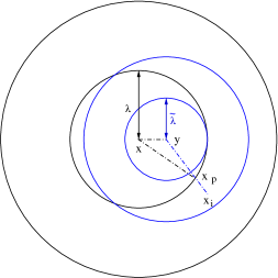
Figure 2: Geometric setting

$x_{i}$ is outside $B_{\lambda}(x)$ and $y$ is inside the ball. line segment between $y$ and $x_{i}$ is intersecting with the surface of the ball in one point. We call this point $x_{p}$ (See picture 2). We get

$$\left|x-x_{p}\right|\leq \left|x-y\right|+\left|y-x_{p}\right|\quad,$$

$$\left|y-x_{p}\right|\geq \left|x-x_{p}\right|-\left|x-y\right|=\lambda-\left|x-y\right|\geq\tilde{\lambda}\quad.$$ (55)

and

$$\left|x_{i}-y\right|= \left|x_{i}-x_{p}\right|+\left|x_{p}-y\right|\geq\left|x_{i}-x_{p}\right|+\tilde{\lambda}$$

$$\geq \frac{\tilde{\lambda}}{\lambda}\left|x_{i}-x_{p}\right|+\tilde{\lambda}\geq\frac{\left|x_{i}-x_{p}\right|+\lambda}{\lambda}\tilde{\lambda}\geq\frac{\left|x_{i}-x\right|}{\lambda}\tilde{\lambda}\quad.$$ (56)

Since $\varphi$ is monotone decreasing, we have

$$\varphi\left(\tilde{\lambda}^{-1}\left|x_{i}-y\right|\right)\leq\varphi\left(\tilde{\lambda}^{-1}\left|x_{i}-x\right|\right)\quad.$$ (57)

It holds

$$J_{\tilde{\lambda}}(\tilde{\mathcal{A}},\chi,y)= \frac{\left\|A^{-1}\right\|^{2}}{C_{\varphi}\tilde{\lambda}^{d}}\sum_{i}W(A\left(x_{i}-y\right)+\tau+A(y-x))\varphi\left(\tilde{\lambda}^{-1}\left|x_{i}-y\right|\right)$$

$$\leq \frac{\lambda^{d}}{\tilde{\lambda}^{d}}\frac{\left\|A^{-1}\right\|^{2}}{C_{\varphi}\lambda^{d}}\sum_{i}W(A\left(x_{i}-x\right)+\tau)\varphi\left(\lambda^{-1}\left|x_{i}-x\right|\right)$$

$$\leq\frac{\lambda^{d}}{\tilde{\lambda}^{d}}J_{\lambda}(\mathcal{A},\chi,x)\quad.$$ (58)

Now, we calculate a lower bound on $\rho_{\tilde{\lambda}}(\chi,y)$. We start at a Bravais lattice $\chi=\chi_{\mathcal{A}}+x=A^{-1}(\mathbb{Z}^{d}-\tau)+x$ as a configuration. This configuration has $\epsilon_{J}=0$ For this lattice we have $\rho_{\tilde{\lambda}}(\chi,y)=\det A+O(\lambda^{-2})$. There are different ways to reduce the density. On the one hand one can take atoms away. This decreases $\rho_{\tilde{\lambda}}(\chi,y)$ but because of equation (57) it also decreases $\rho_{\lambda}(\chi,x)$ at least by

$$\delta\rho_{\tilde{\lambda}}(\chi,y)<\frac{\lambda^{d}}{\tilde{\lambda}^{d}}\delta\rho_{\lambda}(\chi,x)\quad.$$ (59)

Another possibility is to move atoms to positions of lower $\varphi\left(\lambda^{-1}\left|x_{i}-x\right|\right)$ this does not have to reduce $\rho_{\lambda}(\chi,x)$ at all but it will increase $J_{\lambda}(\mathcal{A},\chi,x)$. If we shift the $i$‘th atom for a distance $\delta x_{i}$ we maximally reduce $\rho_{\tilde{\lambda}}(\chi,y)$ by

$$\delta\tilde{\rho}_{i}=\frac{1}{\lambda C_{\varphi}\tilde{\lambda}^{d}}\left|\nabla\varphi\right|\left(\lambda^{-1}\left|x_{i}-y\right|\right)\delta x_{i}+O(\lambda^{-1}\delta x_{i})\quad,$$ (60)

we get a minimal cost per atom of

$$\delta J_{i}<C_{0}^{W}\frac{1}{C_{\varphi}\tilde{\lambda}^{d}}\delta x_{i}^{2}\varphi\left(\lambda^{-1}\left|x_{i}-x\right|\right)+O(\lambda^{-1}\delta x_{i}^{2})\quad.$$ (61)

Furthermore, we have for $x_{i}\in B_{2\tilde{\lambda}}(y)$

$$\left|x_{i}-x\right|\leq \left|x_{i}-y\right|+\left|y-x\right|\leq 2\tilde{\lambda}+\lambda-\tilde{\lambda}<2\lambda\quad.$$ (62)

Therefore, it holds $\varphi\left(\lambda^{-1}\left|x_{i}-x\right|\right)>0$. If we minimize $\sum_{i}\delta J_{i}$ with the constrain $\rho_{\lambda}=\det A+\sum_{i}\delta\tilde{\rho}_{i}$, we get

$$J_{\lambda}>\left(\frac{\tilde{\lambda}}{\lambda}\right)^{d}\left(\frac{1}{C_{\varphi}\tilde{\lambda}^{d}}\sum_{x_{i}\in B_{2\tilde{\lambda}}(y)}\frac{\left|\nabla\tilde{\varphi}\right|^{2}\left(\lambda^{-1}\left(x_{i}-y\right)\right)}{\varphi\left(\lambda^{-1}\left|x_{i}-x\right|\right)}+O(\lambda^{-1})\right)^{-1}\lambda^{2}\delta\rho^{2}.$$ (63)

We estimate the sum over $\chi_{\mathcal{A}}$ by an integral using Lemma 9. The error is $O(\lambda^{-2})$ that means negligible compared to the error we already made.

$$J_{\lambda}\geq \left(\frac{\tilde{\lambda}}{\lambda}\right)^{d}\left(\frac{1}{C_{\varphi}\tilde{\lambda}^{d}}\int_{\mathbb{R}^{3}}\frac{\left|\nabla\varphi(\tilde{\lambda}^{-1}\left|z-y\right|)\right|^{2}}{\varphi\left(\lambda^{-1}\left|z-x\right|\right)}\det Adz+O(\lambda^{-1})\right)^{-1}\lambda^{2}\delta\rho^{2}\quad,$$

$$\delta\rho< \left(\frac{\lambda}{\tilde{\lambda}}\right)^{d/2}\left(\frac{1}{C_{\varphi}}\int_{\mathbb{R}^{3}}\frac{\left|\nabla\varphi(\left|z-y\right|)\right|^{2}}{\varphi\left(\left|z-x\right|\frac{\tilde{\lambda}}{\lambda}\right)}dz+O(\lambda^{-1})\right)^{\frac{1}{2}}\sqrt{\det A}\frac{\sqrt{J_{\lambda}}(A,\tau,\chi,x)}{\lambda}\quad,$$

$$\delta\rho< \tilde{C_{\rho}}\left(\frac{\lambda}{\tilde{\lambda}}\right)^{d/2}\frac{\sqrt{J_{\lambda}}(\mathcal{A},\chi,x)}{\lambda}\quad.$$ (64)

We can estimate the density $\rho_{\lambda}(\chi,x)$ from above with $\rho(\chi,x)<(1+\epsilon_{\rho})\det A$ We summarize the estimates (59) and (6) and we obtain

$$\det A-\rho_{\tilde{\lambda}}(\chi,y)<\left(\left(\frac{\lambda}{\tilde{\lambda}}\right)^{d/2}\frac{C+O(\lambda^{-1})}{\lambda}(1+\epsilon_{\rho})\epsilon_{J}+\left(\frac{\lambda}{\tilde{\lambda}}\right)^{d}\epsilon_{\rho}\right)\det A\quad.$$ (65)

If we start with a Bravais lattice and increase the density $\rho_{\tilde{\lambda}}(\chi,y)$ by changing the configuration there are two different ways. On the one hand can shift atoms to positions of higher $\varphi$. This leads to the same increase of $J_{\lambda}$ as in the reduction case. On the other hand one can add more atoms. This leads to the same increase of $\rho_{\lambda}(\chi,x)$ additionally it will increase $J_{\lambda}$ because new atoms can not be placed in the minima because all minima are occupied. We get the same estimate for the upper bound of $\rho_{\tilde{\lambda}}(\chi,y)$

$$\left|\det A-\rho_{\tilde{\lambda}}(\chi,y)\right|<\left(\left(\frac{\lambda}{\tilde{\lambda}}\right)^{d/2}\frac{C+O(\lambda^{-1})}{\lambda}(1+\epsilon_{\rho})\epsilon_{J}+\left(\frac{\lambda}{\tilde{\lambda}}\right)^{d}\epsilon_{\rho}\right)\det A\quad.$$ (66)

Finally, we estimate

$$J_{\tilde{\lambda}}(A,\tau,\chi,y)\leq \left(\frac{\lambda}{\tilde{\lambda}}\right)^{d}J_{\lambda}(A,\tau,\chi,x)\leq\left(\frac{\lambda}{\tilde{\lambda}}\right)^{d}\epsilon_{J}\rho_{\lambda}(\chi,x)\quad,$$

$$\leq \left(1+\tilde{\epsilon}_{\rho}\right)\left(\frac{\lambda}{\tilde{\lambda}}\right)^{d}\epsilon_{J}\det A\leq\left(\frac{\lambda}{\tilde{\lambda}}\right)^{d}\frac{1+\tilde{\epsilon}_{\rho}}{1-\epsilon_{\rho}}\epsilon_{J}\rho_{\tilde{\lambda}}(\chi,y)\quad.$$ (67)

Lemma 3

For all $C_{A}>s_{o}$ there exists $\hat{\lambda}\in\mathbb{R}$, $\epsilon_{\rho}>0$ and $\epsilon_{J}>0$ such that for all $\lambda>\hat{\lambda}$, $\mathcal{A}_{j}=(A_{j},\tau_{j})\in Gl_{d}(\mathbb{R})\times\mathbb{R}^{d}$ and $y_{j}\in B_{2\lambda}(\Omega)$ with $j=1,2,3$ the following holds. If $(y_{j},\mathcal{A}_{j})$ is $(\epsilon_{\rho},\epsilon_{J},C_{A})$-regular for $j=1,2,3$ and $|y_{j}-y_{k}|\leq\frac{3}{2}\lambda$ for $j,k=1,2,3$, then there exists uniquely defined reparametrisations $B_{j,k}\in Gl_{d}(\mathbb{Z})$, $t_{j,k}\in Z^{d}$ճuch that

$$\|id-A_{j}^{-1}B_{j,k}A_{k}\|< \frac{c^{A}_{J}}{\sqrt{\det A_{k}}}\left(\frac{2\lambda}{2\lambda-|y_{j}-y_{k}|}\right)^{d/2}\frac{\sqrt{J_{j,k}}}{\lambda},$$

$$\left|\delta\tau_{j,k}\right|< \frac{c^{\tau}_{J}|A_{j}|}{\sqrt{\det A_{k}}}\left(\frac{2\lambda}{2\lambda-\left|y_{j}-y_{k}\right|}\right)^{d/2}\sqrt{J_{j,k}},$$ (68)

where

$$\delta\tau_{j,k}:= B_{j,k}՜tau_{k}+t_{j,k}-\tau_{j}-\frac{B_{j,k}A_{k}+A_{j}}{2}\left(y_{k}-y_{j}\right)\quad,$$

$$J_{j,k}:= \max\left\{J_{\lambda}(\mathcal{A}_{j},\chi,y_{j}),J_{\lambda}(\mathcal{A}_{k},\chi,y_{k})\right\}\quad,$$

$$c^{A}_{J}:= \frac{3}{2}\left(\frac{8dC_{\varphi}}{C_{\varphi 2}C_{0}^{W}}\right)^{\frac{1}{2}}\quad,\quad c^{\tau}_{J}:=\left(\frac{10}{C_{0}^{W}}\right)^{\frac{1}{2}}\quad.$$ (69)

Moreover, it holds

$$B_{1,3}= B_{1,2}B_{2,3}\quad,$$

$$t_{1,3}= B_{1,2}t_{2,3}+t_{1,2}$$ (70)

Proof

We consider $\bar{y}=(y_{j}+y_{k})/2$ and get

$$\left|y_{j}-\bar{y}\right|=\left|y_{k}-\bar{y}\right|=\left|y_{j}-y_{k}\right|/2<3/4\lambda$$ (71)

We apply Lemma 2 twice, one time with $y_{j}$ as $x$ and $\bar{y}$ as $y$ and the other time with $y_{k}$ as $x$ and $\bar{y}$ as $y$. $(\bar{y},\tilde{\mathcal{A}}_{j}:=(A_{j},\tau_{j}+A_{j}\left(x_{k}-x_{j}\right)/2)$ and $(\bar{y},\tilde{\mathcal{A}}_{k}:=(A_{k},\tau_{k}+A_{k}\left(x_{j}-x_{k}\right)/2))$ are $\left(\tilde{\epsilon}_{J},\tilde{\epsilon}_{\rho},C_{A}\right)$-regular. Therefore, we get

$$J_{\lambda}(\tilde{\mathcal{A}}_{j},\chi,\bar{y})= \left(\frac{2\lambda}{2\lambda-\left|y_{j}-y_{k}\right|}\right)^{d}J_{\tilde{\lambda}}(x,A,\tau+A(\bar{y}-x_{j}))\quad,$$

$$\tilde{\epsilon}_{\rho}= \left(\frac{2\lambda}{2\lambda-\left|y_{j}-y_{k}\right|}\right)^{d/2}\frac{C+O(\lambda^{-1})}{\lambda}(1+\epsilon_{\rho})\epsilon_{J}+\left(\frac{2\lambda}{2\lambda-\left|y_{j}-y_{k}\right|}\right)^{d}\epsilon_{\rho}.$$ (72)

Since we have two regular pairs, we can apply Lemma 1 and get $B_{j,k}\in\rm{GL}_{d}(\mathbb{Z})$ and $t_{j,k}\in\mathbb{Z}^{d}$ such that

$$\|1-A_{j}^{-1}B_{j,k}A_{k}\|< \frac{C^{A}_{J}}{\sqrt{\det A_{k}}}\left(\frac{2\lambda}{2\lambda-|y_{j}-y_{k}|}\right)^{d/2}\frac{\sqrt{J_{\lambda}}}{\lambda}\quad,$$

$$\left|B_{j,k}\tau_{k}-\tau_{j}+\frac{B_{j,k}A_{k}+A_{j}}{2}\left(y_{k}-y_{j}\right)+t\right|< \frac{c^{\tau}_{J}\|A_{j}|}{\sqrt{\det A_{k}}}\left(\frac{2\lambda}{2\lambda-\left|y_{j}-y_{k}\right|}\right)^{d/2}\sqrt{J_{j,k}}.$$ (73)

This proves the first part of the theorem. Since it holds $|A_{j}^{-1}|\leq C_{A}$, the matrix derivative of $\det A_{j}$ is bounded. Additionally, it holds $\det A_{j}<(1-\epsilon_{\rho})^{-1}\rho^{max}_{d}$. Hence, the estimate (6) implies that we can estimate

$$\det A_{j}=\det A_{k}+O\left(\frac{\sqrt{J_{\lambda}}}{\lambda}\right)\quad.$$ (74)

Due to the regularity condition on the density we get $\rho_{\lambda}(\chi,x_{j})<(1+\epsilon_{\rho})\det A_{j}$. Therefore, we get for small enough $\epsilon_{J}$

$$J_{j,k} =\max\left\{J_{\lambda}(\mathcal{A}_{j},\chi,y_{j}),J_{\lambda}(\mathcal{A}_{k},\chi,y_{k})\right\}\leq\epsilon_{J}\max\left\{\rho_{\lambda}(\chi,y_{j}),\rho_{\lambda}(\chi,y_{k})\right\}\quad$$

$$\leq \epsilon_{J}(1+\epsilon_{\rho})\max\left\{\det A,\det A_{k}\right\}\leq\quad\epsilon_{J}(1+\epsilon_{\rho})\left(1+O\left(\frac{\sqrt{J_{\lambda}}}{\lambda}\right)\right)\det A_{k}\quad.$$ (75)

Hence, for sufficiently large $\lambda$ we have

$$\|id-A_{j}^{-1}B_{j,k}A_{k}\|< 2c^{A}_{J}2^{d+1}\frac{\sqrt{\epsilon_{J}}}{\lambda}\quad.$$ (76)

We calculate for $\epsilon_{J}$ small enough

$$\left|id-A^{-1}_{1}B_{1,2}B_{2,3}A_{3}\right|\leq \left|id-A^{-1}_{1}B_{1,2}A_{2}+A^{-1}_{1}B_{1,2}A_{2}\left(1-A_{2}^{-1}B_{2,3}A_{3}\right)\right|$$

$$\leq \left|id-A_{1}^{-1}B_{1,2}A_{2}\right|+\left|A^{-1}_{1}B_{1,2}A_{2}\right|\left|id-A_{1}^{-1}B_{2,3}A_{3}\right|$$

$$\leq 6c^{A}_{J}2^{d}\frac{\sqrt{\epsilon_{J}}}{\lambda}\quad.$$ (77)

Due to the estimate (76) we know

$$\|id-A_{1}^{-1}B_{1,3}A_{3}\|<2c^{A}_{J}2^{d}\frac{\sqrt{\epsilon_{J}}}{\lambda}\quad.$$ (78)

We get for $\epsilon_{J}<\lambda^{2}(8C_{A}C_{|A|}C^{A}_{J}2^{d})^{-2}$

$$\left|B_{1,3}-B_{1,2}B_{2,3}\right|\leq \left|A_{1}\right|\left|A_{1}^{-1}\left(B_{1,3}-B_{1,2}B_{2,3}\right)A_{3}\right|\left|A^{-1}_{3}\right|$$

$$\leq C_{A}C_{|A|}\left|A_{1}^{-1}B_{1,3}A_{3}-A_{1}^{-1}B_{1,2}B_{2,3}A_{3}\right|$$

$$\leq C_{A}C_{|A|}\left(\left|id-A_{1}^{-1}B_{1,3}A_{3}\right|+\left|id-A_{1}^{-1}B_{1,2}B_{2,3}A_{3}\right|\right)$$

$$\leq 8c^{A}_{J}C_{A}C_{|A|}2^{d}\frac{\sqrt{\epsilon_{J}}}{\lambda}<1\quad.$$ (79)

The distance between $B_{1,3}$ and $B_{1,2}B_{2,3}$ is smaller than one and they are both elements of the discrete set $Gl_{d}(\mathbb{Z})$. Therefore, they have to be equal. $B_{1,3}=B_{1,2}B_{2,3}$ also implies the uniqueness of $B_{1,3}$ and because $B_{1,2}$ and $B_{2,3}$ are invertible also the uniqueness of $B_{1,2}$ and $B_{2,3}$. Next, we need prove $t_{1,2}+B_{1,2}t_{2,3}=t_{1,3}$. If we apply estimate (6) on (6) for the first chain, we get

$$\delta\tau_{j,k}:= B_{j,k}\tau_{k}+t_{j,k}-\tau_{j}-\frac{B_{j,k}A_{k}+A_{j}}{2}\left(y_{k}-y_{j}\right)\quad,$$

$$\left|\delta\tau_{j,k}\right|< 2c^{\tau}_{J}C_{|A|}2^{d}\sqrt{\epsilon_{J}}\quad.$$ (80)

Due to the estimates (6) and (6) it holds for $\epsilon_{J}<\lambda^{2}(c^{A}_{J}2^{d})^{-2}$

$$\left|B_{1,2}A_{2}-A_{1}\right|\leq \left|A_{1}^{-1}B_{1,2}A_{2}-id\right|\left|A_{2}\right|\leq 2C_{|A|}c^{A}_{J}2^{d}\frac{\sqrt{\epsilon_{J}}}{\lambda}\quad,$$

$$\left|B_{1,2}A_{2}-B_{1,2}B_{2,3}A_{3}\right|\leq \left|B_{1,2}A_{2}\right|\left|id-A_{2}^{-1}B_{2,3}A_{3}\right|\leq 2\left|A_{1}\right|\left|A_{1}^{-1}B_{1,2}A_{2}\right|c^{A}_{J}2^{d}\frac{\sqrt{\epsilon_{J}}}{\lambda}$$

$$\leq 2C_{|A|}\left(1+2c^{A}_{J}2^{d}\frac{\sqrt{\epsilon_{J}}}{\lambda}\right)c^{A}_{J}2^{d}\frac{\sqrt{\epsilon_{J}}}{\lambda}\leq 4C_{|A|}c^{A}_{J}2^{d}\frac{\sqrt{\epsilon_{J}}}{\lambda}\quad.$$ (81)

We also get

$$\left|B_{1,2}\right|\leq\left|A_{1}\right|\left|A_{1}^{-1}B_{1,2}A_{2}\right|\left|A_{2}^{-1}\right|\leq C_{A}C_{|A|}\left(1+2c^{A}_{J}2^{d}\frac{\sqrt{\epsilon_{J}}}{\lambda}\right)\leq 2C_{A}C_{|A|}\quad.$$ (82)

Hence, we can estimate

$$\left|B_{1,2}B_{2,3}\tau_{3}+B_{1,2}t_{2,3}+t_{1,2}-\tau_{1}-\frac{B_{1,2}B_{2,3}A_{3}+A_{1}}{2}\left(y_{3}-y_{1}\right)\right|$$

$$= \left|\frac{B_{1,2}A_{2}+A_{1}}{2}\left(y_{2}-y_{1}\right)+B_{1,2}\frac{B_{2,3}A_{3}+A_{2}}{2}\left(y_{3}-y_{2}\right)-\frac{B_{1,2}B_{2,3}A_{3}+A_{1}}{2}\left(y_{3}-y_{1}\right)\right|$$

$$+\left|B_{1,2}\delta\tau_{2,3}+\delta\tau_{1,2}\right|$$

$$\leq \left|B_{1,2}\delta\tau_{2,3}\right|+\left|\delta\tau_{1,2}\right|+\frac{1}{2}\left|\left(B_{1,2}A_{2}-A_{1}\right)\left(y_{3}-y_{2}\right)\right|+\frac{1}{2}\left|\left(B_{1,2}A_{2}-B_{1,2}B_{2,3}A_{2}\right)\left(y_{2}-y_{1}\right)\right|$$

$$\leq \left|B_{1,2}\right|\left|\delta\tau_{2,3}\right|+\left|\delta\tau_{1,2}\right|+\frac{3\lambda}{4}\left|B_{1,2}A_{2}-A_{1}\right|+\frac{3\lambda}{4}\left|B_{1,2}A_{2}-B_{1,2}B_{2,3}A_{3}\right|\quad.$$ (83)

We use the estimates (6), (6) and (82).

$$\left|B_{1,2}B_{2,3}\tau_{3}+B_{1,2}t_{2,3}+t_{1,2}-\tau_{1}-\frac{B_{1,2}B_{2,3}A_{3}+A_{1}}{2}\left(y_{3}-y_{1}\right)\right|$$

$$\leq \left(\left(4C_{A}C_{|A|}+2\right)c^{\tau}_{J}+9/2C^{A}_{J}\right)2^{d}C_{|A|}\sqrt{\epsilon_{J}}\quad.$$ (84)

On the other hand, if we apply the estimate to the second chain, we get

$$\left|B_{1,2}B_{2,3}\tau_{3}+t_{1,3}-\tau_{1}-\frac{B_{1,2}B_{2,3}A_{3}+A_{1}}{2}\left(y_{3}-y_{1}\right)\right|< 2c^{\tau}_{J}C_{|A|}2^{d}\sqrt{\epsilon_{J}}\quad.$$ (85)

Hence, if we denote $X:=B_{1,2}B_{2,3}\tau_{3}-\tau_{1}-\frac{B_{1,2}B_{2,3}A_{3}+A_{1}}{2}\left(y_{3}-y_{1}\right)$, we finally get with the estimates (6) and (85)

$$\left|B_{1,2}t_{2,3}+t_{1,2}-t_{1,3}\right|\leq \left|B_{1,2}t_{2,3}+t_{1,2}+X\right|+\left|X-t_{1,3}\right|$$

$$\leq \left((4C_{A}C_{|A|}+2)c^{\tau}_{J}+9/2c^{A}_{J}\right)2^{d}C_{|A|}\sqrt{\epsilon_{J}}\quad.$$ (86)

For $\epsilon_{J}<\left(\left((4C_{A}c_{|A|}+2)c^{\tau}_{J}+9/2c^{A}_{J}\right)2^{d}C_{|A|}\right)^{-2}$ the difference between $B_{1,2}t_{2,3}+t_{1,2}$ and $t_{2,3}$ is smaller than $1$ and since both belong to the discrete set $\mathbb{Z}^{d}$, they have to be equal. As in the case of $B$ the equation $B_{1,2}t_{2,3}+t_{1,2}=t_{1,3}$ implies the uniqueness of $t_{j,k}$.

Proof of Theorem 4.1

Proof

For sufficiently large $\lambda$ and small $\epsilon_{J}$ the conditions Lemma 3 are fulfilled for any $j$, if we take $y_{j}$ as the first point in Lemma 3 $y_{j+1}$ as the second and the third point. Hence, we get a sequence $\mathcal{B}_{j,j+1}$ fulfilling equation 1 for every $j$. Furthermore, we can apply Lemma 3 on the three points $y_{k-1}$, $y_{k+1}$ and $y_{k}$ From the first part of Lemma 3 we get the existence of a reparametrisation $\mathcal{B}_{k-1,k+1}$ between $y_{k-1}$ and $y_{k+1}$. Due to equation (3) Lemma 3 we get:

$$B_{k-1,k}B_{k,k+1}= B_{k-1,k+1}\quad,$$

$$t_{k-1,k}+B_{k-1,k}t_{k,k+1}= t_{k-1,k+1}\quad.$$ (87)

Therefore, we get equation (20).

7 Proof of Theorem 4.2

The next lemma shows that low energy points are regular.

Lemma 4

If $H(\chi)<\infty$ and $\hat{h}_{\lambda}(\chi,x)\leq\epsilon\leq\frac{1}{4}\min\left\{C_{1}^{El}\det(E)^{2},C_{2}^{El}|E|^{2},\vartheta\det E\right\}$, then there exists $\hat{\mathcal{A}}\in Gl_{d}(\mathbb{R}^{d})\times\mathbb{R}^{d}$ such that $\hat{h}_{\lambda}(\chi,x)=h_{\lambda}(\hat{\mathcal{A},\chi,x})$ and $(x,\hat{\mathcal{A}}9$ is $(\epsilon_{\rho},\epsilon_{J},C_{A})$-regular; where

$$C_{A}=\frac{3^{d-1}|E|^{d-1}}{2^{d-2}\det E}\quad,\quad\epsilon_{\rho}=2\vartheta\frac{\epsilon}{\det E}\quad,\quad\epsilon_{J}=\frac{4\epsilon}{\det E}\quad.$$ (88)

Additionally $\det\hat{A}\leq\frac{3}{2}\det E$

Proof

For a configuration of finite energy the hard core condition $|x_{i}-x_{j}|>s_{o}$ is fulfilled for all atoms. Furthermore, for all $\mathcal{A}\in Gl(\mathbb{R})\times\mathbb{R}^{d}$ satisfying

$$\epsilon\geq h_{\lambda}\left(\mathcal{A},\chi x\right)=F\left(A\right)+J_{\lambda}\left(\mathcal{A},\chi,x\right)+\nu_{\lambda}\left(\chi,A,x\right)$$ (89)

it holds due to the positivity of $F$, $J_{\lambda}$ and $\nu_{\lambda}$

$$F\left(A\right)\leq\epsilon\quad,\quad J_{\lambda}\left(\mathcal{A},\chi,x\right)\leq\epsilon\quad,\quad\nu_{\lambda}\left(\chi,A,x\right)\leq\epsilon\quad,$$ (90)

Hence, we have

$$\epsilon\geq F(A)\geq C_{1}^{El}\left(\det(E)-\det(A))\right)^{2}+C_{2}^{El}\text{dist}^{2}\left(A,E\;SO_{d}\right)\quad.$$ (91)

Therefore, for $\epsilon\leq\frac{1}{4}\min\left\{C_{1}^{El}\det(E)^{2},C_{2}^{El}|E|^{2}\right\}$ we have

$$\frac{1}{2}\det E \leq\det(A)\leq\frac{3}{2}\det E\quad,$$

$$\frac{1}{2}|E| \leq|A|\leq\frac{3}{2}|E|\quad.$$ (92)

Additionally we have

$$|A^{-1}|\leq |A|^{d-1}\det A^{-1}\leq\frac{3^{d-1}|E|^{d-1}}{2^{d-2}\det E}\quad,$$

$$|A^{-1}|\geq \left(|A|\det A^{-1}\right)^{\frac{1}{d-1}}\geq\left(\frac{|E|}{3\det E}\right)^{\frac{1}{d-1}}\quad.$$ (93)

Because $h_{\lambda}\left(\cdot,\chi,x\right)$ is periodic in $\tau$, we can restrict $\tau$ to the compact set $[0,1]^{d}$. Hence, $Gl_{d}^{\epsilon}:=\left\{\mathcal{A}\in Gl_{d}(\mathbb{R})|h_{\lambda}(\mathcal{A},\chi,x)\leq\epsilon,\tau\in[0,1]^{d}\right\}$ is a compact subset of $Gl_{d}(\mathbb{R})\times\mathbb{R}^{d}$. Since it holds $\hat{h}_{\lambda}(\chi,x)=\inf_{\mathcal{A}}\left\{h_{\lambda}\left(\mathcal{A},\chi,x\right)\right\}<\epsilon$, the set $Gl_{d}^{\epsilon}\times[0,1]^{d}$ is not empty. Hence, the continuous function $h_{\lambda}\left(\cdot,\chi,x\right)$ attains a minimum $\hat{\mathcal{A}}=(\hat{A},\hat{\tau})$ on the compact set $Gl_{d}^{\epsilon}\times[0,1]^{d}$ that is per definition the global minimizer of $h_{\lambda}\left(\cdot,\chi,x\right)$. Due to the estimates (90) $\hat{\mathcal{A}}$ satisfies

$$\vartheta\left|\det A-\rho_{\lambda}(\chi,x)\right|\leq\nu_{\lambda}\left(A,\chi,x\right)\leq 2\frac{\epsilon}{\det E}\det A\quad.$$ (94)

If we use the estimates (94) and (90), we obtain for $\epsilon\leq\frac{1}{4}\vartheta\det E$

$$J_{\lambda}(\mathcal{A},\chi,x)<\epsilon<\frac{\epsilon}{2^{-1}\det A-\vartheta^{-1}\epsilon}\rho_{\lambda}(\chi,x)\leq\frac{4\epsilon}{\det E}\rho_{\lambda}(\chi,x)$$ (95)

$J_{\lambda}$ is locally convex in $\mathcal{A}$ for regular pairs.

Lemma 5

For all $C_{A}$ there exists $\hat{\lambda},\epsilon_{J}$ such that for all $\lambda>\hat{\lambda}$, for all $(C_{A},\epsilon_{\rho},\epsilon_{J})$-regular $(x,\mathcal{A})=(x,(A,\tau))\in\in B_{2\lambda}(\Omega)\times Gl_{d}(\mathbb{R})\times\mathbb{R}^{d}$ and all test matrices $\mathcal{M}=(M,\mu)\in\mathbb{R}^{d\times d}\times\mathbb{R}^{d}$ it holds

$$\partial_{\mathcal{A}}^{2}J_{\lambda}(\mathcal{A},\chi,x)[\mathcal{M}]\geq C_{Con}\left\|A^{-1}\right\|^{2}\rho_{\lambda}\|\mathcal{M}\|_{\lambda}^{2}\quad,$$ (96)

where $C_{con}$ is defined by

$$C_{con}:=c_{\Theta}^{0}\min\left\{\frac{1}{12},\frac{c_{\Theta}^{0}C_{\varphi}^{2}}{4\left(9+d\right)w_{d-1}^{2}4^{d}}\frac{\rho_{\lambda}^{2}}{\det A^{2}}\right\}\quad.$$ (97)

Proof

The second derivative $\partial_{\mathcal{A}}^{2}J_{\lambda}$ tested by $\mathcal{M}=(M,\mu)\in\mathbb{R}^{d\times d}\times\mathbb{R}^{d}$ is given by

$$\partial_{\mathcal{A}}^{2}J_{\lambda}(\mathcal{A},\chi,x)[\mathcal{M}]= \frac{\left\|A^{-1}\right\|^{2}}{C_{\varphi}\lambda^{d}}\sum_{i}\nabla^{2}W(A\left(x_{i}-x\right)+\tau)[M(x_{i}-x)+\mu]\varphi$$

$$+2\frac{\partial_{\mathcal{A}}\left\|A^{-1}\right\|^{2}[M]}{C_{\varphi}\lambda^{d}}\sum_{i}\left<\nabla W(A\left(x_{i}-x\right)+\tau),M(x_{i}-x)+\mu\right>\varphi$$

$$+\frac{\partial_{\mathcal{A}}^{2}\left\|A^{-1}\right\|^{2}[M]}{C_{\varphi}\lambda^{d}}\sum_{i}W(A\left(x_{i}-x\right)+\tau)\varphi\quad.$$ (98)

The two last terms lower are of order $O(\lambda^{-1})\|\mathcal{M}\|_{\lambda}$. Furthermore, we can split the first sum into one sum over the regular atoms $\chi_{\mathcal{A},\beta,x}^{reg}$ with $\beta=\min\left\{|A|^{-1}\Theta_{W},s_{o}/3\right\}$ and one sum over the irregular atoms, and get

$$C_{\varphi}\lambda^{d}\partial_{\mathcal{A}}^{2}J_{\lambda}(\mathcal{A},\chi,x)[\mathcal{M}]= \left\|A^{-1}\right\|^{2}\sum_{x_{i}\in\chi_{\mathcal{A},\beta,x}^{reg}}\nabla^{2}W(A\left(x_{i}-x\right)+\tau)[M(x_{i}-x)+\mu]\varphi$$

$$+\left\|A^{-1}\right\|^{2}\sum_{x_{i}\in\chi_{\mathcal{A},\beta,x}^{irr}}\nabla^{2}W(A\left(x_{i}-x\right)+\tau)[M(x_{i}-x)+\mu]\varphi$$

$$-O(\lambda^{-1})\|\mathcal{M}\|_{\lambda}^{2}.$$ (99)

On the one hand all the regular atoms satisfy

$$dist(x_{i},\chi_{\mathcal{A}}+x)\leq \beta\quad,$$

$$dist(A(x_{i}-x)+\tau,\mathbb{Z}^{d})\leq \beta|A|\leq\Theta_{W}\quad,$$

$$c_{\Theta}^{0}(M(x_{i}-x)+\mu)^{2}\leq \nabla^{2}W(A\left(x_{i}-x\right)+\tau)[M(x_{i}-x)+\mu]\quad.$$ (100)

Since $W$ is two times differentiable and periodic, there is an upper bound for its second derivative, which we can use to bound the contribution of the irregular atoms. Hence, we get

$$\partial_{\mathcal{A}}^{2}J_{\lambda}(\mathcal{A},\chi,x)[\mathcal{M}]\geq c_{\Theta}^{0}\frac{\left\|A^{-1}\right\|^{2}}{C_{\varphi}\lambda^{d}}\sum_{x_{i}\in\chi_{\mathcal{A},\beta,x}^{reg}}(M(x_{i}-x)+\mu)^{2}\varphi\left(\lambda^{-1}\left|x_{i}-x\right|\right)$$

$$-8\left\|A^{-1}\right\|^{2}\|\nabla^{2}W\|_{\infty}\rho_{\mathcal{A},\beta}^{irr}(x)\|\mathcal{M}\|_{\lambda}^{2}-O(\lambda^{-1})\|\mathcal{M}\|_{\lambda}^{2}\quad.$$ (101)

We define the average particle position by

$$\bar{x}:=\left(\rho_{\mathcal{A},\beta}^{reg}(x)\right)^{-1}\frac{1}{C_{\varphi}\lambda^{d}}\sum_{x_{i}\in\chi_{\mathcal{A},\beta,x}^{reg}}x_{i}\varphi\left(\lambda^{-1}\left|x_{i}-x\right|\right)\quad.$$ (102)

Using this definition we get

$$\partial_{\mathcal{A}}^{2}J_{\lambda}(\mathcal{A},\chi,x)[\mathcal{M}]\geq c_{\Theta}^{0}\frac{\left\|A^{-1}\right\|^{2}}{C_{\varphi}\lambda^{d}}\sum_{x_{i}\in\chi_{\mathcal{A},\beta,x}^{reg}}\left(\left(M(x_{i}-\bar{x})\right)^{2}+\left(M(\bar{x}-x)+\mu\right)^{2}\right)\varphi$$

$$-\left\|A^{-1}\right\|^{2}\|\nabla^{2}W\|_{\infty}\rho_{\mathcal{A},\beta}^{irr}(x)+O(\lambda^{-1})\|\mathcal{M}\|_{\lambda}^{2}\quad.$$ (103)

Because $(M(\bar{x}-x)+\mu)^{2}$ is independent of $i$, this sum can be expressed with the density of regular atoms. If we denote by $e_{M}$ the eigenvector the largest eigenvalue of $M^{T}M$, we get

$$\partial_{\mathcal{A}}^{2}J_{\lambda}(\mathcal{A},\chi,x)[\mathcal{M}]\geq c_{\Theta}^{0}\frac{\left\|A^{-1}\right\|^{2}}{C_{\varphi}\lambda^{d}}\sum_{x_{i}\in\chi_{\mathcal{A},\beta,x}^{reg}}\left(e_{m}(x_{i}-\bar{x})\right)^{2}|M|^{2}\varphi$$

$$+c_{\Theta}^{0}\left\|A^{-1}\right\|^{2}(M(\bar{x}-x)+\mu)^{2}\rho_{\mathcal{A},\beta}^{reg}(x)$$

$$-8\left\|A^{-1}\right\|^{2}\|\nabla^{2}W\|_{\infty}\rho_{\mathcal{A},\beta}^{irr}(x)\|\mathcal{M}\|_{\lambda}^{2}+O(\lambda^{-1})\|\mathcal{M}\|_{\lambda}^{2}\quad.$$ (104)

We concentrate on the calculation of

$$X:=\frac{1}{C_{\varphi}\lambda^{d}}\sum_{x_{i}\in\chi_{\mathcal{A},\beta,x}^{reg}}\left(e_{m}(x_{i}-\bar{x})\right)^{2}\varphi\left(\lambda^{-1}\left|x_{i}-x\right|\right)\quad.$$ (105)

Due to $\beta\leq s_{o}/3$ there can be only one regular atom in $B_{\beta}(A^{-1}(z_{i}-\tau)+x)$ for any $z_{i}$ Therefore, the regular atoms can not sit all on the plain $P:=\{y\in R^{d}|e_{m}(y-\bar{x})=0\}$. We call $h$ the minimal distance to the plain $P$ up to which we have to fill atoms to reach the density $\rho_{\mathcal{A},\beta}^{reg}(x)$. We define the cylinder

$$Z_{P}:=\left\{y\left|\left|\left<e_{M},y-x\right>\right|\leq 2\lambda\right.\right\}\quad.$$ (106)

The characteristic function $1_{Z_{P}}$ of this set satisfies:

$$1_{Z_{P}}(x)\geq\varphi\left(\lambda^{-1}\left|x_{i}-x\right|\right)\quad.$$ (107)

Hence, it holds

$$C_{\varphi}\lambda^{d}\rho_{\mathcal{A},\beta}^{reg}(x)= \sum_{x_{i}\in\chi_{\mathcal{A},\beta,x}^{reg}}\varphi\left(\lambda^{-1}\left|x_{i}-x\right|\right)\leq\sum_{x_{i}\in\chi_{\mathcal{A},\beta,x}^{reg}}1_{Z_{P}}(x_{i})\leq 2w_{d-1}(2\lambda)^{d-1}\det Ah\quad.$$ (108)

and we get

$$h\geq\frac{C_{\varphi}\lambda\rho_{\mathcal{A},\beta}^{reg}(x)}{w_{d-1}2^{d}\det A}\quad.$$ (109)

Since for any valley with distance less then $h$ from the plain $P$, that does not have a regular atom, there needs to be an regular atom with larger distance to reach the same density. Filling the whole cylinder gives us a lower bound for $X$

$$X\geq \frac{1}{C_{\varphi}\lambda^{d}}\int_{0}^{h}2\tilde{h}^{2}w_{d-1}(2\lambda)^{d-1}\det Ad\tilde{h}\geq\frac{C_{\varphi}^{2}}{3w_{d-1}^{2}4^{d}}\lambda^{2}\det A^{-2}\left(\rho_{\mathcal{A},\beta}^{reg}\right)^{3}\quad.$$ (110)

We apply this on the estimate (7) and get

$$\partial_{\mathcal{A}}^{2}J_{\lambda}(\mathcal{A},\chi,x)[\mathcal{M}]\geq c_{\Theta}^{0}\left\|A^{-1}\right\|^{2}|M|^{2}\frac{C_{\varphi}^{2}}{3w_{d-1}^{2}4^{d}}\lambda^{2}\det A^{-2}\left(\rho_{\mathcal{A},\beta}^{reg}\right)^{3}$$

$$+c_{\Theta}^{0}\left\|A^{-1}\right\|^{2}(M(\bar{x}-x)+\mu)^{2}\rho_{\mathcal{A},\beta}^{reg}(x)$$

$$-\left\|A^{-1}\right\|^{2}\|\nabla^{2}W\|_{\infty}\rho_{\mathcal{A},\beta}^{irr}(x)+O(\lambda^{-1})\|\mathcal{M}\|_{\lambda}^{2}\quad.$$ (111)

We treat two cases. In case one it holds $|\mu|<3\lambda|M|$. In case two holds $|\mu|\geq 3\lambda|M|$. For case one we calculate

$$(9+d)\lambda^{2}|M|^{2}\geq d\lambda^{2}|M|^{2}+|\mu|^{2}=\lambda^{2}\|M\|^{2}+|\mu|^{2}=\|\mathcal{M}\|_{\lambda}^{2}\quad.$$ (112)

We apply this to the estimate (7) and get

$$\partial_{\mathcal{A}}^{2}J_{\lambda}(\mathcal{A},\chi,x)[\mathcal{M}]\geq \frac{c_{\Theta}^{0}C_{\varphi}^{2}}{3\left(9+d\right)w_{d-1}^{2}4^{d}}\left\|A^{-1}\right\|^{2}\det A^{-2}\left(\rho_{\mathcal{A},\beta}^{reg}\right)^{3}\|\mathcal{M}\|_{\lambda}^{2}$$

$$-8\left\|A^{-1}\right\|^{2}\|\nabla^{2}W\|_{\infty}\rho_{\mathcal{A},\beta}^{irr}(x)+O(\lambda^{-1})\|\mathcal{M}\|_{\lambda}^{2}\quad.$$ (113)

Since every atom contributing to the average $\bar{x}$ is in $B_{2\lambda}(x)$, also $\bar{x}$ itself has to be in $B_{2\lambda}(x)$. Therefore, we obtain for case two

$$(M(\bar{x}-x)+\mu)^{2}\geq\left(|\mu|-|M||\bar{x}-x|\right)^{2}\geq\left(|\mu|-|M|2\lambda\right)^{2}\geq\frac{1}{9}|\mu|^{2}\quad.$$ (114)

With estimate (7) we get

$$\partial_{\mathcal{A}}^{2}J_{\lambda}(\mathcal{A},\chi,x)[\mathcal{M}]\geq c_{\Theta}^{0}\left\|A^{-1}\right\|^{2}\|M\|^{2}\frac{dC_{\varphi}^{2}}{3dw_{d-1}^{2}4^{d}}\lambda^{2}\det A^{-2}\left(\rho_{\mathcal{A},\beta}^{reg}\right)^{3}+\frac{c_{\Theta}^{0}}{9}\left\|A^{-1}\right\|^{2}|\mu|^{2}\rho_{\mathcal{A},\beta}^{reg}(x)$$

$$-\left\|A^{-1}\right\|^{2}\|\nabla^{2}W\|_{\infty}\rho_{\mathcal{A},\beta}^{irr}(x)+O(\lambda^{-1})\|\mathcal{M}\|_{\lambda}^{2}\quad.$$ (115)

We summarize the inequalities (7) and (7) to get

$$\partial_{\mathcal{A}}^{2}J_{\lambda}(\mathcal{A},\chi,x)[\mathcal{M}]\leq c_{\Theta}^{0}\left\|A^{-1}\right\|^{2}\rho_{\mathcal{A},\beta}^{reg}(x)\alpha\|\mathcal{M}\|_{\lambda}^{2}-\left\|A^{-1}\right\|^{2}\|\nabla^{2}W\|_{\infty}\rho_{\mathcal{A},\beta}^{irr}(x)+O(\lambda^{-1})\|\mathcal{M}\|_{\lambda}^{2}\quad.$$ (116)

where $\alpha$ is defined by

$$\alpha:=\min\left\{\frac{1}{9},\frac{c_{\Theta}^{0}C_{\varphi}^{2}}{3\left(9+d\right)w_{d-1}^{2}4^{d}}\frac{\left(\rho_{\mathcal{A},\beta}^{reg}\right)^{2}}{(\det A)^{2}}\right\}\quad.$$ (117)

We know from Lemma 11 with $\beta:=\min\{|A|^{-1}\Theta_{W},s_{o}/3\}$ that it holds

$$\rho_{\mathcal{A},\beta}^{irr}(x)\leq \frac{1}{C_{0}^{W}\min\{|A|^{-1}\Theta_{W},s_{o}/3\}^{2}}J_{\lambda}(\mathcal{A},\chi,x)\quad,$$ (118)

$$\rho_{\mathcal{A},\beta}^{reg}(x)\geq \rho_{\lambda}(\chi,x)-\frac{1}{C_{0}^{W}\min\{|A|^{-1}\Theta_{W},s_{o}/3\}^{2}}J_{\lambda}(\mathcal{A},\chi,x)\quad.$$ (119)

Therefore, we can control $\rho_{\mathcal{A},\beta}^{irr}$ and $\rho_{\lambda}-\rho_{\mathcal{A},\beta}^{reg}(x)$ for sufficiently low $\epsilon_{J}$ and large $\lambda$ arriving at

$$\partial_{\mathcal{A}}^{2}J_{\lambda}(\mathcal{A},\chi,x)[\mathcal{M}]\geq\frac{7}{8}\alpha c_{\Theta}^{0}\left\|A^{-1}\right\|^{2}\rho_{\lambda}(x)\|\mathcal{M}\|_{\lambda}^{2}\quad.$$ (120)

Lemma 6

For all configurations $\chi$ and all $\mathcal{A}\in Gl_{d}(\mathbb{R})\times\mathbb{R}^{d}$ we have

$$J_{\lambda}(\mathcal{A},\chi,x)\geq\alpha_{\nabla}^{-1}\left\|A^{-1}\right\|^{2}C_{\varphi}^{-1}\lambda^{-d}\sum_{i}|\nabla W|^{2}(A\left(x_{i}-x\right)+\tau)\varphi\left(\lambda^{-1}|x-x_{i}|\right)\quad,$$ (121)

where

$$\alpha_{\nabla}:=64\max\left\{\frac{\|\nabla W\|_{\infty}^{2}}{C^{W}_{0}\Theta_{W}^{2}},\frac{|c_{\Theta}^{1}|^{2}}{c_{\Theta}^{0}}\right\}\quad.$$ (122)

Proof

We bound $W(A\left(x_{i}-x\right)+\tau)$ from below with $(\nabla W)^{2}(A\left(x_{i}-x\right)+\tau)$. We define for every atom

$$\delta z_{i}:=\operatorname{dist}\left(A(x_{i}-x)+\tau,\mathbb{Z}^{d}\right)\quad.$$ (123)

Due to the bounds on the second derivative of $W$ in the convex region we get for atoms with $\delta z_{i}\leq\Theta_{W}$

$$(\nabla W)^{2}(\delta z_{i})\leq c_{\Theta}^{1}|\delta z_{i}|^{2}\leq\frac{2c_{\Theta}^{1}}{c_{\Theta}^{0}}W(\delta z_{i})\quad.$$ (124)

Due to the general bound $\|W\|_{\infty}$ we get for atoms with $\delta z_{i}\geq\Theta_{W}$

$$(\nabla W)^{2}(\delta z_{i})\leq\|\nabla W\|_{\infty}^{2}\leq\frac{2\|\nabla W\|_{\infty}^{2}}{C^{W}_{0}\Theta_{W}^{2}}W(\delta z_{i})\quad.$$ (125)

Hence, for the maximum $\alpha_{\nabla}:=64\max\left\{\frac{\|\nabla W\|_{\infty}^{2}}{C^{W}_{0}\Theta_{W}^{2}},\frac{c_{\Theta}^{1}}{c_{\Theta}^{0}}\right\}$ we get for all atoms

$$(\nabla W)^{2}(\delta z_{i})\leq \alpha_{\nabla}W(\delta z_{i})\quad,$$

$$J_{\lambda}(\mathcal{A},\chi,x)\geq \alpha_{\nabla}^{-1}\left\|A^{-1}\right\|^{2}C_{\varphi}^{-1}\lambda^{-d}\sum_{i}|\nabla W|^{2}(A\left(x_{i}-x\right)+\tau)\varphi\quad.$$ (126)

Lemma 7

For all $C_{A}$ there exists $\hat{\lambda}>0$, $\epsilon_{\rho}>0$, $\epsilon_{J}>0$, $\delta_{\mathcal{A}}>0$ such that for all $\lambda>\hat{\lambda}$, $x_{0}\in\Omega$ and $\mathcal{A}_{0}\in Gl_{d}(\mathbb{R})\times\mathbb{R}^{d}$ the following holds: If $(x_{0}\,\mathcal{A}_{0})$ is $(C_{A},\epsilon_{\rho},\epsilon_{J})$-regular , then holds

1. There exists a unique local minimizer of $J_{\lambda}$

   $$\tilde{\mathcal{A}}=\operatorname*{arg\,min}\{J_{\lambda}(\mathcal{A},\chi,x)|\mathcal{A}\in Gl_{d}(\mathbb{R})\times\mathbb{R}^{d}\text{with }\|\mathcal{A}-\mathcal{A}_{0}\|_{\lambda}<\delta_{\mathcal{A}}\}\quad,$$ (127)

2. The local minimizer fulfills

   $$\left\|\mathcal{A}_{0}-\tilde{\mathcal{A}}\right\|_{\lambda}\leq \left(\frac{1}{2}C_{Con}\|A_{0}^{-1}\|^{2}\rho_{\lambda}\right)^{-1/2}\sqrt{J_{\lambda}}(\mathcal{A}_{0},\chi,x)\quad,$$ (128)

   $$J_{\lambda}(\mathcal{A}_{0},\chi,x)\geq J_{\lambda}(\tilde{\mathcal{A}},\chi,x)+\frac{1}{2}C_{Con}\left(\|A_{0}^{-1}\|^{2}+O(\lambda^{-1})\right)\rho_{\lambda}\left\|\mathcal{A}_{0}-\tilde{\mathcal{A}}\right\|_{\lambda}^{2}\quad.$$ (129)

3. For every differentiable curve $(x(s),\chi(s))$ with $x(0)=x$ and $\chi(0)=\chi$ there exists a neighborhood of $s=0$ such that inside this neighborhood $U$ there is a differentiable function $\tilde{\mathcal{A}}:U\rightarrow Gl_{d}(\mathbb{R})\times\mathbb{R}^{d}$ that $\mathcal{A}(s)$ is a local minimizer of $J_{\lambda}(\cdot,\chi(s),x(s))$ for all $s\in U$ and fulfills

   $$\left\|\frac{d\tilde{\mathcal{A}}(s)}{ds}\right\|_{\lambda}\leq \frac{2\sqrt{8}|\tilde{A}(s)|}{C_{Con}\rho_{\lambda}}\left(\|\nabla^{2}W\|_{\infty}+O(\lambda^{-1})\right)\left(\sum_{i}\left|\frac{dx_{i}}{ds}(s)-\frac{dx}{ds}(s)\right|\varphi\right)$$

   $$+O(\lambda^{-1})\left(\sum_{i}\left(\left|\frac{dx_{i}}{ds}(s)-\frac{dx}{ds}(s)\right||\nabla\tilde{\varphi}|\right)\right)\quad.$$ (130)

Proof

Since it holds $\|A_{0}^{-1}\|<C_{A}$ and the expressions $\|A^{-1}\|$, $|A|$ and $\det A$ are uniformly continuous functions of $A$ for regular points, we can find $\delta_{\mathcal{A}}>0$ independent of $\lambda$ and $A$ such that for $\lambda\|A-A_{0}\|\leq\delta_{\mathcal{A}}$ holds

$$\|A^{-1}\|< C_{A}+O(\lambda^{-1})\quad,$$

$$\left|\rho_{\lambda}(\chi,x)-\det A\right|< \left(\epsilon_{\rho}+O(\lambda^{-1})\right)\det A\quad.$$ (131)

Furthermore, we estimate

$$\left|\partial_{\mathcal{A}}J_{\lambda}\left(\mathcal{A}_{0},\chi,x\right)[\mathcal{M}]\right|\leq \left|\frac{\left\|A^{-1}_{0}\right\|^{2}}{C_{\varphi}\lambda^{d}}\sum_{i}\left<\nabla W(A_{0}\left(x_{i}-x\right)+\tau),M(x_{i}-x)+\mu\right>\varphi\right|+O(\frac{J_{\lambda}}{\lambda})\|\mathcal{M}\|_{\lambda}.$$ (132)

We can use Cauchy-Schwarz inequality on the scalar product $\left<X,Y\right>_{*}:=\sum_{i}\left<X_{i},Y_{i}\right>$ to get

$$\left|\partial_{\mathcal{A}}J_{\lambda}\left(\mathcal{A}_{0},\chi,x\right)[\mathcal{M}]\right|\leq \frac{\left\|A^{-1}_{0}\right\|^{2}}{C_{\varphi}\lambda^{d}}\left(\sum_{i}\left(\nabla W\right)^{2}\varphi\right)^{\frac{1}{2}}\left(\sum_{i}\left(M(x_{i}-x)+\mu\right)^{2}\varphi\right)^{\frac{1}{2}}$$

$$+O(\lambda^{-1})\|\mathcal{M}\|_{\lambda}J_{\lambda}\left(\mathcal{A}_{0},\chi,x\right)\quad.$$ (133)

Due to Lemma 6 we obtain the bound:

$$\left|\partial_{\mathcal{A}}J_{\lambda}\left(\mathcal{A}_{0},\chi,x\right)[\mathcal{M}]\right| \leq O(\sqrt{J_{\lambda}}\left(\mathcal{A}_{0},\chi,x\right)\|\mathcal{M}\|_{\lambda})\quad.$$ (134)

Therefore, if we choose $\tilde{\epsilon}_{J}$ fulfilling the conditions of Lemma 5, then for sufficiently small $\epsilon_{J}$ exists $\delta_{\mathcal{A}}>0$ such that $(x,\mathcal{A})$ is $(C_{A}+O(\lambda^{-1}),\epsilon_{\rho}+O(\lambda^{-1}),\tilde{\epsilon}_{J})$-regular for $\|\mathcal{A}-\mathcal{A}_{0}\|_{\lambda}\leq\delta_{\mathcal{A}}$. Hence, for sufficiently small $\epsilon_{J}$ all the conditions of Lemma 5 are satisfied. Furthermore, $J_{\lambda}(\tilde{\mathcal{A}},\chi,x)$ is for $\|\mathcal{A}-\mathcal{A}_{0}\|_{\lambda}\leq\delta_{\mathcal{A}}$ a strictly convex function of $\mathcal{A}$

$$\partial^{2}_{\mathcal{A}}J_{\lambda}(\mathcal{A},\chi,x)[\mathcal{M}]\geq C_{Con}\|A^{-1}\|^{2}\rho_{\lambda}\|\mathcal{M}\|_{\lambda}^{2}\quad.$$ (135)

Hence, for any $\mathcal{A}$ with $J_{\lambda}(\mathcal{A},\chi,x)\leq J_{\lambda}(\mathcal{A}_{0},\chi,x)$ we consider $\bar{\mathcal{A}}:=\frac{\mathcal{A}_{0}+\mathcal{A}}{2}$ as a starting point for a Taylor expansion.

$$J_{\lambda}\left(\mathcal{A},\chi,x\right)\geq J_{\lambda}\left(\frac{\mathcal{A}_{0}+\mathcal{A}}{2},\chi,x\right)+\frac{1}{2}\partial_{\mathcal{A}}+J_{\lambda}\left(\frac{\mathcal{A}_{0}+\mathcal{A}}{2},\chi,x\right)\left[\mathcal{A}-\mathcal{A}_{0}\right]$$

$$+\frac{1}{9}C_{Con}\|A_{0}^{-1}\|^{2}\rho_{\lambda}\|\mathcal{A}_{0}-\mathcal{A}\|_{\lambda}^{2},$$

$$J_{\lambda}\left(\mathcal{A}_{0},\chi,x\right)\geq J_{\lambda}\left(\frac{\mathcal{A}_{0}+\mathcal{A}}{2},\chi,x\right)+\frac{1}{2}\partial_{\mathcal{A}}+J_{\lambda}\left(\frac{\mathcal{A}_{0}+\mathcal{A}}{2},\chi,x\right)\left[\mathcal{A}_{0}-\mathcal{A}\right]$$

$$+\frac{1}{9}C_{Con}\|A_{0}^{-1}\|^{2}\rho_{\lambda}\|\mathcal{A}_{0}-\mathcal{A}\|_{\lambda}^{2}.$$ (136)

If we add these estimates and apply $J_{\lambda}\left(\frac{\mathcal{A}_{0}+\mathcal{A}}{2},\chi,x\right)>0$ and $J_{\lambda}(\mathcal{A},\chi,x)\leq J_{\lambda}(\mathcal{A}_{0},\chi,x)$, we get

$$\|\mathcal{A}_{0}-\mathcal{A}\|_{\lambda}^{2}\leq R_{\mathcal{A}}^{2}=:\frac{9J_{\lambda}(\mathcal{A}_{0},\chi,x)}{\|A_{0}^{-1}\|^{2}\rho_{\lambda}}$$ (137)

Hence, all $\mathcal{A}$ with $J_{\lambda}(\mathcal{A},\chi,x)\leq J_{\lambda}(\mathcal{A}_{0},\chi,x)$ are in the ball $B_{R_{\mathcal{A}}}(\mathcal{A}_{0})$ with $R_{\mathcal{A}}\leq\delta_{\mathcal{A}}$. Therefore the continous function $J_{\lambda}$ attains a minimum inside the ball $B_{R_{\mathcal{A}}}(\mathcal{A}_{0})$ and therefore has a local minimum $\tilde{\mathcal{A}}$ in $B_{R_{\mathcal{A}}}(\mathcal{A}_{0})$. The local minimum fulfills $\partial_{\mathcal{A}}J_{\lambda}(\tilde{\mathcal{A}},\chi,x)=0$. Therefore, it holds

$$J_{\lambda}(\mathcal{A},\chi,x)\geq J_{\lambda}(\tilde{\mathcal{A}},\chi,x)+\frac{1}{2}C_{Con}\|A_{0}^{-1}\|^{2}\rho_{\lambda}\|\mathcal{A}-\tilde{\mathcal{A}}\|_{\lambda}^{2}$$ (138)

Hence, the minimizer is unique and we get the estimate (128). Now we search as solution $\tilde{\mathcal{A}}(s)$ for the equation

$$0=\partial_{\mathcal{A}}J_{\lambda}(\tilde{\mathcal{A}},\chi(s),x(s))\quad.$$ (139)

According to implicit function theorem there is a differentiable solution $\tilde{\mathcal{A}}(s)$ satisfying the equation (139), if $\det\partial_{\mathcal{A}}^{2}J_{\lambda}(\tilde{\mathcal{A}},\chi(s),x(s)\neq 0$. This is implied by the strict convexity given by the estimate (135). Therefore, there exists a solution of the equation in this neighborhood and the solution is a local minimizers of $J_{\lambda}$. Since $0=\partial_{\mathcal{A}}J_{\lambda}(\tilde{\mathcal{A}}(s),\chi(s),x(s))$, it is also zero tested with any $\mathcal{M}=(M,\mu)\in\mathbb{R}^{d\times d}\times\mathbb{R}$. In particular $\partial_{\mathcal{A}}J_{\lambda}(\tilde{\mathcal{A}},\chi(s),x(s))[\mathcal{M}]$ is constant and its derivative is zero. We leave out the argument of $J_{\lambda}$ for simplicity and get

$$0= \frac{d}{ds}\partial_{\mathcal{A}}J_{\lambda}\left[\mathcal{M}\right]=\partial_{\mathcal{A}}\left(\partial_{\mathcal{A}}J_{\lambda}\left[\mathcal{M}\right]\right)\left[\frac{d\tilde{\mathcal{A}}}{ds}(s)\right]+\partial_{x}\partial_{\mathcal{A}}J_{\lambda}\left[\mathcal{M}\right]\frac{dx(s)}{ds}+\partial_{\chi}\partial_{\mathcal{A}}J_{\lambda}\left[\mathcal{M}\right]\frac{d\chi(S)}{ds}.$$ (140)

If we test the estimate (140) with $\mathcal{M}=\frac{d\tilde{\mathcal{A}}(s)}{ds}$ and apply the local convexity from the inequality (135) we obtain

$$\frac{1}{2}C_{Con}\|A_{0}^{-1}\|^{2}\rho_{\lambda}\|\frac{d\tilde{\mathcal{A}}(s)}{ds}\|_{\lambda}^{2}\leq -\partial_{x}\partial_{\mathcal{A}}J_{\lambda}\left(\tilde{\mathcal{A}}(s),\chi(s),x(s)\right)\left[\frac{d\tilde{\mathcal{A}}(s)}{ds}\right]\frac{dx(S)}{ds}$$

$$-\partial_{\chi}\partial_{\mathcal{A}}J_{\lambda}\left(\tilde{\mathcal{A}}(s),\chi(s),x(s)\right)\left[\frac{d\tilde{\mathcal{A}}(s)}{ds}\right]\frac{d\chi(S)}{ds}\quad.$$ (141)

Furthermore, we estimate

$$C_{\varphi}\lambda^{d}\partial_{x}\partial_{\mathcal{A}}J_{\lambda}\left(\tilde{\mathcal{A}}(s),\chi(s),x(s)\right)\left[\mathcal{M}\right]\frac{dx(S)}{ds}+C_{\varphi}\lambda^{d}\partial_{\chi}\partial_{\mathcal{A}}J_{\lambda}\left(\tilde{\mathcal{A}}(s),\chi(s),x(s)\right)\left[\mathcal{M}\right]\frac{d\chi(S)}{ds}$$

$$= -\left\|\tilde{A}^{-1}\right\|^{2}\sum_{i}\left<\nabla^{2}W\left(M(x_{i}-x)+\mu\right),\tilde{A}\left(\frac{dx_{i}}{ds}-\frac{dx}{ds}\right)\right>\varphi$$

$$-\left\|\tilde{A}^{-1}\right\|^{2}\sum_{i}\left<\nabla W,M\left(\frac{dx_{i}}{ds}-\frac{dx}{ds}\right)\right>\varphi$$

$$+\partial_{A}\left\|\tilde{A}^{-1}\right\|^{2}[M]\sum_{i}\left<\nabla W,A\left(\frac{dx_{i}}{ds}-\frac{dx}{ds}\right)\right>\varphi$$

$$+\lambda^{-1}\left\|\tilde{A}^{-1}\right\|^{2}\sum_{i}\left<\nabla W,M(x_{i}-x)+\mu\right>\left<\nabla\tilde{\varphi},\left(\frac{dx_{i}}{ds}-\frac{dx}{ds}\right)\right>$$

$$+\lambda^{-1}\partial_{A}\left\|\tilde{A}^{-1}\right\|^{2}[M]\sum_{i}W\left<\nabla\tilde{\varphi},\left(\frac{dx_{i}}{ds}-\frac{dx}{ds}\right)\right>\quad.$$ (142)

Hence, we get

$$\left|C_{\varphi}\lambda^{d}\partial_{x}\partial_{\mathcal{A}}J_{\lambda}\left(\tilde{\mathcal{A}}(s),\chi(s),x(s)\right)\left[\mathcal{M}\right]\frac{dx(s)}{ds}+C_{\varphi}\lambda^{d}\partial_{\chi}\partial_{\mathcal{A}}J_{\lambda}\left(\tilde{\mathcal{A}}(s),\chi(s),x(s)\right)\left[\mathcal{M}\right]\frac{d\chi(s)}{ds}\right|$$

$$\leq \sqrt{8}\left\|\tilde{A}^{-1}\right\|^{2}|\tilde{A}|\left(\|\nabla^{2}W\|_{\infty}+O(\lambda^{-1})\right)\|\mathcal{M}\|_{\lambda}\left(\sum_{i}\left|\frac{dx_{i}}{ds}-\frac{dx}{ds}\right|\varphi\right)$$

$$+O(\lambda^{-1})\|\mathcal{M}\|_{\lambda}\left(\sum_{i}\left(\left|\frac{dx_{i}}{ds}-\frac{dx}{ds}\right||\nabla\tilde{\varphi}|\right)\right)\quad.$$ (143)

If we combine the estimates (7) and (7), we get

$$\frac{1}{2}C_{Con}\|A_{0}^{-1}\|^{2}\rho_{\lambda}\left\|\frac{d\tilde{\mathcal{A}}(s)}{ds}\right\|_{\lambda}^{2}\leq \sqrt{8}\left\|\tilde{A}^{-1}\right\|^{2}|\tilde{A}|\|\nabla^{2}W\|_{\infty}\left\|\frac{d\tilde{\mathcal{A}}(s)}{ds}\right\|_{\lambda}\left(\sum_{i}\left|\frac{dx_{i}}{ds}-\frac{dx}{ds}\right|\varphi\right)$$

$$+O(\lambda^{-1})\left\|\frac{d\tilde{\mathcal{A}}(s)}{ds}\right\|_{\lambda}\left(\sum_{i}\left(\left|\frac{dx_{i}}{ds}-\frac{dx}{ds}\right||\nabla\tilde{\varphi}|\right)\right)$$ (144)

Next, we improve the estimate for the gradients of the local minimizers. The basic idea is that $\nabla\tau$ has to be very similar to $A$. Hence, if we do not estimate $\|\nabla\tau\|$ but $\|\nabla\tau-A\|$, we can get a much better estimate. The result is similar to the final estimate in Theorem 4.5 from Lucapaper . However we improve the estimate so that we can use the gradient of the local minimizers to bound $J_{\lambda}$ from below. Furthermore, we use the same technique to get an estimate for the second gradient of the local minimizer $\mathcal{A}$.

Lemma 8

For all $C_{A}$ and $\epsilon_{\rho}>0$ there exists $\hat{\lambda}>0$, $\epsilon_{J}>0$, $\delta_{\mathcal{A}}>0$ such that for all $\lambda>\hat{\lambda}$, $x_{0}\in\Omega$ and $\mathcal{A}_{0}\in Gl_{d}(\mathbb{R})\times\mathbb{R}^{d}$ the following holds: If $(x_{0},\mathcal{A}_{0})$ is $(C_{A},\epsilon_{\rho},\epsilon_{J})$-regular, then the gradients of the local minimizers $\tilde{\mathcal{A}}$ (see Theorem 7) satisfy

$$J_{\lambda}\left(\tilde{\mathcal{A}},\chi,x\right)\geq \frac{C_{con}^{2}\left\|\tilde{A}^{-1}\right\|^{2}}{\alpha_{\nabla}2^{d}\|\nabla\sqrt{\tilde{\varphi}}\|_{\infty}^{2}}\frac{\rho_{\lambda}^{2}}{\rho_{2\lambda}}\lambda^{2}\left(\lambda^{2}\|\nabla\tilde{A}\|^{2}+\|\nabla\tilde{\tau}-\tilde{A}\|^{2}\right)\quad.$$ (145)

Furthermore, if $W$ is three times differentiable, we get:

$$J_{\lambda}\left(\tilde{\mathcal{A}},\chi,x\right)\geq C_{\nabla 2}\left(\frac{\rho_{2\lambda}}{\rho_{\lambda}}\right)\left\|\tilde{A}^{-1}\right\|^{2}\rho_{\lambda}\lambda^{4}\left(\lambda^{2}\|\nabla^{2}\tilde{A}\|^{2}+\|\nabla^{2}\tilde{\tau}-\nabla\tilde{A}\|^{2}\right)\quad,$$ (146)

where

$$\left(C_{\nabla 2}(X)\right)^{-\frac{1}{2}}:= \frac{\sqrt{\alpha_{\nabla}}}{C_{con}}\left(\|\nabla\sqrt{\tilde{\varphi}}\|_{\infty}^{2}+\|\nabla^{2}\sqrt{\tilde{\varphi}}\|_{\infty}+2\infty\|\nabla\sqrt[4]{\tilde{\varphi}}\|^{2}\right)d\sqrt{2^{d}X}$$

$$+\frac{\sqrt{\alpha_{\nabla}}}{C_{con}^{2}}\left(2^{d}\|\nabla\sqrt{\tilde{\varphi}}\|_{\infty}^{2}\right)^{\frac{1}{2}}\left(16\;2^{\frac{d}{2}}X+\sqrt{8d}\sqrt{X}\right)\quad.$$ (147)

Proof

Step 1: The first derivative: Since the same conditions as in Theorem 7 are fulfilled, we get the minimizer $\tilde{\mathcal{A}}$. The local minimizer fulfills $0=\partial_{\mathcal{A}}J_{\lambda}(\tilde{\mathcal{A}},\chi,x)$. On the one hand this implies for the $\tau$ derivative

$$0=\sum_{i}\nabla W(\tilde{A}\left(x_{i}-x\right)+\tilde{\tau})\varphi\left(\lambda^{-1}\left|x_{i}-x\right|\right)\quad.$$ (148)

On the other hand, the total derivative of $\partial_{\mathcal{A}}J_{\lambda}(\tilde{\mathcal{A}}(x),\chi,x)$ in every direction $e_{j}$ is zero, because we know that $\partial_{\mathcal{A}}J_{\lambda}(\tilde{\mathcal{A}}(x),\chi,x)[\mathcal{M}]$ is constant. In particular for all test matrices $\mathcal{M}=(M,\mu)\in\mathbb{R}^{d\times d}\times\mathbb{R}^{d}$ holds

$$0= \frac{d}{dx^{j}}\left(\partial_{\mathcal{A}}J_{\lambda}(\tilde{\mathcal{A}}(x),\chi,x)[\mathcal{M}]\right)$$

$$= \partial^{2}_{\mathcal{A}}J_{\lambda}(\tilde{\mathcal{A}}(x),\chi,x)\left(\mathcal{M},\nabla_{j}\tilde{\mathcal{A}}(x)\right)+\nabla_{j}\left(\partial_{\mathcal{A}}J_{\lambda}(\tilde{\mathcal{A}}(x),\chi,x)[\mathcal{M}]\right)\quad.$$ (149)

We compare $\partial_{\tau_{j}}\left(\partial_{\mathcal{A}}J_{\lambda}[\mathcal{M}]\right)$ with $\nabla_{j}\partial_{\mathcal{A}}J_{\lambda}[\mathcal{M}]$. First, we calculate the $\tau$-derivative and then use equation (148).

$$C_{\varphi}\lambda^{d}\partial_{\tau_{j}}\partial_{\mathcal{A}}J_{\lambda}(\tilde{\mathcal{A}},\chi,x)[\mathcal{M}]= \left\|\tilde{A}^{-1}\right\|^{2}\sum_{i}\left<\nabla_{j}\nabla W(\tilde{A}\left(x_{i}-x\right)+\tilde{\tau}),M(x_{i}-x)+\mu\right>\varphi\quad.$$ (150)

Now, we calculate the partial derivative $\nabla_{j}\partial_{\mathcal{A}}J_{\lambda}(\tilde{\mathcal{A}},\chi,x)[\mathcal{M}]$ and get

$$C_{\varphi}\lambda^{d}\nabla_{j}\partial_{\mathcal{A}}J_{\lambda}(\tilde{\mathcal{A}}(x),\chi,x)[\mathcal{M}]$$

$$= -\left\|\tilde{A}^{-1}\right\|^{2}\sum_{i}\left(\left<\nabla^{2}W\left(M(x_{i}-x)+\mu\right),\tilde{A}e_{j}\right>+\left<\nabla W,Me_{j}\right>\right)\varphi$$

$$+\partial_{A}\left\|\tilde{A}^{-1}\right\|^{2}[M]\sum_{i}\left(\left<\nabla W,\tilde{A}e_{j}\right>\varphi+W\nabla_{j}\tilde{\varphi}\right)+\left\|\tilde{A}^{-1}\right\|^{2}\sum_{i}\left<\nabla W,M(x_{i}-x)+\mu\right>\nabla_{j}\tilde{\varphi}.$$ (151)

The second and the third term are zero due to equation (148). We compare the equations (150) and (7) and see that the first term of $\nabla_{j}\left(\partial_{\mathcal{A}}J_{\lambda}[\mathcal{M}]\right)$ equals $-\left<\partial_{x}\left(\partial_{\mathcal{A}}J_{\lambda}[\mathcal{M}]\right),\tilde{A}e_{j}\right>$. We summarize the last two terms into a linear map $D:\mathbb{R}^{d\times d}\times\mathbb{R}^{d}\rightarrow\mathbb{R}^{d}$.

$$\nabla_{j}\partial_{\mathcal{A}}J_{\lambda}(\tilde{\mathcal{A}}(x),\chi,x)[\mathcal{M}]=-\left<\partial_{\tau}\partial_{\mathcal{A}}J_{\lambda}(\tilde{\mathcal{A}}(x),\chi,x)[\mathcal{M}],\tilde{A}e_{j}\right>-D_{j}[\mathcal{M}]\quad,$$ (152)

where $D[\mathcal{M}]$ is defined by

$$D[\mathcal{M}]:= -\frac{\left\|\tilde{A}^{-1}\right\|^{2}}{\lambda C_{\varphi}\lambda^{d}}\sum_{i}\left<\nabla W(\tilde{A}\left(x_{i}-x\right)+\tilde{\tau}),M(x_{i}-x)+\mu\right>\nabla\tilde{\varphi}$$

$$-\frac{\partial_{A}\left\|\tilde{A}^{-1}\right\|^{2}[M]}{\lambda C_{\varphi}\lambda^{d}}\sum_{i}W(\tilde{A}\left(x_{i}-x\right)+\tilde{\tau})\nabla\tilde{\varphi}\quad.$$ (153)

Using equation (152) we can reformulate equation (7) as follows

$$D_{j}[\mathcal{M}]=\partial_{\mathcal{A}}^{2}J_{\lambda}(\tilde{\mathcal{A}}(x),\chi,x)\left(\mathcal{M},\left(\nabla_{j}\tilde{A},\nabla_{j}\tilde{\tau}-\tilde{A}e_{j}\right)\right)\quad.$$ (154)

We test this equation with $\mathcal{M}=(\nabla_{j}\tilde{A},\nabla_{j}\tilde{\tau}-\tilde{A}e_{j})$ and sum over $j$ to obtain

$$\sum_{j}D_{j}\left[\left(\nabla\tilde{A},\nabla_{j}\tilde{\tau}-\tilde{A}e_{j}\right)\right]=\sum_{j}\partial_{\mathcal{A}}^{2}J_{\lambda}(\tilde{\mathcal{A}}(x),\chi,x)\left[\left(\nabla_{j}\tilde{A},\nabla_{j}\tilde{\tau}-\tilde{A}e_{j}\right)\right]\quad.$$ (155)

Using the local convexity proofed in lemma 5, we get:

$$\sum_{j}D_{j}\left(\nabla_{j}\tilde{A},\nabla_{j}\tilde{\tau}-\tilde{A}e_{j}\right)\geq C_{con}\rho_{\lambda}\|\tilde{A}^{-1}\|^{2}\left(\lambda^{2}\|\nabla\tilde{A}(x)\|^{2}+\|\nabla\tilde{\tau}(x)-\tilde{A}\|^{2}\right)\quad.$$ (156)

We rewrite the left side of the last inequality

$$C_{\varphi}\lambda^{d}\sum_{j}D_{j}\left[\left(\nabla_{j}\tilde{A},\nabla_{j}\tilde{\tau}-\tilde{A}e_{j}\right)\right]= -\lambda^{-1}\left\|\tilde{A}^{-1}\right\|^{2}\sum_{i,j}\left<\nabla W,\nabla_{j}\tilde{A}(x_{i}-x)+\nabla_{j}\tilde{\tau}\right>\nabla_{j}\tilde{\varphi}$$

$$-\lambda^{-1}\sum_{i,j}\partial_{A}\left\|\tilde{A}^{-1}\right\|^{2}[\nabla_{j}\tilde{A}]W\nabla_{j}\tilde{\varphi}.$$ (157)

Moreover, we have

$$\nabla\tilde{\varphi}(x)= 2\sqrt{\tilde{\varphi}}(x)\nabla\sqrt{\tilde{\varphi}}(x)\quad,$$

$$\left(\nabla_{j}\tilde{A}(x_{i}-x)+\nabla_{j}\tilde{\tau}-\tilde{A}e_{j}\right)^{2}\leq 2|\nabla_{j}\tilde{A}|^{2}|x_{i}-x|^{2}+2|\nabla_{j}\tilde{\tau}-\tilde{A}e_{j}|^{2}$$

$$\leq 8\lambda^{2}\|\nabla_{j}\tilde{A}\|^{2}+2|\nabla_{j}\tilde{\tau}-\tilde{A}e_{j}|^{2}\quad.$$ (158)

Therefore, we use Cauchy-Schwarz inequality to estimate

$$C_{\varphi}\lambda^{d+1}\sum_{j}D_{j}\left(\nabla_{j}\tilde{A},\nabla_{j}\tilde{\tau}-\tilde{A}e_{j}\right)$$

$$= -2\sum_{i,j}\left(\left\|\tilde{A}^{-1}\right\|^{2}\left<\nabla W,\nabla_{j}\tilde{A}(x_{i}-x)+\nabla_{j}\tilde{\tau}-\tilde{A}_{\cdot j}\right>+\partial_{A}\left\|\tilde{A}^{-1}\right\|^{2}[\nabla_{j}\tilde{A}]W\right)\sqrt{\tilde{\varphi}}\nabla_{j}\sqrt{\tilde{\varphi}}$$

$$= 2\left\|\tilde{A}^{-1}\right\|^{2}\sum_{j}\left(\sum_{i}(\nabla W)^{2}\left(8\lambda^{2}\|\nabla\tilde{A}_{j}\|^{2}+2|\nabla_{j}\tilde{\tau}-\tilde{A}e_{j}|^{2}\right)\tilde{\varphi}^{2}\right)^{\frac{1}{2}}\left(\sum_{i}|\nabla\sqrt{\tilde{\varphi}}|^{2}\right)^{\frac{1}{2}}$$

$$+2\left|\partial_{A}\left\|\tilde{A}^{-1}\right\|^{2}\right|\|\nabla\tilde{A}\|\left(\sum_{i}W^{2}\tilde{\varphi}\right)^{\frac{1}{2}}\left(\sum_{i}|\nabla\sqrt{\tilde{\varphi}}|^{2}\right)^{\frac{1}{2}}\quad.$$ (159)

Since we have $\varphi(z)=1$ for $z\leq 1$, we estimate

$$\sum_{i}|\nabla\sqrt{\tilde{\varphi}}|^{2}\left(\lambda^{-1}\left|x_{i}-x\right|\right)= \sum_{i}|\nabla\sqrt{\tilde{\varphi}}|^{2}\left(\lambda^{-1}\left|x_{i}-x\right|\right)\varphi\left((2\lambda)^{-1}\left|x_{i}-x\right|\right)$$

$$\leq C_{\varphi}(2\lambda)^{d}\|\nabla\sqrt{\tilde{\varphi}}\|_{\infty}^{2}\rho_{2\lambda}(\chi,x)\quad.$$ (160)

We use $W^{2}(\tilde{A}\left(x_{i}-x\right)+\tilde{\tau})\leq\|W\|_{\infty}W(\tilde{A}\left(x_{i}-x\right)+\tilde{\tau})$ and Lemma 6 on the inequality (7) and get

$$\sum_{j}D_{j}\left(\nabla_{j}\tilde{A},\nabla_{j}\tilde{\tau}-\tilde{A}\right)\leq \left(\left(\alpha_{\nabla}\right)^{\frac{1}{2}}\left\|\tilde{A}^{-1}\right\|+O\left(\lambda^{-1}\right)\right)\left(2^{d}\|\nabla\sqrt{\tilde{\varphi}}\|_{\infty}^{2}\rho_{2\lambda}\right)^{\frac{1}{2}}$$

$$\times\lambda^{-1}\sqrt{J}_{\lambda}\left(\tilde{\mathcal{A}},\chi,x\right)\left(\lambda^{2}|\nabla\tilde{A}\|^{2}+\|\nabla\tilde{\tau}-\tilde{A}\|^{2}\right)^{\frac{1}{2}}\quad.$$ (161)

If we apply this on the estimate (155), we get

$$C_{con}\rho\|\tilde{A}^{-1}\|^{2}\left(\lambda^{2}\|\nabla\tilde{A}(x)\|^{2}+\|\nabla\tau(x)-\tilde{A}\|^{2}\right)^{\frac{1}{2}}$$

$$\leq \left(\left(\alpha_{\nabla}\right)^{\frac{1}{2}}\left\|\tilde{A}^{-1}\right\|+O(\lambda^{-1})\right)\left(2^{d}\|\nabla\sqrt{\tilde{\varphi}}\|_{\infty}^{2}\rho_{2\lambda}(\chi,x)\right)^{\frac{1}{2}}\lambda^{-1}\sqrt{J}_{\lambda}\left(\tilde{\mathcal{A}},\chi,x\right).$$ (162)

We solve this for $J_{\lambda}$ and obtain for large enough $\lambda$

$$J_{\lambda}\left(\tilde{\mathcal{A}},\chi,x\right)\geq \frac{C_{con}^{2}\left\|\tilde{A}^{-1}\right\|^{2}}{\alpha_{\nabla}2^{d}\|\nabla\sqrt{\tilde{\varphi}}\|_{\infty}^{2}}\frac{\rho_{\lambda}^{2}}{\rho_{2\lambda}}\lambda^{2}\left(\lambda^{2}\|\nabla\tilde{A}\|^{2}+\|\nabla\tilde{\tau}-\tilde{A}\|^{2}\right)\quad.$$ (163)

Step two: The second derivatives We start with equation (154):

$$\partial_{\mathcal{A}}^{2}J(\tilde{\mathcal{A}}(x),\chi,x)\left(\mathcal{M},\left(\nabla_{j}\tilde{A},\nabla_{j}\tilde{\tau}-\tilde{A}e_{j}\right)\right)=D_{j}[\mathcal{M}]\quad.$$

We apply the total derivative $\frac{d}{dx^{k}}$ on both sides , use the product rule and separate the second derivatives in $\mathcal{A}$ direction from the first derivatives. We obtain

$$\partial_{\mathcal{A}}^{2}J(\tilde{\mathcal{A}}(x),\chi,x)\left(\mathcal{M},\left(\nabla_{k}\nabla_{j}\tilde{A},\nabla_{k}\nabla_{j}\tilde{\tau}-\nabla_{k}\tilde{A}e_{j}\right)\right)$$

$$= \frac{d}{dx^{k}}D_{j}[\mathcal{M}]-\left(\frac{d}{dx^{k}}\partial_{\mathcal{A}}^{2}J_{\lambda}(\tilde{\mathcal{A}}(x),\chi,x)\right)\left([\mathcal{M}],\left(\nabla_{j}\tilde{A},\nabla_{j}\tilde{\tau}-\tilde{A}e_{j}\right)\right)\quad.$$ (164)

We test the equation with $\mathcal{M}=\left(\nabla_{k}\nabla_{j}\tilde{A},\nabla_{k}\nabla_{j}\tilde{\tau}-\nabla_{k}\tilde{A}e_{j}\right)$, use the local convexity to estimate the left side and sum over all $j$ and $k$ to obtain

$$C_{con}\rho\|\tilde{A}^{-1}\|^{2}\left(\lambda^{2}\|\nabla^{2}\tilde{A}\|^{2}+\|\nabla^{2}\tilde{\tau}-\nabla\tilde{A}\|^{2}\right)$$

$$\leq -\sum_{j,k}\left(\frac{d}{dx^{k}}\partial_{\mathcal{A}}^{2}J\right)\left(\left(\nabla_{k}\nabla_{j}\tilde{A},\nabla_{k}\nabla_{j}\tilde{\tau}-\nabla_{k}\tilde{A}e_{j}\right),\left(\nabla_{j}\tilde{A},\nabla_{j}\tilde{\tau}-\tilde{A}e_{j}\right)\right)$$

$$+\sum_{j,k}\frac{d}{dx^{k}}D_{j}\left(\nabla_{k}\nabla_{j}\tilde{A},\nabla_{k}\nabla_{j}\tilde{\tau}-\nabla_{k}\tilde{A}e_{j}\right)\quad.$$ (165)

First, we calculate $\left(\frac{d}{dx^{k}}\partial_{\mathcal{A}}^{2}J(\tilde{\mathcal{A}}(x),\chi,x)\right)(\mathcal{M}_{1},\mathcal{M}_{2})$. We start with

$$C_{\varphi}\lambda^{d}\partial_{\mathcal{A}}^{2}J_{\lambda}(\mathcal{A},\chi,x)(\mathcal{M}_{1},\mathcal{M}_{2})$$

$$= \left\|\tilde{A}^{-1}\right\|^{2}\sum_{i}\left<M_{2}(x_{i}-x)+\mu_{2},\nabla^{2}W(M_{1}(x_{i}-x)+\mu_{1})\right>\varphi+\partial_{\mathcal{A}}^{2}\left\|\tilde{A}^{-1}\right\|^{2}(M_{1},M_{2})\sum_{i}W\varphi$$

$$+\partial_{\mathcal{A}}\left\|\tilde{A}^{-1}\right\|^{2}[M_{1}]\sum_{i}\left<\nabla W,M_{2}(x_{i}-x)+\mu_{2}\right>\varphi$$

$$+\partial_{\mathcal{A}}\left\|\tilde{A}^{-1}\right\|^{2}[M_{2}]\sum_{i}\left<\nabla W,(M_{1}(x_{i}-x)+\mu_{1}\right>\varphi.$$ (166)

We remember that a minimizer $\tilde{\mathcal{A}}$ of $J_{\lambda}$ satisfies $\partial_{\mathcal{A}}J(\tilde{\mathcal{A}}(x),\chi,x)=0$

$$\frac{1}{C_{\varphi}\lambda^{d}}\sum_{i}\left<\nabla W,M(x_{i}-x)+\mu\right>\varphi= -\partial_{A}\left\|\tilde{A}^{-1}\right\|^{2}[M]\left\|\tilde{A}^{-1}\right\|^{-2}\frac{1}{C_{\varphi}\lambda^{d}}\sum_{i}W\varphi$$

$$= -\partial_{A}\left\|\tilde{A}^{-1}\right\|^{2}[M]\left\|\tilde{A}^{-1}\right\|^{-4}J_{\lambda}(\tilde{\mathcal{A}},\chi,x)\quad.$$ (167)

Therefore, equation (7) turns into

$$\partial_{\mathcal{A}}^{2}J_{\lambda}(\mathcal{A},\chi,x)(\mathcal{M}_{1},\mathcal{M}_{2})= \frac{\left\|\tilde{A}^{-1}\right\|^{2}}{C_{\varphi}\lambda^{d}}\sum_{i}\left<M_{2}(x_{i}-x)+\mu_{2},\nabla^{2}W(M_{1}(x_{i}-x)+\mu_{1})\right>\varphi$$

$$+\left\|\tilde{A}^{-1}\right\|^{-2}\partial_{A}^{2}\left\|\tilde{A}^{-1}\right\|^{2}(M_{1},M_{2})J_{\lambda}(\tilde{\mathcal{A}},\chi,x)$$

$$-2\left\|\tilde{A}^{-1}\right\|^{-4}\partial_{A}\left\|\tilde{A}^{-1}\right\|^{2}[M_{1}]\partial_{A}\left\|\tilde{A}^{-1}\right\|^{2}[M_{2}]J_{\lambda}(\tilde{\mathcal{A}},\chi,x)\quad.$$ (168)

Next, we calculate $\frac{d}{dx}\partial_{\mathcal{A}}^{2}J_{\lambda}(\tilde{\mathcal{A}},\chi,x)(\mathcal{M}_{1},\mathcal{M}_{2})$. We realize that a derivative on one of the $\|\tilde{A}^{-1}\|$ terms will produce an inner derivative $\nabla A=O(\lambda^{-2}\sqrt{J_{\lambda}})$. Furthermore, $\partial_{\mathcal{A}}\left\|\tilde{A}^{-1}\right\|^{2}[M]$ is $O(\lambda^{-1})\|\mathcal{M}\|_{\lambda}$. Hence, we get for the derivative of the second line

$$\left|2\frac{d}{dx}\left(\left\|\tilde{A}^{-1}\right\|^{-4}\partial_{A}\left\|\tilde{A}^{-1}\right\|^{2}(M_{1})\partial_{A}\left\|\tilde{A}^{-1}\right\|^{2}(M_{2})J_{\lambda}(\tilde{\mathcal{A}},\chi,x)\right)\right|$$

$$\leq O(\lambda^{-4}J_{\lambda})\|\mathcal{M}_{1}\|_{\lambda}\|\mathcal{M}_{2}\|_{\lambda}+O(\lambda^{-2})\|\mathcal{M}_{1}\|_{\lambda}\|\mathcal{M}_{2}\|_{\lambda}\left|\frac{d}{dx}J_{\lambda}(\mathcal{A},\chi,x)\right|\quad.$$ (169)

Since it holds $\partial_{\mathcal{A}}J_{\lambda}=0$, we get

$$C_{\varphi}\lambda^{d}\frac{d}{dx}J_{\lambda}(\mathcal{A},\chi,x)= -\left\|\tilde{A}^{-1}\right\|^{2}\sum_{i}\left(\nabla W\tilde{A}\varphi+2\lambda^{-1}W\sqrt{\tilde{\varphi}}\nabla\sqrt{\tilde{\varphi}}\right)\quad.$$ (170)

According to equation (148) the first term is zero. We apply Cauchy-Schwarz inequality on the second term, as we did in the estimate (7). We obtain $\left|\frac{d}{dx}J_{\lambda}(\tilde{\mathcal{A}},\chi,x)\right|\leq O(\lambda^{-1}J_{\lambda})$. Therefore, it holds

$$\left(\frac{d}{dx^{k}}\partial_{\mathcal{A}}^{2}J_{\lambda}\right)(\mathcal{M}_{1},\mathcal{M}_{2})$$

$$= \frac{d}{dx^{k}}\left(\frac{\left\|\tilde{A}^{-1}\right\|^{2}}{C_{\varphi}\lambda^{d}}\sum_{i}\left<M_{2}(x_{i}-x)+\mu_{2},\nabla^{2}W(M_{1}(x_{i}-x)+\mu_{1})\right>\varphi\right)$$

$$+O(\lambda^{-3}J_{\lambda})\|\mathcal{M}_{1}\|_{\lambda}\|\mathcal{M}_{2}\|_{\lambda}\quad.$$ (171)

The $x$ derivative can be applied on $\|\tilde{A}^{-1}\|$ producing an inner derivative $\nabla A=O(\lambda^{-2}\sqrt{J})$. A total $x$-derivative of the $W$ will have an inner derivative

$$\frac{d}{dx^{k}}(\tilde{A}(x_{i}-x)+\tilde{\tau})=\left(\nabla_{k}\tilde{A}(x_{i}-x)+\nabla_{k}\tilde{\tau}-\tilde{A}e_{k}\right)=O(\lambda^{-1}\sqrt{J})\quad.$$ (172)

Hence, we get

$$C_{\varphi}\lambda^{d}\left(\frac{d}{dx^{k}}\partial_{\mathcal{A}}^{2}J_{\lambda}(\tilde{\mathcal{A}},\chi,x)\right)(\mathcal{M}_{1},\mathcal{M}_{2})$$

$$= 2\lambda^{-1}\left\|\tilde{A}^{-1}\right\|^{2}\sum_{i}\left<M_{2}(x_{i}-x)+\mu_{2},\nabla^{2}W(M_{1}(x_{i}-x)+\mu_{1})\right>\sqrt{\tilde{\varphi}}\nabla_{k}\sqrt{\tilde{\varphi}}$$

$$-\left\|\tilde{A}^{-1}\right\|^{2}\sum_{i}\left<M_{2}e_{k},\nabla^{2}W(M_{1}(x_{i}-x)+\mu_{1})\right>\tilde{\varphi}$$

$$-\left\|\tilde{A}^{-1}\right\|^{2}\sum_{i}\left<M_{1}e_{k},\nabla^{2}W(M_{2}(x_{i}-x)+\mu_{2})\right>\tilde{\varphi}+O(\lambda^{d-3}\sqrt{J_{\lambda}})\|\mathcal{M}_{1}\|_{\lambda}\|\mathcal{M}_{2}\|_{\lambda}\quad.$$ (173)

We test with some $\mathcal{M}_{1}^{j,k}$ and $\mathcal{M}_{1}^{j}$, sum over $j$ and $k$ and use Cauchy Schwarz inequality to obtain

$$C_{\varphi}\lambda^{d}\left\|\tilde{A}^{-1}\right\|^{-2}\left|\sum_{j,k}\left(\frac{d}{dx^{k}}\partial_{\mathcal{A}}^{2}J_{\lambda}(\tilde{\mathcal{A}},\chi,x)\right)(\mathcal{M}_{1}^{j,k},\mathcal{M}_{2}^{j})\right|$$

$$\leq 2\lambda^{-1}\left(\sum_{i,j,k}\left(\nabla^{2}W\left(M_{2}^{j}(x_{i}-x)+\mu_{2}^{j}\right)\right)^{2}\left(\nabla_{k}\sqrt{\tilde{\varphi}}\right)^{2}\right)^{\frac{1}{2}}\left(\sum_{i,j,k}\left(M_{1}^{j,k}(x_{i}-x)+\mu_{1}^{j,k}\right)^{2}\tilde{\varphi}\right)^{\frac{1}{2}}$$

$$+\left(\sum_{i,j,k}\left(\nabla^{2}W(M_{2}^{j}e_{k})\right)^{2}\tilde{\varphi}\right)^{\frac{1}{2}}\left(\sum_{i,j,k}\left(M_{1}^{j,k}(x_{i}-x)+\mu_{1}^{j,k}\right)^{2}\tilde{\varphi}\right)^{\frac{1}{2}}$$

$$+\left(\sum_{i,j,k}\left(\left(M_{2}^{j}(x_{i}-x)+\mu_{2}^{j}\right)\nabla^{2}W\right)^{2}\tilde{\varphi}\right)^{\frac{1}{2}}\left(\sum_{i,j,k}(M_{1}^{j,k}e_{k})^{2}\tilde{\varphi}\right)^{\frac{1}{2}}$$

$$+O(\lambda^{d-3}\sqrt{J_{\lambda}})\|\mathcal{M}_{1}\|_{\lambda}\|\mathcal{M}_{2}\|_{\lambda}\quad.$$ (174)

Finally, it holds

$$\left|\sum_{j,k}\left(\frac{d}{dx^{k}}\partial_{\mathcal{A}}^{2}J(\tilde{\mathcal{A}},\chi,x)\right)\left(\left(\nabla_{k}\nabla_{j}\tilde{A},\nabla_{k}\nabla_{j}\tilde{\tau}-\nabla_{k}\tilde{A}e_{j}\right),\left(\nabla_{j}\tilde{A},\nabla_{j}\tilde{\tau}-\tilde{A}e_{j}\right)\right)\right|$$

$$\leq \left(16\sqrt{2^{d}\rho_{2\lambda}\rho_{\lambda}}+2\sqrt{8d}\rho_{\lambda}\right)\lambda^{-1}\left\|\tilde{A}^{-1}\right\|^{2}|\nabla^{2}W|\left(\lambda^{2}\|\nabla^{2}\tilde{A}\|^{2}+\|\nabla^{2}\tilde{\tau}-\nabla\tilde{A}\|^{2}\right)^{\frac{1}{2}}$$

$$\times\left(\lambda^{2}\|\nabla\tilde{A}\|^{2}+\|\nabla\tilde{\tau}-\tilde{A}\|^{2}\right)^{\frac{1}{2}}\quad.$$ (175)

Next, we consider

$$C_{\varphi}\lambda^{d}\left(\frac{d}{dx^{k}}D_{j}\right)[\mathcal{M}]= \lambda^{-1}\frac{d}{dx^{k}}\left(\left\|\tilde{A}^{-1}\right\|^{2}\sum_{i}\left<\nabla W(\tilde{A}\left(x_{i}-x\right)+\tilde{\tau}),M(x_{i}-x)+\mu\right>\nabla_{j}\tilde{\varphi}\right)$$

$$-\lambda^{-1}\frac{d}{dx^{k}}\left(\partial_{A}\left\|\tilde{A}^{-1}\right\|^{2}[M]\sum_{i}W(\tilde{A}\left(x_{i}-x\right)+\tilde{\tau})\nabla_{j}\tilde{\varphi}\right)\quad.$$ (176)

We know from our previous calculation that $W(\tilde{A}\left(x_{i}-x\right)+\tilde{\tau})$ gives a $O(J_{\lambda})$-contribution and $\nabla W(\tilde{A}\left(x_{i}-x\right)\tilde{A}+\tilde{\tau})$ gives an $O(\sqrt{J}_{\lambda})$-contribution. The inner derivative of the argument of $W$ is $O(\lambda^{-1}\sqrt{J}_{\lambda})$. Furthermore, a derivative on $\|\tilde{A}^{-1}\|$ will produce an inner derivative
$\nabla\tilde{A}=O(\lambda^{-2}\sqrt{J_{\lambda}})$. Finally, $\partial_{\mathcal{A}}\left\|\tilde{A}^{-1}\right\|^{2}[M]$ is $O(\lambda^{-1})\|\mathcal{M}\|_{\lambda}$. We obtain

$$C_{\varphi}\lambda^{d}\left\|\tilde{A}^{-1}\right\|^{-2}\left(\frac{d}{dx^{k}}D_{j}\right)[\mathcal{M}]$$

$$= 2\lambda^{-1}\sum_{i}\left<\nabla_{k}\tilde{A}\left(x_{i}-x\right)+\nabla_{k}\tilde{\tau}-\nabla_{k}\tilde{A},\nabla^{2}W\left(M(x_{i}-x)+\mu\right)\right>\sqrt{\tilde{\varphi}}\nabla_{j}\sqrt{\tilde{\varphi}}$$

$$+\lambda^{-1}\sum_{i}\left<\nabla W,M(x_{i}-x)+\mu\right>(\sqrt{\tilde{\varphi}}\nabla_{k}\nabla_{j}\sqrt{\tilde{\varphi}}+2\nabla_{k}\sqrt{\tilde{\varphi}}\nabla_{j}\sqrt{\tilde{\varphi}})$$

$$-\lambda^{-1}\sum_{i}\left<\nabla W,Me_{k}\right>\sqrt{\tilde{\varphi}}\nabla_{j}\sqrt{\tilde{\varphi}}+O(\lambda^{d-3}J_{\lambda})\|\mathcal{M}\|_{\lambda}\quad.$$ (177)

We use $\nabla_{k}\sqrt{\tilde{\varphi}}(X)\nabla_{j}\sqrt{\tilde{\varphi}}(X)=4\sqrt{\tilde{\varphi}}(X)\nabla_{j}\sqrt[4]{\tilde{\varphi}}(X)\nabla_{k}\sqrt[4]{\tilde{\varphi}}(X)$ and denote

$$U_{j,k}:=\nabla_{k}\nabla_{j}\tilde{A}\left(x_{i}-x\right)+\nabla_{k}\nabla_{j}\tilde{\tau}-\nabla_{k}Ae_{j}\quad.$$ (178)

We test the estimate (7) with $\mathcal{M}=\left(\nabla_{k}\nabla_{j}\tilde{A},\nabla_{k}\nabla_{j}\tilde{\tau}-\nabla_{k}\tilde{A}e_{j}\right)$ and sum over $j$ and $k$. Applying the Cauchy Schwarz inequality we get

$$C_{\varphi}\lambda^{d}\left|\sum_{j,k}\left(\frac{d}{dx^{k}}D_{j}\right)\left(\nabla_{k}\nabla_{j}\tilde{A},\nabla_{k}\nabla_{j}\tilde{\tau}-\nabla_{k}\tilde{A}e_{j}\right)\right|$$

$$\leq \lambda^{-1}\left\|\tilde{A}^{-1}\right\|^{2}|\nabla^{2}W|_{\infty}\left(\sum_{i,j,k}\left(\nabla_{k}\tilde{A}\left(x_{i}-x\right)+\nabla_{k}\tilde{\tau}-Ae_{k}\right)^{2}(\nabla_{j}\sqrt{\tilde{\varphi}})^{2}\right)^{\frac{1}{2}}\left(\sum_{i,j,k}U_{j,k}^{2}\tilde{\varphi}\right)^{\frac{1}{2}}$$

$$+\lambda^{-1}\left\|\tilde{A}^{-1}\right\|^{2}|\left(\sum_{i}(\nabla W)^{2}\tilde{\varphi}\right)^{\frac{1}{2}}\sum_{j,k}\left(\sum_{i}\left(\nabla_{k}\nabla_{j}\tilde{A}e_{k}\right)^{2}(\nabla_{j}\sqrt{\tilde{\varphi}})^{2}\right)^{\frac{1}{2}}$$

$$+\lambda^{-2}\left\|\tilde{A}^{-1}\right\|^{2}\left(\sum_{i,j,k}(\nabla W)^{2}\tilde{\varphi}\right)^{\frac{1}{2}}\left(\sum_{i,j,k}U_{j,k}^{2}(\nabla_{k}\nabla_{j}\sqrt{\tilde{\varphi}})^{2}\right)^{\frac{1}{2}}$$

$$+8\lambda^{-2}\left\|\tilde{A}^{-1}\right\|^{2}\left(\sum_{i,j,k}(\nabla W)^{2}\tilde{\varphi}\right)^{\frac{1}{2}}\left(\sum_{i,j,k}U_{j,k}^{2}(\nabla_{k}\sqrt[4]{\tilde{\varphi}}\nabla_{j}\sqrt[4]{\tilde{\varphi}})^{2}\right)^{\frac{1}{2}}\quad.$$ (179)

We can use equation (7) to obtain

$$\left|\sum_{j}\sum_{k}\left(\frac{d}{dx^{k}}D_{j}\right)\left(\nabla_{k}\nabla_{j}\tilde{A},\nabla_{k}\nabla_{j}\tilde{\tau}-\nabla_{k}\tilde{A}e_{j}\right)\right|$$

$$\leq 16\lambda^{-1}\left\|\tilde{A}^{-1}\right\|^{2}|\nabla^{2}W|_{\infty}\|\nabla\sqrt{\tilde{\varphi}}\|_{\infty}\sqrt{2^{d}\rho_{\lambda}\rho_{2\lambda}}$$

$$\times\left(\lambda^{2}\|\nabla\tilde{A}\|^{2}+\|\nabla\tilde{\tau}-\tilde{A}\|^{2}\right)^{\frac{1}{2}}\left(\lambda^{2}\|\nabla^{2}\tilde{A}\|^{2}+\|\nabla^{2}\tilde{\tau}-\nabla\tilde{A}\|^{2}\right)^{\frac{1}{2}}$$

$$+2d\lambda^{-1}\left\|\tilde{A}^{-1}\right\|\alpha_{\nabla}\left(\|\nabla\sqrt{\tilde{\varphi}}\|_{\infty}+\|\nabla^{2}\sqrt{\tilde{\varphi}}\|_{\infty}+4\|\nabla\sqrt[4]{\tilde{\varphi}}\otimes\nabla\sqrt[4]{\tilde{\varphi}}\|_{\infty}\right)\sqrt{2^{d}\rho_{2\lambda}}$$

$$\times\lambda^{-1}\sqrt{J}_{\lambda}(\tilde{\mathcal{A}},\chi,x)\left(\lambda^{4}\|\nabla^{2}\tilde{A}\|+\|\nabla^{2}\tilde{\tau}-\nabla\tilde{A}\|^{2}\right)^{\frac{1}{2}}\quad.$$ (180)

Finally, we combine the estimates (7), (7) and (7) to get

$$C_{con}\rho_{\lambda}\|\tilde{A}^{-1}\|^{2}\left(\lambda^{2}\|\nabla^{2}\tilde{A}\|^{2}+\|\nabla^{2}\tilde{\tau}-\nabla\tilde{A}\|^{2}\right)^{\frac{1}{2}}$$

$$\leq 2d\|\tilde{A}^{-1}\|\sqrt{\alpha_{\nabla}}\left(\|\nabla\sqrt{\tilde{\varphi}}\|_{\infty}^{2}+\|\nabla^{2}\sqrt{\tilde{\varphi}}\|_{\infty}+4\|\nabla\sqrt[4]{\tilde{\varphi}}\|^{2}_{\infty}\right)\sqrt{2^{d}\rho_{2\lambda}}\lambda^{-2}\sqrt{J}_{\lambda}$$

$$+\left(16\sqrt{2^{d}\rho_{\lambda}\rho_{2\lambda}}+\sqrt{8d}\rho_{\lambda}\right)|\nabla^{2}W|_{\infty}\|\nabla\sqrt{\tilde{\varphi}}\|_{\infty}\lambda^{-1}\left\|\tilde{A}^{-1}\right\|^{2}\left(\lambda^{2}\|\nabla\tilde{A}\|^{2}+\|\nabla\tilde{\tau}-A\|^{2}\right)^{\frac{1}{2}}\quad.$$ (181)

We use the the upper bound (145) on $\lambda^{2}\|\nabla\tilde{A}\|^{2}+\|\nabla\tau-A\|^{2}$ to finally arrive at

$$C_{con}\rho_{\lambda}\|\tilde{A}^{-1}\|^{2}\left(\lambda^{2}\|\nabla^{2}\tilde{A}\|^{2}+\|\nabla^{2}\tilde{\tau}-\nabla\tilde{A}\|^{2}\right)^{\frac{1}{2}}$$

$$\leq \lambda^{-2}\|\tilde{A}^{-1}\|\alpha_{\nabla}^{\frac{1}{2}}\sqrt{J}_{\lambda}(\tilde{\mathcal{A}},\chi,x)00\left(\left(\|\nabla\sqrt{\tilde{\varphi}}\|_{\infty}^{2}+\|\nabla^{2}\sqrt{\tilde{\varphi}}\|_{\infty}+2\infty\|\nabla\sqrt[4]{\tilde{\varphi}}\|^{2}\right)d\sqrt{2^{d}\rho_{2\lambda}}\right.$$

$$\quad+\left.C_{con}^{-1}\left(2^{d}\|\nabla\sqrt{\tilde{\varphi}}\|_{\infty}^{2}\right)^{\frac{1}{2}}\left(162^{\frac{d}{2}}\rho_{\lambda}^{-\frac{1}{2}}\rho_{2\lambda}+\sqrt{8d}\sqrt{\rho_{2\lambda}}\right)\right)\quad.$$ (182)

7.1 Proof of Theorem 4.2

Proof

Step 1: Following one minimizer According to lemma 4 for a $x$ point of energy density $\hat{h}_{\lambda}(\chi,x)\leq\epsilon\leq\frac{1}{4}\min\left\{C_{1}^{El}\det(E)^{2},C_{2}^{El}|E|^{2},\vartheta\det E\right\}$ there exists $\hat{\mathcal{A}}=(\hat{A},\hat{\tau})$ satisfying $h_{\lambda}(\hat{\mathcal{A}},\chi,x)=\hat{h}_{\lambda}(\chi,x)$. Moreover $(x,\hat{\mathcal{A}})$ is $(\epsilon_{\rho},\epsilon_{J},C_{A})$-regular, where

$$C_{A}=\frac{3^{d-1}|E|^{d-1}}{2^{d-2}\det E}\quad,\quad\epsilon_{\rho}=2\frac{\epsilon}{\det E}\quad,\quad\epsilon_{J}=\frac{4\epsilon}{\det E}\quad.$$ (183)

According to Lemma 10 for every reparametrisation $\mathcal{B}(x)=(B(x),t(x))\in Gl_{d}(\mathbb{Z}^{d})\times\mathbb{Z}^{d}$ with $|(B\hat{A})^{-1}|<2C_{A}$ it holds

$$J_{\lambda}\left(\mathcal{B}\hat{\mathcal{A}}(x),\chi,x\right)\leq C_{1}^{W}\left(C^{W}_{0}\right)^{-1}\left\|B\hat{A}(x)\right\|^{2}\left\|(B\hat{A}(x))^{-1}\right\|^{2}J_{\lambda}\left(\hat{\mathcal{A}}(x),\chi,x\right).$$ (184)

We obtain with the help of $|\hat{A}|\leq|\hat{A}^{-1}|^{d-1}\det\hat{A}$ and $\det\hat{A}\leq\frac{3}{2}\det E$ from Lemma 4

$$J_{\lambda}\left(\mathcal{B}\hat{\mathcal{A}}(x),\chi,x\right)\leq \frac{C_{1}^{W}}{C^{W}_{0}}\left(\det B\hat{A}(x)\right)^{2}\left\|(B\hat{A}(x))^{-1}\right\|^{2d}J_{\lambda}\left(\hat{\mathcal{A}}(x),\chi,x\right)\leq C_{rep}J_{\lambda}\left(\hat{\mathcal{A}},\chi,x\right),$$ (185)

where $C_{rep}:=9\left(C^{W}_{0}\right)^{-1}4^{d-1}C_{A}^{2d}\det E^{2}$. Since the density $\rho_{\lambda}$ does not depend on $\mathcal{A}$ and it holds $\det A=\det BA$, the position $(x,\mathcal{B}\hat{\mathcal{A}}(x))$ is $(3C_{A},\epsilon_{\rho},C_{rep}\epsilon_{J})$-regular. For large enough $\lambda$ and sufficiently small $\epsilon$ the conditions of Lemma 7 are fulfilled, and there exists a unique local minimizer $\tilde{\mathcal{A}}_{B}$ in a neighborhood of $\mathcal{B}\hat{\mathcal{A}}$. Furthermore, we get the estimate (128) for the distance between $\mathcal{B}\hat{\mathcal{A}}$ and $\tilde{\mathcal{A}}_{B}$. Due to the estimate (185) we have for sufficiently small $\hat{\epsilon}$

$$\left|\mathcal{B}\hat{\mathcal{A}}(x)-\tilde{\mathcal{A}}_{B}(x)\right\|_{\lambda}\leq \left(\frac{1}{2}C_{Con}\|A_{0}^{-1}\|^{2}\rho_{\lambda}\right)^{-1/2}\sqrt{J_{\lambda}}(\mathcal{B}\hat{\mathcal{A}}(x),\chi,x)$$

$$\leq \left(\frac{1}{2}C_{Con}\|A_{0}^{-1}\|^{2}\rho_{\lambda}\right)^{-1/2}\hat{\epsilon}\leq\frac{1}{8}\delta_{\mathcal{A}}\quad.$$ (186)

Additionally we have the estimate (145) from Lemma 8 for the gradients in this branch. Hence, we get

$$J_{\lambda}\left(\hat{\mathcal{A}},\chi,x_{0}\right)\geq C_{rep}^{-1}J_{\lambda}\left(\tilde{\mathcal{A}}_{B},\chi,x_{0}\right)$$

$$\geq C_{rep}^{-1}\frac{C_{con}^{2}\left\|\tilde{A}_{B}^{-1}\right\|^{2}}{\alpha_{\nabla}2^{d}\|\nabla\sqrt{\tilde{\varphi}}\|_{\infty}^{2}}\frac{\rho_{\lambda}^{2}}{\rho_{2\lambda}}\lambda^{2}\left(\lambda^{2}\|\nabla\tilde{A}_{B}(x)\|^{2}+\|\nabla\tilde{\tau}(x)_{B}-\tilde{A}_{B}\|^{2}\right)\quad.$$ (187)

We consider a second point $y=y(s)\in B_{1,5\lambda}(x)$ with $\hat{\lambda}(\chi,y)\leq\hat{\epsilon}$ and $\int\frac{dy}{d\tilde{s}}d\tilde{s}\leq\delta x$ sufficiently small and obtain

$$\left|\tilde{A}_{B}(y)-\tilde{A}_{B}(x)\right|\leq O(\lambda^{-2}\delta x)\sqrt{J}_{\lambda}\left(\hat{\mathcal{A}},\chi,x_{0}\right)\leq O(\lambda^{-2}\delta x\sqrt{\hat{\epsilon}})\leq\frac{1}{8}\delta_{\mathcal{A}}\quad,$$

$$\left|\tilde{\tau}_{B}(y)-\tilde{\tau}_{B}(x)-\tilde{A}_{B}(x)(y-x)\right|\leq O(\lambda^{-1}|x-y|)\sqrt{J}_{\lambda}\left(\hat{\mathcal{A}},\chi,x_{0}\right)\leq O(\lambda^{-1}\delta x\sqrt{\hat{\epsilon}})\leq\frac{1}{8}\delta_{\mathcal{A}}\quad.$$ (188)

For $\hat{\epsilon}(x)$ and $\hat{\epsilon}(y)$ small enough the points $x$ and $y$ are regular according due to Lemma 4, and we can use Lemma 3 to obtain $\mathcal{B}(x,y)=(B(x,y),\tau(x,y))\in Gl_{d}(\mathbb{Z})\times\mathbb{Z}^{d}$ such that

$$\|Id-\hat{A}(x)^{-1}B(x,y)\hat{A}(y)\|< \frac{c^{A}_{J}}{\sqrt{\det\hat{A}(y)}}2^{d}\lambda^{-1}\min\left\{\sqrt{J}_{\lambda}(\hat{\mathcal{A}}(x),\chi,x),\sqrt{J}_{\lambda}(\hat{\mathcal{A}}(y),\chi,y)\right\}$$

$$\leq O\left(\lambda^{-1}\sqrt{\hat{\epsilon}}\right)\quad,$$ (189)

and

$$\left|B(x,y)\hat{\tau}(y)+t(x,y)-\hat{\tau}(x)-\frac{B(x,y)\hat{A}(y)+\hat{A}(x)}{2}\left(y-x\right)\right|$$

$$< \frac{c^{\tau}_{J}}{\sqrt{\det\hat{A}(y)}}2^{d}\min\left\{\sqrt{J}_{\lambda}(\hat{\mathcal{A}}(x),\chi,x),\sqrt{J}_{\lambda}(\hat{\mathcal{A}}(y),\chi,y)\right\}\leq O\left(\sqrt{\hat{\epsilon}}\right)$$ (190)

For small enough $\hat{\epsilon}$ and large enough $\lambda$ we can control the change of $\hat{\tau}$ and $\hat{A}$, because we restricted $B$ to a compact set.

$$\lambda\left|B(x)\left(\hat{A}(x)-B(x,y)\hat{A}(y)\right)\right|\leq \frac{1}{8}\delta_{A}\quad,$$

$$\left|B(x)\left(B(x,y)\hat{\tau}(y)+t(x,y)-\hat{\tau}(x)-\frac{B(x,y)\hat{A}(y)+\hat{A}(y)}{2}\left(y-x\right)\right)\right|\leq \frac{1}{8}\delta_{\mathcal{A}}\quad.$$ (191)

We introduce the notation $\mathcal{B}(y):=B(x)B(x,y)$. By comparing the estimates (7.1), (7.1) and (7.1) we obtain

$$\left|B(y)\hat{A}(y)-\tilde{A}_{B}(y)\right|$$

$$\leq\left|B(y)\hat{A}(y)-B(x)\hat{A}(x)\right|+\left|B(x)\hat{A}(x)-\tilde{A}_{B}(x)\right|+\left|\tilde{A}_{B}(x)-\tilde{A}_{B}(y)\right|\leq\frac{3}{8\lambda}\delta_{\mathcal{A}}.$$ (192)

For $\tau$ we estimate

$$|B(x)\left(B(x,y)\hat{\tau}(y)+t(x,y)-\tilde{\tau}_{B}(y)\right)|$$

$$\leq \left|B(x)\left(B(x,y)\hat{\tau}(y)+t(x,y)-\hat{\tau}(x)-\frac{B(x,y)\hat{A}(y)+\hat{A}(x)}{2}\left(y-x\right)\right)\right|$$

$$+\left|B\hat{\tau}(x)+t-\tilde{\tau}_{B}(x)\right|+\left|\tilde{\tau}_{B}(x)+\tilde{A}_{B}(x)(y-x)-\tilde{\tau}_{B}(y)\right|$$

$$+\left|\tilde{A}_{B}(x)-B(x)\frac{B(x,y)\hat{A}(y)+\hat{A}(x)}{2}\left(y-x\right)\right|$$

$$\leq \frac{3}{8}\delta_{\mathcal{A}}+\frac{3}{4}\lambda|\tilde{A}_{B}(x)-B(y)\hat{A}(y)|+\frac{3}{4}\lambda|\tilde{A}_{B}(x)-B(x)\hat{A}(x)|\leq\frac{21}{32}\delta_{\mathcal{A}}.$$ (193)

We summarize

$$\left\|\mathcal{B}(y)\hat{\mathcal{A}}(y)-\tilde{\mathcal{A}}_{B}(y)\right\|_{\lambda}\leq\delta_{\mathcal{A}}\quad.$$ (194)

Since $\mathcal{B}(y)\hat{\mathcal{A}}(y)$ fulfills the same conditions for $y$ as $\mathcal{B}(x)\mathcal{A}(x)$ for $x$ we can apply Theorem 7. Hence, there is one unique local minimizer satisfying

$$\left\|\mathcal{B}(y)\hat{\mathcal{A}}(y)-\tilde{\mathcal{A}}\right\|_{\lambda}\leq\delta_{\mathcal{A}}\quad.$$ (195)

Therefore, $\tilde{\mathcal{A}}_{B}(y)$ has to be this minimizer because of the estimate (194).

Step 2: The lower bound for the energy density: Due to estimate (128) from Lemma 7 we get for $\tilde{\mathcal{A}}_{B}(y)$

$$J_{\lambda}\left(\hat{\mathcal{A}}(y),\chi,y\right)\geq C_{rep}^{-1}J_{\lambda}\left(\mathcal{B}(y)\hat{\mathcal{A}}(y),\chi,y\right)$$

$$\geq C_{rep}^{-1}J_{\lambda}(\tilde{\mathcal{A}}_{B},\chi,x)+\frac{1}{2}C_{Con}C_{rep}^{-1}\left\|\left(B\hat{A}\right)^{-1}\right\|^{2}\rho_{\lambda}\left\|\mathcal{B}\hat{\mathcal{A}}-\tilde{\mathcal{A}}_{B}\right\|_{\lambda}^{2}\quad.$$ (196)

Applying Lemma 8, we get

$$J_{\lambda}\left(\hat{\mathcal{A}}(y),\chi,y\right)\geq \frac{1}{2}C_{Con}C_{rep}^{-1}\left|\left(B\hat{A}\right)^{-1}\right\|^{2}\rho_{\lambda}\left\|\mathcal{B}(y)\hat{\mathcal{A}}-\tilde{\mathcal{A}}_{B}\right\|_{\lambda}^{2}$$

$$+\tilde{C}_{\nabla}\left(\frac{\rho_{2\lambda}}{\rho_{\lambda}}\right)\left\|\tilde{A}_{B}^{-1}\right\|^{2}\rho_{\lambda}\left(\lambda^{2}\|\nabla\tilde{\tau}_{B}-\tilde{A}_{B}\|^{2}+\lambda^{6}\|\nabla^{2}\tilde{A}_{B}\|^{2}\right)$$

$$+\tilde{C}_{\nabla}\left(\frac{\rho_{2\lambda}}{\rho_{\lambda}}\right)\left\|\tilde{A}_{B}^{-1}\right\|^{2}\rho_{\lambda}\lambda^{4}\left(\|\nabla\tilde{A}_{B}\|^{2}+\|\nabla^{2}\tilde{\tau}_{B}-\nabla\tilde{A}_{B}\|^{2}\right)\quad,$$ (197)

We apply the estimates (7.1) to get a lower bound for the density

$$\hat{h}_{\lambda}(\chi,y)= J_{\lambda}\left(\hat{\mathcal{A}}(y),\chi,y\right)+\nu(\hat{A}(y),\chi,y)+F(\hat{A}(y))$$

$$\geq F(\hat{A})+\frac{1}{2}C_{Con}C_{rep}^{-1}\left\|\left(B\hat{A}\right)^{-1}\right\|^{2}\rho_{\lambda}\left\|\mathcal{B}\hat{\mathcal{A}}-\tilde{\mathcal{A}}_{B}\right\|_{\lambda}^{2}$$

$$+\tilde{C}_{\nabla}\left(\frac{\rho_{2\lambda}}{\rho_{\lambda}}\right)\left\|\tilde{A}_{B}^{-1}\right\|^{2}\rho_{\lambda}\left(\lambda^{2}\|\nabla\tilde{\tau}_{B}-\tilde{A}_{B}\|^{2}+\lambda^{6}\|\nabla^{2}\tilde{A}_{B}\|^{2}\right)$$

$$+\tilde{C}_{\nabla}\left(\frac{\rho_{2\lambda}}{\rho_{\lambda}}\right)\left\|\tilde{A}_{B}^{-1}\right\|^{2}\rho_{\lambda}\left(\lambda^{4}\|\nabla\tilde{A}_{B}\|^{2}+\lambda^{4}\|\nabla^{2}\tilde{\tau}_{B}-\nabla\tilde{A}_{B}\|^{2}\right).$$ (198)

Since we calculate a lower bound, we can skip the $\nabla^{2}\tilde{A}_{B}$ term. We also estimate

$$\left\|\mathcal{B}\hat{\mathcal{A}}-\tilde{\mathcal{A}}_{B}\right\|_{\lambda}^{2}\geq\lambda^{2}\left\|B\hat{A}-\tilde{A}_{B}\right\|^{2}\quad.$$ (199)

Due to $2(a^{2}+b^{2})\geq(a+b)^{2}$ we summarize

$$\lambda^{4}\|\nabla\tilde{A}_{B}\|^{2}+\lambda^{4}\|\nabla^{2}\tilde{\tau}_{B}-\nabla\tilde{A}_{B}\|^{2}\geq\frac{1}{2}\lambda^{4}\|\nabla^{2}\tilde{\tau}_{B}\|^{2}\quad.$$ (200)

Due to the estimate 7.1 the difference between $\left\|\tilde{A}_{B}^{-1}\right\|^{2}$ and $\left\|\nabla\tilde{\tau}_{B}^{-2}\right\|^{2}$ is $O\left(\lambda^{-1}\sqrt{\hat{\epsilon}}\right)$. We estimate for small $\hat{\epsilon}$

$$\rho_{\lambda}= \det\hat{A}+O(\sqrt{\hat{\epsilon}})=\det\tilde{A}_{B}+O(\sqrt{\hat{\epsilon}})=\det\nabla\tilde{\tau}_{B}+O(\sqrt{\hat{\epsilon}})\quad.$$ (201)

Hence, we get for small enough $\hat{\epsilon}$ and large enough $\lambda$.

$$\hat{h}_{\lambda}(\chi,y)\geq F(\hat{A})+\frac{1}{2}\tilde{C}_{\nabla}\left(\frac{\rho_{2\lambda}}{\rho_{\lambda}}\right)\left\|\tilde{A}_{B}^{-1}\right\|^{2}\det(\nabla\tilde{\tau}_{B})\lambda^{2}\|\nabla\tilde{\tau}_{B}-\tilde{A}_{B}\|^{2}$$

$$+\frac{1}{3}C_{Con}C_{rep}^{-1}\left\|\left(B\hat{A}\right)^{-1}\right\|^{2}\left\|\mathcal{B}\hat{\mathcal{A}}-\tilde{\mathcal{A}}_{B}\right\|_{\lambda}^{2}\det(\nabla\tilde{\tau}_{B})$$

$$+\frac{1}{2}\tilde{C}_{\nabla}\left(\frac{\rho_{2\lambda}}{\rho_{\lambda}}\right)\left\|\nabla\tilde{\tau}_{B}^{-1}(y)\right\|^{2}\lambda^{4}\|\nabla^{2}\tilde{\tau}_{B}\|^{2}\det(\nabla\tilde{\tau}_{B})\quad.$$ (202)

We summarize all but the $\|\nabla^{2}\tilde{\tau}_{B}\|^{2}$ term to $U(\tilde{\tau}_{B},\tilde{A}_{B},B(y),\hat{A})$

$$\hat{h}_{\lambda}(\chi,y)\geq \frac{1}{2}\tilde{C}_{\nabla}\left(\frac{\rho_{2\lambda}}{\rho_{\lambda}}\right)\left\|\nabla\tilde{\tau}_{B}^{-1}\right\|^{2}\lambda^{4}\|\nabla^{2}\tilde{\tau}_{B}\|^{2}\det(\nabla\tilde{\tau}_{B})$$

$$+U(\tilde{\tau}_{B},\tilde{A}_{B},B,\hat{A})\quad.$$ (203)

Finally, we use

$$U(\tilde{\tau}_{B},\tilde{A}_{B},B(y),\hat{A})\geq\inf\left\{U(\tilde{\tau}_{B},A_{1},B,A_{2})|A_{1},A_{2}\in Gl_{d}(\mathbb{R}),B\in Gl_{d}(\mathbb{Z})\right\}\quad.$$ (204)

Appendix A Basic calculations

Lemma 9

For all $C_{A}$ exists $\hat{\lambda}$ such that for all $\lambda>\hat{\lambda}$ all $A_{R}\in Gl_{d}(\mathbb{R})$, $\tau_{R}\in\mathbb{R}^{d}$ and $x\in B_{2\lambda}(\Omega)$ and $\psi\in C^{infty}(\mathbb{R}^{d})$ with $\psi(y)=0$ for $|y|>1$ it holds

$$\lambda^{d}\int_{\mathbb{R}^{d}}\psi\left(y\right)dy\det A_{R}=\sum_{x_{i}\in\chi_{\mathcal{A}}}\psi\left(\frac{x_{i}-x}{\lambda}\right)+O\left(\lambda^{-2}|\nabla^{2}\psi|_{\infty}\right)$$ (205)

In particular it holds

$$\rho_{\lambda}\left(\chi_{\mathcal{A}_{R}},0\right)=\det A_{R}+O(\lambda^{-2})$$ (206)

Proof

OBDA we can restrict ourselves to $x=0$. We denote $Q_{i}:=x_{i}+[-1/2,1/2)^{d}$. We calculate

$$\lambda^{d}\int_{\mathbb{R}^{d}}\psi\left(y\right)dy= \int_{\mathbb{R}^{d}}\psi\left(\lambda^{-1}y\right)dy=\sum{x_{i}\in\chi_{\mathcal{A}_{R}}}\int_{Q_{i}}\psi\left(\lambda^{-1}y\right)dy$$

$$= \sum_{x_{i}\in\chi_{\mathcal{A}_{R}}}\int_{Q_{i}}\psi\left(\lambda^{-1}x_{i}\right)+\nabla\psi\left(\lambda^{-1}x_{i}\right)\left[\frac{y-x_{i}}{\lambda}\right]+\frac{1}{2}\nabla^{2}\psi\left(\lambda^{-1}x_{i}\right)\left[\frac{y-x_{i}}{\lambda}\right]dy$$

$$= \det A_{R}^{-1}\lambda^{d}\sum_{x_{i}\in\chi_{\mathcal{A}}}+O\left(\lambda^{-2}|\nabla^{2}\psi|_{\infty}\right)$$ (207)

Lemma 10

For all $\mathcal{A}=(A,\tau)\in Gl_{d}(\mathbb{R})\times R^{d}$, all positions $x$ and configurations $\chi$ it holds

$$J_{\lambda}\left(\mathcal{A},\chi,x\right)\geq \frac{C_{0}^{W}}{C_{\varphi}\lambda^{d}}\sum_{i}\mathrm{dist}^{2}(x_{i},\chi_{\mathcal{A}}+x)\varphi\left(\lambda^{-1}\left|x_{i}-x\right|\right)\quad,$$

$$J_{\lambda}\left(\mathcal{A},\chi,x\right)\leq \frac{C_{1}^{W}\left\|A\right\|^{2}\left\|A^{-1}\right\|^{2}}{C_{\varphi}\lambda^{d}}\sum_{i}\mathrm{dist}^{2}(x_{i},\chi_{\mathcal{A}}+x)\varphi\left(\lambda^{-1}\left|x_{i}-x\right|\right)\quad.$$ (208)

In particular, for $\mathcal{B}=(B.t)\in Gl_{d}(\mathbb{Z})\times\mathbb{Z}^{d}$ it holds

$$J_{\lambda}\left(\mathcal{A},\chi,x\right)\leq\frac{C_{1}^{W}\left\|A\right\|^{2}\left\|A^{-1}\right\|^{2}}{C^{W}_{0}}J_{\lambda}\left(\mathcal{B}\mathcal{A},\chi,x\right)\quad.$$ (209)

Proof

On the one hand we have

$$C_{\varphi}\lambda^{d}J_{\lambda}\left(\mathcal{A},\chi,x\right)= \left\|A^{-1}\right\|^{2}\sum_{i}W(A\left(x_{i}-x\right)+\tau)\varphi\left(\lambda^{-1}\left|x_{i}-x\right|\right)$$

$$\leq C_{1}^{W}\left\|A^{-1}\right\|^{2}\sum_{i}\mathrm{dist}^{2}(A\left(x_{i}-x\right)+\tau,\mathbb{Z}^{d})\varphi\left(\lambda^{-1}\left|x_{i}-x\right|\right)$$

$$\leq C_{1}^{W}\left\|A^{-1}\right\|^{2}\left\|A\right\|^{2}\sum_{i}\mathrm{dist}^{2}(x_{i},A^{-1}(\mathbb{Z}^{d}-\tau)+x)\varphi\left(\lambda^{-1}\left|x_{i}-x\right|\right).$$ (210)

On the other hand we have

$$C_{\varphi}\lambda^{d}J_{\lambda}\left(\mathcal{A},\chi,x\right)= \left\|A^{-1}\right\|^{2}\sum_{i}W(A\left(x_{i}-x\right)+\tau)\varphi\left(\lambda^{-1}\left|x_{i}-x\right|\right)$$

$$\geq C_{0}^{W}\left\|A^{-1}\right\|^{2}\sum_{i}\mathrm{dist}^{2}(A\left(x_{i}-x\right)+\tau,\mathbb{Z}^{d})\varphi\left(\lambda^{-1}\left|x_{i}-x\right|\right)$$

$$\geq C_{0}^{W}\sum_{i}\mathrm{dist}^{2}(x_{i},A^{-1}(\mathbb{Z}^{d}-\tau)+x)\varphi\left(\lambda^{-1}\left|x_{i}-x\right|\right).$$ (211)

Lemma 11

If $x\in B_{2\lambda}(\Omega)$ and $\mathcal{A}\in Gl_{d}(\mathbb{R})\times\mathbb{R}^{d}$, we have

$$\rho_{\mathcal{A},\beta}^{irr}(x)\leq\frac{1}{C_{0}^{W}\beta^{2}}J_{\lambda}(\mathcal{A},\chi,x)\quad,\quad\rho_{\mathcal{A},\beta}^{reg}(x)\geq\rho_{\lambda}(\chi,x)-\frac{1}{C_{0}^{W}\beta^{2}}J_{\lambda}(\mathcal{A},\chi,x)\quad.$$ (212)

Proof

We use equation (10) to get

$$J_{\lambda}\left(\mathcal{A},\chi_{\mathcal{A}_{R}},x\right)\geq \frac{C_{0}^{W}}{C_{\varphi}\lambda^{d}}\sum_{i\in\chi}\mathrm{dist}^{2}(x_{i},\chi_{\mathcal{A}}+x)\varphi\left(\lambda^{-1}\left|x_{i}-x\right|\right)$$

$$\geq \frac{C_{0}^{W}}{C_{\varphi}\lambda^{d}}\sum_{x_{i}\in\chi_{\mathcal{A},\beta,x}^{irr}}\mathrm{dist}^{2}(x_{i},\chi_{\mathcal{A}}+x)\varphi\left(\lambda^{-1}\left|x_{i}-x\right|\right)$$

$$\geq \frac{C_{0}^{W}}{C_{\varphi}\lambda^{d}}\sum_{x_{i}\in\chi^{irr}_{\mathcal{A},\beta,x}}\beta^{2}\varphi\left(\lambda^{-1}\left|x_{i}-x\right|\right)$$

$$\geq C_{0}^{W}\beta^{2}\rho_{\mathcal{A},\beta}^{irr}\quad.$$ (213)

Because it holds $\rho_{\lambda}=\rho_{\mathcal{A},\beta}^{irr}+\rho_{\mathcal{A},\beta}^{reg}$, we obtain equation (212)

Appendix B Estimate on the change of $\mathcal{A}$ in an sequence of regular points.

Lemma 12

For all $C_{A}>0$ there exists $\hat{\lambda}$ $\epsilon_{\rho}$ $\epsilon_{J}$ such that for all $\lambda>\hat{\lambda}$ the following holds: If there is a exists $(\mathcal{A}_{j},y_{j})\in Gl_{d}(\mathbb{R})\times\mathbb{R}^{d}\times\Omega$, $x_{j}$ is $(\epsilon_{\rho},\epsilon_{J},C_{A})$-regular with $\mathcal{A}_{j}$ and $\mathcal{B}_{j-1,j}=(B_{j-1,j},t_{j-1,j})$ denotes the associated reparametrisation sequence given by Theorem 4.1 for $j=0...N$ , then it holds

$$\left|1-A_{0}^{-1}B_{0,N}A_{N}\right|\leq \frac{c^{A}_{J}}{\lambda}\sum_{j=1}^{N}\hat{b}_{j-1,j}\exp\left(\frac{c^{A}_{J}}{\lambda}\sum_{j=1}^{N}\hat{b}_{j-1,j}\right)\quad,$$ (214)

and

$$\left|\sum_{k=1}^{N}B_{0,k-1}t_{k}+B_{0,N}\tau_{N}-\tau_{0}+\frac{B_{0,N}A_{N}+A_{0}}{2}\left(y_{N}-y_{0}\right)\right|$$

$$\leq \left(C_{A}C_{|A|}c^{\tau}_{J}+\frac{c_{J}^{A}}{\lambda}\sum_{j=1}^{N}\left|y_{j+1}-y_{j}\right|\right)\left|A_{0}\right|\sum_{j=1}^{N}\hat{b}_{j-1,j}\exp\left(\frac{C_{A}}{\lambda}\sum_{k=1}^{N}\hat{b}_{k-1,k}\right)\quad,$$ (215)

where

$$J_{j}= J_{\lambda}(\mathcal{A}_{j},\chi,y_{j})\quad,$$

$$\hat{b}_{j-1,j}= \left(\frac{2\lambda}{2\lambda-|y_{j}-y_{j-1}|}\right)^{d/2}\left(\det A_{j}\right)^{-1/2}\max\left\{\sqrt{J_{j}},\sqrt{J_{j-1}}\right\}\quad,$$

$$B_{k_{1},k_{2}}= \prod_{j=k_{1}+1}^{k_{2}}B_{j-1,j}\quad.$$ (216)

Proof

the $B$-Product We use the notation

$$a_{j-1,j}:= A_{j-1}^{-1}B_{j-1,j}A_{j}\quad,$$

$$b_{j-1,j}:= 1-A_{j-1}^{-1}B_{j-1,j}A_{j}=1-a_{j-1,j}\quad.$$ (217)

Due to Theorem 3 and we have for every $j=1...N$

$$|b_{j-1,j}|\leq \|b_{j-1,j}\|<\hat{b}_{j-1,j}\frac{c^{A}_{J}}{\lambda}\quad.$$ (218)

Using this upper bound for $|b_{j-1,j}|$ we derive an upper bound for general products of $a_{j-1,j}$

$$\left|\prod_{j=k_{1}+1}^{k_{2}}a_{j-1,j}\right|= \left|\prod_{j=k_{1}+1}^{k_{2}}(1-b_{j-1,j})\right|\leq\prod_{j=k_{1}+1}^{k_{2}}\left(1+\left|b_{j-1,j}\right|\right)$$

$$\leq \prod_{j=k_{1}+1}^{k_{2}}\exp\left(\left|b_{j-1,j}\right|\right)\leq\exp\left(\sum_{j=k_{1}+1}^{k_{2}}\left|b_{j-1,j}\right|\right)\quad.$$ (219)

Furthermore, we get

$$\prod_{j=k_{1}+1}^{k_{2}}a_{j-1,j}=\prod_{k_{1}+1}^{k_{2}}\left(A_{j-1}^{-1}B_{j-1,j}A_{j}\right)=A_{k_{1}}^{-1}B_{k_{1},k_{2}}A_{k_{2}}\quad.$$ (220)

We derive a bound on $1-\prod a_{j-1,j}$

$$\left|1-\prod_{j=1}^{N}a_{j-1,j}\right|\leq \left|1-a_{0,1}+\sum_{k=2}^{N}\prod_{j=1}^{k-1}a_{j-1,j}(1-a_{k-1,k})\right|$$

$$\leq \left|1-a_{0,1}\right|+\sum_{k=2}^{N}\left|1-a_{k-1,k}\right|\left|\prod_{j=1}^{k-1}a_{j-1,j}\right|$$

$$\leq \left|b_{1}\right|+\sum_{k=2}^{N}\left|(b_{k-1,k})\right|\exp\left(\sum_{j=1}^{k-1}\left|b_{j-1,j}\right|\right)$$

$$\leq \sum_{k=1}^{N}\left|(b_{k-1,k})\right|\exp\left(\sum_{j=1}^{N}\left|b_{j-1,j}\right|\right)$$

$$\leq \sum_{j=1}^{N}\frac{C^{A}_{J}}{\lambda}\hat{b}_{j-1,j}\exp\left(\frac{C^{A}_{J}}{\lambda}\sum_{k=1}^{N}\hat{b}_{k-1,k}\right)\quad.$$ (221)

The $\tau$ product We denote

$$\delta\tau:= \sum_{j=1}^{N}B_{0,j-1}t_{j-1,j}+B_{0,N}\tau_{N}-\tau_{0}+\frac{B_{0,N}A_{N}+A_{0}}{2}\left(y_{N}-y_{0}\right)\quad,$$

$$\delta\tau_{j}:= t_{j-1,j}+B_{j}\tau_{j}-\tau_{j-1}+\frac{B_{j-1,j}A_{j}+A_{j-1}}{2}\left(y_{j+1}-y_{j}\right)\quad,$$

Since $x_{j}$ is $(2^{-3-2d},\epsilon_{J},C_{A})$-regular with $\mathcal{A}_{j}$ we can use Theorem 3 and get for every $j=1...N$

$$\|1-a_{j-1,j}\|< \frac{c^{A}_{J}}{\lambda}\hat{b}_{j-1,j}\quad,$$

$$\left|\delta\tau_{j}\right|< c^{\tau}_{J}\|A_{j-1}\|\hat{b}_{j-1,j}\quad.$$ (223)

Hence, we have bounds for $\delta\tau_{j}$ and want a bound for $\delta\tau$

$$\left|\delta\tau\right|= \left|\sum_{j=1}^{N}B_{0,j-1}t_{j-1,j}+B_{0,j}\tau_{j}-B_{0,j-1}\tau_{j-1}+\frac{B_{0,N}A_{N}+A_{0}}{2}\left(y_{j}-y_{j-1}\right)\right|$$

$$= \left|\sum_{j=1}^{N}B_{0,j-1}\delta\tau_{j}+\frac{1}{2}\left(B_{0,N}A_{N}-B_{0,j}A_{j}+A_{0}-B_{0,j-1}A_{j-1}\right)\left(y_{j}-y_{j-1}\right)\right|$$

$$\leq c^{\tau}_{J}\sum_{j=1}^{N}\left|B_{0,j-1}\right|\|A_{j-1}\|\hat{b}_{j-1,j}$$

$$+\frac{1}{2}\sum_{j=1}^{N}\left(\left|B_{0,N}A_{N}-B_{0,j}A_{j}\right|+\left|A_{0}-B_{0,j-1}A_{j-1}\right|\right)\left|y_{j}-y_{j-1}\right|\quad.$$ (224)

Due to the inequality (B) we can estimate

$$\left|B_{0,j-1}\right|\leq \left|A_{0}\right|\left|A_{0}^{-1}B_{0,j-1}A_{j-1}\right|\left|A_{j-1}^{-1}\right|\leq C_{A}\left|A_{0}\right|\exp\left(\frac{c^{A}_{J}}{\lambda}\sum_{k=1}^{N}\hat{b}_{k-1,k}\right)\quad.$$ (225)

We calculate

$$\left|A_{0}-B_{0,n-1}A_{n-1}\right|\leq \sum_{j=1}^{n-1}\left|B_{0,j}A_{j}-B_{0,j-1}A_{j-1}\right|$$

$$\leq \sum_{j=1}^{n-1}\left|B_{0,j-1}A_{j-1}\right|\left|A_{j-1}^{-1}B_{j-1,j}A_{j}-id\right|$$

$$\leq \sum_{j=1}^{n-1}\left|A_{0}\right|\left|A_{0}^{-1}B_{0,j-1}A_{j-1}\right|\left|A_{j-1}^{-1}B_{j-1,j}A_{j}-id\right|$$

$$\leq \sum_{j=1}^{n-1}C_{|A|}\left|\prod_{k=1}^{j-1}a_{k-1,k}\right|\left|a_{j-1,j}-id\right|$$

$$\leq C_{|A|}\sum_{j=1}^{n-1}\frac{c^{A}_{J}}{\lambda}\hat{b}_{j,j-1}\exp\left(\frac{c^{A}_{J}}{\lambda}\sum_{k=1}^{N}\hat{b}_{k-1,k}\right)\quad.$$ (226)

We estimate $\left|B_{0,N}A_{N}-B_{0,n}A_{n}\right|$ in the same way and obtain

$$\left|B_{0,N}A_{N}-B_{0,n}A_{n}\right|\leq C_{|A|}\sum_{j=n+1}^{N}\frac{c^{A}_{J}}{\lambda}\hat{b}_{j-1,j}\exp\left(\frac{c^{A}_{J}}{\lambda}\sum_{k=1}^{N}\hat{b}_{k-1,k}\right)\quad.$$ (227)

A combination of the estimates (B) and (227) leads to

$$\left|A_{0}-B_{0,n-1}A_{n-1}\right|+\left|B_{0,N}A_{N}-B_{0,n}A_{n}\right|\leq C_{|A|}\sum_{j=1}^{N}\frac{c^{A}_{J}}{\lambda}\hat{b}_{j-1,j}\exp\left(\frac{c^{A}_{J}}{\lambda}\sum_{k=1}^{N}\hat{b}_{k-1,k}\right)\quad.$$ (228)

Using the estimates (B), (225) and (228) results in

$$\left|\delta\tau\right|\leq \sum_{j=1}^{N}C_{|A|}c^{\tau}_{J}C_{A}\left|A_{0}\right|\hat{b}_{j-1,j}\exp\left(\frac{c^{A}_{J}}{\lambda}\sum_{k=1}^{N}\hat{b}_{k-1,k}\right)$$

$$+C_{|A|}\sum_{j=1}^{N}\frac{C_{J}^{A}}{\lambda}\hat{b}_{j-1,j}\exp\left(\frac{c^{A}_{J}}{\lambda}\sum_{k=1}^{N}\hat{b}_{k-1,k}\right)\sum_{j=1}^{N}\left|y_{j+1}-y_{j}\right|$$

$$\leq \left(C_{A}C_{|A|}c^{\tau}_{J}+\frac{C_{J}^{A}}{\lambda}\sum_{j=1}^{N}\left|y_{j+1}-y_{j}\right|\right)C_{|A|}\sum_{j=1}^{N}\hat{b}_{j,j-1}\exp\left(\frac{C_{A}}{\lambda}\sum_{k=1}^{N}\hat{b}_{k-1,k}\right)\quad.$$

Acknowledgements

We thank the DFG (Deutsche Forschungsgemeinschaft) and the HIM (Hausdorff Research Institute for Mathematics) for supporting this project.

References

- (1) Cermelli, P.: Material symmetry and singularities in solids. R. Soc. Lond. Proc. Ser. A Math. Phys. Eng. Sci. 455, 299–322 (1999)
- (2) Davini, C.: A proposal for a continuum theory of defective crystals. Arch. Ration. Mech. Anal. 96, 295–317 (1986)
- (3) Davini, C., Parry, G.: A complete list of invariants for defective crystals. Proc. Roy. Soc. London Ser. 432, 341–365 (1991)
- (4) E.Kroener: Kontinuumtheorie der Versetzungen und Eigenspannungen. Springer Verlag Berlin, Göttingen, Heildeberg (1958)
- (5) Kondo, K.: On the analytical and physical foundations of the theory of dislocations and yielding by the differential geometry of continua. Int. J. Eng. Sci. 2, 219–251 (1964)
- (6) Luckhaus, S., Mugnai, L.: On a mesocopic many-body hamilitonian describing elastic shears and dislocations. Continuum mechanics and thermodynamics 22, 251–290 (2010)
- (7) M.P.Ariza, Ortiz, M.: Discrete crystal elasticity and discrete dislocations in crystals. Arch. Ration. Mech. Anal. 178, 149–226 (2005)