Improved approximation for Fréchet distance on $c$-packed curves matching conditional lower bounds

Abstract

The Fréchet distance is a well-studied and very popular measure of similarity of two curves. The best known algorithms have quadratic time complexity, which has recently been shown to be optimal assuming the Strong Exponential Time Hypothesis (SETH) [Bringmann FOCS’14].

To overcome the worst-case quadratic time barrier, restricted classes of curves have been studied that attempt to capture realistic input curves. The most popular such class are $c$-packed curves, for which the Fréchet distance has a $(1+\varepsilon)$-approximation in time $\tilde{\mathcal{O}}(cn/\varepsilon)$ [Driemel et al. DCG’12]. In dimension $d\geqslant 5$ this cannot be improved to $\mathcal{O}((cn/\mathchoice{{\hbox{$\displaystyle\sqrt{\varepsilon\,}$}\lower 0.4pt\hbox{\vrule height=4.30554pt,depth=-3.44446pt}}}{{\hbox{$\textstyle\sqrt{\varepsilon\,}$}\lower 0.4pt\hbox{\vrule height=4.30554pt,depth=-3.44446pt}}}{{\hbox{$\scriptstyle\sqrt{\varepsilon\,}$}\lower 0.4pt\hbox{\vrule height=3.01389pt,depth=-2.41113pt}}}{{\hbox{$\scriptscriptstyle\sqrt{\varepsilon\,}$}\lower 0.4pt\hbox{\vrule height=2.15277pt,depth=-1.72223pt}}})^{1-\delta})$ for any $\delta>0$ unless SETH fails [Bringmann FOCS’14].

In this paper, exploiting properties that prevent stronger lower bounds, we present an improved algorithm with runtime $\tilde{\mathcal{O}}(cn/\mathchoice{{\hbox{$\displaystyle\sqrt{\varepsilon\,}$}\lower 0.4pt\hbox{\vrule height=4.30554pt,depth=-3.44446pt}}}{{\hbox{$\textstyle\sqrt{\varepsilon\,}$}\lower 0.4pt\hbox{\vrule height=4.30554pt,depth=-3.44446pt}}}{{\hbox{$\scriptstyle\sqrt{\varepsilon\,}$}\lower 0.4pt\hbox{\vrule height=3.01389pt,depth=-2.41113pt}}}{{\hbox{$\scriptscriptstyle\sqrt{\varepsilon\,}$}\lower 0.4pt\hbox{\vrule height=2.15277pt,depth=-1.72223pt}}})$. This is optimal in high dimensions apart from lower order factors unless SETH fails. Our main new ingredients are as follows: For filling the classical free-space diagram we project short subcurves onto a line, which yields one-dimensional separated curves with roughly the same pairwise distances between vertices. Then we tackle this special case in near-linear time by carefully extending a greedy algorithm for the Fréchet distance of one-dimensional separated curves.

1 Introduction

The Fréchet distance is a very popular measure of similarity of two given curves and has two classic variants. Roughly speaking, the continuous Fréchet distance of two curves $\pi,\sigma$ is the minimal length of a leash required to connect a dog to its owner, as they walk without backtracking along $\pi$ and $\sigma$, respectively. In the discrete Fréchet distance we replace the dog and its owner by two frogs – in each time step each frog can jump to the next vertex along its curve or stay where it is.

In a seminal paper in 1991, Alt and Godau introduced the continuous Fréchet distance to computational geometry [4, 19]. For polygonal curves $\pi$ and $\sigma$ with $n$ and $m$ vertices, respectively, they presented an $\mathcal{O}(nm\log nm)$ algorithm. The discrete Fréchet distance was defined by Eiter and Mannila [18], who presented an $\mathcal{O}(nm)$ algorithm.

Since then, Fréchet distance has become a rich field of research: The literature contains generalizations to surfaces (see, e.g., [3]), approximation algorithms for realistic input curves ([6, 5, 17]), the geodesic and homotopic Fréchet distance (see, e.g., [12, 15]), and many more variants (see, e.g., [9, 16, 24, 22]). As a natural measure for curve similarity [2], the Fréchet distance has found applications in various areas such as signature verification (see, e.g., [25]), map-matching tracking data (see, e.g., [7]), and moving objects analysis (see, e.g., [10]).

Apart from log-factor improvements [1, 11] the quadratic complexity of the classic algorithms for the continuous and discrete Fréchet distance are still the state of the art. In fact, the first author recently showed a conditional lower bound: Assuming the Strong Exponential Time Hypothesis ($\mathsf{SETH}$) there is no algorithm for the (continuous or discrete) Fréchet distance in time $\mathcal{O}((nm)^{1-\delta})$ for any $\delta>0$, so apart from lower order terms of the form $n^{o(1)}$ the classic algorithms are optimal [8].

In attempts to obtain faster algorithms for realistic inputs, various restricted classes of curves have been considered, such as backbone curves [6], $\kappa$-bounded and $\kappa$-straight curves [5], and $\phi$-low density curves [17]. The most popular model of realistic inputs are $c$-packed curves. A curve $\pi$ is $c$-packed if for any point $z\in\mathbb{R}^{d}$ and any radius $r>0$ the total length of $\pi$ inside the ball $B(z,r)$ is at most $cr$, where $B(z,r)$ is the ball of radius $r$ around $z$. This model has been used for several generalizations of the Fréchet distance, such as map matching [14], the mean curve problem [21], a variant of the Fréchet distance allowing shortcuts [16], and Fréchet matching queries in trees [20]. Driemel et al. [17] introduced $c$-packed curves and presented a $(1+\varepsilon)$-approximation for the continuous Fréchet distance in time $\mathcal{O}(cn/\varepsilon+cn\log n)$, which works in any $\mathbb{R}^{d}$, $d\geqslant 2$. Assuming $\mathsf{SETH}$, the following lower bounds have been shown for $c$-packed curves: (1) For sufficiently small constant $\varepsilon>0$ there is no $(1+\varepsilon)$-approximation in time $\mathcal{O}((cn)^{1-\delta})$ for any $\delta>0$ [8]. Thus, for constant $\varepsilon$ the algorithm by Driemel et al. is optimal apart from lower order terms of the form $n^{o(1)}$. (2) In any dimension $d\geqslant 5$ and for varying $\varepsilon>0$ there is no $(1+\varepsilon)$-approximation in time $\mathcal{O}((cn/\mathchoice{{\hbox{$\displaystyle\sqrt{\varepsilon\,}$}\lower 0.4pt\hbox{\vrule height=4.30554pt,depth=-3.44446pt}}}{{\hbox{$\textstyle\sqrt{\varepsilon\,}$}\lower 0.4pt\hbox{\vrule height=4.30554pt,depth=-3.44446pt}}}{{\hbox{$\scriptstyle\sqrt{\varepsilon\,}$}\lower 0.4pt\hbox{\vrule height=3.01389pt,depth=-2.41113pt}}}{{\hbox{$\scriptscriptstyle\sqrt{\varepsilon\,}$}\lower 0.4pt\hbox{\vrule height=2.15277pt,depth=-1.72223pt}}})^{1-\delta})$ for any $\delta>0$ [8]. Note that this does not match the runtime of the algorithm by Driemel et al. for any $\varepsilon=n^{-b}$ and constant $b>0$.

In this paper we improve upon the algorithm by Driemel et al. [17] by presenting an algorithm that matches the conditional lower bound of [8].

Theorem 1.1.

For any $0<\varepsilon\leqslant 1$ we can compute a $(1+\varepsilon)$-approximation on $c$-packed curves for the continuous and discrete Fréchet distance in time $\tilde{\mathcal{O}}(cn/\mathchoice{{\hbox{$\displaystyle\sqrt{\varepsilon\,}$}\lower 0.4pt\hbox{\vrule height=4.30554pt,depth=-3.44446pt}}}{{\hbox{$\textstyle\sqrt{\varepsilon\,}$}\lower 0.4pt\hbox{\vrule height=4.30554pt,depth=-3.44446pt}}}{{\hbox{$\scriptstyle\sqrt{\varepsilon\,}$}\lower 0.4pt\hbox{\vrule height=3.01389pt,depth=-2.41113pt}}}{{\hbox{$\scriptscriptstyle\sqrt{\varepsilon\,}$}\lower 0.4pt\hbox{\vrule height=2.15277pt,depth=-1.72223pt}}})$.

Specifically, our runtime is $\mathcal{O}(\tfrac{cn}{\mathchoice{{\hbox{$\displaystyle\sqrt{\varepsilon\,}$}\lower 0.4pt\hbox{\vrule height=3.01389pt,depth=-2.41113pt}}}{{\hbox{$\textstyle\sqrt{\varepsilon\,}$}\lower 0.4pt\hbox{\vrule height=3.01389pt,depth=-2.41113pt}}}{{\hbox{$\scriptstyle\sqrt{\varepsilon\,}$}\lower 0.4pt\hbox{\vrule height=2.10971pt,depth=-1.68779pt}}}{{\hbox{$\scriptscriptstyle\sqrt{\varepsilon\,}$}\lower 0.4pt\hbox{\vrule height=1.50694pt,depth=-1.20557pt}}}}\log(1/\varepsilon)+cn\log n)$ for the discrete variant and $\mathcal{O}(\tfrac{cn}{\mathchoice{{\hbox{$\displaystyle\sqrt{\varepsilon\,}$}\lower 0.4pt\hbox{\vrule height=3.01389pt,depth=-2.41113pt}}}{{\hbox{$\textstyle\sqrt{\varepsilon\,}$}\lower 0.4pt\hbox{\vrule height=3.01389pt,depth=-2.41113pt}}}{{\hbox{$\scriptstyle\sqrt{\varepsilon\,}$}\lower 0.4pt\hbox{\vrule height=2.10971pt,depth=-1.68779pt}}}{{\hbox{$\scriptscriptstyle\sqrt{\varepsilon\,}$}\lower 0.4pt\hbox{\vrule height=1.50694pt,depth=-1.20557pt}}}}\log^{2}(1/\varepsilon)+cn\log n)$ for the continuous variant.

We want to highlight that in general dimensions (specifically, $d\geqslant 5$) this runtime is optimal (apart from lower order terms of the form $n^{o(1)}$ unless $\mathsf{SETH}$ fails [8]). Moreover, we obtained our new algorithm by investigating why the conditional lower bound [8] cannot be improved and exploiting the discovered properties. Thus, the above theorem is the outcome of a synergetic effect of algorithms and lower bounds.

We remark that the same algorithm also yields improved runtime guarantees for other models of realistic input curves, like $\kappa$-bounded and $\kappa$-straight curves, where we are also able to essentially replace $\varepsilon$ by $\textstyle\sqrt{\varepsilon\,}$  in the runtime bound. In contrast to $c$-packed curves, it is not clear how far these bounds are from being optimal. See Section 3.2 for details.

Outline

We give an improved algorithm that approximately decides whether the Fréchet distance of two given curves $\pi,\sigma$ is at most $\delta$. Using a construction of [16] to search over possible values of $\delta$, this yields an improved approximation algorithm. We partition our curves into subcurves, each of which is either a long segment, i.e., a single segment of length at least $\Lambda=\Theta(\mathchoice{{\hbox{$\displaystyle\sqrt{\varepsilon\,}$}\lower 0.4pt\hbox{\vrule height=4.30554pt,depth=-3.44446pt}}}{{\hbox{$\textstyle\sqrt{\varepsilon\,}$}\lower 0.4pt\hbox{\vrule height=4.30554pt,depth=-3.44446pt}}}{{\hbox{$\scriptstyle\sqrt{\varepsilon\,}$}\lower 0.4pt\hbox{\vrule height=3.01389pt,depth=-2.41113pt}}}{{\hbox{$\scriptscriptstyle\sqrt{\varepsilon\,}$}\lower 0.4pt\hbox{\vrule height=2.15277pt,depth=-1.72223pt}}}\delta)$, or a piece, i.e., a subcurve staying in the ball of radius $\Lambda$ around its initial vertex. Now we run the usual algorithm that explores the reachable free-space (see Section 2 for definitions), however, we treat regions spanned by a piece $\pi^{\prime}$ of $\pi$ and a piece $\sigma^{\prime}$ of $\sigma$ in a special way. Typically, if $\pi^{\prime},\sigma^{\prime}$ consist of $n^{\prime},m^{\prime}$ segments then their free-space would be resolved in time $\mathcal{O}(n^{\prime}m^{\prime})$. Our overall speedup comes from reducing this runtime to $\tilde{\mathcal{O}}(n^{\prime}+m^{\prime})$, which is our first main contribution. To this end, we consider the line through the initial vertices of the pieces $\pi^{\prime},\sigma^{\prime}$, and project $\pi^{\prime},\sigma^{\prime}$ onto this line to obtain curves $\hat{\pi},\hat{\sigma}$. Since $\pi^{\prime},\sigma^{\prime}$ are pieces, i.e., they stay within distance $\Lambda=\Theta(\mathchoice{{\hbox{$\displaystyle\sqrt{\varepsilon\,}$}\lower 0.4pt\hbox{\vrule height=4.30554pt,depth=-3.44446pt}}}{{\hbox{$\textstyle\sqrt{\varepsilon\,}$}\lower 0.4pt\hbox{\vrule height=4.30554pt,depth=-3.44446pt}}}{{\hbox{$\scriptstyle\sqrt{\varepsilon\,}$}\lower 0.4pt\hbox{\vrule height=3.01389pt,depth=-2.41113pt}}}{{\hbox{$\scriptscriptstyle\sqrt{\varepsilon\,}$}\lower 0.4pt\hbox{\vrule height=2.15277pt,depth=-1.72223pt}}}\delta)$ of their initial vertices, this projection does not change distances from $\pi$ to $\sigma$ significantly (it follows from the Pythagorean theorem that any distance of approximately $\delta$ is changed, by the projection, by less than $\varepsilon\delta$). Thus, we can replace $\pi^{\prime},\sigma^{\prime}$ by $\hat{\pi},\hat{\sigma}$ without introducing too much error. Note that $\hat{\pi},\hat{\sigma}$ are one-dimensional curves; without loss of generality we can assume that they lie on $\mathbb{R}$. Moreover, we show how to ensure that $\hat{\pi},\hat{\sigma}$ are separated, i.e., all vertices of $\hat{\pi}$ lie above 0 and all vertices of $\hat{\sigma}$ lie below 0. Hence, we reduced our problem to resolving the free-space region of one-dimensional separated curves.

It is known that the Fréchet distance of one-dimensional separated curves can be computed in near-linear time, essentially since we can walk along $\pi$ and $\sigma$ with greedy steps to either find a feasible traversal or bottleneck subcurves. However, we face the additional difficulty that we have to resolve the free-space region of one-dimensional separated curves, i.e., given entry points on $\hat{\pi}$ and $\hat{\sigma}$, compute all exits on $\hat{\pi}$ and $\hat{\sigma}$. Our second main contribution is that we present an extension of the known result to handle this much more complex problem.

Organization

We start with basic definitions and techniques borrowed from [16] in Section 2. In Section 3 we present our approximate decision procedure which reduces the problem to one-dimensional separated curves. We solve the latter in Section 4. In the whole paper, we focus on the continuous Fréchet distance. It is straightforward to obtain a similar algorithm for the discrete variant, in fact, then Section 4.1 becomes obsolete, which is why we save a factor of $\log 1/\varepsilon$ in the running time.

2 Preliminaries

For $z\in R^{d}$, $r>0$ we let $B(z,r)$ be the ball of radius $r$ around $z$. For $i,j\in\mathbb{N}$, $i\leqslant j$, we let $[i..j]:=\{i,i+1,\ldots,j\}$, which is not to be confused with the real interval $[i,j]=\{x\in\mathbb{R}\mid i\leqslant x\leqslant j\}$. Throughout the paper we fix the dimension $d\geqslant 2$. A (polygonal) curve $\pi$ is defined by its vertices $(\pi_{1},\ldots,\pi_{n})$ with $\pi_{p}\in\mathbb{R}^{d}$, $p\in[1..n]$. We let $|\pi|=n$ be the number of vertices of $\pi$ and $\|\pi\|$ be its total length $\sum_{i=1}^{n-1}\|p_{i}-p_{i+1}\|$. We write $\pi_{p..b}$ for the subcurve $(\pi_{p},\pi_{p+1},\ldots,\pi_{b})$. Similarly, for an interval $I=[p..b]$ we write $\pi_{I}=\pi_{p..b}$. We can also view $\pi$ as a continuous function $\pi\colon[1,n]\to\mathbb{R}^{d}$ with $\pi_{p+\lambda}=(1-\lambda)\pi_{p}+\lambda\pi_{p+1}$ for $p\in[1..n-1]$ and $\lambda\in[0,1]$. For the second curve $\sigma=(\sigma_{1},\ldots,\sigma_{m})$ we will use indices of the form $\sigma_{q..d}$ for the reader’s convenience.

Variants of the Fréchet distance

Let $\Phi_{n}$ be the set of all continuous and non-decreasing functions $\phi$ from $[0,1]$ onto $[1,n]$. The continuous Fréchet distance between two curves $\pi,\sigma$ with $n$ and $m$ vertices, respectively, is defined as

$$d_{\textup{F}}(\pi,\sigma):=\inf_{\begin{subarray}{c}\phi_{1}\in\Phi_{n}\\ \phi_{2}\in\Phi_{m}\end{subarray}}\operatorname{max}_{t\in[0,1]}\|\pi_{\phi_{1}(t)}-\sigma_{\phi_{2}(t)}\|,$$

where $\|.\|$ denotes the Euclidean distance. We call $\phi:=(\phi_{1},\phi_{2})$ a (continuous) traversal of $(\pi,\sigma)$, and say that it has width $\operatorname{max}_{t\in[0,1]}\|\pi_{\phi_{1}(t)}-\sigma_{\phi_{2}(t)}\|$.

In the discrete case, we let $\Delta_{n}$ be the set of all non-decreasing functions $\phi$ from $[0,1]$ onto $[1..n]$. We obtain the discrete Fréchet distance $d_{\textup{dF}}(\pi,\sigma)$ by replacing $\Phi_{n}$ and $\Phi_{m}$ by $\Delta_{n}$ and $\Delta_{m}$. We obtain an analogous notion of a (discrete) traversal and its width. Note that any $\phi\in\Delta_{n}$ is a staircase function attaining all values in $[1..n]$. Hence, $(\phi_{1}(t),\phi_{2}(t))$ changes only at finitely many points in time $t$. At any such time step, we jump to the next vertex in $\pi$ or $\sigma$ or both.

Free-space diagram

The discrete free-space of curves $\pi,\sigma$ is defined as $\mathcal{D}^{d}_{\leqslant\delta}(\pi,\sigma):=\{(p,q)\in[1..n]\times[1..m]\mid\|\pi_{p}-\sigma_{q}\|\leqslant\delta\}$. Note that any discrete traversal of $\pi,\sigma$ of width at most $\delta$ corresponds to a monotone sequence of points in the free-space where at each point in time we increase $p$ or $q$ or both. Because of this property, the free-space is a standard concept used in many algorithms for the Fréchet distance.

The continuous free-space is defined as $\mathcal{D}_{\leqslant\delta}(\pi,\sigma):=\{(p,q)\in[1,n]\times[1,m]\mid\|\pi_{p}-\sigma_{q}\|\leqslant\delta\}$. Again, a monotone path from $(1,1)$ to $(n,m)$ in $\mathcal{D}_{\leqslant\delta}(\pi,\sigma)$ corresponds to a traversal of width at most $\delta$. It is well-known [4, 19] that each free-space cell $C_{i,j}:=\{(p,q)\in[i,i+1]\times[j,j+1]\mid\|\pi_{p}-\sigma_{q}\|\leqslant\delta\}$ (for $i\in[1..n-1],j\in[1..m-1]$) is convex, specifically it is the intersection of an ellipsoid with $[i,i+1]\times[j,j+1]$. In particular, the intersection of the free-space with any interval $[i,i+1]\times\{j\}$ (or $\{i\}\times[j,j+1]$) is an interval $I_{i,j}^{h}$ (or $I_{i,j}^{v}$), and for any such interval the subset that is reachable by a monotone path from $(1,1)$ is an interval $R_{i,j}^{h}$ (or $R_{i,j}^{v}$). Moreover, in constant time one can solve the following free-space cell problem: Given intervals $R^{h}_{i,j}\subseteq[i,i+1]\times\{j\},R^{v}_{i,j}\subseteq\{i\}\times[j,j+1]$, determine the intervals $R^{h}_{i,j+1}\subseteq[i,i+1]\times\{j+1\},R^{v}_{i+1,j}\subseteq\{i+1\}\times[j,j+1]$ consisting of all points that are reachable from a point in $R^{h}_{i,j}\cup R^{v}_{i,j}$ by a monotone path within the free-space cell $C_{i,j}$. Solving this problem for all cells from lower left to upper right we determine whether $(n,m)$ is reachable from $(1,1)$ by a monotone path and thus decide whether the Fréchet distance is at most $\delta$.

From approximate deciders to approximation algorithms

An approximate decider is an algorithm that, given curves $\pi,\sigma$ and $\delta>0,0<\varepsilon\leqslant 1$, returns one of the outputs (1) $d_{\textup{F}}(\pi,\sigma)>\delta$ or (2) $d_{\textup{F}}(\pi,\sigma)\leqslant(1+\varepsilon)\delta$. In any case, the returned answer has to be correct. In particular, if $\delta<d_{\textup{F}}(\pi,\sigma)\leqslant(1+\varepsilon)\delta$ the algorithm may return either of the two outputs.

Let $D(\pi,\sigma,\delta,\varepsilon)$ be the runtime of an approximate decider and set $D(\pi,\sigma,\varepsilon):=\operatorname{max}_{\delta>0}D(\pi,\sigma,\delta,\varepsilon)$. We assume polynomial dependence on $\varepsilon$, in particular, that there are constants $0<c_{1}<c_{2}<1$ such that for any $1<\varepsilon\leqslant 1$ we have $c_{1}D(\pi,\sigma,\varepsilon/2)\leqslant D(\pi,\sigma,\varepsilon)\leqslant c_{2}D(\pi,\sigma,\varepsilon/2)$. Driemel et al. [17] gave a construction of a $(1+\varepsilon)$-approximation for the Fréchet distance given an approximate decider. (This follows from [17, Theorem 3.15] after replacing their concrete approximate decider with runtime “$\mathcal{O}(N(\varepsilon,\pi,\sigma))$” by any approximate decider with runtime $D(\pi,\sigma,\varepsilon)$.)

Lemma 2.1.

Given an approximate decider with runtime $D(\pi,\sigma,\varepsilon)$ we can construct a $(1+\varepsilon)$-approximation for the Fréchet distance with runtime $\mathcal{O}\big{(}D(\pi,\sigma,\varepsilon)+D(\pi,\sigma,1)\log n\big{)}$.

3 The approximate decider

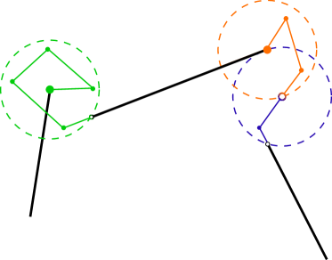
(a) This figure illustrates our partitioning of a curve into pieces (contained in dashed circles) and long segments (bold edges).

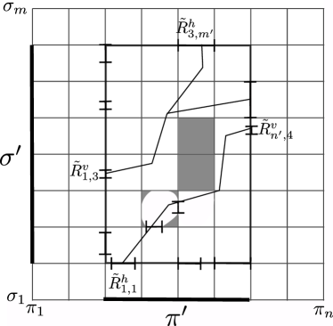
(b) The free-space problem for pieces $\pi^{\prime}$ and $\sigma^{\prime}$ in the free-space diagram of $\pi$ and $\sigma$. Given entry intervals on the lower and left boundary of the region, compute exit intervals on the upper and right boundary.

Figure 1: Definition and treatment of pieces.

Let $\pi,\sigma$ be curves for which we want to (approximately) decide whether $d_{\textup{F}}(\pi,\sigma)>\delta$ or $d_{\textup{F}}(\pi,\sigma)\leqslant(1+\varepsilon)\delta$. We modify the curve $\pi$ by introducing new vertices as follows. Start with the initial vertex $\pi_{1}$ as current vertex. If the segment following the current vertex has length at least $\Lambda=\Lambda_{\varepsilon,\delta}:=\operatorname{min}\{\tfrac{1}{2}\mathchoice{{\hbox{$\displaystyle\sqrt{\varepsilon\,}$}\lower 0.4pt\hbox{\vrule height=4.30554pt,depth=-3.44446pt}}}{{\hbox{$\textstyle\sqrt{\varepsilon\,}$}\lower 0.4pt\hbox{\vrule height=4.30554pt,depth=-3.44446pt}}}{{\hbox{$\scriptstyle\sqrt{\varepsilon\,}$}\lower 0.4pt\hbox{\vrule height=3.01389pt,depth=-2.41113pt}}}{{\hbox{$\scriptscriptstyle\sqrt{\varepsilon\,}$}\lower 0.4pt\hbox{\vrule height=2.15277pt,depth=-1.72223pt}}},\tfrac{1}{4}\}\cdot\delta$ then mark this segment as long and set the next vertex as the current vertex. Otherwise follow $\pi$ from the current vertex $\pi_{x}$ to the first point $\pi_{y}$ such that $\|\pi_{x}-\pi_{y}\|=\Lambda$ (or until we reach the last vertex of $\pi$). If $\pi_{y}$ is not a vertex, but lies on some segment of $\pi$, then introduce a new vertex at $\pi_{y}$. Mark $\pi_{x..y}$ as a piece of $\pi$ and set $\pi_{y}$ as current vertex. Repeat until $\pi$ is completely traversed. Since this procedure introduces at most $|\pi|$ new vertices and does not change the shape of $\pi$, with slight abuse of notation we call the resulting curve again $\pi$ and set $n:=|\pi|$. This partitions $\pi$ into subcurves $\pi^{1},\ldots,\pi^{k}$, with $\pi^{s}=\pi_{p_{s}..b_{s}}$, where every part $\pi^{s}$ is either (see also Figure 1a)

• a long segment: $b_{s}=p_{s}+1$ and $\|\pi_{p_{s}}-\pi_{b_{s}}\|\geqslant\Lambda$, or

• a piece: $\|\pi_{p_{s}}-\pi_{b_{s}}\|=\Lambda$ and $\|\pi_{p_{s}}-\pi_{x}\|<\Lambda$ for all $x\in[p_{s},b_{s})$.

Note that the last piece actually might have distance $\|\pi_{p_{s}}-\pi_{b_{s}}\|$ less than $\Lambda$, however, for simplicity we assume equality for all pieces (in fact, a special handling of the last piece would only be necessary in Lemma 3.6). Similarly, we introduce new vertices on $\sigma$ and partition it into subcurves $\sigma^{1},\ldots,\sigma^{\ell}$, with $\sigma^{t}=\sigma_{q_{t}..d_{t}}$, each of which is a long segment or a piece. Let $m:=|\sigma|$.

We do not want to resolve each free-space cell on its own, as in the standard decision algorithm for the Fréchet distance. Instead, for any pair of pieces we want to consider the free-space region spanned by the two pieces at once, see Figure 1b. This is made formal by the following subproblem.

Problem 3.1 (Free-space region problem).

Given $\delta>0$, $0<\varepsilon\leqslant 1$, curves $\pi,\sigma$ with $n$ and $m$ vertices, and entry intervals $\tilde{R}^{h}_{i,1}\subseteq[i,i+1]\times\{1\}$ for $i\in[1..n)$ and $\tilde{R}^{v}_{1,j}\subseteq\{1\}\times[j,j+1]$ for $j\in[1..m)$, compute exit intervals $\tilde{R}^{h}_{i,m}\subseteq[i,i+1]\times\{m\}$ for $i\in[1..n)$ and $\tilde{R}^{v}_{n,j}\subseteq\{n\}\times[j,j+1]$ for $j\in[1..m)$ such that (1) the exit intervals contain all points reachable from the entry intervals by a monotone path in $\mathcal{D}_{\leqslant\delta}(\pi,\sigma)$ and (2) all points in the exit intervals are reachable from the entry intervals by a monotone path in $\mathcal{D}_{\leqslant(1+\varepsilon)\delta}(\pi,\sigma)$.

To stress that we work with approximations, we denote reachable intervals by $\tilde{R}$ instead of $R$ in the remainder of the paper.

The standard solution to the free-space region problem would split it up into $n\cdot m$ free-space cells and resolve each cell in constant time, resulting in an $\mathcal{O}(n\cdot m)$ algorithm (this solves the problem even exactly, i.e., for $\varepsilon=0$). Restricted to pieces, we will show the following improvement, which will yield the desired overall speedup of a factor of $\textstyle\sqrt{\varepsilon\,}$ .

Lemma 3.2.

If $\pi$ and $\sigma$ are pieces then the free-space region problem can be solved in time $\mathcal{O}((n+m)\log^{2}1/\varepsilon)$.

We will prove this lemma in Sections 3.3 and 4.

Algorithm 3.3.

Using an algorithm for the free-space region problem on pieces as in Lemma 3.2, we obtain an approximate decider for the Fréchet distance a follows. We create a directed graph which has a node $v_{s,t}$ for every region $[p_{s},b_{s}]\times[q_{t},d_{t}]$ spanned by pieces $\pi^{s}$ and $\sigma^{t}$, and a node $u_{i,j}$ for every remaining region $[i,i+1]\times[j,j+1]$ (which is not contained in any region spanned by two pieces), $i\in[1..n)$, $j\in[1..m)$. We add edges between two nodes whenever their regions touch (i.e., have a common interval $I$ on their boundary), and direct this edge from the region that is to the left or below $I$ to the other one. With each node $u_{i,j}$ we store the entry intervals $\tilde{R}^{h}_{i,j}$ and $\tilde{R}^{v}_{i,j}$, and with each node $v_{s,t}$ we store the entry intervals $\tilde{R}^{h}_{i,q_{t}}\subseteq[i,i+1]\times\{q_{t}\}$ for $i\in[p_{s}..b_{s})$ and $\tilde{R}^{v}_{p_{s},j}\subseteq\{p_{s}\}\times[j,j+1]$ for $j\in[q_{t}..d_{t})$. After correctly initializing the outer reachability intervals $\tilde{R}^{h}_{i,1}$ and $\tilde{R}^{v}_{1,j}$, we follow any topological ordering of this graph. For any node $u_{i,j}$, we resolve its region by solving the corresponding free-space cell problem in constant time. For any node $v_{s,t}$, we solve the corresponding free-space region problem on $\pi^{\prime}=\pi^{s},\sigma^{\prime}=\sigma^{t}$ (and $\delta^{\prime}=\delta,\varepsilon^{\prime}=\varepsilon$) using Lemma 3.2. Finally, we return $d_{\textup{F}}(\pi,\sigma)\leqslant(1+\varepsilon)\delta$ if $(n,m)\in\tilde{R}^{h}_{n-1,m}$ and $d_{\textup{F}}(\pi,\sigma)>\delta$ otherwise.

Lemma 3.4.

Algorithm 3.3 is a correct approximate decider.

Proof.

Observe that if $(n,m)\in\tilde{R}^{h}_{n-1,m}$ then there exists a monotone path from $(1,1)$ to $(n,m)$ in $\mathcal{D}_{\leqslant(1+\varepsilon)\delta}(\pi,\sigma)$, which implies $d_{\textup{F}}(\pi,\sigma)\leqslant(1+\varepsilon)\delta$. If $d_{\textup{F}}(\pi,\sigma)\leqslant\delta$ then there is a monotone path from $(1,1)$ to $(n,m)$ in $\mathcal{D}_{\leqslant\delta}(\pi,\sigma)$, implying $(n,m)\in\tilde{R}^{h}_{n-1,m}$. ∎

In the above algorithm we can ignore unreachable nodes, i.e., nodes where all stored entry intervals would be empty. To this end, we fix a topological ordering by mapping a node corresponding to a region $[x_{1},x_{2}]\times[y_{1},y_{2}]$ to $x_{2}+y_{2}$ and sorting by this value ascendingly. This yields $n+m$ layers of nodes, where the order within each layer is arbitrary. For each layer we build a dictionary data structure (a hash table), in which we store only the reachable nodes of this layer. This allows to quickly enumerate all reachable nodes of a layer. The total overhead for managing the $n+m$ dictionaries is $\mathcal{O}(n+m)$.

Let us analyze the runtime of the obtained approximate decider. Let $S$ be the set of non-empty free-space cells $C_{i,j}$ of $\mathcal{D}_{\leqslant(1+\varepsilon)\delta}(\pi,\sigma)$ such that $i$ or $j$ is not contained in a piece. Moreover, let $T$ be the set of all pairs $(s,t)$ such that $\pi^{s},\sigma^{t}$ are pieces with initial vertices within distance $(1+\varepsilon)\delta+2\Lambda$. Define $N(\pi,\sigma,\delta,\varepsilon):=|S|+\sum_{(s,t)\in T}(|\pi^{s}|+|\sigma^{t}|)$ and set $N(\pi,\sigma,\varepsilon):=\operatorname{max}_{\delta>0}N(\pi,\sigma,\delta,\varepsilon)$. Since the algorithm considers only reachable cells and any reachable cell is also non-empty, the cost over all free-space cell problems solved by our approximate decider is bounded by $\mathcal{O}(|S|)$. Since every reachable (thus non-empty) region spanned by two pieces has initial points within distance $(1+\varepsilon)\delta+2\Lambda$, the second term bounds the cost over all free-space region problems on pieces (apart from the $\log^{2}1/\varepsilon$ factor). Hence, we obtain the following.

Lemma 3.5.

The approximate decider has runtime $D(\pi,\sigma,\varepsilon)=\mathcal{O}(N(\pi,\sigma,\varepsilon)\cdot\log^{2}1/\varepsilon)$.

3.1 The free-space complexity of $c$-packed curves

Recall that a curve $\pi$ is $c$-packed if for any point $z\in\mathbb{R}^{d}$ and any radius $r>0$ the total length of $\pi$ inside the ball $B(z,r)$ is at most $cr$.

Lemma 3.6.

Let $\pi,\sigma$ be $c$-packed curves with $n$ vertices in total and $\varepsilon>0$. Then $N(\pi,\sigma,\varepsilon)=\mathcal{O}(cn/\mathchoice{{\hbox{$\displaystyle\sqrt{\varepsilon\,}$}\lower 0.4pt\hbox{\vrule height=4.30554pt,depth=-3.44446pt}}}{{\hbox{$\textstyle\sqrt{\varepsilon\,}$}\lower 0.4pt\hbox{\vrule height=4.30554pt,depth=-3.44446pt}}}{{\hbox{$\scriptstyle\sqrt{\varepsilon\,}$}\lower 0.4pt\hbox{\vrule height=3.01389pt,depth=-2.41113pt}}}{{\hbox{$\scriptscriptstyle\sqrt{\varepsilon\,}$}\lower 0.4pt\hbox{\vrule height=2.15277pt,depth=-1.72223pt}}})$.

Proof.

Our proof uses a similar argument as [16, Lemma 4.4]. Let $\delta>0$ be arbitrary. First consider the set $S$ of non-empty free-space cells $C_{i,j}$ of $\mathcal{D}_{\leqslant(1+\varepsilon)\delta}(\pi,\sigma)$ such that $i$ or $j$ is not contained in a piece. Then one of the segments $\pi_{i..i+1}$ and $\sigma_{j..j+1}$ is long, i.e., of length at least $\Lambda=\operatorname{min}\{\tfrac{1}{2}\mathchoice{{\hbox{$\displaystyle\sqrt{\varepsilon\,}$}\lower 0.4pt\hbox{\vrule height=4.30554pt,depth=-3.44446pt}}}{{\hbox{$\textstyle\sqrt{\varepsilon\,}$}\lower 0.4pt\hbox{\vrule height=4.30554pt,depth=-3.44446pt}}}{{\hbox{$\scriptstyle\sqrt{\varepsilon\,}$}\lower 0.4pt\hbox{\vrule height=3.01389pt,depth=-2.41113pt}}}{{\hbox{$\scriptscriptstyle\sqrt{\varepsilon\,}$}\lower 0.4pt\hbox{\vrule height=2.15277pt,depth=-1.72223pt}}},\tfrac{1}{4}\}\cdot\delta$. We charge the cell $C_{i,j}$ to the shorter of the two segments. Let us analyze how often any segment $v=\pi_{i..i+1}$ can be charged. Consider the ball $B$ of radius $r:=\tfrac{1}{2}\|v\|+(1+\varepsilon)\delta+\operatorname{max}\{\|v\|,\Lambda\}$ centered at the midpoint of $v$. Every segment $u=\sigma_{j..j+1}$ with $(i,j)\in S$, which charges $v$, is of length at least $\mu:=\operatorname{max}\{\|v\|,\Lambda\}$ (since it is longer than $v$ and a long segment) and contributes at least $\mu$ to the total length of $\sigma$ in $B$. Since $\sigma$ is $c$-packed, the number of such charges is at most

$$\frac{\|\sigma\cap B\|}{\mu}\leqslant\frac{cr}{\mu}\leqslant\frac{c(\tfrac{1}{2}\|v\|+(1+\varepsilon)\delta+\operatorname{max}\{\|v\|,\Lambda\})}{\operatorname{max}\{\|v\|,\Lambda\}}\leqslant\tfrac{3}{2}c+\frac{c(1+\varepsilon)\delta}{\operatorname{min}\{\tfrac{1}{2}\mathchoice{{\hbox{$\displaystyle\sqrt{\varepsilon\,}$}\lower 0.4pt\hbox{\vrule height=4.30554pt,depth=-3.44446pt}}}{{\hbox{$\textstyle\sqrt{\varepsilon\,}$}\lower 0.4pt\hbox{\vrule height=4.30554pt,depth=-3.44446pt}}}{{\hbox{$\scriptstyle\sqrt{\varepsilon\,}$}\lower 0.4pt\hbox{\vrule height=3.01389pt,depth=-2.41113pt}}}{{\hbox{$\scriptscriptstyle\sqrt{\varepsilon\,}$}\lower 0.4pt\hbox{\vrule height=2.15277pt,depth=-1.72223pt}}},\tfrac{1}{4}\}\cdot\delta}=\mathcal{O}\Big{(}\frac{c}{\mathchoice{{\hbox{$\displaystyle\sqrt{\varepsilon\,}$}\lower 0.4pt\hbox{\vrule height=4.30554pt,depth=-3.44446pt}}}{{\hbox{$\textstyle\sqrt{\varepsilon\,}$}\lower 0.4pt\hbox{\vrule height=4.30554pt,depth=-3.44446pt}}}{{\hbox{$\scriptstyle\sqrt{\varepsilon\,}$}\lower 0.4pt\hbox{\vrule height=3.01389pt,depth=-2.41113pt}}}{{\hbox{$\scriptscriptstyle\sqrt{\varepsilon\,}$}\lower 0.4pt\hbox{\vrule height=2.15277pt,depth=-1.72223pt}}}}\Big{)}.$$

Thus, the contribution of $|S|$ to the free-space complexity $N(\pi,\sigma,\varepsilon)$ is $\mathcal{O}(cn/\mathchoice{{\hbox{$\displaystyle\sqrt{\varepsilon\,}$}\lower 0.4pt\hbox{\vrule height=4.30554pt,depth=-3.44446pt}}}{{\hbox{$\textstyle\sqrt{\varepsilon\,}$}\lower 0.4pt\hbox{\vrule height=4.30554pt,depth=-3.44446pt}}}{{\hbox{$\scriptstyle\sqrt{\varepsilon\,}$}\lower 0.4pt\hbox{\vrule height=3.01389pt,depth=-2.41113pt}}}{{\hbox{$\scriptscriptstyle\sqrt{\varepsilon\,}$}\lower 0.4pt\hbox{\vrule height=2.15277pt,depth=-1.72223pt}}})$.

Let $T$ be the set of all pairs $(s,t)$ such that $\pi^{s},\sigma^{t}$ are pieces of $\pi,\sigma$ with initial vertices within distance $(1+\varepsilon)\delta+2\Lambda$, and consider $\Sigma:=\sum_{(s,t)\in T}(|\pi^{s}|+|\sigma^{t}|)$. We distribute $\Sigma$ over the segments of $\pi,\sigma$ by charging 1 to every segment of $\pi^{s}$ and $\sigma^{t}$ for any pair $(s,t)\in T$. Let us analyze how often any segment $v$ of a piece $\pi^{s}$ can be charged. Consider the ball $B^{\prime}$ of radius $r^{\prime}:=(1+\varepsilon)\delta+3\Lambda$ around the initital vertex $\pi_{p_{s}}$ of $\pi^{s}$. Since $\|\sigma^{t}\|\geqslant\Lambda$, for any $(s,t)\in T$ the piece $\sigma^{t}$ contributes at least $\Lambda$ to the total length of $\sigma$ in $B^{\prime}$. Since $\sigma$ is $c$-packed, the number of such charges to $v$ is at most

$$\frac{\|\sigma\cap B^{\prime}\|}{\Lambda}\leqslant\frac{cr^{\prime}}{\Lambda}=\frac{c(1+\varepsilon+\tfrac{3}{2}\mathchoice{{\hbox{$\displaystyle\sqrt{\varepsilon\,}$}\lower 0.4pt\hbox{\vrule height=4.30554pt,depth=-3.44446pt}}}{{\hbox{$\textstyle\sqrt{\varepsilon\,}$}\lower 0.4pt\hbox{\vrule height=4.30554pt,depth=-3.44446pt}}}{{\hbox{$\scriptstyle\sqrt{\varepsilon\,}$}\lower 0.4pt\hbox{\vrule height=3.01389pt,depth=-2.41113pt}}}{{\hbox{$\scriptscriptstyle\sqrt{\varepsilon\,}$}\lower 0.4pt\hbox{\vrule height=2.15277pt,depth=-1.72223pt}}})}{\operatorname{min}\{\tfrac{1}{2}\mathchoice{{\hbox{$\displaystyle\sqrt{\varepsilon\,}$}\lower 0.4pt\hbox{\vrule height=4.30554pt,depth=-3.44446pt}}}{{\hbox{$\textstyle\sqrt{\varepsilon\,}$}\lower 0.4pt\hbox{\vrule height=4.30554pt,depth=-3.44446pt}}}{{\hbox{$\scriptstyle\sqrt{\varepsilon\,}$}\lower 0.4pt\hbox{\vrule height=3.01389pt,depth=-2.41113pt}}}{{\hbox{$\scriptscriptstyle\sqrt{\varepsilon\,}$}\lower 0.4pt\hbox{\vrule height=2.15277pt,depth=-1.72223pt}}},\tfrac{1}{4}\}}=\mathcal{O}\Big{(}\frac{c}{\mathchoice{{\hbox{$\displaystyle\sqrt{\varepsilon\,}$}\lower 0.4pt\hbox{\vrule height=4.30554pt,depth=-3.44446pt}}}{{\hbox{$\textstyle\sqrt{\varepsilon\,}$}\lower 0.4pt\hbox{\vrule height=4.30554pt,depth=-3.44446pt}}}{{\hbox{$\scriptstyle\sqrt{\varepsilon\,}$}\lower 0.4pt\hbox{\vrule height=3.01389pt,depth=-2.41113pt}}}{{\hbox{$\scriptscriptstyle\sqrt{\varepsilon\,}$}\lower 0.4pt\hbox{\vrule height=2.15277pt,depth=-1.72223pt}}}}\Big{)}.$$

Hence, the contribution of $\Sigma$ to the free-space complexity $N(\pi,\sigma,\varepsilon)$ is also at most $\mathcal{O}(cn/\mathchoice{{\hbox{$\displaystyle\sqrt{\varepsilon\,}$}\lower 0.4pt\hbox{\vrule height=4.30554pt,depth=-3.44446pt}}}{{\hbox{$\textstyle\sqrt{\varepsilon\,}$}\lower 0.4pt\hbox{\vrule height=4.30554pt,depth=-3.44446pt}}}{{\hbox{$\scriptstyle\sqrt{\varepsilon\,}$}\lower 0.4pt\hbox{\vrule height=3.01389pt,depth=-2.41113pt}}}{{\hbox{$\scriptscriptstyle\sqrt{\varepsilon\,}$}\lower 0.4pt\hbox{\vrule height=2.15277pt,depth=-1.72223pt}}})$, which finishes the proof. ∎

Combining Lemmas 3.6, 3.5, and 2.1, we obtain an approximation algorithm for the Fréchet distance with running time $\mathcal{O}(\tfrac{cn}{\mathchoice{{\hbox{$\displaystyle\sqrt{\varepsilon\,}$}\lower 0.4pt\hbox{\vrule height=3.01389pt,depth=-2.41113pt}}}{{\hbox{$\textstyle\sqrt{\varepsilon\,}$}\lower 0.4pt\hbox{\vrule height=3.01389pt,depth=-2.41113pt}}}{{\hbox{$\scriptstyle\sqrt{\varepsilon\,}$}\lower 0.4pt\hbox{\vrule height=2.10971pt,depth=-1.68779pt}}}{{\hbox{$\scriptscriptstyle\sqrt{\varepsilon\,}$}\lower 0.4pt\hbox{\vrule height=1.50694pt,depth=-1.20557pt}}}}\log^{2}1/\varepsilon+cn\log n)=\tilde{\mathcal{O}}(\tfrac{cn}{\mathchoice{{\hbox{$\displaystyle\sqrt{\varepsilon\,}$}\lower 0.4pt\hbox{\vrule height=3.01389pt,depth=-2.41113pt}}}{{\hbox{$\textstyle\sqrt{\varepsilon\,}$}\lower 0.4pt\hbox{\vrule height=3.01389pt,depth=-2.41113pt}}}{{\hbox{$\scriptstyle\sqrt{\varepsilon\,}$}\lower 0.4pt\hbox{\vrule height=2.10971pt,depth=-1.68779pt}}}{{\hbox{$\scriptscriptstyle\sqrt{\varepsilon\,}$}\lower 0.4pt\hbox{\vrule height=1.50694pt,depth=-1.20557pt}}}})$, as desired.

3.2 The free-space complexity of $\kappa$-bounded and $\kappa$-straight curves

Definition 3.7.

Let $\kappa\geqslant 1$ be a given parameter. A curve $\pi$ is $\kappa$-straight if for any $p,b\in[1,|\pi|]$ we have $\|\pi_{p..b}\|\leqslant\kappa\|\pi_{p}-\pi_{b}\|$. A curve $\pi$ is $\kappa$-bounded if for all $p,b$ the subcurve $\pi_{p..b}$ is contained in $B(\pi_{p},r)\cup B(\pi_{b},r)$, where $r=\tfrac{\kappa}{2}\|\pi_{p}-\pi_{b}\|$.

The following lemma from [16] allows us to transfer our speedup for $c$-packed curves directly to $\kappa$-straight curves.

Lemma 3.8.

A $\kappa$-straight curve is $2\kappa$-packed.

In the remainder of this section we consider $\kappa$-bounded curves, closely following [16, Sect. 4.2].

Lemma 3.9.

Let $\delta>0$, $0<\varepsilon\leqslant 1$, $\lambda>0$, and let $\pi$ be a $\kappa$-bounded curve with disjoint subcurves $\pi^{1},\ldots,\pi^{k}$, where $\pi^{s}=\pi_{p_{s}..b_{s}}$ and $\|\pi_{p_{s}}-\pi_{b_{s}}\|\geqslant\lambda$ for all $s$. Then for any $z\in\mathbb{R}^{d}$, $r>0$ the number of subcurves $\pi^{s}$ intersecting $B(z,r)$ is bounded by $\mathcal{O}(\kappa^{d}(1+r/\lambda)^{d})$.

Proof.

Let $\pi^{s_{1}},\ldots,\pi^{s_{\ell}}$ be the subcurves that intersect the ball $B=B(z,r)$. Let $X=\{s_{1},s_{3},\ldots,\}$ be the odd indices among the intersecting subcurves. For all $s\in X$ pick any point $\pi_{x_{s}}$ in $\pi^{s}\cap B$. Between any points $\pi_{x_{s}},\pi_{x_{s^{\prime}}}$ there must lie an even subcurve $\pi^{s_{2i}}$. As the endpoints of this even subcurve have distance at least $\lambda$, we have $\|\pi_{x_{s}}-\pi_{x_{s^{\prime}}}\|\geqslant\lambda/(\kappa+1)$. Otherwise the even part would not fit into $B(\pi_{x_{s}},r)\cup B(\pi_{x_{s^{\prime}}},r)$ which has diameter $(\kappa+1)\|\pi_{x_{s}}-\pi_{x_{s^{\prime}}}\|$. Hence, the balls $B(\pi_{x_{s}},\lambda/2(\kappa+1))$ are disjoint and contained in $B(z,r+\lambda)$. A standard packing argument now shows that $\ell\leqslant 2\cdot(r+\lambda)^{d}/(\lambda/2(\kappa+1))^{d}=\mathcal{O}(\kappa^{d}(1+r/\lambda)^{d})$. ∎

Lemma 3.10.

For any $\kappa$-bounded curves $\pi,\sigma$ with $n$ vertices in total, $0<\varepsilon\leqslant 1$, we have $N(\pi,\sigma,\varepsilon)=\mathcal{O}((\kappa/\mathchoice{{\hbox{$\displaystyle\sqrt{\varepsilon\,}$}\lower 0.4pt\hbox{\vrule height=4.30554pt,depth=-3.44446pt}}}{{\hbox{$\textstyle\sqrt{\varepsilon\,}$}\lower 0.4pt\hbox{\vrule height=4.30554pt,depth=-3.44446pt}}}{{\hbox{$\scriptstyle\sqrt{\varepsilon\,}$}\lower 0.4pt\hbox{\vrule height=3.01389pt,depth=-2.41113pt}}}{{\hbox{$\scriptscriptstyle\sqrt{\varepsilon\,}$}\lower 0.4pt\hbox{\vrule height=2.15277pt,depth=-1.72223pt}}})^{d}n)$.

Proof.

Let $\delta>0$ and consider the partitionings into long segments and pieces $\pi^{1},\ldots,\pi^{k}$, $\sigma^{1},\ldots,\sigma^{\ell}$ computed by our algorithm. Then $\sigma^{t}=\sigma_{q_{t}..d_{t}}$ satisfies $\|\sigma_{q_{t}}-\sigma_{d_{t}}\|\geqslant\Lambda=\operatorname{min}\{\tfrac{1}{2}\mathchoice{{\hbox{$\displaystyle\sqrt{\varepsilon\,}$}\lower 0.4pt\hbox{\vrule height=4.30554pt,depth=-3.44446pt}}}{{\hbox{$\textstyle\sqrt{\varepsilon\,}$}\lower 0.4pt\hbox{\vrule height=4.30554pt,depth=-3.44446pt}}}{{\hbox{$\scriptstyle\sqrt{\varepsilon\,}$}\lower 0.4pt\hbox{\vrule height=3.01389pt,depth=-2.41113pt}}}{{\hbox{$\scriptscriptstyle\sqrt{\varepsilon\,}$}\lower 0.4pt\hbox{\vrule height=2.15277pt,depth=-1.72223pt}}},\tfrac{1}{4}\}\cdot\delta$ for all $t$. We use the same charging scheme as in Lemma 3.6. Consider any segment $v$ of a piece $\pi^{s}$. The segment $v$ can be charged by a part $\sigma^{t}$ which is either a long segment or a piece. In both cases, $\sigma^{t}$ intersects the ball $B$ centered at the midpoint of $\|v\|$ with radius $r:=(1+\varepsilon)\delta+2\Lambda$. By Lemma 3.9 with $\lambda:=\Lambda$, the number of such charges is bounded by $\mathcal{O}((\kappa/\mathchoice{{\hbox{$\displaystyle\sqrt{\varepsilon\,}$}\lower 0.4pt\hbox{\vrule height=4.30554pt,depth=-3.44446pt}}}{{\hbox{$\textstyle\sqrt{\varepsilon\,}$}\lower 0.4pt\hbox{\vrule height=4.30554pt,depth=-3.44446pt}}}{{\hbox{$\scriptstyle\sqrt{\varepsilon\,}$}\lower 0.4pt\hbox{\vrule height=3.01389pt,depth=-2.41113pt}}}{{\hbox{$\scriptscriptstyle\sqrt{\varepsilon\,}$}\lower 0.4pt\hbox{\vrule height=2.15277pt,depth=-1.72223pt}}})^{d})$.

Now consider any long segment $v$ of $\pi$. The segment $v$ can be charged by segments of $\sigma$ which are longer than $v$. Any such charging gives rise to a long segment $\sigma^{t}$ intersecting the ball $B$ centered at the midpoint of $v$ of radius $r:=(1+\varepsilon)\delta+\tfrac{1}{2}\|v\|$. By Lemma 3.9 with $\lambda:=\|v\|$, the number of such charges is bounded by $\mathcal{O}(\kappa^{d}(\tfrac{3}{2}+(1+\varepsilon)\delta/\|v\|)^{d})=\mathcal{O}((\kappa/\mathchoice{{\hbox{$\displaystyle\sqrt{\varepsilon\,}$}\lower 0.4pt\hbox{\vrule height=4.30554pt,depth=-3.44446pt}}}{{\hbox{$\textstyle\sqrt{\varepsilon\,}$}\lower 0.4pt\hbox{\vrule height=4.30554pt,depth=-3.44446pt}}}{{\hbox{$\scriptstyle\sqrt{\varepsilon\,}$}\lower 0.4pt\hbox{\vrule height=3.01389pt,depth=-2.41113pt}}}{{\hbox{$\scriptscriptstyle\sqrt{\varepsilon\,}$}\lower 0.4pt\hbox{\vrule height=2.15277pt,depth=-1.72223pt}}})^{d})$, since $\|v\|\geqslant\Lambda=\operatorname{min}\{\tfrac{1}{2}\mathchoice{{\hbox{$\displaystyle\sqrt{\varepsilon\,}$}\lower 0.4pt\hbox{\vrule height=4.30554pt,depth=-3.44446pt}}}{{\hbox{$\textstyle\sqrt{\varepsilon\,}$}\lower 0.4pt\hbox{\vrule height=4.30554pt,depth=-3.44446pt}}}{{\hbox{$\scriptstyle\sqrt{\varepsilon\,}$}\lower 0.4pt\hbox{\vrule height=3.01389pt,depth=-2.41113pt}}}{{\hbox{$\scriptscriptstyle\sqrt{\varepsilon\,}$}\lower 0.4pt\hbox{\vrule height=2.15277pt,depth=-1.72223pt}}},\tfrac{1}{4}\}\cdot\delta$.

Hence, every segment of $\pi$ is charged $\mathcal{O}((\kappa/\mathchoice{{\hbox{$\displaystyle\sqrt{\varepsilon\,}$}\lower 0.4pt\hbox{\vrule height=4.30554pt,depth=-3.44446pt}}}{{\hbox{$\textstyle\sqrt{\varepsilon\,}$}\lower 0.4pt\hbox{\vrule height=4.30554pt,depth=-3.44446pt}}}{{\hbox{$\scriptstyle\sqrt{\varepsilon\,}$}\lower 0.4pt\hbox{\vrule height=3.01389pt,depth=-2.41113pt}}}{{\hbox{$\scriptscriptstyle\sqrt{\varepsilon\,}$}\lower 0.4pt\hbox{\vrule height=2.15277pt,depth=-1.72223pt}}})^{d})$ times; a symmetric statement holds for $\sigma$. ∎

Plugging the above lemma into Lemma 2.1 we obtain the following result. The best previously known runtime was $\mathcal{O}((\kappa/\varepsilon)^{d}n+\kappa^{d}n\log n)$ [16].

Theorem 3.11.

For any $0<\varepsilon\leqslant 1$ there is a $(1+\varepsilon)$-approximation for the continuous and discrete Fréchet distance on $\kappa$-bounded curves with $n$ vertices in total in time $\mathcal{O}((\kappa/\mathchoice{{\hbox{$\displaystyle\sqrt{\varepsilon\,}$}\lower 0.4pt\hbox{\vrule height=4.30554pt,depth=-3.44446pt}}}{{\hbox{$\textstyle\sqrt{\varepsilon\,}$}\lower 0.4pt\hbox{\vrule height=4.30554pt,depth=-3.44446pt}}}{{\hbox{$\scriptstyle\sqrt{\varepsilon\,}$}\lower 0.4pt\hbox{\vrule height=3.01389pt,depth=-2.41113pt}}}{{\hbox{$\scriptscriptstyle\sqrt{\varepsilon\,}$}\lower 0.4pt\hbox{\vrule height=2.15277pt,depth=-1.72223pt}}})^{d}n\log^{2}1/\varepsilon+\kappa^{d}n\log n)=\tilde{\mathcal{O}}((\kappa/\mathchoice{{\hbox{$\displaystyle\sqrt{\varepsilon\,}$}\lower 0.4pt\hbox{\vrule height=4.30554pt,depth=-3.44446pt}}}{{\hbox{$\textstyle\sqrt{\varepsilon\,}$}\lower 0.4pt\hbox{\vrule height=4.30554pt,depth=-3.44446pt}}}{{\hbox{$\scriptstyle\sqrt{\varepsilon\,}$}\lower 0.4pt\hbox{\vrule height=3.01389pt,depth=-2.41113pt}}}{{\hbox{$\scriptscriptstyle\sqrt{\varepsilon\,}$}\lower 0.4pt\hbox{\vrule height=2.15277pt,depth=-1.72223pt}}})^{d}n)$.

3.3 Solving the free-space region problem on pieces

It remains to prove Lemma 3.2. Let $(\pi,\sigma,\delta,\varepsilon)$ be an instance of the free-space region problem, where $n:=|\pi|$, $m:=|\sigma|$, with $\|\pi_{1}-\pi_{x}\|,\|\sigma_{1}-\sigma_{y}\|\leqslant\Lambda_{\varepsilon,\delta}=\Lambda$ for any $x\in[1,n]$, $y\in[1,m]$ (and entry intervals $\tilde{R}^{h}_{i,1}\subseteq[i,i+1]\times\{1\}$ for $i\in[1..n)$ and $\tilde{R}^{v}_{1,j}\subseteq\{1\}\times[j,j+1]$ for $j\in[1..m)$). We reduce this instance to the free-space region problem on one-dimensional separated curves, i.e., curves $\hat{\pi},\hat{\sigma}$ in $\mathbb{R}$ such that all vertices of $\hat{\pi}$ lie above 0 and all vertices of $\hat{\sigma}$ lie below 0.

Since $\pi$ and $\sigma$ stay within distance $\Lambda$ of their initial vertices, if their initial vertices are within distance $\|\pi_{1}-\sigma_{1}\|\leqslant\delta-2\Lambda$ then all pairs of points in $\pi,\sigma$ are within distance $\delta$. In this case, we find a translation of $\pi$ making $\|\pi_{1}-\sigma_{1}\|=\delta-2\Lambda$ and all pairwise distances are still at most $\delta$. This ensures that the curves $\pi,\sigma$ are contained in disjoint balls of radius $\Lambda\leqslant\tfrac{1}{4}\delta$ centered at their initial vertices.

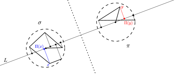
Figure 2: Projection of the pieces $\pi,\sigma$ onto the line $L$ through their initial vertices. This yields one-dimensional separated curves $\hat{\pi},\hat{\sigma}$.

Consider the line $L$ through the initial vertices $\pi_{1}$ and $\sigma_{1}$. Denote by $\Pi\colon\mathbb{R}^{d}\to L$ the projection onto $L$. Now, instead of the pieces $\pi,\sigma$ we consider their projections $\hat{\pi}:=\Pi(\pi)=(\Pi(\pi_{1}),\ldots,\Pi(\pi_{n}))$ and $\hat{\sigma}:=\Pi(\sigma)=(\Pi(\sigma_{1}),\ldots,\Pi(\sigma_{m}))$, see Figure 2. Note that after rotation and translation we can assume that $\hat{\pi}$ and $\hat{\sigma}$ lie on $\mathbb{R}\subset\mathbb{R}^{d}$ and $\hat{\pi}$ and $\hat{\sigma}$ are separated by $0\in\mathbb{R}$ (since $\pi$ and $\sigma$ are contained in disjoined balls centered on $L$). Now we solve the free-space region problem on $\hat{\pi}$, $\hat{\sigma}$, $\hat{\delta}:=\delta$, and $\hat{}\varepsilon:=\tfrac{1}{2}\varepsilon$ (with the same entry intervals $\tilde{R}^{h}_{i,j},\tilde{R}^{v}_{i,j})$).

Lemma 3.12.

Any solution to the the free-space region problem on $(\hat{\pi},\hat{\sigma},\hat{\delta},\hat{}\varepsilon)$ solves the free-space region problem on $(\pi,\sigma,\delta,\varepsilon)$.

Proof.

Let $x,y$ be vertices of $\pi,\sigma$, respectively. Clearly, $\|\Pi(x)-\Pi(y)\|\leqslant\|x-y\|$. Hence, any monotone path in $\mathcal{D}_{\leqslant\delta}(\pi,\sigma)$ yields a monotone path in $\mathcal{D}_{\leqslant\delta}(\hat{\pi},\hat{\sigma})=\mathcal{D}_{\leqslant\hat{\delta}}(\hat{\pi},\hat{\sigma})$, so it will be found.

Note that $x$ and $y$ have distance at most $\Lambda$ to $L$. Since $\Pi(x)-\Pi(y)$ and $x-\Pi(x)-(y-\Pi(y))$ are orthogonal, we can use the Pythagorean theorem to obtain

$$\|x-y\|=\mathchoice{{\hbox{$\displaystyle\sqrt{\|\Pi(x)-\Pi(y)\|^{2}+\|x-\Pi(x)-(y-\Pi(y))\|^{2}\,}$}\lower 0.4pt\hbox{\vrule height=9.30444pt,depth=-7.44359pt}}}{{\hbox{$\textstyle\sqrt{\|\Pi(x)-\Pi(y)\|^{2}+\|x-\Pi(x)-(y-\Pi(y))\|^{2}\,}$}\lower 0.4pt\hbox{\vrule height=9.30444pt,depth=-7.44359pt}}}{{\hbox{$\scriptstyle\sqrt{\|\Pi(x)-\Pi(y)\|^{2}+\|x-\Pi(x)-(y-\Pi(y))\|^{2}\,}$}\lower 0.4pt\hbox{\vrule height=6.53888pt,depth=-5.23112pt}}}{{\hbox{$\scriptscriptstyle\sqrt{\|\Pi(x)-\Pi(y)\|^{2}+\|x-\Pi(x)-(y-\Pi(y))\|^{2}\,}$}\lower 0.4pt\hbox{\vrule height=5.03888pt,depth=-4.03113pt}}}\leqslant\mathchoice{{\hbox{$\displaystyle\sqrt{\|\Pi(x)-\Pi(y)\|^{2}+(2\Lambda)^{2}\,}$}\lower 0.4pt\hbox{\vrule height=9.30444pt,depth=-7.44359pt}}}{{\hbox{$\textstyle\sqrt{\|\Pi(x)-\Pi(y)\|^{2}+(2\Lambda)^{2}\,}$}\lower 0.4pt\hbox{\vrule height=9.30444pt,depth=-7.44359pt}}}{{\hbox{$\scriptstyle\sqrt{\|\Pi(x)-\Pi(y)\|^{2}+(2\Lambda)^{2}\,}$}\lower 0.4pt\hbox{\vrule height=6.53888pt,depth=-5.23112pt}}}{{\hbox{$\scriptscriptstyle\sqrt{\|\Pi(x)-\Pi(y)\|^{2}+(2\Lambda)^{2}\,}$}\lower 0.4pt\hbox{\vrule height=5.03888pt,depth=-4.03113pt}}}.$$

Hence, any monotone path in $\mathcal{D}_{\leqslant(1+\hat{}\varepsilon)\hat{\delta}}(\hat{\pi},\hat{\sigma})$ yields a monotone path in $\mathcal{D}_{\leqslant\alpha}(\pi,\sigma)$ with $\alpha\leqslant\mathchoice{{\hbox{$\displaystyle\sqrt{(1+\hat{}\varepsilon)^{2}\hat{\delta}^{2}+(2\Lambda)^{2}\,}$}\lower 0.4pt\hbox{\vrule height=9.30444pt,depth=-7.44359pt}}}{{\hbox{$\textstyle\sqrt{(1+\hat{}\varepsilon)^{2}\hat{\delta}^{2}+(2\Lambda)^{2}\,}$}\lower 0.4pt\hbox{\vrule height=9.30444pt,depth=-7.44359pt}}}{{\hbox{$\scriptstyle\sqrt{(1+\hat{}\varepsilon)^{2}\hat{\delta}^{2}+(2\Lambda)^{2}\,}$}\lower 0.4pt\hbox{\vrule height=8.51111pt,depth=-6.80891pt}}}{{\hbox{$\scriptscriptstyle\sqrt{(1+\hat{}\varepsilon)^{2}\hat{\delta}^{2}+(2\Lambda)^{2}\,}$}\lower 0.4pt\hbox{\vrule height=8.51111pt,depth=-6.80891pt}}}$. Plugging in $\hat{\delta}=\delta$, $\hat{}\varepsilon=\tfrac{1}{2}\varepsilon$, and $\Lambda=\operatorname{min}\{\tfrac{1}{2}\mathchoice{{\hbox{$\displaystyle\sqrt{\varepsilon\,}$}\lower 0.4pt\hbox{\vrule height=4.30554pt,depth=-3.44446pt}}}{{\hbox{$\textstyle\sqrt{\varepsilon\,}$}\lower 0.4pt\hbox{\vrule height=4.30554pt,depth=-3.44446pt}}}{{\hbox{$\scriptstyle\sqrt{\varepsilon\,}$}\lower 0.4pt\hbox{\vrule height=3.01389pt,depth=-2.41113pt}}}{{\hbox{$\scriptscriptstyle\sqrt{\varepsilon\,}$}\lower 0.4pt\hbox{\vrule height=2.15277pt,depth=-1.72223pt}}},\tfrac{1}{4}\}\cdot\delta$ we obtain $\alpha\leqslant\mathchoice{{\hbox{$\displaystyle\sqrt{(1+\tfrac{1}{2}\varepsilon)^{2}+\varepsilon\,}$}\lower 0.4pt\hbox{\vrule height=9.30444pt,depth=-7.44359pt}}}{{\hbox{$\textstyle\sqrt{(1+\tfrac{1}{2}\varepsilon)^{2}+\varepsilon\,}$}\lower 0.4pt\hbox{\vrule height=9.30444pt,depth=-7.44359pt}}}{{\hbox{$\scriptstyle\sqrt{(1+\tfrac{1}{2}\varepsilon)^{2}+\varepsilon\,}$}\lower 0.4pt\hbox{\vrule height=6.76666pt,depth=-5.41336pt}}}{{\hbox{$\scriptscriptstyle\sqrt{(1+\tfrac{1}{2}\varepsilon)^{2}+\varepsilon\,}$}\lower 0.4pt\hbox{\vrule height=6.76666pt,depth=-5.41336pt}}}\cdot\delta\leqslant(1+\varepsilon)\,\delta$. Thus, the desired guarantees for the free-space region problem are satisfied. ∎

We will show the following lemma in Section 4, concluding the proof of Lemma 3.2.

Lemma 3.13.

The free-space region problem on one-dimensional separated curves can be solved in time $\mathcal{O}((n+m)\log^{2}1/\varepsilon)$.

4 On one-dimensional separated curves

In this section, we show how to solve the free-space region problem on one-dimensional separated curves in time $\mathcal{O}((n+m)\log^{2}1/\varepsilon)$, i.e., we prove Lemma 3.13.

First, in Section 4.1, we show how to reduce this problem to a discrete version, meaning that we can eliminate the continuous Fréchet distance and only consider the much simpler discrete Fréchet distance (for general curves such a reduction is not known to exist, but we only need it for one-dimensional separated curves). Moreover, we simplify our curves further by rounding the vertices. This yields a reduction to the following subproblem. Note that we no longer ask for an approximation algorithm.

Problem 4.1 (Reduced free-space problem).

Given one-dimensional separated curves $\pi,\sigma$ with $n,m$ vertices and all vertices being multiples of $\tfrac{1}{3}\varepsilon\delta$, and given an entry set $E\subseteq[1..n]$, compute the exit set $F^{\pi}\subseteq[1..n]$ consisting of all points $f$ such that $d_{\textup{dF}}(\pi_{e..f},\sigma)\leqslant\delta$ for some $e\in E$ and the exit set $F^{\sigma}\subseteq[1..m]$ consisting of all points $f$ such that $d_{\textup{dF}}(\pi_{e..n},\sigma_{1..f})\leqslant\delta$ for some $e\in E$.

Lemma 4.2.

The reduced free-space problem can be solved in time $\mathcal{O}((n+m)\log 1/\varepsilon)$.

As a second step, we prove the above lemma. We first consider the special case of $E=\{1\}$ and the problem of deciding whether $n\in F^{\pi}$, i.e., the lower left corner $(1,1)$ of the free-space is the only entry point and we want to determine whether the upper right corner $(n,m)$ is an exit. This is equivalent to deciding whether the discrete Fréchet distance of $\pi,\sigma$ is at most $\delta$, which is known to have a near-linear time algorithm as $\pi,\sigma$ are one-dimensional and separated (see the footnote in the introduction for details). We present a greedy algorithm for this special case in Section 4.2. To extend this to the reduced free-space problem, we prove useful structural properties of one-dimensional separated curves in Section 4.3. With these, we first solve the problem of determining the exit set $F^{\pi}$ assuming $E=\{1\}$ in Section 4.4.1. Then we show for general $E\subseteq[1..n]$ how to compute $F^{\pi}$ (Section 4.4.2) and $F^{\sigma}$ (Section 4.4.3).

4.1 Reduction from the continuous to the discrete case

Essentially we use the following lemma to reduce the continuous free-space region problem on one-dimensional separated curves to the discrete reduced free-space problem.

Lemma 4.3.

Let $\pi,\sigma$ be one-dimensional separated curves with subcurves $\pi_{p..b},\sigma_{q..d}$. Then we have $d_{\textup{F}}(\pi_{p..b},\sigma_{q..d})=d_{\textup{dF}}(\pi_{p..b},\sigma_{q..d})$. In particular, assume that we subdivide any segments of $\pi,\sigma$ by adding new vertices, which yields new curves $\pi^{\prime},\sigma^{\prime}$ with subcurves $\pi^{\prime}_{p^{\prime}..b^{\prime}},\sigma^{\prime}_{q^{\prime}..d^{\prime}}$ that are subdivisions of $\pi_{p..b},\sigma_{q..d}$. Then we have $d_{\textup{dF}}(\pi^{\prime}_{p^{\prime}..b^{\prime}},\sigma^{\prime}_{q^{\prime}..d^{\prime}})=d_{\textup{dF}}(\pi_{p..b},\sigma_{q..d})=d_{\textup{F}}(\pi_{p..b},\sigma_{q..d})$.

Proof.

It is known that $d_{\textup{F}}(\pi,\sigma)\leqslant d_{\textup{dF}}(\pi,\sigma)$ holds for all curves $\pi,\sigma$. Thus, we only need to show that any continuous traversal $\phi=(\phi_{1},\phi_{2})$ of $\pi_{p..b},\sigma_{q..d}$ can be transformed into a discrete traversal with the same width. We adapt $\phi$ as follows. For any point in time $t\in[0,1]$, if $\phi_{1}(t)$ is at a vertex of $\pi$ we set $\phi^{\prime}_{1}(t):=\phi_{1}(t)$. Otherwise $\phi_{1}(t)$ is in the interior of a segment $\pi_{i..i+1}$ of $\pi$. Let $j\in\{i,i+1\}$ minimize $\pi_{j}$. We set $\phi_{1}^{\prime}(t):=j$. Observe that $\phi_{1}^{\prime}$ indeed is a non-decreasing function from $[0,1]$ onto $[1..n]$. A similar construction, where we round to the value $j\in\{i,i+1\}$ maximizing $\sigma_{j}$, yields $\phi_{2}^{\prime}$ and we obtain a discrete traversal $\phi^{\prime}=(\phi^{\prime}_{1},\phi^{\prime}_{2})$. The width of $\phi^{\prime}$ is at most the width of $\phi$ since we rounded in the right way, i.e., we have $\pi(\phi^{\prime}_{1}(t))\leqslant\pi(\phi_{1}(t))$ and $\sigma(\phi^{\prime}_{2}(t))\geqslant\sigma(\phi_{2}(t))$ so that $\|\pi(\phi^{\prime}_{1}(t))-\sigma(\phi^{\prime}_{2}(t))\|\leqslant\|\pi(\phi_{1}(t))-\sigma(\phi_{2}(t))\|$ for all $t\in[0,1]$.

Note that the discrete Fréchet distance is in general not preserved under subdivision of segments, but the continuous Fréchet distance is. Thus, the second statement follows from the first one, $d_{\textup{dF}}(\pi_{p..b},\sigma_{q..d})=d_{\textup{F}}(\pi_{p..b},\sigma_{q..d})=d_{\textup{F}}(\pi^{\prime}_{p^{\prime}..b^{\prime}},\sigma^{\prime}_{q^{\prime}..d^{\prime}})=d_{\textup{dF}}(\pi^{\prime}_{p^{\prime}..b^{\prime}},\sigma^{\prime}_{q^{\prime}..d^{\prime}})$. ∎

The above lemma allows the following trick. Consider any finite sets $E\subseteq[1,n]$ and $F\subseteq[1,n]$. Add $\pi_{x}$ as a vertex to $\pi$ for any $x\in E\cup F$, with slight abuse of notation we say that $\pi$ now has vertices at $\pi_{i}$, $i\in[1..n]$, and $\pi_{x}$, $x\in E\cup F$. Mark the vertices $\pi_{x}$, $x\in E$, as entries. Now solve the reduced free-space problem instance $(\pi,\sigma,E)$. This yields the set $F^{\pi}$ of all values $f\in F$ such that there is an $e\in E$ with $d_{\textup{dF}}(\pi_{e..f},\sigma)\leqslant\delta$, which by Lemma 4.3 is equivalent to $d_{\textup{F}}(\pi_{e..f},\sigma)\leqslant\delta$. Thus, we computed all exit points in $F$ given entry points in $E$, with respect to the continuous Fréchet distance. This is already near to a solution of the free-space region problem, however, we have to cope with entry and exit intervals.

For the full reduction we need two more arguments. First, we can replace all non-empty input intervals $\tilde{R}^{h}_{i,1}$ by the leftmost point $(y_{i},1)$ in $\tilde{R}^{h}_{i,1}\cap\mathcal{D}_{\leqslant\delta}(\pi,\sigma)$, specifically, we show that any traversal starting in a point in $\tilde{R}^{h}_{i,1}$ can be transformed into a traversal starting in $(y_{i},1)$. Thus, we add $\pi_{y_{i}}$ as a vertex and mark it as an entry to obtain a finite and small set of entry points. Second, for any segment $\pi_{i..i+1}$ we call a point $f\in[i,i+1]$ reachable if there is an $e\in E$ with $d_{\textup{F}}(\pi_{e..f},\sigma)\leqslant\delta$. We show that if $f$ is reachable then essentially all points $f^{\prime}\in[i,i+1]$ with $\pi_{f^{\prime}}\leqslant\pi_{f}$ are also reachable. Thus, the set of reachable points is an interval with one trivial endpoint, and we only need to search for the other endpoint of the interval, which can be done by binary search. Moreover, we can parallelize all these binary searches, as solving one reduced free-space problem can answer for every segment of $\pi$ whether a particular point on this segment is reachable (after adding this point as a vertex). To make these binary searches finite, we round all vertices of $\pi$ and $\sigma$ to multiples of $\gamma:=\tfrac{1}{3}\varepsilon\delta$ and only search for exit points that are multiples of $\gamma$. This is allowed since the free-space region problem only asks for an approximate answer. A similar procedure yields the exits on $\sigma$ reachable from entries on $\pi$, and determining the exits reachable from entries on $\sigma$ is a symmetric problem. Since for the binary searches we reduce to $\mathcal{O}(\log 1/\varepsilon)$ instances of the reduced free-space problem, Lemma 3.13 follows from Lemma 4.2.

In the following we present the details of this approach. Let $\pi,\sigma$ be one-dimensional separated curves, i.e., they are contained in $\mathbb{R}$, all vertices of $\pi$ lie above 0, and all vertices of $\sigma$ lie below 0. Let $n=|\pi|$, $m=|\sigma|$, $\delta>0$ and $0<\varepsilon\leqslant 1$. Consider entry intervals $\tilde{R}^{h}_{i,1}\subseteq[i,i+1]\times\{1\}$ for $i\in[1..n)$ and $\tilde{R}^{v}_{1,j}\subseteq\{1\}\times[j,j+1]$ for $j\in[1..m)$. We reduce this instance of the free-space region problem to $\mathcal{O}(\log 1/\varepsilon)$ instances of the reduced free-space problem.

First we change $\pi,\sigma$ as follows. (1) Let $Z\subset\mathbb{R}$ be the set of all integral multiples of $\gamma:=\tfrac{1}{3}\varepsilon\delta$. We round all vertices of $\pi,\sigma$ to values in $Z$, where we round down everything in $\pi$ and round up in $\sigma$, yielding curves $\pi^{\prime},\sigma^{\prime}$. (2) Let $I\subseteq[1..n)$ be the set of all $i$ with nonempty $\tilde{R}^{h}_{i,1}\cap\mathcal{D}_{\leqslant\delta}(\pi^{\prime},\sigma^{\prime})$. For any $i\in I$ let $(y_{i},1)$ be the leftmost point in $\tilde{R}^{h}_{i,1}\cap\mathcal{D}_{\leqslant\delta}(\pi^{\prime},\sigma^{\prime})$ and note that $\pi^{\prime}_{y_{i}}$ is also a multiple of $\gamma$. Add $\pi^{\prime}_{y_{i}}$ as a vertex to $\pi^{\prime}$ and mark it as an entry. With slight abuse of notation, we say that $\pi^{\prime}$ now has its vertices at $\pi^{\prime}_{i}$, $i\in[1..n]$ and $\pi^{\prime}_{y_{i}}$, $i\in I$. We let $E=\{y_{i}\mid i\in I\}$ be the indices of the entry vertices. Note that $(\pi^{\prime},\sigma^{\prime},E)$ can be computed in time $\mathcal{O}(n+m)$.

For every $i\in[1..n)$ consider the multiples of $\gamma$ on $\pi^{\prime}_{i..i+1}$, i.e., $S_{i}:=\{x\in[i,i+1]\mid\pi^{\prime}_{x}\in Z\}$. Note that $S_{i}$ forms an arithmetic progression, specifically $S_{i}=\{i,i+1/t_{i},i+2/t_{i},\ldots,i+1\}$ for some $t_{i}\in\mathbb{N}$, since $\pi^{\prime}_{i},\pi^{\prime}_{i+1}$ are in $Z$ and $\pi^{\prime}_{x}$ is a linear function in $x$. Thus, $S_{i}$ and subsequences of $S_{i}$ can be handled efficiently, we omit these details in the following. We want to determine the set $F_{i}$ of all $f\in S_{i}$ such that there is an $e\in E$ with $d_{\textup{dF}}(\pi^{\prime}_{e..f},\sigma^{\prime})\leqslant\delta$. We first argue that $F_{i}$ is of an easy form.

Lemma 4.4.

If $F_{i}$ is non-empty then we have $F_{i}=[a,b]\cap Z$ for some $a,b\in S_{i}$ with $\{a,b\}\cap\{i,y_{i},i+1\}\neq\emptyset$ (or $\{a,b\}\cap\{i,i+1\}\neq\emptyset$ if $y_{i}$ does not exist).

Proof.

We show that if any $f\in S_{i}$ is reachable, i.e., there is an $e\in E$ with $d_{\textup{dF}}(\pi^{\prime}_{e..f},\sigma^{\prime})\leqslant\delta$, then any $f^{\prime}\in S_{i}$ with $\pi^{\prime}_{f^{\prime}}\leqslant\pi^{\prime}_{f}$ and $y_{i}\not\in(f^{\prime},f]$ is also reachable. This proves the claim. Let $\phi$ be any traversal of $\pi^{\prime}_{e..f},\sigma^{\prime}$ of width at most $\delta$. Note that $e\leqslant f^{\prime}$, since $y_{i}\not\in(f^{\prime},f]$ and $y_{i}$ is the only entry on the segment containing $f$ and $f^{\prime}$. If $f^{\prime}\leqslant f$ then we change $\phi$ to stop at $\pi^{\prime}_{f^{\prime}}$ once it arrives at this point, and we traverse the remaining part of $\sigma$ staying fixed at $\pi^{\prime}_{f^{\prime}}$. Since $\pi^{\prime}_{f^{\prime}}\leqslant\pi^{\prime}_{f}$ this does not increase the width of the traversal and shows that $f^{\prime}$ is also reachable. If $f^{\prime}>f$ then we append a traversal to $\phi$ that stays fixed at $\sigma^{\prime}_{m}$ but walks in $\pi^{\prime}$ from $\pi^{\prime}_{f}$ to $\pi^{\prime}_{f^{\prime}}$. Again since $\pi^{\prime}_{f^{\prime}}\leqslant\pi^{\prime}_{f}$ this does not increase the width of the traversal and shows that $f^{\prime}$ is also reachable. ∎

Note that by solving the reduced free-space problem on $(\pi^{\prime},\sigma^{\prime},E)$ we decide for each $f\in[n]\cup\{y_{i}\mid i\in I\}$ whether there is an $e\in E$ with $d_{\textup{dF}}(\pi^{\prime}_{e..f},\sigma^{\prime})\leqslant\delta$. By the above lemma, this yields one of the endpoints of the interval $F_{i}$, say $a$, and we only have to determine the other endpoint, say $b$. In the special case $\pi^{\prime}_{i}=\pi^{\prime}_{i+1}$ we even determined both endpoints already, so from now on we can assume $\pi^{\prime}_{i}\neq\pi^{\prime}_{i+1}$ so that $|S_{i}|<\infty$. We search for the other endpoint of $F_{i}$ using a binary search over $S_{i}$. To test whether any $z\in S_{i}$ is in $F_{i}$, we add $\pi^{\prime}_{z}$ as a vertex of $\pi^{\prime}$ and solve the reduced free-space problem on $(\pi^{\prime},\sigma^{\prime},E)$. If $z$ is in the output set $F^{\pi}$ then it is in $F_{i}$.

Note that any vertex $\pi^{\prime}_{x}>\delta$ on $\pi^{\prime}$ does not have any point of $\sigma$ within distance $\delta$, which is preserved by setting $\pi^{\prime}_{x}:=2\delta$. Thus, we can assume that $\pi^{\prime}$ takes values in $[0,2\delta]$, which implies $|S_{i}|\leqslant\mathcal{O}(1/\varepsilon)$, so that our binary search needs $\mathcal{O}(\log 1/\varepsilon)$ steps. Moreover, note that we can parallelize these binary searches, since we can add a vertex $z_{i}$ on every subcurve $\pi^{\prime}_{i..i+1}$, so that one call to the reduced free-space problem determines for every $z_{i}$ whether it is reachable. Here we use Lemma 4.3, since we need that further subdivision of some segments of $\pi^{\prime}$ does not change the discrete Fréchet distance. Note that since we add $\mathcal{O}(n)$ vertices to $\pi^{\prime}$ and since we need $\mathcal{O}(\log 1/\varepsilon)$ steps of binary search, Lemma 4.2 implies a total runtime of $\mathcal{O}((n+m)\log^{2}1/\varepsilon)$.

We thus computed $F_{i}=[a,b]\cap Z$ with $a,b\in S_{i}$. We extend $F_{i}$ slightly to $F_{i}^{\prime}=[a^{\prime},b^{\prime}]\cap Z$ by including the neighboring elements of $a$ and $b$ in $S_{i}$. Finally, we set $\tilde{R}^{h}_{i,m}(\pi):=[a^{\prime},b^{\prime}]\times\{m\}$. A similar procedure adding entries $E^{\sigma}$ on $\sigma^{\prime}$ and doing a binary search over exits on $\pi^{\prime}$ yields an interval $\tilde{R}^{h}_{i,m}(\sigma)$ consisting of points $(f,m)\in[i,i+1]\times\{m\}$ such that there is an $e\in E^{\sigma}$ with $d_{\textup{dF}}(\pi^{\prime}_{1..f},\sigma^{\prime}_{e..m})\leqslant\delta$. We set $\tilde{R}^{h}_{i,m}:=\tilde{R}^{h}_{i,m}(\pi)\cup\tilde{R}^{h}_{i,m}(\sigma)$, which will be again an interval (which follows from the proof of Lemma 4.4). A symmetric algorithm determines $\tilde{R}^{v}_{n,j}$ for $j\in[1..m)$.

We show that we correctly solve the given free-space region problem instance.

Lemma 4.5.

The computed intervals are a valid solution to the given free-space region instance.

Proof.

Let $\phi$ be any monotone path in $\mathcal{D}_{\leqslant\delta}(\pi,\sigma)$ that starts in a point $(p,1)\in\tilde{R}^{h}_{j,1}$ and ends in $(b,m)$, witnessing that $d_{\textup{dF}}(\pi_{p..b},\sigma)\leqslant\delta$. After rounding down $\pi$ to $\pi^{\prime}$ and rounding up $\sigma$ to $\sigma^{\prime}$, $\phi$ is still a monotone path in $\mathcal{D}_{\leqslant\delta}(\pi^{\prime},\sigma^{\prime})$. Moreover, we can prepend a path from $(y_{j},1)$ to $(p,1)$ to $\phi$, since $\tilde{R}^{h}_{j,1}\cap\mathcal{D}_{\leqslant\delta}(\pi^{\prime},\sigma^{\prime})$ is an interval containing $(y_{j},1)$ and $(p,1)$. Let $r$ be the value of $\pi_{b}$ rounded down to a multiple of $\gamma$. This value $r$ is attained at some point $\pi_{f}$ on the same segment $\pi_{i..i+1}$ as $\pi_{b}$. If $f\leqslant b$ then we change $\phi$ to stop at $\pi_{f}$ whenever it reaches this point. If $f>b$ then we change $\phi$ by appending a path from $(b,m)$ to $(f,m)$. In any case, this yields a monotone path in $\mathcal{D}_{\leqslant\delta}(\pi^{\prime},\sigma^{\prime})$ from $(y_{j},1)$ to $(f,m)$. Since such a continuous traversal is equivalent to a discrete traversal by Lemma 4.3, we have $f\in F_{i}$. By the construction of $F_{i}^{\prime}$, the point $(b,m)$ will be contained in the output $\tilde{R}^{h}_{i,m}(\pi)$, so we find the reachable exit $(b,m)$ as desired. A similar argument with entries on $\sigma$ shows that we satisfy property (1) of the free-space region problem.

Consider any point $(f,m)$ in the output set $\tilde{R}^{h}_{i,m}(\pi)$. By the construction of $F_{i}^{\prime}$, there is a point $b$ on the same segment as $f$ with $\|\pi^{\prime}_{b}-\pi^{\prime}_{f}\|\leqslant\gamma$ and there is an entry $e\in E$ with $d_{\textup{dF}}(\pi^{\prime}_{e..b},\sigma^{\prime})\leqslant\delta$, witnessed by a traversal $\phi$. If $b\leqslant f$ we change $\phi$ so that it stops at $\pi^{\prime}_{b}$ once it reaches this point. If $b>f$ we change $\phi$ by appending a path from $(b,m)$ to $(f,m)$. In any case, this shows $d_{\textup{dF}}(\pi^{\prime}_{e..f},\sigma^{\prime})\leqslant\delta+\gamma$. Since $\pi^{\prime},\sigma^{\prime}$ are rounded versions of $\pi,\sigma$ where all vertices are moved by less than $\gamma$, we obtain $d_{\textup{dF}}(\pi_{e..f},\sigma)\leqslant\delta+3\gamma=(1+\varepsilon)\delta$. Thus, any point $(f,m)$ in the output set is reachable form the entry sets by a monotone path in $\mathcal{D}_{\leqslant(1+\varepsilon)\delta}(\pi,\sigma)$, which together with a similar argument for entries on $\sigma$ proves that we satisfy property (2) of the free-space problem. ∎

4.2 Greedy Decider for the Fréchet Distance of One-Dimensional Separated Curves

In the remainder of the paper all indices of curves will be integral. Let $\pi=(\pi_{1},\dots,\pi_{n})$ and $\sigma=(\sigma_{1},\dots,\sigma_{m})$ be two separated polygonal curves in $\mathbb{R}$, i.e., $\pi_{i}\geqslant 0\geqslant\sigma_{j}$. For indices $1\leqslant i\leqslant n$ and $1\leqslant j\leqslant m$, define $\mathrm{vis}_{\sigma}(i,j):=\{k\mid k\geqslant j\text{ and }\sigma_{k}\geqslant\pi_{i}-\delta\}$ as the index set of vertices on $\sigma$ that are later in sequence than $\sigma_{j}$ and are still in distance $\delta$ to $\pi_{i}$ (i.e, seen by $\pi_{i}$) and, likewise, $\mathrm{vis}_{\pi}(i,j):=\{k\mid k\geqslant i\text{ and }\pi_{k}\leqslant\sigma_{j}+\delta\}$. Hence, the set of points that we may reach on $\sigma$ by starting in $(\pi_{i},\sigma_{j})$ and staying in $\pi_{i}$ can be defined as the longest contiguous subsequence $[j+1..j+k]$ such that $[j+1..j+k]\subseteq\mathrm{vis}_{\sigma}(i,j)$. Let $\mathrm{reach}_{\sigma}(i,j):=[j+1..j+k]$ denote this subsequence and let $\mathrm{reach}_{\pi}(i,j)$ be defined symmetrically. Note that $\pi_{i}\leqslant\pi_{i^{\prime}}$ implies that $\mathrm{vis}_{\sigma}(i,j)\supseteq\mathrm{vis}_{\sigma}(i^{\prime},j)$, however the converse does not necessarily hold. Also, $\mathrm{vis}_{\sigma}(i,j)\nsupseteq\mathrm{vis}_{\sigma}(i^{\prime},j)$ implies that $\mathrm{vis}_{\sigma}(i,j)\subsetneq\mathrm{vis}_{\sigma}(i^{\prime},j)$ and $\pi_{i}>\pi_{i^{\prime}}$.

The visibility sets established above enable us to define a greedy algorithm for the Fréchet distance of $\pi$ and $\sigma$. Let $1\leqslant p\leqslant n$ and $1\leqslant q\leqslant m$ be arbitrary indices on $\sigma$ and $\pi$. We say that $p^{\prime}$ is a greedy step on $\pi$ from $(p,q)$, written $p^{\prime}\leftarrow\textsc{GreedyStep}_{\pi}(\pi_{p..n},\sigma_{q..m})$, if $p^{\prime}\in\mathrm{reach}_{\pi}(p,q)$ and $\mathrm{vis}_{\sigma}(i,q)\subseteq\mathrm{vis}_{\sigma}(p^{\prime},q)$ holds for all $p\leqslant i\leqslant p^{\prime}$. Symmetrically, $q^{\prime}\in\mathrm{reach}_{\sigma}(p,q)$ is a greedy step on $\sigma$ from $(p,q)$, if $\mathrm{vis}_{\pi}(p,i)\subseteq\mathrm{vis}_{\pi}(p,q^{\prime})$ for all $q\leqslant i\leqslant q^{\prime}$. In pseudo code, $\textsc{GreedyStep}_{\pi}(\pi_{p..n},\sigma_{q..m})$ denotes a function that returns an arbitrary greedy step $p^{\prime}$ on $\pi$ from $(p,q)$ if such an index exists and returns an error otherwise (symmetrically for $\sigma$). See Figure 3.

Consider the following greedy algorithm:

1:$p\leftarrow 1,q\leftarrow 1$

2:repeat

3:     if $p^{\prime}\leftarrow\textsc{GreedyStep}_{\pi}(\pi_{p..n},\sigma_{q..m})$ then

4:         $p$ $\leftarrow$ $p^{\prime}$      

5:     if $q^{\prime}\leftarrow\textsc{GreedyStep}_{\sigma}(\pi_{p..n},\sigma_{q..m})$ then

6:         $q$ $\leftarrow$ $q^{\prime}$      

7:until no greedy step was found in the last iteration

8:if $p=n$ and $q=m$ then return $d_{\mathrm{dF}}(\pi,\sigma)\leqslant\delta$

9:else return $d_{\mathrm{dF}}(\pi,\sigma)>\delta$

Algorithm 1 Greedy algorithm for the Fréchet distance of separated curves $\pi_{1..n}$ and $\sigma_{1..m}$ in $\mathbb{R}$

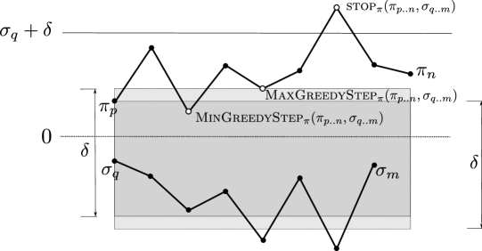
Figure 3: An illustration of greedy steps. For better visibility, the one-dimensional separated curves $\pi,\sigma$ are drawn in the plane by mapping $\pi_{i}$ to $(i,\pi_{i})$. In particular, the results of $\textsc{MinGreedyStep}_{\pi}(\pi_{p..n},\sigma_{q..m})$, $\textsc{MaxGreedyStep}_{\pi}(\pi_{p..n},\sigma_{q..m})$, and $\textsc{stop}_{\pi}(\pi_{p..n},\sigma_{q..m})$ are shown.

Theorem 4.6.

Let $\pi$ and $\sigma$ be separated curves in $\mathbb{R}$ and $\delta>0$. Algorithm 1 decides whether $d_{\mathrm{dF}}(\pi,\sigma)\leqslant\delta$ in time $\mathcal{O}((n+m)\log(nm))$.

We will first prove the correctness of the algorithm in Lemma 4.8 below and postpone the discussion how to implement the algorithm efficiently to Section 4.2.2.

4.2.1 Correctness

Note that Algorithm 1 considers potentially only very few points of the curve explicitly during its execution. Call the indices $(p,q)$ of point pairs considered in some iteration of the algorithm (for any choice of greedy steps, if more than one exists) greedy (point) pairs and all points contained in some such pair greedy points (of $\pi$ and $\sigma$). The following useful monotonicity property holds: If some greedy point on $\pi$ sees a point on $\sigma$ that is yet to be traversed, all following greedy points on $\pi$ will see it until it is traversed.

Lemma 4.7.

Let $(p_{1},q_{1}),\dots,(p_{i},q_{i})$ be the greedy point pairs considered in the iterations $1,\dots,i$. It holds that

1. $\mathrm{vis}_{\sigma}(\ell,q_{i})\subseteq\mathrm{vis}_{\sigma}(p_{i},q_{i})$ for all $1\leqslant\ell\leqslant p_{i}$, and

2. $\mathrm{vis}_{\pi}(p_{i},\ell)\subseteq\mathrm{vis}_{\pi}(p_{i},q_{i})$ for all $1\leqslant\ell\leqslant q_{i}$.

Proof.

Let $k<i$. We first show that $\mathrm{vis}_{\sigma}(\ell,q_{i})\subseteq\mathrm{vis}_{\sigma}(p_{k+1},q_{i})$ holds for all $p_{k}\leqslant\ell<p_{k+1}$. If $p_{k}=p_{k+1}$, the claim is immediate. Otherwise $p_{k+1}$ is the result of a greedy step on $\pi$. By definition of visibility, we have $\mathrm{vis}_{\sigma}(\ell,q_{i})=\mathrm{vis}_{\sigma}(\ell,q_{k})\cap[q_{i}..m]\subseteq\mathrm{vis}_{\sigma}(p_{k+1},q_{k})\cap[q_{i}..m]=\mathrm{vis}_{\sigma}(p_{k+1},q_{i})$, where the inequality follows from $p_{k+1}$ being a greedy step from $(p_{k},q_{k})$.

For arbitrary $\ell\leqslant i$, let $k<i$ be such that $p_{k}\leqslant\ell<p_{k+1}$. Then $\mathrm{vis}_{\sigma}(\ell,q_{i})\subseteq\mathrm{vis}_{\sigma}(p_{k+1},q_{i})\subseteq\mathrm{vis}_{\sigma}(p_{k+2},q_{i})\subseteq\cdots\subseteq\mathrm{vis}_{\sigma}(p_{i},q_{i})$. The second statement is symmetric. ∎

We will exploit this monotonicity to prove that if Algorithm 1 finds a greedy point pair that allows no further greedy steps, then no feasible traversal of $\pi$ and $\sigma$ exists. We derive an even stronger statement using the following notion: For a greedy point pair $(p,q)$, define $\textsc{stop}_{\pi}(\pi_{p..n},\sigma_{q..m}):=\operatorname{max}(\mathrm{reach}_{\pi}(p,q)\cup\{p\})+1$ as the index of the first point after $\pi_{p}$ on $\pi$ which is not seen by $\sigma_{q}$, or $n+1$ if no such index exists. Let $\textsc{stop}_{\sigma}$ be defined symmetrically.

Lemma 4.8 (Correctness of Algorithm 1).

Let $(p,q)$ be a greedy point of $\pi$ and $\sigma$, $p_{\mathrm{stop}}:=\textsc{stop}_{\pi}(\pi_{p..n},\sigma_{q..m})$ and $q_{\mathrm{stop}}:=\textsc{stop}_{\sigma}(\pi_{p..n},\sigma_{q..m})$. If on both curves, no greedy step from $(p,q)$ exists, then $d_{\mathrm{dF}}(\pi,\sigma)>\delta$.

In particular, if $q_{\mathrm{stop}}<m$, then for all $1\leqslant p^{\prime}\leqslant n$, we have that $d_{\mathrm{dF}}(\pi_{1..p^{\prime}},\sigma_{1..q_{\mathrm{stop}}})>\delta$ and if $p_{\mathrm{stop}}<n$, then $d_{\mathrm{dF}}(\pi_{1..p_{\mathrm{stop}}},\sigma_{1..q^{\prime}})>\delta$ for all $1\leqslant q^{\prime}\leqslant m$.

Note that the correctness of Algorithm 1 follows immediately: If the algorithm is stuck, then $d_{\mathrm{dF}}(\pi,\sigma)>\delta$. Otherwise, it finds a feasible traversal.

Proof of Lemma 4.8.

Consider the case that no greedy step from $(p,q)$ exists, then the following stuckness conditions have to hold:

1. For all $p^{\prime}\in\mathrm{reach}_{\pi}(p,q)$, we have $\mathrm{vis}_{\sigma}(p^{\prime},q)\subsetneq\mathrm{vis}_{\sigma}(p,q)$, and

2. for all $q^{\prime}\in\mathrm{reach}_{\sigma}(p,q)$, we have $\mathrm{vis}_{\pi}(p,q^{\prime})\subsetneq\mathrm{vis}_{\pi}(p,q)$.

In this case, we can extend the monotonicity property of Lemma 4.7 to include all reachable and the first unreachable point.

Claim 4.9.

If the stuckness conditions hold for $(p,q)$, then we have $\mathrm{vis}_{\sigma}(i,q)\subseteq\mathrm{vis}_{\sigma}(p,q)$ for all $1\leqslant i\leqslant p_{\mathrm{stop}}$. In particular, if $\pi_{p}$ does not see $\sigma_{\ell}$ for some $\ell>q$, then no vertex $\pi_{i}$ with $1\leqslant i\leqslant p_{\mathrm{stop}}$ sees $\sigma_{\ell}.$ The symmetric statement holds for $\sigma$.

Proof.

By the monotonicity of the previous claim, $\mathrm{vis}_{\sigma}(i,q)\subseteq\mathrm{vis}_{\sigma}(p,q)$ holds for all $i\leqslant p$. The first of the stuckness conditions implies $\mathrm{vis}_{\sigma}(i,q)\subseteq\mathrm{vis}_{\sigma}(p,q)$ for all $p<i<p_{\mathrm{stop}}$. If $p_{\mathrm{stop}}=n+1$, this already completes the proof of the claim. Otherwise, note that $\pi_{p_{\mathrm{stop}}}>\pi_{p}$, since otherwise $p_{\mathrm{stop}}\in\mathrm{reach}_{\pi}(p,q)$. Hence $\mathrm{vis}_{\sigma}(p_{\mathrm{stop}},q)\subseteq\mathrm{vis}_{\sigma}(p,q)$ holds as well. ∎

We distinguish the following cases that may occur under the stuckness conditions:

Case 1: $p_{\mathrm{stop}}\leqslant n$ or $q_{\mathrm{stop}}\leqslant m$. Without loss of generality, let $p_{\mathrm{stop}}\leqslant n$ (the other case is symmetric). Assume for contradiction that a feasible traversal $\phi$ of $\pi_{1..p_{\mathrm{stop}}}$ and $\sigma_{1..q^{\prime}}$ exists for some $1\leqslant q^{\prime}\leqslant m$. In $\phi$, at some point in time we have to move in $\pi$ from $p_{\mathrm{stop}}-1$ to $p_{\mathrm{stop}}$ while moving in $\sigma_{1..q^{\prime}}$ from some $\sigma_{\ell^{\prime}}$ to $\sigma_{\ell}$ where $\ell^{\prime}\in\{\ell-1,\ell\}$ and $\sigma_{\ell}$ sees $\pi_{p_{\mathrm{stop}}}$. Since $\sigma_{q}$ does not see $\pi_{p_{\mathrm{stop}}}$, the previous claim shows that $\ell>q_{\mathrm{stop}}$. If $q_{\mathrm{stop}}=m+1$ or $q_{\mathrm{stop}}<q^{\prime}$, this is impossible, yielding a contradiction. Otherwise, to do this transition, in some earlier step we have to move in $\sigma$ from $q_{\mathrm{stop}}-1$ to $q_{\mathrm{stop}}$ while moving in $\pi$ from $\pi_{k^{\prime}}$ to $\pi_{k}$ for some $k<p_{\mathrm{stop}}$ and $k^{\prime}\in\{k-1,k\}$. However, by definition $q_{\mathrm{stop}}\notin\mathrm{vis}_{\sigma}(p,q)$, hence Claim 4.9 implies that the transition is illegal, since $\pi_{k}$ does not see $\sigma_{q_{\mathrm{stop}}}$. This is a contradiction. By a symmetric argument, it holds that $d_{\mathrm{dF}}(\pi_{1..p^{\prime}},\sigma_{1..q_{\mathrm{stop}}})>\delta$.

Case 2: $p_{\mathrm{stop}}=n+1$ and $q_{\mathrm{stop}}=m+1$. In this case, $\mathrm{reach}_{\pi}(p,q)=[p+1..n]$ and $\mathrm{reach}_{\sigma}(p,q)=[q+1..n]$. By stuckness conditions, there exist an index $p_{\mathrm{max}}>p$ such that no $\sigma_{q^{\prime}}$ with $q^{\prime}>q$ sees $\pi_{p_{\mathrm{max}}}$ and an index $q_{\mathrm{min}}$ such that no $\pi_{p^{\prime}}$ with $p^{\prime}>p$ sees $\sigma_{q_{\mathrm{min}}}$. Assume for contradiction that a feasible traversal $\phi$ exists. In $\phi$, at some point in time $t$, we have to cross either (1) from $\pi_{p}$ to $\pi_{p+1}$ while moving in $\sigma$ from $\sigma_{\ell^{\prime}}$ to $\sigma_{\ell}$ with $\ell\leqslant q+1\leqslant q_{\mathrm{min}}$ and $\ell^{\prime}\in\{\ell-1,\ell\}$ or (2) from $\sigma_{q}$ to $\sigma_{q+1}$ while moving from $\pi_{\ell^{\prime}}$ to $\pi_{\ell}$ with $\ell\leqslant p+1\leqslant p_{\mathrm{max}}$ and $\ell^{\prime}\in\{\ell-1,\ell\}$. In the first case, $\ell<q_{\mathrm{min}}$ holds, since $\pi_{p+1}$ does not see $\sigma_{q_{\mathrm{min}}}$. For all consecutive times $t^{\prime}\geqslant t$, $\phi$ is in a point $\pi_{p^{\prime}}$ ($p^{\prime}\geqslant p+1$) that does not see $\sigma_{q_{\mathrm{min}}}$, which still has to be traversed, leading to a contradiction. Symmetrically, in the second case, for all times $t^{\prime}\geqslant t$, $\phi$ is in a point $\sigma_{q^{\prime}}$ $(q^{\prime}\geqslant q+1)$ that does not see $\pi_{p_{\mathrm{max}}}$, which still has to be traversed.

This concludes the proof of Lemma 4.8. ∎

4.2.2 Implementing greedy steps

To prove Theorem 4.6, it remains to show how to implement the algorithm to run in time $\mathcal{O}((n+m)\log(nm))$. We make use of geometric range search queries. The classic technique of fractional cascading [23, 13, 26] provides a data structure $D$ with the following properties: (i) Given $n$ points ${\cal P}$ in the plane, $D({\cal P})$ can be constructed in time $\mathcal{O}(n\log n)$ and (ii) given a query rectangle $Q:=I_{1}\times I_{2}$ with intervals $I_{1}$ and $I_{2}$, find and return $q\in Q\cap{\cal P}$ with minimal $y$-coordinate, or report that no such point exists, in time $\mathcal{O}(\log n)$. Here, each interval $I_{i}$ may be open, half-open or closed.

By invoking the above data structure on ${\cal P}:=\{(i,\pi_{i})\mid i\in[1\ldots n]\}$ for a given curve $\pi=\pi_{1..n}$ (as well as all three rotations of ${\cal P}$ by multiples of $90\degree$), we obtain a datastructure $\mathrm{D}^{\pi}$ such that:

1. $\mathrm{D}^{\pi}$ can be constructed in time $\mathcal{O}(n\log n)$,

2. the query $\mathrm{D}^{\pi}.\textsc{minIndex}([x_{1},x_{2}],[p,b])$ ($\mathrm{D}^{\pi}.\textsc{maxIndex}([x_{1},x_{2}],[p,b])$) returns the minimum (maximum) index $p\leqslant i\leqslant b$ such that $x_{1}\leqslant\pi_{i}\leqslant x_{2}$ in time $\mathcal{O}(\log n)$, and

3. the query $\mathrm{D}^{\pi}.\textsc{minHeight}([x_{1},x_{2}],[p,b])$ ($\mathrm{D}^{\pi}.\textsc{maxHeight}([x_{1},x_{2}],[p,b])$) returns the minimum (maximum) height $x_{1}\leqslant\pi_{i}\leqslant x_{2}$ such that $p\leqslant i\leqslant b$ in time $\mathcal{O}(\log n)$.

The queries extend naturally to open and half-open intervals. If no index exists in the queried range, all of these operations return the index $\infty$. We will use the corresponding data structure $\mathrm{D}^{\sigma}$ for $\sigma$ as well.

With these tools, we implement the following basic operations for arbitrary subcurves $\pi^{\prime}:=\pi_{p..b}$ and $\sigma^{\prime}:=\sigma_{q..d}$ of $\pi$ and $\sigma$. See also Figure 3.

1. Stopping points $\textsc{stop}_{\pi}(\pi^{\prime},\sigma^{\prime})$. For points $p,q$, $\textsc{stop}_{\pi}(\pi^{\prime},\sigma^{\prime}):=\operatorname{max}(\mathrm{reach}_{\pi^{\prime}}(p,q)\cup\{p\})+1$ returns the index of the first point after $\pi_{p}$ on $\pi^{\prime}$ which is not seen by $\sigma_{q}$, or $b+1$ if no such index exists.

   1:function $\textsc{stop}_{\pi}$($\pi_{p..b},\sigma_{q..d}$)

   2:     $p_{\mathrm{stop}}$ $\leftarrow$ $\mathrm{D}^{\pi}.\textsc{minIndex}((\sigma_{q}+\delta,\infty),[p,b]$) $\triangleright$ First non-visible point on $\pi$

   3:     if $p_{\mathrm{stop}}<\infty$ then return $p_{\mathrm{stop}}$

   4:     else return $b+1$      

   Algorithm 2 Finding the stopping point

2. Minimal greedy steps $\textsc{MinGreedyStep}_{\pi}(\pi^{\prime},\sigma^{\prime})$. This function returns the smallest index $p^{\prime}\in\mathrm{reach}_{\pi^{\prime}}(p,q)$ such that $\mathrm{vis}_{\sigma^{\prime}}(p^{\prime},q)\supseteq\mathrm{vis}_{\sigma^{\prime}}(p,q)$ or reports that no such index exists.

   1:function $\textsc{MinGreedyStep}_{\pi}$($\pi_{p..b},\sigma_{q..d}$)

   2:     $q_{\mathrm{min}}$ $\leftarrow$ $\mathrm{D}^{\sigma}.\textsc{minHeight}([\pi_{p}-\delta,\infty),[q,d])$ $\triangleright$ Lowest still visible point on $\sigma$

   3:     $p_{\mathrm{cand}}$ $\leftarrow$ $\mathrm{D}^{\pi}.\textsc{minIndex}((-\infty,\sigma_{q_{\mathrm{min}}}+\delta],[p+1,d]$) $\triangleright$ If $p^{\prime}$ exists, it is $p_{\mathrm{cand}}$

   4:     $p_{\mathrm{stop}}$ $\leftarrow$ $\textsc{stop}_{\pi}(\pi_{p..b},\sigma_{q..d})$ $\triangleright$ First non-visible point on $\pi$

   5:     if $p_{\mathrm{cand}}<p_{\mathrm{stop}}$ then return $p_{\mathrm{cand}}$

   6:     else return “No greedy step possible.” $\triangleright$ $\pi_{p_{\mathrm{cand}}}$ not reachable from $\pi_{p}$ while staying in $\sigma_{q}$      

   Algorithm 3 Minimal greedy step

3. Maximal greedy steps $\textsc{MaxGreedyStep}_{\pi}(\pi^{\prime},\sigma^{\prime})$. Let $p^{\prime}\in\mathrm{reach}_{\pi^{\prime}}(p,q)$ be such that (i) $p^{\prime}$ is the largest index maximizing $|\mathrm{vis}_{\sigma^{\prime}}(z,q)|$ among all $z\in\mathrm{reach}_{\pi^{\prime}}(p,q)$ and (ii) $\mathrm{vis}_{\sigma^{\prime}}(p^{\prime},q)\supseteq\mathrm{vis}_{\sigma^{\prime}}(p,q)$. If $p^{\prime}$ exists, $\textsc{MaxGreedyStep}_{\pi}$ returns this value, otherwise it reports that no such index exists. Note that if $p^{\prime}$ exists, then by definition there is no greedy step on $\pi$ starting from $(p^{\prime},q)$, i.e., this step is a maximal greedy step.

   1:function $\textsc{MaxGreedyStep}_{\pi}$($\pi_{p..b},\sigma_{q..d}$)

   2:     $q_{\mathrm{min}}$ $\leftarrow$ $\mathrm{D}^{\sigma}.\textsc{minHeight}([\pi_{p}-\delta,\infty),[q,d])$ $\triangleright$ Lowest still visible point on $\sigma$

   3:     $p_{\mathrm{stop}}$ $\leftarrow$ $\textsc{stop}_{\pi}(\pi_{p..b},\sigma_{q..d})$ $\triangleright$ First non-visible point on $\pi$

   4:     $p_{\mathrm{min}}$ $\leftarrow$ $\mathrm{D}^{\pi}.\textsc{minHeight}((-\infty,\sigma_{q_{\mathrm{min}}}+\delta],[p+1,p_{\mathrm{stop}}-1]$) $\triangleright$ Maximizes visibility among reachable points

   5:     if $p_{\mathrm{min}}=\infty$ then

   6:         return “No greedy step possible.” $\triangleright$ No reachable point has better visibility than $\pi_{p}$

   7:     else

   8:         $q_{\mathrm{min}}$ $\leftarrow$ $\mathrm{D}^{\sigma}.\textsc{minHeight}([\pi_{p_{\mathrm{min}}}-\delta,\infty),[q,d])$ $\triangleright$ Lowest point on $\sigma$ still seen by $p_{\mathrm{min}}$

   9:         return $\mathrm{D}^{\pi}.\textsc{maxIndex}((-\infty,\sigma_{q_{\mathrm{min}}}+\delta],[p_{\mathrm{min}},p_{\mathrm{stop}}-1])$      

   Algorithm 4 Maximal greedy step

4. Arbitrary greedy steps $\textsc{GreedyStep}_{\pi}(\pi^{\prime},\sigma^{\prime})$. If, in some situation, it is only required to find an arbitrary index $p^{\prime}\in\mathrm{reach}_{\pi^{\prime}}(p,q)$ such that all $p\leqslant i\leqslant p^{\prime}$ satisfy $\mathrm{vis}_{\sigma^{\prime}}(i,q)\subseteq\mathrm{vis}_{\sigma^{\prime}}(p^{\prime},q)$ or report that no such index exists, we use the function $\textsc{GreedyStep}_{\pi}(\pi^{\prime},\sigma^{\prime})$ to denote that any such function suffices; in particular, $\textsc{MinGreedyStep}_{\pi}$ or $\textsc{MaxGreedyStep}_{\pi}$ can be used.

For $\sigma$, we define the obvious symmetric operations. Note that in these operations, it is not feasible to traverse all directly feasible points and check whether the visibility criterion is satisfied, since this would not necessarily yield a running time of $\mathcal{O}^{*}(1)$.

Lemma 4.10.

Using $O((n+m)\log nm)$ preprocessing time, $\textsc{MaxGreedyStep}_{\pi}$, $\textsc{MinGreedyStep}_{\pi}$ and $\textsc{stop}_{\pi}$ can be implemented to run in time $\mathcal{O}(\log nm)$.

Proof.

In time $\mathcal{O}((n+m)\log nm)$, we can build the data structure $\mathrm{D}^{\pi}$ for $\pi$ and symmetrically $\mathrm{D}^{\sigma}$ for $\sigma$. Algorithms 2, 3 and 4 implement the greedy steps and $\textsc{stop}_{\pi}$ using only a constant number of queries to $\mathrm{D}^{\pi}$ and $\mathrm{D}^{\sigma}$, each with running time $\mathcal{O}(\log n)$ or $\mathcal{O}(\log m)$. ∎

For the reduced free-space problem, these operations can be implemented even faster.

Lemma 4.11.

Let $\pi=\pi_{1..n}$ and $\sigma=\sigma_{1..m}$ be input curves of the reduced free-space problem. Using $O((n+m)\log 1/\varepsilon)$ preprocessing time, $\textsc{MaxGreedyStep}_{\pi}$, $\textsc{MinGreedyStep}_{\pi}$ and $\textsc{stop}_{\pi}$ can be implemented to run in time $\mathcal{O}(\log 1/\varepsilon)$.

Proof.

We argue that range searching can be implemented with $\mathcal{O}(\log 1/\varepsilon)$ query time and $\mathcal{O}(n\log 1/\varepsilon)$ preprocessing time. This holds since for the point set ${\cal P}=\{(i,\pi_{i})\mid i\in[1\ldots n]\}$ (1) the $x$-values are $1,\ldots,n$, so that we can determine the relevant pointers in the first level of the fractional-cascading tree in constant time instead of $\mathcal{O}(\log n)$ and (2) all $y$-values are multiples of $\tfrac{1}{3}\varepsilon\delta$ and in $[-2\delta,2\delta]$, i.e., there are only $\mathcal{O}(1/\varepsilon)$ different $y$-values. For the latter, note that any point $\pi_{p}>\delta$ sees no point in $\sigma$, and this is preserved by setting $\pi_{p}$ to $2\delta$ (and similarly for $\sigma$). Using these properties it is straightforward to adapt the fractional-cascading data structure, we omit the details. ∎

4.3 Composition of one-dimensional curves

In this subsection, we collect essential composition properties of feasible traversals of one-dimensional curves that enable us to tackle the reduced free-space problem (see Figure 4 for an illustration of these results). The first tool is a union lemma that states that two intersecting intervals $I,J$ of $\pi$ that each have a feasible traversal together with $\sigma$ prove that also $\pi_{I\cup J}$ can be traversed together with $\sigma$.

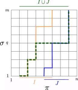
(a) Lemma 4.12

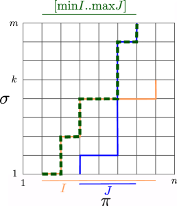
(b) Lemma 4.13

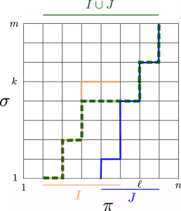
(c) Lemma 4.14

Figure 4: Composition properties of feasible traversals of one-dimensional separated curves.

Lemma 4.12.

Let $\pi=\pi_{1..n}$ and $\sigma=\sigma_{1..m}$ be one-dimensional separated curves and let $I,J\subseteq[1..n]$ be intervals with $I\cap J\neq\emptyset$. If $d_{\mathrm{dF}}(\pi_{I},\sigma)\leqslant\delta$ and $d_{\mathrm{dF}}(\pi_{J},\sigma)\leqslant\delta$, then $d_{\mathrm{dF}}(\pi_{I\cup J},\sigma)\leqslant\delta$.

Proof.

If $I\subseteq J$, the claim is trivial. W.l.o.g, let $I=[a_{I}..b_{I}]$ and $J=[a_{J}..b_{J}]$, where $a_{I}\leqslant a_{J}\leqslant b_{I}\leqslant b_{J}$. Let $\phi_{I}$ (and $\phi_{J}$) be a feasible traversal of $(\pi_{I},\sigma)$ (and $(\pi_{J},\sigma)$, respectively). By reparameterization, we can assume that $\phi_{I}(t)=(\psi_{I}(t),f(t))$ and $\phi_{J}(t)=(\psi_{J}(t),f(t))$ for suitable (non-decreasing onto) functions $\psi_{I},\psi_{J}:[0,1]\to[1..n]$ and $f:[0,1]\to[1..m]$. One of the following cases occurs.

Case 1: There is some $0\leqslant t\leqslant 1$ with $\psi_{I}(t)=\phi_{J}(t)$. Then we can concatenate $\phi_{I}(0,t)$ and $\phi_{J}(t,1)$ to obtain a feasible traversal of $\phi_{I\cup J}$.

Case 2: For all $0\leqslant t\leqslant 1$, we have $\psi_{I}(t)<\psi_{J}(t)$. Let $\sigma_{q}$ be the highest point on $\sigma$. By $d_{\mathrm{dF}}(\pi_{I},\sigma)\leqslant\delta$ and $d_{\mathrm{dF}}(\pi_{J},\sigma)\leqslant\delta$, the point $\sigma_{q}$ sees all points on $\pi_{I\cup J}$. There is some $0\leqslant t^{\ast}\leqslant 1$ with $f(t^{\ast})=q$. We can concatenate $\phi_{I}(0,t)$ and the traversal of $\pi_{\psi_{I}(t^{\ast})..\psi_{J}(t^{\ast})}$ and $\sigma_{q}$ to obtain a feasible traversal of $\pi_{a_{I}..\psi_{I}(t^{\ast})}$ and $\sigma_{1..f(t^{\ast})}$. Appending $\phi_{J}(t^{\ast},1)$ to this traversal yields $d_{\mathrm{dF}}(\pi_{a_{I}..b_{J}},\sigma)\leqslant\delta$. ∎

The second result formalizes situations in which a traversal $\phi$ of subcurves has to cross a traversal $\psi$ of other subcurves, yielding the possibility to follow $\phi$ up to the crossing point and to follow $\psi$ from there on.

Lemma 4.13.

Let $\pi=\pi_{1..n}$ and $\sigma=\sigma_{1..m}$ be one-dimensional curves and consider intervals $I=[a_{I}..b_{I}]$ and $J=[a_{J}..b_{J}]$ with $J\subseteq I\subseteq[1..n]$, and $K=[1..k]\subseteq[1..m]$. If $d_{\mathrm{dF}}(\pi_{I},\sigma_{K})\leqslant\delta$ and $d_{\mathrm{dF}}(\pi_{J},\sigma)\leqslant\delta$, then $d_{\mathrm{dF}}(\pi_{a_{I}..b_{J}},\sigma)\leqslant\delta$.

Proof.

Let $\phi$ be a feasible traversal of $\pi_{I}$ and $\sigma_{K}$ and $\psi$ a feasible traversal of $\pi_{J}$ and $\sigma$. We first show that $\phi$ and $\psi$ cross, i.e., there are $0\leqslant t,t^{\prime}\leqslant 1$ such that $\phi(t)=\psi(t^{\prime})$. For all $k\in[1..K]$, let $[s_{k}^{\phi}..e_{k}^{\phi}]$ denote the interval of points that $\phi$ traverses on $\pi$ while staying in $\sigma_{k}$. Similarly, $[s_{k}^{\psi}..e_{k}^{\psi}]$ denotes the interval of points $\psi$ traverses on $\pi$ while staying in $\sigma_{k}$. Assume for contradiction that $[s_{k}^{\phi}..e_{k}^{\phi}]$ and $[s_{k}^{\psi}..e_{k}^{\psi}]$ are disjoint for all $1\leqslant k\leqslant K$. Then initially, we have $s_{1}^{\phi}=a_{I}\leqslant a_{J}=s_{1}^{\psi}$ and hence $e_{1}^{\phi}<s_{1}^{\psi}$. This implies $s_{2}^{\phi}\leqslant e_{1}^{\phi}+1\leqslant s_{1}^{\psi}\leqslant s_{2}^{\psi}$ and inductively we obtain $e_{k}^{\phi}<s_{k}^{\psi}\leqslant e_{k}^{\psi}$ for all $k\in[1..K]$. This contradicts $e_{K}^{\phi}=b_{I}\geqslant b_{J}\geqslant e_{K}^{\psi}$. Hence, for some $1\leqslant k\leqslant K$, $[s_{k}^{\phi}..e_{k}^{\phi}]$ and $[s_{k}^{\psi}..e_{k}^{\psi}]$ intersect, which gives $\phi(t)=(p,k)=\psi(t^{\prime})$ for any $p\in[s_{k}^{\phi},e_{k}^{\phi}]\cap[s_{k}^{\psi},e_{k}^{\psi}]$ and the corresponding $0\leqslant t,t^{\prime}\leqslant 1$. By concatenating $\phi(0,t)$ with $\psi(t^{\prime},1)$, we obtain a feasible traversal of $\pi_{a_{I}..b_{J}}$ and $\sigma$.∎

The last result in our composition toolbox strengthens Lemma 4.12 to the case that the traversal of $\pi_{I}$ uses only an initial subcurve $\sigma_{1..k}$ of $\sigma$ and not the complete curve.

Lemma 4.14.

Let $\pi=\pi_{1..n}$ and $\sigma=\sigma_{1..m}$ be one-dimensional separated curves and consider intervals $I=[a_{I}..b_{I}]$ and $J=[a_{J}..b_{J}]$ with $1\leqslant a_{I}\leqslant a_{J}\leqslant b_{I}\leqslant b_{J}\leqslant n$, and $K=[1..k]\subseteq[1..m]$. If $d_{\mathrm{dF}}(\pi_{I},\sigma_{K})\leqslant\delta$ and $d_{\mathrm{dF}}(\pi_{J},\sigma)\leqslant\delta$, then $d_{F}(\pi_{I\cup J},\sigma)\leqslant\delta$.

Proof.

Let $\phi$ be any feasible traversal of $\pi_{J}$ and $\sigma$. There exists $a_{J}\leqslant\ell\leqslant b_{J}$ with $\phi(t)=(\ell,k)$ for some $0\leqslant t\leqslant 1$. Hence $\phi$ restricted to $[0,t]$ yields a feasible traversal of $\pi_{a_{J}..\ell}$ and $\sigma_{K}$, i.e., $d_{\mathrm{dF}}(\pi_{a_{J}..\ell},\sigma_{K})\leqslant\delta$. Since $I$ and $[a_{J}..\ell]$ are intersecting, Lemma 4.12 yields that $d_{\mathrm{dF}}(\pi_{a_{I}..\ell},\sigma_{K})\leqslant\delta$. Let $\psi$ be such a feasible traversal of $\pi_{a_{I}..\ell}$ and $\sigma_{K}$. Concatenating $\psi$ at $\psi(1)=(\ell,k)=\phi(t)$ with $\phi(t,1)$, we construct a feasible traversal of $\pi_{a_{I}..b_{J}}$ and $\sigma$, proving the claim. ∎

4.4 Solving the Reduced Free-space Problem

In this section, we solve the reduced free-space problems, using the structural properties derived in the previous section and the principles underlying the greedy algorithm of Section 4.2. Recall that the greedy steps implemented as discussed in Section 4.2.2 run in time $\mathcal{O}(\log 1/\varepsilon)$ on the input curves of the reduced free-space problem.

4.4.1 Single Entry

Given the separated curves $\pi=(\pi_{1},\dots,\pi_{n})$ and $\sigma=(\sigma_{1},\dots,\sigma_{m})$ and entry set $E=\{1\}$, we show how to compute $F^{\sigma}$. We present the following recursive algorithm.

1:

2:function Find-$\sigma$-exits($\pi_{p..b},\sigma_{q..d}$)

3:     if $q=d$ then

4:         if $\textsc{stop}_{\pi}(\pi_{p..b},\sigma_{q})=b+1$ then

5:              return $\{q\}$ $\triangleright$ The end of $\pi$ is reachable while staying in $\sigma_{q}$

6:         else return $\emptyset$               

7:

8:     if $p^{\prime}\leftarrow\textsc{MaxGreedyStep}_{\pi}(\pi_{p..b},\sigma_{q..d})$ then

9:         return Find-$\sigma$-exits($\pi_{p^{\prime}..b},\sigma_{q..d})$)

10:     else if $q^{\prime}\leftarrow\textsc{GreedyStep}_{\sigma}(\pi_{p..b},\sigma_{q..d})$ then

11:         return $\textsc{Find-$\sigma$-exits}(\pi_{p..b},\sigma_{q..q^{\prime}-1})\cup\textsc{Find-$\sigma$-exits}(\pi_{p..b},\sigma_{q^{\prime}..d})$

12:     else

13:         return $\textsc{Find-$\sigma$-exits}(\pi_{p..b},\sigma_{q..d-1})$ $\triangleright$ No greedy step possible      

Algorithm 5 Special Case: Single entry

The following property establishes that a greedy step on a long curve is also a greedy step on a shorter curve. Clearly, the converse does not necessarily hold.

Proposition 4.15.

Let $1\leqslant p\leqslant P\leqslant n$ and $1\leqslant q\leqslant Q\leqslant m$. Any greedy step on $\pi$ from $(p,q)$ to $(p^{\prime},q)$ with $p^{\prime}\leqslant P$ is also a greedy step with respect to $\tilde{\pi}:=\pi_{p..P}$ and $\tilde{\sigma}:=\sigma_{q..Q}$, i.e., if there is some $p^{\prime}\leqslant P$ with $\mathrm{vis}_{\sigma}(i,q)\subseteq\mathrm{vis}_{\sigma}(p^{\prime},q)$ for all $p\leqslant i\leqslant p^{\prime}$, then also $\mathrm{vis}_{\tilde{\sigma}}(i,q)\subseteq\mathrm{vis}_{\tilde{\sigma}}(p^{\prime},q)$.

Proof.

From the definition of $\mathrm{vis}_{\sigma}$, we immediately derive $\mathrm{vis}_{\tilde{\sigma}}(i,q)=\mathrm{vis}_{\sigma}(i,q)\cap[q..Q]\subseteq\mathrm{vis}_{\sigma}(p^{\prime},q)\cap[q..Q]=\mathrm{vis}_{\tilde{\sigma}}(p^{\prime},q)$ for all $p\leqslant i\leqslant p^{\prime}$. Restricting the length of $\pi$ also has no influence on the greedy property, except for the trivial requirement that $p^{\prime}$ still has to be contained in the restricted curve.∎

Lemma 4.16.

Algorithm 5 correctly identifies $F^{\sigma}$ given the single entry $E=\{1\}$.

Proof.

Clearly, if $\textsc{Find-$\sigma$-exits}(\pi,\sigma)$ finds and returns an exit $e$ on $\sigma$, then it is contained in $F^{\sigma}$, since the algorithm uses only feasible (greedy) steps. Conversely, we show that for all $I=[p..b]$ and $J=[q..d]$, where $(p,q)$ is a greedy point pair of $\pi$ and $\sigma$, and all $e\in J$ with $d_{\mathrm{dF}}(\pi_{I},\sigma_{J\cap[1..e]})\leqslant\delta$, we have $e\in\textsc{Find-$\sigma$-Exits}(\pi_{I},\sigma_{J})$, i.e. we find all exits.

Consider some call of $\textsc{Find-$\sigma$-Exits}(\pi_{I},\sigma_{J})$ for which the precondition is fulfilled. If $J$ consists only of a single point, then $J=\{e\}$, and a feasible traversal of $\pi_{I}$ and $\sigma_{J}$ exists if and only if $\sigma_{e}$ sees all points on $\pi_{I}$. Let $I=[p..b],$ then this happens if and only if $\textsc{stop}_{\pi}(\pi_{I},\sigma_{e})=b+1$, hence the base case is treated correctly.

Assume that $I=[p..b]$ and a maximal greedy step $p^{\prime}$ on $\pi$ exists. By Property 4.15, this step is a greedy step also with respect to $\sigma_{J\cap[1..e]}$. Hence by Lemma 4.8, if there is a traversal of $\pi_{p..b}$ and $\sigma_{J\cap[1..e]}$, then a traversal of $\pi_{[p^{\prime}..b]}$ and $\sigma_{J\cap[1..e]}$ also exists.

Consider the case in which $J=[q..d]$ and a greedy step $q^{\prime}$ in $\sigma$ exists. If $e<q^{\prime}$, then $e\in[q..q^{\prime}-1]$ and $J\cap[1..e]=[q..q^{\prime}-1]\cap[1..e]$. Hence, $e$ is found in the recursive call with $J^{\prime}=[q..q^{\prime}-1]$. If $e\geqslant q^{\prime}$, then by Property 4.15, this step is a greedy step with respect to the curves $\pi_{I}$ and $\sigma_{J\cap[1..e]}$. Again, by Lemma 4.8, the existence of a feasible traversal of $\pi_{I}$ and $\sigma_{J}$ implies that also a feasible traversal of $\pi_{I}$ and $\sigma_{J\cap[q^{\prime}..e]}$ exists.

It remains to regard the case in which no greedy step exists. By Lemma 4.8, there is no feasible traversal of $\pi_{1..n}$ and $\sigma_{1..d}$. This implies $e\neq d$ and all exits are found in the recursive call with $J^{\prime}=[q,d-1]$.∎

Lemma 4.17.

$\textsc{Find-$\sigma$-Exits}(\pi_{p..b},\sigma_{q..d})$ runs in time $\mathcal{O}((d-q+1)\cdot\log 1/\varepsilon)$.

Proof.

Since the algorithm’s greedy steps on $\pi$ are maximal, after each greedy step on $\pi$, we split $\sigma$ (by a greedy step on $\sigma$) or shorten $\sigma$ (if no greedy step on $\sigma$ is found). Thus, it takes at most $\mathcal{O}(\log 1/\varepsilon)$ time until $\sigma$ is split or shortened. The base case is also handled in time $\mathcal{O}(\log 1/\varepsilon)$. In total, this yields a running time of $\mathcal{O}((d-q+1)\log 1/\varepsilon)$. ∎

Note that by swapping the roles of $\pi$ and $\sigma$, Find-$\sigma$-Exits can be used to determine $F^{\pi}$ given the single entry $\sigma_{1}$ on $\sigma$. This is equivalent to having the single entry $E=\{1\}$ on $\pi$. Thus, we can also implement the function $\textsc{Find-$\pi$-Exits}(\pi_{1..n},\sigma_{1..m})$ that returns $F^{\pi}$ given the single entry $E=\{1\}$ in time $\mathcal{O}(n\log 1/\varepsilon)$.

4.4.2 Entries on $\pi$, Exits on $\pi$

In this section, we tackle the task of determining $F^{\pi}$ given a set of entries $E$ on $\pi$. It is essential to avoid computing the exits by iterating over every single entry. We show how to divide $\pi$ into disjoint subcurves that can be solved by a single call to Find-$\pi$-Exits each.

Assume we want to traverse $\pi_{p..b}$ and $\sigma_{q..d}$ starting in $\pi_{p}$ and $\sigma_{q}$. Let $u(p):=\operatorname{max}\{p^{\prime}\in[p,b]\mid\exists q\leqslant q^{\prime}\leqslant d:d_{\mathrm{dF}}(\pi_{p..p^{\prime}},\sigma_{q..q^{\prime}})\leqslant\delta\}$ be the last point on $\pi$ that is reachable while traversing an arbitrary subcurve of $\sigma_{q..d}$ that starts in $\sigma_{q}$. This point fulfills the following properties.

Lemma 4.18.

It holds that

1. If there are $p\leqslant e\leqslant e^{\prime}\leqslant u(p)$ with $d_{\mathrm{dF}}(\pi_{e..e^{\prime}},\sigma_{q..d})\leqslant\delta$, then $d_{\mathrm{dF}}(\pi_{p..e^{\prime}},\sigma_{q..d})\leqslant\delta$.

2. For all $p\leqslant e\leqslant u(p)<e^{\prime}$, we have that $d_{\mathrm{dF}}(\pi_{e..e^{\prime}},\sigma_{q..d})>\delta$.

Proof.

By definition of $u(p)$, there is a $q\leqslant q^{\prime}\leqslant d$ with $d_{\mathrm{dF}}(\pi_{p..u(p)},\sigma_{q..q^{\prime}})\leqslant\delta$. Since $[e,e^{\prime}]\subseteq[p,u(p)]$, Lemma 4.13 proves the first statement. For the second statement, assume for contradiction that $d_{\mathrm{dF}}(\pi_{e..e^{\prime}},\sigma_{q..d})\leqslant\delta$. Then, Lemma 4.14 yields that $d_{\mathrm{dF}}(\pi_{p..e^{\prime}},\sigma_{q..d})\leqslant\delta$. This is a contradiction to the choice of $u(p)$, since $e^{\prime}>u(p)$. ∎

The above lemma implies that we can ignore all entries in $[p..u(p)]$ except for $p$ and that all exits reachable from $p$ are contained in the interval $[p..u(p)]$. This gives rise to the following algorithm.

1:

2:function $\pi$-exits-from-$\pi$($\pi,\sigma,E$)

3:     $S\leftarrow\emptyset$

4:     while $E\neq\emptyset$ do

5:         $\hat{p}$ $\leftarrow$ pop minimal index from $E$

6:         $p\leftarrow\hat{p}$, $q\leftarrow 1$

7:         repeat

8:              if $q^{\prime}\leftarrow\textsc{MaxGreedyStep}_{\sigma}(\pi_{p..n},\sigma_{q..m})$ then

9:                  $q$ $\leftarrow$ $q^{\prime}$               

10:              if $p^{\prime}\leftarrow\textsc{GreedyStep}_{\pi}(\pi_{p..n},\sigma_{q..m})$ then

11:                  $p$ $\leftarrow$ $p^{\prime}$               

12:         until no greedy step was found in the last iteration

13:         $\overline{p}$ $\leftarrow$ $\textsc{stop}_{\pi}(\pi_{p..n},\sigma_{q..m})-1$ $\triangleright$ determines the maximal reachable point $u(\hat{p})$

14:         $S$ $\leftarrow$ $S\cup\textsc{Find-$\pi$-Exits}(\pi_{\hat{p}..\overline{p}},\sigma)$

15:         $E$ $\leftarrow$ $E\cap[\overline{p}+1,n]$ $\triangleright$ drops all entries in $[\hat{p},u(\hat{p})]$      

16:     return $S$

Algorithm 6 Given entry points $E$ on $\pi$, compute all exits on $\pi$.

Lemma 4.19.

Algorithm 6 correctly computes $F^{\pi}$.

Proof.

We first argue that for each considered entry $\hat{p}$, the algorithm computes $\overline{p}=u(\hat{p})$. Clearly, $\overline{p}\leqslant u(\hat{p})$, since only feasible steps are used to reach $\overline{p}$. If $\overline{p}=m$, this already implies that also $u(\hat{p})=m$. Otherwise, let $(p,q)$ be the greedy point pair on the curves $\pi_{\hat{p}\ldots n}$ and $\sigma$ for which no greedy step has been found. Then by Lemma 4.8, for $p_{\mathrm{stop}}:=\textsc{stop}_{\pi}(\pi_{p..n},\sigma_{q..m})$ and all $1\leqslant q^{\prime}\leqslant m$, we have that $d_{\mathrm{dF}}(\pi_{\hat{p}..p_{\mathrm{stop}}},\sigma_{1..q^{\prime}})>\delta$. Hence, $u(\hat{p})<p_{\mathrm{stop}}$. Finally, note that Algorithm 6 computes $\overline{p}=p_{\mathrm{stop}}-1$, which proves $\overline{p}=u(\hat{p})$.

It is clear that every found exit is included in $F^{\pi}$. Conversely, let $e^{\prime}\in F^{\pi}$ and $1\leqslant e\leqslant n$ be such that $d_{\mathrm{dF}}(\pi_{e..e^{\prime}},\sigma)\leqslant\delta$. For some $\hat{p}$ with $\hat{p}\leqslant e\leqslant u(\hat{p})=\overline{p}$, we run $\textsc{Find-$\pi$-Exits}(\pi_{\hat{p}..\overline{p}},\sigma)$. Hence by Lemma 4.18 (2), $e^{\prime}\leqslant u(\hat{p})$ and by Lemma 4.18 (1), $d_{\mathrm{dF}}(\pi_{\hat{p}..e^{\prime}},\sigma)\leqslant\delta$. Hence, the corresponding call $\textsc{Find-$\pi$-Exits}(\pi_{\hat{p}..\overline{p}},\sigma)$ will find $e^{\prime}$.∎

Lemma 4.20.

Using preprocessing time $\mathcal{O}((n+m)\log 1/\varepsilon)$, Algorithm 6 runs in time $\mathcal{O}(n\log 1/\varepsilon)$.

Proof.

We first bound the cost of all calls $\textsc{Find-$\pi$-Exits}(\pi_{I_{i}},\sigma)$. Clearly, all intervals $I_{i}$ are disjoint with $\bigcup I_{i}\subseteq[1..n]$. Hence, by Lemma 4.17, the total time spent in these calls is bounded by $\mathcal{O}(\sum_{i}|I_{i}|\log(1/\varepsilon))=\mathcal{O}(n\log 1/\varepsilon)$. To bound the number greedy steps, let $p_{1},\dots,p_{k}$ be the distinct indices considered as values of $p$ during the execution of $\mbox{{$\pi$-exits-from-$\pi$}}(\pi,\sigma)$. Between changing $p$ from each $p_{i}$ to $p_{i+1}$, we will make, by maximality, at most one call to $\textsc{MaxGreedyStep}_{\sigma}$ and at most call to $\textsc{GreedyStep}_{\pi}$. Since $k\leqslant n,$ the total cost of greedy calls is bounded by $\mathcal{O}(n\log 1/\varepsilon)$ as well. The total time spent in all other operations is bounded by $\mathcal{O}(n\log 1/\varepsilon)$. ∎

4.4.3 Entries on $\pi$, Exits on $\sigma$

Similar to the previous section, we show how to compute the exits $F^{\sigma}$ given entries $E$ on $\pi$, by reducing the problem to calls of Find-$\sigma$-Exits on subcurves of $\pi$ and $\sigma$. This time, however, the task is more intricate. For any index $p$ on $\pi$, let $Q(p):=\operatorname{min}\{q\mid d_{\mathrm{dF}}(\pi_{p..n},\sigma_{1..q})\leqslant\delta\}$ be the endpoint of the shortest initial fragment of $\sigma$ such that the remaining part of $\pi$ can be traversed together with this fragment. Let $P(p):=\operatorname{min}\{p^{\prime}\mid d_{\mathrm{dF}}(\pi_{p..p^{\prime}},\sigma_{1..Q(p)})\leqslant\delta\}$ be the endpoint of the shortest initial fragment of $\pi$, such that $\sigma_{Q(p)}$ can be reached by a feasible traversal.

Note that by definition, entries $p$ with $Q(p)=\infty$ are irrelevant for determining the exits on $\sigma$. In fact, if an entry $p$ is relevant, i.e., $Q(p)<\infty$, it is easy to compute $Q(p)$ due to the following lemma.

Lemma 4.21.

Let $Q^{\prime}(p):=\operatorname{min}\{q\mid\sigma_{q}\geqslant\operatorname{max}_{i\in[p..n]}\pi_{i}-\delta\}$. If $Q(p)<\infty$, then $Q(p)=Q^{\prime}(p)$. Similarly, $Q(p)<\infty$ implies that $P(p)=\operatorname{min}\{p^{\prime}\mid\pi_{p^{\prime}}\leqslant\operatorname{min}_{i\in[q..Q(p)]}\sigma_{i}+\delta\}<\infty$.

Proof.

Assume that $Q(p)<Q^{\prime}(p)$ holds, then no point in $\sigma_{1..Q(p)}$ sees the highest point in $\pi_{p..n}$. Hence no feasible traversal of these curves can exist, yielding a contradiction. Assume that $Q(p)>Q^{\prime}(p)$ holds instead and consider the feasible traversal $\phi$ of the shortest initial fragment of $\sigma$ that passes through all points in $\pi_{p..n}$. At some point $\phi$ visits $(\pi_{p^{\prime}},\sigma_{Q^{\prime}(p)})$ for some $p\leqslant p^{\prime}\leqslant n$. We can alter this traversal to pass through the remaining curve $\pi_{p^{\prime}..n}$ while staying in $\sigma_{Q^{\prime}(p)}$, since $\sigma_{Q^{\prime}(p)}$ sees all points on $\pi_{p^{\prime}..n}$. This gives a feasible traversal of $\pi_{p..n}$ and $\sigma_{1..Q^{\prime}(p)}$, which is a contradiction to the choice of $\phi$ and $Q(p)>Q^{\prime}(p)$.

The statement for $P(p)$ follows analogously by regarding the curves $\pi_{p..n}$ and $\sigma_{1..Q(p)}$ and switching their roles. ∎

Note that the previous lemma shows that for relevant entries $p_{1}<p_{2}$, we have $Q(p_{1})\geqslant Q(p_{2})$, since for relevant entries, $Q(p_{1})=Q^{\prime}(p_{1})\geqslant Q^{\prime}(p_{2})=Q(p_{2})$. We will use the following lemma to argue that (i) if $Q(p_{1})=Q(p_{2})$, entry $p_{1}$ dominates $p_{2}$, and (2) if $Q(p_{1})>Q(p_{2})$, we have $p_{2}\notin[p_{1}..P(p_{1})]$. Hence, we can ignore all entries in $[p_{1}..P(p_{1})]$ except for $p_{1}$ itself.

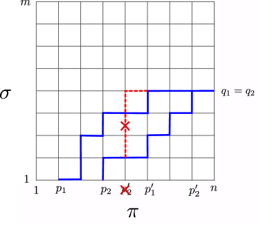
(a) Case $q_{1}=q_{2}$.

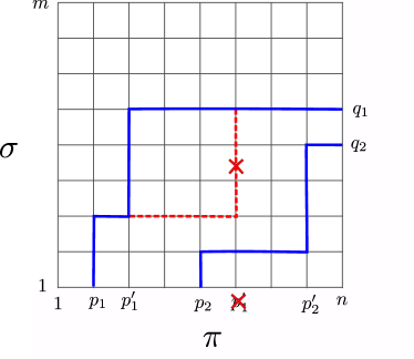
(b) Case $q_{1}>q_{2}$.

Figure 5: Illustration of Lemma 4.22. For both $p_{i}$, $i\in\{1,2\}$, a feasible traversal of the curves $\pi_{p_{i}..p_{i}^{\prime}}$ and $\sigma_{1..q_{i}}$ is depicted as monotone paths in the free-space.

Lemma 4.22.

Let $p_{1}<p_{2}$ be indices on $\pi$ with $q_{1}:=Q(p_{1})<\infty$ and $q_{2}:=Q(p_{2})<\infty$. Let $p^{\prime}_{1}:=P(p_{1})$ and $p^{\prime}_{2}:=P(p_{2})$. If $q_{1}=q_{2}$, then $p_{1}^{\prime}\leqslant p_{2}^{\prime}$. Otherwise, i.e., if $q_{1}>q_{2}$, we even have $p^{\prime}_{1}<p_{2}$.

Proof.

See Figure 5 for illustrations. Let $q_{1}=q_{2}$. Assume for contradiction that $p^{\prime}_{1}>p_{2}^{\prime}$, then we have $d_{\mathrm{dF}}(\pi_{p_{1}..p_{1}^{\prime}},\sigma_{1..q_{1}})\leqslant\delta$ and $d_{\mathrm{dF}}(\pi_{p_{2}..p_{2}^{\prime}},\sigma_{1..q_{1}})\leqslant\delta$, where $[p_{2}..p_{2}^{\prime}]\subseteq[p_{1}..p_{1}^{\prime}]$. Hence by Lemma 4.13, $d_{\mathrm{dF}}(\pi_{p_{1}..p_{2}^{\prime}},\sigma_{1..q_{1}})\leqslant\delta$ and thus $p_{1}^{\prime}\leqslant p_{2}^{\prime}$, which is a contradiction to the assumption.

For the second statement, let $p$ be maximal such that $\pi_{p}>\sigma_{q_{2}}+\delta$. If $p$ does not exist or $p<p_{1}$, we have that $Q^{\prime}(p_{1})=Q^{\prime}(p_{2})$ and hence by Lemma 4.21, $q_{1}=q_{2}$. Note that additionally $p<p_{2}$, since otherwise $\sigma_{q_{2}}<\pi_{p}-\delta$ with $p\geqslant p_{2}$ shows that $q_{2}\neq Q^{\prime}(p_{2})$ contradicting Lemma 4.21. Thus, in what follows, we can assume that $p_{1}<p<p_{2}$.

Assume for contradiction that $q_{1}>q_{2}$ and $p^{\prime}_{1}\geqslant p_{2}$. Then a feasible traversal $\phi$ of $\pi_{p_{1}..p_{1}^{\prime}}$ and $\sigma_{1..q_{1}}$ visits $(\pi_{p},\sigma_{q})$ for some $1\leqslant q\leqslant q_{1}$. It even holds that $q<q_{1}$, since otherwise there is a feasible traversal of $\sigma_{1..q_{1}}$ and $\pi_{p_{1}..p}$ with $p<p^{\prime}_{1}$, contradicting the choice of $p_{1}^{\prime}$. Clearly, $\sigma_{q}>\sigma_{q_{2}}$, since $\pi_{p}$ sees $\sigma_{q}$, while it does not see $\sigma_{q_{2}}$. Since by choice of $p$, $\sigma_{q_{2}}$ sees all of $\pi_{p+1..n}$ and $\sigma_{q}$ sees only more (including $\pi_{p}$), we conclude that we can traverse all points of $\pi_{p..n}$ while staying in $\sigma_{q}$. Concatenating this traversal to the feasible traversal $\phi$ yields $d_{\mathrm{dF}}(\pi_{p_{1}..n},\sigma_{1..q})\leqslant\delta$ and thus $Q^{\prime}(p_{1})\leqslant q<q_{1}$, which is a contradiction to Lemma 4.21. This proves that $q_{1}>q_{2}$ implies $p_{1}^{\prime}\leqslant p_{2}$. ∎

1:

2:function $\sigma$-exits-from-$\pi$($\pi,\sigma,E$)

3:     $F\leftarrow\emptyset$, $\overline{q}\leftarrow m$

4:     repeat

5:         $\hat{p}$ $\leftarrow$ pop minimal index from $E$

6:         $p\leftarrow\hat{p}$, $q\leftarrow 1$

7:         $Q^{\prime}\leftarrow Q^{\prime}(p)$

8:         repeat

9:              if $q^{\prime}\leftarrow\textsc{MaxGreedyStep}_{\sigma}(\pi_{p..n},\sigma_{q..Q^{\prime}})$ then

10:                  $q\leftarrow q^{\prime}$               

11:              if $q\neq Q^{\prime}$ and $p^{\prime}\leftarrow\textsc{MinGreedyStep}_{\pi}(\pi_{p..n},\sigma_{q..Q^{\prime}})$ then

12:                  $p$ $\leftarrow$ $p^{\prime}$               

13:         until $q=Q^{\prime}$ or no greedy step was found in the last iteration

14:         if $q=Q^{\prime}$ then

15:              $F$ $\leftarrow$ $F\cup\textsc{Find-$\sigma$-Exits}(\pi_{p..n},\sigma_{Q^{\prime}..\overline{q}})$

16:              $\overline{q}$ $\leftarrow$ $Q^{\prime}-1$          

17:         $E$ $\leftarrow$ $E\cap[p+1,n]$

18:     until $E=\emptyset$

19:     return $F$

Algorithm 7 Given entry points $E$ on $\pi$, compute all exits on $\sigma$.

Lemma 4.23.

Algorithm 7 fulfills the following properties.

1. Let $(p,q)$ with $q<Q^{\prime}(\hat{p})$ be a greedy point pair of $\pi_{\hat{p}..n}$ and $\sigma_{1..Q^{\prime}(\hat{p})}$ for which no greedy step exists. For all $e\in[\hat{p},p]$, we have $Q(e)=\infty$.

2. For each $\hat{p}$ considered, if $Q(\hat{p})<\infty$, the algorithm calls $\mbox{$\textsc{Find-$\sigma$-Exits}$}(\pi_{P(\hat{p})..n},\sigma_{Q(\hat{p})..\overline{q}})$. In this case, the point $(P(\hat{p}),Q(\hat{p}))$ is a greedy pair of $\pi_{\hat{p}..n}$ and $\sigma$.

Proof.

For the first statement, assume for contradiction that $Q(e)<\infty$. By Lemma 4.21, $Q(e)=Q^{\prime}(e)$, which implies that for all $q^{\prime}<Q^{\prime}(e)\leqslant Q^{\prime}(\hat{p})$, we have $\sigma_{q^{\prime}}<\sigma_{Q^{\prime}(e)}$ and hence $\mathrm{vis}_{\pi}(p,q^{\prime})\subseteq\mathrm{vis}_{\pi}(p,Q^{\prime}(e))$. Hence, $\textsc{stop}_{\sigma}(\pi_{p..n},\sigma_{q..Q^{\prime}(\hat{p})})\leqslant Q^{\prime}(e)$, since otherwise $Q^{\prime}(e)\leftarrow\textsc{GreedyStep}_{\sigma}(\pi_{p..n},\sigma_{q..Q^{\prime}(\hat{p})})$. By Lemma 4.8, this proves that $d_{\mathrm{dF}}(\pi_{\hat{p}..n},\sigma_{1..Q^{\prime}(e)})>\delta$. Since $d_{\mathrm{dF}}(\pi_{\hat{p}..e},\sigma_{1..q^{\prime}})\leqslant\delta$ for some $q^{\prime}<Q^{\prime}(e)$, Lemma 4.14 yields $d_{\mathrm{dF}}(\pi_{e..n},\sigma_{1..Q^{\prime}(e)})>\delta$. This is a contradiction to $Q(e)=Q^{\prime}(e)$.

For the second statement, note that if $Q(\hat{p})<\infty$, then by Lemma 4.21, $Q(\hat{p})=Q^{\prime}(\hat{p})$. Hence Lemma 4.8 yields that the algorithm finds a feasible traversal of $\pi_{\hat{p}..p}$ and $\sigma_{1..Q^{\prime}(\hat{p})}$ for some $\hat{p}\leqslant p\leqslant n$. This shows that $P(\hat{p})\leqslant p<\infty$. Let $\sigma^{\prime}:=\sigma_{1..Q(\hat{p})}$ and assume that there is a $p^{\prime}<p$ with $d_{\mathrm{dF}}(\pi_{\hat{p}..p^{\prime}},\sigma^{\prime})\leqslant\delta$ and let $(\tilde{p},\tilde{q})$ be the greedy point of $\pi_{\hat{p}..n}$ and $\sigma^{\prime}$ right before the algorithm made a greedy step on $\pi$ to some index in $(p^{\prime},p]$. By maximality of the greedy steps on $\sigma$, there exists $\tilde{q}<q_{\mathrm{min}}<Q(\hat{p})$ such that $\pi_{\tilde{p}}$ does not see $\sigma_{q_{\mathrm{min}}}$, since otherwise $Q(\hat{p})\in\mathrm{reach}_{\sigma^{\prime}}(\tilde{p},\tilde{\sigma})$ with $\mathrm{vis}_{\pi}(\tilde{p},\tilde{q})\subsetneq\mathrm{vis}_{\pi}(\tilde{p},Q(\hat{p}))$, i.e., $Q(\hat{p})$ would be a greedy step on $\sigma^{\prime}$. By minimality of greedy steps on $\pi$, $\mathrm{vis}_{\sigma^{\prime}}(\tilde{p},\tilde{q})\supsetneq\mathrm{vis}_{\sigma^{\prime}}(i,\tilde{q})$ for all $\tilde{p}\leqslant i\leqslant p^{\prime}$. Hence, no vertex on $\pi_{\tilde{p}..p^{\prime}}$ sees $\sigma_{q_{\mathrm{min}}}$, which proves $d_{\mathrm{dF}}(\pi_{\tilde{p}..p^{\prime}},\sigma^{\prime})>\delta$. Since $(\tilde{p},\tilde{\sigma})$ is a greedy pair of $\pi_{\hat{p}..p^{\prime}}$ and $\sigma^{\prime}$, this yields that $d_{\mathrm{dF}}(\pi_{\hat{p}..p^{\prime}},\sigma^{\prime})>\delta$ by Lemma 4.8, which is a contradiction to the assumption. Hence, the algorithm calls $\textsc{Find-$\sigma$-Exits}(\pi_{p..n},\sigma_{Q^{\prime}(\hat{p})..\overline{q}})$, where $p=P(\hat{p})$ and $Q^{\prime}(\hat{p})=Q(\hat{p})$.

It remains to show that $(P(\hat{p}),Q(\hat{p}))$ is also a greedy pair of $\pi_{\hat{p}..n}$ and the complete curve $\sigma$. By Lemma 4.21, every $\hat{p}\leqslant p<P(\hat{p})$ satisfies $\pi_{p}>\pi_{P(\hat{p})}$ and hence $\mathrm{vis}_{\sigma}(p,q)\subseteq\mathrm{vis}_{\sigma}(P(\hat{p}),q)$ for all $1\leqslant q\leqslant m$. Hence, if at some greedy pair $(p,q)$, $q\leqslant Q(\hat{p})$, a greedy step $p^{\prime}\leftarrow\textsc{GreedyStep}_{\pi}(\pi_{p..n},\sigma)$ with $p^{\prime}\geqslant P(\hat{p})$ exists, then also $P(\hat{p})\leftarrow\textsc{GreedyStep}_{\pi}(\pi_{p..n},\sigma)$, which shows that $(P(\hat{p}),q)$ is a greedy point of $\pi_{\hat{p}..n}$ and $\sigma$. If $q=Q(\hat{p})$, then $(P(\hat{p}),Q(\hat{p}))$ is a greedy point pair. Otherwise, by Lemma 4.21, $P(\hat{p})$ sees all of $\sigma_{q..Q(\hat{p})}$ and $\sigma_{q}<\sigma_{Q(\hat{p})}$, hence $Q(\hat{p})\in\textsc{GreedyStep}_{\sigma}(\pi_{P(p)..n},\sigma)$ and $(P(\hat{p}),Q(\hat{p}))$ is a greedy step of $\pi_{\hat{p}..n}$ and $\sigma$.

It is left to consider the case that for all greedy pairs $(p,q)$, $q\leqslant Q(\hat{p})$, of $\pi_{\hat{p}..n}$ and $\sigma$, no greedy step to some $p^{\prime}\geqslant P(\hat{p})$ exists. Then there is some $(p,q)$ with $p<P(\hat{p})$ and $q\leqslant Q(\hat{p})$ for which no greedy step exists at all. We have $p_{\mathrm{stop}}:=\textsc{stop}_{\pi}(\pi_{p..n},\sigma_{q..m})\leqslant P(\hat{p})$, since otherwise $P(\hat{p})$ would be a greedy step. Since Lemma 4.8 shows that $d_{\mathrm{dF}}(\pi_{\hat{p}..p_{\mathrm{stop}}},\sigma_{1..q})>\delta$, this contradicts $d_{\mathrm{dF}}(\pi_{\hat{p}..P(\hat{p})},\sigma_{1..Q(\hat{p})})\leqslant\delta$.

∎

Lemma 4.24.

Algorithm 7 correctly computes $F^{\sigma}$.

Proof.

Clearly, any exit found is contained in $F^{\sigma}$, since $\sigma$-exits-from-$\pi$ and Find-$\sigma$-Exits only use feasible steps. For the converse, let $e\in E$ be an arbitrary entry and consider the set $F_{e}^{\sigma}=\{q\mid d_{\mathrm{dF}}(\pi_{e..n},\sigma_{1..q})\leqslant\delta\}$ of $\sigma$-exits corresponding to the entry $e$.

We first show that if $F_{e}^{\sigma}\neq\emptyset$ and hence $Q(e)<\infty,$ we have $F_{e}^{\sigma}=\textsc{Find-$\sigma$-Exits}(\pi_{P(e)..n},\sigma_{Q(e)..m})$. Let $\overline{e}\in F_{e}^{\sigma}$. By Lemma 4.23, $(P(e),Q(e))$ is a greedy pair of $\pi_{e..n}$ and $\sigma$ and hence also of $\pi_{e..n}$ and $\sigma_{1..\overline{e}}$. Lemma 4.8 thus implies $d_{\mathrm{dF}}(\pi_{P(e)..n},\sigma_{Q(e)..\overline{e}})\leqslant\delta$ and consequently $\overline{e}\in\textsc{Find-$\sigma$-Exits}(\pi_{P(e)..n},\sigma_{Q(e)..m})$. The converse clearly holds as well.

Note that $e$ is not considered as $\hat{p}$ in any iteration of the algorithm if and only if the algorithm considers some $\hat{p}$ with $e\in[\hat{p}+1..p]$, where either (i) the algorithm finds a greedy pair $(p,q)$ of $\pi_{\hat{p}..n}$ and $\sigma_{1..Q^{\prime}(\hat{p})}$ that allows no further greedy steps, or (ii) the algorithm calls $\textsc{Find-$\sigma$-Exits}(\pi_{p..n},\sigma_{Q^{\prime}(\hat{p})..\overline{q}})$, where $p=P(\hat{p})$ by Lemma 4.23. In the first case, $F_{e}^{\sigma}=\emptyset$ since Lemma 4.23 proves $Q(e)=\infty$. In the second case, if $F_{e}^{\sigma}\neq\emptyset$, we have $Q(e)<\infty$, and hence by Lemma 4.22, $Q(e)=Q(\hat{p})$ and $P(\hat{p})\leqslant P(e)$. Since $\sigma_{Q(\hat{p})}$ sees all of $\pi_{P(\hat{p})..n}$, any exit reachable from $(P(e),Q(e))$ is reachable from $(P(\hat{p}),Q(\hat{p}))$ as well. Hence $F_{e}^{\sigma}\subseteq F_{\hat{p}}^{\sigma}$.

Let $\hat{p}_{1}\leqslant..\leqslant\hat{p}_{k}$ be the entries considered as $\hat{p}$ by the algorithm. It remains to show that the algorithm finds all exits $\bigcup_{i=1}^{k}F_{\hat{p}_{i}}^{\sigma}$. We inductively show that the algorithm computes $F_{\hat{p}_{i}}^{\sigma}\setminus\bigcup_{j<i}F_{\hat{p}_{j}}^{\sigma}$ in the loop corresponding to $\hat{p}=\hat{p}_{i}$. The base case $i=1$ follows immediately. Note that for every $i\geqslant 2$, the corresponding loop computes $\textsc{Find-$\sigma$-Exits}(\pi_{P(\hat{p}_{i})..n},\sigma_{Q(\hat{p}_{i})..Q(\hat{p}_{i-1})-1})=F_{\hat{p}_{i}}^{\sigma}\cap[Q(\hat{p}_{i})..Q(\hat{p}_{i-1})-1]$. The claim follows if we can show $F_{\hat{p}_{i}}^{\sigma}\cap[Q(\hat{p}_{i-1})..m]\subseteq F_{\hat{p}_{i-1}}$. Let $\overline{e}\in F_{\hat{p}_{i}}^{\sigma}$ with $\overline{e}\geqslant Q(\hat{p}_{i-1})$. Then $d_{\mathrm{dF}}(\pi_{\hat{p_{i}}..n},\sigma_{1..\overline{e}})\leqslant\delta$. Together with $d_{\mathrm{dF}}(\pi_{\hat{p}_{i-1}..n},\sigma_{1..Q(\hat{p}_{i-1})})\leqslant\delta$, Lemma 4.13 shows that $d_{\mathrm{dF}}(\pi_{\hat{p}_{i-1}..n},\sigma_{1..\overline{e}})\leqslant\delta$ and hence $e\in F_{\hat{p}_{i-1}}^{\sigma}$.

∎

Lemma 4.25.

Algorithm 7 runs in time $\mathcal{O}((n+m)\log 1/\varepsilon)$.

Proof.

Consider the total cost of the calls $\textsc{Find-$\sigma$-Exits}(\pi_{I_{i}},\sigma_{J_{i}})$. Since all $J_{i}$ are disjoint and $\bigcup_{i}J_{i}\subseteq[1..m]$, Lemma 4.17 bounds the total cost of such calls by $\mathcal{O}(\sum_{i}|J_{i}|\log(1/\varepsilon))=\mathcal{O}(m\log(1/\varepsilon))$. Let $p_{1},\dots,p_{k}$ denote the distinct indices considered as $p$ during the execution of the algorithm. Between changing $p_{i}$ to $p_{i+1}$, we will make at most one call to $\textsc{MaxGreedyStep}_{\sigma}$ (by maximality) and at most once call to $\textsc{MinGreedyStep}_{\pi}$. Hence $k\leqslant n$ bounds the number of calls to greedy steps by $\mathcal{O}(n\log(1/\varepsilon))$. ∎

References

- Agarwal et al. [2013] P. Agarwal, R. B. Avraham, H. Kaplan, and M. Sharir. Computing the discrete Fréchet distance in subquadratic time. In Proc. 24th Annu. ACM-SIAM Sympos. Discrete Algorithms (SODA’13), pages 156–167, 2013.
- Alt [2009] H. Alt. The computational geometry of comparing shapes. In Efficient Algorithms, volume 5760 of LNCS, pages 235–248. Springer, 2009.
- Alt and Buchin [2010] H. Alt and M. Buchin. Can we compute the similarity between surfaces? Discrete & Computational Geometry, 43(1):78–99, 2010.
- Alt and Godau [1995] H. Alt and M. Godau. Computing the Fréchet distance between two polygonal curves. Internat. J. Comput. Geom. Appl., 5(1–2):78–99, 1995.
- Alt et al. [2004] H. Alt, C. Knauer, and C. Wenk. Comparison of distance measures for planar curves. Algorithmica, 38(1):45–58, 2004.
- Aronov et al. [2006] B. Aronov, S. Har-Peled, C. Knauer, Y. Wang, and C. Wenk. Fréchet distance for curves, revisited. In Proc. 14th Annu. European Symp. Algorithms (ESA’06), pages 52–63. Springer, 2006.
- Brakatsoulas et al. [2005] S. Brakatsoulas, D. Pfoser, R. Salas, and C. Wenk. On map-matching vehicle tracking data. In Proc. 31st International Conf. Very Large Data Bases (VLDB’05), pages 853–864, 2005.
- Bringmann [2014] K. Bringmann. Why walking the dog takes time: Fréchet distance has no strongly subquadratic algorithms unless SETH fails. In Proc. 55th Annu. IEEE Sympos. Foundations of Computer Science (FOCS’14). IEEE, 2014. To appear, preprint at arXiv:1404.1448.
- Buchin et al. [2009] K. Buchin, M. Buchin, and Y. Wang. Exact algorithms for partial curve matching via the Fréchet distance. In Proc. 20th Annu. ACM-SIAM Symp. Discrete Algorithms (SODA’09), pages 645–654. SIAM, 2009.
- Buchin et al. [2011] K. Buchin, M. Buchin, J. Gudmundsson, M. Löffler, and J. Luo. Detecting commuting patterns by clustering subtrajectories. Internat. J. Comput. Geom. Appl., 21(3):253–282, 2011.
- Buchin et al. [2014] K. Buchin, M. Buchin, W. Meulemans, and W. Mulzer. Four soviets walk the dog - with an application to Alt’s conjecture. In Proc. 25th Annu. ACM-SIAM Sympos. Discrete Algorithms (SODA’14), pages 1399–1413, 2014.
- Chambers et al. [2010] E. W. Chambers, É. Colin de Verdière, J. Erickson, S. Lazard, F. Lazarus, and S. Thite. Homotopic Fréchet distance between curves or, walking your dog in the woods in polynomial time. Computational Geometry, 43(3):295–311, 2010.
- Chazelle and Guibas [1986] B. Chazelle and L. J. Guibas. Fractional cascading: I. a data structuring technique. Algorithmica, 1(2):133–162, 1986.
- Chen et al. [2011] D. Chen, A. Driemel, L. J. Guibas, A. Nguyen, and C. Wenk. Approximate map matching with respect to the Fréchet distance. In Proc. 13th Workshop on Algorithm Engineering and Experiments (ALENEX’11), pages 75–83. SIAM, 2011.
- Cook and Wenk [2010] A. F. Cook and C. Wenk. Geodesic Fréchet distance inside a simple polygon. ACM Transactions on Algorithms, 7(1):193–204, 2010.
- Driemel and Har-Peled [2013] A. Driemel and S. Har-Peled. Jaywalking your dog: computing the Fréchet distance with shortcuts. SIAM Journal on Computing, 42(5):1830–1866, 2013.
- Driemel et al. [2012] A. Driemel, S. Har-Peled, and C. Wenk. Approximating the Fréchet distance for realistic curves in near linear time. Discrete & Computational Geometry, 48(1):94–127, 2012.
- Eiter and Mannila [1994] T. Eiter and H. Mannila. Computing discrete Fréchet distance. Technical Report CD-TR 94/64, Christian Doppler Laboratory for Expert Systems, TU Vienna, Austria, 1994.
- Godau [1991] M. Godau. A natural metric for curves - computing the distance for polygonal chains and approximation algorithms. In Proc. 8th Sympos. Theoret. Aspects Comput. Sci. (STACS’91), volume 480 of LNCS, pages 127–136. Springer, 1991.
- Gudmundsson and Smid [2013] J. Gudmundsson and M. Smid. Fréchet queries in geometric trees. In H. L. Bodlaender and G. F. Italiano, editors, Algorithms - ESA 2013, volume 8125 of LNCS, pages 565–576. Springer, 2013.
- Har-Peled and Raichel [2011] S. Har-Peled and B. Raichel. The Fréchet distance revisited and extended. In Proc. 27th Annu. Symp. Comp. Geometry (SoCG’11), pages 448–457. ACM, 2011.
- Indyk [2002] P. Indyk. Approximate nearest neighbor algorithms for Fréchet distance via product metrics. In Proc. 18th Annu. Symp. Comp. Geometry (SoCG’02), pages 102–106. ACM, 2002.
- Lueker [1978] G. S. Lueker. A data structure for orthogonal range queries. In Proc. 19th Annu. Sympos. Foundations of Computer Science, SFCS ’78, pages 28–34. IEEE, 1978.
- Maheshwari et al. [2011] A. Maheshwari, J.-R. Sack, K. Shahbaz, and H. Zarrabi-Zadeh. Fréchet distance with speed limits. Computational Geometry, 44(2):110–120, 2011.
- Munich and Perona [1999] M. E. Munich and P. Perona. Continuous dynamic time warping for translation-invariant curve alignment with applications to signature verification. In Proc. 7th Intl. Conf. Comp. Vision, volume 1, pages 108–115. IEEE, 1999.
- Willard [1978] D. E. Willard. Predicate-oriented database search algorithms. PhD thesis, Aiken Comput. Lab, Harvard Univ., Cambridge, MA, 1978. Report TR-20-78.