Ultrafast control of Rabi oscillations in a polariton condensate.

Abstract

We report the experimental observation and control of space and time-resolved light-matter Rabi oscillations in a microcavity. Our setup precision and the system coherence are so high that coherent control can be implemented with amplification or switching off of the oscillations and even erasing of the polariton density by optical pulses. The data is reproduced by a fundamental quantum optical model with excellent accuracy, providing new insights on the key components that rule the polariton dynamics.

Rabi oscillations Rabi (1937) are the embodiment of quantum interactions: when a mode $a$ is excited and is coupled to a second mode $b$, the excitation is transferred from $a$ to $b$ and when the symmetric situation is established, the excitation comes back in a cyclical unitary flow. When this occurs at the single particle level in a quantum two-level system, it provides the ground for a qubit Schumacher (1995), which, if it can be further manipulated, opens the possibility to perform quantum information processing Nielsen and Chuang (2000). Such an oscillation is of probability amplitudes and therefore is a strongly quantum mechanical phenomenon, that involves maximally entangled states:

$$\left|\Psi(t)\right\rangle=\alpha(t)\left|1_{a},0_{b}\right\rangle+\beta(t)\left|0_{a},1_{b}\right\rangle\,.$$ (1)

The same physics also holds, not at the quantum level, but with coherent states of the fields, a situation known in the literature as implementing an “optical atom” Spreeuw and Woerdman (1993) or a “classical two-level system” Faust et al. (2013). The oscillation is then more properly qualified as “normal mode coupling” Zhu et al. (1990); Khitrova et al. (2006) as it is now between the fields themselves:

$$\left|\psi(t)\right\rangle=\left|\alpha(t)\right\rangle\left|\beta(t)\right\rangle\,,$$ (2)

rather than their probability amplitudes. The denomination of Rabi oscillations remains however popular also in this case Matthews et al. (1999); Vasa et al. (2013). While of limited value for hardcore implementation of quantum information processing, it is desirable for fundamental purposes and semi-classical applications to have access to such classical qubits, or “cebit” Spreeuw (1998). In particular, they can help to explore the origin and mechanism of nonlocality and parallelization in genuinely quantum systems Spreeuw (2001), as well as providing classical counterparts useful for proof-of-principle demonstration, design and optimization of the actual quantum version Dragoman and Dragoman (2004). Such classical two-level systems have been pursued for decades Spreeuw et al. (1990) and recently enjoyed a boost with the rise of nanomechanical optics Faust et al. (2013); Okamoto et al. (2013). There is another system which provides an ideal platform to implement both genuinely quantum Hennessy et al. (2007) and classical versions Weisbuch et al. (1992) of the two-level system: polaritons Kavokin et al. (2011). A polariton is by essence a two-level system, arising from strong light-matter coupling between a cavity photon and a semiconductor exciton. In planar microcavities, which is the case of interest here, the system has enjoyed considerable attention for its quantum properties at the macroscopic level Carusotto and Ciuti (2013), such as Bose-Einstein condensation Kasprzak et al. (2006), superfluidity Amo et al. (2009a, b) and a wealth of quantum hydrodynamics features Liew et al. (2008); Amo et al. (2010, 2011), culminating with the demonstration of possible devices Baumberg et al. (2008); Schneider et al. (2013) and pioneering logical operations Ballarini et al. (2013). While Rabi oscillations are at the heart of polariton physics, they are so fast in a typical microcavity—in the sub-picosecond timerange—that they are typically glossed over and the macroscopic physics of polaritons investigated in their coarse graining. Pioneering attempts to observe them showed the inherent difficulty and reported hardly two oscillations with three orders of magnitude loss of contrast each time Norris et al. (1994), attributed to the inhomogeneous broadening of excitons by the theory Savona and Weisbuch (1996) which could provide a qualitative agreement only. Later reports through pump-probe techniques Wang and Vyas (1995); Marie et al. (1999), in particular in conjunction with an applied magnetic field Brunetti et al. (2006), increased their visibility but remained tightly constrained to their bare observation. Since polaritons are increasingly addressed at the single particle level Boulier et al. (2014); Silva et al. (2014), it becomes capital to harness their Rabi dynamics.

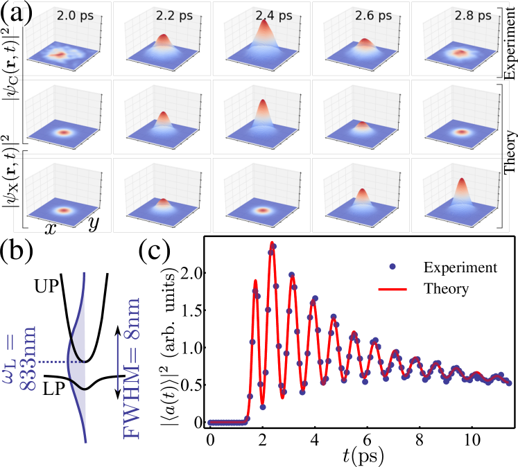
Figure 1: (Color online) (a) Oscillations observed experimentally in the cavity field and reproduced theoretically in both the cavity and exciton fields. (b) The Lower (LP) & Upper (UP) Polaritons excited by a Gaussian pulse which overlap with the branches determines the effective state created in the system. (c) The dynamics can be reduced to that of $|\langle a(t)\rangle|^{2}$ alone and described quantitatively by the theory.

In this Letter, thanks to significant progress in both the quality of the structures and in the laboratory state of the art, we have been able to both observe and provide a full control of the microcavity polariton Rabi dynamics. This brings microcavities one step further as platforms to control and engineer various states of light-matter coupling. We can span from Rabi oscillating configurations to eigenstate superpositions, and control them by optical pulses that can amplify or switch states, thereby achieving the same type of coherent control recently reported in mechanical systems Faust et al. (2013), but fully optically and with over nine orders of magnitude gain in speed. The data offers a perfect quantitative agreement with a fundamental model of light-matter coupling of two bosonic fields, that allows us to pin down the underlying dynamics and explain which factors play which role and to which extent, at the highest level of precision ever attained in a microcavity, thus making such systems even more suitable for engineering and applications.

A typical experimental observation is shown in Fig. 1(a): the cavity field oscillates after its excitation by a $100\text{\,}\mathrm{fs}$ long and $8\text{\,}\mathrm{nm}$ energy broad pulse impinging on both branches, as sketched in Fig. 1(b). The basic interpretation is straightforward: by exciting both branches, the system is prepared as a bare state and, not being an eigenstate, oscillates between its two components. Since polaritons are extended objects, the oscillations is between two fields, localized in a Gaussian of width a few tenths of a $\mu$m given by the exciting laser. This provides us with the first observation of the beatings of a “light-matter drum”. Such a striking dynamics can be accessed thanks to our ultrafast imaging technique based on homodyne interferometric detection, described in a previous work Dominici et al. (2013). This allows us to observe the subpicosecond Rabi oscillations in the direct emission from the exciton-polariton fluid through the coherent fraction $|\psi_{a}(\mathbf{r},t)|^{2}$ of the cavity field in both space $\mathbf{r}$ and time $t$. We used a good quality sample ($\mathrm{Q}\approx 14\,000$), providing a cavity lifetime ($\tau_{a}=$5\text{\,}\mathrm{ps}$$) and an exciton lifetime ($\tau_{b}=$1\text{\,}\mathrm{ns}$$) much longer than the Rabi period, estimated from the coupling strength $g\approx$5.3\text{\,}\mathrm{meV}$$ as $800\text{\,}\mathrm{fs}$. The coupling itself is obtained from the $3\text{\,}\mathrm{nm}$ Rabi splitting between the Lower Polariton (LP) and Upper Polariton (UP) branches. The power is set to excite polaritons at a low enough density, in order to maintain their bosonic properties in the linear regime.

Both the photon-field $\psi_{a}$ dynamics of the experiment and the complementary exciton field $\psi_{b}$, not accessible experimentally, can be recovered by the usual polariton field equations Ciuti and Carusotto (2005) (cf. Supplementary sm ). As expected, the exciton field forms as the photon field vanishes before it is revived as the excitations flow back from excitons into photons again. Limiting to cases with no momentum, although the wavefunction components have a spread in both real and reciprocal spaces, the system is linear and there is no dynamics imparted by the spatial degree of freedom. The dynamics can therefore be reduced to zero-dimension between two single harmonic modes, and the oscillations are fully captured through the simpler order parameters $\langle a(t)\rangle=\int\psi_{a}(\mathbf{r},t)d\mathbf{r}$, accessible experimentally, and $\langle b(t)\rangle=\int\psi_{b}(\mathbf{r},t)d\mathbf{r}$. This is shown in Fig. 1(c) as points, now for the full duration of the experiment. Twelve oscillations are clearly resolved until $t=$12\text{\,}\mathrm{ps}$$. Theoretically, the hamiltonian is reduced to simply $H_{0}=\hbar\omega_{0}({a^{\dagger}}a+{b^{\dagger}}b)+\hbar g({a^{\dagger}}b+a{b^{\dagger}})$, with coupling strength $g$ between the photonic mode $a$ and the emitter annihilation operator $b$, both following Bose algebra and at energy $\omega_{0}$ (resonant case), supplemented with $H_{\Omega}=\sum_{c=a,b}P_{c}(t)e^{i\omega_{\mathrm{L}}t}e^{i\phi_{c}}{c^{\dagger}}+\mathrm{h.c.}$ This is the most general case of coherent and resonant excitation, with coupling to both fields and allowing for a relative phase, which is necessary to reproduce the data. Although the excitation is an optical laser shone directly on the cavity, which is often described theoretically as a cavity-only coupling term Carusotto and Ciuti (2004); Ciuti and Carusotto (2005); Cancellieri et al. (2010), it is clear on physical grounds that such a general form may be required instead, since the exciton field would still be excited without the cavity so it is natural that part of the excitation is shared between the latter and the Quantum Well (QW). While it has little consequence for the single-pulse excitation, this will be crucial when dealing with coherent control by a second pulse. This prepares states of the type of Eq. (2), i.e., classical states that should not be confused with quantum superpositions of the type of Eq. (1) Demirchyan et al. (2014), which would be extremely difficult to realize and maintain even for small values of $|\alpha|^{2}$ and $|\beta|^{2}$. Regardless of the magnitude of pumping, the coherent excitation of two linearly coupled oscillators cancels completely the entanglement of the polariton Fock states to produce factorizable states, in any basis. By integrating Schrödinger’s equation $i\hbar\partial_{t}\psi=H\psi$, one easily finds the closed-form expression for $\alpha(t)$ and $\beta(t)$ under the dynamics of $H=H_{0}+H_{\Omega}$ sm . For the case of an initial state $\left|\alpha_{0}\right\rangle\left|\beta_{0}\right\rangle$, $\left|\psi(t)\right\rangle$ reduces to:

$$\left|\alpha_{0}\cos(gt)-i\beta_{0}\sin(gt)\right\rangle\left|-i\alpha_{0}\sin(gt)+\beta_{0}\cos(gt)\right\rangle\,.$$ (3)

This describes two quantum oscillators, swinging like any other of their classical counterparts, and that mixes features of the bare states (which amplitudes oscillate), with those of the polaritons (with no oscillations of their amplitudes). From the observation of the oscillation alone, it is therefore difficult to capture the true dynamics at play. This is where a theoretical model is needed to shed light on the hidden features Laussy et al. (2009). As we are going to show, the contrast of the oscillation is not due to decoherence between the UP and LP, but to a combination of the short lifetime of the UP and of the effective state realized by the pulsed excitation.

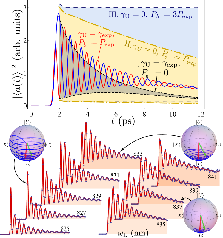
Figure 2: (Color online) Various states created in the system by varying the pulse energy and their evolution on the Bloch sphere, showing the systematic relaxation towards the LP. In inset, the full exciton-photon dynamics reconstructed theoretically for the case $\omega_{\mathrm{L}}=$829\text{\,}\mathrm{nm}$$ and variations (showing the envelope of the oscillations only) when removing the effect of the exciton reservoir (I, black dashed), removing the effect of polariton dephasing (II, dotted-dashed yellow) and removing both (III, long-dashed blue). $P_{\mathrm{exp}}$ and $\gamma_{\mathrm{exp}}$ are the fitted values for the experiment.

While the core of the physics is contained in the wavefunction $\left|\psi\right\rangle$ of the coupled oscillators under the dynamics of $H$, we have to take into account dephasing and decay to describe any experiment with some degree of accuracy. These are mainly due to the bare state lifetimes (with decay rates $\gamma_{a,b}$ for the photon/exciton, respectively), which are also present in most light-matter coupled systems. In QW microcavities, additional sources of dephasing are present for the UP, which is well known to be much less visible than its LP counterpart Baumberg et al. (1998); Skolnick et al. (2000). A contribution from the exciton reservoir has also been suggested in several works, even under coherent excitation Vishnevsky et al. (2012); Wouters et al. (2013). However, no direct measurement of its contribution, nor its true nature (coherent or incoherent) has been clearly reported until now. We can address this issue by including an UP dephasing rate $\gamma_{\mathrm{U}}$ and an incoherent excitonic pumping rate $P_{b}$. Indeed, both terms are required to reproduce the data at the level of accuracy we report. Such terms turn the pure state wavefunction into a density matrix $\rho$ ruled by a master equation. The theory is standard and is given in the Supplementary material sm . In this case, the complex amplitudes of the oscillators can also be derived in closed-form expressions. The experimental modulus square of the cavity amplitude can then be fitted by the model and other observables reconstructed from the theory. The fit provides an essentially perfect agreement with the data, as seen in the figures.

By shifting the laser energy to weight more on one branch than the other, as done for the series displayed in Fig. 2(a), different states can be prepared, that are all equally well accounted for by the theory for the same system parameters. Note also that both the dynamics of the pulse as well as the subsequent free oscillations is described within the same model. From the theory fitting the experimental $|\langle a(t)\rangle|^{2}$, we gain access to the entire dynamics of oscillations, also of the exciton field $|\langle b(t)\rangle|^{2}$, but even further, of the phases $\langle a(t)\rangle$ and $\langle b(t)\rangle$ and the total excitations $\langle({a^{\dagger}}a)(t)\rangle$ and $\langle({b^{\dagger}}b)(t)\rangle$ and, in fact, of the full state as a whole through the density matrix $\rho$. This allows us to reconstruct the full dynamics, as done in Fig. 2 for the joint exciton-photon oscillations of the experiment (case of $827\text{\,}\mathrm{nm}$ excitation), and see the effect of the various factors involved. For instance, the impact of the reservoir is seen in the case I (in dashed black line, from now on plotting only the envelope of the Rabi oscillations for clarity) where it has been set to zero. Its effect is small but is needed to reproduce the data quantitatively. The main detrimental actor is the UP dephasing rate $\gamma_{\mathrm{U}}$, which, if set to zero, considerably opens the envelope of oscillations (case II, blue dashed-dotted line). Interestingly, the incoherent reservoir extends the lifetime of the oscillations as shown in case II and even more so in case III (long dashed line) where an higher pumping rate than that of the experiment brings the oscillations well into the nanosecond timescale, as proposed in Ref. Demirchyan et al. (2014), although, as already noted, this is for normal mode coupling oscillations that cannot be used to engineer a qubit.

The coherent amplitudes of any two-level system can be mapped on the Bloch sphere as $\langle a\rangle/\sqrt{|\langle a\rangle|^{2}+|\langle b\rangle|^{2}}=\cos(\theta/2)$ and $\langle b\rangle/\sqrt{|\langle a\rangle|^{2}+|\langle b\rangle|^{2}}=\sin(\theta/2)\exp(i\phi)$ with $\theta$ and $\phi$ the azimuthal and radial angles of polar coordinates, respectively. Such trajectories from our experiment are shown for three cases in Fig. 2, corresponding to predominant UP excitation, equal weight of the branches and predominant LP excitation. It is clearly seen in the first case how the pulse swings the coupled oscillators towards the upper state and, in all cases, how the system quickly reaches the LP. This is the clearest observation to date of one of the most important assumptions of microcavity polariton physics: the UP is unstable and the system relaxes towards the lower branch, even though it retains strong-coupling. In the model, this UP dephasing rate $\gamma_{\mathrm{U}}$, could be either an escape rate (like a lifetime due to, e.g., scattering to high-$k$ exciton states), a pure dephasing rate, or a combination of boths, as only their sum enters in the equation of the coherent fraction. The result also shows that although the impinging laser is very wide in energy, it is possible to prepare the polariton condensate in a largely tunable range, from almost entirely upper-polaritonic (at least for short times) to almost entirely lower-polaritonic (also the state at long-times), passing by purely photonic and/or excitonic, these two states constantly oscillating between each other.

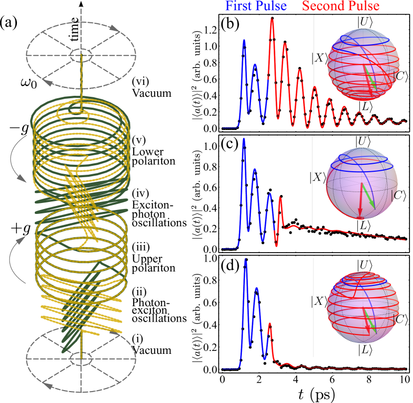
Figure 3: (Color online) (a) Succession of various dynamical evolutions in time of the cavity (dashed yellow) and the exciton (green) complex amplitudes (here with fixed modulus) that can be passed from one to the other with an appropriate pulse excitation. Normal mode-coupling features a $\pi/2$ dephasing in both time and optical phase and oscillate radially while polaritons oscillate circularly. Furthermore, they oscillate jointly and against (resp. $\pi$ out-of-phase with each other and with) the rotating frame in the case of a LP (resp. UP). (b–e) Experimental realization (points) and theoretical fit (solid curve) of three two-pulses excitation, showing (b) amplification, (c) transition from an exciton-photon Rabi oscillation to a LP and (d) field annihilation.

With such an accurate command of the system, we are able to time precisely the arrival of a second pulse and perform a comprehensive coherent control on the coupled dynamics. For a coupling of the laser to the cavity only, this would be achieved for most operations by sending the control pulse when the cavity field is empty and the condensate fully excitonic. Injecting a second fully photonic pulse in optical (resp. anti-optical) phase with the exciton, for instance, creates an UP (resp. LP). It is convenient to represent such a dynamics with the joint photon and exciton fields’ complex phases, as shown in Fig. 3(a) for a sequence of basic operations through pulsed excitation that bring the system from (i) the vacuum and (vi) back passing by a condensate of (ii) photons, (iii) UPs, (iv) excitons and (v) LPs. The photon and exciton condensates are defined as such right after the pulse only since, not being eigenstates, they enter the oscillating regime. In the rotating frame of the bare modes at frequency $\omega_{0}$, the light-matter dynamics is a simple oscillation along the radius with a combined offset of $\pi/2$ both in time and optical phase: the cavity oscillates horizontally while the exciton oscillates vertically and when one reaches its maximum, the other is at the origin. In contrast, the LP and UP condensates do not oscillate radially but circularly, since they are free modes that subtract and add, respectively, their free energy to that of the rotating frame. An animation of this dynamics is given in the Supplementary Material sm .

In the actual experiment, where the laser couples to both fields, one merely needs to correct for the corresponding proportions but the concept is otherwise the same. A first pulse triggers the Rabi oscillations, since our pulse is broad in energy and always initiate a dominant photon or exciton fraction. However, with a second pulse, although still broad, we can refine the state by providing the complementary of the sought target. Figure 3(b) shows a simple case of Rabi amplification, where the same cycle is restarted by the pulse. Figure 3(c) shows the case where a bare state is transformed into a LP, therefore switching off the oscillations. While it has not been practical with our setup to send more than two pulses, there is no fundamental difficulty in doing so and in principle one can implement all the wished steps to prepare any given state right after the pulses. Another case of interest is complete field annihilation, by sending a pulse out-of-phase both in amplitude and in optical phase. This produces, by destructive interferences, the vacuum, as shown in Fig. 3(d). All these cases demonstrate the possibility to do coherent control of the strong light-matter coupling dynamics. Here too, the theory still provides an essentially perfect agreement to the data. Similar prospects at the single-particle level would perform genuine quantum information processing, but this lies beyond the scope of this work.

In conclusion, we showed the tremendous control that can be obtained on the light-matter coupling in microcavities, for which we reported the first imaging of its spatio-temporal evolution. This allowed us to spell out with a precision never achieved before for polaritons both the excitation scheme and the various components involved in the dynamics (dephasing, reservoirs, etc.) We demonstrated the reservoir-induced lifetime enhancement recently proposed Demirchyan et al. (2014) and performed coherent control on the polariton state. Such results are a milestone to turn these systems into devices, with future prospects such as optical gates or their single-particle counterpart now clearly in sight. Immediate extensions suggested by this work are—beyond getting to the single-particle limit—to couple to the spatial degree of freedom with packets imparted with momentum or diffusing, and involve nonlinearities at higher pumpings.

Funding by the ERC POLAFLOW and the IEF SQUIRREL is acknowledged.

Ultrafast control of Rabi oscillations in a polariton condensate :
Supplementary Material.

In this supplementary material, we provide details on the theoretical model, the nature of the state realized in the experiment and the problem of its visualization, the effect of pure dephasing, some limiting analytical solutions and additional fitted data.

I Rabi oscillations between two extended spatial fields

Polaritons in the linear regime implement the physics of two-coupled Schrödinger equations Laussy (2012):

$$i\hbar\partial_{t}\psi_{a}(\mathbf{r},t) =-\frac{\hbar^{2}\nabla^{2}\psi_{a}(\mathbf{r},t)}{2m_{a}}+\hbar g\psi_{b}(\mathbf{r},t)\,,$$ (S1a)

$$3i\hbar\partial_{t}\psi_{b}(\mathbf{r},t) =-\frac{\hbar^{2}\nabla^{2}\psi_{b}(\mathbf{r},t)}{2m_{b}}+\hbar g\psi_{b}(\mathbf{r},t)\,.$$ (S1b)

Each coupled field (cavity photon and exciton) serves as a potential for the other. Here $m_{a,b}$ are the cavity photon and exciton masses, respectively, $g$ their coupling strength, and we are ignoring dissipation for a while. Interestingly, such a simple equation has to the best of our knowledge no known analytical solution. While the coupling can give rise to a complicated dynamics Colas and Laussy (2014), when the diffusion is small and in the linear regime, the phenomenology is simply that of two fields beating at the Rabi frequency. In our experiments, we have provided the first observation of the dynamics of such a “drum of light-and-matter”, cf. Fig. 1(a) of the main text, and our ability to control some of its modes of motion. The Supplementary Video I-SpaceTimeRabiOscillation.avi mov (a) shows the dynamics along the diameter (along a 1D cut of the 2D spatial dynamics) and time for the pulsed excitation at $831\text{\,}\mathrm{nm}$.

In our configuration, where the space dynamics plays no substantial role, it can be averaged over to retain only the key variables that capture the dynamics, namely:

$$\langle a(t)\rangle=\int\psi_{a}(\mathbf{r},t)\,d\mathbf{r}\quad\mathrm{and}\quad\langle b(t)\rangle=\int\psi_{b}(\mathbf{r},t)\,d\mathbf{r}\,,$$ (S2)

in which case the dynamics becomes that of two coupled quantum harmonic oscillators, with commutation relation $[c,{c^{\dagger}}]=1$ for both $c=a,b$, and Hamiltonian (at resonance):

$$H=\hbar\omega_{a}({a^{\dagger}}a+{b^{\dagger}}b)+\hbar g\left({a^{\dagger}}b+a{b^{\dagger}}\right)\,.$$ (S3)

II Hamiltonian dynamics of two linearly coupled oscillators

While the dynamics of two linearly coupled oscillators is extremely simple from a classical perspective, it can become tricky when shifting to the quantum point of view. In addition to the various patterns of oscillations, just as in the classical case, one has to consider the plethora of quantum states that can set them in motion (or not, in cases of eigenstate superpositions). Already for pure states, the wavefunction needs an infinite set of complex coefficients $\alpha_{nm}(t)$ to be fully specified, say in the basis of Fock states $\left|nm\right\rangle$ with $n$ quanta of excitations in oscillator $a$ and $m$ in oscillator $b$, since:

$$\left|\psi(t)\right\rangle=\sum_{n,m=0}^{\infty}\alpha_{nm}(t)\left|nm\right\rangle\,.$$ (S4)

While as much information is necessary to describe genuinely quantum states López Carreño et al. (2014), most of it is redundant for those that have a classical counterpart. For instance, coherent states can be reduced to two complex numbers only:

$$\left|\psi(t)\right\rangle=\left|\alpha(t)\right\rangle\left|\beta(t)\right\rangle\,.$$ (S5)

This is essentially the case of our experiment since the system is excited resonantly by a laser pulse, that creates a coherent state, and it is found a-posteriori by the analysis that dephasing has a small effect given the large populations involved and the short duration of the experiment, resulting in states that remain essentially fully coherent throughout (cf. Section VI).

Adding the excitation scheme as:

$$H_{\Omega}=\sum_{c=a,b}P_{c}(t)e^{i\omega_{\mathrm{L}}t}e^{i\phi_{c}}{c^{\dagger}}+\mathrm{h.c.}$$ (S6)

one can find by straightforward algebra the wavefunction at all later times $t$ under the dynamics of Eq. (S3), starting from the initial condition:

$$\left|\psi(t=0)\right\rangle=\left|\alpha_{0}\right\rangle\left|\beta_{0}\right\rangle\,,$$ (S7)

for any $\alpha_{0}$, $\beta_{0}\in\mathbf{C}$ (possibly zero), to be Eq. (S5) with $\alpha(t)$ and $\beta(t)$ given by:

$$\gamma(t)= \gamma_{0}\cos(gt)-i\bar{\gamma}_{0}\sin(gt)$$ (S8)

$$- G^{+}\exp(-igt)\left(\mathrm{erfi}\left(\frac{it_{1}+\tau^{+}}{\sqrt{2}\sigma}\right)-\mathrm{erfi}\left(\frac{-i(t-t_{1})+\tau^{+}}{\sqrt{2}\sigma}\right)\right)$$

$$\mp G^{-}\exp(igt)\left(\mathrm{erfi}\left(\frac{it_{1}+\tau^{-}}{\sqrt{2}\sigma}\right)-\mathrm{erfi}\left(\frac{-i(t-t_{1})+\tau^{-}}{\sqrt{2}\sigma}\right)\right)$$

with $\gamma$ a notation for either $\alpha$ or $\beta$ with the convention that $\bar{\alpha}=\beta$ and $\bar{\beta}=\alpha$, where we have also defined:

$$G^{\pm}= \frac{1}{4}\exp\left(-\frac{\tau^{\pm}(2it_{1}+\tau^{\pm})}{2\sigma^{2}}\right)(P_{a}\pm P_{b}\exp(i\phi))\,,$$ (S9a)

$$\tau^{\pm}= \sigma^{2}(\mp g+\omega_{l})\,.$$ (S9b)

We have assumed the case of a Gaussian pulse $P_{c}(t)=P_{c}e^{i\phi_{c}}\exp(-(t-t_{1})^{2}/\sigma^{2})/(\sigma\sqrt{2\pi})$ with $\phi=\phi_{b}$ and $\phi_{a}=0$ with no loss of generality. This is the key physics at play in our experiment, and we now consider it in more details.

A first important clarification in the light of a recently published proposal Demirchyan et al. (2014) is that the state that is created following such an excitation is a factorizable product of coherent states of the type (S5), and not a quantum superposition of “macroscopically occupied orthogonal states”. It is true that any Fock state of polaritons is in a such quantum superposition, starting with the building blocks of one-particle states:

$$\|1,0\rrangle =\cos\theta\left|0,1\right\rangle-\sin\theta\left|1,0\right\rangle\,,$$ (S10a)

$$\|0,1\rrangle =\sin\theta\left|0,1\right\rangle+\cos\theta\left|1,0\right\rangle\,,$$ (S10b)

writing $\left|n,m\right\rangle$ as a shortcut for $\left|n\right\rangle\left|m\right\rangle$ the pure state with $n$ photons and $m$ excitons, and $\|n,m\rrangle$ the pure state with $n$ lower polaritons and $m$ upper polaritons. Regardless of the quantum nature of these one-particle states, however, coherent superpositions of them wash out the entanglement and result in coherent states, in any basis. For instance, a coherent state of lower polaritons:

$$\|\alpha,0\rrangle=e^{-|\alpha|^{2}/2}\sum_{n=0}^{\infty}\frac{\alpha^{n}}{\sqrt{n!}}\|n,0\rrangle\,,$$ (S11)

is a product of coherent states of photons and excitons:

$$\|\alpha,0\rrangle =e^{-\frac{|\alpha|^{2}}{2}}\sum_{n=0}^{\infty}\frac{\alpha^{n}}{\sqrt{n!}}\sum_{k=0}^{n}\sqrt{{n\choose k}}\cos^{k}\theta\sin^{n-k}\theta\left|k,n-k\right\rangle\,,$$

$$=\left|\alpha\cos\theta,\alpha\sin\theta\right\rangle\,.$$ (S12)

It is therefore useless for actual quantum information processing, describing an essentially classical phenomenon, although it can have some value to simulate in a controlled classical environment a model qubit Spreeuw and Woerdman (1993).

If one leaves aside the pulse preparation in Eq. (S8) to consider directly the coherent state $\left|\alpha_{0}\right\rangle\left|\beta_{0}\right\rangle$ as the initial condition, the solution reads simply:

$$\left|\psi(t)\right\rangle=\\ \left|\alpha_{0}\cos(gt)-i\beta_{0}\sin(gt)\right\rangle\left|-i\alpha_{0}\sin(gt)+\beta_{0}\cos(gt)\right\rangle\,.$$ (S13)

Two extreme cases are of interest: on the one hand, $\alpha_{0}=\mp\beta_{0}$, in which case the dynamics becomes

$$\left|\psi(t)\right\rangle=\left|\alpha_{0}e^{\pm igt}\right\rangle\left|\mp\alpha_{0}e^{\pm igt}\right\rangle\,,$$ (S14)

corresponding to the freely propagating lower$\|-\sqrt{2}\alpha e^{igt},0\rrangle$ and upper $\|0,\sqrt{2}\alpha e^{-igt}\rrangle$ polariton condensates, respectively. On the other hand, for $\alpha$ nonzero and $\beta=0$ (or vice versa):

$$\left|\psi(t)\right\rangle=\left|\alpha_{0}\cos(gt)\right\rangle\left|-i\alpha_{0}\sin(gt)\right\rangle\,,$$ (S15)

corresponding to Rabi oscillations (here we remind that we use such a qualification as a convenience and in accord with common usage to describe what really is normal-mode coupling oscillations) between the two fields. Polariton states of the type (S13) oscillate in a circle in the counter-rotating (resp. rotating) frame for the lower (resp. upper) polariton case (in the non-rotating frame they oscillate faster, resp. slower, by a factor $g$ over the optical frequency $\omega_{a}$, with $g\ll\omega_{a}$), the two fields being in phase (resp. $\pi$ out of phase). In contrast, states of the type (S15) oscillate radially and perpendicularly, the two fields being $\pi/2$ out-of-phase. The general case combines these two types of motions and results in an elliptical oscillation in phase-space, therefore with a reduced contrast of the oscillations. This is is precisely what happens in our experiment: the oscillations are not full-amplitude not because of decoherence that dephase the coupling, as in the case of genuine Rabi oscillations, but because the state has a strong polaritonic component. We come back to the problem of visualizing this dynamics in Section IV, although with the solution Eqs. (S5—S9), we have provided a complete solution to the problem. Before illustrating particular cases of interest, in next Section, we generalize them to include the effect of dissipation.

III Dissipative dynamics of two linearly coupled oscillators

The Hamiltonian is not enough to quantitatively describe a polariton experiment, that has various sources of decay. This turns, to begin with, the wavefunction into a density matrix ruled by von Neumann equation:

$$\dot{\rho}=\frac{i}{\hbar}\left[\rho,H\right]+\mathcal{L}\rho,$$ (S16)

with $\mathcal{L}\rho$ the Lindblad super-operator which for a generic operator $c$ reads:

$$\mathcal{L}_{c}\rho=2c\rho{c^{\dagger}}-{c^{\dagger}}c\rho-\rho{c^{\dagger}}c\,,$$ (S17)

and in our model takes the form del Valle (2010):

$$\mathcal{L}\rho=\frac{\gamma_{a}}{2}\mathcal{L}_{a}\rho+\frac{\gamma_{b}}{2}\mathcal{L}_{b}\rho+\frac{\gamma_{\mathrm{U}}^{\mathrm{R}}}{2}\mathcal{L}_{u}\rho+\frac{\gamma_{\mathrm{U}}^{\phi}}{2}\mathcal{L}_{{u^{\dagger}}u}\rho+\frac{P_{b}e^{-\gamma_{P_{b}}t}}{2}\mathcal{L}_{{b^{\dagger}}}\rho\,,$$ (S18)

where $\gamma_{a(b)}$ are the modes $a$ and $b$ radiative lifetimes, respectively, $\gamma_{\mathrm{U}}^{R}$ and $\gamma_{\mathrm{U}}^{\phi}$ the radiative and pure dephasing rates for the upper polariton $u=(a+b)/\sqrt{2}$ and $P_{b}e^{-\gamma_{P_{b}}}t$ the incoherent pumping rate from an exciton reservoir with lifetime $\gamma_{P_{b}}$ (we will also introduce late $l=(a-b)/\sqrt{2}$). Such a description is at a high abstract level but a full microscopic description would be so complex that it would be impossible without any phenomenological simplification of this type given the numerical state of the art and the basic physics that nevertheless eventually takes place.

Here again, most of the information encoded in the density matrix is not-needed and the dynamics can be reduced to much fewer variables. To fit the data, since only $|\langle a(t)\rangle|^{2}$ is accessible experimentally, it is enough to calculate the dynamics of $\langle a(t)\rangle$, which only requires that of $\langle b(t)\rangle$. For the general case of two-pulses excitations, it is therefore enough to solve numerically their coupled set of equations:

$$\partial_{t}\langle a(t)\rangle =-i(\frac{P_{a}^{(1)}\,e^{i\phi_{1}}\,e^{-\frac{1}{2}(\frac{t-t_{1}}{\sigma_{1}})^{2}}}{\sqrt{2\pi}\sigma_{1}}+\frac{P_{a}^{(2)}\,e^{i\phi_{2}}\,e^{-\frac{1}{2}(\frac{t-t_{2}}{\sigma_{2}})^{2}}}{\sqrt{2\pi}\sigma_{2}})+\frac{1}{4}(-2\gamma_{a}-\gamma_{\mathrm{U}}+4i\,\omega_{\mathrm{L}})\langle a(t)\rangle-\frac{1}{4}(4i\,g+\gamma_{\mathrm{U}})\langle b(t)\rangle,$$ (S19a)

$$\partial_{t}\langle b(t)\rangle =-i(\frac{P_{b}^{(1)}e^{-\frac{1}{2}(\frac{t-t_{1}}{\sigma_{1}})^{2}}}{\sqrt{2\pi}\sigma_{1}}+\frac{P_{b}^{(2)}\,e^{-\frac{1}{2}(\frac{t-t_{2}}{\sigma_{2}})^{2}}}{\sqrt{2\pi}\sigma_{2}})-\frac{1}{4}(4i\,g+\gamma_{\mathrm{U}})\langle a(t)\rangle+\frac{1}{4}(2P_{b}e^{-\gamma_{P_{b}}\,t}H(t-t_{1})-2\gamma_{b}-\gamma_{\mathrm{U}}+4i\omega_{\mathrm{L}})\langle b(t)\rangle,$$ (S19b)

with the vacuum as initial condition, that is, $\langle a(0)\rangle=\langle b(0)\rangle=0$, and $P_{c}^{(i)}$ the first, $i=1$, and second, $i=2$, pulse coupling to the cavity, $c=a$, and exciton field, $c=b$. Equations (S19) are those that fit all the data reported in this work. By setting to zero the second pulse, $P_{a}^{(2)}=P_{b}^{(2)}=0$, we describe the case of one pulse excitation. In the case where the exciton reservoir has infinite lifetime, $\gamma_{P_{b}}=0$, this can be integrated analytically although the expression is too heavy to be written there. Making the further simplification to dispense from the pulse dynamics and considering the initial state injected instead, Eq. (S7), we can reduce the dynamics to a simple form that captures most of the phenomenology:

$$\langle a(t)\rangle =\begin{aligned} &\Bigg{[}a_{0}\cosh(\frac{1}{4}Rt)-\left(\frac{b_{0}G+a_{0}\Gamma}{R}\right)\sinh(\frac{1}{4}Rt)\Bigg{]}\exp(-\frac{1}{4}\gamma t)\,,\end{aligned}$$ (S20a)

$$\langle b(t)\rangle =\begin{aligned} &\Bigg{[}b_{0}\cosh(\frac{1}{4}Rt)+\left(\frac{-a_{0}G+b_{0}\Gamma}{R}\right)\sinh(\frac{1}{4}Rt)\Bigg{]}\exp(-\frac{1}{4}\gamma t)\,,\end{aligned}$$ (S20b)

where we have introduced:

$$\gamma= \gamma_{a}+\gamma_{b}+\gamma_{\mathrm{U}}-P_{b}\,,$$ (S21a)

$$\Gamma= P_{b}-\gamma_{b}+\gamma_{a}\,,$$ (S21b)

$$G= i4g+\gamma_{\mathrm{U}}\,,$$ (S21c)

$$R= \sqrt{G^{2}+\Gamma^{2}}\,,$$ (S21d)

and, since only the sum of radiative decay $\gamma_{\mathrm{U}}^{\mathrm{R}}$ and pure dephasing $\gamma_{\mathrm{U}}^{\mathrm{\phi}}$ of the upper polariton plays a role in the coherent dynamics, the total upper polariton dephasing rate:

$$\gamma_{\mathrm{U}}=\gamma_{\mathrm{U}}^{\mathrm{R}}+\gamma_{\mathrm{U}}^{\phi}\,.$$ (S22)

The solution Eqs. (S20–S21) relates to that of Eqs. (S5–S9) in that it includes dissipation (both radiative lifetime and pure dephasing of the upper polariton) as well as the incoherent pumping from the reservoir (assumed constant) but neglects the coherent excitation (the two pulses), considering an initial state instead. It also provides the dynamics of $\langle a(t)\rangle$ and $\langle b(t)\rangle$ only but makes no restriction on the quantum state, that can be any density matrix, including states with no classical counterparts, whereas Eqs. (S5–S9) provides the full quantum state but in a case where it is at all times in the form Eq. (S5). Therefore, they provide two closed-form solutions in two limiting cases. Of course they agree in their region of overlap.

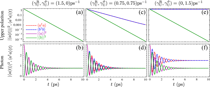
Figure S1: (Color online) Effect of dephasing on the polariton population. The three cases shown in three columns for two different initial conditions (rows) keep the total rate $\gamma_{\mathrm{U}}=$3\text{/}2\text{\,}{\mathrm{ps}}^{-1}$$ constant but balances radiative and pure dephasing from Eq. (S22) as indicated in the header of each column. The evolution of the coherent (solid green & purple) and total, i.e., coherent+incoherent (dashed red & blue) populations of exciton and photon are shown as a function of time, starting from a condensate of upper polaritons (upper row) and of photons (lower row). The coherent fraction is the same, and looses its particle either radiatively or transferred to the incoherent fraction.

IV Visualization of the dynamics

We now discuss the problem of the visualization of the polariton dynamics. At a basic level, the problem seems innocuous enough, as it deals with oscillations, which are essentially captured by their amplitude and phase. For two fields, this means two complex numbers, i.e., four variables. Two complex numbers can be mapped onto the Bloch sphere if dropping their relative phase, which indeed can be done with no loss of generality. The state of the oscillator at any given time $t$ can thus be positioned on a sphere with polar coordinates defined as:

$$\theta=\frac{\langle a\rangle}{\sqrt{|\langle a\rangle|^{2}+|\langle b\rangle|^{2}}}\quad\mathrm{and}\quad\phi=\frac{\langle b\rangle}{\sqrt{|\langle a\rangle|^{2}+|\langle b\rangle|^{2}}}\,,$$ (S23)

possibly keeping its radius normalized to one, as we do in this work for clarity. This is the representation we have adopted whenever we display a trajectory on the sphere, with always the convention that:

1. The north pole corresponds to the Upper Polariton (noted $\left|\mathrm{U}\right\rangle$),

2. The south pole corresponds to the Lower Polariton (noted $\left|\mathrm{L}\right\rangle$),

3. The right-side point on the equator corresponds to the Cavity Photon (noted $\left|\mathrm{C}\right\rangle$),

4. The left-side point on the equator corresponds to the Exciton (noted $\left|\mathrm{X}\right\rangle$).

Here it is important to keep in mind that throughout, and regardless of the notation, this maps a state of the type Eq. (S5), specifically, $\left|\alpha\right\rangle\left|\beta\right\rangle$, and not a qubit nor a superposition of the states. The possibility to map to the same sphere either the classical state of two coherent fields or the quantum state of a qubit $\cos(\theta/2)\left|0\right\rangle\left|1\right\rangle+e^{i\phi}\sin(\theta/2)\left|1\right\rangle\left|0\right\rangle$, can allow for some classical simulation of a qubit, which may have some value, but cannot, obviously, substitute for it in an actual quantum computer. We leave the analysis of quantum oscillations to another text López Carreño et al. (2014) and focus here on the case of interest for the experiment.

The Bloch sphere representation is the most concise one, but it says nothing about the incoherent fraction. In our experiment, it turns out that the states remain highly coherent throughout, and there is no need to consider the dynamics of the incoherent part that grows due to dephasing and incoherent pumping.

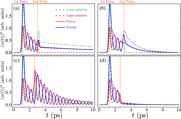
Figure S2: (Color online) Two-pulses experiment (cf. Fig. 3 of the main text) as seen through all the theoretical variables: bare states in solid and eigenstates in dashed lines. The experimentally available variable is the photon field, in red. The three cases correspond to: (a) switching-off of the Rabi oscillation by bringing the state into a lower-polariton condensate, (b) revival of the oscillations and (c) annihilation of the field.

However, to be comprehensive, since we still need the relative phase information of both fields, and to put the current results in perspective with future ones with smaller number of particles, where more general states can be realized, we now discuss a more comprehensive picture, namely, the Husimi representation Husimi (1940). It is given for two coherent fields by:

$$Q(\alpha,\beta)=\left\langle\alpha\beta\right|\rho\left|\alpha\beta\right\rangle\,,$$ (S24)

and can be represented in its reduced form for each fields in two panels, juxtaposing $Q(\alpha)=\int Q(\alpha,\beta)\,d\beta$ and $Q(\beta)=\int Q(\alpha,\beta)\,d\alpha$. When it is a product of coherent states, the factorization is exact and no information is lost, in which case it is equivalent to the complex phase representation that we have used in the text, cf. Fig. 3(a), merely replacing the point by a Gaussian cloud of mean square deviation $1/2$ and whose amplitude and phase are otherwise given by the population and phase of the oscillator. This is arguably the most convenient way to visualize the polariton dynamics of normal-mode coupling, particularly if it can be animated. In the supplementary video II-RabiOscillations.mp4 mov (b), we provide the same dynamics as Fig. 3(a), namely, the sequence of pulses that bring the systems into the successive states:

1. vacuum,

2. excitation of a photon condensate,

3. transfer to an upper polariton condensate,

4. transfer to an exciton condensate,

5. transfer to a lower polariton condensate,

6. annihilation and return to the vacuum.

This is the theoretical, ideal version of what the experiment realizes with one operation at a time, since the time-window available to us is not currently large enough to chain up various pulses. However the proof of principle has been fully demonstrated.

Although in our case the fitting implies that the system remains highly coherent at all times, before we turn to the details of the dynamics in this case, we contrast it with cases where dephasing plays a more important role. In Fig. S1, we show the dynamics of the system prepared in the upper polariton state (which is the state that suffers the most from dephasing) for three different balancing of the total dephasing rate $\gamma_{\mathrm{U}}$ given by Eq. (S22)—that is the parameter accessible to the experiment—into radiative upper polariton decay $\gamma_{\mathrm{U}}^{\mathrm{R}}$ and pure dephasing of the upper polariton $\gamma_{\mathrm{U}}^{\phi}$. The calculations, done in this case with the master equation, involved only a few particles, so that the effect of dephasing be noticeable. In the experiment, where it is estimated as orders of magnitudes higher, the impact would not be significant on the timescales involved. To keep the discussion as simple as possible, we consider upper polariton dephasing only and as initial condition, coherent states of upper polaritons or of photons, each with 3 particles at $t=0$. One can see how the breakdown of polariton dephasing into radiative decay and pure dephasing results in different evolution of the quantum state, although the coherent fraction (solid line) remains the same, being dependent only on the total dephasing rate (S22). Only in the case where there is some level of pure dephasing do the two cases differ. Compare in particular the first and third columns, where the polaritons are either lost (first column) or transferred to the incoherent fraction (third column). In the latter case, the population remain constant when starting as a polariton or becomes so when the polariton fraction has vanished to leave a fully incoherent mixture. The movie corresponding to the case (c) in the Husimi representation is provided in the Supplementary Material as III-RabiDephasing.avi mov (c). The Gaussian cloud spreads into a ring as it rotates, corresponding to the washing out of the phase. This together with the various modes of oscillations mov (a) give a hint as to what the complete polariton dynamics look like, when adding to such dephasing also the radiative decay and Rabi oscillations.

V Two-pulses control

As we have seen in the previous Section, one value of the theory is to unveil the full dynamics and gain access to variables not reachable by the experiment. In Fig. S2, we show the representation for the two-pulses dynamics of the experiment (cf. Fig. 3 of the main text where the experimental points are also shown), here supplemented with the observables made accessible by the theory, namely also $|\langle b(t)\rangle|^{2}$ (solid blue) the amplitude squared of the exciton condensate and $|\langle u(t)\rangle|^{2}$ the upper polariton (dashed purple) and $|\langle l(t)\rangle|^{2}$ the lower polariton (dashed green).

This representation gives another look at the physics already discussed. In the first case, panel (a), the state is brought from an oscillating exciton-photon dynamics into a lower polariton, therefore switching-off the oscillations. The lifetime is also changed as a result. In the second case, panel (b), the transfer is to the upper polariton instead (a case not achieved in the experiment). The phenomenology is the same but with a faster decay rate. In case (c), the oscillation is revived and carries on Rabi-oscillating beyond our experimental window. This shows in particular how the upper polariton is, again, the limiting factor, although, from the fit, it appears it is easily set in motion and populated, more than the lower polariton itself. Since it decays so quickly, ultimately the system is driven into a lower polariton state only, regardless of its excitation at initial time. Here again, we must stress that the decay of the contrast of oscillations with time is therefore not due to dephasing, but because upper polaritons are lost at a greater rate, making the system increasingly lower-polaritonic, which is a non-oscillating state. In the last panel, (d), we provide the clear observation that the field is annihilated altogether in this configuration where both the Rabi and the optical phases of the second pulses are in opposition, which is not apparent on the Bloch sphere that enforces the normalization.

VI Fitting of the data

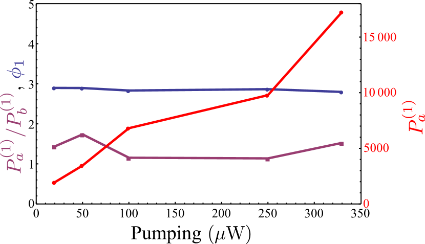
Figure S3: (Color online) Best fitting numerical value for the pumping parameters $P_{a}^{(1)}$ (red), right axis, and the ratio $P_{a}^{(1)}/P_{b}^{(1)}$, roughly constant, and relative phase $\phi_{A}$ (left axis), in the pumping series.

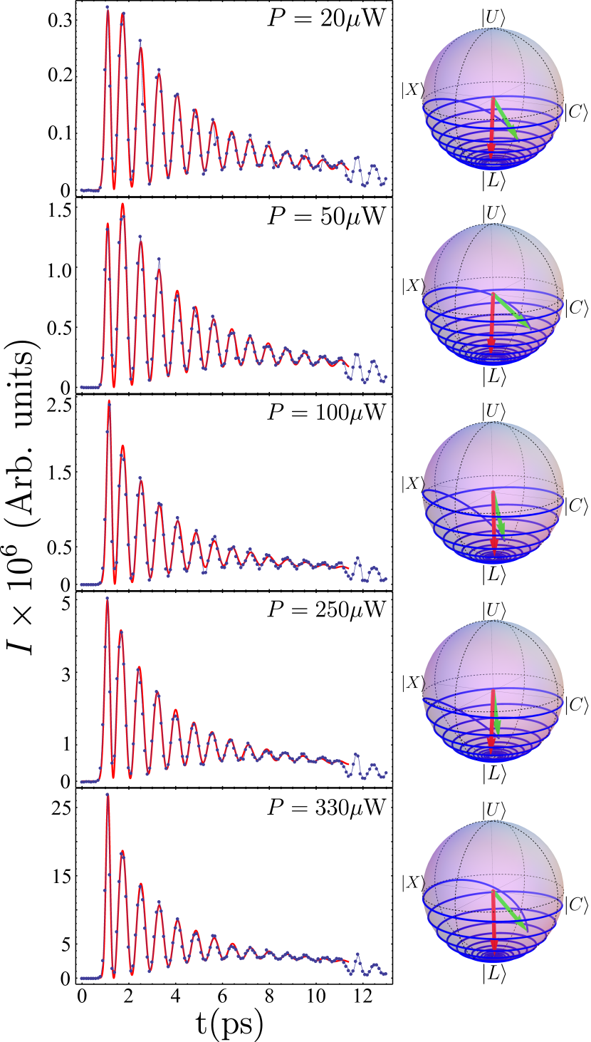
Figure S4: (Color online) Power serie experiment. The evolution of the system is presented for different powers. On the graphs, the blue points are the experimental datas, linked by straight lines to guid the eye. The red curves are obtained with the fitting process. The corresponding quantum state is represented on the Bloch Sphere, the initial state being represented by the green arrow and the final state by the red one.

In this last Section, we provide additional material on the fitting of the experimental data by the theory, i.e., by Eqs. (S19).

Parameters have been optimized through a multi-pass fitting procedure that first adjust all parameters and then constrain the system parameters, i.e., those specific to the sample—which are listed in Table 1 for the $\omega_{\mathrm{L}}$ series provided in the text—and fit only over those of the pulse in a global-fitting procedure over various experiments. The fit is not sensitive to the exciton lifetime as long as it is very large and we have fixed it to $1\text{\,}\mathrm{ns}$, typical of a reservoir exciton. This provides an essentially perfect fit to the data with very few completely free parameters, most of them being kept fixed in the global fit, and those of the pulse varying as dictated by the experiment ($\omega_{\mathrm{L}}$). This leaves only $P_{c}^{(i)}$ and $\phi_{c}$, $c=a$, $b$ and $i=1$, $2$, as the truly free parameters, providing useful information on how the laser couples to the microcavity.

Parameters	Physical Meaning	Best Fit
$g$	Coupling Strength	2.65 $\textrm{ps}^{-1}$
$\gamma_{a}$	Cavity decay rate	0.2 $\textrm{ps}^{-1}$
$\gamma_{b}$	Exciton decay rate	0.001 $\textrm{ps}^{-1}$
$\gamma_{\mathrm{U}}$	Upper polariton dephasing rate	0.43 $\textrm{ps}^{-1}$
$P_{b}$	Exciton reservoir pumping rate	0.11 $\textrm{ps}^{-1}$
$\gamma_{P_{b}}$	Exciton reservoir decay rate	0.01 $\textrm{ps}^{-1}$

Table 1: System parameters and their best fit values for the energy series experiment (varying $\omega_{\mathrm{L}}$, cf. Fig. 2 of the main text). The same parameters apply for the pumping series, only with $\gamma_{\mathrm{U}}=1/$0.41\text{\,}\mathrm{ps}$$

In addition to the laser energy series, presented in the main text, we have also studied the pumping dependence. The results we have reported lie in the low excitation regime to retain the linear features, and we are going to show the stability of such a regime over one order of magnitude pumping. At higher powers, deviations appear that will be analyzed separately. At very high powers, a new physics altogether emerge with spectacular phenomenology such as the observation of a long-living, ultrasharp backjet Dominici et al. (2013). Figure S4 shows the data and its fit by the model as the power of the laser is tuned from $20\text{\,}\mathrm{\SIUnitSymbolMicro W}$ to $330\text{\,}\mathrm{\SIUnitSymbolMicro W}$ while the excitation energy is kept constant at $\omega_{\mathrm{L}}=$829\text{\,}\mathrm{nm}$$. The same multi-pass fitting procedure was used for the power serie and provides again an essentially perfect fit of the experiment. The corresponding parameters, summarized in the Table 1, present an excellent agreement with the ones obtained previously for the energy serie (cf. see Table 1 in the main text). Figure S3 displays the numerical values for $P_{a}^{(1)}$ (red) and $\phi_{A}$ (blue) as well as the ratio $P_{a}^{(1)}/P_{b}^{(1)}$ (purple). The fitting values increase roughly linearly with pumping, as expected since this is precisely the variable that is tuned experimentally. This also indicates how the laser couples to the system. This is an information that is not easily obtained and from which we gather that the laser couples in equal part to the photon than to the exciton, both being almost in optical antiphase. That the coupling of the laser to the microcavity is not only through the cavity but also to the exciton is important for coherent control in particular but may have implications in other aspect of polariton physics. The coupling is found to be independent of pumping, as shown by the constant ratio and phase, which leads to an initial state on the sphere in the same vicinity, see the green arrows on the different sphere in Fig. S3. This also shows that the reservoir grows linearly with pumping, since the rate is fixed. The shape of the Rabi oscillations after the pulse remains independent of the pumping, only scaling in total particle numbers. The apparent different contrast with pumping is an artifact due to the larger contribution of the pulse at higher pumping, dwarfing the rest of the free dynamics.

References

- Rabi (1937) I. I. Rabi, Phys. Rev. 51, 652 (1937).
- Schumacher (1995) B. Schumacher, Phys. Rev. A 51, 2738 (1995).
- Nielsen and Chuang (2000) M. A. Nielsen and I. L. Chuang, Quantum computation and quantum information (Cambridge University Press, 2000).
- Spreeuw and Woerdman (1993) R. Spreeuw and J. Woerdman, Progress in Optics 31, 263 (1993).
- Faust et al. (2013) T. Faust, J. Rieger, M. J. Seitner, J. P. Kotthaus, and E. M. Weig, Nat. Phys. 9, 485 (2013).
- Zhu et al. (1990) Y. Zhu, D. J. Gauthier, S. E. Morin, Q. Wu, H. J. Carmichael, and T. W. Mossberg, Phys. Rev. Lett. 64, 2499 (1990).
- Khitrova et al. (2006) G. Khitrova, H. M. Gibbs, M. Kira, S. W. Koch, and A. Scherer, Nat. Phys. 2, 81 (2006).
- Matthews et al. (1999) M. R. Matthews, B. P. Anderson, P. C. Haljan, D. S. Hall, M. J. Holland, J. E. Williams, C. E. Wieman, and E. A. Cornell, Phys. Rev. Lett. 83, 3358 (1999).
- Vasa et al. (2013) P. Vasa, W. Wang, R. Pomraenke, M. Lammers, M. Maiuri, C. Manzoni, G. Cerullo, and C. Lienau, Nat. Photon. 7, 128 (2013).
- Spreeuw (1998) R. J. C. Spreeuw, Found. Phys. 28, 361 (1998).
- Spreeuw (2001) R. J. C. Spreeuw, Phys. Rev. A 63, 062302 (2001).
- Dragoman and Dragoman (2004) D. Dragoman and M. Dragoman, Quantum-Classical Analogies, The Frontiers Collection (Springer, 2004).
- Spreeuw et al. (1990) R. J. C. Spreeuw, N. J. van Druten, M. W. Beijersbergen, E. R. Eliel, and J. P. Woerdman, Phys. Rev. Lett. 65, 2642 (1990).
- Okamoto et al. (2013) H. Okamoto, A. Gourgout, C.-Y. Chang, K. Onomitsu, I. Mahboob, E. Y. Chang, and H. Yamaguchi, Nat. Phys. 9, 480 (2013).
- Hennessy et al. (2007) K. Hennessy, A. Badolato, M. Winger, D. Gerace, M. Atature, S. Gulde, S. Fălt, E. L. Hu, and A. Ĭmamoḡlu, Nature 445, 896 (2007).
- Weisbuch et al. (1992) C. Weisbuch, M. Nishioka, A. Ishikawa, and Y. Arakawa, Phys. Rev. Lett. 69, 3314 (1992).
- Kavokin et al. (2011) A. Kavokin, J. J. Baumberg, G. Malpuech, and F. P. Laussy, Microcavities (Oxford University Press, 2011), 2nd ed.
- Carusotto and Ciuti (2013) I. Carusotto and C. Ciuti, Rev. Mod. Phys. 85, 299 (2013).
- Kasprzak et al. (2006) J. Kasprzak, M. Richard, S. Kundermann, A. Baas, P. Jeambrun, J. M. J. Keeling, F. M. Marchetti, M. H. Szymanska, R. André, J. L. Staehli, et al., Nature 443, 409 (2006).
- Amo et al. (2009a) A. Amo, D. Sanvitto, F. P. Laussy, D. Ballarini, E. del Valle, M. D. Martin, A. Lemaître, J. Bloch, D. N. Krizhanovskii, M. S. Skolnick, et al., Nature 457, 291 (2009a).
- Amo et al. (2009b) A. Amo, J. Lefrère, S. Pigeon, C. Adrados, C. Ciuti, I. Carusotto, R. Houdré, E. Giacobino, and A. Bramati, Nat. Phys. 5, 805 (2009b).
- Liew et al. (2008) T. C. H. Liew, A. V. Kavokin, and I. A. Shelykh, Phys. Rev. Lett. 101, 016402 (2008).
- Amo et al. (2010) A. Amo, T. C. H. Liew, C. Adrados, R. Houdré, E. Giacobino, A. V. Kavokin, and A. Bramati, Nat. Photon. 4, 361 (2010).
- Amo et al. (2011) A. Amo, S. Pigeon, D. Sanvitto, V. G. Sala, R. Hivet, I. Carusotto, F. Pisanello, G. Leménager, R. Houdré, E. Giacobino, et al., Science 332, 1167 (2011).
- Baumberg et al. (2008) J. J. Baumberg, A. V. Kavokin, S. Christopoulos, A. J. D. Grundy, R. Butté, G. Christmann, D. D. Solnyshkov, G. Malpuech, G. B. H. von Högersthal, E. Feltin, et al., Phys. Rev. Lett. 101, 136409 (2008).
- Schneider et al. (2013) C. Schneider, A. Rahimi-Iman, N. Y. Kim, J. Fischer, I. G. Savenko, M. Amthor, M. Lermer, A. Wolf, L. Worschech, V. D. Kulakovskii, et al., Nature 497, 348 (2013).
- Ballarini et al. (2013) D. Ballarini, M. D. Giorgi, E. Cancellieri, R. Houdré, E. Giacobino, R. Cingolani, A. Bramati, G. Gigli, and D. Sanvitto, Nat. Comm. 4, 1778 (2013).
- Norris et al. (1994) T. Norris, J.-K. Rhee, C.-Y. Sung, Y. Arakawa, M. Nishioka, and C. Weisbuch, Phys. Rev. B 50, 14663 (1994).
- Savona and Weisbuch (1996) V. Savona and C. Weisbuch, Phys. Rev. B 54, 10835 (1996).
- Wang and Vyas (1995) C. Wang and R. Vyas, Phys. Rev. A 51, 2516 (1995).
- Marie et al. (1999) X. Marie, P. Renucci, S. Dubourg, T. Amand, P. L. Jeune, J. Barrau, J. Bloch, and R. Planel, Phys. Rev. B 59, 2494(R) (1999).
- Brunetti et al. (2006) A. Brunetti, M. Vladimirova, D. Scalbert, M. Nawrocki, A. V. Kavokin, I. A. Shelykh, and J. Bloch, Phys. Rev. B 74, 241101(R) (2006).
- Boulier et al. (2014) T. Boulier, M. Bamba, A. Amo, C. Adrados, A. Lemaitre, E. Galopin, I. Sagnes, J. Bloch, C. Ciuti, E. Giacobino, et al., Nat. Comm. 5 (2014).
- Silva et al. (2014) B. Silva, A. González Tudela, C. Sánchez Muñoz, D. Ballarini, G. Gigli, K. W. West, L. Pfeiffer, E. del Valle, D. Sanvitto, and F. P. Laussy, arXiv:1406.0964 (2014).
- Dominici et al. (2013) L. Dominici, D. Ballarini, M. D. Giorgi, E. Cancellieri, B. Silva, A. Bramati, G. Gigli, F. Laussy, and D. Sanvitto, arXiv:1309.3083 (2013).
- Ciuti and Carusotto (2005) C. Ciuti and I. Carusotto, Phys. Stat. Sol. B 242, 2224 (2005).
- (37) See supplementary material.
- Carusotto and Ciuti (2004) I. Carusotto and C. Ciuti, Phys. Rev. Lett. 93, 166401 (2004).
- Cancellieri et al. (2010) E. Cancellieri, F. M. Marchetti, M. H. Szymanska, and C. Tejedor, Phys. Rev. B 82, 224512 (2010).
- Demirchyan et al. (2014) S. Demirchyan, I. Chestnov, A. Alodjants, M. Glazov, and A. Kavokin, Phys. Rev. Lett. 112, 196403 (2014).
- Laussy et al. (2009) F. P. Laussy, E. del Valle, and C. Tejedor, Phys. Rev. B 79, 235325 (2009).
- Baumberg et al. (1998) J. J. Baumberg, A. Armitage, M. S. Skolnick, and J. S. Roberts, Phys. Rev. Lett. 81, 661 (1998).
- Skolnick et al. (2000) M. S. Skolnick, V. N. Astratov, D. M. Whittaker, A. Armitage, M. Emam-Ismael, R. M. Stevenson, J. J. Baumberg, J. S. Roberts, D. G. Lidzey, T. Virgili, et al., J. Lum. 87, 25 (2000).
- Vishnevsky et al. (2012) D. V. Vishnevsky, D. D. Solnyshkov, N. A. Gippius, and G. Malpuech, Phys. Rev. B 85, 155328 (2012).
- Wouters et al. (2013) M. Wouters, T. K. Paraïso, Y. Léger, R. Cerna, F. Morier-Genoud, M. T. Portella-Oberli, and B. Deveaud-Plédran, Phys. Rev. B 87, 045303 (2013).

References

- Laussy (2012) F. Laussy, Exciton-polaritons in microcavities (Springer Berlin Heidelberg, 2012), vol. 172, chap. 1. Quantum Dynamics of Polariton Condensates, pp. 1–42, ISBN 978-3-642-24186-4.
- Colas and Laussy (2014) D. Colas and F. Laussy, unpublished (2014).
- mov (a) See file I-SpaceTimeRabiOscillation.avi, Supplementary Movie.
- López Carreño et al. (2014) J. López Carreño, J. Restrepo Cuartas, E. del Valle, and F. Laussy, Unpublished (2014).
- Demirchyan et al. (2014) S. Demirchyan, I. Chestnov, A. Alodjants, M. Glazov, and A. Kavokin, Phys. Rev. Lett. 112, 196403 (2014).
- Spreeuw and Woerdman (1993) R. Spreeuw and J. Woerdman, Progress in Optics 31, 263 (1993).
- del Valle (2010) E. del Valle, Microcavity Quantum Electrodynamics (VDM Verlag, 2010).
- Husimi (1940) K. Husimi, Proc. Phys. Math. Soc. Jpn 22, 264 (1940).
- mov (b) See file II-RabiOscillations.avi, Supplementary Movie.
- mov (c) See file III-RabiDephasing.avi, Supplementary Movie.
- Dominici et al. (2013) L. Dominici, D. Ballarini, M. D. Giorgi, E. Cancellieri, B. Silva, A. Bramati, G. Gigli, F. Laussy, and D. Sanvitto, arXiv:1309.3083 (2013).