Integrable anyon chains: from fusion rules to face models
to effective field theories

Peter E. Finch    Michael Flohr    Holger Frahm Institut für Theoretische Physik, Leibniz Universität Hannover, Appelstraße 2, 30167 Hannover, Germany
Abstract

Starting from the fusion rules for the algebra $SO(5)_{2}$ we construct one-dimensional lattice models of interacting anyons with commuting transfer matrices of ‘interactions round the face’ (IRF) type. The conserved topological charges of the anyon chain are recovered from the transfer matrices in the limit of large spectral parameter. The properties of the models in the thermodynamic limit and the low energy excitations are studied using Bethe ansatz methods. Two of the anyon models are critical at zero temperature. From the analysis of the finite size spectrum we find that they are effectively described by rational conformal field theories invariant under extensions of the Virasoro algebra, namely $\mathcal{W}B_{2}$ and $\mathcal{W}D_{5}$, respectively. The latter contains primaries with half and quarter spin. The modular partition function and fusion rules are derived and found to be consistent with the results for the lattice model.

I Introduction

Starting with Bethe’s study of the spin-$\frac{1}{2}$ Heisenberg chain integrable models in low dimensions have provided important insights into the peculiarities of correlated many-body systems subject to strong quantum fluctuations Bethe (1931); Baxter (1982); Korepin et al. (1993); Essler et al. (2005), e.g. the appearance of quasi-particles with exotic properties such as fractional quantum numbers and with unusual braiding statistics. In a wider context these anyons appear as excitations in topologically ordered systems without a local order parameter. Realizations for such topological quantum liquids are the fractional Hall states Laughlin (1983) and two-dimensional frustrated quantum magnets Moessner and Sondhi (2001); Balents et al. (2002); Kitaev (2006). Non-Abelian anyons can also be realized as local modes with zero energy at junctions of spin-orbit coupled quantum wires through the ’topological’ Kondo effect Béri and Cooper (2012); Altland et al. (2013, 2014). Additional interest in these objects arises from the fact that non-Abelian anyons are protected by their topological charge which makes them potentially interesting as resources for quantum computation Kitaev (2003); Nayak et al. (2008).

A class of integrable models describing interacting non-Abelian anyons in one dimension can be obtained from two dimensional classical lattice systems with interactions round the face (IRF) such as the restricted solid on solid (RSOS) models Andrews et al. (1984) in their Hamiltonian limit. The critical RSOS models are lattice realizations of the unitary minimal models Friedan et al. (1984); Huse (1984) and the family of commuting operators generated by their transfer matrices contains Hamiltonians for Fibonacci or, more generally, $SU(2)_{k}$ anyons with nearest neighbor interactions Feiguin et al. (2007). Recently, extensive studies of these anyons and their higher spin variants subject to different interactions or in different geometries have led to the identification of a variety of critical phases and the corresponding conformal field theories from finite size spectra obtained numerically Trebst et al. (2008); Gils et al. (2009, 2013); Ludwig et al. (2011); Pfeifer et al. (2012).

Several approaches exist for the construction of integrable IRF models: integrable generalizations of the RSOS models have been obtained by means of the fusion procedure Date et al. (1986). Alternatively, the correspondence between integrable IRF models and vertex models Pasquier (1988); Roche (1990) (or, equivalently, anyon chains and quantum spin chains) with an underlying symmetry of a quasi-triangular Hopf algebra can be exploited to construct anyonic quantum chains Finch (2013); Finch and Frahm (2013). Finally, new models can be defined by labeling the local height variables on neighboring sites of the lattice by adjacent roots in the A-D-E Dynkin diagrams or, more generally by primary fields of a general rational conformal field theory related through the corresponding fusion algebra Pasquier (1987); Gepner (1993). For these models to be integrable one has to find a parameterization of the Boltzmann weights for the configuration allowed around a face of the lattice which satisfies the Yang-Baxter equation. This can be achieved by Baxterization of a representation of the braid group associated to the symmetries of the underlying system.

In the following we apply this last approach to construct four integrable quantum chains of a particular type of anyons responsible for the non-Fermi liquid correlations predicted in the topological Kondo effect Altland et al. (2013, 2014). Specifically, we consider anyons satisfying the fusion rules of $SO(5)_{2}$. Below we will see that – as might be expected for a model based on $SO(5)=B_{2}$ – the anyonic quantum chains are related to IRF models with height variables outside the A-D-E classification. The integrability of the models is established by construction of representations of the Birman-Murakami-Wenzl (BMW) algebra in terms of anyonic projection operators. The spectra of these models are determined by Bethe ansatz methods and we identify the ground state and low lying excitations. Two of the models can be related to the six-vertex model in the ferromagnetic and anti-ferromagnetic gapped regime, respectively, by means of a Temperley-Lieb equivalence. From the analysis of the finite size spectrum the other two integrable points are found to be critical with the low energy sector described by unitary rational conformal field theories (RCFTs) with extended symmetries associated to the Lie algebras $B_{2}=SO(5)$ and $D_{5}=SO(10)$, respectively. To present our results in a self-contained way, some general facts on the classification and spectral data of the relevant minimal models of Casimir-type $\mathcal{W}$-algebras are included in Appendix B. For the anti-ferromagnetic anyon chain we propose a modular invariant partition function in terms of the Virasoro characters of the irreducible highest weight representations of the $\mathcal{W}D_{5}(9,10)$ RCFT. The $\mathcal{S}$-matrix and fusion rules of this CFT are given in Appendix C.

II $SO(5)_{2}$ anyons

Algebraically, anyonic theories can be described by braided tensor categories Kitaev (2006); Bonderson (2007); Preskill (2004). A braided tensor category consists of a collection of objects $\{\psi_{i}\}$ (including an identity) equipped with a tensor product (fusion rules),

$\displaystyle\psi_{a}\otimes\psi_{b}$ $\displaystyle\cong$ $\displaystyle\bigoplus_{c}N_{ab}^{c}\psi_{c}$

where $N_{ab}^{c}$ are non-negative integers. In the special case $N_{ab}^{c}\in\{0,1\}$ it is called multiplicity free. Below we shall use a graphical representation of ’fusion states’ of the anyon model where vertices

may occur provided that $\psi_{c}$ appears in the fusion of $\psi_{a}$ and $\psi_{b}$. We require associativity in our fusion i.e.

$\displaystyle(\psi_{a}\otimes\psi_{b})\otimes\psi_{c}$ $\displaystyle\cong$ $\displaystyle\psi_{a}\otimes(\psi_{b}\otimes\psi_{c}),$

which is governed by $F$-moves, also referred to as generalized $6j$-symbols,

$a$ $e$ $b$ $c$ $d$ $=\sum_{d^{\prime}}(F^{abc}_{e})^{d}_{d^{\prime}}$ $a$ $e$ $b$ $c$ $d^{\prime}$ (1)

For more than three objects different decompositions of the fusion can be related by distinct sequences of $F$-moves. Their consistency for arbitrary number of factors is guaranteed by the Pentagon equation satisfied by the $F$-moves.

There also must be a mapping that braids two objects,

$\displaystyle R:\psi_{a}\otimes\psi_{b}$ $\displaystyle\rightarrow$ $\displaystyle\psi_{b}\otimes\psi_{a}.$

Note that while fusion is commutative, states of the system may pick up a phase $R^{ab}_{c}$ under braiding. Graphically this is represented by

$a$ $b$ $c$ $=\quad R^{ab}_{c}\quad$ $b$ $a$ $c$ (2)

For a consistent anyon theory braids have to commute with fusion and satisfy the Yang-Baxter relation. Both properties follow from the Hexagon equation for $F$- and $R$-moves.

In this paper we consider a system of particles which satisfy the fusion rules for $SO(5)_{2}$ shown in Table 1.

$\otimes$ $\psi_{1}$ $\psi_{2}$ $\psi_{3}$ $\psi_{4}$ $\psi_{5}$ $\psi_{6}$
$\psi_{1}$ $\psi_{1}$ $\psi_{2}$ $\psi_{3}$ $\psi_{4}$ $\psi_{5}$ $\psi_{6}$
$\psi_{2}$ $\psi_{2}$ $\psi_{1}\oplus\psi_{5}\oplus\psi_{6}$ $\psi_{3}\oplus\psi_{4}$ $\psi_{3}\oplus\psi_{4}$ $\psi_{2}\oplus\psi_{5}$ $\psi_{2}$
$\psi_{3}$ $\psi_{3}$ $\psi_{3}\oplus\psi_{4}$ $\psi_{1}\oplus\psi_{2}\oplus\psi_{5}$ $\psi_{2}\oplus\psi_{5}\oplus\psi_{6}$ $\psi_{3}\oplus\psi_{4}$ $\psi_{4}$
$\psi_{4}$ $\psi_{4}$ $\psi_{3}\oplus\psi_{4}$ $\psi_{2}\oplus\psi_{5}\oplus\psi_{6}$ $\psi_{1}\oplus\psi_{2}\oplus\psi_{5}$ $\psi_{3}\oplus\psi_{4}$ $\psi_{3}$
$\psi_{5}$ $\psi_{5}$ $\psi_{2}\oplus\psi_{5}$ $\psi_{3}\oplus\psi_{4}$ $\psi_{3}\oplus\psi_{4}$ $\psi_{1}\oplus\psi_{2}\oplus\psi_{6}$ $\psi_{5}$
$\psi_{6}$ $\psi_{6}$ $\psi_{2}$ $\psi_{4}$ $\psi_{3}$ $\psi_{5}$ $\psi_{1}$
Table 1: The fusion rules for $SO(5)_{2}$ anyons.

This fusion algebra is the truncation of the category of irreducible representations of the quantum group $U_{q}(so(5))$ where $q=\mathrm{e}^{\frac{2i\pi}{5}}$ Bonderson (2007). For the $SO(5)_{2}$ fusion rules there exist four known sets of inequivalent unitary $F$-moves, which can be found by solving the pentagon equations directly or by utilizing the representation theory of $U_{q}(so(5))$. Associated with each set of $F$-moves is a modular $\mathcal{S}$-matrix which diagonalizes the fusion rules (note that the latter may depend on the choice of $F$-moves Bonderson (2007)). We have selected the $F$-moves corresponding to the $S$-matrix

$$\mathcal{S}=\frac{1}{2\sqrt{5}}\left(\begin{array}[]{cccccc}1&2&\sqrt{5}&\sqrt{5}&2&1\\ 2&-2\phi&0&0&2\phi^{-1}&2\\ \sqrt{5}&0&-\sqrt{5}&\sqrt{5}&0&-\sqrt{5}\\ \sqrt{5}&0&\sqrt{5}&-\sqrt{5}&0&-\sqrt{5}\\ 2&-2\phi^{-1}&0&0&2\phi&2\\ 1&2&-\sqrt{5}&-\sqrt{5}&2&1\\ \end{array}\right)$$ (3)

where $\phi=\frac{1+\sqrt{5}}{2}$. With this choice of $F$-moves we have four possible sets (in two mirror pairs) of $R$-moves. For the purposes of this article, however, we do not need to explicitly choose one.

Given a consistent set of rules for the fusion and braiding we can construct a one-dimensional chain of interacting ‘anyons’ with topological charge $\psi_{j}$. First a suitable basis has to be built using fusion paths Moore and Seiberg (1990); Preskill (2004): starting with an auxiliary anyon $\psi_{a_{0}}$ we choose one of the objects appearing in the fusion $\psi_{a_{0}}\otimes\psi_{j}$, say $\psi_{a_{1}}$. The latter is fused to another $\psi_{j}$, and so forth. Recording the irreducible subspace of the auxiliary space and the subsequent irreducible subspaces which appear after fusion we construct basis states

ψjψjψjψjψjψa0ψa1ψa2ψa3ψa1ψa|a0a1a2a1a.\leavevmode\hbox to185.34pt{\vbox to14.63pt{\pgfpicture\makeatletter\hbox{\hskip-14.02638pt\lower-17.27182pt\hbox to0.0pt{\pgfsys@beginscope\pgfsys@invoke{ }\definecolor{pgfstrokecolor}{rgb}{0,0,0}\pgfsys@color@rgb@stroke{0}{0}{0}\pgfsys@invoke{ }\pgfsys@color@rgb@fill{0}{0}{0}\pgfsys@invoke{ }\pgfsys@setlinewidth{0.4pt}\pgfsys@invoke{ }\nullfont\hbox to0.0pt{\pgfsys@beginscope\pgfsys@invoke{ }{{}} \put(30.0,0.0){$\psi_{j}$} \put(60.0,0.0){$\psi_{j}$} \put(90.0,0.0){$\psi_{j}$} \put(150.0,0.0){$\psi_{j}$} \put(180.0,0.0){$\psi_{j}$} \put(0.0,-20.0){$\psi_{a_{0}}$} \put(40.0,-27.0){$\psi_{a_{1}}$} \put(70.0,-27.0){$\psi_{a_{2}}$} \put(100.0,-27.0){$\psi_{a_{3}}$} \put(160.0,-27.0){$\psi_{a_{\mathcal{L}-1}}$} \put(205.0,-20.0){$\psi_{a_{\mathcal{L}}}$} {}{{}}{} {}{}{}\pgfsys@moveto{14.22638pt}{-17.07182pt}\pgfsys@lineto{113.81104pt}{-17.07182pt}\pgfsys@stroke\pgfsys@invoke{ } {}{{}}{} {}{}{}\pgfsys@moveto{119.5015pt}{-17.07182pt}\pgfsys@lineto{125.19196pt}{-17.07182pt}\pgfsys@stroke\pgfsys@invoke{ } {}{{}}{} {}{}{}\pgfsys@moveto{130.88286pt}{-17.07182pt}\pgfsys@lineto{136.57332pt}{-17.07182pt}\pgfsys@stroke\pgfsys@invoke{ } {}{{}}{} {}{}{}\pgfsys@moveto{142.2638pt}{-17.07182pt}\pgfsys@lineto{199.16931pt}{-17.07182pt}\pgfsys@stroke\pgfsys@invoke{ } {}{{}}{} {}{}{}\pgfsys@moveto{32.72049pt}{-2.84544pt}\pgfsys@lineto{32.72049pt}{-17.07182pt}\pgfsys@stroke\pgfsys@invoke{ } {}{{}}{} {}{}{}\pgfsys@moveto{62.59598pt}{-2.84544pt}\pgfsys@lineto{62.59598pt}{-17.07182pt}\pgfsys@stroke\pgfsys@invoke{ } {}{{}}{} {}{}{}\pgfsys@moveto{92.47147pt}{-2.84544pt}\pgfsys@lineto{92.47147pt}{-17.07182pt}\pgfsys@stroke\pgfsys@invoke{ } {}{{}}{} {}{}{}\pgfsys@moveto{152.22243pt}{-2.84544pt}\pgfsys@lineto{152.22243pt}{-17.07182pt}\pgfsys@stroke\pgfsys@invoke{ } {}{{}}{} {}{}{}\pgfsys@moveto{182.09747pt}{-2.84544pt}\pgfsys@lineto{182.09747pt}{-17.07182pt}\pgfsys@stroke\pgfsys@invoke{ } \pgfsys@invoke{\lxSVG@closescope }\pgfsys@endscope{}{}{}\hss}\pgfsys@discardpath\pgfsys@invoke{\lxSVG@closescope }\pgfsys@endscope\hss}}\lxSVG@closescope\endpgfpicture}}\vspace{0.6cm}\hskip 28.45274pt\equiv\left|a_{0}a_{1}a_{2}...a_{\mathcal{L}-1}a_{\mathcal{L}}\right>\,. (4)

Note that the construction implies that any two neighboring labels, $a_{i}a_{i+1}$ must satisfy a local conditions, namely $N_{a_{i},j}^{a_{i+1}}\neq 0$. This local condition can be presented in the form of a graph in which labels which are allowed to be neighbors correspond to adjacent vertices.

For a system with periodic boundary conditions we have to identify $a_{0}$ and $a_{\mathcal{L}}$ (which allows to remove the label $a_{0}$ from the basis states (4)). In this case the Hilbert space of the model can be further decomposed into sectors labeled by topological charges. To measure these charges one inserts an additional anyon of type $\psi_{\ell}$ into the system which is then moved around the chain using (1) and finally removed again Feiguin et al. (2007). The corresponding topological operator $Y_{\ell}$ has matrix elements

$$\left<a_{1}^{\prime}...a_{\mathcal{L}}^{\prime}\right|Y_{\ell}\left|a_{1}...a_{\mathcal{L}}\right>=\prod_{i=1}^{\mathcal{L}}\left(F^{\ell a_{i}^{\prime}j}_{a_{i+1}}\right)^{a_{i}}_{a_{i+1}^{\prime}}\,,\quad\ell=1,\ldots,6\,.$$ (5)

The spectrum of these operators is known: their eigenvalues are given in terms of the matrix elements of the modular $\mathcal{S}$-matrix as $\frac{\mathcal{S}_{k\ell}}{\mathcal{S}_{1\ell}}$ Kitaev (2006).

Local operators acting on the space of fusion paths of the $\psi_{j}$ anyons can be written in terms of projection operators. In terms of the $F$-moves (1) they can be introduced in the following way Feiguin et al. (2007),

pi(b){jjai1aiai+1}\displaystyle p^{(b)}_{i}\left\{\hskip 11.38092pt\leavevmode\hbox to71.53pt{\vbox to20.32pt{\pgfpicture\makeatletter\hbox{\hskip-9.75864pt\lower-17.27182pt\hbox to0.0pt{\pgfsys@beginscope\pgfsys@invoke{ }\definecolor{pgfstrokecolor}{rgb}{0,0,0}\pgfsys@color@rgb@stroke{0}{0}{0}\pgfsys@invoke{ }\pgfsys@color@rgb@fill{0}{0}{0}\pgfsys@invoke{ }\pgfsys@setlinewidth{0.4pt}\pgfsys@invoke{ }\nullfont\hbox to0.0pt{\pgfsys@beginscope\pgfsys@invoke{ }{{}} \put(26.0,5.0){$j$} \put(56.0,5.0){$j$} \put(0.0,-27.0){$a_{i-1}$} \put(40.0,-27.0){$a_{i}$} \put(72.0,-27.0){$a_{i+1}$} {}{{}}{} {}{}{}\pgfsys@moveto{9.95863pt}{-17.07182pt}\pgfsys@lineto{81.09053pt}{-17.07182pt}\pgfsys@stroke\pgfsys@invoke{ } {}{{}}{} {}{}{}\pgfsys@moveto{28.45276pt}{2.84544pt}\pgfsys@lineto{28.45276pt}{-17.07182pt}\pgfsys@stroke\pgfsys@invoke{ } {}{{}}{} {}{}{}\pgfsys@moveto{58.32823pt}{2.84544pt}\pgfsys@lineto{58.32823pt}{-17.07182pt}\pgfsys@stroke\pgfsys@invoke{ } \pgfsys@invoke{\lxSVG@closescope }\pgfsys@endscope{}{}{}\hss}\pgfsys@discardpath\pgfsys@invoke{\lxSVG@closescope }\pgfsys@endscope\hss}}\lxSVG@closescope\endpgfpicture}}\hskip 11.38092pt\right\} =\displaystyle= b(Fai+1ai1jj)baiδbb{jjai1bai+1}\displaystyle\sum_{b^{\prime}}(F^{a_{i-1}jj}_{a_{i+1}})_{b^{\prime}}^{a_{i}}\,\delta_{b}^{b^{\prime}}\left\{\hskip 9.95863pt\leavevmode\hbox to57.31pt{\vbox to20.32pt{\pgfpicture\makeatletter\hbox{\hskip-16.87183pt\lower-17.27182pt\hbox to0.0pt{\pgfsys@beginscope\pgfsys@invoke{ }\definecolor{pgfstrokecolor}{rgb}{0,0,0}\pgfsys@color@rgb@stroke{0}{0}{0}\pgfsys@invoke{ }\pgfsys@color@rgb@fill{0}{0}{0}\pgfsys@invoke{ }\pgfsys@setlinewidth{0.4pt}\pgfsys@invoke{ }\nullfont\hbox to0.0pt{\pgfsys@beginscope\pgfsys@invoke{ }{{}} \put(26.0,5.0){$j$} \put(56.0,5.0){$j$} \put(8.0,-27.0){$a_{i-1}$} \put(47.0,-15.0){$b^{\prime}$} \put(67.0,-27.0){$a_{i+1}$} {}{{}}{} {}{}{}\pgfsys@moveto{17.07182pt}{-17.07182pt}\pgfsys@lineto{73.97734pt}{-17.07182pt}\pgfsys@stroke\pgfsys@invoke{ } {}{{}}{} {}{}{}\pgfsys@moveto{28.45276pt}{2.84544pt}\pgfsys@lineto{43.39027pt}{-7.11319pt}\pgfsys@stroke\pgfsys@invoke{ } {}{{}}{} {}{}{}\pgfsys@moveto{58.32823pt}{2.84544pt}\pgfsys@lineto{43.39027pt}{-7.11319pt}\pgfsys@stroke\pgfsys@invoke{ } {}{{}}{} {}{}{}\pgfsys@moveto{43.39027pt}{-7.11319pt}\pgfsys@lineto{43.39027pt}{-17.07182pt}\pgfsys@stroke\pgfsys@invoke{ } \pgfsys@invoke{\lxSVG@closescope }\pgfsys@endscope{}{}{}\hss}\pgfsys@discardpath\pgfsys@invoke{\lxSVG@closescope }\pgfsys@endscope\hss}}\lxSVG@closescope\endpgfpicture}}\hskip 11.38092pt\right\}
=\displaystyle= ai[(Fai+1ai1jj)bai](Fai+1ai1jj)bai{jjai1aiai+1}.\displaystyle\sum_{a_{i}^{\prime}}\left[\left(F^{a_{i-1}jj}_{a_{i+1}}\right)^{a_{i}^{\prime}}_{b}\right]^{*}\left(F^{a_{i-1}jj}_{a_{i+1}}\right)^{a_{i}}_{b}\left\{\hskip 11.38092pt\leavevmode\hbox to71.53pt{\vbox to20.32pt{\pgfpicture\makeatletter\hbox{\hskip-9.75864pt\lower-17.27182pt\hbox to0.0pt{\pgfsys@beginscope\pgfsys@invoke{ }\definecolor{pgfstrokecolor}{rgb}{0,0,0}\pgfsys@color@rgb@stroke{0}{0}{0}\pgfsys@invoke{ }\pgfsys@color@rgb@fill{0}{0}{0}\pgfsys@invoke{ }\pgfsys@setlinewidth{0.4pt}\pgfsys@invoke{ }\nullfont\hbox to0.0pt{\pgfsys@beginscope\pgfsys@invoke{ }{{}} \put(26.0,5.0){$j$} \put(56.0,5.0){$j$} \put(0.0,-27.0){$a_{i-1}$} \put(40.0,-27.0){$a_{i}^{\prime}$} \put(72.0,-27.0){$a_{i+1}$} {}{{}}{} {}{}{}\pgfsys@moveto{9.95863pt}{-17.07182pt}\pgfsys@lineto{81.09053pt}{-17.07182pt}\pgfsys@stroke\pgfsys@invoke{ } {}{{}}{} {}{}{}\pgfsys@moveto{28.45276pt}{2.84544pt}\pgfsys@lineto{28.45276pt}{-17.07182pt}\pgfsys@stroke\pgfsys@invoke{ } {}{{}}{} {}{}{}\pgfsys@moveto{58.32823pt}{2.84544pt}\pgfsys@lineto{58.32823pt}{-17.07182pt}\pgfsys@stroke\pgfsys@invoke{ } \pgfsys@invoke{\lxSVG@closescope }\pgfsys@endscope{}{}{}\hss}\pgfsys@discardpath\pgfsys@invoke{\lxSVG@closescope }\pgfsys@endscope\hss}}\lxSVG@closescope\endpgfpicture}}\hskip 11.38092pt\right\}\,.

In the second line we have used that the $F$-moves are unitary. For our choice of $SO(5)_{2}$ $F$-moves this can be ensured by choosing a suitable gauge. In terms of the basis states (4) the $p^{(b)}_{i}$ can be written alternatively as

$$p^{(b)}_{i}=\sum_{a_{i-1},a_{i},a_{i}^{\prime},a_{i+1}}\left[\left(F^{a_{i-1}jj}_{a_{i+1}}\right)^{a_{i}^{\prime}}_{b}\right]^{*}\left(F^{a_{i-1}jj}_{a_{i+1}}\right)^{a_{i}}_{b}\left|..a_{i-1}a_{i}^{\prime}a_{i+1}..\right>\left<..a_{i-1}a_{i}a_{i+1}..\right|.$$ (6)

Note that the matrix elements of these operators depend on triples of neighboring labels $a_{i-1}a_{i}a_{i+1}$ in the fusion path but only the middle one may change under the action of the $p^{(b)}_{i}$.

III The $\psi_{3}$-anyon chain

Based on the $SO(5)_{2}$ fusion rules, Table 1, non-trivial models can be defined for $\psi_{2}$ (or, equivalently, $\psi_{5}$) and $\psi_{3}$ ($\psi_{4}$) anyons. In this paper we construct integrable chains of $\psi_{3}$ anyons. The selection rules for neighboring labels in the fusion path (4) displayed in Figure 1. This defines the Hilbert space of the anyon chains.

$\psi_{1}$ $\psi_{2}$ $\psi_{3}$ $\psi_{4}$ $\psi_{5}$ $\psi_{6}$
Figure 1: A graphical representation of allowed neighboring labels in the fusion paths of the $\psi_{3}$ anyon chain. The vertices/nodes of the graphs are the labels of anyons which are connected via an edge if and only if the two anyon labels can appear next to each other.

III.1 Local Hamiltonians

We shall concentrate on models with local interactions given in terms of the projection operators (6). The resulting Hamiltonians are the anyon chain (or face model) analogue of spin chains with nearest neighbor interactions Finch (2013); Pasquier (1988). There are only three non-zero linearly independent projection operators which can be defined on the tensor product $\psi_{3}\otimes\psi_{3}=\psi_{1}\oplus\psi_{2}\oplus\psi_{5}$, i.e.

$$p^{(1)}_{i}+p^{(2)}_{i}+p^{(5)}_{i}=\mathbf{1}\,.$$

Therefore the most general local interaction has a single free coupling parameter

$$h_{i}(\theta)=\cos\left(\frac{\pi}{4}+\theta\right)p^{(2)}_{i}+\sin\left(\frac{\pi}{4}+\theta\right)p^{(5)}_{i}\,,$$ (7)

and the general global Hamiltonian for the anyon chain can be written as

$$\mathcal{H}_{\theta}=\sum_{i}h_{i}(\theta)\,.$$ (8)

Recently, the phase diagram of this model as a function of the parameter $\theta$ has been investigated numerically Finch et al. (2014).

From Table 1, we see that there exists an automorphism of the fusion rules exchanging $\psi_{2}$ and $\psi_{5}$ which allows the construction of a non-local unitary transformation

$$U^{\dagger}\mathcal{H}_{\theta}U=\mathcal{H}_{-\theta}\,.$$ (9)

We also recall that the Hamiltonian commutes with the topological operators (5),

$$\left[\mathcal{H}_{\theta},Y_{\ell}\right]=0$$

for $\theta\in[0,2\pi)$ and $\ell=1,..,6$.

III.2 Points of integrability

In order to establish integrability of the model (8) for particular choices of the parameter $\theta$ it has to be shown that the Hamiltonian is a member of a complete set of commuting operators. This can be done starting from $R$-matrices depending on a parameter acting on the tensor product $\psi_{3}\otimes\psi_{3}$, i.e.

$\displaystyle R(u)$ $\displaystyle=w_{1}(u)\,p^{(1)}+w_{2}(u)\,p^{(2)}+w_{5}(u)\,p^{(5)}$ (10)
$\displaystyle=\sum_{a,b,c,d}W\left(\left.\begin{array}[]{cc}a&b\\ c&d\end{array}\right|u\right)\left|abd\right>\left<acd\right|$

which satisfy the Yang–Baxter equation (YBE)

$$R_{j}(u)R_{j+1}(u+v)R_{j}(v)=R_{j+1}(v)R_{j}(u+v)R_{j+1}(u)\,.$$ (11)

Every solution to this equation defines an integrable statistical model on a square lattice with interactions round a face (or restricted solid-on-solid), see Figure 2.

$W\left(\left.\begin{array}[]{cc}b_{1}&b_{2}\\ a_{1}&a_{2}\end{array}\right|u\right)$ $W\left(\left.\begin{array}[]{cc}b_{2}&b_{3}\\ a_{2}&a_{3}\end{array}\right|u\right)$ $W\left(\left.\begin{array}[]{cc}b_{3}&b_{3}\\ a_{1}&a_{4}\end{array}\right|u\right)$ $W\left(\left.\begin{array}[]{cc}c_{1}&c_{2}\\ b_{1}&b_{2}\end{array}\right|u\right)$ $W\left(\left.\begin{array}[]{cc}c_{2}&c_{3}\\ b_{2}&b_{3}\end{array}\right|u\right)$ $W\left(\left.\begin{array}[]{cc}c_{3}&c_{3}\\ b_{1}&b_{4}\end{array}\right|u\right)$ $a_{1}$ $a_{2}$ $a_{3}$ $a_{4}$ $b_{1}$ $b_{2}$ $b_{3}$ $b_{4}$ $c_{1}$ $c_{2}$ $c_{3}$ $c_{4}$
Figure 2: A two-dimensional lattice of heights with weights placed on faces.

The configurations of this model are labeled by height variables on each node of the lattice with neighboring heights corresponding to adjacent nodes on the graph Figure 1. To each face we assign the Boltzmann weight $W\left(\left.\begin{array}[]{cc}a&b\\ c&d\end{array}\right|u\right)$ from Equation (10) and calculate the total weight of the configuration by taking the product of all face weights. The partition function is given as the sum of total weights over all possible configurations of heights. It is clear from Figure 1 that this model does not correspond to any model within the A-D-E classification Pasquier (1987); Gepner (1993). Likewise, it is known that models of this type can be mapped to loop models Pasquier (1987); Warnaar and Nienhuis (1993), see Figure 3.

$1$ $3$ $5$ $4$ $3$ $2$ $4$ $6$ $2$ $4$ $5$ $4$ $1$ $3$ $5$ $4$ $3$ $2$ $4$ $6$ $2$ $4$ $5$ $4$
Figure 3: Drawing contour lines/domain walls between regions of different heights allows RSOS models to be mapped onto loop models.

As a consequence of the Yang–Baxter equation the face model can be solved using the commuting transfer matrices on the Hilbert space of the periodic anyon chain

$\displaystyle\left<b_{1}...b_{\mathcal{L}}\right|t(u)\left|a_{1}...a_{\mathcal{L}}\right>$ $\displaystyle=\prod_{i=1}^{\mathcal{L}}W\left(\left.\begin{array}[]{cc}b_{i}&b_{i+1}\\ a_{i}&a_{i+1}\end{array}\right|u\right)\,,$ (12)
$\displaystyle\left[t(u),t(v)\right]$ $\displaystyle=0.$

Similar to the topological $Y$-operators, the transfer matrix can be viewed as describing the process of moving an auxiliary anyon around the chain. In this case, however, the braiding is governed by the parameter-dependent $R$-matrix (or, equivalently, the Boltzmann weights) rather than by constants of the underlying category.

Just as there is a natural relationship between two-dimensional vertex models and spin chains there exists a correspondence between this two-dimensional interaction round the face model (IRF) and an anyon chain. Provided that the $R$-matrix degenerates to the identity operator for a particular value $u_{0}$ of the spectral parameter it follows that at $u=u_{0}$ the transfer matrix becomes the shift operator,

$$t(u_{0})\left|a_{1}...a_{\mathcal{L}-1}a_{\mathcal{L}}\right>=\alpha\left|a_{\mathcal{L}}a_{1}...a_{\mathcal{L}-1}\right>\,.$$

This motivates the definition of a momentum operator and Hamiltonian by expanding the transfer matrix around $u_{0}$:

$\displaystyle\mathcal{P}$ $\displaystyle=\frac{1}{i}\ln\left[\frac{t(u_{0})}{\alpha}\right]\,,$ (13)
$\displaystyle\mathcal{H}$ $\displaystyle=\alpha^{\prime}\left.\frac{d}{du}\ln\left[t(u)\right]\right|_{u=u_{0}}+\alpha^{\prime\prime}\mathcal{L}\,.$

For a proper choice of the parameters $\alpha^{\prime}$ and $\alpha^{\prime\prime}$ the local Hamiltonian

$$h=\alpha^{\prime}\left.\frac{d}{du}\ln\left[R(u)\right]\right|_{u=u_{0}}+\alpha^{\prime\prime},$$ (14)

coincides with (7).

To construct points of integrability we construct representations of the Birman-Murakami-Wenzl (BMW) algebra Birman and Wenzl (1989); *Mura87 using the local projection operators (6) occurring in the $\psi_{3}$-anyon model. We define the operators

$\displaystyle E_{j}$ $\displaystyle=\sqrt{5}\,p_{j}^{(1)}\,,$ (15)
$\displaystyle G_{j}$ $\displaystyle=R^{33}_{1}\,p_{j}^{(1)}+R^{33}_{2}\,p_{j}^{(2)}+R^{33}_{5}\,p_{j}^{(5)}$
$\displaystyle=i\left(p_{j}^{(1)}+\mathrm{e}^{\frac{4i\pi}{5}}p_{j}^{(2)}+\mathrm{e}^{-\frac{4i\pi}{5}}p_{j}^{(5)}\right)\,,$

where the $R^{ab}_{c}$ belong to one of the sets of $R$-moves (2). These operators satisfy the relations:

$\displaystyle G_{j}G_{j+1}G_{j}$ $\displaystyle=G_{j+1}G_{j}G_{j+1}$
$\displaystyle E_{j}E_{j\pm 1}E_{j}$ $\displaystyle=E_{j}$
$\displaystyle G_{j}G_{j\pm 1}E_{j}$ $\displaystyle=E_{j}G_{j\pm 1}G_{j}\,=\,E_{j\pm 1}E_{j}$
$\displaystyle G_{j\pm 1}E_{j}G_{j\pm 1}$ $\displaystyle=G_{j}^{-1}E_{j\pm 1}G_{j}^{-1}$
$\displaystyle E_{j}G_{j\pm 1}E_{j}$ $\displaystyle=-iE_{j}$
$\displaystyle G_{j}E_{j}$ $\displaystyle=E_{j}G_{j}\,=\,iE_{j}$
$\displaystyle G_{j}-G_{j}^{-1}$ $\displaystyle=-i\phi(\mathbf{1}-E_{j})$
$\displaystyle E_{j}^{2}$ $\displaystyle=\sqrt{5}E_{j}$

and

$\displaystyle G_{j}G_{j^{\prime}}$ $\displaystyle=G_{j^{\prime}}G_{j}$
$\displaystyle E_{j}E_{j^{\prime}}$ $\displaystyle=E_{j^{\prime}}E_{j}$

for $|j-j^{\prime}|>1$. As mentioned above there exist three other sets of $R$-moves consistent with our choice of the modular $\mathcal{S}$-matrix (3). Using one of these in (15) would be equivalent to replacing $G_{j}$ with either $G_{j}^{-1}$, $U^{\dagger}G_{j}U$ or $U^{\dagger}G_{j}^{-1}U$ with the unitary transformation (9) and modifying the above relations suitably.

The BMW algebra contains a copy of the Temperley-Lieb algebra Temperley and Lieb (1971) as a subalgebra, from which we can construct the solution to the YBE

$\displaystyle R_{j}(u)$ $\displaystyle=\sinh(\gamma+u)\,\mathbf{1}-\sinh(u)\,E_{j},$
$\displaystyle=\sinh(\gamma-u)\,p^{(1)}+\sinh(\gamma+u)\left[p^{(2)}_{j}+p^{(5)}_{j}\right]$

with $\cosh\gamma=\frac{\sqrt{5}}{2}$. Expanding of the resulting transfer matrix around $u_{0}=0$ one obtains the anyon model (8) with $(\alpha^{\prime},\alpha^{\prime\prime})=\pm(\frac{1}{2\sqrt{2}},\frac{1}{2\sqrt{10}})$ for $\theta=0$ and $\pi$. As for other Temperley-Lieb models it can be written as

$$\mathcal{H}_{0,\pi}=\frac{\mp 1}{\sqrt{10}}\sum_{j=1}^{\mathcal{L}}E_{j}+\mathrm{const.}\,.$$

Using the full BMW algebra one can find two additional solutions to the YBE Cheng et al. (1991). One of them is Cheng et al. (1992); Grimm (1994)

$\displaystyle R_{j}(u)=$ $\displaystyle\sinh\left(\frac{7i\pi}{10}\right)\sinh\left(\frac{i\pi}{10}\right)\mathbf{1}+\frac{1}{2}\sinh(u)\left(\mathrm{e}^{\frac{i\pi}{10}-u}G_{j}-\mathrm{e}^{u-\frac{i\pi}{10}}G_{j}^{-1}\right)$ (16)
$\displaystyle=$ $\displaystyle\sinh\left(u+\frac{i\pi}{10}\right)\sinh\left(u+\frac{3i\pi}{10}\right)p^{(1)}_{j}+\sinh\left(u-\frac{i\pi}{10}\right)\sinh\left(u-\frac{3i\pi}{10}\right)p^{(2)}_{j}$
$\displaystyle+\sinh\left(u+\frac{9i\pi}{10}\right)\sinh\left(u+\frac{3i\pi}{10}\right)p^{(5)}_{j}\,.$

This solution leads to integrable points at $\theta=\eta,\eta+\pi$ where $\eta=\mathrm{atan}\left(\frac{1+\sqrt{5}}{4}\right)-\frac{\pi}{4}$. The other $R$-matrix obtained by Baxterization of the BMW representation is related to (16) through the transformation (9) and gives rise to integrable points at $\theta=-\eta,-\eta+\pi$. However, these integrable points are equivalent to the ones they are mapped from and are subsequently omitted from further analysis.

As stated earlier, the weights given by (10) will lead to a solution of the YBE and a commuting transfer matrix (12). It turns out that this transfer matrix belongs to a family of commuting transfer matrices. To define these transfer matrices we present the YBE for face weights

$\displaystyle\sum_{g}W^{\alpha\beta}\left(\left.\begin{array}[]{cc}a&g\\ b&c\end{array}\right|u\right)W^{\alpha\gamma}\left(\left.\begin{array}[]{cc}g&f\\ c&d\end{array}\right|u+v\right)W^{\beta\gamma}\left(\left.\begin{array}[]{cc}a&e\\ g&f\end{array}\right|v\right)$ (17)
$\displaystyle\quad=\quad\sum_{g}W^{\alpha\beta}\left(\left.\begin{array}[]{cc}b&g\\ c&d\end{array}\right|v\right)W^{\alpha\gamma}\left(\left.\begin{array}[]{cc}a&e\\ b&g\end{array}\right|u+v\right)W^{\alpha\beta}\left(\left.\begin{array}[]{cc}e&f\\ g&d\end{array}\right|u\right).$

The general form we use for these face-weights is

$$W^{\alpha\beta}\left(\left.\begin{array}[]{cc}a&b\\ c&d\end{array}\right|u\right)=\sum_{l=1}^{6}w^{\alpha,\beta}_{l}(u)\left[\left(F^{a\beta\alpha}_{d}\right)^{b}_{l}\right]^{*}\left(F^{a\alpha\beta}_{d}\right)^{c}_{l}.$$ (18)

In the case $\alpha=\beta=\gamma=3$ and $w^{3,3}_{l}(u)=w_{l}(u)$, equations (11) and (17) are equivalent. We are able to determine the required set of weights (see Appendix A), such that we have a family of commuting transfer matrices

$\displaystyle\left<b_{1}...b_{\mathcal{L}}\right|t^{(\ell)}(u)\left|a_{1}...a_{\mathcal{L}}\right>$ $\displaystyle=\prod_{i=1}^{\mathcal{L}}W^{\ell 3}\left(\left.\begin{array}[]{cc}b_{i}&b_{i+1}\\ a_{i}&a_{i+1}\end{array}\right|u\right)\,,$ (19)
$\displaystyle\left[t^{(\ell)}(u),t^{(\ell^{\prime})}(v)\right]$ $\displaystyle=0\,,$

for $\ell,\ell^{\prime}=1,\ldots,6$ and $u,v\in\mathbb{C}$. An additional important feature of these transfer matrices is that the limit of each is also a $Y$-operator (5), i.e.

$\displaystyle\lim_{u\rightarrow\pm\infty}t^{(\ell)}(u)$ $\displaystyle=$ $\displaystyle const\times Y_{\ell}\,.$

The appearance of the topological operators as a limit of these transfer matrices is not unexpected as the braiding governed by these weights and the underlying category coincide when $u\rightarrow\pm\infty$.

IV Bethe Ansatz and low energy spectrum

IV.1 The Temperley-Lieb point

The Temperley-Lieb algebra underlying the model at $\theta=0,\pi$ implies that the spectrum of the anyon chain can be related to that of the XXZ spin-1/2 quantum chain with anisotropy $|\Delta|=\cosh\gamma=\frac{\sqrt{5}}{2}$ Temperley and Lieb (1971); Owczarek and Baxter (1987). For the periodic boundary conditions considered here the Temperley-Lieb equivalence implies that the spectrum of the transfer matrix or the derived Hamiltonian coincides (up to degeneracies) with that of the corresponding operator of the XXZ chain subject to suitably twisted boundary conditions. The eigenvalues of the latter are parametrized by solutions $\{u_{j}\}_{j=1}^{n}$ to the Bethe equations

$$\left[\frac{\sinh(u_{j}-\frac{\gamma}{2})}{\sinh(u_{j}+\frac{\gamma}{2})}\right]^{\mathcal{L}}=-\zeta^{-2}\prod_{k=1}^{n}\frac{\sinh(u_{j}-u_{k}-\gamma)}{\sinh(u_{j}-u_{k}+\gamma)}\,,$$ (20)

where the number of roots is related to the total magnetization of the spin chain through $S^{z}=\frac{\mathcal{L}}{2}-n$. In general the twist $\zeta$ can take different values for different states depending on on the symmetry sector of the Temperley-Lieb equivalent model Aufgebauer and Klümper (2010). To determine the allowed values of the twist the Bethe equations (20) should be obtained directly from the spectral problem of the model considered, e.g. by deriving functional equations for the eigenvalues of the transfer matrices from the set of fusion relations between the finite set (19) Kulish et al. (1981); Bazhanov and Reshetikhin (1989). In the case of Temperley-Lieb type models the fusion hierarchy does not close in general. Motivated by the functional equations for the XXZ chain we therefore introduce an infinite set of functions $\Lambda_{d}(u)$

$\displaystyle\Lambda_{d+1}(u)$ $\displaystyle=\Lambda\left(u+(d-1)\gamma\right)\,\Lambda_{d}\left(u\right)+\Delta(u+(d-1)\gamma)\,\Lambda_{d-1}\left(u\right)\,\quad\mathrm{for~{}}d\geq 2\,,$ (21)
$\displaystyle\Delta(u)$ $\displaystyle=\left[4\sinh(\gamma-u)\sinh(\gamma+u)\right]^{\mathcal{L}}\,,$

starting from a given eigenvalue $\Lambda(u)\equiv\Lambda_{2}(u)$ of the transfer matrix $t^{(3)}(u)$ of the anyon chain (we set $\Lambda_{1}(u)\equiv 1$).111Note that $\Delta(u)$ is determined by the normalization of the $R$-matrix via the unitarity condition $R(u)R(-u)=4\sinh(\gamma-u)\sinh(\gamma+u)\,\mathbf{1}$. Computing this hierarchy for anyon chains of length up to $\mathcal{L}=4$ we find that the functions $\Lambda_{d}(u)$ are of the form

$$\Lambda_{d}(u+(1-d)\gamma)=\prod_{k=1}^{d-2}\left[\sinh(u-k\gamma)\right]^{\mathcal{L}}\,c_{d}f_{d}(u)\,.$$ (22)

In this expression, the $c_{d}$ are complex constants while the $f_{d}(u)$ with the following properties: (i) they are analytic functions, (ii) their finite zeroes converge to a set of $n=O(\mathcal{L})$ complex numbers for sufficiently large $d$ and (iii) they cycle, as a function of $d$, with period $p=1,2$ or $3$ depending on the eigenvalue $\Lambda_{2}(u)$ used as a seed in the recursion (21), i.e. $f_{d+p}(u)=f_{d}(u)$. This generalizes the observation for spin-1/2 chains where the $d\to\infty$ limit of the functions $\Lambda_{d}(u)$ has been found to exist (corresponding to a cycle with $p=1$) and is related to the eigenvalues of the so-called $Q$-operator Pronko (2000); Yang et al. (2006). The periodicity in $d$ allows to rewrite the recursion relation (21) in terms of a linear combination $q_{d}(u)$ of the functions $f_{d}(u)$ to $f_{d+p-1}(u)$ such that $q_{d}(u)\simeq\zeta^{d}q(u)\equiv\zeta^{d}\prod_{\ell=1}^{n}\sinh(u-u_{\ell}+\frac{\gamma}{2})$ for $d\to\infty$. As a result the spectral problem can be formulated as a so-called $TQ$-equation Baxter (1982)

$\displaystyle\Lambda(u)\,q(u)$ $\displaystyle=\zeta^{-1}[\sinh(u+\gamma)]^{\mathcal{L}}\,q(u-\gamma)+\zeta\,[\sinh(u)]^{\mathcal{L}}\,q(u+\gamma)\,.$ (23)

As a consequence of the analyticity of the transfer matrix eigenvalues $\Lambda(u)$ the zeroes $\{u_{\ell}\}_{\ell=1}^{n}$ of the $q$-functions are solutions to the Bethe equations (20). In terms of these Bethe roots energy and momentum of the corresponding state is given by

$\displaystyle E$ $\displaystyle=\pm\frac{1}{2\sqrt{2}}\left\{2\mathcal{L}+\frac{1}{2\sqrt{5}}\sum_{k=1}^{n}\frac{1}{\sinh(u_{k}-\frac{\gamma}{2})\sinh(u_{k}+\frac{\gamma}{2})}\right\}$ (24)
$\displaystyle P$ $\displaystyle=-i\log\frac{\Lambda(0)}{\sinh^{\mathcal{L}}\gamma}=i\sum_{k=1}^{n}\log\left(\frac{\sinh(u_{k}-\frac{\gamma}{2})}{\sinh(u_{k}+\frac{\gamma}{2})}\right)+i\log\zeta\,.$

With the expression (23) for the spectrum of the transfer matrix, the value of the twist corresponding to a given eigenvalue can be obtained from its asymptotics as $u\to\pm\infty$: computing the eigenvalues $\lambda_{\pm}$ of the operators

$$t_{\pm}=\lim_{u\rightarrow\pm\infty}\left[\left(\frac{2}{\sqrt{\phi^{\pm 1}}}\,\mathrm{e}^{\mp u}\right)^{\mathcal{L}}t(u)\right]$$

for chains with up to $\mathcal{L}=10$ sites we find that they take values

$$\lambda_{\pm}\in\left\{0,\,\pm 1,\,\pm\sqrt{5}\right\}\cup\left\{2\cosh\left(k\gamma\pm l\frac{i\pi}{k}\right)\left|0\leq l\leq k=1,\ldots,\frac{\mathcal{L}}{2}\right.\right\}.$$ (25)

We find that $t_{+}$ and $t_{-}$ are real matrices and $t_{+}=[t_{-}]^{\top}$ (more generally, $[t(u)]^{\top}=t(-u-\gamma)$). Consequently, if $\lambda_{\pm}$ are eigenvalues sharing the same eigenvector then $\lambda_{+}=\lambda_{-}^{*}$. Using this in the $TQ$-equation (23) we can relate these eigenvalues to the twist

$$\lambda_{\pm}=\left(\mathrm{e}^{\pm(\frac{\mathcal{L}}{2}-n)\gamma}\zeta^{-1}+\mathrm{e}^{\mp(\frac{\mathcal{L}}{2}-n)\gamma}\zeta\right)$$

or

$$\lambda_{+}+\lambda_{-}=2\cosh\left(\left(\frac{\mathcal{L}}{2}-n\right)\gamma\right)\left(\zeta+\zeta^{-1}\right)\,.$$ (26)

Note that changing the twist $\zeta\to\zeta^{-1}$ does not affect the spectrum of the anyon chain: a solution $\{u_{k}\}_{k=1}^{n}$ of the Bethe equations (20) at twist $\zeta$ with energy $E$ and momentum $P$ can be mapped to the solution $\{-u_{k}\}_{k=1}^{n}$ for twist $\zeta^{-1}$ having the same energy but momentum $(-P)$, see (24).

Additional constraints on the allowed twists follow from the translational invariance of the system: taking the product over all Bethe equations (20) we obtain

$$\prod_{j=1}^{n}\left[\frac{\sinh(u_{j}-\frac{\gamma}{2})}{\sinh(u_{j}+\frac{\gamma}{2})}\right]^{\mathcal{L}}=\zeta^{-2n}.$$

Taking the logarithm of this equation the Bethe roots $\{u_{j}\}$ can be eliminated from the expression for the momentum eigenvalue (24) giving $\mathcal{L}P={2\pi k}+i(\mathcal{L}-2n)\log\zeta$ for some integer $k$. As a consequence of periodic boundary conditions the momentum eigenvalues are quantized, $\mathcal{L}P\in 2\pi\,\mathbb{Z}$. For states corresponding to root configurations $\{u_{j}\}_{j=1}^{\mathcal{L}/2}$ this is always true. From our numerical data we find, however, that the corresponding eigenvalues of the transfer matrix take asymptotic values $\lambda_{\pm}\in\{0,\pm 1,\pm\sqrt{5}\}$ only. Configurations with $n\neq\frac{\mathcal{L}}{2}$ roots, on the other hand, are only possible for twists $\zeta^{\mathcal{L}-2n}=1$ all of which are all allowed by (26) with (25).

In summary we have used the Temperley-Lieb equivalence to relate the complete spectrum of the anyon chain to those found in the $S^{z}=\frac{\mathcal{L}}{2}-n$ eigenspaces of XXZ spin-1/2 chains with anisotropy $|\Delta|=\sqrt{5}/2$ and periodic boundaries twisted by

$\displaystyle n=\frac{\mathcal{L}}{2}$ $\displaystyle:\qquad\zeta,\zeta^{-1}\in\left\{i,\pm\mathrm{e}^{\frac{\pi}{3}i},\pm\phi\right\}\,,$ (27)
$\displaystyle n\neq\frac{\mathcal{L}}{2}$ $\displaystyle:\qquad\zeta,\zeta^{-1}\in\left\{\mathrm{e}^{\frac{2\pi i}{\mathcal{L}-2n}\ell}:\ell=0\ldots\mathcal{L}-2n\right\}\,.$

Since the spectral properties of the model should not depend on the boundary conditions in the thermodynamic limit this relation to the XXZ spin chain implies that the anyon chain has gapped excitations over a possibly degenerate ground state for $\theta=0$ and $\pi$.

IV.1.1 Ground state and low lying excitations for $\theta=0$

For $\theta=0$ the ground state of the related anti-ferromagnetic XXZ chain is a completely filled band of $n=\mathcal{L}/2$ imaginary Bethe roots $-\pi/2<iu_{j}\leq\pi/2$. We have solved the Bethe equations (20) subject to the twists appearing in the anyon model according to (27) for such configurations numerically. The corresponding energies and momenta (24) of these Bethe configurations have been identified with levels in the spectrum of the model for $\theta=0$ as found by exact diagonalization of the anyon Hamiltonian for $\mathcal{L}\leq 12$, the ground state being the one with twist $\zeta=\pm\phi$. For larger $\mathcal{L}$ the differences between their energies become exponentially small indicating the emergence of a manifold of ten degenerate ground states spanning all topological sectors in the thermodynamic limit, see Figure 4. The ground state energy density coincides with that of the anti-ferromagnetic XXZ chain Walker (1959)

$$\frac{E^{(0)}_{\theta=0}}{\mathcal{L}}=\frac{1}{\sqrt{2}}-\frac{1}{2\sqrt{10}}\sum_{k\in\mathbb{Z}}\frac{\mathrm{e}^{-\gamma|k|}}{\cosh(\gamma k)}\approx 0.238822178\,.$$ (28)

The other excitations are separated from the ground states by a gap. From the solution of the XXZ model this gap is Johnson et al. (1973)

$$\Delta E=\frac{2}{\pi\,\sqrt{10}}\,K(k)\,\sqrt{1-k^{2}}\simeq 2.9\,10^{-4}\,.$$ (29)

Here $K(k)$ is the complete elliptic integral with modulus defined by

$$\pi\frac{K^{\prime}(k)}{K(k)}=\gamma\,.$$
$10^{-4}$ $10^{-3}$ $10^{-2}$ $10^{-1}$00$2$ $4$ $6$ $8$ $1/\mathcal{L}$ $\mathcal{L}\Delta E$
Figure 4: $\mathcal{L}\Delta E$ as a function of $1/\mathcal{L}$ for the ground state and 1st, 2nd, 3rd, 4th and 6th lowest excitations. We have omitted data for the 5th lowest excitation due to insufficient solutions of the Bethe equations. The ground state has multiplicity two with states in symmetry sectors $\psi_{1}$ and $\psi_{6}$. The next three energies have multiplicities two, four and two, respectively, and are in sectors $\psi_{3}\oplus\psi_{4}$, $\psi_{2}\oplus\psi_{5}$ and $\psi_{3}\oplus\psi_{4}$, respectively.

IV.1.2 Ground state and low lying excitations for $\theta=\pi$

For coupling $\theta=\pi$ the Temperley-Lieb equivalent spin chain is the ferromagnetic XXZ model. The ground states appear in the sector with $n=0$ Bethe roots. They have energy $E^{(0)}_{\theta=\pi}=-\mathcal{L}/\sqrt{2}$ and all possible momenta. A family of excitations can be found in the sector with precisely one Bethe root: solving the Bethe equation (20) for given twist $\zeta$ we obtain

$$u=\frac{1}{2}\ln\left[\frac{\sinh\left(-\frac{i\pi}{\mathcal{L}}k+\frac{\gamma}{2}+\frac{1}{\mathcal{L}}\ln(\zeta)\right)}{\sinh\left(-\frac{i\pi}{\mathcal{L}}k-\frac{\gamma}{2}+\frac{1}{\mathcal{L}}\ln(\zeta)\right)}\right]\,,\quad 0\leq k\leq\mathcal{L}-1$$ (30)

where, as a consequence of (27), $\zeta$ can take values $\zeta=\exp(\frac{2\pi i}{\mathcal{L}-2}\ell)$ for integer $\ell$. From (24) energy and momentum of these solutions are obtained to be

$\displaystyle E$ $\displaystyle=E^{(0)}_{\theta=\pi}+\frac{1}{\sqrt{2}}-\frac{2}{\sqrt{10}}\cos\left(\frac{2\pi}{\mathcal{L}}k-\frac{4\pi}{\mathcal{L}(\mathcal{L}-2)}\ell\right)\,,$ (31)
$\displaystyle P$ $\displaystyle=\frac{2\pi}{L}(k+\ell)\,.$

The lowest of these excitations is the one with quantum numbers $k=0=\ell$, implying a gap $\Delta E=E-E_{\theta=\pi}^{(0)}=1/\sqrt{2}-2/\sqrt{10}$. In our numerical analysis of the spectrum we find for $\theta=\pi$ that the ground state and excitations with finite energy show degeneracies growing with the system size $\mathcal{L}$.

IV.2 The BMW points

The existence of a family of commuting transfer matrices for the integrable points $\theta=\eta,\eta+\pi$, allows for a straightforward construction of Bethe equations which are necessarily complete. Specifically, we can find functional relations (42) for the transfer matrices resembling the $SO(5)_{2}$ fusion rules

$\displaystyle t^{(6)}(u)t^{(6)}(u)$ $\displaystyle=\mathbf{1},$ (32)
$\displaystyle t^{(2)}(u)t^{(3)}(u)$ $\displaystyle=\left[\sinh\left(u-\frac{i\pi}{10}\right)\right]^{\mathcal{L}}t^{(3)}(u+\frac{2i\pi}{5})+\left[i\sinh\left(u\right)\right]^{\mathcal{L}}t^{(6)}(u)t^{(3)}(u-\frac{2i\pi}{5})\,.$

By its construction (12) the transfer matrix $t(u)\equiv t^{(3)}(u)$ is a Laurent polynomial in $\mathrm{e}^{u}$. Therefore, the eigenvalues $\Lambda(u)=c\prod_{k=1}^{n}\sinh(u-u_{k}-\frac{i\pi}{20})$ can be parametrized in terms of their zeroes $\{u_{k}\}_{k=1}^{n}$ and an amplitude $c$. Analyticity of these expressions implies that the parameters $\{u_{k}\}$ are given by the Bethe equations222This is different to the usual parametrization of the transfer matrix eigenvalues in terms of the zeroes of the $q$-functions, see e.g. in the TL-models (23). A similar observation has been made in the $D(D_{3})$ vertex and fusion path models Finch and Frahm (2013).

$$\left(i\,\frac{\sinh\left(u_{j}+\frac{i\pi}{20}\right)}{\sinh\left(u_{j}-\frac{i\pi}{20}\right)}\right)^{\mathcal{L}}=-y_{6}\prod_{k=1}^{n}\left(\frac{\sinh(u_{j}-u_{k}+\frac{2i\pi}{5})}{\sinh(u_{j}-u_{k}-\frac{2i\pi}{5})}\right)$$ (33)

where $y_{6}=\pm 1$ is the eigenvalue of $t^{(6)}(u)=Y_{6}$. By inspection we see that the Bethe equations are equivalent to the ones appearing in the $Z_{5}$ Fateev-Zamolodchikov (FZ) model, sometimes referred to as the self-dual chiral Potts model, up to a twist Fateev and Zamolodchikov (1982); Albertini (1994). This connection to the $Z_{5}$ FZ model is not unexpected as the family of commuting transfer matrices implies that this $SO(5)_{2}$ model is also a descendant of the zero-field six-vertex model, like the FZ model Bazhanov and Stroganov (1990).

Given a set of solutions to the Bethe equations, $\{u_{j}\}$, we are able to determine energy and momentum of the corresponding state from (13)

$\displaystyle E$ $\displaystyle=\pm\frac{1}{2}\cos(\eta+\frac{\pi}{4})\left\{\mathcal{L}-\frac{1}{4i\cos(\frac{\pi}{10})}\sum_{k=1}^{n}\frac{\cosh(u_{k}+\frac{i\pi}{20})}{\sinh(u_{k}+\frac{i\pi}{20})}\right\},$ (34)
$\displaystyle P$ $\displaystyle=-i\left[(2\mathcal{L}-n)\ln(2)+\ln(c)+\sum_{k=1}^{n}\ln\left(\mathrm{e}^{-(u_{k}+\frac{i\pi}{20})}-\mathrm{e}^{(u_{k}+\frac{i\pi}{20})}\right)\right].$

By construction, every eigenstate of the model corresponds to a particular solution of the Bethe equations. Among all the possible solutions of the latter, however, the physical ones for the anyon chain have to obey certain constraints. For example, the Hermitecity of the Hamiltonian requires that only root configurations giving a real energy should be considered. Similarly, the momentum eigenvalues are real which gives a constraint on the constant $c$ in the above expression. Using the asymptotics of the transfer matrix, i.e.

$$(Y_{3})^{2}=\lim_{u\rightarrow+\infty}\left[\mathrm{e}^{-4u\mathcal{L}}\times t^{(3)}(-u)t^{(3)}(u)\right]\,,$$

we find that states in the sectors $\psi_{1}$ or $\psi_{6}$ are parametrized by $n=2\mathcal{L}$ Bethe roots and have a constant $c^{2}=5$ appearing in the momentum. Similarly, for states in the $\psi_{3}$ or $\psi_{4}$ sector we find $n=2\mathcal{L}$ and $c^{2}=1$ while for the states in the $\psi_{2}$ or $\psi_{5}$ sector we find $n<2\mathcal{L}$ and $c\in\mathbb{C}$ (in our numerical studies we find $n=2\mathcal{L}-4$ or $n=2\mathcal{L}-2$ for the latter). We can gain additional information from the asymptotics of the transfer matrices (which become the $Y$-operators) appearing in the fusion relations (32), determining the relation

$$y_{2}=\mathrm{e}^{-\frac{2i\pi}{5}(2\mathcal{L}-n)}+y_{6}\,\mathrm{e}^{\frac{2i\pi}{5}(2\mathcal{L}-n)}\,.$$

Thus simply knowing $y_{6}$ and how many finite Bethe roots there are determines the eigenvalue of $Y_{2}$. This information is summarized in table 2.

Sector(s) Bethe Roots $y_{6}$ $y_{2}$ $c$
$\psi_{1}$ or $\psi_{6}$ $2\mathcal{L}$ $+1$ $2$ $\pm\sqrt{5}$
$\psi_{3}$ or $\psi_{4}$ $2\mathcal{L}$ $-1$ 00 $\pm 1$
$\psi_{2}$ $2\mathcal{L}-2$ $+1$ $-\phi$ $\mathbb{C}$
$\psi_{5}$ $2\mathcal{L}-4$ $+1$ $\phi^{-1}$ $\mathbb{C}$
Table 2: Characterization of Bethe states according to topological sectors.

As this integrable point is related to the $Z_{5}$ FZ model and the Bethe equations are equivalent up to an allowed phase factor, we can use the Bethe root classification of Albertini Albertini (1994). Thus one expects that the Bethe roots come in the following varieties

$\pm$-strings

$u_{k}+\frac{i\pi}{4}(1-p)$ with $u_{k}\in\mathbb{R}$ and $p=\pm 1$,

2-strings

$\{u_{k}+\frac{i\pi}{4}(1-p)-\frac{3i\pi}{5}+\frac{2i\pi}{5}l\}_{l=1}^{2}$ with $u_{k}\in\mathbb{R}$ and $p=\pm 1$,

4-strings

$\{u_{k}+\frac{i\pi}{4}(1-p)+\frac{2i\pi}{5}l\}_{l=1}^{4}$ with $u_{k}\in\mathbb{R}$ and $p=\pm 1$,

pairs

$\{u_{k}\pm\frac{i\pi}{4}\}$ with $u_{k}\in\mathbb{R}$,

sextets

$\{u_{k}\pm(\frac{i\pi}{4}+\frac{i\pi}{10}l)\}_{l=-1}^{1}$ with $u_{k}\in\mathbb{R}$.

We have confirmed this by exact diagonalization of the transfer matrix for systems with small chain lengths, $\mathcal{L}\leq 12$.

IV.2.1 Thermodynamic limit of the BMW model at $\theta=\eta$

In the thermodynamic limit the ground state for the $\theta=\eta$ point consists of $\frac{\mathcal{L}}{2}$ 4-strings with only even chain lengths admissible. The corresponding energy density can be computed using the root density formalism Yang and Yang (1969) where the configuration of Bethe roots is described by the density of 4-strings. The latter is given as the solution of the linear integral equation

$\displaystyle\rho(u)$ $\displaystyle=A^{\prime}(u;\frac{19}{20})+A^{\prime}(u;\frac{7}{20})+A^{\prime}(u;\frac{15}{20})+A^{\prime}(u;\frac{3}{20})-\int_{-\infty}^{\infty}\mathrm{d}v\,\rho(v)A^{\prime}(u-v;\frac{2}{5})\,,$
$\displaystyle\quad A^{\prime}(u;t)=-\frac{1}{2\pi}\frac{\sin(2t\pi)}{\sinh(u-it\pi)\sinh(u+it\pi)}\,.$

Solving this equation by Fourier transform the ground energy density can be computed to give

$\displaystyle\frac{E^{(0)}_{\theta=\eta}}{\mathcal{L}}$ $\displaystyle=\frac{\sqrt{22+2\sqrt{5}}}{1450\pi}\,\left(40\pi+28\pi\sqrt{5}+20\sqrt{5}\sqrt{10+2\sqrt{5}}-75\sqrt{10+2\sqrt{5}}\right)\,$
  $\displaystyle\approx\,\,0.2339952817\,.$

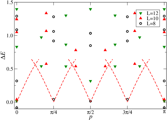
The low energy excitations are gapless with linear dispersion near the Fermi points at $k_{F}=0,\pi$, see Fig. 5.

Refer to caption
Figure 5: Finite size spectrum of the BMW model at $\theta=\eta$ for $\mathcal{L}=12$: energies $\Delta E=E(\mathcal{L})-E_{\theta=\eta}^{(0)}$ are shown in units of $2\pi v_{F}/\mathcal{L}$. The dashed line indicates the dispersion (35) of low energy excitations in the thermodynamic limit.

To calculate the corresponding Fermi velocity, we observe that the contribution of each individual string to the energy and momentum can be expressed in terms of their root density in the thermodynamic limit

$\displaystyle\epsilon(u)$ $\displaystyle=\frac{\pi\cos(\frac{\pi}{4}+\eta)}{8\cos(\frac{\pi}{10})}\rho(u)\,,$ (35)
$\displaystyle p(u)$ $\displaystyle=\pi\int^{u}\mathrm{d}v\,\rho(v)\,.$

Eliminating the rapidity $u$ we obtain the dispersion relation $\epsilon(p)$ of the elementary excitations in the system and the Fermi velocity is obtained to be

$$v_{F}=\frac{5\cos(\frac{\pi}{4}+\eta)}{4\cos(\frac{\pi}{10})}\,\,\approx\,\,1.021807736\,.$$

IV.2.2 Thermodynamic limit of the BMW model at $\theta=\eta+\pi$

For $\theta=\eta+\pi$ the ground state in the thermodynamic limit consists of only $+$- and $-$-strings appearing in a ratio of five to three. For finite size systems we find that the ground state is only realized when $\mathcal{L}$ is a multiple of 8. As we have two different types of string configurations appearing we have two root densities defined by coupled integral equations

$\displaystyle\rho_{+}(u)$ $\displaystyle=-A^{\prime}(u;\frac{1}{20})+\int_{-\infty}^{\infty}\mathrm{d}v\,\rho_{+}(v)A^{\prime}(u-v;\frac{2}{5})+\int_{-\infty}^{\infty}\mathrm{d}v\,\rho_{-}(v)A^{\prime}(u-v;\frac{9}{10})\,,$
$\displaystyle\rho_{-}(u)$ $\displaystyle=-A^{\prime}(u;\frac{11}{20})+\int_{-\infty}^{\infty}\mathrm{d}v\,\rho_{+}(v)A^{\prime}(u-v;\frac{9}{10})+\int_{-\infty}^{\infty}\mathrm{d}v\,\rho_{-}(v)A^{\prime}(u-v;\frac{2}{5})\,.$

Again, these integral equations are straightforward to solve by Fourier transform giving

$$\rho_{\pm}(u)=\frac{5}{2\pi}\left(\frac{\pm 1+\sqrt{2}\cos(\frac{3\pi}{8})\cosh(\frac{5}{2}u)+\sqrt{2}\cos(\frac{\pi}{8})\cosh(\frac{15}{2}u)}{\cosh(10u)}\right)\,.$$

As was the case with the previous critical integrable point, the dressed energies of $\pm$-strings are scalar multiples of the corresponding root densities,

$$\epsilon_{\pm}(u)=\frac{\pi\cos(\frac{\pi}{4}+\eta)}{8\cos(\frac{\pi}{10})}\rho_{\pm}(u)\,.$$

Again the system has massless excitations with linear dispersion near its Fermi points, which in this case are at multiples of $\frac{\pi}{4}$, see Fig. 6.

Refer to caption
Figure 6: Finite size spectrum of the BMW model at $\theta=\eta+\pi$: energies $\Delta E=E(\mathcal{L})-E_{\theta=\eta+\pi}^{(0)}$ are shown in units of $2\pi v_{F}/\mathcal{L}$ for $\mathcal{L}=8$, $10$, $12$. The dashed line indicates the dispersion of low energy excitations in the thermodynamic limit (scaled for $\mathcal{L}=10$), see also Ref. Finch et al., 2014.

The ground state energy density and Fermi velocity are

$\displaystyle\frac{E^{(0)}_{\theta=\eta+\pi}}{\mathcal{L}}$ $\displaystyle=\frac{1}{2}\cos\eta\left\{1+\frac{1}{4i\cos(\frac{\pi}{10})}\int_{-\infty}^{\infty}\mathrm{d}u\,\left[\rho_{+}(u)\frac{\cosh(u+\frac{i\pi}{20})}{\sinh(u+\frac{i\pi}{20})}+\rho_{-}(u)\frac{\cosh(u+\frac{11i\pi}{20})}{\sinh(u+\frac{11i\pi}{20})}\right]\right\}\,$
$\displaystyle\approx\,-0.7578846235\,,$
$\displaystyle v_{F}$ $\displaystyle=\frac{5}{128\sqrt{\frac{11}{8}+\frac{\sqrt{5}}{8}}\left(\cos(\frac{\pi}{40})\right)^{4}-128\sqrt{\frac{11}{8}+\frac{\sqrt{5}}{8}}\left(\cos(\frac{\pi}{40})\right)^{2}+16\sqrt{\frac{11}{8}+\frac{\sqrt{5}}{8}}}\,$
 $\displaystyle\approx\,0.2554519349\,.$

V Finite size spectra and conformal field theory

The models at $\theta=\eta,\pi+\eta$ derived from the BMW transfer matrices constructed above are critical and therefore expected to be described by conformal field theories (CFTs). As a consequence of conformal invariance in the continuum limit the scaling behavior of the ground state energy is predicted to be Blöte et al. (1986); Affleck (1986)

$$E^{(0)}(\mathcal{L})=\epsilon_{\infty}\mathcal{L}-\frac{\pi v_{F}}{6\mathcal{L}}\,c+o(\mathcal{L}^{-1}),$$ (36)

where $c$ is the central charge of the underlying Virasoro algebra and $v_{F}$ is the Fermi velocity. The primary fields present in the critical model determine the finite size energies and momenta of the excited states ($P^{(0)}$ being the momentum at one of the Fermi points)

$$E(\mathcal{L})-E^{(0)}(\mathcal{L})=\frac{2\pi v_{F}}{\mathcal{L}}\left(X+n+\bar{n}\right)\,,\quad P(\mathcal{L})-P^{(0)}=\frac{2\pi}{\mathcal{L}}\left(s+n-\bar{n}\right)+\mathrm{const.}\,.$$ (37)

This allows us to determine the scaling dimensions $X=h+\bar{h}$ and conformal spins $s=h-\bar{h}$ of the primary fields present in the CFT from the spectrum of the lattice model ($n$, $\bar{n}$ are non-negative integers). Solving the Bethe equations numerically for root configurations corresponding to a particular excitation for various lattice sizes we obtain a sequence of finite size estimations for the scaling dimensions

$$X^{\mathrm{num}}_{\theta}(\mathcal{L})=\frac{\mathcal{L}}{2\pi v_{F}}\left(E(\mathcal{L})-E^{(0)}(\mathcal{L})\right)\,.$$ (38)

This sequence is then extrapolated to obtain a numerical approximation $X_{\theta}^{\mathrm{ext}}$ to the scaling dimension, which is subsequently identified with a pair $(h,\bar{h})$ of conformal weights. Similarly, the central charge can be computed by finite size scaling analysis of the ground state energy based on (36).

V.1 The BMW model at $\theta=\eta$

Solving the Bethe equations for the ground state configuration of $4$-strings in systems with even $\mathcal{L}$ we find the scaling of the ground state energy

$$E^{(0)}(\mathcal{L})=E^{(0)}_{\theta=\eta}-0.6114471233\,\mathcal{L}^{-1}+o(\mathcal{L}^{-1})\,.$$

This implies that the central charge is $c=1.14285(1)$, predicted to be actually $\frac{8}{7}$ in agreement with the ferromagnetic $Z_{5}$ Fateev-Zamolodchikov model. This central charge appears in several rational CFTs from the minimal series of Casimir-type $\mathcal{W}$-algebras, see Appendix B. Restricting ourselves to unitary ones these are

$\displaystyle A_{4}:$ $\displaystyle\mathcal{W}(2,3,4,5)$ $\displaystyle c_{A_{4}}(6,7)\,,$
$\displaystyle B_{2}:$ $\displaystyle\mathcal{W}(2,4)$ $\displaystyle c_{B_{2}}(5,7)\,,$
$\displaystyle C_{2}:$ $\displaystyle\mathcal{W}(2,4)$ $\displaystyle c_{C_{2}}(5,7)\,.$

Note that $A_{4}={SL}(5)$ with real form ${SU}(5)$ contains $B_{2}={SO}(5)$ and $C_{2}={Sp}(4)$ as a subalgebra. Since $B_{2}\cong C_{2}$ we only consider the former.333We also note that the microscopic description of the model in terms of ${SO}(5)$ anyons does not go together with the symplectic structure of $C_{2}$.

To identify the low energy effective theory of this anyon model we extend our analysis to the scaling dimensions obtained from the finite size spectrum of excited states, see Table 3.

Sector(s) $X^{\mathrm{ext}}$ $X^{\mathrm{CFT}}$ $s$ $(h,\bar{h})$ $N_{4s}$ $N_{0}$
$\psi_{1}\oplus\psi_{6}$ 0.00000(1) 0 0.00 $(0,0)$ $\frac{\mathcal{L}}{2}$ 0
$\psi_{3}\oplus\psi_{4}$ 0.07144(1) $\frac{1}{14}$ 0.00 $(\frac{1}{28},\frac{1}{28})$ $\frac{\mathcal{L}}{2}$ 0
$\psi_{2}$ 0.117(1) $\frac{4}{35}$ 0.00 $(\frac{2}{35},\frac{2}{35})$ $\frac{\mathcal{L}}{2}-1$ 2
$\psi_{5}$ 0.17146(1) $\frac{6}{35}$ 0.00 $(\frac{3}{35},\frac{3}{35})$ $\frac{\mathcal{L}}{2}-1$ 0
$\psi_{3}\oplus\psi_{4}$ 0.2147(2) $\frac{3}{14}$ 0.00 $(\frac{3}{28},\frac{3}{28})$ $\frac{\mathcal{L}}{2}-1$ 4
$\psi_{3}\oplus\psi_{4}$ 0.50001(1) $\frac{1}{2}$ 0.00 $(\frac{1}{4},\frac{1}{4})$ $\frac{\mathcal{L}}{2}-1$ 4
$\psi_{1}\oplus\psi_{6}$ 0.579(2) $\frac{4}{7}$ 0.00 $(\frac{2}{7},\frac{2}{7})$ $\frac{\mathcal{L}}{2}-2$ 8
$\psi_{3}\oplus\psi_{4}$ 1.068(2) $1\frac{1}{14}$ 1.00 - $\frac{\mathcal{L}}{2}-1$ 4
$\psi_{3}\oplus\psi_{4}$ 1.07148(1) $1\frac{1}{14}$ 1.00 - $\frac{\mathcal{L}}{2}-1$ 4
$\psi_{3}\oplus\psi_{4}$ 1.07211(1) $\frac{15}{14}$ 0.00 $(\frac{15}{28},\frac{15}{28})$ $\frac{\mathcal{L}}{2}-2$ 8
Table 3: Scaling dimensions obtained from the finite size spectrum of the BMW model $\mathcal{H}_{\theta=\eta}$ with even $\mathcal{L}$ corresponding to a $c=\frac{8}{7}$ model. The scaling dimensions, $X^{\mathrm{ext}}$, and the corresponding error estimates are obtained by extrapolation of the numerical finite size energies (38) for $\mathcal{L}$ up to 300. $X^{\mathrm{CFT}}$ is the scaling dimension from the conjectured CFT, $s$ is the conformal spin of the level as obtained from the finite size data. For primary fields we also display the corresponding pair of conformal weights ($h,\bar{h})$. $N_{4s}$ and $N_{0}$ denote the number of 4-strings and other Bethe roots, respectively, appearing in the Bethe root configuration.

Clearly our data rule out the $Z_{5}$ parafermions since the conformal weights observed in the sector $\psi_{3}\oplus\psi_{4}$, e.g. $\frac{1}{28}$, $\frac{3}{28}$ and $\frac{15}{28}$, are not present in the spectrum (47) for $k=5$. On the other hand the finite size data are compatible with the $\mathcal{W}B_{2}(5,7)$ minimal model (67): the conformal weights up to $h=2/7$ are complete, the first one missing is $h=17/35$. This is not surprising as the numerical analysis gets more demanding for higher values of the conformal weight. Therefore, we conclude that if the continuum limit of this BMW model is described by a rational conformal field theory, it presumably is the $(5,7)$ minimal model of the $\mathcal{W}{B}_{2}$ series.

V.2 The BMW model at $\theta=\pi+\eta$

Using the finite size data for the ground state we find the scaling behavior,

$$E^{(0)}(\mathcal{L})=E^{(0)}_{\theta=\eta+\pi}-0.1337534147\,\mathcal{L}^{-1}+o(\mathcal{L}^{-1})$$

from which we can calculate the central charge $c=0.99999(1)$ in agreement with $c=1$ for the anti-ferromagnetic $Z_{5}$ FZ model. Again there are several rational CFTs in the minimal series of Casimir-type $\mathcal{W}$-algebras with the same central charge:

$\displaystyle A_{3}:$ $\displaystyle\mathcal{W}(2,3,4)$ $\displaystyle c_{A_{3}}(5,6)\,,$
$\displaystyle B_{n}:$ $\displaystyle\mathcal{W}(2,4,\ldots,2n)$ $\displaystyle c_{B_{n}}(n,n+1)\ \ \textrm{and}\ \ c_{B_{n}}(2n-1,2n)\,,$
$\displaystyle\mathcal{W}(2,4,\ldots,2n,{\textstyle\frac{1}{2}}(2n+1))$ $\displaystyle c_{\mathcal{B}_{0,n}}(2n,2n+1)\,,$
$\displaystyle C_{n}:$ $\displaystyle\mathcal{W}(2,4,\ldots,2n)$ $\displaystyle c_{C_{n}}(n,2n-1)\ \ \textrm{and}\ \ c_{C_{n}}(n+1,2n)\,,$
$\displaystyle D_{n}:$ $\displaystyle\mathcal{W}(2,4,\ldots,2n-2,n)$ $\displaystyle c_{D_{n}}(2n-1,2n)\,.$

The unitary models ones among these are $\mathcal{W}A_{3}(5,6)$, the $C_{3}$-model $\mathcal{W}C_{3}(3,5)$, and the generic series of minimal models for $\mathcal{B}_{0,\ell}=OSp(1,2\ell)$ and $D_{\ell}={SO}({2\ell})$, i.e. $\mathcal{WB}_{0,\ell}(2\ell,2\ell+1)$ and $\mathcal{W}D_{\ell}(2\ell-1,2\ell)$. Keeping in mind the ${SO}(5)$ anyon structure of the underlying lattice model, the $C_{3}$-model with its symplectic ${Sp}(6)$ symmetry appears to be an unlikely candidate for the low energy effective theory.

To identify which $c=1$ CFT is realized we can look at the finite size properties of low-lying excitations presented in Tables 47.

Sector(s) $P^{(0)}$ $X^{\mathrm{ext}}$ $X^{\mathrm{CFT}}$ $s$ $(h,\bar{h})$ $N_{+}$ $N_{-}$ $N_{0}$
$\psi_{1}\oplus\psi_{6}$ 00 0.00000(1) 0 0.00 $(0,0)$ $\frac{5\mathcal{L}}{4}$ $\frac{3\mathcal{L}}{4}$ 0
$\psi_{2}$ $\frac{\pi}{2}$ 0.10000(1) $\frac{1}{10}$ 0.00 $(\frac{1}{20},\frac{1}{20})$ $\frac{5\mathcal{L}}{4}-1$ $\frac{3\mathcal{L}}{4}-1$ 0
$\psi_{3}\oplus\psi_{4}$ $\frac{\pi}{4}$,$\frac{3\pi}{4}$ 0.12500(1) $\frac{1}{8}$ 0.00 $(\frac{1}{16},\frac{1}{16})$ $\frac{5\mathcal{L}}{4}$ $\frac{3\mathcal{L}}{4}$ 0
$\psi_{5}$ 00 0.40000(1) $\frac{2}{5}$ 0.00 $(\frac{1}{5},\frac{1}{5})$ $\frac{5\mathcal{L}}{4}-2$ $\frac{3\mathcal{L}}{4}-2$ 0
$\psi_{5}$ $\frac{\pi}{2}$ 0.90000(1) $\frac{9}{10}$ 0.00 $(\frac{9}{20},\frac{9}{20})$ $\frac{5\mathcal{L}}{4}-3$ $\frac{3\mathcal{L}}{4}-1$ 0
$\psi_{2}$ $\frac{\pi}{2}$ 1.10000(1) $1\frac{1}{10}$ 1.00 - $\frac{5\mathcal{L}}{4}-2$ $\frac{3\mathcal{L}}{4}-2$ 2
$\psi_{2}$ $\frac{\pi}{2}$ 1.10000(1) $1\frac{1}{10}$ $-1.00$ -
$\psi_{3}\oplus\psi_{4}$ ${\frac{\pi}{4}}$ 1.12471(8) $1\frac{1}{8}$ 1.00 - $\frac{5\mathcal{L}}{4}-2$ $\frac{3\mathcal{L}}{4}-2$ 4
$\psi_{3}\oplus\psi_{4}$ ${\frac{3\pi}{4}}$ 1.12471(8) $1\frac{1}{8}$ $-1.00$ -
Table 4: Scaling dimensions appearing in the spectrum of $\mathcal{H}_{\theta=\eta+\pi}$ for $\mathcal{L}\mod 8=0$. $P^{(0)}$ lists the Fermi points near which the state is observed in the finite size spectrum. $X^{\mathrm{ext}}$ is prediction for the scaling dimension obtained by extrapolation of the finite size data. $X^{\mathrm{CFT}}$ are the conjectured values for the scaling dimension and $s$ the conformal spins, as obtained from the finite size data. For primary fields we also display the corresponding pair of conformal weights $(h,\bar{h})$. The quantities $N_{+}$, $N_{-}$ and $N_{0}$ correspond respectively to the number of $+$-strings, $-$-strings and other Bethe roots in the Bethe root configuration. Note that among the states with scaling dimension $X=1\frac{1}{8}$ we have only identified the $(1,0)$ and $(0,1)$ descendents of the primaries $(h,\bar{h})=(\frac{1}{16},\frac{1}{16})$ at the Fermi points $\frac{\pi}{4}$ and $\frac{3\pi}{4}$, respectively. For the other two descendents as well as the primary fields with $(\frac{9}{16},\frac{9}{16})$ (with momenta $P^{(0)}=\frac{\pi}{4}$, $\frac{3\pi}{4}$) we have not identified the corresponding root configuration.
Sector(s) $P^{(0)}$ $X^{\mathrm{ext}}$ $X^{\mathrm{CFT}}$ $s$ $(h,\bar{h})$ $N_{+}$ $N_{-}$ $N_{0}$
$\psi_{3}\oplus\psi_{4}$ 0 0.12500(1) $\frac{1}{8}$ 0.00 $(\frac{1}{16},\frac{1}{16})$ $\frac{5(\mathcal{L}-2)}{4}+2$ $\frac{3(\mathcal{L}-2)}{4}2$ 0
$\psi_{3}\oplus\psi_{4}$ $\frac{\pi}{2}$ 0.62500(1) $\frac{5}{8}$ $0.50$ $(\frac{9}{16},\frac{1}{16})$ $\frac{5(\mathcal{L}-2)}{4}+2$ $\frac{3(\mathcal{L}-2)}{4}+0$ 2
$\psi_{3}\oplus\psi_{4}$ $\frac{\pi}{2}$ 0.62500(1) $\frac{5}{8}$ $-0.50$ $(\frac{1}{16},\frac{9}{16})$
$\psi_{5}$ $\frac{3\pi}{4}$ 0.65000(1) $\frac{13}{20}$ $0.25$ $(\frac{9}{20},\frac{1}{5})$ $\frac{5(\mathcal{L}-2)}{4}$ $\frac{3(\mathcal{L}-2)}{4}$ 0
$\psi_{5}$ $\frac{\pi}{4}$ 0.65000(1) $\frac{13}{20}$ $-0.25$ $(\frac{1}{5},\frac{9}{20})$
$\psi_{2}$ $\frac{\pi}{4}$ 0.85000(1) $\frac{17}{20}$ $0.75$ $(\frac{4}{5},\frac{1}{20})$ $\frac{5(\mathcal{L}-2)}{4}$ $\frac{3(\mathcal{L}-2)}{4}$ 2
$\psi_{2}$ $\frac{3\pi}{4}$ 0.85000(1) $\frac{17}{20}$ $-0.75$ $(\frac{1}{20},\frac{4}{5})$
$\psi_{3}\oplus\psi_{4}$ 0 1.12500(1) $\frac{9}{8}$ 0.00 $(\frac{9}{16},\frac{9}{16})$ $\frac{5(\mathcal{L}-2)}{4}$ $\frac{3(\mathcal{L}-2)}{4}$ 4
$\psi_{3}\oplus\psi_{4}$ 0 1.12505(6) $1\frac{1}{8}$ 1.00 - $\frac{5(\mathcal{L}-2)}{4}$ $\frac{3(\mathcal{L}-2)}{4}$ 4
$\psi_{3}\oplus\psi_{4}$ 0 1.12505(6) $1\frac{1}{8}$ $-1.00$ -
Table 5: Same as Table 4 but for $\mathcal{L}\mod 8=2$.
Sector(s) $P^{(0)}$ $X^{\mathrm{ext}}$ $X^{\mathrm{CFT}}$ $s$ $(h,\bar{h})$ $N_{+}$ $N_{-}$ $N_{0}$
$\psi_{2}$ 0 0.10000(1) $\frac{1}{10}$ 0.00 $(\frac{1}{20},\frac{1}{20})$ $\frac{5\mathcal{L}}{4}-1$ $\frac{3\mathcal{L}}{4}-1$ 0
$\psi_{5}$ $\frac{\pi}{2}$ 0.40000(1) $\frac{2}{5}$ 0.00 $(\frac{1}{5},\frac{1}{5})$ $\frac{5\mathcal{L}}{4}-2$ $\frac{3\mathcal{L}}{4}-2$ 0
$\psi_{3}\oplus\psi_{4}$ $\frac{3\pi}{4}$ 0.62500(1) $\frac{5}{8}$ $0.50$ $(\frac{9}{16},\frac{1}{16})$ $\frac{5L}{4}-1$ $\frac{3\mathcal{L}}{4}-1$ 2
$\psi_{3}\oplus\psi_{4}$ $\frac{\pi}{4}$ 0.62500(1) $\frac{5}{8}$ $-0.50$ $(\frac{1}{16},\frac{9}{16})$
$\psi_{3}\oplus\psi_{4}$ $\frac{\pi}{4}$ 0.62500(1) $\frac{5}{8}$ $0.50$ $(\frac{9}{16},\frac{1}{16})$ $\frac{5L}{4}-1$ $\frac{3\mathcal{L}}{4}-1$ 2
$\psi_{3}\oplus\psi_{4}$ $\frac{3\pi}{4}$ 0.62500(1) $\frac{5}{8}$ $-0.50$ $(\frac{1}{16},\frac{9}{16})$
$\psi_{5}$ 0 0.90000(1) $\frac{9}{10}$ 0.00 $(\frac{9}{20},\frac{9}{20})$ $\frac{5\mathcal{L}}{4}-3$ $\frac{3\mathcal{L}}{4}-1$ 0
$\psi_{1}\oplus\psi_{6}$ $\frac{\pi}{2}$ 1.00000(1) 1 $1.00$ $(1,0)$ $\frac{5\mathcal{L}}{4}-1$ $\frac{3\mathcal{L}}{4}-1$ 2
$\psi_{1}\oplus\psi_{6}$ $\frac{\pi}{2}$ 1.00000(1) 1 $-1.00$ $(0,1)$
$\psi_{2}$ 0 1.10000(1) $1\frac{1}{10}$ $1.00$ - $\frac{5\mathcal{L}}{4}-2$ $\frac{3\mathcal{L}}{4}-2$ 2
$\psi_{2}$ 0 1.10000(1) $1\frac{1}{10}$ $-1.00$ -
Table 6: Same as Table 4 but for $\mathcal{L}\mod 8=4$.
Sector(s) $P^{(0)}$ $X^{\mathrm{ext}}$ $X^{\mathrm{CFT}}$ $s$ $(h,\bar{h})$ $N_{+}$ $N_{-}$ $N_{0}$
$\psi_{3}\oplus\psi_{4}$ 0 0.12500(1) $\frac{1}{8}$ 0.00 $(\frac{1}{16},\frac{1}{16})$ $\frac{5(\mathcal{L}-2)}{4}+3$ $\frac{3(\mathcal{L}-2)}{4}+1$ 0
$\psi_{3}\oplus\psi_{4}$ $\frac{\pi}{2}$ 0.62500(1) $\frac{5}{8}$ $0.50$ $(\frac{9}{16},\frac{1}{16})$ $\frac{5(\mathcal{L}-2)}{4}+1$ $\frac{3(\mathcal{L}-2)}{4}+1$ 2
$\psi_{3}\oplus\psi_{4}$ $\frac{\pi}{2}$ 0.62500(1) $\frac{5}{8}$ $-0.50$ $(\frac{1}{16},\frac{9}{16})$
$\psi_{5}$ $\frac{\pi}{4}$ 0.65000(1) $\frac{13}{20}$ $0.25$ $(\frac{9}{20},\frac{1}{5})$ $\frac{5(\mathcal{L}-2)}{4}$ $\frac{3(\mathcal{L}-2)}{4}$ 0
$\psi_{5}$ $\frac{3\pi}{4}$ 0.65000(1) $\frac{13}{20}$ $-0.25$ $(\frac{1}{5},\frac{9}{20})$
$\psi_{2}$ $\frac{3\pi}{4}$ 0.85000(1) $\frac{17}{20}$ $0.75$ $(\frac{4}{5},\frac{1}{20})$ $\frac{5(\mathcal{L}-2)}{4}$ $\frac{3(\mathcal{L}-2)}{4}$ 2
$\psi_{2}$ $\frac{\pi}{4}$ 0.85000(1) $\frac{17}{20}$ $-0.75$ $(\frac{1}{20},\frac{4}{5})$
$\psi_{3}\oplus\psi_{4}$ 0 1.1248(1) $1\frac{1}{8}$ 1.00 - $\frac{5(\mathcal{L}-2)}{4}+1$ $\frac{3(\mathcal{L}-2)}{4}-1$ 4
$\psi_{3}\oplus\psi_{4}$ 0 1.1248(1) $1\frac{1}{8}$ $-1.00$ -
Table 7: Same as Table 4 but for $\mathcal{L}\mod 8=6$.

Clearly, the observed spectrum contains conformal weights not present in the ${Z}_{4}$ parafermion theory, thereby excluding the $A_{3}$-model. Furthermore, we can rule out the $\mathcal{W}{C}_{3}(4,6)$ model: even without explicit computation of the spectrum we just know from the general formula (45) for the conformal weights, that their denominators are of the form $2pq$. Therefore, to yield the denominators $5$ and $20$ observed numerically in the anyon model $2pq$ has to be divisible by $5$.

Among the remaining rational CFTs the smallest ones respecting the five-fold discrete symmetry of the BMW model are the $\mathcal{WB}_{0,2}(4,5)$ model and the $\mathcal{W}{D}_{5}(9,10)$ model. Comparing their spectra (84) and (150) with the numerical data we find that the former does not accommodate all observed weights while all weights of the $(9,10)$ model of the $\mathcal{W}{D}_{5}$ minimal series

$$\left\{0,1,\frac{5}{4},\frac{1}{20},\frac{4}{5},\frac{9}{20},\frac{1}{5},\frac{1}{16},\frac{9}{16}\right\}\,$$ (39)

with $h\leq 1$ have been identified.

A peculiar feature of the low energy spectrum observed numerically is the identification of levels corresponding to operators with non-integer spin $s$, see Tables 57. For the sectors $\psi_{2}$ and $\psi_{5}$, where the total momentum is not determined uniquely in terms of the Bethe roots, see Eq. (34) one can use this fact to determine the Fermi point $P^{(0)}$ at which these levels occur: for example, the levels $(h,\bar{h})\in\{(\frac{1}{5},\frac{9}{20}),(\frac{4}{5},\frac{1}{20})\}$ observed for $\mathcal{L}\mod 4=2$ can only appear at $P^{(0)}=\frac{\pi}{4}$. Changing the length of the system to $\mathcal{L}\mod 4=6$ they are observed at $P^{(0)}=\frac{3\pi}{4}$, indicating that they have to appear with a multiplicity of two in the full partition function.

To provide additional evidence for our proposal that the anyon model is a lattice regularization of a $\mathcal{W}{D}_{5}(9,10)$ rational CFT the modular invariant partition function of the model has to be expressed in terms of the Virasoro characters of the relevant representations of the $\mathcal{W}$-algebra. All representations corresponding to the conformal weights (39) have multiplicity one, except $h=5/4$, $1/16$ and $9/16$, which have trivial multiplicities two. This means that our theory should possess nine independent characters.

From the known embedding structure of Virasoro modules, we know that for a CFT with central charge $c=1$ there is just one null state at level one in the Virasoro vacuum representation, $h=0$. Furthermore, the symmetry generators in the chiral symmetry algebra $\mathcal{W}{D}_{5}$ have dimension $d>3$. Therefore, additional states beyond pure Virasoro descendents can only appear at level four or above. This also implies that any additional null states cannot occur below level eight. The reason is that the Virasoro module generated by $W^{(4)}_{-4}|0\rangle$ has just one Virasoro null state, namely at level five, i.e. at level nine with respect to $|0\rangle$. Furthermore, the lowest possible $\mathcal{W}$-algebra null state could be a linear combination containing $W^{(4)}_{-4}W^{(4)}_{-4}|0\rangle$ at level eight with respect to $|0\rangle$. Analogous statements hold for the Virasoro submodule generated by $W^{(5)}_{-5}|0\rangle$. Therefore, we obtain

$$\chi_{h=0}(q)=\frac{1}{\eta(q)}(1-q+q^{4}+q^{5}\ldots)\,,$$

where $\eta(q)=q^{1/24}\prod_{n=1}^{\infty}(1-q^{n})$ is the Dedekind eta-function.

This insight, together with similar considerations for the other representations, is sufficient to set up a differential equation from which the characters of the rational CFT can be computed to arbitrary powers without additional prior knowledge of the detailed structure of the representations: the modular differential equation encodes the fact that the characters of the nine inequivalent irreps of the CFT form a nine-dimensional representation of the modular group in terms of modular functions with asymptotic behavior fixed by the numbers $h_{i}-\frac{c}{24}$ Mathur et al. (1988). Assuming that all characters can be written as modular forms of weight $1/2$ divided by the Dedekind eta-function we find

$\displaystyle\chi_{0}(q)$ $\displaystyle=\frac{1}{2\eta(q)}\big{(}\Theta_{0,5}(q)+\Theta_{0,4}(q)-\Theta_{4,4}(q)\big{)}\,,$ (40)
$\displaystyle\chi_{1}(q)$ $\displaystyle=\frac{1}{2\eta(q)}\big{(}\Theta_{0,5}(q)-\Theta_{0,4}(q)+\Theta_{4,4}(q)\big{)}\,,$
$\displaystyle\chi_{5/4}(q)$ $\displaystyle=\frac{1}{\eta(q)}\,\Theta_{5,5}(q)\,,$
$\displaystyle\chi_{1/20}(q)$ $\displaystyle=\frac{1}{\eta(q)}\,\Theta_{1,5}(q)\,,\qquad\chi_{4/5}(q)=\frac{1}{\eta(q)}\,\Theta_{4,5}(q)\,,$
$\displaystyle\chi_{9/20}(q)$ $\displaystyle=\frac{1}{\eta(q)}\,\Theta_{3,5}(q)\,,\qquad\chi_{1/5}(q)=\frac{1}{\eta(q)}\,\Theta_{2,5}(q)\,,$
$\displaystyle\chi_{1/16}(q)$ $\displaystyle=\frac{2}{\eta(q)}\,\Theta_{1,4}(q)\,,\qquad\chi_{9/16}(q)=\frac{2}{\eta(q)}\,\Theta_{3,4}(q)\,.$

Here we have used the Jacobi-Riemann Theta-functions

$$\Theta_{\lambda,k}(q)=\sum_{n\in\mathbb{Z}}q^{\frac{(2kn+\lambda)^{2}}{4k}}\,.$$

Note that we have introduced an explicit factor of two in the definition of $\chi_{1/16}(q)$ and $\chi_{9/16}(q)$. In fact, these characters as well as $\chi_{5/4}(q)=2\,q^{-1/24+5/4}\left(1+q+2q^{2}+3q^{3}+5q^{4}+\ldots\right)$ should be read as $\chi_{h}(q)=\chi_{h}^{+}(q)+\chi_{h}^{-}(q)$ being the sum of two identical characters for the two equivalent representations appearing in the Kac-table for $h\in\{\frac{5}{4},\frac{1}{16},\frac{9}{16}\}$, see (150). For the present discussion of the conformal spectrum this is sufficient. In Appendix C, where we compute the fusion rules for the $\mathcal{W}D_{5}((9,10)$ rational CFT, these representations have to be disentangled in a consistent way.

Given (40) the modular $\mathcal{S}$-matrix is easily computed, for the result see Appendix C. Modular invariance of the partition function of the model, expressed as $Z=\sum_{ij}\chi_{i}M_{ij}\bar{\chi}_{j}$ in terms of the characters (40), translates into the condition $M=\mathcal{S}^{\dagger}M\mathcal{S}$ for the matrix $M$ of multiplicities.444Strictly speaking, we have invariance under a subgroup of the modular group only: while the partition function is invariant under the action of $\mathcal{S}:\tau\to-1/\tau$, the presence of fields with quarter spin implies that this is true only for quadruples of the modular transformation $\mathcal{T}:\tau\to\tau+1$. With the $\mathcal{S}$-matrix (151) at hand this condition can be solved and we find

$\displaystyle M_{ij}(n,m,p,q)=$ (41)
$\displaystyle\left(\begin{array}[]{ccccccccc}n&n-q&\frac{1}{2}p&&&&&&\\ n-q&n&\frac{1}{2}p&&&&&&\\ \frac{1}{2}p&\frac{1}{2}p&n-p-\frac{1}{2}q&&&&&&\\ &&&2(n-p)-q&p&&&&\\ &&&p&2n-q&&&&\\ &&&&&2(n-p)-q&p&\\ &&&&&p&2n-q&&\\ &&&&&&&\frac{1}{2}m&\frac{1}{2}(q-m)\\ &&&&&&&\frac{1}{2}(q-m)&\frac{1}{2}m\end{array}\right)\,.$

Rows and columns refer to representations in the order listed in Eq. (39). The four blocks in $M$ match with the decomposition of the spectrum of the lattice model according to topological sectors $\psi_{1}\oplus\psi_{6}$, $\psi_{2}$, $\psi_{5}$, and $\psi_{3}\oplus\psi_{4}$ of the lattice model, see Tables 2 and 47. In Eq. (41) $n,m,p,q$ are non-negative integers such that $M$ has no negative entries and full rank. Half-odd integer entries in (41) are a consequence of our choice for the characters of representations with multiplicity two: for example, from the diagonal partition function, $M_{ij}(1,1,0,1)=\mathrm{diag}(1,1,\frac{1}{2},1,1,1,1,\frac{1}{2},\frac{1}{2})$, one can infer that only either the combination $\chi_{5/4}^{+}\bar{\chi}_{5/4}^{+}+\chi_{5/4}^{-}\bar{\chi}_{5/4}^{-}$ or the combination $\chi_{5/4}^{+}\bar{\chi}_{5/4}^{-}+\chi_{5/4}^{-}\bar{\chi}_{5/4}^{+}$ enters. The same holds for the two representations with $h=1/16$ and $h=9/16$. Of course, linear combinations of arbitrary solutions $M_{ij}(n,m,p,q)$ with non-negative integer coefficients are also possible, but yield nothing new.

From the finite size spectrum of the anyon model we know that $M_{h\bar{h}}=\frac{1}{2}$ for $h,\bar{h}\in\{\frac{1}{16},\frac{9}{16}\}$ which implies $m=1$, $q=2$. Similarly, as discussed above, the quarter spin fields in the symmetry sectors $\psi_{2}$ and $\psi_{5}$ appear twice (with different momentum) in the low energy spectrum, hence $p=2$. As a result the smallest off-diagonal partition function which incorporates all non-diagonal combinations found in our model is $M_{ij}(4,1,2,2)$. This leads to a fourfold degenerate ground state in the model while it is unique in the lattice model with periodic boundary conditions studied here. We expect that the other ground states (corresponding to the degenerate minima of the dispersion at momenta $P^{(0)}=k\frac{\pi}{4}$, $k=1,2,3$) are realized when considering more general (twisted) boundary conditions for the anyon chain.

Finally, we note that in the CFT describing the collective behavior of the BMW model at $\theta=\pi+\eta$ the symmetry of the underlying anyon model appears to be modified. If we understand the ${SO}(5)$ symmetry of the anyons as a discrete one (similar as the cyclic subgroup ${Z}_{5}$ of ${SU}(2)$), however, ${SO}(10)$ could correspond to the dihedral subgroup ${D}_{5}$ of ${SU}(2)$. This is appealing for two reasons: firstly, it would fit with the well known $A$-$D$-$E$ classification of rational conformal field theories with $c=1$ as conformal field theories with extended symmetries given by modding out discrete symmetries of $\widehat{{SU}}(2)$ Ginsparg (1988). Secondly, a similar construction with $D(D_{3})$ anyons also has a $c=1$ point, where it coincides with the ${Z}_{4}$ parafermions Finch and Frahm (2012, 2013). These, however, are $\widehat{{SU}}(4)\cong\widehat{{SO}}(6)$, i.e. $\hat{A}_{3}\cong\hat{D}_{3}$.

VI Discussion

In this paper we have constructed several integrable one-dimensional models of interacting anyons satisfying the fusion rules for $SO(5)_{2}$. For particles carrying topological charge $\psi_{3}$ we have constructed representations of the Birman-Murakami-Wenzl (BMW) algebra (or its Temperley-Lieb (TL) subalgebra) in terms of the local projection operators appearing in the anyon model. Based on these representations we found $R$-matrices solving the Yang-Baxter equation from which commuting transfer matrices have been obtained. The spectrum of these models is parametrized in terms of solutions from Bethe equations which have been derived using the Temperley-Lieb equivalence to the six-vertex model and the fusion hierarchy of transfer matrices, respectively. The topological charges characterizing the spectrum of the anyon chains have been identified with the transfer matrices in the limit of infinite spectral parameter. This allows to classify the spectrum.

By solving the Bethe equations we have identified the ground states and low energy excitations of these models. The TL-models are equivalent to the six-vertex model in its (anti-)ferromagnetic massive phases. The other two integrable models are critical at zero temperature. From the finite size spectrum we have been able to identify the conformal field theories describing their scaling limit. Based on the Bethe ansatz solution we find that these systems are closely related to the $Z_{5}$ Fateev-Zamolodchikov (FZ) or self-dual chiral Potts model. In particular, they have the same Virasoro central charges, i.e. $c=\frac{8}{7}$ and $c=1$, as the ferro- and anti-ferromagnetic $Z_{5}$ FZ model. Careful analysis of the excitation spectrum reveals, however, that the boundary conditions imposed by the conserved topological charges of the anyon model lead to rational conformal field theories with the same central charges but invariant under extensions of the Virasoro algebra, i.e. $\mathcal{W}B_{2}$ and $\mathcal{W}D_{5}$, respectively. The difference between, e.g., the $\mathcal{W}B_{2}(5,7)$ model and $Z_{5}$ parafermions proposed previously for the FZ model, shows up in the presence of additional conformal weights $h\in\{\frac{1}{28},\frac{3}{28},\frac{1}{4},\ldots\}$ in the finite size spectrum which do not appear in the spectrum of the $Z_{5}$ parafermionic theory. For the $\mathcal{W}D_{5}(9,10)$ rational CFT we have computed the characters of the Virasoro representations, $\mathcal{S}$-matrix and fusion rules. Based on the data obtained from the finite size spectrum, an off-diagonal modular invariant partition function has been proposed. This is a first step towards the construction of lattice operators corresponding to the fields appearing in the continuum theory (see e.g. Mong et al. (2014)).

These findings lead us to conjecture that the sequence of $c=1$ theories describing the critical properties of the anti-ferromagnetic $Z_{n}$ FZ models for $n$ odd Albertini (1994) are in fact rational CFTs with $\mathcal{W}D_{n}$ symmetry. For the case $n=3$, corresponding to the 3-state Potts chain, the modular invariant partition function has been computed Kedem and McCoy (1993) leading to the identification of a low energy effective theory with $Z_{4}$ parafermions (see also Ref. Finch and Frahm (2013) for another related anyon chain). This CFT happens to have the same spectrum as the $\mathcal{W}D_{3}$ model. Further support for this conjecture is obtained from the numerical solution of the Bethe equations of the FZ models for $n=7,9$ indicating the presence of $\mathcal{W}D_{n}$ primary fields with conformal weight $h\in\{\frac{k^{2}}{4n}\,|\,k=0\ldots n\}\cup\{\frac{1}{16},\frac{9}{16},1\}$ (note that the exponents $\frac{1}{16}$, $\frac{9}{16}$ appear in the spectrum of the FZ model with $\pi$-twisted boundary conditions).

Finally, let us remark that different anyon chains can be constructed from the $SO(5)_{2}$ fusion rules, Table 1: considering fusion paths (4) for $\psi_{2}$-anyons the neighboring labels are restricted to be adjacent nodes on the graph shown in Figure 7.

$\psi_{1}$ $\psi_{2}$ $\psi_{5}$ $\psi_{6}$ $\psi_{3}$ $\psi_{4}$
Figure 7: The same as Figure 1 except for a chain of $\psi_{2}$ anyons.

In this case the fusion path basis can be decomposed into two decoupled subspaces: the Hilbert space spanned by states with particles $\{\psi_{3},\psi_{4}\}$ is isomorphic to that of a spin-$\frac{1}{2}$ chain. Hence it can be written as a tensor product of local spaces $\mathbb{C}^{2}$ . The complementary set of particles $\{\psi_{1},\psi_{2},\psi_{5},\psi_{6}\}$ forms a fusion category equivalent to categories of irreducible representation of the dihedral group of order 10. Using this insight we can expect that the model is connected to the one-dimensional spin-$\frac{1}{2}$ XXZ model Finch (2013). Indeed we find that the $R$-matrix of the six-vertex model with anisotropy parameter $\gamma$ can be expressed in terms of the local projection operators appearing in this $\psi_{2}$-anyon chain:

$$R(u)=\left(\sinh(\gamma)+\sinh(2u)\right)p^{(1)}+\left(\sinh(\gamma+2u)\right)p^{(5)}+\left(\sinh(\gamma)-\sinh(2u)\right)p^{(6)}\,.$$

The resulting model shares bulk properties with the spin-$\frac{1}{2}$ XXZ chain. As in the case of the $\psi_{3}$-model this does not, however, mean that the excitation spectrum or the operator content will be the same. This is again a consequence of the presence of commuting topological charges modifying the boundary conditions in the anyon model.

Even more models for anyons satisfying a given set of fusion rules can be obtained by using other sets of $F$-moves consistent with the pentagon equation. This may lead to different models similar as in the case of $SU(2)_{3}$ fusion rules leading to both the Fibonacci and the (non-unitary) Yang-Lee anyon chains Feiguin et al. (2007); Ardonne et al. (2011). This question and the possibility of additional integrable models for interacting $SO(5)_{2}$ anyons will be studied in future work.

Acknowledgements.
This work has been supported by the Deutsche Forschungsgemeinschaft under grant no. Fr 737/7.

Appendix A Transfer matrices for the BMW integrable point

To construct the family (19) of transfer matrices $t^{(\ell)}(u)$ we define the functions appearing in the generalized Boltzmann weights (18) to be

$\displaystyle w^{1,3}_{3}(u)$ $\displaystyle=1\,,$
$\displaystyle w^{2,3}_{3}(u)$ $\displaystyle=i\cosh(u)\,,\qquad w^{2,3}_{4}(u)=\sinh(u)\,,$
$\displaystyle w^{3,3}_{1}(u)$ $\displaystyle=\sinh(u+\frac{i\pi}{10})\sinh(u+\frac{3i\pi}{10})\,,$
$\displaystyle w^{3,3}_{2}(u)$ $\displaystyle=\sinh(u-\frac{i\pi}{10})\sinh(u-\frac{3i\pi}{10})\,,$
$\displaystyle w^{3,3}_{5}(u)$ $\displaystyle=\sinh(u+\frac{9i\pi}{10})\sinh(u+\frac{3i\pi}{10})\,,$
$\displaystyle w^{4,3}_{2}(u)$ $\displaystyle=-\sinh(u+\frac{2i\pi}{5})\sinh(u+\frac{i\pi}{5})\,,$
$\displaystyle w^{4,3}_{3}(u)$ $\displaystyle=-\sinh(u+\frac{2i\pi}{5})\sinh(u-\frac{i\pi}{5})\,,$
$\displaystyle w^{4,3}_{6}(u)$ $\displaystyle=\sinh(u-\frac{2i\pi}{5})\sinh(u-\frac{i\pi}{5})\,,$
$\displaystyle w^{5,3}_{3}(u)$ $\displaystyle=\mathrm{e}^{\frac{8i\pi}{10}}\,,\qquad w^{5,3}_{4}(u)=\mathrm{e}^{\frac{3i\pi}{10}}\,,$
$\displaystyle w^{6,3}_{4}(u)$ $\displaystyle=-i\,.$

The additional weights are constructed from (16) as descendents Bazhanov and Stroganov (1990).

Among the resulting transfer matrices $t^{(\ell)}(u)$, the ones for $\ell=1,5,6$ are found to be independent of the spectral parameter $u$. For $t^{(1)}(u)$ and $t^{(6)}(u)$ this follows from $\psi_{1}\otimes\psi_{3}$ and $\psi_{6}\otimes\psi_{3}$ both being isomorphic to simple objects. The absence of a parameter in $t^{(5)}(u)$ is connected to our choice of representation of the BMW algebra. The different representations and their corresponding $R$-matrices lead to different sets of transfer matrices and we find that it is always the case that either $t^{(2)}(u)$ or $t^{(5)}(u)$ is parameter independent.

From the analysis of small systems, $\mathcal{L}\leq 10$, we find that the topological $Y$-operators (5) are obtained as limits of the transfer matrices, i.e.

$\displaystyle t^{(1)}(u)$ $\displaystyle=$ $\displaystyle Y_{1}\,,$
$\displaystyle\lim_{u\rightarrow\pm\infty}\left[2^{\mathcal{L}}\mathrm{e}^{\mp\left(u+\frac{7i\pi}{10}\right)\mathcal{L}}\times t^{(2)}(u)\right]$ $\displaystyle=$ $\displaystyle Y_{2}\,,$
$\displaystyle\lim_{u\rightarrow\pm\infty}\left[4^{\mathcal{L}}\mathrm{e}^{\mp\left(2u+\frac{9i\pi}{10}\right)\mathcal{L}}\times t^{(3)}(u)\right]$ $\displaystyle=$ $\displaystyle Y_{3}\,,$
$\displaystyle\lim_{u\rightarrow\pm\infty}\left[4^{\mathcal{L}}\mathrm{e}^{\mp\left(2u+\frac{2i\pi}{5}\right)\mathcal{L}}\times t^{(4)}(u)\right]$ $\displaystyle=$ $\displaystyle Y_{4}\,,$
$\displaystyle t^{(5)}(u)$ $\displaystyle=$ $\displaystyle Y_{5}\,,$
$\displaystyle t^{(6)}(u)$ $\displaystyle=$ $\displaystyle Y_{6}\,.$

Given the interpretation of both the $t^{(\ell)}(u)$ and the $Y_{\ell}$ as descriptions of certain braiding processes we expect this relation to hold for arbitrary system sizes. Using the fusion procedure Bazhanov and Reshetikhin (1989) for face models we find closed relations for transfer matrices

$\displaystyle t^{(6)}(u)\,t^{(6)}(u)$ $\displaystyle=\mathbf{1}\,,$ (42)
$\displaystyle t^{(6)}(u)\,t^{(3)}(u)$ $\displaystyle=i^{\mathcal{L}}\,t^{(4)}(u+\frac{i\pi}{2})\,,$
$\displaystyle t^{(2)}(u)\,t^{(3)}(u)$ $\displaystyle=\left[\sinh\left(u-\frac{i\pi}{10}\right)\right]^{\mathcal{L}}\,t^{(3)}(u+\frac{2i\pi}{5})+\left[\sinh\left(u\right)\right]^{\mathcal{L}}\,t^{(4)}(u+\frac{i\pi}{10})$
$\displaystyle=\left[\sinh\left(u-\frac{i\pi}{10}\right)\right]^{\mathcal{L}}\,t^{(3)}(u+\frac{2i\pi}{5})+\left[i\sinh\left(u\right)\right]^{\mathcal{L}}\,t^{(6)}(u)\,t^{(3)}(u-\frac{2i\pi}{5})\,.$

Examining Table 1 we see that the relations between transfer matrices mimic the fusions rules of the underlying category.

Appendix B Rational CFTs with extended symmetries

As discussed in the main text the finite size spectrum of a critical one-dimensional lattice model is completely determined by the central charge $c$ of the underlying Virasoro algebra and the spectrum of conformal weights $\{h\}$, i.e. the eigenvalues of the Virasoro zero mode $L_{0}$ on the primary (or Virasoro highest weight) states. Often, however, the Virasoro algebra alone is not sufficient to decompose the state space of the system into a finite set of irreducible highest weight representations. We collect here some general facts about rational CFTs with extended chiral symmetry algebras, mainly taken from Figueroa-O’Farrill (1990); Lukyanov and Fateev (1990); Bouwknegt and Schoutens (1993); Frenkel et al. (1992); Blumenhagen et al. (1995) and the reprint volume Bouwknegt and Schoutens (1995).

B.1 Chiral symmetry algebras

This is true in particular for rational conformal field theories with $c\geq 1$: these theories having a finite number of admissible highest weight representations with respect to its maximally extended chiral symmetry algebra $\mathcal{W}(d_{1}=2,d_{2},\ldots,d_{\ell})$. Here $d_{k}$ denote the conformal scaling dimensions of chiral primary fields $W^{(d_{k})}$ which, together with the energy-momentum tensor $T\equiv W^{(d_{1})}$, generate the chiral symmetry algebra. A highest weight state $\left|h\equiv w^{(1)},w^{(2)},w^{(3)},\ldots w^{(\ell)}\right>$ has then $\ell$ quantum numbers $w^{(k)}$ with respect to the zero modes $W^{(d_{k})}_{0}$, i.e. $W^{(d_{k})}_{0}\left|h,w^{(2)},w^{(3)},\ldots w^{(\ell)}\right>=w^{(k)}\left|h,w^{(2)},w^{(3)},\ldots w^{(\ell)}\right>$. The highest weight representations are closed under fusion and hence give rise to a finite-dimensional representation of the modular group $\mathrm{PSL}(2,\mathbb{Z})$. As all fields in the symmetry algebra must be mutually local, the scaling dimensions are restricted to be integers or half-integers, $2\,d_{k}\in\mathbb{N}$. Therefore, chiral symmetry algebras constitute meromorphic conformal field theories.

A class of chiral symmetry algebras whose representation theory is particularly well understood are $\mathcal{W}$-algebras associated with Lie-algebras $\mathfrak{g}$, where the scaling dimensions $d_{k}$ are related to the exponents of the Lie-algebra $\mathfrak{g}$, i.e. where one has one $W^{(d_{k})}$ field associated to each independent Casimir operator. For a Lie-algebra of rank $\ell$, the $\mathcal{W}$-algebra is generated by $\ell$ such fields, one of those always being the Virasoro field associated to the quadratic Casimir operator. For this class of $\mathcal{W}$-algebras, free field realizations are known and hence the algebras can, in principle, be explicitly constructed Frenkel et al. (1992). For all semi-simple Lie-algebras the corresponding $\mathcal{W}$-algebras are known together with their so-called minimal series of rational theories they admit.

In the following let $\mathfrak{g}$ denote a simple Lie-algebra of rank $\ell$, and $\mathfrak{h}$ a Cartan subalgebra of it. We denote by $d_{\mathfrak{g}}$ the dimension of the Lie-algebra and by $g^{*}$ its dual Coxeter number. Let $\Phi_{+}$ denote the set of positive roots $\alpha$, and $\mathrm{ht}\,\alpha$ the height of the root $\alpha$. The height of a positive root is determined from its unique decomposition $\alpha=\sum_{i=1}^{r}n_{i}\alpha_{i}$ into a linear combination of the simple roots $\alpha_{i}$ with non-negative integers $n_{i}$: $\mathrm{ht}\,\alpha=\sum_{i=1}^{r}n_{i}$. Finally, the maximal root may be denoted by $\rho$. Under affinization of the Lie-algebra to $\hat{\mathfrak{g}}$, we introduce the level $x=2k/|\rho|^{2}$, where $k$ is the central extension of $\hat{\mathfrak{g}}$. Choosing the Killing form as our invariant symmetric bilinear form on $\mathfrak{g}$, one finds that $|\rho|^{2}=1/g^{*}$ and the central charge for $\mathcal{W}_{\hat{\mathfrak{g}}}$ at level $x$ is given by Figueroa-O’Farrill (1990)

$\displaystyle c_{\mathfrak{g}}(x)$ $\displaystyle=\ell-\frac{d_{\mathfrak{g}}g^{*}}{x+g^{*}}-\frac{12}{g^{*}}(x+g^{*})\sum_{\alpha\in\Phi_{+}}(\mathrm{ht}\,\alpha)^{2}+12\sum_{\alpha\in\Phi_{+}}\mathrm{ht}\,\alpha\,.$ (43)

We see that the central charge is entirely expressed in terms of basic properties of the Lie-algebra and the sums of the (squares of the) heights of the positive roots. The former are standard and can be found in every text book on Lie-algebras, the latter can easily be computed from the explicit choice of set of simple roots $\Delta$. In fact, the values of these sums do not depend on the choice of $\Delta$ after all. The data needed to explicitely compute the central charge for a simple Lie algebra are given in Table 8.

$\mathfrak{g}$ $d_{\mathfrak{g}}$ $g^{*}$ $\sum_{\alpha\in\Phi_{+}}\mathrm{ht}\,\alpha$ $\sum_{\alpha\in\Phi_{+}}(\mathrm{ht}\,\alpha)^{2}$
$A_{\ell}$ $\ell(\ell+2)$ $\ell+1$ $\frac{1}{6}\ell(\ell+1)(\ell+2)$ $\frac{1}{12}\ell(\ell+1)^{2}(\ell+2)$
$B_{\ell}$ $\ell(2\ell+1)$ $2\ell-1$ $\frac{1}{6}\ell(\ell+1)(4\ell-1)$ $\frac{1}{6}\ell(\ell+1)(2\ell-1)(2\ell+1)$
$C_{\ell}$ $\ell(2\ell+1)$ $\ell+1$ $\frac{1}{6}\ell(\ell+1)(4\ell-1)$ $\frac{1}{6}\ell(\ell+1)(2\ell-1)(2\ell+1)$
$D_{\ell}$ $\ell(2\ell-1)$ $2(\ell-1)$ $\frac{1}{3}\ell(\ell-1)(2\ell-1)$ $\frac{1}{3}\ell(\ell-1)^{2}(2\ell-1)$
$E_{6}$ $78$ $12$ $156$ $936$
$E_{7}$ $133$ $18$ $399$ $3591$
$E_{8}$ $248$ $30$ $1240$ $18600$
$F_{4}$ $52$ $9$ $110$ $702$
$G_{2}$ $14$ $4$ $16$ $56$
$\mathcal{B}_{0,\ell}$ $\ell(2\ell+1)$ $2\ell-1$ $\frac{1}{6}\ell(2\ell-1)(2\ell+1)$ $\frac{1}{12}\ell(2\ell-1)^{2}(2\ell+1)$
Table 8: Lie algebra data.

B.2 Minimal series of Casimir-type $\mathcal{W}$-algebras

Setting $x+g^{*}=p/q\in\mathbb{Q}$ with $p,q$ coprime positive integers in (43) one obtains the minimal series of a chiral symmetry algebra, i.e. a series of values of the central charge $c_{\mathfrak{g}}(p,q)$, where due to an exceptional high number of null states per Verma module the irreducible representations are as small as possible. For these values of $c$ only finitely many irreducible highest weight representations are needed to build a complete, rational conformal field theory. The corresponding $L_{0}$ eigenvalues of the highest weight states are all known.

In Table 9 we give a list of all the Casimir-type $\mathcal{W}_{\hat{\mathfrak{g}}}$-algebras, explicitly denoting the dimensions $d_{k}$ of their generators.

$\mathfrak{g}$ $\mathcal{W}_{\hat{\mathfrak{g}}}$ $c_{\mathfrak{g}}(p,q)$
$A_{\ell}$ $\mathcal{W}A_{\ell}=\mathcal{W}(2,3,\ldots,d,\ldots,\ell+1)$ $\ell\left(1-(\ell+1)(\ell+2)\frac{(p-q)^{2}}{pq}\right)$
$B_{\ell}$ $\mathcal{W}B_{\ell}=\mathcal{W}(2,4,\ldots,2d,\ldots,2\ell)$ $\ell\left(1+2(\ell+1)(4\ell-1)-(2\ell+1)\Big{(}\frac{(2\ell-1)q}{p}+\frac{2(\ell+1)p}{q}\Big{)}\right)$
$C_{\ell}$ $\mathcal{W}C_{\ell}=\mathcal{W}(2,4,\ldots,2d,\ldots,2\ell)$ $\ell\left(1+2(\ell+1)(4\ell-1)-(2\ell+1)\Big{(}\frac{2(2\ell-1)q}{p}+\frac{(\ell+1)p}{q}\Big{)}\right)$
$D_{\ell}$ $\mathcal{W}D_{\ell}=\mathcal{W}(2,4,\ldots,2d,\ldots,2(\ell-1),\ell)$ $\ell\left(1-(2\ell-1)(2\ell-2)\frac{(p-q)^{2}}{pq}\right)$
$E_{6}$ $\mathcal{W}E_{6}=\mathcal{W}(2,5,6,8,9,12)$ $6\left(1-156\frac{(p-q)^{2}}{pq}\right)$
$E_{7}$ $\mathcal{W}E_{7}=\mathcal{W}(2,6,8,10,12,14,18)$ $7\left(1-342\frac{(p-q)^{2}}{pq}\right)$
$E_{8}$ $\mathcal{W}E_{8}=\mathcal{W}(2,8,12,14,18,20,24,30)$ $8\left(1-930\frac{(p-q)^{2}}{pq}\right)$
$F_{4}$ $\mathcal{W}F_{4}=\mathcal{W}(2,6,8,12)$ $4\left(1+330-117\Big{(}\frac{2p}{q}+\frac{q}{p}\Big{)}\right)$
$G_{2}$ $\mathcal{W}G_{2}=\mathcal{W}(2,6)$ $2\left(1+96-28\Big{(}\frac{3p}{q}+\frac{q}{p}\Big{)}\right)$
$\!\!\mathcal{B}_{0,\ell}$ $\mathcal{WB}_{0,\ell}=\mathcal{W}(2,4,\ldots,2\ell,\frac{1}{2}(2\ell+1))$ $(\ell+\frac{1}{2})\left(1-2\ell(2\ell-1)\frac{(p-q)^{2}}{pq}\right)$
Table 9: Casimir-type $\mathcal{W}$-algebras and their corresponding minimal series.

By definition, the first generator, always of scaling dimension two, is the energy-momentum tensor, all other generators are Virasoro primary fields. Casimir-type $\mathcal{W}$-algebras are purely bosonic algebras, i.e. all generators have integer scaling dimensions. For each of the algebras, we also list the central charges of their corresponding series of minimal models for level $x+g^{*}=p/q\in\mathbb{Q}$.

For non-simply-laced Lie-algebras alternative constructions of extended chiral symmetries are possible if one allows for generators with half-integer spin. In particular Lukyanov and Fateev (1990), one can construct an alternative $\mathcal{W}$-algebra for the $B_{\ell}$ series, i.e. for ${SO}(2\ell+1)$, which contains precisely one fermionic generator. In the literature, these algebras are often denoted $\mathcal{W}_{\hat{B}f}$-algebras, and are given as $\mathcal{W}(2,4,\ldots,2d,\ldots,2\ell,\frac{1}{2}(2\ell+1))$. We will denote them as $\mathcal{WB}_{0}$-algebras in the following. These algebras also admit a minimal series whose members have the central charges

$\displaystyle c_{\mathcal{B}_{0,\ell}}(p,q)$ $\displaystyle=\Big{(}\ell+\frac{1}{2}\Big{)}\left(1-2\ell(2\ell-1)\frac{(p-q)^{2}}{pq}\right)\,.$ (44)

We note that the first member, $\mathcal{W}_{\hat{\mathcal{B}}_{0,1}}=\mathcal{W}(2,\frac{3}{2})$, yields the minimal series of the $N=1$ supersymmetric extension of the Virasoro algebra, when $p$ and $q$ are replaced by half-integers $p/2$ and $q/2$. In general, the $\mathcal{WB}_{0}$-algebras can be realized from the Lie-superalgebras $\mathcal{B}_{0,\ell}={OSp}(1|2\ell)$, which explains our notation. This is the only example of a Lie-superalgebra leading to a true Casimir-type $\mathcal{W}$-algebra. Note that the central charge (44) can formally be obtained from Eq. (43) for $D_{\ell}$ by replacing $\ell\mapsto\ell+\frac{1}{2}$.

B.3 Spectra of Casimir-type $\mathcal{W}$-algebras

In a similar way as the central charges (43) the conformal weights appearing in minimal models of Casimir-type $\mathcal{W}$-algebras are essentially determined by data from the underlying Lie-algebra. Let again $\ell$ denote the rank of a simple Lie-algebra $\mathfrak{g}$.

Highest-weight representations of $\mathfrak{g}$ to weights $\lambda=\sum_{i=1}^{\ell}r_{i}\lambda^{i}$ with $\lambda^{i}$ denoting the fundamental weights, and $r_{i}\in\mathbb{N}$ can be labeled by the positive integers $\mathbf{r}=(r_{1},r_{2},\ldots,r_{\ell})$. The weight lattice has an associated dual lattice, spanned by the fundamental co-roots $\lambda^{*}_{i}$. A co-weight is then given by $\lambda^{*}=\sum_{i=1}^{\ell}s^{i}\lambda^{*}_{i}$ with $s^{i}\in\mathbb{N}$ and labeled by the positive integers $\mathbf{s}=(s^{1},s^{2},\ldots,s^{\ell})$. The conformal weights of a minimal model of a Casimir-type $\mathcal{W}$-algebra $\mathcal{W}_{\hat{\mathfrak{g}}}$ with central charge $c_{\mathfrak{g}}(p,q)$ are given by Lukyanov and Fateev (1990); Blumenhagen et al. (1995)

$\displaystyle h_{\mathbf{r},\mathbf{s}}(p,q)$ $\displaystyle=\frac{q^{2}\,\mathbf{r}\cdot(C^{-1}D)\cdot\mathbf{r}-2pq\,\mathbf{r}\cdot(C^{-1})\cdot\mathbf{s}+p^{2}\,\mathbf{s}\cdot(D^{-1}C^{-1})\cdot\mathbf{s}}{2pq}-\frac{\ell-c_{\mathfrak{g}}(p,q)}{24}\,,$ (45)

where $C$ denotes the Cartan matrix of the simple Lie-algebra $\mathfrak{g}$, and where the weights and co-weights must fulfill the conditions $\sum_{i=1}^{\ell}r_{i}m^{i}\leq p-1$ and $\sum_{i=1}^{\ell}s^{i}m^{*}_{i}\leq q-1$. Here, the $m^{i}$ are the normalized components of the highest root $\psi$ in the directions of the simple roots $\alpha_{i}$, i.e. $\frac{\psi}{\psi^{2}}=\sum_{i=1}^{\ell}m^{i}\frac{\alpha_{i}}{\alpha_{i}^{2}}$ and $m^{*}_{i}=\frac{2}{\alpha_{i}^{2}}m^{i}$. Thus, all we need to know are the integers $m^{i}$ and $m^{*}_{i}$ and the matrices $C$ and $D$, which give the scalar products $\lambda^{i}\lambda^{j}=(C^{-1}D)^{ij}$, $\lambda^{*}_{i}\lambda^{*}_{j}=(D^{-1}C^{-1})_{ij}$ and finally $\lambda^{i}\lambda^{*}_{j}=(C^{-1})^{i}_{\ j}$. To denote them in the following table as concise as possible, we denote by $E_{ij}$ the $\ell\times\ell$ matrix with entries $(E_{ij})_{kl}=\delta_{ik}\delta_{jl}$. Next, we denote by $\mathbf{1}$ the $\ell\times\ell$ identity matrix. We denote the Cartan-matrix of $A_{\ell}$ as $A=2\,\mathbf{1}-\sum_{i=1}^{\ell-1}(E_{i,i+1}+E_{i+1,i})$. As all Cartan-matrices of simple Lie-algebras are deviations from the $A_{\ell}$-case, we give all other Cartan-matrices in terms of $A$ up to corrections in terms of some $E_{ij}$. The matrix $D$ is always diagonal and just the identity in the simply-laced case. As a consequence, Eq. (45) can be factorized in the simply laced case to give

$\displaystyle h_{\mathbf{r},\mathbf{s}}(p,q)$ $\displaystyle=\frac{(q\,\mathbf{r}-p\,\mathbf{s})\cdot(C^{-1})\cdot(q\,\mathbf{r}-p\,\mathbf{s})}{2pq}-\frac{\ell-c_{\mathfrak{g}}(p,q)}{24}\,.$

A similar formula yields the conformal weights for the series of $\mathcal{WB}_{0}$-algebra minimal models, where Lukyanov and Fateev (1990)

$\displaystyle h_{\mathbf{r},\mathbf{s}}(p,q)$ $\displaystyle=\frac{(q\,\mathbf{r}-p\,\mathbf{s})\cdot(C^{-1})\cdot(q\,\mathbf{r}-p\,\mathbf{s})}{2pq}-\frac{(\ell+\frac{1}{2})-c_{\mathcal{B}_{0,\ell}}(p,q)}{24}+\frac{\epsilon_{\mathbf{r},\mathbf{s}}}{16}\,.$ (46)

Here, $\epsilon_{\mathbf{r},\mathbf{s}}=(r_{\ell}-s_{\ell}\mod 2)$ distinguishes between the Neveu-Schwarz sector ($r_{\ell}-s_{\ell}\equiv 0\ \mod 2$) and the Ramond sector ($r_{\ell}-s_{\ell}\equiv 1\mod 2$). These sectors correspond to periodic or anti-periodic boundary conditions, respectively.

Table 10 lists all Lie-algebra data needed for explicit computations of conformal weights for the Casimir-type $\mathcal{W}_{\hat{\mathfrak{g}}}$-algebras.

$\mathfrak{g}$ $(m^{i})$ $(m^{*}_{i})$ $C\hfill D$
$A_{\ell}$ $(1,\ldots,1)$ $(1,\ldots,1)$ $A\hfill\mathbf{1}$
$B_{\ell}$ $(1,2,\ldots,2,1)$ $(1,2,\ldots,2)$ $A\!-\!E_{\ell-1,\ell}\hfill\mathbf{1}\!-\!\frac{1}{2}E_{\ell\ell}$
$C_{\ell}$ $(1,\ldots,1)$ $(2,\ldots,2,1)$ $A\!-\!E_{\ell,\ell-1}\hfill\frac{1}{2}\mathbf{1}\!+\!\frac{1}{2}E_{\ell\ell}$
$D_{\ell}$ $(1,2\ldots,2,1,1)$ $(1,2,\ldots,2,1,1)$ $A\!+\!E_{\ell,\ell-1}\!+\!E_{\ell-1,\ell}\!-\!E_{\ell,\ell-2}\!-\!E_{\ell-2,\ell}\hfill\mathbf{1}$
$E_{6}$ $(1,2,2,3,2,1)$ $(1,2,2,3,2,1)$ $A\!+\!E_{12}\!+\!E_{21}\!-\!E_{13}\!-\!E_{31}\!-\!E_{24}\!-\!E_{42}\hfill\ \ \ \mathbf{1}$
$E_{7}$ $(2,2,3,4,3,2,1)$ $(2,2,3,4,3,2,1)$ $A\!+\!E_{12}\!+\!E_{21}\!-\!E_{13}\!-\!E_{31}\!-\!E_{24}\!-\!E_{42}\hfill\ \ \ \mathbf{1}$
$E_{8}$ $\!(2,3,4,6,5,4,3,2)\!$ $\!(2,3,4,6,5,4,3,2)\!$ $A\!+\!E_{12}\!+\!E_{21}\!-\!E_{13}\!-\!E_{31}\!-\!E_{24}\!-\!E_{42}\hfill\ \ \ \phantom{mlml}\mathbf{1}$
$F_{4}$ $(1,2,3,2)$ $(2,4,3,2)$ $A\!-\!E_{32}\hfill\frac{1}{2}\mathbf{1}\!+\!\frac{1}{2}E_{33}\!+\!\frac{1}{2}E_{44}$
$G_{2}$ $(2,1)$ $(2,3)$ $A\!-\!2E_{12}\hfill E_{11}\!+\!\frac{1}{3}E_{22}$
$\!\mathcal{B}_{0,\ell}\!$ $(1,2,\ldots,2,1)$ $(1,2,\ldots,2,1)$ $A\!-\!E_{\ell,\ell-1}\!-\!E_{\ell-1,\ell}\!+\!2E_{\ell,\ell}\hfill\mathbf{1}$
Table 10: Further Lie algebra data.

B.4 Some examples

In the following we present the spectra of some rational CFTs with central charge $c=1$ and $c=\frac{8}{7}$, respectively.

B.4.1 $Z_{k}$ parafermions

The $Z_{k}$ parafermion conformal field theory has central charge $c_{k}=2\frac{k-1}{k+2}$. Obviously, we get $c=1$ for $k=4$ and $c=8/7$ for $k=5$. The conformal spectrum is known to be the set Zamolodchikov and Fateev (1985); Gepner and Qiu (1987)

$\displaystyle h_{\ell,m}$ $\displaystyle=\frac{1}{2}\frac{\ell(k-\ell)}{k(k+2)}+\frac{(\ell+m)(\ell-m)}{4k}\,,\ \ \ \ 1\leq\ell\leq k\,,\ \ -\ell\leq m\leq\ell\,,\ \ \textrm{and}\ \ \ell+m\equiv 0\ \mathrm{mod}\ 2\,,$

of conformal weights. The fields with conformal weights $h_{\ell,\ell}$ and $h_{\ell,-\ell}$ constitute the order and disorder fields, respectively.

As rational conformal field theories, ${Z}_{k}$ parafermions possess an extension of the Virasoro algebra to a $\mathcal{W}A_{k}$-algebra. In the minimal series they appear for $(p,q)=(k+1,k+2)$. It is straightforward to check that Eqs. (43) and (45) reproduce the central charge and conformal weights of the parafermions, e.g.

$\displaystyle k=4:$ $\displaystyle c=1\,,\quad h\in\left\{0,\frac{1}{16},\frac{1}{12},\frac{1}{3},\frac{9}{16},\frac{3}{4},1\right\}\,,$ (47)
$\displaystyle k=5:$ $\displaystyle c=\frac{8}{7}\,,\quad h\in\left\{0,\frac{2}{35},\frac{3}{35},\frac{2}{7},\frac{17}{35},\frac{23}{35},\frac{4}{5},\frac{6}{7},\frac{6}{5}\right\}\,.$

B.4.2 Casimir-type $\mathcal{W}$-algebras related to $B$, $\mathcal{B}_{0}$ and $D$

Based on the discrete symmetries of the BMW anyon model, the $\mathcal{W}B_{2}(5,7)$ CFT has been identified as the most likely candidate for the $c=1$ case. The integers $r_{i}$ ($s^{i}$) parameterizing the highest weights (co-weights) are restricted by $r_{1}+r_{2}\leq 4$ and $s^{1}+2s^{2}\leq 6$. From (45) we obtain the conformal weights which can be given in the following compact way

$\displaystyle h_{\mathbf{r},\mathbf{s}}[\mathcal{W}B_{2}(5,7)]$ $\displaystyle=\left[\begin{array}[]{ccccccc}{{\bf r}}\backslash{{\bf s}}&\left[\!\begin{array}[]{c}1\\[-2.84544pt] 1\end{array}\!\right]&\left[\!\begin{array}[]{c}2\\[-2.84544pt] 1\end{array}\!\right]&\left[\!\begin{array}[]{c}1\\[-2.84544pt] 2\end{array}\!\right]&\left[\!\begin{array}[]{c}3\\[-2.84544pt] 1\end{array}\!\right]&\left[\!\begin{array}[]{c}2\\[-2.84544pt] 2\end{array}\!\right]&\left[\!\begin{array}[]{c}4\\[-2.84544pt] 1\end{array}\!\right]\\ \vskip 6.0pt plus 2.0pt minus 2.0pt\cr[1,1]&0&\frac{2}{7}&\frac{6}{7}&\frac{9}{7}&\frac{13}{7}&3\\ \vskip 6.0pt plus 2.0pt minus 2.0pt\cr[1,2]&\frac{1}{4}&\frac{1}{28}&\frac{3}{28}&\frac{15}{28}&\frac{17}{28}&\frac{7}{4}\\ \vskip 6.0pt plus 2.0pt minus 2.0pt\cr[2,1]&\frac{4}{5}&\frac{3}{35}&\frac{23}{35}&\frac{3}{35}&\frac{23}{35}&\frac{4}{5}\\ \vskip 6.0pt plus 2.0pt minus 2.0pt\cr[1,3]&\frac{6}{5}&\frac{17}{35}&\frac{2}{35}&\frac{17}{35}&\frac{2}{35}&\frac{6}{5}\\ \vskip 6.0pt plus 2.0pt minus 2.0pt\cr[2,2]&\frac{7}{4}&\frac{15}{28}&\frac{17}{28}&\frac{1}{28}&\frac{3}{28}&\frac{1}{4}\\ \vskip 6.0pt plus 2.0pt minus 2.0pt\cr[3,1]&3&\frac{9}{7}&\frac{13}{7}&\frac{2}{7}&\frac{6}{7}&0\end{array}\right]\,.$ (67)

Eqs. (45) and (46) yield the complete spectrum of a minimal model of a Casimir-type $\mathcal{W}$-algebra including all non-trivial multiplicities. To determine the true multiplicity, however, ones has to take into account symmetries relating different labels $(\mathbf{r},\mathbf{s})$ within the weight lattice. To obtain the true multiplicities it is often sufficient to divide the multiplicities read off from the conformal grid by the number of times the vacuum representation with $h=0$ appears. In the example for $\mathcal{W}B_{2}(5,7)$ above the true multiplicities of all weights are one.

For the anyon model with central charge $c=\frac{8}{7}$ we have identified two series of minimal models for $\mathcal{B}_{0,\ell}$ and $D_{\ell}={SO}(2\ell)$. The smallest ones respecting the five-fold discrete symmetry of the anyon model are $\mathcal{WB}_{0,2}(4,5)$ and $\mathcal{W}D_{5}(9,10)$, respectively. Again the spectra can be given by conformal grids: for the $\mathcal{WB}_{0,2}(4,5)$ model we find

$\displaystyle h_{\mathbf{r},\mathbf{s}}[\mathcal{WB}_{0,2}(4,5)]$ $\displaystyle=\left[\begin{array}[]{ccccccc}{{\bf r}}\backslash{{\bf s}}&\left[\!\begin{array}[]{c}1\\[-2.84544pt] 1\end{array}\!\right]&\left[\!\begin{array}[]{c}1\\[-2.84544pt] 2\end{array}\!\right]&\left[\!\begin{array}[]{c}2\\[-2.84544pt] 1\end{array}\!\right]&\left[\!\begin{array}[]{c}1\\[-2.84544pt] 3\end{array}\!\right]&\left[\!\begin{array}[]{c}2\\[-2.84544pt] 2\end{array}\!\right]&\left[\!\begin{array}[]{c}3\\[-2.84544pt] 1\end{array}\!\right]\\ \vskip 6.0pt plus 2.0pt minus 2.0pt\cr[1,1]&0&\frac{1}{16}&\frac{1}{10}&\frac{2}{5}&\frac{9}{16}&1\\ \vskip 6.0pt plus 2.0pt minus 2.0pt\cr[1,2]&\frac{5}{8}&\frac{1}{16}&\frac{9}{40}&\frac{1}{40}&\frac{1}{16}&\frac{5}{8}\\ \vskip 6.0pt plus 2.0pt minus 2.0pt\cr[2,1]&1&\frac{9}{16}&\frac{1}{10}&\frac{2}{5}&\frac{1}{16}&0\end{array}\right]\,.$ (84)

The corresponding table for the model with $\mathcal{W}D_{5}$ symmetry is already quite large

$\displaystyle h_{\mathbf{r},\mathbf{s}}[\mathcal{W}{D}_{5}(9,10)]=\left[\begin{array}[]{cc@{}c@{}c@{}c@{}c@{}c@{}c@{}c@{}c@{}c@{}c@{}c}{{\bf r}}\backslash{{\bf s}}&\left[\!\begin{array}[]{c}1\\[-2.84544pt] 1\\[-2.84544pt] 1\\[-2.84544pt] 1\\[-2.84544pt] 1\end{array}\!\right]&\left[\!\begin{array}[]{c}1\\[-2.84544pt] 1\\[-2.84544pt] 1\\[-2.84544pt] 1\\[-2.84544pt] 2\end{array}\!\right]&\left[\!\begin{array}[]{c}1\\[-2.84544pt] 1\\[-2.84544pt] 1\\[-2.84544pt] 2\\[-2.84544pt] 1\end{array}\!\right]&\left[\!\begin{array}[]{c}2\\[-2.84544pt] 1\\[-2.84544pt] 1\\[-2.84544pt] 1\\[-2.84544pt] 1\end{array}\!\right]&\left[\!\begin{array}[]{c}1\\[-2.84544pt] 1\\[-2.84544pt] 1\\[-2.84544pt] 1\\[-2.84544pt] 3\end{array}\!\right]&\left[\!\begin{array}[]{c}1\\[-2.84544pt] 1\\[-2.84544pt] 1\\[-2.84544pt] 2\\[-2.84544pt] 2\end{array}\!\right]&\left[\!\begin{array}[]{c}1\\[-2.84544pt] 1\\[-2.84544pt] 1\\[-2.84544pt] 3\\[-2.84544pt] 1\end{array}\!\right]&\left[\!\begin{array}[]{c}1\\[-2.84544pt] 1\\[-2.84544pt] 2\\[-2.84544pt] 1\\[-2.84544pt] 1\end{array}\!\right]&\left[\!\begin{array}[]{c}1\\[-2.84544pt] 2\\[-2.84544pt] 1\\[-2.84544pt] 1\\[-2.84544pt] 1\end{array}\!\right]&\left[\!\begin{array}[]{c}2\\[-2.84544pt] 1\\[-2.84544pt] 1\\[-2.84544pt] 1\\[-2.84544pt] 2\end{array}\!\right]&\left[\!\begin{array}[]{c}2\\[-2.84544pt] 1\\[-2.84544pt] 1\\[-2.84544pt] 2\\[-2.84544pt] 1\end{array}\!\right]&\left[\!\begin{array}[]{c}3\\[-2.84544pt] 1\\[-2.84544pt] 1\\[-2.84544pt] 1\\[-2.84544pt] 1\end{array}\!\right]\\ \vskip 6.0pt plus 2.0pt minus 2.0pt\cr[1,1,1,1,1]&0&\frac{1}{16}&\frac{1}{16}&\frac{1}{20}&\frac{5}{4}&\frac{4}{5}&\frac{5}{4}&\frac{9}{20}&\frac{1}{5}&\frac{9}{16}&\frac{9}{16}&1\\ \vskip 6.0pt plus 2.0pt minus 2.0pt\cr[1,1,1,1,2]&\frac{5}{4}&\frac{1}{16}&\frac{9}{16}&\frac{4}{5}&0&\frac{1}{20}&1&\frac{1}{5}&\frac{9}{20}&\frac{1}{16}&\frac{9}{16}&\frac{5}{4}\\ \vskip 6.0pt plus 2.0pt minus 2.0pt\cr[1,1,1,2,1]&\frac{5}{4}&\frac{9}{16}&\frac{1}{16}&\frac{4}{5}&1&\frac{1}{20}&0&\frac{1}{5}&\frac{9}{20}&\frac{9}{16}&\frac{1}{16}&\frac{5}{4}\\ \vskip 6.0pt plus 2.0pt minus 2.0pt\cr[2,1,1,1,1]&1&\frac{9}{16}&\frac{9}{16}&\frac{1}{20}&\frac{5}{4}&\frac{4}{5}&\frac{5}{4}&\frac{9}{20}&\frac{1}{5}&\frac{1}{16}&\frac{1}{16}&0\end{array}\right]\,.$ (150)

Note, however, that the $D_{\ell}$ models with odd $\ell$ have a ${Z}_{4}$ symmetry in the conformal spectrum. Therefore the true multiplicities of the conformal weights are one except for $h\in\{\frac{1}{16},\frac{9}{16},\frac{5}{4}\}$, which appear with multiplicity two.

Appendix C $\mathcal{S}$-matrix and fusion rules for $\mathcal{W}D_{5}(9,10)$

With the characters (40) the $\mathcal{S}$-matrix for the modular transformation $\chi_{i}(\mathrm{e}^{-2\pi i/\tau})=\sum_{ij}\mathcal{S}_{ij}\,\chi_{j}(\mathrm{e}^{2\pi i\tau})$ is easily found to be ($\phi=\frac{1+\sqrt{5}}{2}$, as in Eq. (3))

$$\mathcal{S}_{\mathcal{W}{D}_{5}(9,10)}=\frac{1}{2\sqrt{10}}\left(\begin{array}[]{ccccccccc}1&1&1&2&2&2&2&\sqrt{5}&\sqrt{5}\\ 1&1&1&2&2&2&2&-\sqrt{5}&-\sqrt{5}\\ 2&2&-2&-4&4&-4&4&0&0\\ 2&2&-2&2\phi&-2\phi&-2\phi^{-1}&+2\phi^{-1}&0&0\\ 2&2&2&-2\phi&-2\phi&2\phi^{-1}&2\phi^{-1}&0&0\\ 2&2&-2&-2\phi^{-1}&2\phi^{-1}&2\phi&-2\phi&0&0\\ 2&2&2&2\phi^{-1}&2\phi^{-1}&-2\phi&-2\phi&0&0\\ 2\sqrt{5}&-2\sqrt{5}&0&0&0&0&0&\sqrt{10}&-\sqrt{10}\\ 2\sqrt{5}&-2\sqrt{5}&0&0&0&0&0&-\sqrt{10}&\sqrt{10}\end{array}\right)\,,$$ (151)

where rows and columns refer to the representations in the order listed in (39). Note that while this $\mathcal{S}$-matrix fulfills $\mathcal{S}^{2}=(\mathcal{ST})^{3}=\mathbf{1}$ it is not symmetric. This is to be expected, as we have characters with non-trivial multiplicities.

As a final test for a theory to be a bona fide rational CFT the fusion rules, as computed from the characters and their $\mathcal{S}$-matrix via the Verlinde formula555The index $\mathrm{vac}$ labels the vacuum representation.

$$N_{ij}^{k}=\sum_{r}\frac{\mathcal{S}_{i,r}\mathcal{S}_{j,r}\mathcal{S}^{\dagger}_{k,r}}{\mathcal{S}_{\mathrm{vac},r}}\,,$$ (152)

have to be admissible, i.e. all fusion coefficients must be non-negative integers.

To obtain the fusion rules from the $\mathcal{S}$-matrix (151) of the $\mathcal{W}D_{5}(9,10)$ rational CFT we have to keep in mind that the representations with $h\in\{\frac{5}{4},\frac{1}{16},\frac{9}{16}\}$ appear with multiplicity two. As a consequence, the corresponding representations should be replaced by sums over their multiplicities, e.g. $\Phi_{5/4}=\Phi_{5/4}^{+}\oplus\Phi_{5/4}^{-}$, and the resulting identities need to be disentangled in a consistent way. In practice this amounts to enlarging the $\mathcal{S}$-matrix by adding rows and columns for each representation according to their true multiplicities. Consistency requires that the enlarged $\mathcal{S}$-Matrix, $\tilde{\mathcal{S}}$, is unitary and satisfies $\tilde{\mathcal{S}}^{2}=\mathcal{C}$ with the conjugation matrix $\mathcal{C}$ such that $\mathcal{C}(\chi_{h})=\chi_{h}$ for representations with multiplicity one, while $\mathcal{C}(\chi_{h}^{\pm})=\chi_{h}^{\mp}$ for $h\in\{\frac{5}{4},\frac{1}{16},\frac{9}{16}\}$. The resulting $\tilde{\mathcal{S}}$-matrix gives rise to the following fusion rules:

$\displaystyle\Phi_{0}\otimes\Phi_{h}=\Phi_{h}\,,$
$\displaystyle\Phi_{1}\otimes\Phi_{1}=\Phi_{0}\,,$ $\displaystyle\Phi_{1}\otimes\Phi_{5/4}^{\pm}=\Phi_{5/4}^{\mp}\,,$
$\displaystyle\Phi_{1}\otimes\Phi_{1/20}=\Phi_{1/20}\,,$ $\displaystyle\Phi_{1}\otimes\Phi_{4/5}=\Phi_{4/5}\,,$
$\displaystyle\Phi_{1}\otimes\Phi_{9/20}=\Phi_{9/20}\,,$ $\displaystyle\Phi_{1}\otimes\Phi_{1/5}=\Phi_{1/5}\,,$
$\displaystyle\Phi_{1}\otimes\Phi_{1/16}^{\pm}=\Phi_{9/16}^{\pm}\,,$ $\displaystyle\Phi_{1}\otimes\Phi_{9/16}^{\pm}=\Phi_{1/16}^{\pm}\,,$
$\displaystyle\Phi_{5/4}^{\pm}\otimes\Phi_{5/4}^{\pm}=\Phi_{1}\,,$ $\displaystyle\Phi_{5/4}^{\pm}\otimes\Phi_{5/4}^{\mp}=\Phi_{0}\,,$
$\displaystyle\Phi_{5/4}^{\pm}\otimes\Phi_{1/20}=\Phi_{4/5}\,,$ $\displaystyle\Phi_{5/4}^{\pm}\otimes\Phi_{4/5}=\Phi_{1/20}\,,$
$\displaystyle\Phi_{5/4}^{\pm}\otimes\Phi_{9/20}=\Phi_{1/5}\,,$ $\displaystyle\Phi_{5/4}^{\pm}\otimes\Phi_{1/5}=\Phi_{9/20}\,,$
$\displaystyle\Phi_{5/4}^{\pm}\otimes\Phi_{1/16}^{\pm}=\Phi_{9/16}^{\mp}\,,$ $\displaystyle\Phi_{5/4}^{\pm}\otimes\Phi_{1/16}^{\mp}=\Phi_{1/16}^{\pm}\,,$
$\displaystyle\Phi_{5/4}^{\pm}\otimes\Phi_{9/16}^{\pm}=\Phi_{1/16}^{\mp}\,,$ $\displaystyle\Phi_{5/4}^{\pm}\otimes\Phi_{9/16}^{\mp}=\Phi_{9/16}^{\pm}\,,$
$\displaystyle\Phi_{1/20}\otimes\Phi_{1/20}=\Phi_{0}\oplus\Phi_{1}\oplus\Phi_{1/5}\,,$ $\displaystyle\Phi_{1/20}\otimes\Phi_{4/5}=\Phi_{5/4}^{+}\oplus\Phi_{5/4}^{-}\oplus\Phi_{9/20}\,,$
$\displaystyle\Phi_{1/20}\otimes\Phi_{9/20}=\Phi_{1/5}\oplus\Phi_{4/5}\,,$ $\displaystyle\Phi_{1/20}\otimes\Phi_{1/5}=\Phi_{1/20}\oplus\Phi_{9/20}\,,$
$\displaystyle\Phi_{1/20}\otimes\Phi_{1/16}^{\pm}=\Phi_{1/16}^{\mp}\oplus\Phi_{9/16}^{\mp}\,,$ $\displaystyle\Phi_{1/20}\otimes\Phi_{9/16}^{\pm}=\Phi_{1/16}^{\mp}\oplus\Phi_{9/16}^{\mp}\,,$
$\displaystyle\Phi_{4/5}\otimes\Phi_{4/5}=\Phi_{0}\oplus\Phi_{1}\oplus\Phi_{1/5}\,,$ $\displaystyle\Phi_{4/5}\otimes\Phi_{9/20}=\Phi_{1/20}\oplus\Phi_{9/20}\,,$
$\displaystyle\Phi_{4/5}\otimes\Phi_{1/5}=\Phi_{1/5}\oplus\Phi_{4/5}\,,$ $\displaystyle\Phi_{4/5}\otimes\Phi_{9/16}^{\pm}=\Phi_{1/16}^{\pm}\oplus\Phi_{9/16}^{\pm}\,,$
$\displaystyle\Phi_{4/5}\otimes\Phi_{1/16}^{\pm}=\Phi_{1/16}^{\pm}\oplus\Phi_{9/16}^{\pm}\,,$
$\displaystyle\Phi_{9/20}\otimes\Phi_{9/20}=\Phi_{0}\oplus\Phi_{1}\oplus\Phi_{4/5}\,,$ $\displaystyle\Phi_{9/20}\otimes\Phi_{1/5}=\Phi_{5/4}^{+}\oplus\Phi_{5/4}^{-}\oplus\Phi_{1/20}\,,$
$\displaystyle\Phi_{9/20}\otimes\Phi_{1/16}^{\pm}=\Phi_{1/16}^{\mp}\oplus\Phi_{9/16}^{\mp}\,,$ $\displaystyle\Phi_{9/20}\otimes\Phi_{9/16}^{\pm}=\Phi_{1/16}^{\mp}\oplus\Phi_{9/16}^{\mp}\,,$
$\displaystyle\Phi_{1/5}\otimes\Phi_{1/5}=\Phi_{0}\oplus\Phi_{1}\oplus\Phi_{4/5}\,,$ $\displaystyle\Phi_{1/5}\otimes\Phi_{9/16}^{\pm}=\Phi_{1/16}^{\pm}\oplus\Phi_{9/16}^{\pm}\,,$
$\displaystyle\Phi_{1/5}\otimes\Phi_{1/16}^{\pm}=\Phi_{1/16}^{\pm}\oplus\Phi_{9/16}^{\pm}\,,$
$\displaystyle\Phi_{1/16}^{\pm}\otimes\Phi_{1/16}^{\pm}=\Phi_{5/4}^{\pm}\oplus\Phi_{1/20}\oplus\Phi_{9/20}\,$ $\displaystyle\Phi_{1/16}^{\pm}\otimes\Phi_{1/16}^{\mp}=\Phi_{0}\oplus\Phi_{1/5}\oplus\Phi_{4/5}\,,$
$\displaystyle\Phi_{1/16}^{\pm}\otimes\Phi_{9/16}^{\pm}=\Phi_{5/4}^{\mp}\oplus\Phi_{1/20}\oplus\Phi_{9/20}\,,$ $\displaystyle\Phi_{1/16}^{\pm}\otimes\Phi_{9/16}^{\mp}=\Phi_{1}\oplus\Phi_{1/5}\oplus\Phi_{4/5}\,,$
$\displaystyle\Phi_{9/16}^{\pm}\otimes\Phi_{9/16}^{\pm}=\Phi_{5/4}^{\pm}\oplus\Phi_{1/20}\oplus\Phi_{9/20}\,,$ $\displaystyle\Phi_{9/16}^{\pm}\otimes\Phi_{9/16}^{\mp}=\Phi_{0}\oplus\Phi_{1/5}\oplus\Phi_{4/5}\,.$

References

  • Bethe (1931) H. Bethe, Z. Phys. 71, 205 (1931).
  • Baxter (1982) R. J. Baxter, Exactly Solved Models in Statistical Mechanics (Academic Press, London, 1982).
  • Korepin et al. (1993) V. E. Korepin, N. M. Bogoliubov,  and A. G. Izergin, Quantum Inverse Scattering Method and Correlation Functions (Cambridge University Press, Cambridge, 1993).
  • Essler et al. (2005) F. H. L. Essler, H. Frahm, F. Göhmann, A. Klümper,  and V. E. Korepin, The One-Dimensional Hubbard Model (Cambridge University Press, Cambridge (UK), 2005).
  • Laughlin (1983) R. B. Laughlin, Phys. Rev. Lett. 50, 1395 (1983).
  • Moessner and Sondhi (2001) R. Moessner and S. L. Sondhi, Phys. Rev. Lett. 86, 1881 (2001), cond-mat/0007378 .
  • Balents et al. (2002) L. Balents, M. P. A. Fisher,  and S. M. Girvin, Phys. Rev. B 65, 224412 (2002), cond-mat/0110005 .
  • Kitaev (2006) A. Kitaev, Ann. Phys. (NY) 321, 2 (2006), cond-mat/0506438 .
  • Béri and Cooper (2012) B. Béri and N. R. Cooper, Phys. Rev. Lett. 109, 156803 (2012), arXiv:1206.2224 .
  • Altland et al. (2013) A. Altland, B. Béri, R. Egger,  and A. M. Tsvelik, preprint  (2013), arXiv:1312.3802 .
  • Altland et al. (2014) A. Altland, B. Béri, R. Egger,  and A. M. Tsvelik, J. Phys. A 47, 265001 (2014), arXiv:1403.0113 .
  • Kitaev (2003) A. Yu. Kitaev, Ann. Phys. (NY) 303, 2 (2003), quant-ph/9707021 .
  • Nayak et al. (2008) C. Nayak, S. H. Simon, A. Stern, M. Freedman,  and S. D. Sarma, Rev. Mod. Phys. 80, 1083 (2008), arXiv:0707.1889 .
  • Andrews et al. (1984) G. E. Andrews, R. J. Baxter,  and P. J. Forrester, J. Stat. Phys. 35, 193 (1984).
  • Friedan et al. (1984) D. Friedan, Z. Qiu,  and S. Shenker, Phys. Rev. Lett. 52, 1575 (1984).
  • Huse (1984) D. A. Huse, Phys. Rev. B 30, 3908 (1984).
  • Feiguin et al. (2007) A. Feiguin, S. Trebst, A. W. W. Ludwig, M. Troyer, A. Kitaev, Z. Wang,  and M. H. Freedman, Phys. Rev. Lett. 98, 160409 (2007), cond-mat/0612341 .
  • Trebst et al. (2008) S. Trebst, E. Ardonne, A. Feiguin, D. A. Huse, A. W. W. Ludwig,  and M. Troyer, Phys. Rev. Lett. 101, 050401 (2008), arXiv:0801.4602 .
  • Gils et al. (2009) C. Gils, E. Ardonne, S. Trebst, A. W. W. Ludwig, M. Troyer,  and Z. Wang, Phys. Rev. Lett. 103, 070401 (2009), arXiv:0810.2277 .
  • Gils et al. (2013) C. Gils, E. Ardonne, S. Trebst, D. A. Huse, A. W. W. Ludwig, M. Troyer,  and Z. Wang, Phys. Rev. B 87, 235120 (2013), arXiv:1303.4290 .
  • Ludwig et al. (2011) A. W. W. Ludwig, D. Poilblanc, S. Trebst,  and M. Troyer, New J.Phys. 13, 045014 (2011), arXiv:1003.3453 .
  • Pfeifer et al. (2012) R. N. C. Pfeifer, O. Buerschaper, S. Trebst, A. W. W. Ludwig, M. Troyer,  and G. Vidal, Phys. Rev. B 86, 155111 (2012), arXiv:1005.5486 .
  • Date et al. (1986) E. Date, M. Jimbo, T. Miwa,  and M. Okado, Lett. Math. Phys. 12, 209 (1986).
  • Pasquier (1988) V. Pasquier, Comm. Math. Phys. 118, 355 (1988).
  • Roche (1990) Ph. Roche, Comm. Math. Phys. 127, 395 (1990).
  • Finch (2013) P. E. Finch, J. Phys. A 46, 055305 (2013), arXiv:1201.4470 .
  • Finch and Frahm (2013) P. E. Finch and H. Frahm, New J. Phys. 15, 053035 (2013), arXiv:1211.4449 .
  • Pasquier (1987) V. Pasquier, Nucl. Phys. B 285, 162 (1987).
  • Gepner (1993) D. Gepner, preprint  (1993), hep-th/9306143 .
  • Bonderson (2007) P. H. Bonderson, Non-Abelian Anyons and Interferometry, Ph.D. thesis, California Institute of Technology (2007).
  • Preskill (2004) J. Preskill, “Topological Quantum Computation,”  (2004), part of Lecture Notes to Physics 219/Computer Science 219 ”Quantum Computation”.
  • Moore and Seiberg (1990) G. Moore and N. Seiberg, in Physics, Geometry and Topology, NATO ASI Series., Vol. 238, edited by H. C. Lee (1990) pp. 263–361.
  • Finch et al. (2014) P. E. Finch, H. Frahm, M. Lewerenz, A. Milsted,  and T. J. Osborne, Phys. Rev. B 90, 081111(R) (2014), arXiv:1404.2439 .
  • Warnaar and Nienhuis (1993) S. O. Warnaar and B. Nienhuis, J. Phys. A 26, 2301 (1993), hep-th/9301026 .
  • Birman and Wenzl (1989) J. S. Birman and H. Wenzl, Trans. AMS 313, 249 (1989).
  • Murakami (1987) J. Murakami, Osaka J. Math. 24, 745 (1987).
  • Temperley and Lieb (1971) H. N. V. Temperley and E. H. Lieb, Proc. R. Soc. Lond. A 332, 251 (1971).
  • Cheng et al. (1991) Y. Cheng, M. L. Ge,  and K. Xue, Comm. Math. Phys. 136, 195 (1991).
  • Cheng et al. (1992) Y. Cheng, M.-L. Ge, G. C. Li,  and K. Xue, J. Knot Theory Ramifications 01, 31 (1992).
  • Grimm (1994) U. Grimm, J. Phys. A 27, 5897 (1994), hep-th/9402076 .
  • Owczarek and Baxter (1987) A. L. Owczarek and R. J. Baxter, J. Stat. Phys. 49, 1093 (1987).
  • Aufgebauer and Klümper (2010) B. Aufgebauer and A. Klümper, J. Stat. Mech. , P05018 (2010), arXiv:1003.1932 .
  • Kulish et al. (1981) P. P. Kulish, N. Yu. Reshetikhin,  and E. K. Sklyanin, Lett. Math. Phys. 5, 393 (1981).
  • Bazhanov and Reshetikhin (1989) V. V. Bazhanov and N. Yu. Reshetikhin, Int. J. Mod. Phys. A 4, 115 (1989).
  • Pronko (2000) G. P. Pronko, Comm. Math. Phys. 212, 687 (2000), hep-th/9908179 .
  • Yang et al. (2006) W.-L. Yang, R. I. Nepomechie,  and Y.-Z. Zhang, Phys. Lett. B 633, 664 (2006), hep-th/0511134 .
  • Walker (1959) L. R. Walker, Phys. Rev. 116, 1089 (1959).
  • Johnson et al. (1973) J. D. Johnson, S. Krinsky,  and B. M. McCoy, Phys. Rev. A 8, 2526 (1973).
  • Fateev and Zamolodchikov (1982) V. A. Fateev and A. B. Zamolodchikov, Phys. Lett. A 92, 37 (1982).
  • Albertini (1994) G. Albertini, Int. J. Mod. Phys. A 9, 4921 (1994), hep-th/9310133 .
  • Bazhanov and Stroganov (1990) V. V. Bazhanov and Yu. G. Stroganov, J. Stat. Phys. 59, 799 (1990).
  • Yang and Yang (1969) C. N. Yang and C. P. Yang, J. Math. Phys. 10, 1115 (1969).
  • Blöte et al. (1986) H. W. J. Blöte, J. L. Cardy,  and M. P. Nightingale, Phys. Rev. Lett. 56, 742 (1986).
  • Affleck (1986) I. Affleck, Phys. Rev. Lett. 56, 746 (1986).
  • Mathur et al. (1988) S. D. Mathur, S. Mukhi,  and A. Sen, Phys. Lett. B 213, 303 (1988).
  • Ginsparg (1988) P. H. Ginsparg, Nucl. Phys. B 295, 153 (1988).
  • Finch and Frahm (2012) P. E. Finch and H. Frahm, J. Stat. Mech. , L05001 (2012), arXiv:1108.3228 .
  • Mong et al. (2014) R. S. K. Mong, D. J. Clarke, J. Alicea, N. H. Lindner,  and P. Fendley, preprint  (2014), arXiv:1406.0846 .
  • Kedem and McCoy (1993) R. Kedem and B. M. McCoy, J. Stat. Phys. 71, 865 (1993), hep-th/9210129 .
  • Ardonne et al. (2011) E. Ardonne, J. Gukelberger, A. W. W. Ludwig, S. Trebst,  and M. Troyer, New J. Phys. 13, 045006 (2011), arXiv:1012.1080 .
  • Figueroa-O’Farrill (1990) J. M. Figueroa-O’Farrill, Nucl. Phys. B 343, 450 (1990).
  • Lukyanov and Fateev (1990) S. L. Lukyanov and V. Fateev, Sov. J. Nucl. Phys. 49, 925 (1990).
  • Bouwknegt and Schoutens (1993) P. Bouwknegt and K. Schoutens, Phys. Rep. 223, 183 (1993).
  • Frenkel et al. (1992) E. Frenkel, V. Kac,  and M. Wakimoto, Comm. Math. Phys. 147, 295 (1992).
  • Blumenhagen et al. (1995) R. Blumenhagen, W. Eholzer, A. Honecker, K. Hornfeck,  and R. Hubel, Int. J. Mod. Phys. A 10, 2367 (1995)hep-th/9406203 .
  • Bouwknegt and Schoutens (1995) P. Bouwknegt and K. Schoutens, eds., $\mathcal{W}$-Symmetry, Adv. Ser. Math. Phys., Vol. 22 (World Scientific Publishing, Singapore, 1995).
  • Zamolodchikov and Fateev (1985) A. B. Zamolodchikov and V. A. Fateev, Sov. Phys. JETP 62, 215 (1985).
  • Gepner and Qiu (1987) D. Gepner and Z. Qiu, Nucl. Phys. B 285, 423 (1987).