Schubert calculus and shifting of interval positroid varieties

Abstract.

Consider $k\times n$ matrices with rank conditions placed on intervals of columns. The ranks that are actually achievable correspond naturally to upper triangular partial permutation matrices, and we call the corresponding subvarieties of $Gr_{k}({\mathbb{A}}^{n})$ the interval positroid varieties, as this class lies within the class of positroid varieties studied in [Knutson-Lam-Speyer]. It includes Schubert and opposite Schubert varieties, and their intersections.

Vakil’s “geometric Littlewood-Richardson rule” [Vakil] uses certain degenerations to positively compute the $H^{*}$-classes of Richardson varieties, each summand recorded as a $(2+1)$-dimensional “checker game”. We use his same degenerations to positively compute the $K_{T}$-classes of interval positroid varieties, each summand recorded more succinctly as a $2$-dimensional “$K$-IP pipe dream”. In Vakil’s restricted situation these IP pipe dreams biject very simply to the puzzles of [Knutson-Tao].

We relate Vakil’s degenerations to Erdős-Ko-Rado shifting, and include results about computing “geometric shifts” of general $T$-invariant subvarieties of Grassmannians.

1. Introduction, and statement of results

1.1. Interval positroid varieties

Define the following interval rank function $r$, from $k\times n$ matrices over a field, to the space of upper-triangular $n\times n$ matrices:

$$M\mapsto r(M),\qquad r(M)_{ij}:={\rm rank}(\text{the submatrix of $M$ using columns $\{i,i+1,\ldots,j\}$})$$

Note that $r$ is unchanged by row operations, so is only a function of the row span, and hence descends to a function on the $k$-Grassmannian $Gr_{k}({\mathbb{A}}^{n})$.

It turns out (proposition 2.1) that the data of $r(M)$ is equivalent to that of an upper triangular partial permutation matrix $f(M)$ of rank $n-k$, where

$$r(M)_{ij}=\big{|}[i,j]\big{|}-\#\{\text{$1$s in $f(M)$ that are weakly Southwest of $(i,j)$}\}.$$

Conversely, given the partial permutation $f$ (and its associated rank matrix $r$) we can define two interval positroid varieties in the $k$-Grassmannian:

$$\Pi_{f}^{\circ} := \{{\rm rowspan}(M):M\in M_{k\times n},\ {\rm rank}(M)=k,\ r(M)=r\}$$

$$\Pi_{f} := \{{\rm rowspan}(M):M\in M_{k\times n},\ {\rm rank}(M)=k,\ r(M)\leq r\text{ entrywise}\}$$

By proposition 2.1, these are special cases of the positroid varieties studied in [KLS13], giving us the facts that

1. $\Pi_{f}^{\circ}$ is smooth and irreducible (in particular, nonempty), and $\Pi_{f}$ is its closure,

2. $\Pi_{f}$ is normal and Cohen-Macaulay, with rational singularities, and

3. the intersection of any set of $\{\Pi_{f}\}$ is a (reduced) union of others.

More specifically, they are the Grassmann duals of the projection varieties of [BiCo12], which are not as general as the projected Richardson varieties of [KLS14], which are (in type $A$) exactly all the positroid varieties. I thank Brendan Pawlowski for help navigating this terminology.

If the partially defined $f$ is defined exactly on $[k+1,n]$, and increasing on there, then $\Pi_{f}$ is a Schubert variety. The class of interval positroid varieties also includes opposite Schubert varieties (by reversing the interval), and their intersections, the Richardson varieties. Still more generally, it includes (theorem 5.1) the varieties appearing in Vakil’s paper [Va06] used to compute Schubert calculus on $Gr_{k}({\mathbb{A}}^{n})$.

In this paper we answer the following questions (really, one question):

What is the expansion of the cohomology class, or better, the equivariant $K$-theory class $[\Pi_{f}]$ in the opposite Schubert basis $\{[X^{\lambda}]\}$ of $K_{T}(Gr_{k}({\mathbb{A}}^{n}))$?

These coefficients are known to be positive in a suitable sense [AGriMil11]; what is a combinatorial formula for which this positivity is manifest?

An answer to the first question was given in [KLS13] (in $H^{*}_{T}$) and [HL] (in $K_{T}$), in terms of affine Stanley symmetric functions, but it is not manifestly positive.

As our results will look exactly the same in equivariant cohomology (over ${\mathbb{C}}$) as in the equivariant Chow ring (over an arbitrary field), and in topological vs. algebraic $K$-theory, we will use the more-familiar topological terminology throughout.

In §1.2 we state our formulæ in ordinary and equivariant cohomology. In §1.3 we describe the geometry we use to derive this formula, an extension of the degenerative technique from [Va06]. In §1.4 we give the actual derivation. In §1.5 we explain the modifications necessary to compute in (equivariant) $K$-theory.

In particular, when $\Pi_{f}$ is a Richardson variety this allows us to extend Vakil’s results from cohomology to equivariant $K$-theory. In a companion paper [KnLed] we apply these results to “direct sums of Schubert varieties”, another class of interval positroid varieties.

1.2. IP pipe dreams

Consider the label set $\{0,1\}\,\cup\,\{A,B,\ldots\}$, where only the latter group are called letters, and consider the following tile schema, with pipes connecting the edges of a square:

Call these the crossing and elbows tiles, and the $a=b=0$ elbows the equivariant tile. We will often want to determine a tile from its South and East labels, and this can be done uniquely unless both are $0$.

We will tile these together, such that the boundary labels of adjoining tiles match up, making continuous “pipes” from boundary to boundary bearing well-defined labels. Define an IP pipe dream (the IP for “interval positroid”) to be a filling of the upper triangle of an $n\times n$ matrix, such that

• on the East edges (of each $(i,n)$ square), there are no $1$ labels,

• on the South edges (below each $(i,i)$ square), there are no $0$ labels,

• on the West edges (West of each $(i,i)$ square), there are only $0$ labels
  (we will derive this from other
  conditions, in proposition 4.2),

• on the North edges (above each $(i,1)$ square), there are only $0$s and $1$s,

• no two pipes of the same label cross, and finally,

• no two lettered pipes cross twice.
  This is the only nonlocal condition.

In fact the $1$ acts more like a special letter than like the $0$ (especially in §4.1); for example the “no two lettered pipes cross twice” rule applies even if $1$ is considered to be a letter, because of the second condition on crossing tiles.

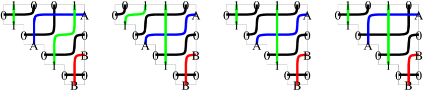
Figure 1. The IP pipe dreams whose partial permutation is $1\mapsto 2,3\mapsto 4$. (The lettered pipes connect the $1$st and $3$rd East edges to the $2$nd and $4$th South edges.) Note that in the first and fourth figures, the $A$ pipe crosses a $0$ pipe twice, but that’s permissible because the $0$ isn’t a lettered pipe.

Each lettered pipe connects a horizontal edge below the diagonal to a vertical edge on the East side. Since $a\neq b$ in crossing tiles, the $i$th $-\!\!\!-\!\!\!\!\!\!\!\!B\ \,$ from the left must connect to the $i$th $\,\big{|}\!\!\!B$ from the top. By the nonlocal condition, the $i$th $A$ pipe will cross the $j$th $B$ pipe either once or not at all, and can be predicted from the boundary and the Jordan curve theorem.

We think of two IP pipe dreams as equivalent if they differ only in the letter labels. This includes the possibility of folding two letters into the same letter (only allowed if those pipes don’t cross, which as just explained can be predicted from the boundary).

To an IP pipe dream $P$, we associate two objects:

• $f(P)$, an upper triangular partial permutation depending on only
  the South and East labels of $P$, and

• $\lambda(P)$, a partition depending on only the North labels.

The partial permutation $f(P)$ is induced by the lettered pipes, (i.e. not labeled $0,1$), as follows. For each lettered pipe in $P$, place a $1$ in $f(P)$ above the South end of the pipe, and left of the East end. In particular, the $1$s coming from pipes of a given letter are arranged NW/SE (since such pipes don’t cross). The IP pipe dreams in figure 1 are all those with $f(P)$ being the partial permutation $1\mapsto 2,3\mapsto 4$.

The English partition $\lambda(P)$ in the fourth quadrant of the Cartesian plane is read as follows. Start at the point $(0,\#0$s across the North side$)$ and reading the North side of $P$ from left to right, move down for each $1$, and left for each $0$. The region above the resulting path is the partition $\lambda(P)$, and $\dim X^{\lambda(P)}=|\lambda(P)|$. As we will see later, $|\lambda(P)|+|\mu|=|\nu|+\#$equivariant tiles in $P$. In the IP pipe dreams in figure 1, the partitions are $(2)={\tiny\hbox{}{\vbox{\offinterlineskip\vbox{\hrule height=0.3pt\hbox{\vrule height=4.37334pt,width=0.3pt,depth=1.0933pt\hbox to5.46666pt{\hfil}\vrule height=4.37334pt,width=0.3pt,depth=1.0933pt\hbox to5.46666pt{\hfil}\vrule height=4.37334pt,width=0.3pt,depth=1.0933pt} \hrule height=0.3pt}\vspace{-\y@linethick} }}},(1,1)={\tiny\hbox{}{\vbox{\offinterlineskip\vbox{\hrule height=0.3pt\hbox{\vrule height=4.37334pt,width=0.3pt,depth=1.0933pt\hbox to5.46666pt{\hfil}\vrule height=4.37334pt,width=0.3pt,depth=1.0933pt} \hrule height=0.3pt}\vspace{-\y@linethick} \vbox{\hrule height=0.3pt\hbox{\vrule height=4.37334pt,width=0.3pt,depth=1.0933pt\hbox to5.46666pt{\hfil}\vrule height=4.37334pt,width=0.3pt,depth=1.0933pt} \hrule height=0.3pt}\vspace{-\y@linethick} }}},(1)={\tiny\hbox{}{\vbox{\offinterlineskip\vbox{\hrule height=0.3pt\hbox{\vrule height=4.37334pt,width=0.3pt,depth=1.0933pt\hbox to5.46666pt{\hfil}\vrule height=4.37334pt,width=0.3pt,depth=1.0933pt} \hrule height=0.3pt}\vspace{-\y@linethick} }}},(1)={\tiny\hbox{}{\vbox{\offinterlineskip\vbox{\hrule height=0.3pt\hbox{\vrule height=4.37334pt,width=0.3pt,depth=1.0933pt\hbox to5.46666pt{\hfil}\vrule height=4.37334pt,width=0.3pt,depth=1.0933pt} \hrule height=0.3pt}\vspace{-\y@linethick} }}}$ respectively.

Theorem 1.1.

In $H^{*}_{T}(Gr_{k}({\mathbb{A}}^{n}))$, expanding $[\Pi_{f}]$ in the $\mathbb{Z}$-basis of opposite Schubert classes gives

$$[\Pi_{f}]=\sum_{P:f(P)=f\atop\text{ $P$ has no equivariant tiles}}[X^{\lambda(P)}]\quad=\quad\sum_{\lambda}\#\bigg{\{}P\ :\ {f(P)=f,\ \lambda(P)=\lambda\atop\text{ $P$ has no equivariant tiles}}\bigg{\}}\ [X^{\lambda}].$$

Let $T\leq GL(n)$ be the diagonal matrices. As $\Pi_{f}$ is preserved by this group, it defines a class in $H^{*}_{T}(Gr_{k}({\mathbb{A}}^{n}))$, again denoted $[\Pi_{f}]$. The corresponding expansion in the basis requires coefficients from $H^{*}_{T}(pt)\cong Sym(T^{*})\cong\mathbb{Z}[y_{1},\ldots,y_{n}]$, where $y_{i}$ is the character $y_{i}({\rm diag}(t_{1},\ldots,t_{n}))=t_{i}$ on $T$.

Define $wt(P)\in H^{*}_{T}(pt)$ (for “weight”) as the product of $y_{row(t)}-y_{col(t)}$, over all equivariant tiles $t$. In the IP pipe dreams in figure 1, the weights are $1,1,y_{1}-y_{2},y_{2}-y_{4}$ respectively.

Theorem 1.2.

In $H^{*}_{T}(Gr_{k}({\mathbb{A}}^{n}))$, expanding $[\Pi_{f}]$ in the $H^{*}_{T}(pt)$-basis of opposite Schubert classes gives

$$[\Pi_{f}]=\sum_{P:\ f(P)=f}wt(P)\ [X^{\lambda(P)}].$$

Specializing each $y_{i}$ to $0$ recovers the previous theorem.

This formula is manifestly Graham-positive [Gr00]. In the figure 1 example, it says

$$[\Pi_{1\mapsto 2,\ 3\mapsto 4}]=[X^{(2)}]+[X^{(1,1)}]+(y_{1}-\cancel{y_{2}}+\cancel{y_{2}}-y_{4})[X^{(2,1)}]\qquad\in H^{*}_{T}(Gr_{k}({\mathbb{A}}^{n})).$$

1.3. Shifting and sweeping

In this paper “variety” means “reduced and irreducible scheme”, and any “subvariety” will be closed. Also, $[n]$ denotes $\{1,2,\ldots,n\}$.

Let $X$ be a $T$-invariant subvariety of $Gr_{k}({\mathbb{A}}^{n})$, and for $i,j\in[n]$ define the (geometric) shift of $X$

$$\textcyr{X}_{i\to j}X:=\lim_{t\to\infty}\exp(te_{ij})\cdot X$$

where $e_{ij}$ is the matrix with a $1$ at $(i,j)$ and $0$s elsewhere. (The precise definition of such a limit is recalled in §3.) Then the limit scheme $\textcyr{X}_{i\to j}X$ is again $T$-invariant, and defines the same homology and $K$-class as $X$ itself. I learned of this construction from [Va06], but as we explain in §3, it is closely related to the Erdős-Ko-Rado shifting construction [EKR61] in extremal combinatorics.

To keep track of the equivariant class, we also need the (geometric) sweep of $X$,

$$\Psi_{i\to j}X:=\overline{\bigcup_{t\in{\mathbb{A}}^{1}}\ \exp(te_{ij})\cdot X}$$

For general $X$, these schemes can be very difficult to compute; we give some general results in §3. But certain shifts of certain interval positroid varieties are tractable.

Call $(i,j)$ an essential box for the partial permutation $f$ if its rank condition $r(M)_{ij}\leq r(f)_{ij}$ is not implied by the rank condition for any of $(i\pm 1,j),(i,j\pm 1)$. (There is an easy combinatorial description of these from [Fu92], recalled in §2.) Call a shift $(i,j)$ safe for $f$ if for each essential box $(i^{\prime},j^{\prime})$, either $i\in[i^{\prime},j^{\prime}]$, or $j\notin[i^{\prime},j^{\prime}]$, or $(i^{\prime},j^{\prime})=(i+1,j)$.

Theorem 1.3.

If the shift $(i,j)$ is safe for $f$, then $\Psi_{i\to j}\Pi_{f}$ is again an interval positroid variety, and $\textcyr{X}_{i\to j}\Pi_{f}$ is a certain reduced union $\bigcup_{f^{\prime}\in C}\Pi_{f^{\prime}}$ of interval positroid varieties. If $(i+1,j)$ is indeed an essential box for $f$, then

$$[\Pi_{f}]=(y_{i}-y_{j})\big{[}\Psi_{i\to j}\Pi_{f}\big{]}+\sum_{f^{\prime}\in C}[\Pi_{f^{\prime}}]$$

as elements of $H^{*}_{T}(Gr_{k}({\mathbb{A}}^{n}))$. If $(i+1,j)$ is not an essential box for $f$, then $\Pi_{f}$ is $\textcyr{X}_{i\to j}$-invariant, in that $\textcyr{X}_{i\to j}\Pi_{f}=\Psi_{i\to j}\Pi_{f}=\Pi_{f}$.

If $f=f(P)$ for an IP pipe dream using $m$ distinct letters, then $\textcyr{X}_{i\to j}\Pi_{f}$ has at most $m+1$ components. The intersection of any set $S\subseteq C$ of these components is again an interval positroid variety $\Pi_{f(S)}$. In particular, as $K$-classes,

$$[\Pi_{f}]=[\textcyr{X}_{i\to j}\Pi_{f}]=\bigg{[}\bigcup_{f^{\prime}\in C}\Pi_{f^{\prime}}\bigg{]}=\sum_{S\subseteq C,\ S\neq\emptyset}(-1)^{|S|-1}\ [\Pi_{f(S)}].$$

The precise version of the theorem (enumerating the components in $C$) will be theorem 3.15, which also includes the extension to $K_{T}(Gr_{k}({\mathbb{A}}^{n}))$.

1.4. The Vakil sequence

Given an IP pipe dream $P$, and a box $(i,j),i\leq j$, define (as in figure 2) the slice $s(P,i,j)$ of $P$ at $(i,j)$ as the data of the labels on

• the South edges of $\{(m,m):m<i\}\ \cup\ \{(i,m):i\leq m\leq j\}\ \cup\ \{(i-1,m):j<m\leq n\}$

• the East edges of $(i,j)$ and $\{(m,n):m<i\}$.

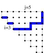
Figure 2. An $n=6$ example of a slice at $(3,5)$. The slice is the thick blue edges and the (unpictured) labels thereon.

Not every labeling $s$ of these edges arises from an IP pipe dream; we spell out the conditions in §4. To each “viable” slice $s$, we associate in §4 a partial permutation $f(s)$. For now, it suffices to mention that $f(s(P,n,n))=f(P)$, and $\Pi_{f(s(P,1,1))}=X^{\lambda(P)}$.

Given a slice $s$, we can consider what tiles can be placed at $(i,j)$, making new slices $s^{\prime}$ at $(i,j-1)$ (or at $(i-1,n)$ if $j=i$).

Theorem 1.4.

Let $s$ be a slice at $(i,j)$, and $\Pi_{f(s)}$ the associated interval positroid variety (defined in §4). The shift $(i,j)$ is safe for $f(s)$. Let $\{s^{\prime}\}$ be the set of viable slices arising from a tile at $(i,j)$.

1. If the South and East labels of $(i,j)$ in $s$ are not both zero, then $\Pi_{f(s)}$ is $\textcyr{X}_{i\to j}$-invariant. There is a unique $s^{\prime}$, and its $f(s^{\prime})$ is unchanged from $f(s)$.

   1. If the labels are equal but not $0$, forcing the $a=0$ elbows tile, then $f(s)\big{(}i\big{)}=j$.

   2. If the labels are distinct, forcing the crossing tile, then $f(s)\big{(}i\big{)}\neq j$ (and is undefined if the East label is $0$).

2. If the South and East labels of $(i,j)$ in $s$ are both $0$, then the various $\{\Pi_{f(s^{\prime})}\}$ are the sweep (for the equivariant tile) and the components of the shift (for the other possible tiles).

This is the inductive step by which theorem 1.2 is proved, where $i$ decreases from $n$ to $1$, and for each $i$ we take $j$ from $n$ down to $i+1$. This is exactly the sequence of shifts used in [Va06, §2.2], though Vakil doesn’t use the shifting formalism.

1.5. Extension to $K$-theory

1.5.1. The $K$-tiles

To compute in equivariant $K$-theory, we need a new kind of label $W$ on the vertical edges: it is a word in $\{1\}\cup\{A,B,\ldots\}$ (no $0$s), no letters repeating, and if it contains $1$ then the $1$ must be at the end. There are now four kinds of tiles, including the fundamentally new “displacer” tile:

Define a $K$-IP pipe dream as one built from these tiles, with the same conditions as on an IP pipe dream, plus one more nonlocal condition: two pipes appearing in the same word must cross once (and, of course, not twice). The meeting of two pipes in a fusor or displacer tile doesn’t count as a crossing. Note that IP pipe dreams are a subclass of $K$-IP pipe dreams, where $|W|=1$ in the crossing tiles, $|W|=0$ in the fusor tiles, and there are no displacer tiles.

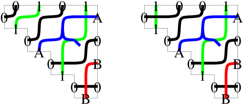
Figure 3. The $K$-IP pipe dreams whose partial permutation is $1\mapsto 2,3\mapsto 4$ that didn’t appear in figure 3. Each fuses an $A$ and a $1$ pipe, at $(2,4)$.

Notice that if, on each edge of a $K$-IP pipe dream we erase every label except the last one, we get a consistent system of unbroken pipes, and missing labels can be reconstructed uniquely from the visible ones. However, the nonlocal conditions that say which systems of pipes can be extended to a $K$-IP pipe dream seem too complicated to be useful.

As theorem 1.3 suggests, there are signs in the $K$-formula, but (as predicted by Brion’s theorem [Bri02]) they are determined by the parity of the codimension. Let $fusing(P)$ denote the sum over the fusor tiles, of the size $|W|$ of their word. (So $fusing(P)=0$ iff the $K$-IP pipe dream $P$ is an ordinary IP pipe dream, since the presence of a displacer tile forces the appearance of a fusor tile with $|W|>0$ to the East of it.)

Theorem 1.5.

In $K^{*}(Gr_{k}({\mathbb{A}}^{n}))$, expanding $[\Pi_{f}]$ in the $\mathbb{Z}$-basis of opposite Schubert classes gives

$$[\Pi_{f}] = \sum_{P:\ f(P)=f\atop\text{ $P$ has no equivariant tiles}}(-1)^{fusing(P)}[X^{\lambda(P)}]$$

$$= \sum_{\lambda}(-1)^{\dim\Pi_{f}-\dim X^{\lambda}}\#\bigg{\{}P\ :\ {f(P)=f,\ \lambda(P)=\lambda\atop\text{ $P$ has no equivariant tiles}}\bigg{\}}\ [X^{\lambda}].$$

If $P$ is a $K$-IP pipe dream, then $fusing(P)=\dim\Pi_{f(P)}-\dim X^{\lambda(P)}$, so this formula is positive in the sense of [Bri02].

Combining the nonequivariant pipe dreams from figures 1 and 3, we get

$$[\Pi_{1\mapsto 2,3\mapsto 4}]=[X^{(2)}]+[X^{(1,1)}]-[X^{(1)}]\qquad\in K(Gr_{k}({\mathbb{A}}^{n})).$$

Notice that as compared to $H^{*}$, the extra terms in $H^{*}_{T}$ come from larger varieties $X^{\lambda}$, whereas the extra terms in $K$ come from smaller varieties.

1.5.2. $T$-equivariance

The base ring $K_{T}(pt)$ of $T$-equivariant $K$-theory is the Laurent polynomial ring $Rep(T)\cong\mathbb{Z}[\exp(\pm y_{1}),\ldots,\exp(\pm y_{n})]$, written thus for comparison to equivariant cohomology. Here $\exp(y_{i})$ denotes the $K_{T}$-class of the one-dimensional representation with character $y_{i}$.

Define the $K_{T}$-weight $wt_{K}(P)$ of a $K$-IP pipe dream as

$$wt_{K}(P):=\prod_{i<j}\begin{cases}1-exp(y_{j}-y_{i})&\text{ if the tile at $(i,j)$ is the equivariant tile (all $0$s)}\\ \phantom{0}+exp(y_{j}-y_{i})&\text{ if the tile at $(i,j)$ has $0$s on its South and East only}\\ 1\phantom{0+1}&\text{ otherwise}.\end{cases}$$

The special role of the tiles with $0$ on the South and East becomes clear in §4.3.

Theorem 1.6.

In $K_{T}^{*}(Gr_{k}({\mathbb{A}}^{n}))$, the expansion of $[\Pi_{f}]$ in the $\mathbb{Z}[\exp(\pm y_{1}),\ldots,\exp(\pm y_{n})]$-basis of opposite Schubert classes is

$$[\Pi_{f}]=\sum_{P:\ f(P)=f}(-1)^{fusing(P)}wt_{K}(P)\ [X^{\lambda(P)}]$$

which is positive in the sense predicted in [AGriMil11, Corollary 5.1].

Specializing each $y_{i}=0$ recovers the previous theorem. Dropping the $fusing(P)>0$ summands, and taking the lowest-degree term in the $(y_{i})$, recovers the $H^{*}_{T}$-formula from the $K_{T}$.

For example, the $K_{T}$-weights of the $K$-IP pipe dreams from figures 1 and 3 are (in order)

$$\exp(y_{2}-y_{4}),\qquad\exp(y_{1}-y_{2}),\qquad 1-\exp(y_{1}-y_{2}),\qquad 1-\exp(y_{2}-y_{4}),$$

$$\exp(y_{1}-\cancel{y_{2}}+\cancel{y_{2}}-y_{4}),\qquad(1-\exp(y_{1}-y_{2}))\exp(y_{2}-y_{4})=\exp(y_{2}-y_{4})-\exp(y_{1}-y_{4}).$$

1.6. Outline of the paper

In §2 we recall the basic properties we need of interval positroid varieties, and in particular define their essential and crucial boxes. In §3 we give some results about geometric and combinatorial shifting, and prove theorem 1.3 about safe shifts of positroid varieties. In §4 we prove the main theorem, that $K$-IP pipe dreams serve as a record of the degeneration process defined by Vakil [Va06], in enough detail to recover the $K_{T}$-class. In §5 we connect IP pipe dreams to the equivariant puzzles of [KnTao03].

The combinatorial difference between the pipe dream calculus laid out here, as contrasted with the checker games of [Va06], is that an IP pipe dream serves as a $2$-dimensional record of a $(2+1)$-dimensional checker game.

2. Interval positroid varieties

Most of the definitions in this section (though not the one in its title) are from [KLS13].

2.1. Positroid varieties and their covering relations

A juggling pattern of length $n$ is a bijection $J:\mathbb{Z}\to\mathbb{Z}$ such that $f(i)-i$ is periodic with period $n$, and $f(i)-i\geq 0$ for all $i\in\mathbb{Z}$. The siteswap of $J$ is the $n$-tuple $f(1)-1,\ldots,f(n)-n$, and obviously $J$ can be reconstructed from its siteswap. The average $k$ of the siteswap turns out to be the number of orbits of $J$ that aren’t fixed points, called the ball number. Hereafter fix $n$ and $k$.

Call $J$ bounded if $f(i)-i\leq n$ for all $i\in\mathbb{Z}$. For such $J$, define the following variety ${\widetilde{\Pi}}_{J}\subseteq M_{k\times n}$ by rank conditions on all cyclic intervals:

$$r(J)_{ij} := \big{|}[i,j]\big{|}-\#\{\text{$1$s in $J$'s matrix that are weakly Southwest of $(i,j)$}\},\quad i\leq j\leq i+n$$

$${\widetilde{\Pi}}_{J} := \{M:\ M\in M_{k\times n},\ {\rm rank}(\text{columns }[i,j]\bmod n)\leq r(J)_{ij},\quad\forall i\in\mathbb{Z},j\in[i,i+n]\}$$

The positroid variety $\Pi_{J}\subseteq Gr_{k}({\mathbb{A}}^{n})$ is defined as

$$\Pi_{J}:=\{{\rm rowspan}(M):M\in{\widetilde{\Pi}}_{J},\ {\rm rank}(M)=k\}.$$

All the properties claimed in §1.1 of interval positroid varieties are in fact true of positroid varieties, as proven in [KLS13, §5.4–5.5].

We depict $J$ as an infinite, periodic permutation matrix, with dots in the boxes $(i,J(i))$, $i\in\mathbb{Z}$. To construct the diagram of $J$, we cross out all boxes strictly to the West or South (but not both) of each dot, leaving the diagram as the remainder. The essential set ${\rm ess}(J)$ is the set of Northeast corners of the diagram (note that the diagram has one unbounded component, stretching North and East to infinity with no Northeast corner). It is not difficult to prove (in analogy with [Fu92]) that

$${\widetilde{\Pi}}_{J}=\{M:\ M\in M_{k\times n},\ {\rm rank}(\text{columns }[i,j]\bmod n)\leq r(J)_{ij},\quad\forall(i,j)\in{\rm ess}(J)\}.$$

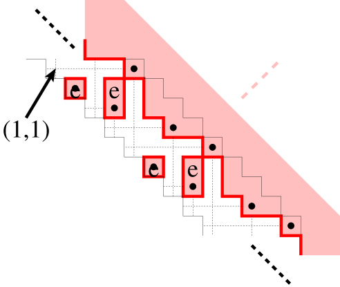
Figure 4. The diagram of the juggling pattern with siteswap $4013$, in pink. Up to $4$-periodicity, it has two essential boxes, at $(2,2)$ and $(2,4)$, whose associated rank conditions are ${\rm rank}[$column $2]\leq 0$, ${\rm rank}[$columns $2,3,4]\leq 1$.

More specifically, the “essential” set of rank conditions are those that are not implied by single other rank conditions. In matroid terminology, a rank condition not implied by one from a larger subset is a flat, and a rank condition not implied by one from a smaller subset is cyclic (a union of “circuits”); don’t confuse this with our “cyclic intervals”! The cyclic flats are of additional interest because they form a lattice [BdM08]. (There is a slight confusion that the whole $[n]$ may be a cyclic flat, but will not be an “essential” interval.)

However, it is possible for a cyclic flat’s condition to be implied by a combination of other conditions, in two ways. If $F=F_{1}\coprod F_{2}$ and ${\rm rank}(F)={\rm rank}(F_{1})+{\rm rank}(F_{2})$, then $F$ is called not connected. (Example: let $k=3$, $n=6$,

$$J(i)=\begin{cases}i+5&\text{$i$ odd}\\ i+1&\text{$i$ even.}\end{cases}$$

Then $[1,4]=[1,2]\coprod[3,4]$ is not connected. Again, don’t confuse this with “contiguous”, which the numbers $[1,4]$ certainly are!) The same can happen in the dual matroid, in which case $F$ is not nnected. Following [FoS], call the rank conditions associated to the connected and nnected flats of a matroid the crucial conditions.

The positroid varieties form a stratification of $Gr_{k}({\mathbb{A}}^{n})$, and a ranked poset where the rank is given by the dimension of the variety. More specifically, the assignment $\Pi_{J}\mapsto J$ gives an anti-isomorphism of this poset to an order ideal in affine $S_{n}$ Bruhat order [KLS13, Theorem 3.16]. In this poset, we have a covering relation $J\gtrdot J^{\prime}$ iff $J,J^{\prime}$ agree away from rows $i$ and $j$ (mod $n$), if the dot $(i,J^{\prime}(i))$ is Northeast of the dot $(j,J^{\prime}(j))$ (which is well-defined, even with periodicity), and there are no dots in $J$ or $J^{\prime}$ in the interior of the rectangle with those as Northeast and Southwest corners. Also, the difference $r(J)-r(J^{\prime})$ of the rank functions is an upper triangular periodic matrix of $0$s and $1$s, with $1$s in the rectangle $[i+1,j]\times[J(i),J(j)-1]$ (and its periodic copies).

2.2. Several classes of positroid varieties, including interval

Because of its periodicity, the affine permutation matrix of a bounded juggling pattern $J$ is determined by what it does in rows $i=1,\ldots,n$, whose intersection with the strip $i\leq j\leq i+n$ is a parallelogram. Cut it into a left half ($j\leq n$) and right half ($j>n$). We can pick out several important classes of positroid varieties, with decreasing specificity:

• Opposite Schubert varieties. If the dots run NW/SE in the entire parallelogram.

• Richardson varieties. If the dots run NW/SE in each of the two triangular halves.

• Interval positroid varieties. If the dots run NW/SE in the right half.

We now prove these characterizations, starting with the third.

Proposition 2.1.

If $\Pi_{f}$ is the interval positroid variety associated with the partial permutation $f$, then there exists a unique bounded juggling pattern $J(f)$ such that $\Pi_{f}=\Pi_{J(f)}$. Moreover, $J(f)$’s permutation matrix is characterized by having $f$ on the triangle $1\leq i\leq j\leq n$, and has $k$ dots arranged NW/SE on the triangle $i\leq n<j\leq i+n$.

Proof.

Call the two triangles “$f$’s triangle” and “the second triangle”. Let $C_{f},R_{f}\in{[n]\choose n-k}$ be the set of nonzero columns and rows of $f$. Then $C_{f}\geq R_{f}$ in Bruhat order, by the condition that $f$ is upper triangular.

We need to construct $J:=J(f)$. Copy $f$ into $f$’s triangle, and cross out the complete row and column of each of $f$’s $n-k$ dots. The square $i\in[1,n],j\in[n+1,2n]$ will have $k$ remaining rows and columns, $r_{1}<r_{2}<\ldots<r_{k}\subseteq[1,n],c_{1}<\ldots<c_{k}\subseteq[n+1,2n]$. We’ll place dots NW/SE so in matrix entries $(r_{i},c_{i})$, $i=1\ldots k$, and copy them periodically to $(r_{i}+Mn,c_{i}+Mn),M\in\mathbb{Z}$.

Now we claim that for each $i$, $c_{i}-n\leq r_{i}$, i.e. that the $J$ so constructed is a bounded juggling pattern. To see this, let $R^{\prime}_{f}=[n]\setminus R_{f}$ be the rows of the new dots, and $C^{\prime}_{f}=[n]\setminus C_{f}$ be the columns minus $n$. Since $C_{f}\geq R_{f}$, we learn $C^{\prime}_{f}\leq R^{\prime}_{f}$, i.e. $c_{i}-n\leq r_{i}$ for each $i$.

To show $\Pi_{f}=\Pi_{J}$, we will show there are no crucial rank conditions in the second triangle. Let $(i,j+n)$ be an “essential” box there, corresponding to the cyclic interval $[i,j]:=[i,n]\coprod[1,j]$. (Note that $j<i-1$, since the box $(i-1,j+n)$ North of $(i,j+n)$ must both be crossed out by some dot strictly to its East $(i-1,j+n+m)$, so $j+1\leq j+m\leq i-1$.) Then since there are no dots Southwest of $(i,j+n)$ in the second triangle (by the NW/SE condition), its rank condition is

$$r(M)_{ij} = |[i,n]|+|[1,j]|-\#\{\text{dots in $J$ that are weakly Southwest of $(i,j+n)$}\}$$

$$= |[i,n]|+|[1,j]|-\#\{\text{weakly SW of $(i,n)$}\}-\#\{\text{weakly SW of $(1+n,j+n)$}\}$$

$$= r(M)_{in}+r(M)_{1j}$$

so the cyclic flat $[i,n]\coprod[1,j]$ is not a connected flat. ∎

If $J$’s crucial conditions are all intervals, not just cyclic intervals, then $\Pi_{J}$ is obviously an interval positroid variety as defined in §1.1. The example given in the last section, whose crucial intervals are $[1,2],[3,4],[5,6]$ show that the “essential” cyclic intervals may be properly cyclic ($[5,2]$ in that example).

This construction suggests we define the diagram of a partial permutation $f$ by crossing out strictly West and South from each dot, and also crossing out entirely any row or column with no dot (as secretly, that dot is hiding in the second triangle of $J(f)$). Then as before, $f$’s “essential” boxes are the Northeast corners of the diagram.

The following is essentially well-known; we only include it to fix notation.

Lemma 2.2.

If $f$’s dots are in the first $n-k$ rows, running NW/SE, then $\Pi_{f}=X^{\lambda}$ where the partition $\lambda$ is constructed from $f$’s columns, read backwards, as follows: Start at the point $(0,-k)$ in the fourth quadrant of the Cartesian plane, and move right for each nonzero column, and up for each zero column.

Proof.

Crossing out South and East from $f$’s dots, and crossing out the $k$ empty rows beneath, already only leaves a partition in the Northeast corner. Crossing out empty columns cuts that into a bunch of partitions, each of which reach up to the top row. Hence the essential conditions are all on intervals $[1,j]$, and so define an opposite Schubert variety, easily checked to be this one. ∎

Lemma 2.3.

Let $f$ be the left half of $J$’s parallelogram. The unique smallest Richardson variety containing $\Pi_{J}$ is $X_{\mu}\cap X^{\nu}$, where $\nu$ is constructed from $f$’s nonzero columns as in lemma 2.2, and $\mu$ by using $f$’s nonzero rows. The containment $X_{\mu}\cap X^{\nu}\supseteq\Pi_{J}$ is an equality iff the dots run NW/SE in each of the left and right halves of $J$’s parallelogram.

Proof.

First we check straightforwardly that the smallest Schubert and opposite Schubert varieties containing $\Pi_{J}$ are $X_{\mu}$ and $X^{\nu}$, by checking the rank conditions on the intervals $\{[i,n]\}$ and $\{[1,j]\}$.

Since Schubert and opposite Schubert varieties are positroid varieties, so are Richardson varieties. So the containment $X_{\mu}\cap X^{\nu}\supseteq\Pi_{J}$ is an equality exactly if $\Pi_{J}$ is the largest positroid variety with these given rank conditions on the intervals $\{[i,n]\}$ and $\{[1,j]\}$.

If $\Pi_{J}$ has a NE/SW pair of dots in either the left or right half, with the NE dot minimally NE of the SW dot, we can switch them for a NW/SE pair by doing a covering relation in affine Bruhat order. This terminates when we can’t get bigger inside $X_{\mu}\cap X^{\nu}$, and also when there are no such pairs, as was to be shown. ∎

Given $X\subseteq Gr_{k}({\mathbb{A}}^{n})$, let ${\widetilde{X}}\subseteq M_{k\times n}$ be the closure of $\{M\in M_{k\times n}:{\rm rowspan}(M)\in X\}$, and call it the Stiefel cone over $X$. (We invented this terminology to generalize the “affine cone” $k=1$ case, and the Stiefel manifold.) When $k=1$ this is the usual affine cone over a projective variety. Because of the closure operation, the Stiefel cone may be more singular than $X$ itself. Of course our interest is in the case $X=\Pi_{J}$, where ${\widetilde{X}}={\widetilde{\Pi}}_{J}$.

Proposition 2.4.

Let $f$ be an $n\times n$ upper triangular partial permutation matrix of rank $n-k$. Construct $f^{\prime}$ of size $(n+k)\times(n+k)$ of rank $n$, by putting $f$ in the upper left corner, $k$ zero rows on the bottom, and $k$ dots arranged NW/SE in the remaining $n\times k$ rectangle in the NE. Then ${\widetilde{\Pi}}_{J(f)}$ is isomorphic to an open set on $\Pi_{J(f^{\prime})}$. Hence each ${\widetilde{\Pi}}_{J(f)}$ is normal and Cohen-Macaulay, with rational singularities, and intersections of unions of these Stiefel cones are reduced.

Proof.

The correspondence is $M\mapsto{\rm rowspan}[M\ {\rm Id}_{k}]$, landing inside the big cell in which the last Plücker coordinate is nonzero. ∎

These good properties do not hold for the Stiefel cones ${\widetilde{\Pi}}_{J}$ of general positroid varieties. In particular, if the Stiefel cones over the four positroid divisors in $Gr_{2}({\mathbb{A}}^{4})$ are $D_{1},D_{2},D_{3},D_{4}$, then the scheme $D_{1}\cap D_{2}\cap(D_{3}\cup D_{4})$ contains the rank $\leq 1$ matrices as a component of multiplicity $2$ (so, nonreduced). From this point of view, the Stiefel cones of positroid varieties behave as badly as one would expect them to, and the Stiefel cones of interval positroid varieties are only better behaved because they are open sets on positroid varieties.

This next proposition computes the $T$-fixed points on an interval positroid variety, in terms of matchings. (It will not be used later.)

Proposition 2.5.

Let $f$ be an upper triangular $n\times n$ partial permutation matrix, and $S\subseteq[n]$ a subset. Let $dots(f)=\{(i,f(i)):f(i)$ defined$\}$. Then $\Pi_{f}$ contains the coordinate space ${\mathbb{A}}^{S^{c}}$ that uses the coordinates not in $S$ if and only if there is a matching $m:dots(f)\to S$, where $a\leq m(a,b)\leq b$ for each $(a,b)\in dots(f)$.

In words, each dot $(a,b)$ gets matched with a diagonal entry $(m,m)$ to its Southwest, with $S$ the unmatched part of the diagonal.

Proof.

Let $n-k$ be the rank of $f$, so by definition, $\Pi_{f}\subseteq Gr_{k}({\mathbb{A}}^{n})$, and any coordinate space in it must be $k$-dimensional. Thus already $S$ must have size $n-k$.

By the definition of $\Pi_{f}$, it contains ${\mathbb{A}}^{S^{c}}$ iff for each interval $[i,j]$,

$$\big{|}[i,j]\setminus S\big{|}\ \ \leq\ \ \big{|}[i,j]\big{|}-\#\left\{(a,b)\in dots(f):i\leq a\leq b\leq j\right\}$$

or equivalently

$$\big{|}[i,j]\cap S\big{|}\ \ \geq\ \ \#\left\{(a,b)\in dots(f):i\leq a\leq b\leq j\right\}\quad=:\#dots_{\swarrow(i,j)}(f).$$

If a matching $m$ exists, it gives an injection of the set on the right to the set on the left. That proves one direction.

We will refer to each of these as an “$[i,j]$ inequality”. Assume that each $[i,j]$ inequality holds; we need to construct a matching.

If $f(h)=h$ (i.e. we have a dot on the diagonal), then the $[h,h]$ inequality shows $h\in S$, and the matching must include $(h,h)\mapsto h$. If we remove the dot from $f$ and $h$ from $S$, producing the new matching problem $f^{\prime},S^{\prime}$, then any interval $[i,j]\ni m$ will have both sides of its inequality decrease by $1$, and any interval $[i,j]\not\ni m$ will stay exactly the same. In particular, the new problem $f^{\prime},S^{\prime}$ satisfies the required inequalities, so has a solution by induction on ${\rm rank}(f)$. With this we reduce to the case that $f$ has no dots on the diagonal. In particular, being strictly upper triangular, it must have some columns without dots. If $f$ is the zero matrix, we are done, so assume otherwise.

Let $j+1$ be the leftmost column with a dot, say at $(i,j+1)$. We will try (and possibly fail – this remains to be seen) to move that dot West to $(i,j)$, producing $f^{\prime}$. This increases the right-hand side of each $[h,j]$ inequality. If they all still hold, then we can use a matching $m^{\prime}$ for $f^{\prime}$ to build a matching $m$ for $f$, by composing with the correspondence between the dots of $f$ and $f^{\prime}$.

If some $[h,j]$ inequality does not hold for $f^{\prime}$, obstructing this move, it is because

$$\big{|}[h,j]\cap S\big{|}\ \ =\ \ \#dots_{\swarrow(h,j)}(f).$$

Compare with the $[h,j+1]$ inequality; the right side is $1$ dot larger, so the left side must have $1$ more element of $S$, i.e. $j+1\in S$. So instead of moving the $(i,j+1)$ West, we will try to match it up with $j+1\in S$. (This time, we will be successful.) Let $f^{\prime},S^{\prime}$ be $f,S$ with $(i,j+1)$ and $j+1$ removed.

This decreases the left side of various $[a,b]$ inequalities, and the right side of others. The only bad possibility is that we decrease the left side, but not the right, for some $[a,b]$ inequality that held with equality. The left side decreases if $[a,b]\ni j+1$. The right side stays the same if $[a,b]\not\supseteq[i,j+1]$. Hence $i<a\leq j+1\leq b$.

Let $c$ be the number of dots in the rectangle $[i,a-1]\times[j+1,b]$; we know $c>0$ because of dot $(i,j)$.

$$\left|S\cap[a,j]\right| = \left|S\cap[i,j]\right|+\left|S\cap[a,b]\right|-\left|S\cap[i,b]\right|$$

$$= \#dots_{\swarrow(i,j)}(f)+\#dots_{\swarrow(a,b)}(f)-\left|S\cap[i,b]\right|$$

$$\leq \#dots_{\swarrow(i,j)}(f)+\#dots_{\swarrow(a,b)}(f)-\#dots_{\swarrow(i,b)}(f)$$

$$= \#dots_{\swarrow(a,j)}(f)-c$$

$$< \#dots_{\swarrow(a,j)}(f)$$

but this contradicts the $[a,j]$ inequality. So there is no obstruction to starting the matching with $(i,j+1)\mapsto j+1$. ∎

If $X\subseteq Gr_{k}({\mathbb{A}}^{n})$ is $T$-invariant and irreducible, its matroid is the collection $B(X):=\{S\subseteq[n]:{\mathbb{A}}^{S}\in X\}$. A positroid is one arising from $X=\overline{T\cdot V}$ where $V$ has all nonnegative real Plücker coordinates [Pos]. The matroids of the $\{\Pi_{f}\}$ are positroids, whose connected flats are intervals (not just cyclic intervals), hence the term “interval positroid variety”.

Under Grassmannian duality $Gr_{k}({\mathbb{A}}^{n})\cong Gr_{n-k}({\mathbb{A}}^{n})$, one can check that the positroid variety $\Pi_{f}$ is corresponded with the positroid variety $\Pi_{(i\mapsto i+n)\circ f^{-1}}$. This does not preserve the subclass of interval positroid varieties (other than the Richardson varieties). The additional power available from dualizing is exploited in [KnLed].

One interpretation of proposition 2.5 is that interval positroids are “dual transversal” matroids. Consider the dots in $f$ as a set of $n-k$ choosy brides $b$, each of whom will only marry a groom within a certain height range $[i_{b},j_{b}]$. Then each $S$ is an acceptable set of grooms. Hall’s Marriage Theorem (from which this terminology is derived) says that if some groomset $S\subset[n],|S|={\rm rank}(f)$ is unmarriable, it is because there is a set $B$ of brides with $\left|S\cap\cup_{(i,j)\in B}[i,j]\right|<|B|$. Proposition 2.5 goes further in two ways: it says that if $S$ is unmarriable, then (1) there is an interval $[a,b]$ where $B$ is the brides with ranges in that interval, and the grooms in that interval aren’t numerous enough, (2) even if one includes the grooms none of those brides wants.

2.3. A Monk formula for positroid varieties

For $S\subseteq[n]$, $r\in{\mathbb{N}}$, let

$$X_{S\leq r}:=\{{\rm rowspan}(M):M\in M_{k\times n},{\rm rank}\ M=k,{\rm rank}\ (\text{columns $S$ of }M)\leq r\}.$$

If $S$ is a cyclic interval, call this a basic positroid variety. Clearly every positroid variety is an intersection of basic ones, and one can show that no basic positroid variety is an intersection of other positroid varieties.

Theorem 2.6.

Let $J$ be a bounded juggling pattern, and $\big{(}i,j=J(i)\big{)}$ one of its dots. Let $C=(j^{\prime})$ be the columns of those dots minimally Northwest of $(i,J(i))$, ordered Northeast/Southwest, and $r=|[i,j-1]|-\#\{$dots in $J$ that are weakly Southwest of $(i,j-1)\}$. Then

$$\Pi_{J}\cap X_{[i,j-1]<r}=\bigcup_{j^{\prime}\in C}\Pi_{J^{\prime}\circ(j\leftrightarrow j^{\prime})}.$$

Proof.

An intersection of positroid varieties is a reduced union of positroid varieties [KLS14, corollary 4.4], so we just need to determine which such occur in $\Pi_{J}\cap X_{[i,j-1]<r}$. We alert the reader that this is perhaps the subtlest combinatorial argument in the paper.

By the definition of $C$, each $J\circ(j\leftrightarrow j^{\prime})\gtrdot J$ is a covering relation in affine Bruhat order, so $\Pi_{J^{\prime}\circ(j\leftrightarrow j^{\prime})}\subset\Pi_{J}$. Also, the dot in column $j^{\prime}$ of $J$ moves down to row $i$, providing another dot weakly Southwest of $(i,j-1)$, hence $\Pi_{J^{\prime}\circ(j\leftrightarrow j^{\prime})}\subseteq X_{[i,j-1]<r}$. Together these prove the $\supseteq$ containment.

For the reverse containment, we need to show that for any $\Pi_{J^{\prime}}\subseteq\Pi_{J}\cap X_{[i,j-1]<r}$, there exists a $j^{\prime}\in C$ such that $\Pi_{J^{\prime}}\subseteq\Pi_{J\circ(j\leftrightarrow j^{\prime})}$. In rank matrix terms, we need $r(J^{\prime})\leq r(J)$, with strict inequality on some rectangle $[J^{-1}(j^{\prime})+1,i]\times[j^{\prime},j-1]$, not just at $(i,j-1)$.

Consider a saturated chain $J=J_{0}\lessdot J_{1}\lessdot\ldots\lessdot J_{k}=J^{\prime}$ in strong affine Bruhat order, so in particular we have entrywise inequalities $r(J_{0})\geq r(J_{1})\geq\ldots\geq r(J_{k})$, and more specifically each $r(J_{m})-r(J_{m+1})$ is a matrix of $0$s and $1$s with the $1$s in a rectangle. Then there exists a smallest $m$ such that $r(J_{0})_{i,j-1}>r(J_{m})_{i,j-1}$, and that $\Pi_{J_{m}}$ is therefore contained in $X_{[i,j-1]<r}$. With this we can reduce to the case $k=m$.

To describe our goal another way, each covering relation moves the dots at the NW and SE corners of an otherwise empty rectangle to the NE and SW corners. We want to show that the union of these rectangles from the covering relations in the chain $(J_{0},\ldots,J_{k})$ contains one of the maximal rectangles in the staircase of $J$ (above $(i,j)$), the set of boxes weakly Southeast of some box of $C$ and weakly Northwest of $(i,j)$. We will prove this by induction on $k$.

The $k=1$ case is easy – the only rectangle must include $(i,j)$, so must have it as the Southeast corner, and hence the Northwest corner column must be in $C$.

Consider the corresponding staircases for $J_{0},\ldots,J_{k}$ with Northwest corner sets $C=C_{0},\ldots,C_{k-1}$. If the covering relation $J_{0}\lessdot J_{1}$ gives an increase in the staircase, or leaves it the same, then we can use induction. Otherwise, one checks that one of the dots $d$ in $C$ must move South or East inside the staircase to $d^{\prime}$, as pictured (these being Southern moves):

    

By induction, the remaining covering relations from $J_{1}$ to $J_{k}$ give rectangles that cover a rectangle $R$ connecting $(i,j)$ to one of the NW corners of $J_{1}$’s staircase. If that corner is not $d^{\prime}$, then it is one of the corners of $J_{0}$ and we’re done. If that corner is $d^{\prime}$, then $R$ union the rectangle acquired during the $d\searrow d^{\prime}$ move covers the rectangle connecting $(i,j)$ to $d$. ∎

3. Combinatorial and geometric shifting

The classic combinatorial shift operations defined in [EKR61] concern the sets $[n]:=\{1,2,\ldots,n\}$ and ${[n]\choose k}:=\{S\subseteq[n]:|S|=k\}$. Before getting into them, we establish a basic correspondence between collections of subsets (the combinatorial side) and certain subschemes of the Grassmannian (the geometrical side).

3.1. Between collections and subschemes

The connection to geometry begins with the correspondence

$${coord}:{[n]\choose k}\ \widetilde{\to}\ Gr_{k}({\mathbb{A}}^{n})^{T},\qquad S\mapsto{coord}(S):=\{\vec{v}\in{\mathbb{A}}^{n}\text{ that use only coordinates from }S\}$$

between $k$-subsets and the $T$-fixed points, the coordinate subspaces.

If $X\subseteq Gr_{k}({\mathbb{A}}^{n})$ is a closed $T$-invariant subscheme, not just a point, we can nonetheless look at its fixed points $X^{T}$, and write

$${coord}^{-1}(X):={coord}^{-1}(X^{T})=\left\{S\in{[n]\choose k}\ :\ {coord}(S)\in X^{T}\right\}\quad\subseteq{[n]\choose k}.$$

To forestall confusion when talking about sets of sets, we will call any $S\subseteq[n]$ a subset and any ${\mathcal{C}}\subseteq{[n]\choose k}$ a collection. Extend ${coord}$ beyond subsets to collections, as follows:

$${coord}({\mathcal{C}}):=\bigcap_{S\notin{\mathcal{C}}}\ \{V\in Gr_{k}({\mathbb{A}}^{n})\ :\ p_{S}(V)=0\}$$

where $p_{S}$ is the Plücker coordinate. This is the “bracket ring” construction of [W75], in which ${\mathcal{C}}$ is somewhat needlessly assumed to be a matroid, presumably because ${coord}({\mathcal{C}})$ is reducible otherwise.

To study these operations, we first need a basic result about Plücker coordinates:

Lemma 3.1.

Let $X\subseteq Gr_{k}({\mathbb{A}}^{n})$ be $T$-invariant and reduced. If $S\in{[n]\choose k}$, and ${coord}(S)\notin X$, then the Plücker coordinate $p_{S}$ vanishes on $X$.

Proof.

Consider the one-parameter subgroup

$$d:{{\mathbb{G}}_{m}}\to T,\quad t\mapsto{\rm diag}(t^{d_{1}},\ldots,t^{d_{n}})\qquad\text{where}\quad d_{k}=\begin{cases}0&\text{if $k\in S$}\\ 1&\text{otherwise}\end{cases}$$

The sink of $d$’s Białynicki-Birula decomposition of $Gr_{k}({\mathbb{A}}^{n})$ is the point ${coord}(S)$, and its basin of attraction is the big cell $p_{S}\neq 0$. If $X$ meets this cell, then since $X$ is $d$-invariant (being $T$-invariant) and closed, $X\ni{coord}(S)$, contradiction. Hence $X$ is set-theoretically contained in the divisor $\{p_{S}=0\}$, and since it was assumed reduced $X$ is contained in that divisor scheme-theoretically as well. ∎

Proposition 3.2.

For $C\subseteq{[n]\choose k}$,

$${coord}^{-1}({coord}(C)^{T})=C.$$

For $X\subseteq Gr_{k}({\mathbb{A}}^{n})$, closed, reduced and $T$-invariant but possibly reducible,

$$X\subseteq{coord}\left({coord}^{-1}(X)\right).$$

Proof.

The first is tautological:

$${coord}(C)^{T} = \bigcap_{S\notin C}\ \{V\in Gr_{k}({\mathbb{A}}^{n})^{T}:p_{S}(V)=0\}=\bigcap_{S\notin C}\ \{V\in Gr_{k}({\mathbb{A}}^{n})^{T}:V\neq{coord}(S)\}$$

$$= \{V\in Gr_{k}({\mathbb{A}}^{n})^{T}:{coord}^{-1}(V)\notin\{S:S\notin C\}\}$$

$$= \{V\in Gr_{k}({\mathbb{A}}^{n})^{T}:{coord}^{-1}(V)\in C\}$$

The second is essentially a restatement of lemma 3.1. ∎

In particular, the assignment ${\mathcal{C}}\mapsto{coord}({\mathcal{C}})$ corresponds $PowerSet({[n]\choose k})$ with a certain collection of $T$-invariant subschemes of $Gr_{k}({\mathbb{A}}^{n})$, with inverse correspondence $X\mapsto X^{T}$. A subscheme is in the collection exactly if it is defined by the vanishing of Plücker coordinates.

It is a classical theorem of Hodge and Pedoe that Schubert varieties are subschemes of this type. The same is true more generally of positroid varieties [KLS13, corollary 5.12], and will also be true for the reducible schemes that we will produce through geometric shifting.

3.2. Combinatorial shifting

Let $m\in[n]$, $S\subseteq[n]$, ${\mathcal{C}}\subseteq PowerSet([n])$ be an element, subset, and collection respectively. At each of these three levels, the shifting mantra is

“turn $i$ into $j$, unless something’s in the way”.

(At the single-element level, nothing can be in the way.)

$$\textcyr{X}_{i\to j}m := \begin{cases}m&\text{if $m\neq i$}\\ j&\text{if $m=i$}\end{cases}$$

$$\textcyr{X}_{i\to j}S := \begin{cases}\textcyr{X}_{i\to j}m&\text{if $\textcyr{X}_{i\to j}m\notin S$}\\ m&\text{if $\textcyr{X}_{i\to j}m\in S$}\end{cases}\quad:\quad m\in S\bigg{\}}$$

$$\textcyr{X}_{i\to j}{\mathcal{C}} := \begin{cases}\textcyr{X}_{i\to j}S&\text{if $\textcyr{X}_{i\to j}S\notin{\mathcal{C}}$}\\ S&\text{if $\textcyr{X}_{i\to j}S\in{\mathcal{C}}$}\end{cases}\quad:\quad S\in{\mathcal{C}}\bigg{\}}$$

In particular, if $S=\{m\}$ is a singleton then $\textcyr{X}_{i\to j}S=\{\textcyr{X}_{i\to j}m\}$, and likewise if ${\mathcal{C}}=\{S\}$ is a singleton then $\textcyr{X}_{i\to j}{\mathcal{C}}=\{\textcyr{X}_{i\to j}S\}$, but in general the shift of a set or collection is not just the shift of its elements. We leave the reader to check the following:

Lemma 3.3.

$$|\textcyr{X}_{i\to j}S|=|S|,\qquad\textcyr{X}_{i\to j}S\supseteq\{\textcyr{X}_{i\to j}m:m\in S\},\qquad\textcyr{X}_{i\to j}S\setminus\{\textcyr{X}_{i\to j}m:m\in S\}=\begin{cases}i&\text{if $i,j\in S$}\\ \emptyset&\text{otherwise}\end{cases}$$

$$|\textcyr{X}_{i\to j}{\mathcal{C}}|=|{\mathcal{C}}|,\quad\textcyr{X}_{i\to j}{\mathcal{C}}\supseteq\{\textcyr{X}_{i\to j}S:S\in{\mathcal{C}}\},\quad\textcyr{X}_{i\to j}{\mathcal{C}}\setminus\{\textcyr{X}_{i\to j}S:S\in{\mathcal{C}}\}=\{S\in{\mathcal{C}}:S\neq\textcyr{X}_{i\to j}S\in{\mathcal{C}}\}.$$

The Erdős-Ko-Rado theorem does not really study shifting itself as a process, so much as collections $C$ that are invariant under all forward shifts, and there is an industry of combinatorial results concerning various objects (collections, matroids, simplicial complexes) that are “shifted” (see e.g. [Fr87, Ka02]). There does not seem to be as much study of the incremental shifting we make use of here.

3.3. Geometric shifting

Hereafter $X$ is a closed subscheme of $Gr_{k}({\mathbb{A}}^{n})$, and almost always $T$-invariant. Before defining the shift, first define

$${\widetilde{\Psi}_{i\to j}}X:=\overline{\{(t,\exp(te_{ij})\cdot x):t\in{\mathbb{A}}^{1},x\in X\}}\quad\subseteq\mathbb{P}^{1}\times Gr_{k}({\mathbb{A}}^{n})$$

where the closure adds the fiber at $t=\infty$, and define the (geometric) shift $\textcyr{X}_{i\to j}X$ to be this scheme-theoretic fiber over $\infty$ of the (automatically flat) projection to $\mathbb{P}^{1}$. The shift need not be reduced; if $X$ is the two points $Gr_{1}({\mathbb{A}}^{2})^{T}$, then one falls into the other during the shift, and $\textcyr{X}_{1\to 2}X$ is a double point. The (geometric) sweep $\Psi_{i\to j}X$ is defined as the image of the projection of ${\widetilde{\Psi}_{i\to j}}X$ to $Gr_{k}({\mathbb{A}}^{n})$. The same example $Gr_{1}({\mathbb{A}}^{2})^{T}$ shows that this projection need not be birational to its image.

Having defined the geometric analogue of the shift of a collection, we can (in analogy to the paragraph before lemma 3.3) deduce the analogues of the shifts of elements and subsets:

Lemma 3.4.

Let $X=\{V\}\subseteq Gr_{k}({\mathbb{A}}^{n})$ (the analogue of ${\mathcal{C}}=\{S\}$). Then

$$\textcyr{X}_{i\to j}\{V\}=\begin{cases}\{V\}&\text{if }V\leq{coord}({[n]\setminus i})\text{ or }V\geq{coord}(\{j\})\\ \left\{\left(V\cap{coord}({[n]\setminus i})\right)\oplus{coord}({\{j\}})\right)&\text{otherwise.}\end{cases}$$

If in addition $V$ is one-dimensional (the analogue of $S=\{m\}$), then

$$\textcyr{X}_{i\to j}\{V\}=\begin{cases}V&\text{if }V\leq{coord}({[n]\setminus i})\\ {coord}({\{j\}})&\text{otherwise.}\end{cases}$$

Proof.

We prove the first, from which the second is an evident special case. Pick a basis for $V\cap{coord}({[n]\setminus i}))$, and if $V\not\leq{coord}({[n]\setminus i})$, extend to a basis of $V$. If we make these basis vectors the row vectors of a $k\times n$ matrix, then the $i$th column is $0$ except possibly in the last row.

The action of $\exp(te_{ij})$ adds $t$ times column $i$ to column $j$. If the $i$th column is zero, nothing happens. Otherwise we can add $t$ times column $i$ to column $j$, then (without changing the row span) scale the last row by $t^{-1}$ (for $t\neq 0$). As $t\to\infty$ the last row converges to the vector with $1$ in column $j$, $0$ elsewhere. ∎

The following proposition, essentially the reason [Va06] brought shifting into Schubert calculus, will be the means by which we can inductively compute the class of an interval positroid variety.

Proposition 3.5.

Let $X\subseteq Gr_{k}({\mathbb{A}}^{n})$ be $T$-invariant and irreducible. Then

$$[X]=[\textcyr{X}_{i\to j}X]\qquad\qquad\qquad\qquad\qquad\text{in $H^{*}(Gr_{k}({\mathbb{A}}^{n}))$ or $K(Gr_{k}({\mathbb{A}}^{n}))$.}$$

If the map ${\widetilde{\Psi}_{i\to j}}X\to\Psi_{i\to j}X$ is degree $1$ (as will be checkable using theorem 3.10 to come), then

$$[X]=[\textcyr{X}_{i\to j}X]+(y_{i}-y_{j})[\Psi_{i\to j}X]\qquad\qquad\qquad\text{in $H^{*}_{T}(Gr_{k}({\mathbb{A}}^{n}))$.}$$

If in addition $\Psi_{i\to j}X$ has rational singularities, then

$$[X]=\exp(y_{j}-y_{i})[\textcyr{X}_{i\to j}X]+(1-\exp(y_{j}-y_{i}))[\Psi_{i\to j}X]\qquad\text{in $K^{*}_{T}(Gr_{k}({\mathbb{A}}^{n}))$.}$$

Proof.

Consider the projection $\Psi_{i\to j}X\twoheadrightarrow\mathbb{P}^{1}$ to the first factor. If we act on ${\mathbb{A}}^{1}\subset\mathbb{P}^{1}$ with weight $y_{i}-y_{j}$, then this map is $T$-equivariant.

Let $[0],[\infty]$ denote the classes of these points in $\mathbb{P}^{1}$ in the various cohomology theories. Then nonequivariantly we have $[0]=[\infty]$, in $H^{*}_{T}(\mathbb{P}^{1})$ we have $[0]=[\infty]+(y_{i}-y_{j})[\mathbb{P}^{1}]$ and in $K^{*}_{T}(\mathbb{P}^{1})$ we have $[0]=\exp(y_{i}-y_{j})[\infty]+(1-\exp(y_{i}-y_{j}))[\mathbb{P}^{1}]$.

Now pull whichever equation back to ${\widetilde{\Psi}_{i\to j}}X$, where $[0],[\infty],[\mathbb{P}^{1}]$ pull back (in any cohomology theory) to $[X\times 0]$, $[\textcyr{X}_{i\to j}X\times\infty]$, and $[{\widetilde{\Psi}_{i\to j}}X]$.

Then push this equation forward to $Gr_{k}({\mathbb{A}}^{n})$, where $[X\times 0],[\textcyr{X}_{i\to j}X\times\infty]$ push forward to $[X],[\textcyr{X}_{i\to j}X]$. If the degree of ${\widetilde{\textcyr{X}}_{i\to j}}X\to\textcyr{X}_{i\to j}X$ is $k$, then the fundamental class $[{\widetilde{\textcyr{X}}_{i\to j}}X]$ pushes forward to $k[\textcyr{X}_{i\to j}X]$ in $H^{*}_{T}(Gr_{k}({\mathbb{A}}^{n}))$, and in general to something very complicated in $K^{*}_{T}(Gr_{k}({\mathbb{A}}^{n}))$.

However, if the degree is $1$ (so that the induced map ${\widetilde{\Psi}_{i\to j}}X\to\Psi_{i\to j}X$ takes the structure sheaf to the structure sheaf) and $\textcyr{X}_{i\to j}X$ has rational singularities (so that there are no higher direct images in sheaf cohomology), then $[{\widetilde{\Psi}_{i\to j}}X]$ pushes forward to $[\Psi_{i\to j}X]$, and we are done. ∎

To compute the shift and sweep we will obtain upper bounds from algebra, and lower bounds from geometry, which will sometimes coincide.

Proposition 3.6.

Let $X_{1},\ldots,X_{m}\subseteq Gr_{k}({\mathbb{A}}^{n})$ be $T$-invariant. Then $\textcyr{X}_{i\to j}\bigcup_{k}X_{k}\supseteq\bigcup_{k}\textcyr{X}_{i\to j}X_{k}$, with equality as sets. Also, $\textcyr{X}_{i\to j}\bigcap_{k}X_{k}\subseteq\bigcap_{k}\textcyr{X}_{i\to j}X_{k}$, but may be unequal as sets.

Proof.

It is easy to see that ${\widetilde{\Psi}_{i\to j}}\bigcup_{k}X_{k}=\bigcup_{k}{\widetilde{\Psi}_{i\to j}}X_{k}$ as schemes. Intersecting with $\{\infty\}\times Gr_{k}({\mathbb{A}}^{n})$, we get

$$\textcyr{X}_{i\to j}\bigcup_{k}X_{k} = (\{\infty\}\times Gr_{k}({\mathbb{A}}^{n}))\cap\bigcup_{k}\Psi_{i\to j}X_{k}$$

$$\supseteq \bigcup_{k}(\{\infty\}\times Gr_{k}({\mathbb{A}}^{n}))\cap{\widetilde{\Psi}_{i\to j}}X_{k}\qquad\text{with equality as sets}$$

$$= \bigcup_{k}\textcyr{X}_{i\to j}X_{k}.$$

The latter inequality follows from the fact that an intersection of closures (the ones defining ${\widetilde{\Psi}_{i\to j}}\bigcup_{k}X_{k}$ and each ${\widetilde{\Psi}_{i\to j}}X_{k}$) is contained in the closure of the intersection. ∎

The example $X_{1}=\{0\},X_{2}=\{\infty\}$ in $\mathbb{P}^{1}$ shows that both containments in proposition 3.6 can be strict (the first scheme-theoretically, the second even set-theoretically).

Proposition 3.7.

Let $Y\subseteq Gr_{k}({\mathbb{A}}^{n})$ be $\textcyr{X}_{i\to j}$-invariant and irreducible. Let $X\subset Y$ be a divisor and not $\textcyr{X}_{i\to j}$-invariant. Then $\Psi_{i\to j}X=Y$.

Proof.

By $Y$’s $\Psi_{i\to j}$-invariance, $\Psi_{i\to j}X\subseteq Y$. Since $X$ is not $\textcyr{X}_{i\to j}$-invariant, $\dim\Psi_{i\to j}X=\dim Y$. (In particular $\Psi_{i\to j}X$ is nonempty!) By $Y$’s irreducibility, $\Psi_{i\to j}X=Y$. ∎

3.4. Connecting the two shifts

We’re now ready to compare the geometric and combinatorial shifts. In a particularly simple case, we can guarantee equality.

Lemma 3.8.

If $|S|=k$, then $\textcyr{X}_{i\to j}\ \{V:p_{S}(V)=0\}=\{V:p_{\textcyr{X}_{j\to i}S}(V)=0\}.$

More generally, for $S\subseteq[n]$ of any size, and

$$X_{S\leq r}:=\{{\rm rowspan}(M)\ :\ M\in M_{k\times n},\ {\rm rank}\ M=k,\ {\rm rank}\ (\text{columns $S$ of }M)\leq r\},$$

we have $\textcyr{X}_{i\to j}\ X_{S\leq r}=X_{(\textcyr{X}_{j\to i}S)\leq r}$, i.e. “rank conditions shift backwards”.

Proof.

The first is the special case $|S|=k,r=k-1$ of the second. Let

$$Y_{t} := \exp(te_{ij})\cdot\{M\in M_{k\times n}:{\rm rank}\ (\text{columns $S$ of }M)\leq r\}$$

$$= \{M\in M_{k\times n}:{\rm rank}\ (\text{columns $S$ of }M\exp(-te_{ij}))\leq r\}.$$

The matrix $M\exp(-te_{ij}))$ matches $M$, except the $j$th column $\vec{m}_{j}$ has been replaced by $\vec{m}_{j}-t\vec{m}_{i}$. The shift is $\lim_{t\to\infty}Y_{t}$.

If $j\notin S$, then $Y_{t}$ puts no contraints on column $j$, so $Y_{t}=Y_{0}=X_{S\leq r}$ for all $t$, and $\textcyr{X}_{i\to j}X_{S\leq r}=X_{S\leq r}$. In this case $S=\textcyr{X}_{j\to i}S$, too.

If $i,j\in S$, then subtracting $t$ times column $j$ from column $i$ doesn’t change the rank of columns $S$, so $Y_{t}=Y_{0}=X_{S\leq r}$ for all $t$, and $\textcyr{X}_{i\to j}X_{S\leq r}=X_{S\leq r}$. Again, $S=\textcyr{X}_{j\to i}S$.

The interesting case is $j\in S,i\notin S$. For $t\neq 0$, the rank of columns $S$ in $M\in Y_{t}$ doesn’t change if we divide column $j$ by $-t$. So the rank condition is now

$${\rm rank}\bigg{(}\{\vec{m}_{i}-t^{-1}\vec{m}_{j}\}\ \cup\ \{\vec{m}_{k}:k\in S\setminus j\}\bigg{)}\leq r.$$

In the limit, this becomes ${\rm rank}($columns $\textcyr{X}_{j\to i}S)\leq r$.

Effectively, we have found some equations that hold on ${\widetilde{\Psi}_{i\to j}}X_{S\leq r}$, and intersected them with the $t=\infty$ fiber, showing the inclusion $\textcyr{X}_{i\to j}X_{S\leq r}\subseteq X_{\textcyr{X}_{j\to i}S\leq r}$. Since $\textcyr{X}_{i\to j}X_{S\leq r}$ is a flat limit of $X_{S\leq r}$, they must have the same Hilbert polynomial (with respect to the Plücker embedding). Meanwhile, $X_{\textcyr{X}_{j\to i}S\leq r}=(i\leftrightarrow j)\cdot X_{S\leq r}$, so $X_{\textcyr{X}_{j\to i}S\leq r}$ also has this same Hilbert polynomial. Consequently the inclusion of schemes is equality. ∎

In the most general case, we have an inequality:

Proposition 3.9.

Let $X\subseteq Gr_{k}({\mathbb{A}}^{n})$ be $T$-invariant. Then

$${coord}^{-1}(\textcyr{X}_{i\to j}X)\quad\subseteq\quad\textcyr{X}_{i\to j}{coord}^{-1}(X).$$

If $X$ is reduced, then

$$\textcyr{X}_{i\to j}X\quad\subseteq\ {coord}(\textcyr{X}_{i\to j}{coord}^{-1}(X))$$

which, by proposition 3.2, implies the first containment.

Proof.

Note that neither side of the first claim changes if we replace $X$ by its reduction. So we can assume $X$ reduced in both claims. We want to show

$$\text{for all $S\notin\textcyr{X}_{i\to j}{coord}^{-1}(X)$},\qquad\textcyr{X}_{i\to j}X\subseteq X_{S<k}$$

as the intersection of those divisors $X_{S<k}$ defines the right-hand side of the second claim.

If $S\notin{coord}^{-1}(X)$, then $X\subseteq X_{S<k}$ by lemma 3.1, and $\textcyr{X}_{i\to j}X\subseteq\textcyr{X}_{i\to j}X_{S<k}=X_{\textcyr{X}_{j\to i}S<k}$ by lemma 3.8. Hence $\textcyr{X}_{j\to i}S\notin{coord}^{-1}(\textcyr{X}_{i\to j}X)$.

If $S\supseteq\{i,j\}$ or $S\cap\{i,j\}=\emptyset$, then $S=\textcyr{X}_{i\to j}S=\textcyr{X}_{j\to i}S$ and $S\in{\mathcal{C}}\iff S\in\textcyr{X}_{i\to j}{\mathcal{C}}$. In particular, we’ve shown for these $S$ that $S\notin\textcyr{X}_{i\to j}{coord}^{-1}(X)\implies\textcyr{X}_{i\to j}X\subseteq X_{S<k}$.

It remains to consider those $S$ that contain $i$ or $j$ but not both, which we will do in pairs. Let $M$ vary over ${[n]\setminus\{i,j\}\choose k-1}$ and look at $\textcyr{X}_{i\to j}{coord}^{-1}(X)\ \cap\ \{M\cup\{i\},M\cup\{j\}\}$, which may be $\emptyset$, or $\{M\cup\{j\}\}$, or $\{M\cup\{i\},M\cup\{j\}\}$, but not $\{M\cup\{i\}\}$.

In the first case, ${coord}^{-1}(X)\cap\{M\cup\{i\},M\cup\{j\}\}=\emptyset$ too. Hence $X\subseteq X_{M\cup\{i\}<k}\cap X_{M\cup\{j\}<k}=X_{M<k-1}\,\cup\,X_{M\cup\{i,j\}<k}$, and the latter union is visibly shift-invariant, so $\textcyr{X}_{i\to j}X\subseteq X_{M\cup\{i\}<k}\cap X_{M\cup\{j\}<k}$ too.

In the second case $S=M\cup\{i\}\notin\textcyr{X}_{i\to j}{coord}^{-1}(X)\ni M\cup\{j\}$, so ${coord}^{-1}(X)\not\supseteq\{M\cup\{i\},M\cup\{j\}\}$. Whichever one is missing, $h=i$ or $j$, gives us a containment $X\subseteq X_{M\cup\{h\}<k}$. Shifting it, we learn $\textcyr{X}_{i\to j}X\subseteq\textcyr{X}_{i\to j}X_{M\cup\{h\}<k}=X_{\textcyr{X}_{j\to i}(M\cup\{h\})<k}=X_{M\cup\{i\}<k}=X_{S<k}$.

In the third case, our $S\notin\textcyr{X}_{i\to j}{coord}^{-1}(X)$ can be neither of $\{M\cup\{i\},M\cup\{j\}\}$, so there is nothing left to prove. ∎

These containments are strict for $X=Gr_{1}({\mathbb{A}}^{2})^{T}\cong\{0,\infty\}$, where $\textcyr{X}_{1\to 2}\,{coord}^{-1}(X)\neq{coord}^{-1}(\textcyr{X}_{1\to 2}X)$, so we’ll need a condition, “$T$-convexity”, to rule out such examples.

The only $T$-invariant irreducible curves in $Gr_{k}({\mathbb{A}}^{n})$ are of the form

$$L=\{V\in Gr_{k}({\mathbb{A}}^{n}):{coord}(M)<V<{coord}(M\cup\{i,j\}),\qquad M\in{[n]\setminus\{i,j\}\choose k-1}$$

connecting the two fixed points $L^{T}=\{{coord}(M\cup\{i\}),{coord}(M\cup\{j\})\}$. Call a subset $X\subseteq Gr_{k}({\mathbb{A}}^{n})$ $T$-convex if $L^{T}\subseteq X\implies L\subseteq X$ for each such $L$.

Theorem 3.10.

Let $X\subseteq Gr_{k}({\mathbb{A}}^{n})$ be $T$-invariant.

1. If $X$ is irreducible, then $X$ is $T$-convex.

2. If $X$ is defined by the vanishing of a set of Plücker coordinates, then $X$ is $T$-convex.

3. If $X$ is $T$-convex, then

   $${coord}^{-1}(\textcyr{X}_{i\to j}X)^{T}=\left(\textcyr{X}_{i\to j}{coord}^{-1}(X^{T})\right).$$

4. If $X$ is irreducible, and the collection ${coord}^{-1}(X^{T})$ is not $\textcyr{X}_{i\to j}$-invariant, then the map ${\widetilde{\Psi}}_{i\to j}X\to\Psi_{i\to j}X$ is a degree $1$ map of varieties.

Proof.

1. Let $L=\{V\in Gr_{k}({\mathbb{A}}^{n}):{coord}(M)<V<{coord}(M\cup\{i,j\})$ be a line such that $L^{T}\subset X$. Consider the one-parameter subgroup

   $$d:{{\mathbb{G}}_{m}}\to T,\quad t\mapsto{\rm diag}(t^{d_{1}},\ldots,t^{d_{n}})\qquad\text{where}\quad d_{k}=\begin{cases}0&\text{if $k\in M$}\\ 1&\text{if $k=i,j$}\\ 2&\text{otherwise}\end{cases}$$

   which fixes $L$ pointwise. Under $Gr_{k}({\mathbb{A}}^{n})$’s Białynicki-Birula decomposition [B76] using $d$, the sink is $L$. (One way to compute the sink is as the minimum level set of $d$’s moment map, which takes ${coord}(Q)\mapsto\sum_{Q}d_{q}$.)

   Now obtain $X$’s B-B decomposition by intersecting with $Gr_{k}({\mathbb{A}}^{n})$’s. Since $X\cap L$ is $T$-invariant and contains $L^{T}$, either $X\supseteq L$ or $X\cap L=L^{T}$. In the latter case, each of $L^{T}$’s two points gives a sink in $X$, hence two disjoint open basins, contradicting $X$’s irreducibility.

2. The Schubert divisor, defined by the vanishing of the first Plücker coordinate, is irreducible, hence $T$-convex. The other Plücker divisors are permutations of the Schubert divisor, hence $T$-convex. The intersection of two $T$-convex sets is again $T$-convex.

   (In fact such a scheme is even “convex”: for any two points in $X$ connected by a line in $Gr_{k}({\mathbb{A}}^{n})\subseteq\mathbb{P}(Alt^{k}{\mathbb{A}}^{n})$, the whole line is in $X$. Not every irreducible $T$-invariant $X$ is convex; consider the subvariety of $Gr_{2}({\mathbb{A}}^{4})$ defined by $p_{12}p_{34}=p_{14}p_{23}$, and the non-$T$-invariant pencil

   $$\left\{{\rm rowspan}\begin{bmatrix}1&0&1&a\\ 0&1&a&1\end{bmatrix}:a\in{\mathbb{A}}^{1}\right\}.$$

   On there, the equation becomes $1(1-a^{2})=1(-1)$, with two solutions $a=\pm 1$.)

3. We already have the $\subseteq$ containment by proposition 3.9. Also,

   $$\textcyr{X}_{i\to j}X \supseteq \textcyr{X}_{i\to j}(X^{T})=\textcyr{X}_{i\to j}\bigcup_{{coord}(S)\in X^{T}}{coord}(S)\supseteq\bigcup_{{coord}(S)\in X^{T}}\textcyr{X}_{i\to j}{coord}(S)$$

   $$= \bigcup_{{coord}(S)\in X^{T}}{coord}(\textcyr{X}_{i\to j}S)={coord}\left\{\textcyr{X}_{i\to j}S:{coord}(S)\in X^{T}\right\}.$$

   By lemma 3.3, this last is contained in ${coord}\left(\textcyr{X}_{i\to j}{coord}^{-1}(X^{T})\right)$, and the set difference is

   $$\{{coord}(S):\exists S\neq\textcyr{X}_{i\to j}(S),\ S,\textcyr{X}_{i\to j}(S)\in{coord}^{-1}(X^{T})\}.$$

   If there is such an $S$, let $M=S\setminus\{i\}=S\cap\textcyr{X}_{i\to j}(S)$, and $L=\{V\in Gr_{k}({\mathbb{A}}^{n}):{coord}(M)<V<{coord}(M\cup\{i,j\})$. So far we’ve determined that $L^{T}\subseteq X$. Since $X$ is assumed $T$-convex, $L\subseteq X$.

   The key fact is that $L$ is $\textcyr{X}_{i\to j}$-invariant. Hence $\textcyr{X}_{i\to j}(X)\supseteq\textcyr{X}_{i\to j}(L)=L\ni{coord}(S)$, contradicting the choice of $S$.

4. The space $\{(t,\exp(te_{ij})\cdot x):t\in{\mathbb{A}}^{1},x\in X\}$ is isomorphic to ${\mathbb{A}}^{1}\times X$, hence irreducible. So its closure ${\widetilde{\Psi}_{i\to j}}(X)$ is irreducible, and the image $\Psi_{i\to j}(X)$ of that is irreducible.

   To show the projection is degree $1$, it suffices to find a point in $\Psi_{i\to j}(X)$ over which the map is an isomorphism. By the non-invariance assumption, there exists a subset $M$ such that ${coord}(M\cup\{i\})\in X,{coord}(M\cup\{j\})\notin X$. Hence the map ${\widetilde{\Psi}_{i\to j}}(X)\twoheadrightarrow\Psi_{i\to j}(X)$ takes

   $$(0,{coord}(M\cup\{i\})\qquad\mapsto\qquad{coord}(M\cup\{i\}).$$

   Let $D$ be the Plücker divisor $\{p_{M\cup\{j\}}=0\}$. By lemma 3.1, $D\supseteq X$. Since $D$ is codimension $1$ in $Gr_{k}({\mathbb{A}}^{n})$, ${\widetilde{\Psi}_{i\to j}}D$ is codimension $1$ in $\mathbb{P}^{1}\times Gr_{k}({\mathbb{A}}^{n})$, and is easily seen to lie in the hypersurface

   $$H:=\left\{([t,u],V)\in\mathbb{P}^{1}\times Gr_{k}({\mathbb{A}}^{n})\ :\ tp_{M\cup\{i\}}+up_{M\cup\{j\}}=0\right\}.$$

   So far we have the maps

   $$\{(0,{coord}(M\cup\{i\}))\}\hookrightarrow{\widetilde{\Psi}_{i\to j}}(X)\hookrightarrow{\widetilde{\Psi}_{i\to j}}(D)\hookrightarrow H\twoheadrightarrow Gr_{k}({\mathbb{A}}^{n}).$$

   Now we claim that the fiber over ${coord}(M\cup\{i\})$ of this last projection $H\twoheadrightarrow Gr_{k}({\mathbb{A}}^{n})$ is already a reduced point (namely, $(0,{coord}(M\cup\{i\}))$); it is

   $$\{([t,u],{coord}(M\cup\{i\})):tp_{M\cup\{i\}}=0\}$$

   and the remaining projective coordinate $p_{M\cup\{i\}}$ does not vanish.

   Hence the fiber ${coord}(M\cup\{i\})$ of ${\widetilde{\Psi}_{i\to j}}(X)\to Gr_{k}({\mathbb{A}}^{n})$ is a reduced point.

∎

Finally we are ready to give a theorem that can, in certain cases, calculate shifts. (While we hoped to use it with proposition 2.5 to compute the shifts in theorem 1.3, we will instead use proposition 3.14.)

Theorem 3.11.

Let $X,X^{\prime}_{1},\ldots,X^{\prime}_{m}\subseteq Gr_{k}({\mathbb{A}}^{n})$ be $T$-invariant subvarieties of the same dimension. Assume that ${coord}(\textcyr{X}_{i\to j}{coord}^{-1}(X^{T}))=\bigcup_{i=1}^{m}X^{\prime}_{m}$ as schemes, and $\forall i$, $(X^{\prime}_{i})^{T}\setminus\bigcup_{j\neq i}(X^{\prime}_{j})^{T}\neq\emptyset$. Then $\textcyr{X}_{i\to j}(X)=\bigcup_{i=1}^{m}X^{\prime}_{m}$.

Proof.

Since $X$ is reduced,

$$\begin{array}[]{rclr}X&\subseteq&\bigcap_{S\in{\mathcal{C}}}\left\{V\in Gr_{k}({\mathbb{A}}^{n}):p_{S}(V)=0\right\}&\text{by lemma \ref{lem:Plucker}, and}\\ &&&\\ \textcyr{X}_{i\to j}(X)&\subseteq&\bigcap_{S\in\textcyr{X}_{j\to i}{\mathcal{C}}}\left\{V\in Gr_{k}({\mathbb{A}}^{n}):p_{S}(V)=0\right\}&\quad\text{by proposition \ref{prop:shiftCback}.}\end{array}$$

We know the right side by assumption, with the result that $\textcyr{X}_{i\to j}(X)\subseteq\bigcup_{i=1}^{m}X^{\prime}_{m}$.

Since $X$ is irreducible, it is equidimensional, so its flat limit $\textcyr{X}_{i\to j}(X)$ is set-theoretically equidimensional of that same dimension. Being contained in $\bigcup_{i=1}^{m}X^{\prime}_{m}$, it must be (as a set) a union of some of these components.

Assume some $X^{\prime}_{i}\not\subseteq\textcyr{X}_{i\to j}(X)$. By our second assumption, there exists a coordinate subspace $V\in(X^{\prime}_{i})^{T}\setminus\cup_{j\neq i}(X^{\prime}_{j})^{T}$. Hence $V\notin\textcyr{X}_{i\to j}(X)$. This contradicts part (3) of theorem 3.10, so establishing the opposite containment $\textcyr{X}_{i\to j}(X)\supseteq\bigcup_{i=1}^{m}X^{\prime}_{m}$. ∎

3.5. Safe shifts of positroid varieties

Recall that $[a,b]$ denotes either the interval (if $a\leq b$) or the cyclic interval $[a,n]\cup[1,b]$ (if $a>b$).

In the rest of this section

• $i<j$ are fixed,

• $\textcyr{X}_{i\to j}$ is a (nontrivially) safe shift for $J$, meaning

  • $J$ is a bounded juggling pattern of length $n$,

  • $(i+1,j)$ is a crucial box for $J$ (giving a backward safe shift).

  • all other crucial intervals are $\textcyr{X}_{i\to j}$-invariant, and

• $J^{\prime}=J\circ(j\leftrightarrow f(i))$.

(A trivially safe shift is one for which all the crucial intervals are $\textcyr{X}_{i\to j}$-invariant.)

We will compute the sweep $\Psi_{i\to j}\Pi_{J}$ of $\Pi_{J}$, and within that, the shift $\textcyr{X}_{i\to j}\Pi_{J}$.

Lemma 3.12.

$J^{\prime}\ \lessdot\ J$ is a covering relation in affine Bruhat order, i.e., $\Pi_{J}$ is a divisor in $\Pi_{J^{\prime}}$.

Proof.

Since $(i+1,j)$ is a crucial box, it is in the diagram, so not crossed out from above. Hence the dot in column $j$ of the affine permutation matrix is strictly below row $i$. Then we can construct the affine permutation of $J\circ(j\leftrightarrow f(i))$ thusly: move $J$’s dot in column $j$ up to row $i$, and the old dot in row $i$ down to the now-empty row.

Since $(i+1,j)$ is crucial, we know $(i,j)$ is not in the diagram, and must be crossed out from the right (not from above, or else $(i+1,j)$ would be crossed out too). Hence the dot moving down is to the right of the dot moving up, $i<f^{-1}(j)\leq j<f(i)$. Therefore $J\circ(j\leftrightarrow f(i))<f$ in affine Bruhat order.

To show this is a covering relation, we need to show there are no other dots in the rectangle $R$ within rows $(i,f^{-1}(j))$ and columns $(j,f(i))$. In fact we will show there are none to the right of $R$, either.

Since $(i+1,j)$ is crucial, the box $(i+1,j+1)$ to its right is crossed out from above, so the entire second column of $R$ is crossed out. We learned before that the top left corner $(i,j)$ of $R$ is crossed out. But the bottom left corner $(f^{-1}(j),j)$ is not (since it contains a dot); go up from it inside the diagram to find an essential box $(r,j)$. (It will automatically be crucial, otherwise $[r,j]$ would contain a crucial interval $[r^{\prime},j]$ with $r^{\prime}>r$, but this would then give a lower essential box inside $R$ and contradict the choice of $r$.)

If there were dots to the right of $R$ in rows $[i+1,f^{-1}(j)-1]$, they would cross out more of $R$’s left column, and we would have $r>i+1$. The interval $[r,j]$ wouldn’t be $\textcyr{X}_{i\to j}$-safe unless $r=j$. But then $[i+1,j]$ wouldn’t be crucial; it would split as $[i+1,j-1]\coprod[j,j]$. ∎

Proposition 3.13.

The safe sweep $\Psi_{i\to j}(\Pi_{J})$ is again a positroid variety, $\Pi_{J^{\prime}}$.

Let $r$ be the rank bound on $[i+1,j]$ in the definition of $\Pi_{J}$. Then $\Pi_{J}=\Pi_{J^{\prime}}\cap X_{[i+1,j]\leq r}$ and $\textcyr{X}_{i\to j}(\Pi_{J})\subseteq\Pi_{J^{\prime}}\cap\ X_{[i,j-1]\leq r}$.

Proof.

To apply proposition 3.7, we confirm that $\Pi_{J^{\prime}}$ is $\textcyr{X}_{i\to j}$-invariant, and $\Pi_{J}$ isn’t.

Let $R$ again denote the rectangle with rows $[i,f^{-1}(j)]$ and columns $[j,f(i)]$, and $R^{\circ}$ the subrectangle missing the outer rows and columns. We know the following about the diagrams of $J$ and $J^{\prime}$ in $R$ and $R^{\circ}$:

1. The diagrams agree on $R^{\circ}$, where (by the proof of lemma 3.12) they consist of entire columns of $R^{\circ}$.

2. The $J$ diagram contains the column segment immediately to the left of $R^{\circ}$, and not the one immediately to the right. In $J^{\prime}$ the opposite is true.

3. The $J$ (resp. $J^{\prime}$) diagram doesn’t contain the row segment immediately above (resp. below) $R^{\circ}$.

4. The row segment below (resp. above) $R^{\circ}$ in the diagram of $J$ (resp. $J^{\prime}$) is a continuation of the columns in $R^{\circ}$.

The rank conditions of $J$ and $J^{\prime}$ agree except on $R$ (and do agree on the top row and right column). By (4) above, the only possible essential conditions of $J^{\prime}$ inside $R$ are on the top row, so on an interval $[i,s]$, and any such is $\textcyr{X}_{i\to j}$-invariant. Hence $\Pi_{J^{\prime}}$ is defined by $\textcyr{X}_{i\to j}$-invariant conditions, and is thus $\textcyr{X}_{i\to j}$-invariant.

Similarly, the only possible essential boxes inside $R$ of $J$ are in the second row, $(i+1,s)$, $s\geq j$. None of those with $s>j$ can be crucial, or else $\textcyr{X}_{i\to j}$ would be unsafe for $\Pi_{J}$. Hence $\Pi_{J}=\Pi_{J^{\prime}}\cap X_{[i+1,j]\leq r}$ where $r$ is the rank bound on $[i+1,j]$ in the definition of $\Pi_{J}$, and

$$\textcyr{X}_{i\to j}\Pi_{J}\ =\ \textcyr{X}_{i\to j}(\Pi_{J^{\prime}}\cap X_{[i+1,j]\leq r})\ \subseteq\ \textcyr{X}_{i\to j}\Pi_{J^{\prime}}\cap\textcyr{X}_{i\to j}X_{[i+1,j]\leq r}\ =\ \Pi_{J^{\prime}}\cap X_{[i,j-1]\leq r}.$$

by proposition 3.6 and lemma 3.8.

If $\Pi_{J}$ were $\textcyr{X}_{i\to j}$-invariant, then we would have

$$\Pi_{J} \subseteq \Pi_{J^{\prime}}\cap X_{[i+1,j]\leq r}\cap X_{[i,j-1]\leq r}\ =\ \Pi_{J^{\prime}}\cap(X_{[i+1,j-1]\leq r-1}\cup X_{[i,j]\leq r})$$

$$= (\Pi_{J^{\prime}}\cap X_{[i+1,j-1]\leq r-1})\cup(\Pi_{J^{\prime}}\cap X_{[i,j]\leq r})\qquad\qquad\text{as sets}$$

but each of those intersections has codimension $>1$ inside $\Pi_{J^{\prime}}$. ∎

In principle, to compute the shift we could use theorem 3.11. But we can give a more efficient calculation using our knowledge of the poset of positroid varieties. First we study the upper bound provided in proposition 3.13.

Proposition 3.14.

Let $j^{\prime}$ run over the columns of dots in $J^{\prime}$ that are minimally Northwest of $(i,J(j))$. Each $j^{\prime}\geq i$ gives a component $\Pi_{J^{\prime}\circ(j\leftrightarrow j^{\prime})}$ of $\Pi_{J^{\prime}}\ \cap\ X_{[i,j-1]\leq r}$, each of codimension $1$ in $\Pi_{J^{\prime}}$, and these are all the components.

Also, $[\Pi_{J}]=\sum_{j^{\prime}}[\Pi_{J^{\prime}\circ(j\leftrightarrow j^{\prime})}]$ as elements of $H^{*}(Gr_{k}({\mathbb{A}}^{n}))$.

Proof.

The first is a direct application of theorem 2.6 (whose $J$ is our $J^{\prime}$).

For the second, we use theorem 7.1 of [KLS13] to assert that the cohomology classes of positroid varieties are representable using affine Stanley symmetric functions of their affine permutations.

These functions enjoy a “transition formula” [LS07, theorem 7]

$$\sum_{w\gtrdot v,\ w=v\circ(r\leftrightarrow s),\ r>s}F_{w}=\sum_{u\gtrdot v,\ u=v\circ(r\leftrightarrow s),\ r<s}F_{u}.$$

When $v=J^{\prime}$, the safeness assumptions ensure that the left sum is just $F_{J}$.

(It seems likely that there should be a more geometric proof, using theorem 3.11, perhaps using proposition 2.5 to find the required points separating the components.) ∎

Theorem 3.15.

Under the assumptions from the beginning of §3.5,

$$\textcyr{X}_{i\to j}(\Pi_{J})\ =\ \bigcup_{i^{\prime}}\Pi_{J^{\prime}\circ(j\leftrightarrow j^{\prime}}$$

where $j^{\prime}$ runs over the columns of dots in $J\circ(i\leftrightarrow j)$ that are minimally Northwest of $(i,J(j))$ and in columns $\geq i$.

If $S=(j_{1}^{\prime},j_{2}^{\prime},\ldots,j_{m}^{\prime})$ is a sublist of these $\{j^{\prime}\}$, with dots ordered Northeast/Southwest, then

$$\bigcap_{i^{\prime}\in S}\Pi_{J^{\prime}\circ(j\leftrightarrow j^{\prime})}=\Pi_{J\circ(i\leftrightarrow j)\circ(i_{1}^{\prime}\mapsto i_{2}^{\prime}\mapsto\cdots\mapsto i_{m}^{\prime}\mapsto i\mapsto i_{1}^{\prime})}.$$

In particular, as $K_{T}$-classes,

$$\big{[}\textcyr{X}_{i\to j}(\Pi_{J})\big{]}\ =\ \sum_{S\neq\emptyset}(-1)^{|S|-1}\big{[}\Pi_{J\circ(i\leftrightarrow j)\circ(i_{1}^{\prime}\mapsto i_{2}^{\prime}\mapsto\cdots\mapsto i_{m}^{\prime}\mapsto i\mapsto i_{1}^{\prime})}\big{]}.$$

Proof.

The containment $\subseteq$ comes from propositions 3.13 and 3.14. As in theorem 3.11, since the shift is equidimensional, it must set-theoretically be a union of some of these components. But if some components were missing, then the homology classes would not match as in proposition 3.14.

The computation of $\bigcap_{i^{\prime}\in S}\Pi_{J^{\prime}\circ(j\leftrightarrow j^{\prime})}$ is essentially an inflated version of the following one: if $r_{1}r_{2}\cdots r_{|C|}$ is a Coxeter element, and $S\subseteq\{1,\ldots,|C|\}$, then the Schubert varieties inside the Coxeter Schubert variety $X^{r_{1}r_{2}\cdots r_{|C|}}$ satisfy

$$\bigcap_{i\in S}X^{r_{1}r_{2}\cdots\widehat{r_{i}}\cdots r_{|C|}}=X^{\prod_{i\notin S}r_{i}}.$$

That scheme-theoretic statement, plus the trivial Möbius inversion on the boolean lattice of subsets $S\subseteq C$, give the $K_{T}$-class formula. ∎

This and proposition 3.5 suffice to prove theorem 1.3, which was less specific in not making precise the components.

4. The main theorems: IP pipe dreams as a record of shifting

4.1. The partial permutation matrix associated to a viable slice

Let $s$ be a slice at $(i,j)$, as pictured back in figure 2 from §1.4. We will attempt to associate a partial permutation to $s$, and if we are successful we will call $s$ “viable”.

Call the area of the upper triangle that is above $s$, the top half, and the remainder the bottom half. Call the $(i,j)$ box the kink in $s$. Draw rays (as in figure 5) perpendicular to the edges of $s$, as follows:

• The $0$ edges have rays pointing South or East, so out of the top half.

• All other edges have rays pointing North or West, so typically into the top half.

(If $i=1$ some of the slice edges are on the top line, from which neither North nor South rays go into the top half.)

The rays are labeled with their edge label, much like the pipes are in the pipe dreams.

4.1.1. In the absence of $K$-labels

For each letter label, say $A$, consider the vertical rays (going North from an $-\!\!\!-\!\!\!\!\!\!\!\!A\$) and horizontal rays (going West from an $\,\big{|}\!\!\!A$) that are labeled $A$.

In the absence of $K$-tiles, we say that $s$ is viable if

• for each letter label $A$, the number of $-\!\!\!-\!\!\!\!\!\!\!\!A\$ and $\,\big{|}\!\!\!A$ edges in $s$ agree,

• for each $i$ up to that number, the $i$th $-\!\!\!-\!\!\!\!\!\!\!\!A\$ from the left occur further South (and of course West) than the $i$th $\,\big{|}\!\!\!A$ from the top, and

• if there is a $\,\big{|}\!\!\!1$ (necessarily on the East edge of the kink), there should also be a $-\!\!\!\!-\!\!\!\!\!\!1\$ on the bottom edge of the slice.

When these hold, we can place the $i$th $A$ dot where the ray up from the $i$th $-\!\!\!-\!\!\!\!\!\!\!\!A\$ and the ray left from the $i$th $\,\big{|}\!\!\!A$ meet. If there is a $\,\big{|}\!\!\!1$, make its West-pointing ray meet the rightmost ray up from a $-\!\!\!\!-\!\!\!\!\!\!1\$ to make the $1$ dot. If we terminate the rays at those dots, as in figure 5, then no two rays with the same label cross.

There are also some $0$ dots in the bottom half. Put a $0$ ray pointing East through the triangle, in every row after the $i$th. If there are $m$ South-pointing rays from $-\!\!\!-\!\!\!\!\!\!0\$ edges, have them terminate where they cross the top $m$ East-pointing $0$ rays (including one from the East edge of the kink, if it is a $\,\big{|}\!\!\!0$). An example is in figure 5.

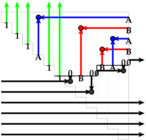
Figure 5. The rays and dots of a slice. This example has no $1$-dot, because the East edge of the kink is not $\,\big{|}\!\!\!1$.

So in the absence of $K$-labels, the above arrangement of dots is our definition of the partial permutation associated to the slice $s$. We will denote this $g(s)$, later to avoid confusion with the $f(P)$ associated to an IP pipe dream.

If one extends $f$ to a bounded juggling pattern $J$, by placing dots Northwest/Southeast in the missing rows and columns, then the $0$- and $1$-rays that continue outside the triangle can be imagined as pointing at these other dots.

4.1.2. With $K$-labels

So far the rays described have only one label, and two rays either cross unimpeded if they have different labels, or mutually annihilate (leaving a dot) if they have the same label.

What changes now is that there is one slice edge that can have more than one label: the East edge of the kink, labeled $V\not\ni 0$. We give this West-pointing ray the special property that if it crosses a North-pointing ray with (just one) label $c$, then

• if $c$ is not in $V$, and $V$ doesn’t end with $1$, the rays cross unimpeded

• if $c$ is not in $V$, and $V$ ends with $1$, $c$ must be $0$ and the rays cross unimpeded

• if $V$ ends with $c$, then the rays cross through each other but both change as depicted in the displacer tile; in particular the West-pointing ray loses its terminal letter ($c$)

• if $c$ is in $V$, but is not its last letter, then $s$ is not viable.

To check viability, then, we continue this West-pointing ray, successively losing its terminal letters where it doesn’t cross disjointly-labeled rays, until it gets down to a single label. At that point we have reduced to the previous definition of viability.

Proposition 4.1.

Let $s$ be a viable slice, with kink at $(i,j)$, and $f$ its associated partial permutation. Then $\textcyr{X}_{i\to j}$ is a safe shift for $\Pi_{f}$.

The East and South edges of the kink are both labeled $0$ iff $(i+1,j)$ is an essential box for $f$. Otherwise, $\Pi_{f}$ is $\textcyr{X}_{i\to j}$-invariant.

Proof.

The $i=j$ case is silly and we dispense with it first. Of course the shift is safe, $\Pi_{f}$ is $\textcyr{X}_{i\to i}$-invariant, and the South edge is labeled $1$, not $0$.

Now, let $(a,b)$ be an essential box in $f$’s diagram, with $i<a\leq j\leq b$; we need to show that $(a,b)=(i+1,j)$.

Since $a\geq i+1$, the box $(a,b)$ is in the “bottom half”, where there are only $0$-dots. Since $(a,b)$ is not crossed out from the East (meaning, in $f$’s diagram – not by a ray, in this context!) there is a $0$-dot to its West. Assume for contradiction that $a>i+1$. Then there is also a $0$-dot in the row above, further West. Since $(a,b)$ is not crossed out from above, neither is the box $(a-1,b)$ above it. So if $a>i+1$, then $(a-1,b)$ is not crossed out at all, making $(a,b)$ inessential. Contradiction; hence $a=i+1$.

Since $(a=i+1,b)$ is not crossed out from above, neither is $(i,b)$, so it must be crossed out from the East (or else $(i+1,b)$ wouldn’t be essential). Hence the East edge of the kink must be $\,\big{|}\!\!\!0$, and the ray coming East out of this $\,\big{|}\!\!\!0$ must pass all the way through the $(i,b)$ box.

If $b>j$, then since $(i,b)$ is not crossed out from above, the slice label atop the $(i,b)$ square must be $-\!\!\!-\!\!\!\!\!\!0\$. So the ray just mentioned would stop in the $(i,b)$ square, not pass through, contradiction. Hence $j=b$, concluding the proof that the shift is safe.

Say $(i+1,j)$ is essential. Then since it is not crossed out from above, the slice label South of the kink must be $-\!\!\!-\!\!\!\!\!\!0\$. Since the box above must be crossed out from the East, the slice label East of the kink must also be $\,\big{|}\!\!\!0$.

Now the converse. If the East edge of the kink is $\,\big{|}\!\!\!0$, then $(i,j)$ is not in the diagram (either the row’s dot is to the right, or there is no dot). If the South edge of the kink is $-\!\!\!-\!\!\!\!\!\!0\$, then $(i+1,j)$ is not crossed out from the North or East, and is in the diagram. For $(i+1,j)$ to be essential, though, we still need that $(i+1,j+1)$ is crossed out, and there are two cases to consider. If the slice label above $(i,j+1)$ is $-\!\!\!-\!\!\!\!\!\!0\$, then there is a $0$-dot at $(i,j+1)$. Otherwise there is a ray upward from this slice label, and $(i,j+1)$ is crossed out from above. Either way $(i+1,j+1)$ is crossed out from above. This shows that if both labels are $0$, then $(i+1,j)$ is an essential box for $f$. ∎

4.2. The West edges are automatically $0$s

Proposition 4.2.

Let $P$ satisfy all the requirements of a $K$-IP pipe dream except for the condition that the West edge labels are $0$s. Then this condition holds iff the number of letters on the South edges equals that on the East edges.

Proof.

If a West edge label of a tile contains a $1$, then the tile can’t be a displacer (since the $Wbc$ on the East edge wouldn’t end with $1$), so the South edge must be $0$. This can’t happen on a tile at $(i,i)$, so none of the West edges of the pipe dream contain $1$s.

If a $1$-pipe enters a fusor tile from the West, it must come out the North. So the $1$-pipes go from South edges of the $K$-IP pipe dream to North edges.

Denote the numbers of labels on the North edge by $N_{0}+N_{1}=n$, where $N_{0},N_{1}$ are the numbers of labels $0,1$, on the East edge by $E_{0}+E_{L}=n$ (with $L$ for Letter), and on the South edge by $S_{1}+S_{L}=n$. Then so far we have argued $S_{1}=N_{1}$. From the North, the number of $0$-pipes coming out the West is $n-N_{1}=n-S_{1}=S_{L}$. From the East, the number is $n-E_{L}$. Summing, we get $n-E_{L}+S_{L}$ $0$-pipes on the West, so every West edge ends with $0$ iff $S_{L}=E_{L}$. ∎

4.3. Placing the next tile

Let $s$ be a viable slice, with kink at $(i,j)$. Say that $s$ admits a tile $\tau$, producing the slice $s^{\prime}$, if

• the upper half of $s$ has one more box (namely, the kink) than the upper half of $s^{\prime}$,

• if $s,s^{\prime}$ agree on all common edges,

• the edges on which they differ bound the tile $\tau$ (at $(i,j)$), and

• $s^{\prime}$ is again viable.

Proposition 4.3.

Let $s$ be a viable slice such that the East and South edges of the kink are not both labeled $0$. Then $s$ admits a unique tile, and the $s^{\prime}$ produced has the same associated partial permutation as $s$ did.

Proof.

This is a straightforward case check, which we recommend to the reader. Spoilers commence for those who resist the pleasure.

If the East and South edge of the kink have disjoint labels, then the tile $\tau$ must be a crossing tile. The rays from the new horizontal and vertical edges are labeled and pointing the same directions as before. They match up with (or otherwise modify) the same perpendicular rays as they did before.

If these edges have the same label $b\neq 0$, then in the partial permutation associated to $s$, there is a $b$ dot inside the kink. The tile $\tau$ must be a “dot” tile (in the list from §1.5.1). When we fill it in, the slice $s^{\prime}$ so produced has a $0$ dot in the same place.

Otherwise the East edge must have multiple labels on it. By the definition of viability from §4.1.2, the South label must be the last letter of the East label, and filling in the displacer tile to create $s^{\prime}$ both preserves viability, and leaves the dots in place. (This is of course due to our recursive definition of viability, in the presence of multiple labels.)

∎

The remaining case – when the East and South edges of the kink are both labeled $0$ – is much more interesting.

Proposition 4.4.

Let $s$ be a viable slice, with kink at $(i,j)$, whose South and East edges are labeled $0$. (In particular $i<j$, since there are no South $-\!\!\!-\!\!\!\!\!\!0\$ labels on $(i,i)$ tiles.) So $s$ admits only fusor tiles.

One such that $s$ admits is the equivariant tile, and the $s^{\prime}$ so produced has $\Pi_{f(s^{\prime})}=\Psi_{i\to j}\Pi_{f(s)}$.

The dots in $f(s)$ that are minimally Northwest of $(i,j)$, and in columns $[i,j]$, have all distinct labels. Let $C$ be the list of these labels (read SW to NE), plus $1$ at the end if the $s$-labels West of the kink end $1\ 0^{m}$.

For each nonempty sublist $S\subseteq C$, $s$ admits the fusor tile with West edge $S$. These tiles (and the equivariant tile) are all the tiles $s$ admits, and for each such $S$ the resulting $s^{\prime}$ has $\Pi_{f(s^{\prime})}=\bigcap_{i^{\prime}\in S}\Pi_{f(s)\circ(i\leftrightarrow j)\circ(i^{\prime}\leftrightarrow i)}$ as last seen in theorem 3.15.

Proof.

Before placing the equivariant tile, there are $0$-rays coming South and East out of the kink. The South-pointing ray goes down to a $0$-dot $\delta$, and the East-pointing ray either meets a South-pointing $0$-ray $\rho$ at a $0$-dot, or it exits the bottom half entirely. Once we place the equivariant tile at the kink, producing $s^{\prime}$, the $0$-rays each start one step back, and now collide at a $0$-dot in $(i,j)$. If there is a $\rho$, it no longer hits the East-pointing $0$-ray from the kink, but continues down to the row where $\delta$ was. Effectively, $\delta$ has moved up into $(i,j)$, and the $0$-dot from row $i$ (if there is one) has moved down to $\delta$’s row. This is exactly the sweeping action on dots computed in proposition 3.13. The fact that the ray/dot picture continues to exist is our definition of viability.

Since two dots in $f(s)$ with the same label were required to be NW/SE of each other, the dots that are minimally Northwest of $(i,j)$ must have distinct labels. Let $C$ be the list of those dots in columns $[i,j]$ (read SW to NE), plus $1$ at the end if the $s$-labels west of the kink end $1\ 0^{m}$. We now claim that $s$ admits a fusor tile with West edge $W$ $\Longleftrightarrow$ the list $W$ is a (nonempty) sublist of $C$.

For each direction of this iff, it helps to understand what tiles will be placed after (i.e. further left from) the fusor is placed. There are only crossings (which copy the vertical labels) and displacers (which remove one letter from $W$ at a time, from the right), until all the letters in $W$ are gone and we hit a dot tile. (More tiles are forced thereafter, usually, but this is enough to consider.) We have to hit a dot tile at some point, because by proposition 4.2 the leftmost vertical edge will be a $\,\big{|}\!\!\!0$. See figure 6 for the full story.

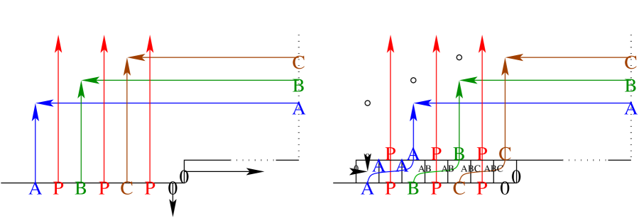
Figure 6. From the left to the right figure, we place the fusor tile, forcing the next several displacer and crossing tiles, then the dot tile. The little circles in the right figure show where the dots were, before they moved rightward. Hopefully this picture also indicates the motivation of the name “displacer” tile.

$\Longleftarrow$ Place the tile, producing $s^{\prime}$, and the follow-on tiles up through the first dot tile. To show this preserves viability, we have to show that there is again a consistent system of rays and dots; this is best illustrated in figure 6.

$\Longrightarrow$ We claim that if $s$ admits a fusor tile with West edge $W$, then $W$ must be a sublist of $C$. Each displacer tile encountered before the dot tile lies over a letter or a $1$, with a North-pointing ray. We claim that the dot that ray points to (interpreting the ray from a $-\!\!\!-\!\!\!\!\!\!\!\!1\$ as pointing to a dot just outside the triangle) is minimally Northwest of $(i,j)$.

This is easy for the $-\!\!\!-\!\!\!\!\!\!\!\!1\$ case. By the condition on crossing tiles, before we meet the $-\!\!\!-\!\!\!\!\!\!\!\!1\$ displacer we go through $-\!\!\!-\!\!\!\!\!\!0\$ crossing tiles, whose dots are to the South.

Otherwise the displacer tile at $(i,j^{\prime})$ lies atop a letter, say $A$, with a ray pointing up to an $A$-dot. If the $A$-dot is not minimally Northwest of $(i,j)$, then there is another (say) $B$-dot in some column $j^{\prime\prime}$, $j^{\prime}<j^{\prime\prime}<j$ in between the $A$-dot and $(i,j)$. (So $B$ is a letter, not $0$ or $1$.) We do assume this $B$-dot to be minimally Northwest, so, lying atop the rightmost $-\!\!\!-\!\!\!\!\!\!\!\!B\$ left of $(i,j)$. This letter $B$ must be distinct from $A$, or else the $A$ would already have been ripped out of the vertical label. Before we place the fusor tile, the $A$-rays and $B$-rays do not intersect at all, by the $B$-dot being SE of the $A$-dot.

There are two cases: the fusor tile involves the label $B$, or not.

If not, then once we place tiles at $(i,j)$–$(i,j^{\prime})$, going from the left figure here to the right figure,

the $A$-pipe crosses the $B$-pipe once in the tiles and once in the rays. Placing more tiles won’t fix the latter intersection, by the Jordan curve theorem, so we know that whatever pipe dream we make eventually will have two lettered pipes crossing twice. That being forbidden is the contradiction that says there is no offending $B$-dot.

If yes, then the West label of the fusor tile involves both $A$ and $B$ so we are definitely using $K$-pieces. Now we invoke the nonlocal condition on $K$-IP pipe dreams (look again at §1.5.1) and Jordan curve to reach a similar contradiction. ∎

4.4. Proofs of the main theorems

Proof of theorem 1.4.

This just combines propositions 4.1, 4.3, and 4.4. ∎

The other proofs are by induction through the Vakil sequence. For each pair $(i\leq j)$, define a $K$-IP pipe dream $P$ below $(i,j)$ to be a viable slice at $(i,j)$ plus a filling of its bottom half with $K$-tiles. We can interpret the previous definition of $K$-IP pipe dream as the $(i=0,j=n)$ case, and otherwise require $i\in[n]$. (These partial pipe dreams will be directly useful in [KnLed].)

It is clear how to extend the definition of $f(P)$, $fusing(P)$, and $wt_{K}(P)$ to these partial pipe dreams. And since each comes with a slice, we can define the partial permutation $g(P)$ to be $g($that slice$)$. For $(i,j)=(n,n)$ (no tiles) we have $g(P)=f(P)$, whereas for $(i,j)=(0,n)$ (usual $K$-IP pipe dreams), we have $g(P)$ running NW/SE, in the first $n-k$ rows, with columns determined by $\lambda(P)$.

Proof of theorems 1.6, 1.5, 1.2, 1.1.

We will prove first a generalization of theorem 1.6, that for each $(i\leq j)$,

$$[\Pi_{f}]=\sum_{P:\ f(P)=f}(-1)^{fusing(P)}wt_{K}(P)\ [\Pi_{g(P)}]$$

where the $P$ summed over are the $K$-IP pipe dreams below $(i,j)$. When $(i,j)=(0,n)$, this is just the sum over $K$-IP pipe dreams $P$, and $\Pi_{g(P)}=X^{\lambda(P)}$ by lemma 2.2.

The proof will be by induction through the Vakil order, where the base case is $(i,j)=(n,n)$, handled by lemma 2.3. There is a unique (tile-less) $K$-IP pipe dream $P$ below $(n,n)$, and $g(P)=f(P)=f$, giving the equation $[\Pi_{f}]=(-1)^{0}\cdot 1\cdot[\Pi_{f}]$. In the inductive step, we want to place one tile on each $P$ in the summation.

If the South and East edges of the kink are not both labeled $0$, then $\Pi_{g(P)}$ is $\textcyr{X}_{i\to j}$-invariant (proposition 4.1), and there is a unique way of placing the tile and it does not move the dots (proposition 4.3).

If the South and East edges of the kink are both labeled $0$, let $P_{e}$ be $P$ plus an equivariant piece, and $\{P_{S}\}_{S\subseteq C},S\neq\emptyset$, where $C$ is as in proposition 4.4.

Since positroid varieties are $T$-convex by theorem 3.10 (1 or 2), we can use the degree $1$ result from theorem 3.10 (3). That, and them having rational singularities justifies use of proposition 3.5 which computes $K_{T}$-classes using shifts. It says

$$[\Pi_{g(P)}] = (1-\exp(y_{j}-y_{i}))[\Psi_{i\to j}\Pi_{g(P)}]+\exp(y_{j}-y_{i})[\textcyr{X}_{i\to j}\Pi_{g(P)}]$$

$$= (1-\exp(y_{j}-y_{i}))[\Pi_{g(P_{e})}]+\exp(y_{j}-y_{i})\sum_{S\subseteq C,\ S\neq\emptyset}(-1)^{\#S-1}[\Pi_{g(P_{S})}]$$

by proposition 4.4 and theorem 3.15, which we rewrite as

$$= \sum_{P\text{ admits }\tau}(-1)^{fusing(\tau)}wt_{K}(\tau)[\Pi_{g(P\&\tau)}].$$

If we use that recursively, and the multiplicativity of the definition of $fusing$ and $wt_{K}$, we get the generalization claimed.

This directly implies theorem 1.5 by taking all $y_{i}=0$, and from there theorem 1.1 by taking leading terms.

With some care we could derive the $H^{*}_{T}$ theorem 1.2 as the leading terms of this $K_{T}$ formula. But it is simpler just to replace the use of proposition 3.5’s $K_{T}$-formula with its $H^{*}_{T}$-formula. From that point the derivation is the same.

Finally, we address the fusing count from the end of theorem 1.5, proving by induction more generally that

$$fusing(P)=\dim\Pi_{f(P)}-\dim\Pi_{g(P)}+\#\text{equivariant tiles}$$

for these partial pipe dreams. The base case of the induction is $P$ empty, where $f(P)=g(P)$. For the induction, we see how $g(P)$ changes as we attach one tile, using the analyses of propositions 4.3 and 4.4. There are three cases:

1. Unique fill. See proposition 4.3. We don’t change $fusing(P)$ or $g(P)$, nor attach an equivariant tile, so none of the four numbers change.

2. Equivariant tile. See proposition 4.4. We change $g(P)$ by a covering relation in affine Bruhat order, increasing $\dim\Pi_{g(P)}$ and the number of equivariant tiles each by $1$.

3. Fusing. See proposition 4.4. The change in length of $g(P)$ matches the change in the fusing number.

∎

5. Puzzles $\quad\leftrightarrow\quad$ IP pipe dreams with one letter

In this section we consider IP pipe dreams (not $K$-IP) with only one letter, i.e. the edge labels are $\{0,1,R\}$. This has two interesting effects.

The first is that in the initial (and every later) slice $s$ the dots in the top half of $f(s)$ are NW/SE, and consequently, the interval positroid variety associated to an initial slice (where the top half is the whole upper triangle) is a Richardson variety $X_{\mu}\cap X^{\nu}$. In particular, its homology class is given by the Littlewood-Richardson rule, and its geometric shifts have already been studied in [Va06].

The second effect is that the conditions defining the IP (but not $K$-IP) pipe dreams become entirely local: since two lettered pipes with the same letter don’t cross even once, they definitely won’t cross twice, and there aren’t two different letters to worry about.

5.1. Puzzles

We give a slightly modified definition of the equivariant puzzles from [KnTao03]. The puzzle labels are $0$, $1$, $R$, and the puzzle pieces are these:

A size $n$ puzzle is a tiling of a size $n$ equilateral triangle (parallel to those above) with puzzle pieces, such that the boundary has no $R$ labels. Consequently, the pieces with $R$s come in adjacent pairs, the $R$ being for “rhombus”. The fourth piece is the equivariant piece, with equivariant weight $y_{i}-y_{j}$, where $i$ is the distance of that piece from the Northwest side of the puzzle, and $n-j$ its distance from the Northeast side. (Other pieces have equivariant weight $1$.)

To compare puzzles to IP pipe dreams, it is mnemonic to first compare the equivariant rhombus of weight $y_{i}-y_{j}$ to the corresponding equivariant tile. We will need to stretch the puzzle to drape each rhombus across the corresponding square, and will need to change the labels on vertical edges.

Theorem 5.1.

Given a puzzle of size $n$, apply the following transformations:

1. Move the North corner right until it is above the Southeast corner, then the Southwest corner up until it is left of the North corner.

2. Along the NW/SE diagonal, attach and pieces so that the resulting shape is that of an IP pipe dream.

3. Erase all diagonal labels, so the result is a bunch of labeled squares.

4. On vertical edges, rotate the labeling $\,\big{|}\!\!\!R\mapsto\,\big{|}\!\!\!1\mapsto\,\big{|}\!\!\!0\mapsto\,\big{|}\!\!\!R$. Horizontal labels we leave alone.

Then the result is an IP pipe dream. An example is in figure 7.

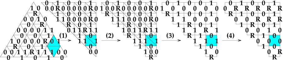
Figure 7. The transformation of a puzzle, weight $y_{4}-y_{5}$, into an IP pipe dream.

Let $\lambda,\mu,\nu\in{[n]\choose k}$. This composite transformation gives a weight-preserving bijection between

• puzzles with $\lambda,\mu,\nu$ giving the positions of the $1$s on the NW, NE, and S sides (each read left-to-right), and

• IP pipe dreams with only the labels $\{0,1,R\}$, where $\lambda$ gives the positions of the $1$s on the North side, and $\mu,\nu$ give the positions of the $R$s on the East side (read top-to-bottom) and South side (read left-to-right).

Proof.

Since both definitions are local, the proof is simply a correspondence between the $9$ ways to attach two triangles together ($1$ with $R$ on the diagonal, $2*2*2$ if one chooses the diagonal to be $0,1$ and then chooses each half), plus the equivariant rhombus, to the $10$ possible tiles ($2$ dot tiles, $2$ fusors, $3*2-1$ crossing, $1$ equivariant). Here it is:

∎

Since we are working in equivariant cohomology and not $K$-theory, the Schubert and opposite Schubert bases are dual bases in the sense that $\int_{Gr_{k}({\mathbb{A}}^{n})}[X_{\lambda}][X^{\mu}]=\delta_{\lambda\mu}$. So instead of interpreting puzzles as computing the coefficient of $[X^{\lambda}]$ in the class $[X_{\mu}\cap X^{\nu}]=[X_{\mu}][X^{\nu}]$ of the Richardson variety, we can equivalently interpret them as computing the coefficient of $[X_{\nu}]$ in the product $[X_{\lambda}][X_{\mu}]$, giving the main result of [KnTao03].

One benefit of the puzzle combinatorics over that of the IP pipe dreams is to make combinatorially evident a $\mathbb{Z}/3$-symmetry of the nonequivariant Schubert structure constants, namely $c_{\lambda\mu}^{\nu^{*}}=c_{\mu\nu}^{\lambda^{*}}$, since both equal $\int_{Gr_{k}({\mathbb{A}}^{n})}[X_{\lambda}][X_{\mu}][X_{\nu}]$. (This symmetry does not hold equivariantly, since the dual basis element $[X^{\lambda}]$ to $[X_{\lambda}]$ only equals $[X_{\lambda^{*}}]$ nonequivariantly. And sure enough, the puzzle rule is only rotationally symmetric when we exclude the equivariant piece.)

The paper [ZJ09] also reinterprets puzzles in terms of pipes, or more properly space-time diagrams of two colors of fermions moving on a line, but the world-lines of those particles don’t seem to have much to do with the pipes here.

References

- [ABS] Sami Assaf, Nantel Bergeron, Frank Sottile: Multiplying Schubert polynomials by Schur functions, in preparation.
- [AGriMil11] David Anderson, Stephen Griffeth, Ezra Miller: Positivity and Kleiman transversality in equivariant -theory of homogeneous spaces. J. European Math Society 13 (2011), 57–84. http://arxiv.org/abs/0808.2785
- [B76] Andrzej Białynicki-Birula: Some properties of the decompositions of algebraic varieties determined by actions of a torus. Bull. Acad. Polon. Sci. Sér. Sci. Math. Astronom. Phys. 24 (1976), no. 9, 667–674.
- [BiCo12] Sara Billey, Izzet Co skun: Singularities of generalized Richardson varieties. Communications in Algebra. 40:4 (2012), 1466–1495. http://arxiv.org/abs/1008.2785
- [BdM08] Joseph Bonin, Anna de Mier: The lattice of cyclic flats of a matroid. Ann. Comb. 12 (2008), no. 2, 155–170. http://arxiv.org/abs/math/0505689
- [BGW03] Alexandre Borovik, Israel Gelfand, Neil White: Coxeter matroids. Progress in Mathematics 216, Birkhäuser.
- [Bri02] Michel Brion: Positivity in the Grothendieck group of complex flag varieties, J. Algebra (special volume in honor of Claudio Procesi) 258 (2002), 137–159. http://arxiv.org/abs/math/0105254
- [EKR61] Pál Erdős, Chao Ko, Richard Rado: Intersection theorems for systems of finite sets, Quarterly Journal of Mathematics, Oxford Series, series 2 (1961) 12: 313–320. http://dx.doi.org/10.1093/qmath/12.1.313
- [FoS] Nicolas Ford, David Speyer: in preparation.
- [Fr87] Peter Frankl: The shifting technique in extremal set theory. Surveys in combinatorics 1987 (New Cross, 1987), 81–110, London Math. Soc. Lecture Note Ser., 123, Cambridge Univ. Press, Cambridge, 1987.
- [Fu92] William Fulton: Flags, Schubert polynomials, degeneracy loci, and determinantal formulas, Duke Math. J. 65 (1992), no. 3, 381–420.
- [Gr00] William Graham: Positivity in equivariant Schubert calculus, Duke Math. J. 109 (2001), no. 3, 599–614. http://arxiv.org/abs/math.AG/9908172
- [HL] Xuhua He, Thomas Lam: Projected Richardson varieties and affine Schubert varieties, preprint. http://arxiv.org/abs/1106.2586
- [Ka02] Gil Kalai: Algebraic shifting. Computational commutative algebra and combinatorics (Osaka, 1999), 121–163, Adv. Stud. Pure Math., 33, Math. Soc. Japan, Tokyo, 2002.
-
[KnMY09]
Allen Knutson, Ezra Miller, Alex Yong:
Gröbner geometry of vertex decompositions and of flagged tableaux.
J. Reine Angew. Math. 630 (2009), 1–31.
http://arxiv.org/abs/math/0502144 - [KnTao03] by same author, Terence Tao: Puzzles and (equivariant) cohomology of Grassmannians, Duke Math. J. 119 (2003), no. 2, 221–260. http://arxiv.org/abs/math.AT/0112150
- [K] by same author: Puzzles, positroid varieties, and equivariant -theory of Grassmannians, unpublished. http://arxiv.org/abs/1008.4302
- [KLS13] by same author, T. Lam, D. Speyer: Positroid varieties: juggling and geometry, Compositio Mathematica, Volume 149, Issue 10, October 2013, pp 1710–1752. http://arxiv.org/abs/1111.3660
- [KLS14] by same author, Thomas Lam, David Speyer: Projections of Richardson varieties, Journal für die reine und angewandte Mathematik (Crelle’s Journal) 2014.687 (2014): 133–157. http://arxiv.org/abs/1008.3939
- [KnLed] by same author, Mathias Lederer: A -deformation of the ring of symmetric functions, in preparation.
- [LS07] Thomas Lam, Mark Shimozono: A Little bijection for affine Stanley symmetric functions. Sém. Lothar. Combin. 54A (2005/07), Art. B54Ai, 12 pp. http://arxiv.org/abs/math/0601483
-
[MPP]
Karóla Mészáros, Greta Panova, Alex Postnikov:
Schur times Schubert via the Fomin-Kirillov algebra,
Electronic J. Combinatorics, Vol 21, Issue 1 (2014).
http://arxiv.org/abs/1210.1295 -
[Pos]
Alex Postnikov:
Total positivity, Grassmannians, and networks, preprint.
http://www-math.mit.edu/~apost/papers/tpgrass.pdf - [Va06] Ravi Vakil: A geometric Littlewood-Richardson rule, Annals of Math. 164 (2006), 371–422. http://annals.math.princeton.edu/annals/2006/164-2/p01.xhtml
- [W75] Neil White: The bracket ring of a combinatorial geometry. I. Trans. Amer. Math. Soc. 202 (1975), 79–95.
- [ZJ09] Paul Zinn-Justin: Littlewood-Richardson coefficients and integrable tilings. Electron. J. Combin. 16 (2009), Research Paper 12. http://arxiv.org/abs/0809.2392