Communication strength of correlations violating monogamy relations

Abstract

In any theory satisfying the no-signaling principle correlations generated among spatially separated parties in a Bell-type experiment are subject to certain constraints known as monogamy relations. Recently, in the context of the black hole information loss problem it was suggested that these monogamy relations might be violated. This in turn implies that correlations arising in such a scenario must violate the no-signaling principle and hence can be used to send classical information between parties. Here, we study the amount of information that can be sent using such correlations. To this aim, we first provide a framework associating them with classical channels whose capacities are then used to quantify the usefulness of these correlations in sending information. Finally, we determine the minimal amount of information that can be sent using signaling correlations violating the monogamy relation associated to the chained Bell inequalities.

1 Introduction

In recent years a lot of research has been devoted to probabilistic nonsignaling theories GNT ; GNT2 . They are formulated in terms of boxes, that is, families of probability distributions describing correlations generated in a Bell-type experiment by spatially separated observers. The boxes are required to satisfy the no-signaling principle which means that expectation values seen by some of the observers cannot depend on the measurement choices made by the remaining ones (see e.g. Ref. review ). A particular example of a theory obeying the no-signaling principle is quantum mechanics. It was realized, however, that there exist nonsignaling theories which lead to higher violations of Bell inequalities than it is allowed by quantum mechanics PR . This discovery raised a debate as to whether such supra-quantum nonsignaling correlations can be found in Nature (see, e.g., Refs. principles ).

One of the most interesting features of the nonsignaling correlations is that they are monogamous Toner ; Marcin ; monog ; Ravi . Consider for instance a three-partite scenario in which Alice and Bob violate the Clauser-Horne-Shimony-Holt (CHSH) CHSH or the chained BC90 Bell inequality up to its maximal algebraic value. Then, each of Alice’s or Bob’s observables appearing in it cannot be correlated with an arbitrary observable measured by Eve monog . This fact found important applications in cryptography based on nonsignaling principle KD and randomness amplification RA —tasks that are impossible in classical world.

Although all well-established physical theories satisfy the no-signaling principle, there is at least one important physical phenomenon where monogamy relations can be violated—the black hole information loss problem. It was argued by Almheiri, Marolf, Polchinski, and Sully that if information escapes from black hole, then one can check if the entanglement monogamy is violated (Almheiri, , page 5). Later, Oppenheim and Unruh showed that by performing measurements on three particles in a “polygamous entangled state” near black hole, one can send superluminal signals, thus giving rise to a box violating the no-signaling principle. Let us also note that if one allows for post-selection in the Bell-type experiment, violation of monogamy relations can appear in quantum mechanics Preskill , which can have applications to black hole information loss problem Horowitz .

Let us now consider a box violating a monogamy relation. Then, this box must be signaling. Then, the natural question appears: how can the box be used to send information from some parties to the other parties, and, moreover, how much communication can be sent? In this Letter we answer these questions for three-partite boxes which violate monogamy relations for the CHSH and the chained Bell inequalities. We also present a very simple proof of the monogamy relations introduced in Ref. monog . By putting monogamy relations in a broader framework allows one to get a better understanding of their structure.

Before presenting our results, we need to introduce some notation and terminology. Imagine that three parties $A$, $B$, and $E$ perform a Bell-type experiment in which $A$ and $B$ can measure one of $M$ observables, denoted $A_{i}$ and $B_{j}$, respectively, while the external observer $E$ measures a single observable, which we also denote by $E$. We assume that all these observables have two outcomes $\pm 1$, denoted $a$, $b$, and $e$. The correlations that are generated in such an experiment are described by a set of probabilities $\{p(A_{i}B_{j}E)\equiv p(a,b,e|A_{i},B_{j})\}$, where $p(a,b,e|A_{i},B_{j})$ is the probability of obtaining $a,b,e$ when $A_{i}$, $B_{j}$ and $E$ have been measured by $A$, $B$, and $E$, respectively. In what follows we arrange these probabilities in vectors denoted $\vec{p}$ and refer to them as boxes. We then say that the distribution $\{p(A_{i}B_{j}E)\}$ obeys the no-signaling principle (it is nonsignaling) if all of its marginals describing a subset of parties is independent of the measurement choices made by the remaining parties, i.e.,

$$\sum_{a}p(a,b,e|A_{i}B_{j}) = \sum_{a}p(a,b,e|A_{k}B_{j}),$$ (1)

and

$$\sum_{b}p(a,b,e|A_{i}B_{j}) = \sum_{b}p(a,b,e|A_{i}B_{k}),$$ (2)

are satisfied for any triple $i,j,k$. Then, by $\langle XY\rangle_{Z}$ we denote the standard bipartite expectation value of the product of observables $X$ and $Y$, which in general might be conditioned on the third party’s measurement choice $Z$. An example of such conditional expectation value is

$$\langle A_{i}E\rangle_{B_{j}}=\sum_{a,b,e=\pm 1}a\cdot e\cdot p(a,b,e|A_{i},B_{j}).$$ (3)

If $\{p(a,b,e|A_{i},B_{j})\}$ is nonsignaling, then clearly $\langle XY\rangle_{Z}=\langle XY\rangle_{Z^{\prime}}\equiv\langle XY\rangle$ for any choice of $X$, $Y$, and $Z\neq Z^{\prime}$.

Let us finish the introductory section be defining what we mean by ”classical information” in the Bell-type scenario introduced above. In this scenario, the parties have access only to measurements of classical random variables associated to observables $A_{i}$, $B_{j}$ and $E$. In this sense the results of the experiments are inherently classical and carry the classical information to which we refer in latter parts of the paper. For instance, if $A$ decides to measure the observable $A_{i}$, its result is either $-1$ or $1$ and thus can be encoded in one logical bit. Analogously, a result of the joint measurement of the observables $A_{i}$,$B_{j}$ and $E$ is can be encoded in tree logical bits.

2 A simple derivation of a monogamy relation for the CHSH Bell inequality

For clarity we begin our considerations with the simplest scenario of $M=2$.

The key ingredient of our framework is a simple proof of the monogamy relation obeyed by any nonsignaling probability distribution $\{p(a,b,e|A_{i},B_{j})\}$ Toner ; monog :

$$|I_{AB}|+2|\langle B_{0}E\rangle|\leq 4,$$ (4)

where $I_{AB}$ stands for the Bell expression giving rise to the well-known CHSH Bell inequality CHSH

$$I_{AB}:=\langle A_{0}B_{0}\rangle+\langle A_{1}B_{0}\rangle+\langle A_{1}B_{1}\rangle-\langle A_{0}B_{1}\rangle\leq 2.$$ (5)

The inequality (4) compares the nonlocality shared by $A$ and $B$, as measured by the violation of (5), to the (classical) correlations that the external party $E$ can establish with the outcomes of $B_{0}$. It should be noticed that it remains valid if in the last correlator, $B_{0}$ is replaced by any $A_{i}$ or $B_{i}$ (for clarity, however, we proceed with a fixed measurement $B_{0}$). Also, without any loss of generality we can assume that both $I_{AB}$ and $\langle B_{0}E\rangle$ are positive; if this is not the case, we redefine observables $A_{0}$, $A_{1}$ and/or $E$ in the following way: $A_{0}\rightarrow-A_{0}$, $A_{1}\rightarrow-A_{1}$, and/or $E\rightarrow-E$. Consequently, in what follows we omit the absolute values in (4).

In order to prove (4), let us first make the following observation. Suppose that for some random variables $X$, $Y$ and $Z$ taking values $\pm 1$ there exists the joint probability distribution $p(XYZ)$. Then, the latter fulfils the following inequalities

$$(-1)^{i}\langle XY\rangle_{Z}+(-1)^{j}\langle YZ\rangle_{X}+(-1)^{k}\langle XZ\rangle_{Y}\leq 1,$$ (6)

with $i,j,k=0,1$ such that $i\oplus j\oplus k=1$, where addition is modulo 2. To prove (6), it suffices to check it for the extremal values of correlators.

Now, one notices that each triple of observables $A_{i}$, $B_{j}$ and $E$ is jointly measurable and therefore, for any pair $i,j$, there exists the joint probability distribution $p(A_{i}B_{j}E)$ which must satisfy (6). This gives rise to the following four inequalities

$$\langle A_{0}B_{0}\rangle_{E}+\langle B_{0}E\rangle_{A_{0}}-\langle A_{0}E\rangle_{B_{0}} \leq 1,$$ (7)

$$\langle A_{1}B_{0}\rangle_{E}+\langle B_{0}E\rangle_{A_{1}}-\langle A_{1}E\rangle_{B_{0}} \leq 1,$$ (8)

$$\langle A_{1}B_{1}\rangle_{E}-\langle B_{1}E\rangle_{A_{1}}+\langle A_{1}E\rangle_{B_{1}} \leq 1,$$ (9)

$$-\langle A_{0}B_{1}\rangle_{E}+\langle B_{1}E\rangle_{A_{0}}+\langle A_{0}E\rangle_{B_{1}} \leq 1.$$ (10)

By summing these up and using the fact that in a nonsignaling theory $\langle XY\rangle_{Z}=\langle XY\rangle_{Z^{\prime}}$ for any $Z\neq Z^{\prime}$, one obtains (4).

3 Signaling boxes as classical channels

Let us assume that correlators $\langle B_{0}E\rangle_{A_{0}}$ and $\langle B_{0}E\rangle_{A_{1}}$ are equal (later we will show how this assumption can be relaxed). Then the monogamy relation (4) is well defined. It bounds the possible correlations achievable in any no-signaling theory between outcomes of measurements performed by the three parties $A$, $B$ and $E$. If it is violated by some probability distribution $\vec{p}$, then the latter must violate the no-signalling principle, in which case we call such a box signaling. In other words, if $\vec{p}$ violates (4), then values of some bipartite correlators become dependent on the measurement choice made by the third party. This dependence allows one to use such signaling boxes to send information from a single party to the remaining two parties. To illustrate this idea, suppose that a box $\vec{p}$ violates the relation (4) by $\Delta>0$, that is,

$$R(\vec{p})\equiv I_{AB}+2\langle B_{0}E\rangle=4+\Delta.$$ (11)

Then, by adding the inequalities (7)-(10), one concludes that

$$\langle A_{0}E\rangle_{B_{0}}-\langle A_{0}E\rangle_{B_{1}}+\langle A_{1}E\rangle_{B_{0}}-\langle A_{1}E\rangle_{B_{1}}+\langle B_{1}E\rangle_{A_{1}}-\langle B_{1}E\rangle_{A_{0}}\geq\Delta.$$ (12)

Consequently, in at least one of the three pairs

$$S_{B\to AE}^{0} = \{\langle A_{0}E\rangle_{B_{0}},\langle A_{0}E\rangle_{B_{1}}\},$$ (13)

$$S_{B\to AE}^{1} = \{\langle A_{1}E\rangle_{B_{0}},\langle A_{1}E\rangle_{B_{1}}\},$$ (14)

$$S_{A\to BE}^{1} = \{\langle B_{1}E\rangle_{A_{1}},\langle B_{1}E\rangle_{A_{0}}\},$$ (15)

the correlators must differ. In particular, in one of them the difference must not be lower than $\Delta/3$. The correlators in $S_{B\to AE}^{i}$ correspond to signaling from $B$ to the pair $A$ and $E$, while those in $S_{A\to BE}^{i}$ to signaling from $A$ to $B$ and $E$.

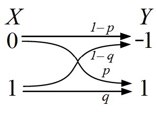
Figure 1: A binary classical channel that can be associated to one of the pair of correlators $S^{i}_{A\to BE}$ and $S^{i}_{B\to AE}$ with $i=0,1$. The random variable $X\in\{0,1\}$ corresponds to the choice of measurement by $A$ or $B$, while the random variable $Y\in\{-1,1\}$ represents the product of either $A_{i}$ and $E$ or $B_{i}$ and $E$, depending on the considered pair of correlators. Finally, $p=p(Y=1|X=0)$ and $q=p(Y=1|X=1)$ are the transition probabilities defining the channel.

Let us now assume, without any loss of generality, that

$$\langle A_{0}E\rangle_{B_{0}}-\langle A_{0}E\rangle_{B_{1}}>0,$$ (16)

which can be rewritten as $p-q>0$, where $p\equiv p(A_{0}E=1|B_{0})$ and $q\equiv p(A_{0}E=1|B_{1})$. It then follows from (16) that the probability that the parties $A$ and $E$ obtain the same results while measuring $A_{0}$ and $E$, respectively, depends on whether the remaining party measures $B_{0}$ or $B_{1}$. This gives rise to a binary asymmetric channel, denoted $\mathcal{C}_{B\to AE}^{0}$, with the input and output alphabets $\{B_{0},B_{1}\}$ and $\{-1,1\}$, respectively, and the transition probabilities given by (see Fig. 1)

$$p(A_{0}E=1|B_{0})=p,\quad p(A_{0}E=-1|B_{0})=1-p,$$ (17)

$$p(A_{0}E=1|B_{1})=q,\quad p(A_{0}E=-1|B_{1})=1-q.$$ (18)

Importantly, the above reasoning opens the possibility to quantify the communication strength of boxes violating the no-signalling principle by the concept of classical channel capacity. This is a standard notion in classical information theory which, according to Shannon’s noisy-channel coding theorem , quantifies the amount of information that a classical channel can transmit per single use shannon2 . In particular, the capacity of a binary asymmetric channel with the transition probabilities (17)-(18) can be explicitly written as moser :

$$C(p,q)=\frac{pH(q)-qH(p)}{q-p}+\log_{2}\left(1+2^{\frac{H(p)-H(q)}{q-p}}\right)$$ (19)

with $H(p)$ being the standard binary entropy.

Analogously, one associates classical channels to the other two pairs of correlators $S_{B\to AE}^{1}$ and $S_{A\to BE}^{1}$. As a result, any box violating the monogamy relation (4) gives rise to three channels $\mathcal{C}_{A\to BE}^{1}$ and $\mathcal{C}_{B\to AE}^{i}$ of capacities

$$C_{A\to BE}^{1}=C(p_{A}^{1},q_{A}^{1})\ \ \text{and}\ \ C_{B\to AE}^{i}=C(p_{B}^{i},q_{B}^{i})\ ,$$ (20)

where

$$p_{X}^{i}=(1+x_{X}^{i})/2\ \ \text{and}\ \ q_{X}^{i}=(1+y_{X}^{i})/2$$ (21)

are probabilities corresponding to the correlators

$$x_{B}^{i}=\left\langle A_{i}E\right\rangle_{B_{0}}\ \ \text{and}\ \ y_{B}^{i}=\langle A_{i}E\rangle_{B_{1}}$$ (22)

for $i=0,1$, and $x_{A}^{1}=\langle B_{1}E\rangle_{A_{1}}$ and $y_{A}^{1}=\langle B_{1}E\rangle_{A_{0}}$.

It should finally be noticed that a box violating (4) might also feature signaling from one or two parties to a single one; still, by definition, $E$ cannot signal to $A$ and $B$. Such situations could, however, make our considerations difficult to handle and in order to avoid them, in what follows we restrict our attention to a subclass of boxes whose all one-partite expectation values $\langle X\rangle_{YZ}$ with $X,Y,Z=A_{i},B_{j},E$ are zero. Let us stress, nevertheless, that this assumption does not influence at all what we have said so far, as, for any box violating (4), there exists another one with exactly the same two-body correlators (and giving rise to exactly the same channels and the same violation of (4)) whose all one- and three-partite expectation values vanish. Precisely, given a probability distribution $\{p(A_{i}B_{j}E)\}$, the box $\{p^{\prime}(A_{i}B_{j}E)\}$ with

$$p^{\prime}(A_{i}B_{j}E)=\frac{1}{2}[p(A_{i}B_{j}E)+p(\bar{A_{i}}\bar{B_{j}}\bar{E})],$$ (23)

where $\bar{A}_{i}=-A_{i}$ etc., has the same two-body correlators as $\{p(A_{i}B_{j}E)\}$ and all its one-partite and three-partite mean values are zero. Below we then restrict our attention to boxes having only bipartite correlators non-vanishing. They form a convex set denoted by $\mathcal{P}$. Let also $\mathcal{P}_{\Delta}$ be the subset of $\mathcal{P}$ composed of boxes $\vec{p}$ for which $R(\vec{p})=4+\Delta$ with $\Delta\in[0,2]$.

4 Communication strength of boxes violating monogamy relation (4)

Our aim now is to explore the communication strength of boxes violating (4) in terms of capacities of the three associated channels. To this aim, we will first determine a set of constraints on elements of $\mathcal{P}_{\Delta}$ that fully characterizes correlators giving rise to these channels. It follows from (6) that $p(A_{0}B_{1}E)$ and $p(A_{1}B_{1}E)$ obey the following inequalities

$$\langle A_{1}B_{1}\rangle_{E}+\langle B_{1}E\rangle_{A_{1}}-\langle A_{1}E\rangle_{B_{1}} \leq 1,$$ (24)

$$-\langle A_{0}E\rangle_{B_{1}}-\langle B_{1}E\rangle_{A_{0}}-\langle A_{0}B_{1}\rangle_{E} \leq 1.$$ (25)

Replacing Eqns. (9) and (10) with Eqns. (24) and (25), we obtain four non-equivalent sets of four inequalities of the form (7)-(10). By adding them in each of these sets and assuming that (4) is violated by $\Delta\in\left(0,2\right]$, we arrive at the following inequalities

$$x_{B}^{0}-y_{B}^{0}+x_{B}^{1}-y_{B}^{1}+x_{A}^{1}-y_{A}^{1} \geq \Delta,$$ (26)

$$x_{B}^{0}+y_{B}^{0}+x_{B}^{1}-y_{B}^{1}-x_{A}^{1}-y_{A}^{1} \geq \Delta,$$ (27)

$$x_{B}^{0}-y_{B}^{0}+x_{B}^{1}+y_{B}^{1}+x_{A}^{1}+y_{A}^{1} \geq \Delta,$$ (28)

$$x_{B}^{0}+y_{B}^{0}+x_{B}^{1}+y_{B}^{1}-x_{A}^{1}+y_{A}^{1} \geq \Delta.$$ (29)

In Appendix A we show that for a given $\Delta\in[0,2]$, these inequalities and the trivial conditions $-1\leq\langle XY\rangle_{Z}\leq 1$ are the only restrictions on the two-partite correlators $x_{A}^{1}$, $y_{A}^{1}$, $x_{B}^{0}$, $y_{B}^{0}$, $x_{B}^{1}$, and $y_{B}^{1}$, which for further purposes we arrange in a vector $\vec{c}$. In other words, for any vector of correlators $\vec{c}$ satisfying (26)-(29) there always exists a probability distribution $\vec{p}$ that realizes $\vec{c}$ and violates (4) by $\Delta$. On the level of correlators, this observation gives us a complete characterization of signaling in boxes violating the monogamy (4).

Having the above constraints, we are now in position to study the communication properties of boxes violating (4). More precisely, we will determine the minimal (nonzero) amount of information that can be sent from at least one party to the remaining two parties using a box $\vec{p}$ such that $R(\vec{p})=4+\Delta$. We notice that for a given $0<\Delta<2$ one might find a box for which, e.g., $C_{B\to AE}^{0}>0$, $C_{B\to AE}^{1}=0$ and $C_{A\to BE}^{1}=0$, and, at the same time, there exists a box for which $C_{A\to BE}^{1}>0$, $C_{B\to AE}^{0}=0$ and $C_{B\to AE}^{1}=0$, yet they both give rise to the same violation of (4). For this reason we consider the following quantity that depends on the three capacities

$$C_{\Delta}=\min_{\mathcal{P}_{\Delta}}\max\{C_{A\to BE}^{1},C_{B\to AE}^{0},C_{B\to AE}^{1}\},$$ (30)

where, due to what has been previously said, the minimization over $\mathcal{P}_{\Delta}$ can be replaced by a minimization over the polytope $\mathcal{Q}_{\Delta}$ of all vectors $\vec{c}$ satisfying (26)-(29) and the trivial conditions $-1\leq\langle XY\rangle_{Z}\leq 1$. The quantity $C_{\Delta}$ tells us that at least one of the three associated channels to any box from $\mathcal{P}_{\Delta}$ has capacity at least $C_{\Delta}$.

Clearly, $C_{0}=0$ and in the case when (4) is violated maximally, i.e., for $\Delta=2$, $C_{2}$ can be computed almost by hand and amounts to $C_{2}=0.158$ (see Appendix B). For all the intermediate values $0<\Delta<2$ the problem of determining $C_{\Delta}$ becomes difficult to handle analytically. Still it can be efficiently computed numerically. This is because the capacity (19) is a convex function in both arguments shannon and so is the function $\max\{C_{A\to BE}^{1},C_{B\to AE}^{0},C_{B\to AE}^{1}\}$ due to the well-known property that a function resulting from a pointwise maximization of convex functions is also convex. Then, the minimization in (30) is executed over a convex polytope.

The results of our numerical computations are plotted in Fig. 2. We find that the obtained values of $C_{\Delta}$ can be realized by boxes obeying the conditions $x_{B}^{0}=x_{B}^{1}=\Delta/2$ and $x_{A}^{1}=-y_{A}^{1}=y_{B}^{0}=y_{B}^{1}$, and the value of the remaining free parameter $x_{A}^{1}$ is set by the condition

$$C((1+\Delta/2)/2,(1+x_{A}^{1})/2)=C((1+x_{A}^{1})/2,(1-x_{A}^{1})/2).$$ (31)

Figure 2: The communication strength $C_{\Delta}$ of signaling boxes violating the monogamy relation (4) by $\Delta$ as a function of $\Delta$ (solid line). As expected, $C_{\Delta}$ grows with $\Delta$, that is, the higher the violation of (4) the more information can be sent through the associated channels. For comparison, we also present the lower bound on $C_{\Delta}^{M}$ given by (50) for $M=2$ (dashed line) and $M=3$ (dotted line).

An exemplary box $\{p(A_{i}B_{j}E)\}$ realizing $C_{\Delta}$ and satisfying the above conditions is given by

$$p(A_{i}B_{j}E) = \frac{1}{4}\left[1+A_{i}E\left(\frac{\Delta}{2}\delta_{j,0}+x_{A}^{1}\delta_{j,1}\right)\right]$$ (32)

$$\times(\delta_{ij,0}\delta_{A_{i}B_{j},0}+\delta_{ij,1}\delta_{A_{i}B_{j},-1}),$$

where $\delta_{m,n}$ denotes the Kronecker delta, and $x_{A}^{1}$ is the solution of the above equation. One can see that for this box all one-partite and three-partite expectation values vanish. Moreover, its restriction $\{p(A_{i}B_{j})\}$ to the parties $A$ and $B$ is equivalent to the so-called Popescu-Rohrlich box PR .

Let us conclude by noting that one can also drop the assumption that the correlators $\langle B_{0}E\rangle_{A_{0}}$ and $\langle B_{0}E\rangle_{A_{1}}$ are equal, in which case the monogamy relation (4) reads

$$|I_{AB}|+|\langle B_{0}E\rangle_{A_{0}}+\langle B_{0}E\rangle_{A_{1}}|\leq 4.$$ (33)

Then, following the above methodology one can associate another classical channel to the pair $S_{A\to BE}^{0}=\{\langle B_{0}E\rangle_{A_{0}},\langle B_{0}E\rangle_{A_{1}}\}$. Our numerics shows, however, that an addition of this channel in the definition of $C_{\Delta}$ does not change its value; in particular, the box (32) realizes $C_{\Delta}$ and has the property that $\langle B_{0}E\rangle_{A_{0}}=\langle B_{0}E\rangle_{A_{1}}$.

5 Generalizing to the chained Bell inequality

The above considerations can be applied to a monogamy relation for the generalization of the CHSH Bell inequality to any number of dichotomic measurements at both sites—the chained Bell inequality BC90 . To recall the latter and the corresponding monogamy, let us assume that now $A$ and $B$ have $M$ dichotomic measurements at their disposal denoted $A_{k}$ and $B_{k}$ $(k=0,\ldots,M-1)$. The chained Bell inequality reads BC90 :

$$I^{M}_{AB}:=\sum_{k=0}^{M-1}(\langle A_{k}B_{k}\rangle+\langle A_{k+1}B_{k}\rangle)\leq 2M-2,$$ (34)

where we use the convention that $A_{M}=-A_{0}$. As shown in Ref. monog , it obeys the following simple monogamy relation for any nonsignaling correlations

$$|I_{AB}^{M}|+2|\langle B_{0}E\rangle|\leq 2M,$$ (35)

where $E$ stands for Eve’s measurement. As before, we can assume that both $I_{AB}^{M}$ and $\langle B_{0}E\rangle$ are nonnegative, and hence, in what follows we omit the absolute values in (35).

To proceed with our considerations we first note that analogously to (4), the monogamy (35) can be derived from (6). Precisely, as any three observables $A_{i}$, $B_{j}$ and $E$ are jointly measurable, due to (6) the following set of $2M$ inequalities

$$\langle A_{0}B_{0}\rangle_{E}+\langle B_{0}E\rangle_{A_{0}}-\langle A_{0}E\rangle_{B_{0}}\leq 1,$$ (36)

$$\langle A_{1}B_{0}\rangle_{E}+\langle B_{0}E\rangle_{A_{1}}-\langle A_{1}E\rangle_{B_{0}}\leq 1$$ (37)

and

$$\langle A_{i+j}B_{i}\rangle_{E}-(-1)^{j}\langle B_{i}E\rangle_{A_{i+j}}+(-1)^{j}\langle A_{i+j}E\rangle_{B_{i}}\leq 1$$ (38)

with $i=1,\ldots,M-1$ and $j=0,1$ must hold. By adding them and assuming that the no-signaling principle is fulfilled, one obtains (35).

It is of importance to point out that the inequalities (36), (37), and (38) form a unique minimal set of inequalities of the form (6) that, via the above proof, give rise to the monogamy (35). To be more explicit, note that any such set must consists of at least $2M$ inequalities because there are that many different correlators in the Bell inequality (34). Then, each of these correlators must appear in any such $2M$-element set with the same sign as in (34). As one directly checks, this is enough to conclude that the only $2M$-element set is the one given in Ineqs. (36)-(38).

Let us now assume as before that all correlators appearing in the monogamy relation (35) do not depend on the the third party’s measurements, in particular, $\langle B_{0}E\rangle_{A_{i}}=\langle B_{0}E\rangle_{A_{j}}$ for any $i\neq j$. Let then $\mathcal{P}_{\Delta}^{M}$ be the convex set of boxes for which $R_{M}(\vec{p})=2M+\Delta$ with $\Delta\in[0,2]$. If $\Delta>0$ there must be some signaling between $A$, $B$, and $E$ in a box $\vec{p}\in\mathcal{P}_{\Delta}^{M}$. In particular, it follows from (36), (37), and (38) that

$$\sum_{i=1}^{M-1}(x_{A}^{i}-y_{A}^{i})+\sum_{i=1}^{M-1}(x_{B}^{i}-y_{B}^{i})+x_{B}^{0}-y_{B}^{0}\geq\Delta,$$ (39)

where

$$x_{A}^{i}=\langle B_{i}E\rangle_{A_{i}},\ y_{A}^{i}=\langle B_{i}E\rangle_{A_{i+1}},\ x_{B}^{i}=\langle A_{i}E\rangle_{B_{i-1}},\ y_{B}^{i}=\langle A_{i}E\rangle_{B_{i}},$$ (40)

and finally

$$x_{B}^{0}=\langle A_{0}E\rangle_{B_{0}},\ \ \text{and}\ \ y_{B}^{0}=\langle A_{0}E\rangle_{B_{M-1}}.$$ (41)

Since $\Delta>0$, this implies that in some of the following $2M-1$ pairs (perhaps all)

$$S^{i}_{A\to BE}=\{x_{A}^{i},y_{A}^{i}\},$$ (42)

with $i=1,\ldots,M-1$, and

$$S^{i}_{B\to AE}=\{x_{B}^{i},y_{B}^{i}\},$$ (43)

with $i=0,\ldots,M-1$ and $B_{-1}\equiv B_{M-1}$, the correlators must differ. Recall that for the nonsignaling correlations, correlators belonging to each $S^{i}_{A\to BE}$ or $S^{i}_{B\to AE}$ are equal. In the first case this means that there is signaling from $A$ to $BE$, while in the second one, from $B$ to $AE$.

Now, analogously to the case $M=2$, to each pair of correlators $S_{A\to BE}^{i}$ and $S_{B\to AE}^{i}$, can be associated a binary classical channel of capacity $C(p_{A}^{i},q_{A}^{i})$ and $C(p_{B}^{i},q_{B}^{i})$, respectively, where $p_{X}^{i}=(1+x_{X}^{i})/2$ and $q_{X}^{i}=(1+y_{X}^{i})/2$ with $X=A,B$. We then quantify the communication strength of boxes from $\mathcal{P}_{\Delta}^{M}$ by

$$C_{\Delta}^{M}=\min_{\mathcal{P}_{\Delta}^{M}}\max_{i=1,\ldots,M-1}\{C(p_{A}^{i},q_{A}^{i}),C(p_{B}^{0},q_{B}^{0}),C(p_{B}^{i},q_{B}^{i})\},$$ (44)

which for $M=2$ reduces to $C_{\Delta}$.

Similarly to the case $M=2$, (39) is not the only inequality bounding the values of the above correlators. In fact, each of $2(M-1)$ inequalities in (38) remains satisfied if the signs in front of the second and the third correlator are swapped. By concatenating such swaps, one obtains $4^{M-1}$ sets of $2M$ inequalities and each set when summed up produces an analogous inequality to (39). All the resulting inequalities read

$$\sum_{i=1}^{M-1}(-1)^{a_{i}}(x_{A}^{i}-y_{B}^{i})+\sum_{i=1}^{M-2}(-1)^{b_{i}}(x_{B}^{i+1}-y_{A}^{i})$$

$$\hskip 28.45274pt+(-1)^{c}(y_{A}^{M-1}+y_{B}^{0})+x_{B}^{1}+x_{B}^{0}\geq\Delta,$$ (45)

with $a_{i},b_{i},c\in\{0,1\}$ for $i=1,\ldots,M-1$. Although we cannot prove it as in the case $M=2$, we conjecture that all possible values of the correlators in $S_{A\to BE}^{i}$ and $S_{B\to AE}^{i}$ that satisfy inequalities (5) can always be realized with some signaling probability distribution $\vec{p}$ for which $R_{M}(\vec{p})=2M+\Delta$. In general, by minimizing

$$\max_{i=1,\ldots,M-1}\{C(p_{A}^{i},q_{A}^{i}),C(p_{B}^{0},q_{B}^{0}),C(p_{B}^{i},q_{B}^{i})\}$$ (46)

over the correlators $x_{A}^{i}$, $y_{A}^{i}$, $x_{A}^{i}$ and $y_{A}^{i}$ satisfying (5) and the trivial conditions $-1\leq\langle XY\rangle_{Z}\leq 1$ instead of $\mathcal{P}_{\Delta}^{M}$ leads to a lower bound on $C_{\Delta}^{M}$.

In general, it is a hard task to compute $C^{M}_{\Delta}$. Still, one can easily bound it from below by noting that $C_{\Delta}^{M}$ majorizes any of the capacities appearing in (44). Moreover, by consulting (39), one finds that at least one pair in $S_{A\to BE}^{i}$ or $S_{B\to AE}^{i}$, say $S^{0}_{B\to AE}$, satisfies

$$x_{B}^{0}-y_{B}^{0}\geq\Delta/(2M-1).$$ (47)

In terms of probabilities this reads

$$p^{0}_{B}-q^{0}_{B}\geq\Delta/(4M-2).$$ (48)

Now, the lower bound on $C_{\Delta}^{M}$ is given by the minimum of $C(p^{0}_{B},q^{0}_{B})$ given the above constraint on $p_{B}^{0}$ and $q_{B}^{0}$. Using (19) we conclude that for a given value of $\Delta$, the capacity attains the minimum for $p^{0}_{B}=1-q^{0}_{B}$, for which the corresponding binary channel becomes symmetric whose capacity reads $1-H(p_{B}^{0})$. Therefore, $C(p^{0}_{B},q^{0}_{B})$ is minimized by

$$p^{0}_{B}=[1+\Delta/(4M-2)]/2\ \ \text{and}\ \ q^{0}_{B}=[1-\Delta/(4M-2)]/2,$$ (49)

which leads to

$$C_{\Delta}^{M}\geq 1-H\big{(}(1+\tfrac{\Delta}{4M-2})/2\big{)}.$$ (50)

For large $M$ the above lower bound tends to zero and for $M=2$ and $M=3$ it is plotted in Fig. 2.

6 Conclusion

In this work we have shown how signaling correlations violating monogamy relations could be utilized to send classical information between space-like separated observers. We have also proposed a quantity that allows one to quantify the communication strength of such boxes. Moreover, we presented an alternative proof of certain monogamy relations based on the CHSH (4) and the chained Bell inequalities (35), which contrary to the previous ones allows to understand how the no-signaling principle constraints correlations obtained in a Bell-type experiment. On the other hand, our results give some insight into the structure of signaling in correlations that are not monogamous. In particular we showed that from the violation of these monogamy relations one can infer only about signaling of one party (say Alice) to the remaining two parties participating in the Bell scenario (Bob and Eve).

Let us finally notice that our analysis suggests that there is some trade-off between capacities of the three introduced channels $\mathcal{C}_{B\to AE}^{i}$ and $\mathcal{C}_{A\to BE}^{1}$. Namely, one can satisfy Ineqs. (26)-(29) with a signaling box for which two channels are of zero capacities, but then the third capacity must be high. In order to lower it, it is necessary to increase the capacity of one of the two remaining channels. It seems interesting to determine an analytical relation linking these capacities.

Appendix A: Conditions for correlators from the violation of monogamy relation (4)

We will now prove that for a particular violation $\Delta$, the inequalities (26)-(29) along with the trivial conditions

$$-1\leq\langle XY\rangle\leq 1$$ (51)

satisfied by any pair $X,Y$ constitute the only restrictions on the two-body correlators $\vec{c}=(x_{A}^{1},y_{A}^{1},x_{B}^{0},y_{B}^{0},x_{B}^{1},y_{B}^{1})$ in the sense that for any such $\vec{c}$ satisfying inequalities (26)-(29), there is a box $\{p(A_{i}B_{j}E)\}$ realizing these correlators and violating the monogamy $(\ref{monrel})$ by $\Delta$.

Before passing to the proof, let us first introduce some additional notions. Let again $B$ be the convex set of all tripartite boxes $\{p(A_{i}B_{j}E)\}$ whose all one and three-partite expectation values vanish. Notice that such boxes are fully characterized by twelve two-body correlators $\langle A_{i}B_{j}\rangle_{E}$, $\langle A_{i}E\rangle_{B_{j}}$, and $\langle B_{j}E\rangle_{A_{i}}$ with $i,j=0,1$, that is,

$$p(abe|A_{i}B_{j}E) = \frac{1}{8}(1+ab\langle A_{i}E\rangle_{B_{j}}+ae\langle A_{i}B_{j}\rangle_{E}$$ (52)

$$\hskip 14.22636pt+be\langle B_{j}E\rangle_{A_{i}}),$$

for every $a,b,e$ and $i,j$. For further benefits we also arrange the above expectation values in a vector $\vec{p}$.

Let then $\mathcal{P}$ be a subset of $B$ consisting of boxes for which the value of the right-hand side of (4) is $M(\vec{p})\in[4,6]$, i.e., elements of $\mathcal{P}$ either saturate the monogamy relation (4) or violate it. Moreover, by $\mathcal{P}_{\Delta}$ we denote those elements of $\mathcal{P}$ for which the value $M(\vec{p})$ is precisely $4+\Delta$, i.e.,

$$\mathcal{P}_{\Delta}=\left\{\vec{p}\in\mathcal{P}|M(\vec{p})=4+\Delta\right\}.$$ (53)

Clearly, $\mathcal{P}$ and $\mathcal{P}_{\Delta}$ are polytopes whose vertices can easily be found, and, in particular, the vertices of $\mathcal{P}$ belong to either $\mathcal{P}_{0}$ or $\mathcal{P}_{2}$.

Let finally $\phi:B\to\mathbb{R}^{6}$ be a vector-valued function associating a vector of six correlators $\vec{c}=(x_{A}^{1},y_{A}^{1},x_{B}^{0},y_{B}^{0},x_{B}^{1},y_{B}^{1})$ to any element of $B$. With the aid of this mapping we can associate to $P_{\Delta}$ the following polytope

$$\mathcal{Q}_{\Delta}=\{(\phi(\vec{p}),\Delta)\in\mathbb{R}^{7}\,|\,\vec{p}\in\mathcal{P}_{\Delta}\}.$$ (54)

On the other hand, let us introduce the polytope $\widetilde{\mathcal{Q}}_{\Delta}$ of vectors of the form $(\vec{c},\Delta)$ with $\vec{c}$ satisfying the inequalities (26)-(29) for some fixed $\Delta$ along with the trivial conditions (51). By definition, $\mathcal{Q}_{\Delta}\subseteq\widetilde{\mathcal{Q}}_{\Delta}$ for any $\Delta$ and our aim now is to prove that $\mathcal{Q}_{\Delta}=\widetilde{\mathcal{Q}}_{\Delta}$. In particular, we want to show that any $\vec{c}\in\mathcal{Q}_{\Delta}$ with some fixed $\Delta\geq 0$ can always be completed to a full probability distribution $\vec{p}\in\mathcal{P}_{\Delta}$ violating (4) by $\Delta$.

With the above goal we define two additional polytopes

$$\mathcal{Q}_{v}=\{(\phi(\vec{p}),M(\vec{p})-4)\in\mathbb{R}^{7}\,|\,\vec{p}\in\mathcal{P}\},$$ (55)

and

$$\widetilde{\mathcal{Q}}_{v}=\bigcup_{\Delta\in[0,2]}\widetilde{\mathcal{Q}}_{\Delta}.$$ (56)

Direct numerical computation shows that, analogously to $\mathcal{P}$, the vertices of $\mathcal{Q}_{v}$ belong to either $\mathcal{Q}_{0}$ or $\mathcal{Q}_{2}$. In the same way one shows that the vertices of both polytopes $\mathcal{Q}_{v}$ and $\widetilde{\mathcal{Q}}_{v}$ overlap, which implies that $\mathcal{Q}_{v}=\widetilde{\mathcal{Q}}_{v}$. Using then the definition of these sets and the fact that the mapping $\vec{p}\to(\phi(\vec{p}),M(\vec{p}))$ is linear, one obtains that $\mathcal{Q}_{\Delta}=\widetilde{\mathcal{Q}}_{\Delta}$ for any $\Delta$.

Appendix B: Analytical computation of $C_{2}$

Here we determine analytically the capacity $C_{\Delta}$ in the case when the monogamy relation (4) is violated maximally, i.e., for $\Delta=2$. From Ineqs. (26)-(29) it immediately follows that $x_{B}^{0}=x_{B}^{1}=1$, $y_{B}^{0}=x_{A}^{1}$, and $y_{B}^{1}=-y_{A}^{1}$, and the problem of determining $C_{2}$ considerably simplifies to

$$C_{2}=\min_{-1\leq\alpha,\beta\leq 1}\max\{\widetilde{C}(1,\alpha),\widetilde{C}(1,\beta),\widetilde{C}(\alpha,-\beta)\},$$ (57)

where we have substituted $y_{B}^{0}=\alpha$ and $y_{B}^{1}=\beta$ and have denoted $\widetilde{C}(\alpha,\beta)=C((1+x)/2,(1+y)/2)$ with $C$ defined in Eq. (19). To compute the above, it is useful to notice that the function $\widetilde{C}$ satisfies $\widetilde{C}(\alpha,\beta)=\widetilde{C}(\alpha,\beta)=\widetilde{C}(-\alpha,-\beta)$, and that it is convex in both arguments (cf. Ref. shannon ). The latter implies in particular that for any $\alpha\leq 0$, $\widetilde{C}(1,\alpha)\geq\widetilde{C}(\alpha,\beta)$ and also $\widetilde{C}(1,\alpha)\geq\widetilde{C}(\alpha,-\beta)$ with $-1\leq\beta\leq 1$. This observation suggests dividing the square $-1\leq\alpha,\beta\leq 1$ into four ones (closed) whose facets are given by $\alpha=0$ and $\beta=0$, and determining $C_{2}$ in each of them. In fact, whenever $\alpha\leq 0$ or $\beta\leq 0$,

$$C_{2}=\min_{\alpha,\beta}\max\{\widetilde{C}(1,\alpha),\widetilde{C}(1,\beta)\},$$ (58)

and by direct checking one obtains $C_{2}=0.322$. In order to find $C_{2}$ in the last region given by $\alpha\geq 0$ and $\beta\geq 0$, one first notices $\widetilde{C}(1,\alpha)\geq\widetilde{C}(1,\beta)$ if, and only if $\alpha\leq\beta$. This, along with the fact that $\widetilde{C}(\alpha,-\beta)=\widetilde{C}(-\beta,\alpha)=\widetilde{C}(\beta,-\alpha)$ means that we can restrict our attention to the case $\alpha\leq\beta$, for which

$$C_{2}=\min_{\alpha\leq\beta}\max\{\widetilde{C}(1,\alpha),\widetilde{C}(\alpha,-\beta)\}.$$ (59)

In the last step we notice that for any $0\leq\beta\leq 1$, $\widetilde{C}(\alpha,-\beta)$ and $\widetilde{C}(1,\alpha)$ are, respectively, monotonically increasing and decreasing functions of $\alpha$. Additionally, for any $0\leq\alpha\leq 1$, $\widetilde{C}(\alpha,-\beta)$ is a monotonically increasing function of $\beta$. Then, for $\alpha=1$, $\widetilde{C}(1,-1)=1$, while $\widetilde{C}(1,1)=0$ (recall that we assume that $\alpha\leq\beta$), and for $\alpha=0$, $\min_{\beta\geq 0}\widetilde{C}(\alpha,-\beta)=0$ and $\widetilde{C}(1,0)>0$. All this means that both functions $\widetilde{C}(1,\alpha)$ and $\widetilde{C}(\alpha,-\beta)$ intersect, implying that $C_{2}$ lies on the line given by $\widetilde{C}(1,\alpha)=\widetilde{C}(\alpha,-\beta)$. Finally, as already mentioned, $\widetilde{C}(\alpha,-\beta)$ is a monotonically decreasing function of $\beta$ which together with $\alpha\leq\beta$ means that $\alpha=\beta$ has to be taken. One then arrives at the condition that $\widetilde{C}(1,\alpha)=\widetilde{C}(\alpha,-\alpha)$, which has a solution when for $\alpha=0.469$ giving $C_{2}=0.158$. By comparing both minima, we finally obtain that $C_{2}=0.158$.