MCMC for Hierarchical Semi-Markov Conditional Random Fields
Abstract
Deep architecture such as hierarchical semi-Markov models is an important class of models for nested sequential data. Current exact inference schemes either cost cubic time in sequence length, or exponential time in model depth. These costs are prohibitive for large-scale problems with arbitrary length and depth. In this contribution, we propose a new approximation technique that may have the potential to achieve sub-cubic time complexity in length and linear time depth, at the cost of some loss of quality. The idea is based on two well-known methods: Gibbs sampling and Rao-Blackwellisation. We provide some simulation-based evaluation of the quality of the RGBS with respect to run time and sequence length.
1 Introduction
Hierarchical Semi-Markov models such as HHMM [6] and HSCRF [17] are deep generalisations of the HMM [12] and the linear-chain CRF [10], respectively. These models are suitable for data that follows nested Markovian processes, in that a state in a sub-Markov chain is also a Markov chain at the child level. Thus, in theory, we can model arbitrary depth of semantics for sequential data. The models are essentially members of the Probabilistic Context-Free Grammar family with bounded depth.
However, the main drawback of these formulations is that the inference complexity, as inherited from the Inside-Outside algorithm of the Context-Free Grammars, is cubic in sequence length. As a result, this technique is only appropriate for short data sequences, e.g. in NLP we often need to limit the sentence length to, says, . There exists a linearisation technique proposed in [11], in that the HHMM is represented as a Dynamic Bayesian Network (DBN). By collapsing all states within each time slice of the DBN, we are able achieve linear complexity in sequence length, but exponential complexity in depth. Thus, this technique cannot handle deep architectures.
In this contribution, we introduce an approximation technique using Gibbs samplers that have a potential of achieving sub-cubic time complexity in sequence length and linear time in model depth. The idea is that, although the models are complex, the nested property allows only one state transition at a time across all levels. Secondly, if all the state transitions are known, then the model can be collapsed into a Markov tree, which is efficient to evaluate. Thus the trick is to sample only the Markov transition at each time step and integrating over the state variables. This trick is known as Rao-Blackwellisation, which has previously been applied for DBNs [5]. Thus, we call this method Rao-Blackwellisation Gibbs Sampling (RBGS). Of course, as a MCMC method, the price we have to pay is some degradation in inference quality.
2 Background
2.1 Hierarchical Semi-Markov Conditional Random Fields
Recall that in the linear-chain CRFs [10], we are given a sequence of observations and a corresponding sequence of state variables . The model distribution is then defined as
where are potential functions that capture the association between and as well as the transition between state to state , and is the normalisation constant.
Thus, given the observation , the model admits the Markovian property in that , where is a shorthand for . This is clearly a simplified assumption but it allows fast inference in time, and more importantly, it has been widely proved useful in practice. On the other hand, in some applications where the state transitions are not strictly Markovian, i.e. the states tend to be persistent for an extended time. A better way is to assume only the transition between parent-states , whose elements are not necessarily Markovian. This is the idea behind the semi-Markov model, which has been introduced in [14] in the context of CRFs. The inference complexity of the semi-Markov models is generally since we have to account for all possible segment lengths.
The Hierarchical Semi-Markov Conditional Random Field (HSCRF) is the generalisation of the semi-Markov model in the way that the parent-state is also an element of the grandparent-state at the higher level. In effect, we have a fractal sequential architecture, in that there are multiple levels of detail, and if we examine one level, it looks exactly like a Markov chain, but each state in the chain is a sub-Markov chain at the lower level. This may capture some real-world phenomena, for example, in NLP we have multiple levels such as character, unigram, word, phrase, clause, sentence, paragraph, section, chapter and book. The price we pay for these expressiveness is the increase in inference complexity to .
One of the most important properties that we will exploit in this contribution is the nestedness, in that a parent can only transits to a new parent if its child chain has terminated. Conversely, when a child chain is still active, the parent state must stay the same. For example, in text when a noun-phrase is said to transit to a verb-phrase, the subsequence of words within the noun-phase must terminate, and at the same time, the noun-phrase and the verb-phrase must belong to the same clause.
The parent-child relations in the HSCRF can be described using a state hierarchical topology. Figure 1 depicts a three-level topology, where the top, middle and bottom levels have two, four, and three states respectively. Each child has multiple parents and each parent may share the same subset of children. Note that, this is already a generalisation over the topology proposed in the original HHMM [6], where each child has exactly one parent.
 |
2.2 MCMC Methods
In this subsection, we briefly review the two ideas that would lead to our proposed approximation method: the Gibbs sampling (e.g. see [7]) and Rao-Blackwellisation (e.g. see [3]). The main idea behind Gibbs sampling is that, given a set of variables we can cyclically sample one variable at a time given the rest of variables, i.e.
and this will eventually converge to the true distribution . This method is effective if the conditional distribution is easy to compute and sample from. The main drawback is that it can take a long time to converge.
Rao-Blackwellisation is a technique that can improve the quality of sampling methods by only sampling some variables and integrating over the rest. Clearly, Rao-Blackwellisation is only possibly if the integration is easy to perform analytically. Specifically, supposed that we have the decomposition and the marginalisation can be evaluated efficiently for each , then according to the Rao-Blackwell theorem, sampling from would yield smaller variance than sampling both from .
3 Rao-Blackwellised Gibbs Sampling
In the HSCRFs, we only specify the general topological structure of the states, as well as the model depth and length . The dynamics of the models are then automatically realised by multiple events: (i) the the parent starts its life by emitting a child, (ii) the child, after finishing its role, transits to a new child, and (iii) when the child Markov chain terminates, it returns control to the parent. At the beginning of the sequence, the emission is activated from the top down to the bottom. At the end of the sequence, the termination first occurs at the bottom level and then continues to the top.
The main complication is that since the dynamics is not known beforehand, we have to account for every possible event when doing inference. Fortunately, the nested property discussed in Section 2.1 has two important implications that would help to avoid explicitly enumerating these exponentially many events. Firstly, for any model of depth , there is exactly one transition occurring at a specific time . This is because, suppose the transition occurs at level then all the states at above it (i.e. ) must stay the same, and all the states at level below it (i.e. ) must have already ended. Secondly, suppose that all the transitions at any time are known then the whole model can be collapsed into a Markov tree, which is efficient to evaluate. These implications have more or less been exploited in a family of algorithms known as Inside-Outside, which has the complexity of .
In this section, we consider the case that the sequence length is sufficiently large, e.g. , then the cubic complexity is too expensive for practical problems. Let us denote by the set of transitions, i.e. for some . These transition variables, together with the state variables and the observational completely specify the variable configuration of the model, which has the probability of
where is the joint potential function.
The idea of Rao-Blackwellised Gibbs Sampling is that, if we can efficiently estimate the transition levels at any time , then the model evaluation using is feasible since the model is now essentially a Markov tree. Thus, what remains is the estimation of } from . It turns out that although we cannot enumerate for all directly, the following quantities can be inexpensive to compute
This suggests that we can use the Gibbs sampler to obtain samples of . This is Rao-Blackwellisation because of the integration over , that is, we sample without the need for sampling .
It should be stressed that the straightforward implementation may be expensive if we sum over for every for . Fortunately, there is a better way, in that we proceed from left-to-right using an idea known as walking-chain [2], which is essentially a generalisation of the forward-backward procedure. For space limitations, we omit the derivation and interested readers may consult [16, Ch. 9] for more detail. The overall result is that we can obtain a full sample of for all in time.
We note in passing that the walking-chain was originally introduced in the context of the Abstract Hidden Markov Model (AHMM), which does not model the duration of the state persistence while the HSCRF does. Secondly, as the HSCRF is undirected, its factorisation of potentials does not have any probabilistic interpretation as in the AHMM.
4 Evaluation
 |
Using the HHMM simulator previously developed in [1] we generate data according to some fixed parameters and topology (Figure 2). Specifically, the model has the depth of and sequence length of , state size of for the four semantic levels, respectively. At the bottom level, observation symbols that are outputted in a generative manner. We generate training sequences for learning and for testing.
First, we learn the HSCRF parameters from the training data. Note that the HSCRF is discriminative, the learned model may not correspond to the original HHMM that generates the data. Given the learned HSCRF, we perform various inference tasks with the testing data. We compare the results of Rao-Blackwellised Gibbs sampling introduced in this paper against the exact inference using the Inside-Outside algorithm described in [17].
For sampling, first we run the sampler for a ‘burn-in’ period of time, and then discard those samples. The purpose of this practice is to let the sampler ‘forget’ about the starting point to eliminate some possible bias. The burn-in time is set to about of the total iterations.
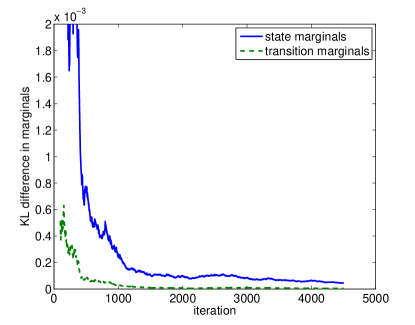
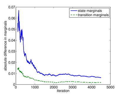
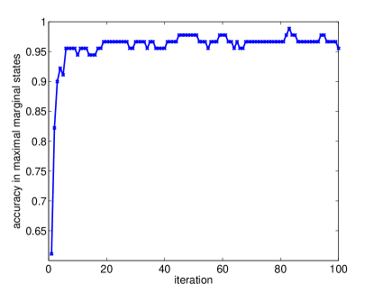
We want to examine the accuracy of the proposed approximation against the exact methods, along the three dimensions: (i) the state marginals at time and depth level , (ii) the probability that a transition occurs at time , and (iii) the decoding accuracy using . For the first two estimations, two accuracy measures are used: a) the average Kullback-Leibler divergence between state marginals and b) the average absolute difference in state marginals. For decoding evaluation, we use the percentage of matching between the maximal states.
Convergence behaviours for a fixed sequence length: Figures 3 and 4 show the three measures using the one-long-run strategy (up to iterations). It appears that both the KL-divergence and absolute difference continue to decrease, although it occurs at an extremely slow rate after iterations. The maximal state measure is interesting: it quickly reaches the high accuracy after just iterations. In other words, the mode of the state marginal is quickly located although the marginal has yet to converge.
 |
 |
| (a) | (b) |
 |
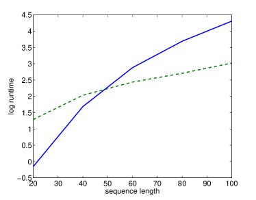
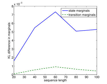
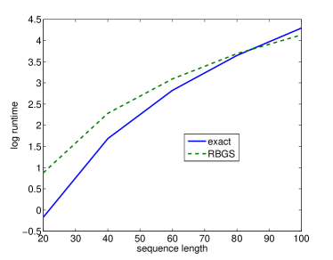
Convergence as a function of sequence length: To test how the RBGS scales, three experiments with different run times are performed:
-
•
The number of iterations is fixed at for all sequence lengths. This gives us a linear run time in term of .
-
•
The number of iterations scales linearly with , and thus the total cost is .
-
•
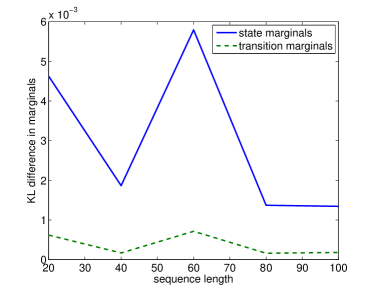
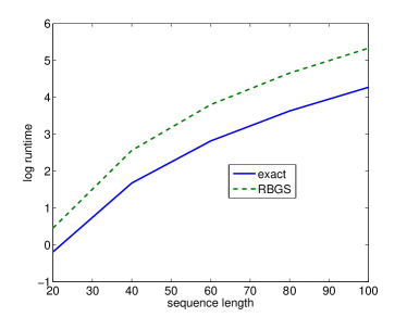
The number of iterations scales quadratically with . This costs , which means no saving compared to the exact inference.
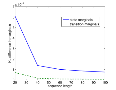
The long data is obtained by simply concatenating the original sequences many times. The sequence lengths are . Figure 5(a,b) show the performance of the RBGS in linear run-time with respect to sequence length. Figure 5a depicts the actual run-time for the exact and RBGS inference. Figure 5b plots the KL-divergences between marginals obtained by the exact method and by the RBGS. Performance of the RBGS for quadratic and cubic run-times is shown in Figure 6(a,b) and Figure 7(a,b), respectively.
 |
 |
| (a) log-run time | (b) KL divergence |
 |
 |
| (a) log-run time | (b) KL divergence |
 |
 |
| (a) log-run time | (b) KL divergence |
5 Relations with Other Deep Architectures
Deep neural architectures (DNA) such as Deep Belief Networks [9] and Deep Boltzmann Machines [13] have recently re-emerged as a powerful modelling framework which can potentially discover high-level semantics of the data. The HSCRF shares some similarity with the DNA in the way that they both use stacking of simpler building blocks. The purpose is to capture long-range dependencies or higher-order correlations which are not directly evident in the raw data. The building blocks in the HSCRF are the chain-like Conditional Random Fields, while they are the Restricted Boltzmann Machines in the DNA. These building blocks are different, and as a result, the HSCRF is inherently sequential and localised in state representation, while the DNA was initially defined for non-sequential data and distributed representation. In general, the distributed representation is richer as it carries more bits of information given a number of hidden units. The drawback is that probabilistic inference of RBM and its stacking is intractable, and thus approximation techniques such as MCMC and mean-field are often used. Inference in the HSCRF, on the other hand, is polynomial. For approximation, the MCMC technique proposed for the HSCRF in this paper exploits the efficiency in localised state representation so that the Rao-Blackwellisation can be used.
Perhaps the biggest difference between the HSCRF and DNA is the modelling purpose. More specifically, the HSCRF is mainly designed for discriminative mapping between the sequential input and the nested states, usually in a fully supervised fashion. The states often have specific meaning (e.g. noun-phrase, verb-phrase in sentence modelling). On the other hand, DNA is for discovering hidden features, whose meanings are often unknown in advance. Thus, it is generative and unsupervised in nature. Finally, despite this initial difference, the HSCRF can be readily modified to become a generative and unsupervised version, such as the one described in [16, Ch. 9].
Training in HSCRFs can be done simultaneously across all levels, while for the DNA it is usually carried out in a layer-wise fashion. The drawback of the layer-wise training is that errors made by the lower layers often propagate to the higher. Consequently, an extra global fine tuning step is often employed to correct them.
There have been extensions of the Deep Networks to sequential patterns such as Temporal Restricted Boltzmann Machines (TRBM) [15] and some other variants. The TRBM is built by stacking RBMs both in depth and time. Another way to build deep sequential model is to feed the top layer of the Deep Networks into the chain-like CRF, as in [4].
6 Conclusion
We have introduced a novel technique known as Rao-Blackwellised Gibbs Sampling (RBGS) for approximate inference in the Hierarchical Semi-Markov Conditional Random Fields. The goal is to avoid both the cubic-time complexity in the standard Inside-Outside algorithms and the exponential states in the DBN representation of the HSCRFs. We provide some simulation-based evaluation of the quality of the RGBS with respect to run time and sequence length.
This work, however, is still at an early stage and there are promising directions to follow. First, there are techniques to speed up the mixing rate of the MCMC sampler. Second, the RBGS can be equipped with the Contrastive Divergence [8] for stochastic gradient learning. And finally, the ideas need to be tested on real, large-scale applications with arbitrary length and depth.
References
- [1] H. H. Bui, D. Q. Phung, and S. Venkatesh. Hierarchical hidden Markov models with general state hierarchy. In D. L. McGuinness and G. Ferguson, editors, Proceedings of the 19th National Conference on Artificial Intelligence (AAAI), pages 324–329, San Jose, CA, Jul 2004.
- [2] H. H. Bui, S. Venkatesh, and G. West. Policy recognition in the abstract hidden Markov model. Journal of Artificial Intelligence Research, 17:451–499, 2002.
- [3] G. Casella and C.P. Robert. Rao-Blackwellisation of sampling schemes. Biometrika, 83(1):81, 1996.
- [4] Trinh-Minh-Tri Do and Thierry Artieres. Neural conditional random fields. In NIPS Workshop on Deep Learning for Speech Recognition and Related Applications, 2009.
- [5] A. Doucet, N. de Freitas, K. Murphy, and S. Russell. Rao-Blackwellised particle filtering for dynamic Bayesian networks. In Proceedings of the Sixteenth Conference on Uncertainty in Artificial Intelligence, pages 176–183. Citeseer, 2000.
- [6] Shai Fine, Yoram Singer, and Naftali Tishby. The hierarchical hidden Markov model: Analysis and applications. Machine Learning, 32(1):41–62, 1998.
- [7] S. Geman and D. Geman. Stochastic relaxation, Gibbs distributions, and the Bayesian restoration of images. IEEE Transactions on Pattern Analysis and Machine Intelligence (PAMI), 6(6):721–742, 1984.
- [8] G.E. Hinton. Training products of experts by minimizing contrastive divergence. Neural Computation, 14:1771–1800, 2002.
- [9] G.E. Hinton and R.R. Salakhutdinov. Reducing the dimensionality of data with neural networks. Science, 313(5786):504–507, 2006.
- [10] J. Lafferty, A. McCallum, and F. Pereira. Conditional random fields: Probabilistic models for segmenting and labeling sequence data. In Proceedings of the International Conference on Machine learning (ICML), pages 282–289, 2001.
- [11] K. Murphy and M. Paskin. Linear time inference in hierarchical HMMs. In Advances in Neural Information Processing Systems (NIPS), volume 2, pages 833–840. MIT Press, 2002.
- [12] Lawrence R. Rabiner. A tutorial on hidden Markov models and selected applications in speech recognition. Proceedings of the IEEE, 77(2):257–286, 1989.
- [13] R. Salakhutdinov and G. Hinton. Deep Boltzmann Machines. In Proceedings of 20th AISTATS, volume 5, pages 448–455, 2009.
- [14] Sunita Sarawagi and William W. Cohen. Semi-Markov conditional random fields for information extraction. In Bottou L Saul LK, Weiss Y, editor, Advances in Neural Information Processing Systems 17, pages 1185–1192. MIT Press, Cambridge, Massachusetts, 2004.
- [15] I. Sutskever and G.E. Hinton. Learning multilevel distributed representations for high-dimensional sequences. In Proceeding of the Eleventh International Conference on Artificial Intelligence and Statistics, pages 544–551, 2007.
- [16] Tran The Truyen. On Conditional Random Fields: Applications, Feature Selection, Parameter Estimation and Hierarchical Modelling. PhD thesis, Curtin University of Technology, 2008.
- [17] T.T. Truyen, D.Q. Phung, H.H. Bui, and S. Venkatesh. Hierarchical Semi-Markov Conditional Random Fields for recursive sequential data. In Twenty-Second Annual Conference on Neural Information Processing Systems (NIPS), Vancouver, Canada, Dec 2008.