Resonant Chains and Three-body Resonances in the Closely-Packed Inner Uranian Satellite System

Abstract

Numerical integrations of the closely-packed inner Uranian satellite system show that variations in semi-major axes can take place simultaneously between three or four consecutive satellites. We find that the three-body Laplace angle values are distributed unevenly and have histograms showing structure, if the angle is associated with a resonant chain, with both pairs of bodies near first-order two-body resonances. Estimated three-body resonance libration frequencies can be only an order of magnitude lower than those of first-order resonances. Their strength arises from a small divisor from the distance to the first-order resonances and insensitivity to eccentricity, which make up for their dependence on moon mass. Three-body resonances associated with low-integer Laplace angles can also be comparatively strong due to the many multiples of the angle contributed from Fourier components of the interaction terms. We attribute small coupled variations in semi-major axis, seen throughout the simulation, to ubiquitous and weak three-body resonant couplings. We show that a system with two pairs of bodies in first-order mean-motion resonance can be transformed to resemble the well-studied periodically-forced pendulum with the frequency of a Laplace angle serving as a perturbation frequency. We identify trios of bodies and overlapping pairs of two-body resonances in each trio that have particularly short estimated Lyapunov timescales.

1 Introduction

Uranus has the most densely-packed system of low-mass satellites in the solar system, having 13 low-mass inner moons with semi-major axes between $a=49,752-97,736$ km or 1.9– 3.8 Uranian radii (Smith et al., 1986; Karkoschka, 2001; Showalter & Lissauer, 2006). The satellites are named after characters from Shakespeare’s plays and in order of increasing semi-major axis are Cordelia, Ophelia, Bianca, Cressida, Desdemona, Juliet, Portia, Rosalind, Cupid, Belinda, Perdita, Puck and Mab. External to these moons, Uranus has five larger classical moons (Miranda, Ariel, Umbriel, Titania and Oberon) and a number of more distant irregular satellites.

Signatures of gravitational instability were first revealed in long-term numerical N-body integrations by Duncan & Lissauer (1997), who predicted collisions between Uranian satellites in only 4–100 million years. Observations by Voyager 2 and the Hubble Space Telescope have shown that the orbits of the inner satellites are variable on timescales as short as two decades (Showalter & Lissauer, 2006; Showalter et al., 2008, 2010). Recent numerical studies (Dawson et al., 2010; French & Showalter, 2012) suggest that the instability is due to multiple mean-motion resonances between pairs of satellites. French & Showalter (2012) predict that the pairs Cupid/Belinda or Cressida/Desdemona have orbits that will cross within $10^{3}-10^{7}$ years, an astronomically short timescale.

Numerical studies of two orbiting bodies find that stable and unstable regimes are separated by sharp boundaries (e.g., Gladman 1993; Mudryk & Wu 2006; Mardling 2008; Mustill & Wyatt 2012; Deck et al. 2013). In contrast, numerical studies of closely-packed planar orbiting systems describe stability with power-law relations (Duncan & Lissauer, 1997; Chambers et al., 1996; Smith & Lissauer, 2009). Systems are integrated until the orbit of one body crosses the orbit of another body and this time, the crossing timescale, depends on powers of the mass and the initial separation of the orbits (Duncan & Lissauer, 1997; Chambers et al., 1996; Smith & Lissauer, 2009). The stability boundary in three-body systems is attributed to overlap of resonances involving two bodies (Wisdom, 1980; Culter, 2005; Mudryk & Wu, 2006; Quillen & Faber, 2006; Mardling, 2008; Mustill & Wyatt, 2012; Deck et al., 2013). In contrast, Quillen (2011) proposed that the power law relations in multiple-body systems were due to resonance overlap of multiple weak three-body resonances and the strong sensitivity of these three-body resonance strengths to masses and inter-body separations.

In this study we probe in detail one of the numerical integrations of the Uranian satellite system presented by French & Showalter (2012), focusing on resonant processes responsible for instability in multiple-body systems. In section 2 we describe the numerical integration and we compute estimates for boundaries of stability. In section 4 we construct a Hamiltonian model for the dynamics of a coplanar, low-mass multiple-satellite or -planet system using a low-eccentricity expansion. In section 5 we estimate the libration frequencies of the strong two-body first-order resonances in the Uranian satellite system. In section 6 we search for three-body resonances between bodies. The strengths of three-body resonances that are near two-body first-order resonances are computed in section 7.1 and a timescale for chaotic evolution estimated for a resonant chain consisting of pairs of bodies in mean-motion resonance in section 7.3. In section 7.4 we estimate the strength of three-body resonances that have Laplace angles with low indices. A summary and discussion follows in section 8.

2 The Numerical Integration and Observed Resonances

The numerical integration we use in this study is one of those presented and described in detail by French & Showalter (2012). This simulation integrates the 13 inner moons (from Cordelia through Mab) in the Uranian satellite system using the SWIFT software package. The adopted planet radius is $R_{U}=26,200$ km (as by Duncan & Lissauer 1997), the quadrupole and octupole gravitational moments for Uranus are $J_{2}=3.34343\times 10^{-3}$ and $J_{4}=-2.885\times 10^{-5}$ (as by French et al. 1991), and the mass for Uranus is $GM_{U}=5793965.663939$ km³s^-2 (following French & Showalter 2012). The integrations do not include the five classical moons (Miranda, Ariel, Umbria, Titania and Oberon) as they do not influence the stability of the inner moons (Duncan & Lissauer, 1997; French & Showalter, 2012).

The masses of the inner moons that we adopt, and specifying the integration amongst those presented by French and Showalter, are those given in the middle column of Table 1 of French & Showalter (2012). They are estimated from the observed moon radii assuming a density of 1.0 g cm^-3. Initial conditions for the numerical integration in the form of a state vector (position and velocity) for each moon and dependent on the assumed moon masses, were determined through integration and iterative orbital fitting and are consistent with observations for the first 24 years over which astrometry was available (French & Showalter, 2012).

Table 1: Initial integration parameters

Satellite	$a$(km)	$e$	$m$	$n$(Hz)	$\omega/n$
Cordelia	49751.8	0.00024	4.47e-10	2.1706e-04	1.40e-03
Ophelia	53763.7	0.01002	5.87e-10	1.9320e-04	1.20e-03
Bianca	59165.7	0.00096	9.50e-10	1.6734e-04	9.87e-04
Cressida	61766.8	0.00035	3.33e-09	1.5687e-04	9.05e-04
Desdemona	62658.3	0.00023	2.07e-09	1.5354e-04	8.80e-04
Juliet	64358.3	0.00074	7.18e-09	1.4749e-04	8.34e-04
Portia	66097.4	0.00017	1.66e-08	1.4170e-04	7.90e-04
Rosalind	69927.0	0.00033	2.25e-09	1.3022e-04	7.06e-04
Cupid	74393.1	0.00170	3.52e-11	1.1867e-04	6.23e-04
Belinda	75255.8	0.00027	4.40e-09	1.1663e-04	6.09e-04
Perdita	76417.1	0.00351	1.06e-10	1.1398e-04	5.91e-04
Puck	86004.7	0.00009	2.56e-08	9.5457e-05	4.66e-04
Mab	97736.3	0.00246	8.34e-11	7.8792e-05	3.61e-04

The semi-major axis, $a$ (in km), and eccentricity, $e$, are initial geometrical orbital elements for the numerical integration studied here, and presented and described by French & Showalter (2012). The ratio of the mass of the moon to the planet is given as $m$. Masses are based on the observed radii assuming a density of 1 g cm^-3, and are consistent with those listed in the middle column of Table 1 of French & Showalter (2012). Mean motions, $n$, are in units of Hz. The unitless $\omega/n$ is the ratio of precession rate to mean motion.

Using the state vectors output by the integrations, we compute the geometric orbital elements of Borderies-Rappaport & Longaretti (1994), as implemented in closed-form solution by Renner & Sicardy (2006), because they are not subject to the short-term oscillations present in the osculating elements caused by Uranus’s oblateness. For each moon, initial semi-major axis, $a$, and eccentricity, $e$, are listed in Table 1, along with mean motion, $n$, secular precession frequency, $\omega$, and the ratio of the moon to planet mass, $m$.

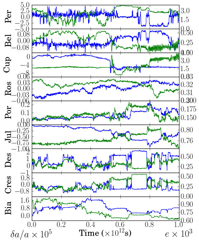
Figure 1: Semi-major axes and eccentricities of the inner Uranian moons during the first part of the numerical integration. Not all moons are plotted; see 2. Plotted as blue lines and with the $y$-axis on the left are deviations $(a-a_{0})/a_{0}\times 10^{5}$ where $a$ is the semi-major axis and $a_{0}$ is its initial value for each moon. The green lines show the eccentricities $\times 10^{3}$ with the $y$-axis on the right. Scaling factors are written on the lower left and right. This figure illustrates coupled variations in semi-major axis between two, three or four bodies. Anti-correlated variations in eccentricity and semi-major axis are evident for the lower-mass body when two bodies are in a first- or second-order mean-motion resonance.

The integration output contains state vectors for the 13 inner satellites at times separated by $10^{7}$ s and the integration is $t=3.6\times 10^{12}$s long ($1.2\times 10^{5}$ yr). We focus on the first part of the integration ($t<10^{12}$s), when the variations in the bodies have not deviated significantly from their initial semi-major axes and eccentricities, and before Cupid and Belinda enter a regime of first-order resonance overlap, jumping from resonance to resonance (as illustrated by French & Showalter 2012, see their Figures 2 and 3). To average over short timescale variations in the orbital elements, we computed median values of the semi-major axes and eccentricities in time intervals $10^{9}$s long (and consisting of 100 recorded states for this integration). These are shown to $t=10^{12}$s in Figure 1. The semi-major axes as a function of time are plotted as a unitless ratio $(a-a_{0})/a_{0}\times 10^{5}$ where $a_{0}$ is the initial semi-major axis and the eccentricities are shown multiplied by $10^{3}$.

Figure 1 shows that variations in semi-major axes between bodies are correlated. As pointed out by French & Showalter (2012), there are a number of strong first-order mean-motion resonances. Cressida and Desdemona are near the 43:44 mean-motion resonance, Bianca and Cressida are near the 15:16 resonance, and Belinda and Perdita are near the 43:44 resonance. Juliet and Portia are near the 49:51 second-order mean-motion resonance.

A $p-1:p$ first-order resonance between body $i$ and body $j$ is described with one of the following resonant angles:

$$\phi_{pi} = p\lambda_{j}+(1-p)\lambda_{i}-\varpi_{i}$$

$$\phi_{pj} = p\lambda_{j}+(1-p)\lambda_{i}-\varpi_{j}$$ (1)

where $p$ is an integer, $\lambda_{i},\lambda_{j}$ are the mean longitudes of bodies $i$ and $j$. The angles $\varpi_{i},\varpi_{j}$ are the longitudes of pericenter. These angles move slowly when there is a commensurability between the mean motions $n_{i},n_{j}$,

$$pn_{j}\approx(p-1)n_{i}.$$ (2)

The resonant argument $\phi_{pi}$ tends to be more important when the $i$-th body is the lighter body and $\phi_{pj}$ is more important if the $j$-th body is lighter.

In comparing semi-major axis variations with eccentricity variations, we see that semi-major axis variations in two nearby bodies can be inversely correlated and the eccentricity variations of the lower-mass body tend to be anti-correlated with its semi-major axis variations. As we will review in section 5, within the context of a Hamiltonian model, when a single resonant argument is important (that associated with $\phi_{pi}$ or $\phi_{pj}$), conserved quantities relate variations in the semi-major axes to the eccentricity of one of the bodies.

Figure 1 shows that at times there are simultaneous variations between three or four bodies. The semi-major axes of Cressida, Desdemona, Juliet and Portia often exhibit simultaneous variations with Cressida and Desdemona moving in opposite directions, Juliet and Portia moving in opposite directions and Desdemona and Juliet moving in the same direction. The correlated variations in semi-major axes seen in Figure 1 between more than one body are similar to the variations exhibited by integrated closely-spaced planetary systems (e.g., see Figure 3 of Quillen 2011) that were interpreted in terms of coupling between consecutive bodies from three-body resonances. We will investigate this possibility below.

Eccentricities, however, are less well correlated. Often two bodies experience opposite or anti-correlated eccentricity variations. For two bodies with similar masses, the two resonant arguments, $\phi_{pi},\phi_{pj}$, are of equal importance or strength. Cressida and Desdemona have similar masses and so the 46:47 resonance causes anti-correlated eccentricity variations in the two moons. But rarely are eccentricity variations simultaneous among three or more bodies. This might be expected as the eccentricities of these satellites are low (see Table 1), and so high-order (in eccentricity) terms and secular terms in the expansion of the two-body interactions in the Hamiltonian or the disturbing function are weak.

3 Stability boundary estimates

Here we expand on the predictions of stability estimated by French & Showalter (2012) in their section 3.1. A seminal stability measurement for a two-planet system is that by Gladman (1993). We define a normalized distance between the semi-major axes of two bodies with semi-major axes $a_{i},a_{j}$ as

$$\Delta\equiv(a_{j}-a_{i})/a_{i},$$ (3)

and we assume $a_{i}<a_{j}$. Gladman’s numerical study showed that a coplanar system with a central body and two close planets on circular orbits is Hill stable (does not ever undergo close encounters) as long as the initial separation $\Delta\la\Delta_{G}$ with

$$\Delta_{G}\equiv 2.4(m_{i}+m_{j})^{1/3}.$$ (4)

Here $m_{i}$ and $m_{j}$ are the planet masses divided by that of the central star.

Chambers et al. (1996) explored equal-mass and equally-spaced but multiple-planet planar systems finding that $\Delta\la\Delta_{C}$ is required for Hill stability with

$$\Delta_{C}\equiv 10R_{mH}/a_{i}$$ (5)

and $\Delta$ computed between a consecutive pair of planets. Here the mutual Hill radius

$$R_{mH}\equiv\left({m_{i}+m_{j}\over 3}\right)^{1/3}\left({a_{i}+a_{j}\over 2}\right).$$ (6)

In the planar restricted three-body system, a low-mass object in a nearly-circular orbit near a planet in a circular orbit is likely to experience close approaches with a planet when $\Delta\la\Delta_{W}$ with

$$\Delta_{W}\equiv 1.5m^{2/7},$$ (7)

where $m$ is the mass ratio of the planet to the star. This relation is known as the 2/7-th law and the exponent is predicted by a first-order mean-motion resonance overlap criterion (Wisdom, 1980). The coefficient predicted by Wisdom (1980) is 1.3, but numerical studies suggest it could be as large as 2 (Chiang et al., 2009); here we have adopted an intermediate value of 1.5. For a low-mass body apsidally aligned with a low but non-zero eccentricity planet, the 2/7-th law is unchanged for bodies with low initial free-eccentricity (Quillen & Faber, 2006); otherwise the chaotic zone boundary is near

$$\Delta_{e}\equiv 1.8(me)^{1/5},$$ (8)

where $e$ is the low-mass body’s eccentricity (Culter, 2005; Mustill & Wyatt, 2012). This relation is known as the 1/5-th law.

For consecutive pairs of Uranian satellites we compute these four measures of Hill stability using initial state vectors for each body as described in section 2 and listed in Table 1. The 2/7-th and 1/5-th laws are derived for a massless body near a planet but here all the bodies have mass. For each consecutive pair we use the maximum masses and eccentricities, computing the boundaries (in normalized semi-major axis) as

$$\Delta_{W} = 1.5\left[\max(m_{i},m_{j})\right]^{2\over 7}$$

$$\Delta_{e} = 1.8\left[\max(m_{i},m_{j})\max(e_{i},e_{j})\right]^{1\over 5}.$$ (9)

In section 5 below, we estimate the first-order resonance width for two massive bodies and explain why we use the maximum mass in these distances.

The four measures of stability, $\Delta_{G},\Delta_{C},\Delta_{W},$ and $\Delta_{e}$ are listed in Table 2. We expect instability if $\Delta$ divided by any of these measures is less than 1. All measures of stability suggest that the inner Uranian satellite system could be stable. However, four pairs of consecutive satellites are near estimated boundaries of instability. These pairs are Cressida/Desdemona, Juliet/Portia, Cupid/Belinda and Belinda/Perdita. The stability boundaries suggest that Cordelia and Ophelia are dynamically distant from the remaining bodies as are Puck and Mab. Bianca through Rosalind are close together as are Cupid through Perdita. Cordelia, Ophelia, Puck and Mab are not plotted in Figure 1 because they exhibited minimal variations in orbital elements and lacked variations that coincided with variations in the elements of the other moons.

An evenly spaced equal mass multiple body system with $\Delta=1.2\Delta_{C}$ and a mass ratio of $10^{-9}$ has a crossing timescale $\sim 10^{10}$ orbital periods. (from Figure 3 by Chambers et al. 1996). Using an orbital period for Cressida of about 11 hours this corresponds to $10^{7}$ years, exceeding the crossing timescales measured by French & Showalter (2012) by an order of magnitude (see their Table 3). The measured crossing timescale is shorter than that of the equally spaced system because pairs of bodies (like Cressida and Desdemona or Cupid and Belinda) are in or near first order mean motion resonances. They are near first order resonances possibly because these resonances fill a larger fraction of phase space volume when two bodies have nearby orbits. (The measure $\Delta_{W}$ is related to a first order resonance overlap condition). The closest two bodies are usually the first to cross orbits and so can set the numerically measured crossing timescale in a multiple body system.

Table 2: Stability estimates from pairs of moons

Pair of Moons		$\Delta$	${\Delta\over\Delta_{G}}$	${\Delta\over\Delta_{C}}$	${\Delta\over\Delta_{W}}$	${\Delta\over\Delta_{e}}$
Cordelia	Ophelia	0.081	33.2	11.1	23.3	7.9
Ophelia	Bianca	0.100	36.3	12.0	25.3	8.9
Bianca	Cressida	0.044	11.3	3.8	7.8	4.9
Cressida	Desdemona	0.014	3.4	1.2	2.5	2.0
Desdemona	Juliet	0.027	5.4	1.8	3.8	2.7
Juliet	Portia	0.027	3.9	1.3	3.0	2.3
Portia	Rosalind	0.058	9.1	3.1	6.5	5.8
Rosalind	Cupid	0.064	20.2	6.8	12.6	6.8
Cupid	Belinda	0.012	2.9	1.0	1.9	1.1
Belinda	Perdita	0.015	3.9	1.3	2.5	1.2
Perdita	Puck	0.125	17.7	5.8	12.3	7.1
Puck	Mab	0.136	19.3	6.2	13.4	8.3

Here $\Delta\equiv(a_{i+1}-a_{i})/a_{i}$ gives the separation between consecutive bodies $i$ and $i+1$. The fourth through seventh columns list $\Delta$ divided by $\Delta_{G},\Delta_{C},\Delta_{W}$ and $\Delta_{e}$, delimiting different stability estimates. None of the values listed here imply that the system will experience close encounters, though the Cressida/Desdemona, Juliet/Portia, Cupid/Belinda, and Belinda/Perdita pairs have lowest ratios and so are pairs of moons nearest to regions of instability.

While there might be a sharp boundary between stable and unstable systems when there are only two planets, in a multiple-body system the body masses and separations instead define an evolutionary timescale. With initial conditions consisting of orbits that do not intersect (when projected onto the mid-plane), a proxy for a stability timescale is the time for one body to have an orbit that crosses the orbit of another body. This crossing timescale, measured numerically, has been fit by a function that is proportional to a power of the masses and a power of the interplanetary separations (Chambers et al., 1996; Duncan & Lissauer, 1997; Smith & Lissauer, 2009; French & Showalter, 2012). The numerically measured exponents in these studies are not identical and may depend on the number of bodies in the system, initial eccentricities (e.g. Zhou et al. 2007), the masses of the individual bodies when not all masses are equal, and their initial spacings if they are not equidistant.

Chaotic diffusion occurs in regions where resonances overlap (e.g. Chirikov 1979; Wisdom 1980; Holman & Murray 1996; Murray & Holman 1997; Nesvorný & Morbidelli 1998a; Murray et al. 1998; Quillen 2011; Giuppone et al. 2013). The 2/7-th law is derived by computing the location where first-order mean-motion resonances between two bodies in nearly circular orbits are sufficiently wide and close together that they overlap (Wisdom, 1980; Deck et al., 2013). In contrast, Gladman (1993) accounted for the Hill stability boundary of two-planet systems with an estimate for a critical value for Hill stability, derived by Marchal & Bozis (1982), at which bifurcation in phase space topology occurs.

The average mass ratio of the moons from Bianca to Perdita is $\mu\approx 4\times 10^{-9}$ so the inner Uranian satellites are at the low mass end of the evenly spaced equal mass compact systems numerically studied by Chambers et al. (1996). Using the fitted relation by Faber & Quillen (2007) and mass ratio $\mu=4\times 10^{-9}$ we estimate the crossing time for equally spaced, equal mass multiple body systems, finding $\sim 10^{7}$ orbital periods for a spacing of $\Delta=0.014$ (similar to the closest pairs in the inner Uranian satellite system) and $\sim 10^{13}$ periods for $\Delta=0.03$ (approximately the mean spacing for moons from Bianca to Perdita). In comparison, the crossing timescale numerically estimated by French & Showalter (2012) is $\sim 10^{6}$ years or $\sim 10^{9}$ orbital periods (using an orbital period for Cressida of about 11 hours). The closest pairs of bodies drastically lower the crossing timescale of the whole system with the closest two bodies usually the first to cross orbits. But integration of a close pair of bodies in isolation does not give a good estimate for the crossing timescale in the full multiple body system.

Three-body mean motion resonances among the mean motions of an asteroid, Jupiter and Saturn are denser than ordinary mean motion resonances (Nesvorný & Morbidelli, 1998a; Smirnov & Shevchenko, 2013). Overlap of three-body resonance multiplets is an important source of chaos in the asteroid belt (Nesvorný & Morbidelli, 1998a; Murray et al., 1998). Recently, Quillen (2011) proposed that chaotic evolution of planar, equal mass, closely-spaced, planetary systems is due to three-body resonances and estimated their strengths using zeroth-order (in eccentricity) two-body interaction terms. Crossing timescales were estimated from the time for a system to cross into a first-order mean-motion resonance between two bodies. The sensitivity of the three-body resonances to interplanetary spacing and planet mass, and the associated diffusion caused by them, could account for the range of crossing timescales measured numerically in compact multiple-planet systems. Laplace coefficients are exponentially sensitive to the Fourier integer coefficients and this limits the maximum resonance index and so the number of three-body resonances that can be important in any particular system. Equivalently, the index is truncated at smaller integers for more widely-separated bodies, limiting the interactions between non-consecutive bodies and accounting for the insensitivity of the crossing time scales to the number of bodies integrated (Quillen, 2011).

Three-body resonance strengths were previously estimated by Quillen (2011) assuming that pairs of bodies were distant from two-body resonances. However, the Uranian system contains pairs of moons in two-body resonance and intermittent resonant behavior is clearly seen in the numerical integrations by French & Showalter (2012); by intermittent behavior we mean that there are intervals of time with slow smooth evolution separated by intervals with rapid chaotic transitions. The proximity of pairs of bodies to the 2/7th and 1/5th law boundaries implies that even if the first order resonances are not overlapping, the system is strongly affected by them.

Dawson et al. (2010) previously suggested that the chaotic behavior in the Uranian satellite system is due to this web of two-body resonances. To improve upon the estimate of Quillen (2011), we take into account the uneven spacing and different satellite masses when estimating three-body resonance strengths, and we also take into account the two-body mean-motion resonances.

4 A nearly-Keplerian Hamiltonian Model for coplanar Multiple-Body dynamics

The inner moons of Uranus have low masses and eccentricities (see Table 1), so a lower-order expansion in satellite mass and eccentricity should be sufficient to capture the complexity of the dynamics. In this section we use a Hamiltonian to describe multiple-body interactions in such a nearly-Keplerian setting. This approach is similar to that previously done by Quillen (2011) (but also see Holman & Murray 1996; Deck et al. 2013). For simplicity we describe our formulation in terms of moons orbiting a central planet, but without loss of generality the same formulation could be applied to planets orbiting a central star.

The Hamiltonian for $N$ non-interacting massive bodies orbiting a planet (and so feeling gravity only from the central planet) can be written as a sum of Keplerian terms

$$H_{Kep}=\sum_{j=1}^{N}-{m_{j}^{3}\over 2\Lambda_{j}^{2}}$$ (10)

where $m_{j}$ is the mass of the $j$-th body divided by the mass of planet, $M_{p}$. We have ignored the motion of the planet and have put the above Hamiltonian in units such that $GM_{p}=1$, where $G$ is the gravitational constant. Here the Poincaré momentum

$$\Lambda_{j}=m_{j}\sqrt{a_{j}},$$ (11)

where the semi-major axis of the $j$-th body is $a_{j}$ and the associated mean motion is $n_{j}$. This Poincaré coordinate is conjugate to the mean longitude, $\lambda_{j}$, of the $j$-th body. The mean longitude, $\lambda_{j}=M_{j}+\varpi_{j}$, where $M_{j}$ is the mean anomaly and $\varpi_{j}$ is the longitude of pericenter of the $j$-th body and we have assumed a planar system and so neglected the longitude of the ascending node. We also use the Poincaré coordinate

$$\Gamma_{j}=m_{j}\sqrt{a_{j}}(1-\sqrt{1-e_{j}^{2}})\approx m_{j}\sqrt{a_{j}}\frac{e_{j}^{2}}{2},$$ (12)

where $e_{j}$ is the $j$-th body’s eccentricity. This coordinate is conjugate to the angle $\gamma_{j}=-\varpi_{j}$. We note that the Poincaré momenta retain a factor of satellite’s mass. We ignore the vertical degree of freedom.

Interactions between pairs of bodies contribute to the Hamiltonian with a term

$$H_{Int}=\sum_{j>i}W_{ij}$$ (13)

with

$$W_{ij}=-{m_{i}m_{j}\over|{\bf r}_{i}-{\bf r}_{j}|}.$$ (14)

Here ${\bf r}_{i}$ are the coordinates with respect to the central mass of the $i$-th body.

We choose to work in planet-centric coordinates. The momenta conjugate to planet-centric coordinates are barycentric momenta (see for example section 4 of Duncan et al. 1998 and Wisdom, Holman & Touma 1996 for heliocentric coordinates). The N-body Hamiltonian gains an additional term $H_{drift}$, arising from the use of the planet-centric coordinate system;

$$H_{drift}={1\over 2M_{p}}\left|\sum_{i=1}^{N}{\bf P}_{i}\right|^{2}$$ (15)

(following equation 3b of Duncan et al. 1998). Here ${\bf P}_{i}$ is the barycentric momentum of the $i$-th body and the sum is over all bodies except the central body. Some attention must be taken to ensure that the above expression has units consistent with $GM_{p}=1$. Expansion of $H_{drift}$ gives the indirect terms in the expansion of the disturbing function in the Lagrangian rather than Hamiltonian setting.

The central body could be an oblate planet. The difference between a point mass and an oblate mass can be described with a perturbation term, $H_{ob}$, that is the sum of the quadrupolar and higher moments of the planet’s gravitational potential. Altogether the Hamiltonian is

$$H=H_{Kep}+H_{Int}+H_{Drift}+H_{ob}.$$ (16)

An additional term could also be added to take into account post-Newtonian corrections.

4.1 Some notation

We focus here on the regime of closely-spaced, low-mass, planar systems. We define the difference of mean motions

$$n_{ij}\equiv n_{i}-n_{j}\sim\frac{3}{2}\delta_{ij}$$ (17)

when $\delta_{ij}$ is small. Here $\delta_{ij}$ is an inter-body separation with

$$\delta_{ij}\equiv\alpha_{ij}^{-1}-1\approx 1-\alpha_{ij}$$ (18)

and the ratio of semi-major axes

$$\alpha_{ij}\equiv a_{i}/a_{j}.$$ (19)

We use a convention $a_{i}<a_{j}<a_{k}$ when three bodies are discussed so that $\alpha_{ij},\alpha_{jk}<1$. It is convenient to define differences of longitudes of pericenter and mean longitudes

$$\lambda_{ij} \equiv \lambda_{i}-\lambda_{j}$$

$$\varpi_{ij} \equiv \varpi_{i}-\varpi_{j}$$ (20)

for bodies $i,j$.

Interaction strengths depend on Laplace coefficients,

$$b_{s}^{(q)}(\alpha)\equiv{1\over\pi}\int_{0}^{2\pi}{\cos(q\phi)d\phi\over(1+\alpha^{2}-2\alpha\cos\phi)^{s}},$$ (21)

where $q$ is an integer and $s$ a positive half integer. Laplace coefficients are the Fourier coefficients of twice the function $f(\phi)=(1+\alpha^{2}-2\alpha\cos\phi)^{-s}$. As this function is locally analytic, the Fourier coefficients decay rapidly at large $q$ and the rate of decay is related to the width of analytical continuation in the complex plane (Quillen, 2011). When the two objects are closely-spaced ($\alpha_{ij}\sim 1$), the Laplace coefficient can be approximated

$$b^{(p)}_{1/2}(\alpha_{ij})\sim 0.5|\log\delta_{ij}|\exp(-p\delta_{ij})$$ (22)

(see equation 10 and Figure 1 of Quillen 2011).

As long as the central body is much more massive than the other bodies and the bodies are not undergoing close encounters, the terms $H_{Int},H_{Drift},H_{ob}$ in the above Hamiltonian can be considered perturbations to the Keplerian Hamiltonian, $H_{Kep}$. Each of these terms can be expanded in orders of eccentricity and in a Fourier series so that each term contains a cosine of an angle or argument, $\phi_{\bf k}$, that depends on a sum of the Poincaré angles, $\phi_{\bf k}={\bf k}\cdot(\vec{\lambda},\vec{\gamma})$ where ${\bf k}$ is a vector of integers and $\vec{\lambda},\vec{\gamma}$ are vectors of mean longitudes and negative longitudes of pericenter for all bodies. The coefficients for each argument are functions of the Poincaré momenta. Expansion of the pair interaction terms is referred to as expansion of the disturbing function and is outlined in Chapter 6 of Murray & Dermott (1999) and other texts. The expansion is also done in their chapter 8 using a Hamiltonian approach and in terms of Poincaré coordinates for each body. A low-eccentricity expansion for $W_{ij}$ can be put in Poincaré coordinates using the relations between semi-major axis and eccentricity and Poincaré momenta $\vec{\Gamma},\vec{\Lambda}$. We focus here on low-eccentricity terms in the Hamiltonian or those that depend on the momenta $\Gamma_{j}$ to half powers less than or equal to 2 (or eccentricity to a power less than or equal to 4). Terms in the expansion that do not depend on mean longitudes are called secular terms. Secular terms are divided into two classes, those that depend on longitudes of pericenter ($\vec{\varpi}$) and those that are independent of all Poincaré angles. Interactions between bodies give both types of secular perturbation terms, whereas the oblateness of the planet only affects the precession rates and so only gives secular terms that are independent of $\vec{\varpi}$.

4.2 Secular perturbations due to an oblate planet

In this section we estimate low-eccentricity secular terms in the expansion of perturbation terms in the Hamiltonian arising from the oblateness of the planet. Because of the low masses and eccentricities of the satellites, we neglect secular terms arising from interactions between satellites.

A planet’s oblateness causes its gravitational potential to deviate from that of a point source, inducing quadrupolar and higher terms in the potential. The gravitational potential

$$V(r,\alpha)\approx-{1\over r}\left[1-J_{2}\left({R_{p}\over r}\right)^{2}P_{2}(\sin\alpha)\right.$$ (23)

$$\left.-J_{4}\left({R_{p}\over r}\right)^{4}P_{4}(\sin\alpha)\right]$$

where $\alpha$ is the latitude in a coordinate system aligned with the planet’s rotation axis, $R_{p}$ is the radius of the planet and we have set $GM_{p}=1$. Here $J_{2},J_{4}$ are unitless zonal harmonic coefficients and $P_{n}$ are Legendre polynomials of degree $n$. Writing $r$ in terms of geometric orbital elements (Borderies-Rappaport & Longaretti, 1994; Renner & Sicardy, 2006) the above expression can be expanded in powers of the eccentricity (after averaging over the mean anomaly),

$$V_{o}(a)+V_{o2}(a)e^{2}+V_{o4}(a)e^{4}.$$ (24)

in the equatorial plane. The potential perturbation component that is second order in eccentricity (from equation 6.255 of Murray & Dermott 1999) is

$$V_{o2}(a) \approx -{1\over 2}n^{2}a^{2}\left[{3\over 2}J_{2}\left({R_{p}\over a}\right)^{2}-{9\over 8}J_{2}^{2}\left({R_{p}\over a_{i}}\right)^{4}\right.$$ (25)

$$\left.-{15\over 4}J_{4}\left({R_{p}\over a}\right)^{4}\right]$$

(see equations 14, 15 of Renner & Sicardy 2006 for expressions for the mean motion and other frequencies). The $J_{2}^{2}$ term arises from the dependence of the mean motion on the geometric orbital element $a$.

The fourth-order coefficient, $V_{o4}$, only depends on the $J_{2}$ component of the potential. The potential perturbation at radius $r$ and latitude $\alpha=0$ due to this component is

$$-{1\over r}{J_{2}\over 2}\left({R_{p}\over r}\right)^{2}.$$ (26)

This expression is proportional to $r^{-3}$ and we expand this with a low eccentricity expansion (using equation 2.83 of Murray & Dermott 1999). Averaging over the mean anomaly

$$\left({a\over r}\right)^{3}\approx 1+{3\over 2}e^{2}+{15\over 8}e^{4}.$$ (27)

The term containing $3e^{2}/2$ gives the first term in equation 25, as expected. The fourth-order term gives an additional perturbation term to the Hamiltonian that is approximately

$$V_{o4}(a)=-{1\over 2}n^{2}a^{2}{15\over 8}J_{2}\left({R_{p}\over a}\right)^{2}e^{4}.$$ (28)

The additional terms to the gravitational potential due to the oblateness of the planet can be incorporated as a perturbation term, $H_{ob}$, to the Hamiltonian. These terms are equivalent to the potential energy perturbation terms given above (equations 25 and 28) times the planet mass. To fourth order in eccentricity we gain perturbations to the Hamiltonian

$$H_{ob}\approx\sum_{i}\left(A_{ob,i}\Gamma_{i}^{2}+B_{ob,i}\Gamma_{i}\right)$$ (29)

in terms of the Poincaré coordinate $\Gamma_{i}$, with coefficients for each orbiting body

$$A_{ob,i} = -\frac{15}{4}\frac{J_{2}}{m_{i}a_{i}^{2}}\left(\frac{R_{p}}{a_{i}}\right)^{2}$$ (30)

$$B_{ob,i} = -n_{i}\left[{3\over 2}J_{2}\left({R_{p}\over a_{i}}\right)^{2}-{9\over 8}J_{2}^{2}\left({R_{p}\over a_{i}}\right)^{4}-{15\over 4}J_{4}\left({R_{p}\over a_{i}}\right)^{4}\right]$$

where $A_{ob,i}$ comes from equation 28 and $B_{ob,i}$ comes from equation 25. If desired, these coefficients can be put entirely in Poincaré coordinates using $a_{i}=\Lambda_{i}^{2}/m_{i}$. The sign for precession $\dot{\varpi}_{i}$ is correct (and positive) as the angle $\gamma_{i}=-\varpi_{i}$ is conjugate to the momentum $\Gamma_{i}$.

Using equation 30 for $B_{ob,i}$, it is useful to compute the difference in precession rates for two nearby bodies

$$\dot{\varpi}_{ij}\equiv\dot{\varpi}_{i}-\dot{\varpi}_{j}\approx B_{ob,j}-B_{ob,i}\approx{21\over 4}J_{2}n_{i}\left({R_{p}\over a_{i}}\right)^{2}\delta_{ij},$$ (31)

which is positive for $a_{j}>a_{i}$ as the precession rate is faster for the inner body than the outer body.

5 Two-body first-order mean-motion resonances

In this section we estimate the size scale of two-body mean-motion resonances in the Uranian satellite system. When expanded to first order in eccentricity the two-body interaction terms $W_{ij}$ have Fourier components in the gravitational potential

$$\sum_{q=-\infty}^{\infty}\left[V_{ij,q}^{i}\cos(q\lambda_{j}+(1-q)\lambda_{i}-\varpi_{i})+\qquad\qquad\right.$$

$$\qquad\qquad\left.V_{ij,q}^{j}\cos(q\lambda_{j}+(1-q)\lambda_{i}-\varpi_{j})\right]$$ (32)

where

$$V_{ij,q}^{i} =-{m_{i}m_{j}\over a_{j}}e_{i}f_{27}(\alpha_{ij},q)\approx-{m_{i}m_{j}^{3}\over\Lambda_{j}^{2}}\left(2\Gamma_{i}\over\Lambda_{i}\right)^{1\over 2}f_{27}(\alpha_{ij},q)$$

$$V_{ij,q}^{j} =-{m_{i}m_{j}\over a_{j}}e_{j}f_{31}(\alpha_{ij},q)\approx-{m_{i}m_{j}^{3}\over\Lambda_{j}^{2}}\left(2\Gamma_{j}\over\Lambda_{j}\right)^{1\over 2}f_{31}(\alpha_{ij},q)$$

and coefficients

$$f_{27}(\alpha,q) \equiv {1\over 2}\left[-2q-\alpha D\right]b_{1/2}^{(q)}(\alpha)$$

$$f_{31}(\alpha,q) \equiv {1\over 2}\left[-1+2q+\alpha D\right]b_{1/2}^{(q-1)}(\alpha),$$ (34)

where $D\equiv{d\over d\alpha}$ (equation 6.107 of Murray & Dermott 1999; also see Tables B.4 and B.7).

The convention in Murray & Dermott (1999) is that $q$ is the coefficient of $\lambda_{j}$. Terms are grouped so that at first order in eccentricities, there is only one $q$ for each resonant term and $q\to-q$ gives a different resonance ($q:q-1\to q:q+1$).

Approximations to the Laplace coefficients for closely-spaced systems (equation 22; also see Quillen 2011) give

$$f_{27}(\alpha,q)\sim-f_{31}(\alpha,q)\sim-{1\over 4\delta}e^{-q\delta}$$ (35)

for $5\la q<\delta^{-1}$. Here $\delta$ is the inter-body separation with $\delta=\alpha^{-1}-1\approx 1-\alpha$. We define arguments

$$\phi_{qi} \equiv q\lambda_{j}+(1-q)\lambda_{i}-\varpi_{i}$$

$$\phi_{qj} \equiv q\lambda_{j}+(1-q)\lambda_{i}-\varpi_{j}.$$ (36)

When $\varpi_{ij}\approx\pi$ the two resonant terms would be in phase and have the same sign. They effectively add and so give a stronger resonance than when $\varpi_{ij}\approx 0$. We have neglected secular terms from interactions between bodies, such as one proportional to $e_{i}e_{j}\cos\varpi_{ij}$, that could influence the separation of the two resonances and induce eccentricity oscillations (see Malhotra et al. 1989 on the secular evolution of the five classical Uranian moons). For the inner Uranian satellites, we found that the energy in this secular term is 1-3 orders of magnitude weaker than that of the first-order resonant terms; the secular terms are weak because they are second order in eccentricity.

Taking a Hamiltonian that contains perturbation components corresponding to a single $q$ and the Keplerian Hamiltonians for two bodies,

$$H_{q}(\Lambda_{i},\Lambda_{j},\Gamma_{i},\Gamma_{j};\lambda_{i},\lambda_{j},\gamma_{i},\gamma_{j})=\\ -{m_{i}^{3}\over 2\Lambda_{i}^{2}}-{m_{j}^{3}\over 2\Lambda_{j}^{2}}+B_{i}\Gamma_{i}+B_{j}\Gamma_{j}\\ +\epsilon_{i}\Gamma_{i}^{1\over 2}\cos\phi_{qi}+\epsilon_{j}\Gamma_{j}^{1\over 2}\cos\phi_{qj}.$$ (37)

with coefficients dependent only on semi-major axes (or $\Lambda_{i},\Lambda_{j}$)

$$\epsilon_{i} = V_{ij,q}^{i}\Gamma_{i}^{-\frac{1}{2}}=-{m_{i}m_{j}^{3}\over\Lambda_{j}^{2}}\left(2\over\Lambda_{i}\right)^{1\over 2}f_{27}(\alpha_{ij},q)$$

$$= -{m_{i}^{1/2}m_{j}2^{1/2}\over a_{j}a_{i}^{1/4}}f_{27}(\alpha_{ij},q)$$

$$\epsilon_{j} = V_{ij,q}^{j}\Gamma_{j}^{-\frac{1}{2}}=-{m_{i}m_{j}^{3}\over\Lambda_{j}^{2}}\left(2\over\Lambda_{j}\right)^{1\over 2}f_{31}(\alpha_{ij},q)$$ (38)

$$= -{m_{i}m_{j}^{1/2}2^{1/2}\over a_{j}^{5/4}}f_{31}(\alpha_{ij},q).$$

Coefficients are computed from equation LABEL:eqn:Vij. For closely-spaced systems and using equation 35

$$\epsilon_{i} \approx {m_{i}^{1/2}m_{j}2^{1/2}\over a_{j}a_{i}^{1/4}}\frac{e^{-q\delta_{ij}}}{4\delta_{ij}}$$

$$\epsilon_{j} \approx -{m_{i}m_{j}^{1/2}2^{1/2}\over a_{j}^{5/4}}\frac{e^{-q\delta_{ij}}}{4\delta_{ij}}.$$ (39)

For the inner Uranian moons the secular precession terms are predominantly caused by the oblateness of the planet: $B_{i}=B_{ob,i}$ (equation 30). In planetary systems secular interaction terms usually set $B_{i},B_{j}$.

We perform a canonical transformation using a generating function that is a function of new momenta ($K_{i},K_{j},J_{i},J_{j}$) and old angles ($\lambda_{i},\lambda_{j},\gamma_{i},\gamma_{j}$) (recall that the canonical coordinate $\gamma_{i}=-\varpi_{i}$),

$$F_{2}(K_{i},K_{j},J_{i},J_{j};\lambda_{i},\lambda_{j},\gamma_{i},\gamma_{j})=\\ K_{i}(q\lambda_{j}+(1-q)\lambda_{i}-\varpi_{i})+J_{i}\lambda_{i}\\ +K_{j}(q\lambda_{j}+(1-q)\lambda_{i}-\varpi_{j})+J_{j}\lambda_{j}$$ (40)

giving us new momenta and their conjugate angles

$$\begin{array}[]{llll}J_{i}=\Lambda_{i}-(1-q)(\Gamma_{i}+\Gamma_{j}),&&\lambda_{i}\\ J_{j}=\Lambda_{j}-q(\Gamma_{i}+\Gamma_{j}),&&\lambda_{j}\\ K_{i}=\Gamma_{i},&&\phi_{qi}=q\lambda_{j}+(1-q)\lambda_{i}-\varpi_{i}\\ K_{j}=\Gamma_{j},&&\phi_{qj}=q\lambda_{j}+(1-q)\lambda_{i}-\varpi_{j}\\ \end{array}\\$$ (41)

The mean longitudes $\lambda_{i},\lambda_{j}$ are unchanged by the transformation. Because $K_{i}=\Gamma_{i}$ we keep $\Gamma_{i}$ as a momentum coordinate. Our new Hamiltonian in terms of our new coordinates

$$K(\Gamma_{i},\Gamma_{j},J_{i},J_{j};\phi_{qi},\phi_{qj},\lambda_{i},\lambda_{j})=\\ -\frac{m_{i}^{3}}{2}\left[(1-q)(\Gamma_{i}+\Gamma_{j})+J_{i}\right]^{-2}\\ -\frac{m_{j}^{3}}{2}\left[q(\Gamma_{i}+\Gamma_{j})+J_{j}\right]^{-2}\\ +\epsilon_{i}\Gamma_{i}^{\frac{1}{2}}\cos\phi_{qi}+\epsilon_{j}\Gamma_{j}^{\frac{1}{2}}\cos\phi_{qj}\\ +B_{i}\Gamma_{i}+B_{j}\Gamma_{j}.$$ (42)

We assume that $\Gamma_{i},\Gamma_{j}$ are small and expand the first two terms in the Hamiltonian (equation 37) to second order in $\Gamma_{i}$ and $\Gamma_{j}$. Our new Hamiltonian (in terms of our new coordinates and to second order in $\Gamma_{i}$ and $\Gamma_{j}$)

$$K(\Gamma_{i},\Gamma_{j},J_{i},J_{j};\phi_{qi},\phi_{qj},\lambda_{i},\lambda_{j})\approx-\frac{m_{i}^{3}}{2J_{i}^{2}}-\frac{m_{j}^{3}}{2J_{j}^{2}}\\ +\frac{A}{2}\left(\Gamma_{i}+\Gamma_{j}\right)^{2}+b_{i}\Gamma_{i}+b_{j}\Gamma_{j}\\ +\epsilon_{i}\Gamma_{i}^{\frac{1}{2}}\cos\phi_{qi}+\epsilon_{j}\Gamma_{j}^{\frac{1}{2}}\cos\phi_{qj}.$$ (43)

The coefficients

$$A = -{3}\left[\frac{m_{i}^{3}}{J_{i}^{4}}(1-q)^{2}+\frac{m_{j}^{3}}{J_{j}^{4}}q^{2}\right]$$

$$b_{i} = \frac{m_{i}^{3}}{J_{i}^{3}}(1-q)+\frac{m_{j}^{3}}{J_{j}^{3}}q+B_{i}$$

$$b_{j} = \frac{m_{i}^{3}}{J_{i}^{3}}(1-q)+\frac{m_{j}^{3}}{J_{j}^{3}}q+B_{j}.$$ (44)

As the Hamiltonian does not depend on angles $\lambda_{i},\lambda_{j}$ the two momenta $J_{i},J_{j}$ are conserved. This implies that variations in the semi-major axis are anti-correlated (as we saw in Figure 1). If the $\phi_{qj}$ resonance is weak then we can neglect variations in $\Gamma_{j}$ and vice versa if the $\phi_{qi}$ resonance is weak. The signs in the relations for $J_{i},J_{j}$ in equation LABEL:eqn:f2b_coords imply that eccentricity variations are anti-correlated with semi-major axis variations of the inner body and correlated with semi-major axis variations in the outer body. Examination of Figure 1, for example motions of Cressida and Desdemona, illustrate that many of the correlated variations in semi-major axis and eccentricity are consistent with perturbations from a first-order mean-motion resonance.

As $J_{i},J_{j}$ are conserved, the new Hamiltonian can be considered a function of only two momenta $\Gamma_{i},\Gamma_{j}$ and their associated angles $\phi_{qi},\phi_{qj}$.

$$K(\Gamma_{i},\Gamma_{j};\phi_{qi},\phi_{qj})=\\ +\frac{A}{2}\left(\Gamma_{i}+\Gamma_{j}\right)^{2}+b_{i}\Gamma_{i}+b_{j}\Gamma_{j}\\ +\epsilon_{i}\Gamma_{i}^{\frac{1}{2}}\cos\phi_{qi}+\epsilon_{j}\Gamma_{j}^{\frac{1}{2}}\cos\phi_{qj}$$ (45)

For small $\Gamma_{i},\Gamma_{j}$ we can approximate the conserved quantity $J_{i}\sim\Lambda_{i0}$ where $\Lambda_{i0}$ is a reference or initial value, $\Lambda_{i0}=m_{i}\sqrt{a_{i0}}$ where $a_{i0}$ is a reference or initial value of the semi-major axis for the $i$-th body. We denote $n_{i0}$ the mean motion for this semi-major axis. Using these reference values

$$A = -3\left[\frac{(1-q)^{2}}{m_{i}a_{i0}^{2}}+\frac{q^{2}}{m_{j}a_{j0}^{2}}\right]$$

$$b_{i} = n_{i0}(1-q)+n_{j0}q+B_{i}$$

$$b_{j} = n_{i0}(1-q)+n_{j0}q+B_{j}.$$ (46)

The dependence of $\epsilon_{i},\epsilon_{j}$ on satellite masses implies that the $\phi_{qi}$ resonance with the inner body is strong primarily when the outer satellite mass is large and vice-versa for $\phi_{qj}$. This dependence is expected based on similar resonant arguments for asteroids in resonances with Jupiter (outer body is more massive) and Kuiper belt objects in resonances with Neptune (inner body is more massive). It may be convenient to compute a ratio of resonance strengths, $\mu_{\epsilon}$,

$$\mu_{\epsilon}\equiv-{\epsilon_{j}\over\epsilon_{i}}=-\alpha_{ij}^{{1\over 4}}\left({m_{i}\over m_{j}}\right)^{1\over 2}{f_{31}(\alpha_{ij},q)\over f_{27}(\alpha_{ij},q)},$$ (47)

where the sign is chosen so that $\mu_{\epsilon}>0$. For closely-spaced systems ($\alpha_{ij}\to 1$) the coefficient $f_{27}(\alpha,q)\sim-f_{31}(\alpha,q)$ (see equation 35) and the ratio of strengths of the two terms

$$\mu_{\epsilon}\sim\sqrt{\frac{m_{i}}{m_{j}}}.$$ (48)

The coefficient or frequency $b_{i}$ determines the distance to the $\phi_{qi}$ resonance and similarly for $b_{j}$ and the $\phi_{qj}$ resonance. The time derivative of the angle $\phi_{qi}-\phi_{qj}$ is

$$\dot{\phi}_{qi}-\dot{\phi}_{qj}=-\dot{\varpi}_{ij}\approx b_{i}-b_{j}=B_{i}-B_{j},$$ (49)

The frequency $b_{i}-b_{j}$ sets the distance between the $\phi_{qi}$ and $\phi_{qj}$ resonances. Using equation 31 for closely-spaced bodies near an oblate planet

$$\dot{\phi}_{qi}-\dot{\phi}_{qj}\sim 5.25J_{2}\left(\frac{R_{p}}{a_{i}}\right)^{2}\delta_{ij}n_{i}$$ (50)

Using $J_{2}$ for Uranus and a semi-major axis typical of the inner Uranian moons we estimate

$$-\varpi_{ij}=\dot{\phi}_{qi}-\dot{\phi}_{qj}\sim 0.1\delta_{ij}n_{i}.$$ (51)

As discussed from dimensional analysis (Henrard, J., & Lemaître, 1983; Quillen, 2006) there are dominant timescales in this Hamiltonian that set characteristic libration frequencies at low eccentricity

$$\nu_{i}=|\epsilon_{i}|^{2\over 3}|A|^{1\over 3}\qquad{\rm and}\qquad\nu_{j}=|\epsilon_{j}|^{2\over 3}|A|^{1\over 3}$$ (52)

depending upon which argument is chosen (applying equation 7 of Quillen 2006). When the two bodies are near each other, equations 48 and 52 imply that

$${\nu_{i}\over\nu_{j}}\sim\left({m_{j}\over m_{i}}\right)^{1\over 3}.$$ (53)

In the high $q$ limit and when two bodies are near each other, using equation 46

$$A\sim-\frac{3q^{2}}{a_{i}^{2}}\left(\frac{1}{m_{i}}+\frac{1}{m_{j}}\right).$$ (54)

Using equation 52 for $\nu_{i},\nu_{j}$ and equation 39 for $\epsilon_{i},\epsilon_{j}$ when the bodies are near each other we estimate

$$\nu_{i}\sim m_{j}^{\frac{1}{3}}\left(m_{i}+m_{j}\right)^{\frac{1}{3}}q^{\frac{2}{3}}\delta_{ij}^{-\frac{2}{3}}e^{-\frac{2}{3}q\delta_{ij}}$$ (55)

and $\nu_{j}$ given by multiplying by a factor of the mass ratio to the one-third power (equation 53). The square of these libration frequencies $\nu_{i},\nu_{j}$, approximately delineates the adiabatic limit for resonance capture at low eccentricity (Quillen, 2006). An initially low eccentricity system is unlikely to capture into resonance if drifting (in $b_{i}$ or $b_{j}$) at a rate exceeding the square of $\nu_{i}$ or $\nu_{j}$. By summing the frequencies $\nu_{i},\nu_{j}$ to estimate resonant width, setting this equal to spacing between resonances, a 2/7 law can be derived in the setting of two eccentricity massive bodies, and confirming the similar derivation by Deck et al. (2013). The sum of the two frequencies $\nu_{i}+\nu_{j}\mathrel{\vbox{ \offinterlineskip\halign{\hfil$#$\cr\propto\cr\kern 2.0pt\cr\sim\cr\kern-2.0pt\cr}}}\max(m_{i},m_{j})^{\frac{2}{3}}$, supporting the use of the maximum of the two masses in equation 9.

The maximum or critical eccentricities ensuring resonant capture in the adiabatic regime (and delineating the regime of low eccentricity, Borderies & Goldreich 1984) can also be set dimensionally (see equation 7 of Quillen 2006) with

$$\Gamma_{i,crit}\equiv\left|\frac{\epsilon_{i}}{A}\right|^{\frac{2}{3}}\qquad{\rm and}\qquad\Gamma_{j,crit}\equiv\left|\frac{\epsilon_{j}}{A}\right|^{\frac{2}{3}}$$ (56)

Using the definition for the Poincaré coordinates $\Gamma_{i},\Gamma_{j}$, these correspond to critical eccentricities values

$$e_{i,crit} \equiv \left|{\epsilon_{i}\over A}\right|^{1\over 3}m_{i}^{-{1\over 2}}a_{i}^{-{1\over 4}}$$

$$e_{j,crit} \equiv \left|{\epsilon_{j}\over A}\right|^{1\over 3}m_{j}^{-{1\over 2}}a_{j}^{-{1\over 4}}.$$ (57)

Using the conserved quantities $J_{i},J_{j}$ and definitions for the Poincaré coordinates, semi-major axis variations have a typical size

$$\delta_{i} = \frac{2(q-1)}{m_{i}a_{i}^{1/2}}\left(\Gamma_{i,crit}+\Gamma_{j,crit}\right)$$

$$\delta_{j} = \frac{2q}{m_{j}a_{j}^{1/2}}\left(\Gamma_{i,crit}+\Gamma_{j,crit}\right)$$ (58)

where $\delta_{i}=\Delta a_{i}/a_{i}$ and similarly for $\delta_{j}$. From $\nu_{i},\Gamma_{i,crit}$ we can construct a characteristic energy scale

$$\varepsilon_{i}\equiv\nu_{i}\Gamma_{i,crit}=|\epsilon_{i}|\Gamma_{i}^{\frac{1}{2}}=|\epsilon_{i}|^{\frac{4}{3}}|A|^{-\frac{1}{3}}$$ (59)

and likewise for $\varepsilon_{j}$.

The ratio of the critical eccentricities

$$e_{i,crit}/e_{j,crit}\sim(m_{j}/m_{i})^{1/3}$$ (60)

for closely-spaced bodies. When $e_{i}\ga e_{i,crit}$ then the resonant width depends on the eccentricity or $\Gamma_{i}$ with

$$\nu_{ei}\sim\sqrt{|A\epsilon_{i}|}\Gamma_{i}^{1\over 4}\qquad{\rm and}\qquad\nu_{ej}\sim\sqrt{|A\epsilon_{j}|}\Gamma_{j}^{1\over 4}$$ (61)

respectively when $e_{j}\ga e_{j,crit}$. Using equations 46,35,38 and 61, we can approximate for two nearby objects

$$\nu_{ei} \sim q\sqrt{\left(m_{i}+m_{j}\right){e_{i}\over\delta_{ij}}}$$

$$\nu_{ej} \sim q\sqrt{\left(m_{i}+m_{j}\right){e_{j}\over\delta_{ij}}}.$$ (62)

To be in the region where the $\phi_{qi}$ resonance is strong we require that

$$|b_{i}|\la\left\{\begin{array}[]{l}\nu_{i}\\ \nu_{ei}\end{array}\right.\qquad{\rm for}\qquad\begin{array}[]{l}e_{i}\la e_{i,crit}\\ e_{i}\ga e_{i,crit}\end{array}$$ (63)

and similarly using $b_{j}$ for the $\phi_{qj}$ resonance. The dividing line depends on the critical eccentricity ensuring capture in the adiabatic limit ($e_{i,crit},e_{j,crit}$; as discussed from dimensional analysis by Quillen 2006).

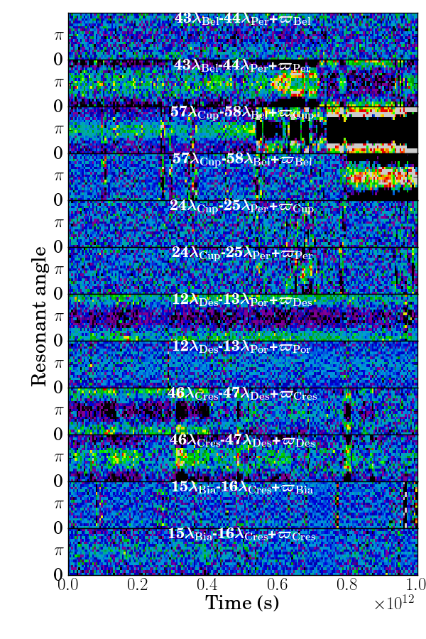
Figure 2: Histograms of resonant angles associated with first-order mean-motion resonances between two moons. The particular resonant angle plotted is labelled in each panel. When the color is black, the system spent no time with the resonant angle at that particular $y$ axis value. When the color is uniformly blue, the angle was evenly distributed and the angle was circulating.

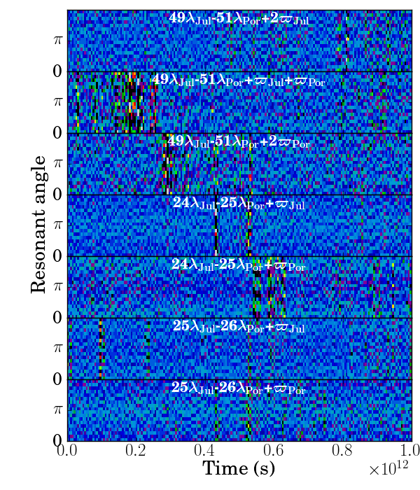
Figure 3: Histograms of resonant angles associated with first- and second-order mean-motion resonances between Juliet and Portia. The angle $24\lambda_{Jul}-25\lambda_{Por}+\varpi_{Por}$ spends more time at 0 and the angle $25\lambda_{Jul}-26\lambda_{Por}+\varpi_{Por}$ spends more time at $\pi$. Three histograms show angles associated with the 49:51 second-order mean-motion resonance between Juliet and Portia.

5.1 Two-body resonances between Uranian moons

In Table 3 we list computed properties of strong two-body first-order mean-motion resonances in the inner Uranian satellite system. We have computed characteristic libration frequencies for both resonance terms (that corresponding to $\phi_{qi}$ and that corresponding to $\phi_{qj}$) for the $i$-th and $j$-th body in a $q-1:q$ resonance and listed the maximum libration frequency

$$\nu_{max}\equiv\max(\nu_{i},\nu_{j},\nu_{ei},\nu_{ej}).$$ (64)

Here libration frequencies $\nu_{i},\nu_{j}$ are computed using equation 52 and $\nu_{ei},\nu_{ej}$ using equation 61. We use semi-major axes and eccentricities from the beginning of the integration to perform these computations. We identify which resonant term (that associated with $\phi_{qi}$ or $\phi_{qj}$) is larger from the maximum libration frequency and this is also listed in Table 3.

Libration frequencies for the strongest first-order mean-motion resonances are of order $10^{-7}$ Hz corresponding to periods of $10^{8}$s (a few years). By computing equation 62 from values for eccentricity and mass ratio listed in Table 1 and inter-satellite separations in Table 3, and restoring units by multiplying by the mean motion of the inner satellite (also listed in Table 1), we have checked that the approximation for the libration frequency (using equation 62) is within a factor of a few of the quantity more accurately calculated using Laplace coefficients.

In Table 3 we also list the ratio of eccentricity to critical eccentricity for the stronger resonant subterm

$$e_{m}\equiv\left\{\begin{array}[]{c}\frac{e_{i}}{e_{i,crit}}\\ \frac{e_{j}}{e_{j,crit}}\end{array}{\rm for}\begin{array}[]{c}\max(\nu_{i},\nu_{ei})\geq\max(\nu_{j},\nu_{ej})\\ \max(\nu_{i},\nu_{ei})<\max(\nu_{j},\nu_{ej})\end{array}\right.$$ (65)

and these are computed using equation 57. Distance to resonance is estimated with the frequency

$$b_{m}\equiv{\min(|b_{i}|,|b_{j}|)}.$$ (66)

When $b_{m}/\nu_{max}\la 1$ the pair of bodies is strongly influenced by the resonance. It will be helpful later on to consider $b_{m}$ as a small divisor when we discuss three-body resonances in section 7.1.

The coefficients $b_{i},b_{j}$ were computed using equation 46 and with precession rates calculated using equation 30 (and so lacking contribution from secular satellite interactions). We use equation 38 for $\epsilon_{i},\epsilon_{j}$ to compute quantities such as $\nu_{max}$ and $e_{m}$.

To compare the strengths of the $\phi_{qi}$ and $\phi_{qj}$ resonant terms we compute a ratio $\mu_{m}$

$$\mu_{m}\equiv\left\{\begin{array}[]{l}\mu_{ij}\\ \mu_{ij}^{-1}\end{array}\qquad{\rm for}\qquad\begin{array}[]{c}\mu_{ij}<1\\ \mu_{ij}>1\end{array}\right.$$ (71)

with

$$\mu_{ij}\equiv{\Gamma_{j}^{1\over 2}\epsilon_{j}\over\Gamma_{i}^{1\over 2}\epsilon_{j}}=\left({\nu_{ej}\over\nu_{ei}}\right)^{2}.$$ (72)

corresponding to coefficients in the Hamiltonian, equation 45. An energy for the dominant sub-term

$$\varepsilon_{m}\equiv\left\{\begin{array}[]{l}\epsilon_{i}\Gamma_{i}^{1\over 2}\\ \epsilon_{j}\Gamma_{j}^{1\over 2}\end{array}\right.\qquad{\rm for}\qquad\begin{array}[]{c}\mu_{ij}<1\\ \mu_{ij}>1\end{array}$$ (73)

is listed in Table 3 divided by the energy for the dominant term in the Cressida/Desdemona 46:47 resonance, denoted as $\varepsilon_{mCD}$. We also compute the frequency ratio

$$\lambda_{olp}\equiv\left|{\dot{\varpi}_{ij}\over\nu_{max}}\right|,$$ (74)

which is a parameter describing the proximity of the two resonance terms (Holman & Murray, 1996; Murray & Holman, 1997).

As can be seen from Table 3, and with the exception of resonances involving Cupid, at the beginning of the integration the bodies tend to be near but above the critical eccentricities for each resonance term. Thus usually $\nu_{ei}>\nu_{i}$ and $\nu_{ej}>\nu_{j}$. Cupid has a comparatively high eccentricity so $e_{m}>1$ for the 57:58 resonance with Belinda and the 24:25 resonance with Perdita.

Only for the Cupid/Belinda 57:58, Belinda/Perdita 43:44 and Cressida/Desdemona 46:47 resonances is the system clearly in the vicinity of resonance at the beginning of the integration with $b_{m}\la 1$. In the rightmost column in Table 3 we compute this energy divided by that for the Cressida/Desdemona 46:47 resonance, allowing a comparison of the relative energies of the resonant terms. The energy in the Juliet/Portia resonances is high because of the comparatively large masses of Juliet and Portia.

5.2 Intermittency in resonant angle histograms

Near a resonance, the resonant angle moves slowly or freezes. The distribution of angle values measured in a time interval peaks at the frozen angle and is not flat. Examination of histograms of a resonant angle during different time intervals is a way to search for resonant interaction in a numerical integration. For example, a pair of bodies with a resonant angle librating about $\pi$ has an angle histogram that is strongly peaked at $\pi$. If the pair of bodies are distant from the resonance, then the angle circulates and the histogram would be flat. Near a resonance separatrix, the histogram can peak at $\pi$ or 0 even if the angle circulates.

For each 500 data outputs (each spanning a time interval $5\times 10^{9}$s long) in the numerical integration, we used orbital elements, computed from the state vectors, to create histograms of the angles $\phi_{qi}$ and $\phi_{qj}$. These angles, modulo $2\pi$, are binned in 18 angular bins. The result is a two-dimensional histogram, with time intervals along one axis and angle along the other. Each bin counts the number of times the angle was in that angle bin during the time interval. We note that sometimes the sampling or data output period introduces structure into the histograms when the distribution should be flat. This happens when the angle plotted happens to have a period that is approximately an integer ratio of the sampling period. When there are variations in the period of the angle, then such aliasing is rarer. Unfortunately the integration output rate was not chosen with the creation of angle histograms in mind so we cannot decrease the output period or resample it.

The structure-exhibiting resonant angle histograms for first-order mean-motion resonance angles involving two bodies are shown in Figure 2 and Figure 3, with Figure 3 focusing on first- and second-order resonances between Juliet and Portia. In Figure 2 when the color is black, the system spent no time with the resonant angle in that particular bin. If the color is uniformly blue, then the angle was evenly distributed and was probably circulating. When the angle remains fixed or librates about a particular value there is a peak in the histogram at this $y$ axis value. The closest resonances, Cupid/Belinda 57:58, Belinda/Perdita 43:44 and Cressida/Desdemona 46:47 (at the top of Table 3 and with proximity measured as having a low value of $b_{m}/\nu_{max}$) have resonant angle histograms with particularly strong structure. These pairs spend more time with the resonant angle near 0 or $\pi$.

Even though Desdemona and Portia are not very near the 12:13 resonance (as seen from $b_{m}/\nu_{max}$ in Table 3), the resonant angle $12\lambda_{Des}-13\lambda_{Por}+\varpi_{Des}$ tends to remain near 0 and $12\lambda_{Des}-13\lambda_{Por}+\varpi_{Por}$ spends more time near $\pi$. Similarly $15\lambda_{Bia}-16\lambda_{Cres}+\varpi_{Cres}$ spends more time near $\pi$ than 0. Figure 3 shows that the 24:25 and 25:26 first-order resonances between Juliet and Portia could be important even though Juliet and Portia are nearer the weaker 49:51 second-order mean-motion resonance.

Intermittent behavior is seen in the resonant angle histograms of the 57:58 resonance of Cupid and Belinda, the 46:47 resonance of Cressida and Desdemona and the 43:44 resonance of Belinda and Perdita. The angle $57\lambda_{Cup}-58\lambda_{Bel}-\varpi_{Cup}$ librates about 0 or $\pi$, making transitions between the two states. Transitions between libration states are coupled in the Cupid, Belinda and Perdita trio. For example, when the angle $43\lambda_{Bel}-44\lambda_{Per}-\varpi_{Per}$ makes a transition from $\pi$ to 0 at $t\sim 8\times 10^{11}$s the angle $57\lambda_{Cup}-58\lambda_{Bel}-\varpi_{Bel}$ makes a transition from 0 to $\pi$. In contrast, Cressida and Desdemona’s resonant angles undergo a variety of transitions but none of the other two-body angles in Figure 2 make transitions at the same time.

We could view the transitions of the resonant angles as an example of ‘Hamiltonian intermittency’ (e.g., Shevchenko 2010). As discussed by Shevchenko (2010), Hamiltonian intermittency is attributed to oscillations in the location of a separatrix or sticky orbits (cantori) in the boundary of a chaotic layer. Perhaps both mechanisms are possible here. To investigate the source of chaotic behavior and associated intermittency we consider two possible sources of chaotic behavior. First, we consider the role of the two resonant terms in an individual first-order mean-motion resonance, following Holman & Murray (1996) who estimated Lyapunov timescales in mean-motion resonances in the asteroid belt based on overlap between resonant subterms. The Lyapunov exponents characterize the mean rate of exponential divergence of trajectories close to each other in the phase space. By Lyapunov timescale we mean the inverse of the maximum Lyapunov exponent. Second, in section 7 we will discuss the Lyapunov timescale in resonant chains, when there are pairs of first-order mean motions resonances in trios of bodies.

5.3 Resonance overlap between subterms in individual first-order resonances

If we can compare our Hamiltonian model to the well-studied non-linear driven pendulum then we can estimate the Lyapunov timescale in it. Because eccentricities are usually above or near the critical values we can assume that the system oscillates about a mean eccentricity value. In this case the coefficients of each resonant term are not strongly dependent upon the variations in the momenta $\Gamma_{i},\Gamma_{j}$. Using the strength ratio $\mu_{m}$, equation 45 can be approximately transformed (via canonical transformation) to

$$K(J,\phi;\Gamma,\varpi_{ij})\approx{A\over 2}J^{2}+b_{r}J+\Omega\Gamma\qquad\qquad\qquad\qquad$$ (75)

$$\qquad\qquad+\epsilon_{m}\left[\cos\phi+\mu_{m}\cos(\phi+\varpi_{ij})\right],$$

where $\phi$ is the angle $\phi_{i}$ or $\phi_{j}$ for the strongest term and is conjugate to $J$. The angle $\varpi_{ij}$ is conjugate to $\Gamma$ and $\Gamma$ is either $\Gamma_{i}$ or $\Gamma_{j}$ depending upon which resonant sub-term is dominant; likewise the coefficient $b_{r}$ is either $b_{i}$ or $b_{j}$. Here $\Omega$ is a perturbation frequency also representing the distance between the the two resonances; $\Omega\sim\pm\dot{\varpi}_{ij}$. The frequency of small oscillations for the dominant resonance $\nu_{max}=\sqrt{A\epsilon_{m}}$.

The Hamiltonian can be recognized as a periodically-perturbed pendulum (Chirikov, 1979; Shevchenko & Kouprianov, 2002; Shevchenko, 2014) and our description is equivalent to the forced-pendulum model for chaos in mean-motion resonances in the asteroid belt by Holman & Murray (1996); Murray & Holman (1997). The periodically-perturbed pendulum exhibits chaotic behavior in the separatrix of the primary resonance. Following Chirikov (1979); Shevchenko & Kouprianov (2002), a unitless overlap parameter, $\lambda_{olp}$, can be constructed from the perturbation frequency and frequency of small oscillations of the dominant resonance

$$\lambda_{olp}=\frac{\Omega}{\nu_{max}}=\frac{\dot{\varpi}_{ij}}{\nu_{max}}.$$ (76)

This parameter affects the separatrix width and the Lyapunov timescale inside the separatrix (Chirikov, 1979; Shevchenko & Kouprianov, 2002; Shevchenko, 2004, 2014). Whereas in the asteroid belt the separation between the two resonant subterms arises from secular interactions with giant planets, here the separation arises from the oblateness of the planet.

We can use an approximation for the precession rate (equation 31) and resonance libration frequencies (equation 55) for a closely-spaced system to estimate

$$\lambda_{olp}\sim 5.25\max(m_{i},m_{j})^{-\frac{2}{3}}\delta_{ij}^{\frac{7}{3}}j_{2}\left(\frac{R_{p}}{a_{i}}\right)^{2}$$ (77)

where we have set $q\sim\delta_{ij}^{-1}$ for the nearest first-order mean-motion resonance. The strong dependence on separation accounts for the differences in $\lambda_{olp}$ seen in Table 3.

Table 3 shows that the perturbation strengths of the sub-term, $\mu_{m}$, are not small, so the energy changes due to the perturbation term each orbit in the separatrix of the dominant resonance would be of order the energy in the resonance itself. However, inspection of Table 3 shows that the overlap ratio $\lambda_{olp}\la 0.1$ for most of the resonances. This puts them in the regime described as adiabatic chaos by Shevchenko (2008). In this regime, the Lyapunov timescale for chaotic evolution is approximately the perturbation period $T=2\pi/\Omega$ (logarithmically increasing only at very small $\lambda$, see equation 17 by Shevchenko (2008)). In units of the resonance libration period the Lyapunov timescale is approximately inversely proportion to $\lambda$. As the resonance libration periods are of order 1-10 years (frequencies are listed in Table 3), and the overlap parameters $\lambda_{olp}\la 0.1$, the Lyapunov timescale would be in the regime of 10-100 years. The overlap of these resonant subterms might account for some of the intermittency present in the resonant angles during the integration. We note that the separatrix width, in units of energy, depends on $\lambda_{olp}^{2}$ and is small when $\lambda_{olp}<1$ (the $W$ parameter $\propto\lambda_{olp}^{2}$; equation 5 of Shevchenko (2008), and the separatrix width is equal to this energy, see figure 1 of Shevchenko (2004)). Consequently the volume of phase space in which chaotic diffusion takes place is small in the adiabatic regime. Only for the more widely-spaced bodies is the overlap parameter in a regime giving a comparatively short Lyapunov timescale and a significant width in the chaotic region associated with the resonance separatrix.

Can we learn anything from considering what happens near a spherical planet or with $J_{2}=0$? Equation 77 implies that $\lambda_{olp}\to 0$ in this limit and we would expect integrable mean-motion resonances (and so no chaotic behavior). In contrast, Duncan & Lissauer (1997) found that an integration with $J_{2}=0$ exhibited more instability and had a shorter crossing timescale, opposite to what we expect. We have neglected the role of secular interaction terms between bodies, and when $J_{2}\to 0$ perhaps secular interactions between distant moons become more important.

The overlap of sub-terms in individual mean-motion resonances, particularly important for pairs of bodies that are not the nearest ones, could account for transitions of a single resonant angle from a state near 0 to $\pi$ and vice versa. However, this mechanism would not account for coupled variations in angles in pairs of bodies, or coupled variations in semi-major axis between more than two bodies. Since numerical integrations have shown that integration of fewer moons can increase the crossing timescale (French & Showalter, 2012), we are also interested in mechanisms involving additional moons for the intermittency in the resonant angles.

Table 3: Properties of strong first-order two-body resonances

(1)	(2)	(3)	(4)	(5)	(6)	(7)	(8)	(9)	(10)	(11)	(12)	(13)
$i$	$j$	q-1:q	$\delta_{ij}$	$\phi$	$\nu_{max}$(Hz)	$\frac{\nu_{max}}{n_{i}}$	$\frac{b_{m}}{\nu_{max}}$	$\frac{b_{m}}{n_{i}}$	$e_{m}$	$\lambda_{olp}$	$\mu_{\epsilon}$	$\frac{\varepsilon_{m}}{\varepsilon_{mCD}}$
Cressida	Desdemona	46:47	0.014	$\phi_{j}$	1.1e-07	6.9e-04	1.4	9.6e-04	0.89	0.065	1.28	1.00
Belinda	Perdita	43:44	0.015	$\phi_{j}$	2.1e-07	1.8e-03	0.1	1.3e-04	10.50	0.018	6.49	0.80
Cupid	Belinda	57:58	0.012	$\phi_{i}$	2.2e-07	1.8e-03	-2.4	-4.5e-03	5.51	0.013	0.09	-0.17
Desdemona	Portia	12:13	0.055	$\phi_{i}$	4.5e-08	3.0e-04	9.1	2.7e-03	0.29	0.508	0.36	-1.29
Bianca	Cressida	15:16	0.044	$\phi_{i}$	3.1e-08	1.8e-04	8.6	1.6e-03	2.37	0.748	0.55	-0.65
Rosalind	Perdita	7: 8	0.093	$\phi_{j}$	1.2e-08	9.1e-05	-20.7	-1.9e-03	7.38	2.083	4.78	0.08
Desdemona	Juliet	24:25	0.027	$\phi_{j}$	7.6e-08	4.9e-04	-29.8	-1.5e-02	3.80	0.160	0.54	3.73
Cressida	Juliet	16:17	0.042	$\phi_{j}$	4.4e-08	2.8e-04	62.7	1.8e-02	2.56	0.429	0.69	3.96
Cupid	Perdita	24:25	0.027	$\phi_{j}$	1.6e-08	1.3e-04	-93.9	-1.2e-02	67.58	0.424	0.58	0.00
Bianca	Desdemona	11:12	0.059	$\phi_{i}$	1.7e-08	9.9e-05	-92.9	-9.2e-03	2.60	1.818	0.70	-0.30
Portia	Rosalind	11:12	0.058	$\phi_{j}$	4.0e-08	2.8e-04	-95.3	-2.7e-02	0.41	0.505	2.78	1.87
Portia	Perdita	4: 5	0.156	$\phi_{j}$	1.6e-08	1.1e-04	-192.5	-2.1e-02	3.18	2.848	13.09	0.36
Rosalind	Cupid	10:11	0.064	$\phi_{j}$	1.4e-08	1.1e-04	-223.4	-2.3e-02	3.92	1.310	8.22	0.02
Portia	Cupid	5: 6	0.126	$\phi_{j}$	1.5e-08	1.1e-04	-227.2	-2.4e-02	1.63	2.541	22.66	0.07
Juliet	Cupid	4: 5	0.156	$\phi_{j}$	7.5e-09	5.1e-05	-440.5	-2.2e-02	2.03	6.548	14.97	0.03
Rosalind	Belinda	9:10	0.076	$\phi_{i}$	1.2e-08	9.0e-05	492.8	4.4e-02	0.67	1.785	0.74	-0.34
Portia	Belinda	5: 6	0.139	$\phi_{j}$	1.4e-08	9.8e-05	634.4	6.2e-02	0.28	2.947	2.04	1.29
Belinda	Perdita	42:43	0.015	$\phi_{j}$	2.0e-07	1.7e-03	-13.0	-2.3e-02	10.33	0.018	6.49	0.80
Belinda	Perdita	44:45	0.015	$\phi_{j}$	2.1e-07	1.8e-03	12.7	2.3e-02	10.68	0.018	6.49	0.79
Cressida	Desdemona	47:48	0.014	$\phi_{j}$	1.1e-07	6.9e-04	32.1	2.2e-02	0.91	0.064	1.28	1.00
Cressida	Desdemona	45:46	0.014	$\phi_{j}$	1.1e-07	6.8e-04	-30.0	-2.0e-02	0.88	0.066	1.28	1.00
Desdemona	Juliet	25:26	0.027	$\phi_{j}$	7.8e-08	5.1e-04	48.4	2.5e-02	3.92	0.154	0.54	3.70
Desdemona	Portia	11:12	0.055	$\phi_{i}$	4.3e-08	2.8e-04	-264.0	-7.4e-02	0.28	0.534	0.36	-1.30
Bianca	Cressida	14:15	0.044	$\phi_{i}$	2.9e-08	1.7e-04	-351.0	-6.1e-02	2.25	0.796	0.54	-0.66
Cressida	Juliet	15:16	0.042	$\phi_{j}$	4.2e-08	2.7e-04	-157.5	-4.2e-02	2.45	0.455	0.69	4.00
Cupid	Belinda	56:57	0.012	$\phi_{i}$	2.2e-07	1.8e-03	-11.9	-2.2e-02	5.44	0.014	0.09	-0.17
Cupid	Belinda	58:59	0.012	$\phi_{i}$	2.2e-07	1.9e-03	6.8	1.3e-02	5.58	0.013	0.09	-0.17
Portia	Rosalind	12:13	0.058	$\phi_{j}$	4.2e-08	2.9e-04	185.1	5.4e-02	0.44	0.483	2.79	1.85
Juliet	Portia	24:25	0.027	$\phi_{i}$	1.2e-07	8.2e-04	-22.6	-1.9e-02	1.30	0.091	0.67	-28.60
Juliet	Portia	25:26	0.027	$\phi_{i}$	1.2e-07	8.4e-04	24.8	2.1e-02	1.34	0.089	0.67	-28.38
Juliet	Portia	26:27	0.027	$\phi_{i}$	1.3e-07	8.5e-04	70.3	6.0e-02	1.38	0.087	0.67	-28.14
Rosalind	Belinda	8: 9	0.076	$\phi_{i}$	1.1e-08	8.4e-05	-715.2	-6.0e-02	0.62	1.907	0.74	-0.34
Desdemona	Rosalind	6: 7	0.116	$\phi_{j}$	5.6e-09	3.6e-05	1758.1	6.4e-02	0.85	7.760	1.00	0.13

The properties of strong first-order mean-motion resonances in the Uranian satellite system. Columns: 1,2 satellite names corresponding to bodies $i,j$. The resonant arguments are $\phi_{qi}=q\lambda_{j}+(1-q)\lambda_{i}-\varpi_{i}$ and $\phi_{qj}=q\lambda_{j}+(1-q)\lambda_{i}-\varpi_{j}$. Col 3: The integers $q-1:q$. Col 4: The spacing between the two bodies $\delta_{ij}$ computed using equation 18. Col 5: The dominant resonant argument (that with larger libration frequency) is denoted as $\phi_{i}$ if the $\phi_{qi}$ angle is important or $\phi_{j}$ if the $\phi_{qj}$ angle is important. Col 6: The frequency of librations in resonance, $\nu_{max}$, (equation 64) in units of Hz. This frequency is computed using equations 52,61) and 38. Col 7: $\nu_{max}$ divided by the innermost body’s mean motion, $n_{i}$. Col 8: The distance to resonance $b_{m}$ (equation 66) in units of $\nu_{max}$. When $|b_{m}/\nu_{max}|\la 1$ the system is near resonance. Here the frequencies $b_{i},b_{j}$ are computed using equation 46 and $b_{m}$, the distance to the dominant resonant argument. Col 9: The distance to resonance in units of the innermost body’s mean motion or the ratio $b_{m}/n_{i}$. Col 10: The ratio of initial eccentricity to critical eccentricity for the dominant argument (see equation 65, and this is computed using equation 57). Col 11: The unitless overlap ratio, $\lambda_{olp}$, (equation 74) describing the proximity of the $\phi_{qi}$ and $\phi_{qj}$ resonances. Col 12: The unitless parameter $\mu_{\epsilon}$, the ratio of $\phi_{qi}$ vs $\phi_{qj}$ resonance strengths (see equation 47). Col 13: Energy of the argument $\varepsilon_{m}$ (equation 73) divided by that for the Cressida/Desdemona 46:47 resonance. The resonances have been divided into two groups. For each satellite pair, the top set lists only the nearest first-order resonance. The bottom set includes more-distant resonances.

6 Three-body interactions

Overlap of three-body multiplets is a source of chaos in the asteroid belt (Nesvorný & Morbidelli, 1998a; Murray et al., 1998). Quillen (2011) proposed that three-body resonances were responsible for slow, chaotic diffusion in the semi-major axes of bodies in integrated planar closely-packed multiple-planet systems. Three-body resonances in the Uranian satellite system may account for some of the coupled variations we see between three or more bodies. To explore this possibility, we searched the inner Uranian satellite system for strong three-body resonances. When a three-body resonance is strong, the associated Laplace angle freezes or librates (Nesvorný & Morbidelli, 1998a, b; Smirnov & Shevchenko, 2013). We search for time periods when Laplace angles are slowly moving and then discuss comparisons between histograms of resonant angles and variations in orbital elements between trios of bodies.

6.1 Searching for nearby three-body resonances

The three-body resonances discussed by Quillen (2011) are specified by two integers $p,q$. The p:-(p+q):q resonance is associated with a Laplace angle

$$\theta=p\lambda_{i}-(p+q)\lambda_{j}+q\lambda_{k}$$ (78)

that involves mean longitudes of three bodies $i,j,k$ where we assume that the semi-major axes $a_{i}<a_{j}<a_{k}$. The Laplace angle is slowly moving when the frequency

$$\dot{\theta}\approx pn_{i}-(p+q)n_{j}+qn_{k}\sim 0$$ (79)

with $n_{i},n_{j},n_{k}$ the mean motions of the three bodies.

For trios of bodies, we searched for integers $p,q$ that minimized $|\dot{\theta}|$. For the trios Cressida, Juliet and Portia and Cressida, Desdemona and Portia we list three-body resonant angles, with $|\dot{\theta}|<6\times 10^{7}$ Hz at some time in the interval $t=0$–$10^{12}$s, in Table 4, and we plot histograms of these resonant angles in Figures 4 and 5. We limited our search to $p,q<100$ as Laplace coefficients (and so resonant strengths) are truncated exponentially with $p\delta_{ij}>1$ or $q\delta_{jk}>1$, with $\delta_{ij},\delta_{jk}$ describing the distances between the moons (Quillen 2011, and as shown in equation 22).

Gravitational interactions only involve two bodies, and it is only via canonical transformation that we derive a Hamiltonian that contains a three-body Laplace angle. Quillen (2011) estimated three-body resonance strengths assuming that the dominant contribution was from two zeroth-order (in eccentricity) perturbation terms,

$$W_{ij,p}\cos p(\lambda_{i}-\lambda_{j})+W_{ij,q}\cos q(\lambda_{j}-\lambda_{k}),$$ (80)

that are Fourier components of two-body interaction terms. A near-identity canonical transformation gives a Hamiltonian in the vicinity of three-body resonance lacking these two terms

$$H(\vec{\Lambda},\vec{\lambda})=\sum_{l=i,j,k}-\frac{m_{l}^{3}}{2\Lambda_{i}^{2}}\\ +\epsilon_{pq}\cos(p\lambda_{i}-(p+q)\lambda_{j}+q\lambda_{k}).$$ (81)

The coefficient $\epsilon_{pq}(\vec{\Lambda})$ is sensitive to divisors $n_{ij}$ and $n_{jk}$ that are the difference in mean motions of the two bodies (see equation 23 for $\epsilon_{pq}$ of Quillen 2011) and can be considered a second-order perturbation (and depending on a higher power of moon mass) as it involves a product of the coefficients $W_{ij,p}$ and $W_{jk,q}$. The dependence on divisors $n_{ij}$ and $n_{jk}$ suggests that all the resonances listed in Table 4 should have similar strengths. However, we can see by comparing the resonant angle histograms in Figures 4 and 5 that this is probably not the case.

We first check to see if the resonant angles freeze only if the three bodies are very near resonance. For the Cressida, Juliet and Portia trio there is a time when the bodies are very near the 29:-76:47 resonance (with $|\dot{\theta}|<10^{-10}$ Hz, as listed in Table 4). Most of the other resonances have minimum distance $|\dot{\theta}|\sim 10^{-7}$ Hz. Despite proximity to resonance, the 29:-76:47 resonant angle does not show more structure than the other angles in Figure 4. The Cressida, Desdemona and Portia trio is near both the 39:-50:11 and 46:-59:13 resonances but only the 46:-59:13 resonant angle shows strong structure in Figure 5. We find that proximity is not the only factor governing three-body resonant strength (as inferred through structure in a resonant angle histogram).

As discussed in section 5, Cressida and Desdemona are near or in the 46:47 first-order mean-motion resonance and Desdemona and Portia are near their 12:13 first-order mean-motion resonance. The two resonant angles from the nearby first-order mean-motion resonances are

$$\phi_{p} = 47\lambda_{Des}-46\lambda_{Cres}-\varpi_{Des}$$

$$\phi_{q} = 13\lambda_{Por}-12\lambda_{Des}-\varpi_{Des}$$

and the difference between these angles

$$\theta = \phi_{q}-\phi_{p}$$ (82)

$$= 46\lambda_{Cres}-59\lambda_{Des}+13\lambda_{Por}$$

and equivalent to the 46:-59:13 Laplace angle involving the three bodies Cressida, Desdemona and Portia. This particular three-body resonance could be strong because each consecutive pair of bodies is near a first-order mean-motion resonance. We describe this setting as a ‘resonant chain’. The 39:-50:11 three-body resonance, perhaps because it is not near any first-order mean-motion resonances between pairs of bodies, is weaker than the 46:-59:13 resonance. In Figure 5 the 92:-118:26 angle histogram also shows structure, however this angle is a multiple of two of the 46:-59:13 Laplace angle. The 92:-118:26 Laplace angle histogram may show structure due to the 46:-59:13 three-body resonance.

In Figure 4 the 5:-13:8 angle histogram shows structure suggesting that this resonance with Cressida, Juliet and Portia might be stronger than the other three-body resonances in this trio. If Cressida, Juliet and Portia are near the 5:-13:8 resonance then they are also near resonances described with integer multiples of this, the 10:-25:16 (multiply by 2) and the 15:-39:24 (multiply by 3) resonances. For resonance strengths estimated from the zeroth-order interaction terms alone, the resonance strength energy coefficient $\epsilon_{pq}\sim\epsilon_{2p,2q}$ and so on for other multiples as long as the strength is not exponentially truncated by the Laplace coefficients. The 5:-13:8 three-body resonance may be strong because of the contribution from higher-index multiples.

Is the 5:-13:8 resonance with Cressida, Juliet and Portia also near two two-body first-order resonances and a Laplace angle associated with a resonant chain? As seen in Table 3 Cressida and Juliet are fairly near the 15:16 first-order resonance and Juliet and Portia fairly near the 23:24 first-order resonance. The 15:-39:24 Laplace angle is a multiple of 3 times the 5:-13:8 Laplace angle. The 5:-13:8 Laplace angle may show structure due to the 15:16 resonance between Cressida and Juliet or the 23:24 resonance between Juliet and Portia. The histogram on the lower right in Figure 4 shows the the histogram for the Laplace angle 15:-39:24 with $\dot{\theta}=1.8\times 10^{-6}$ Hz, and this angle shows structure even though the distance to resonance is larger than the other considered Laplace angles. The structure in the 5:-13:8 Cressida, Juliet and Portia angle histogram could be explained by the combined effects of the 5:-13:8 and multiples of this resonance, each with strength contributed with zeroth-order terms, or because the 15:-39:24 resonance is near a chain of first-order resonances.

Table 4: Potential three-body resonances

Cres/Jul/Por		Cres/Des/Por
$p$:-($p$+$q$):$q$	$\dot{\theta}$(Hz)	$p$:-($p$+$q$):$q$	$\dot{\theta}$(Hz)
5:-13:8	6.0e-07	7:-9:2	-2.4e-07
8:-21:13	-1.2e-07	14:-18:4	-4.8e-07
13:-34:21	3.9e-07	25:-32:7	5.3e-07
16:-42:26	-2.3e-07	32:-41:9	2.0e-07
21:-55:34	1.9e-07	39:-50:11	-1.8e-10
24:-63:39	-3.5e-07	46:-59:13	-7.9e-11
29:-76:47	-5.4e-11	53:-68:15	-1.3e-07
32:-84:52	-4.7e-07	60:-77:17	-3.7e-07
34:-89:55	5.8e-07	64:-82:18	4.0e-07
37:-97:60	-4.0e-11	71:-91:20	7.5e-08
40:-105:65	-5.8e-07	78:-100:22	-3.6e-10
42:-110:68	3.8e-07	85:-109:24	8.9e-11
45:-118:73	-2.4e-10	92:-118:26	-1.6e-10
50:-131:81	1.8e-07	99:-127:28	-2.7e-08
53:-139:86	-4.7e-08
58:-152:94	-1.1e-10
61:-160:99	-1.6e-07

The first and third columns list $p$:-($p$+$q$):$q$ with $p,q<100$, such that the frequency $\dot{\theta}=pn_{i}-(p+q)n_{j}+qn_{k}$ has $|\dot{\theta}|<6\times 10^{7}$ Hz at some time in the integration with $t<10^{12}$s. The second and fourth columns list $\dot{\theta}$ in Hz. The three bodies are Cressida, Juliet and Portia for the left two columns and Cressida, Desdemona and Portia for the right two columns. Histograms of the resonant angles are shown in Figures 4 and 5.

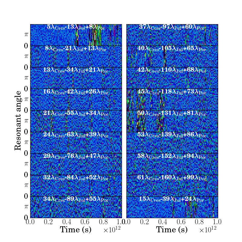
Figure 4: Histograms of resonant angles of nearby three-body resonances for Cressida, Juliet and Portia. The resonant angle plotted is labelled in each panel.

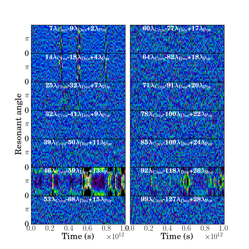
Figure 5: Histograms of resonant angles of nearby three-body resonances Cressida, Desdemona and Portia.

6.2 Comparing variations in angle histograms with variations in orbital elements

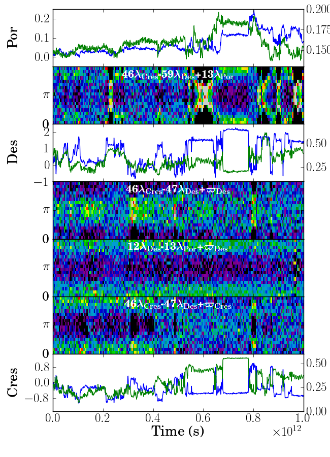
Figure 6: Two- and three-body resonances influencing Cressida, Desdemona and Portia. We plot both resonant angles (as histograms), semi-major axes (blue lines) and eccentricities (green lines) so that they can be directly compared. Scaling for semi-major axes and eccentricities is the same as in Figure 1. Transitions in the 46:-59:13 Laplace angle with Cressida, Desdemona and Portia are coincident with coupled variations in semi-major axes of the three moons.

To explore the role of three-body angles we compare the structure seen in histograms of two-body and three-body resonant angles with variations in orbital elements. The strongest structure seen in the histogram of a Laplace angle was that seen in the 46:-59:13 angle with Cressida, Desdemona and Portia. We plot in Figure 6 the 46:-59:13 Laplace angle histogram, the resonant angle histograms for the 46:47 first-order resonance between Cressida and Desdemona, the 12:13 resonance between Desdemona and Portia and semi-major axes and eccentricities for the three bodies as a function of time. We find that transitions between states in the three-body resonant angle are simultaneous with variations in semi-major axis in all three bodies. The transitions in the three-body resonant angles are more important than those seen in the two-body resonant angles. For example, at $t\sim 3.5\times 10^{11}$s the angle $46\lambda_{Cres}-47\lambda_{Des}+\varpi_{Cres}$ flips from 0 to $\pi$ and there are only weak variations in $a_{Cres},a_{Des}$ at this time. However at $t\sim 4\times 10^{11}$s the Laplace angle $46\lambda_{Cres}-47\lambda_{Des}+13\lambda_{Cres}$ varies from 0 to $\pi$ and coupled variations in semi-major axis of all three bodies are seen. Cressida and Portia move inward as Desdemona moves outward, as predicted from conserved quantities present when a three-body resonance is important (Quillen, 2011). Transitions of the Laplace angle are better associated with jumps in semi-major axis of all three bodies than the transitions in the two-body resonant angles.

Coupled motions in the semi-major axes of three bodies arise from a Hamiltonian that contains a three-body Laplace angle. Using Hamilton’s equation on equation 81

$$\dot{\Lambda}_{i}=-\frac{\partial H}{\partial\lambda_{i}}=p\epsilon_{pq}\sin(p\lambda_{i}-(p+q)\lambda_{j}+q\lambda_{k}).$$ (83)

If the Laplace angle is quickly circulating then on average $\Lambda_{i}$ (the Poincaré coordinate dependent on $a_{i}$) does not change. However if the Laplace angle remains fixed at $\pi/2$ then $\Lambda_{i}$ can increase or decrease, depending on the sign of $\epsilon_{pq}$. By similarly computing $\dot{\Lambda}_{j}$ and $\dot{\Lambda}_{k}$ we find that simultaneous variation in the semi-major axis of the three bodies would take place with the inner and outer bodies moving together and the middle one moving in the opposite direction.

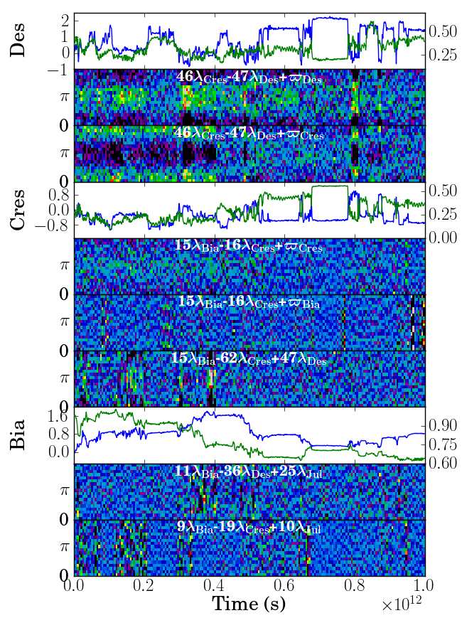
Figure 7: Two- and three-body resonances influencing Bianca, Cressida and Desdemona. We plot both resonant angles (histograms), semi-major axes (blue lines) and eccentricities (green lines) so that they can be directly compared. Scaling for semi-major axes and eccentricities is the same as in Figure 1. Variations in the semi-major axis of Bianca tend to happen during transitions in three-body Laplace angles.

In Figure 7 we plot resonant angles and orbital elements with the goal of understanding the variations in Bianca’s orbit. A three-body resonance influencing Bianca appears to be the 15:-62:47 between Bianca, Cressida and Desdemona; it is in proximity to the 15:16 first-order mean-motion resonance between Bianca and Cressida and the 46:47 first-order mean-motion resonance between Cressida and Desdemona. This is a resonant chain. The 11:-36:25 resonance between Bianca, Desdemona and Juliet maybe responsible for variations in Bianca’s orbital elements at $t\sim 3.5-5\times 10^{11}$s. This is near the 11:12 first-order mean-motion resonance between Bianca and Desdemona and the 24:25 first-order mean-motion resonance between Desdemona and Juliet, so it too is a resonant chain. The 9:-19:10 resonance between Bianca, Cressida and Juliet is not near any two-body resonances, and neither is it a multiple of the Laplace angle of a resonant chain. Since it has low $p,q$ it may be strong because resonances associated with multiples of the resonant angle contribute to its strength. Most of the variations in Bianca’s semi-major axis are correlated with periods of time where three-body Laplace angles are slowly moving or undergoing transitions.

In Figure 8 we show additional angle histograms linking motions of Desdemona, Juliet, Portia and Rosalind. Not all variations in orbital elements are explained. For example, Rosalind drops in eccentricity at $t\sim 8.5\times 10^{11}$s without any strong change in semi-major axis. This could be due to a secular resonance that we have not identified. A small jump in Rosalind’s semi-major axis at $t\sim 4\times 10^{11}$s is most likely due to a Desdemona, Juliet and Rosalind coupling such as the 20:-27:7 resonance as Desdemona and Rosalind both move outwards while Juliet moves inward. The 20:-27:7 resonance of Desdemona, Juliet and Rosalind is a resonant chain but not with consecutive pairs; rather, the chain involves the 6:7 first-order resonance between Desdemona and Rosalind (the outer two bodies) and the 20:21 between Desdemona and Juliet. Juliet, Portia and Rosalind are near a 2:-3:1 Laplace resonance that could be strong because many of its multiples would contribute to the resonance.

In Figure 9 we examine variations in Cupid, Belinda and Perdita. The two-body first-order resonances, the 57:58 between Cupid and Belinda, the 24:25 between Cupid and Perdita and the 43:44 between Belinda and Perdita account for many of the variations in orbital elements. However, a number of three-body angles show structure. The 7:-43:36 Laplace angle between Rosalind, Belinda and Perdita is a sum of the 43:44 resonant angle with Belinda/Perdita and the 7:8 resonant angle between Rosalind/Perdita, so it is a resonant chain but involving a mean-motion resonance with the outer pair Rosalind/Perdita. Rosalind, Belinda and Perdita are near a low-integer 2:-3:1 Laplace resonance and Rosalind, Cupid and Perdita are near a 4:-7:5 Laplace resonance, and these could be strong because many of their multiples would contribute to the resonance. The 5:-61:56 with Portia, Cupid and Belinda is a chain with the 5:6 between Portia and Cupid and the 55:56 resonance with Cupid and Belinda. Likewise the 4:-61:57 with Juliet, Cupid and Belinda is a resonant chain (the 4:5 with Juliet/Cupid and the 56:57 with Cupid/Belinda). Cupid and Belinda are so near each other that the 55:56 resonance is nearby even though the nearest resonance is the 57:58. The three-body resonances involving Juliet and Portia perhaps account for the sensitivity of Cupid’s crossing timescale to the presence of bodies other than Belinda and Perdita (French & Showalter, 2012).

In Figures 8 and 9 we found histograms of Laplace angles exhibiting structure, and they are resonant chains, but instead of involving mean motions between consecutive pairs, they involve a mean-motion resonance between the inner and outer body of the trio. There are two ways to create the three-body $p:-(p+q):q$ Laplace angle from a difference of first-order resonance arguments involving pairs of bodies,

$$\theta=(p+q-1)\lambda_{i}-(p+q)\lambda_{j}+\varpi_{i}\\ -\left[(q-1)\lambda_{i}-q\lambda_{k}+\varpi_{i}\right]$$ (84)

for the $(p+q-1):(p+q)$ resonances between bodies $i,j$ and the $(q-1):q$ resonance between bodies $i,k$ and

$$\theta=p\lambda_{i}-(p+1)\lambda_{k}+\varpi_{k}\\ -\left[(p+q)\lambda_{j}-(p+q+1)\lambda_{k}+\varpi_{k}\right]$$ (85)

for the $p:(p+1)$ resonance between bodies $i,k$ and the $(p+q):(p+q+1)$ resonance between bodies $j,k$. The 20:-27:7 resonance with Desdemona, Juliet and Rosalind is an example of that in equation 84 and the 7:-43:36 Laplace angle between Rosalind, Belinda and Perdita is an example of that in equation 85.

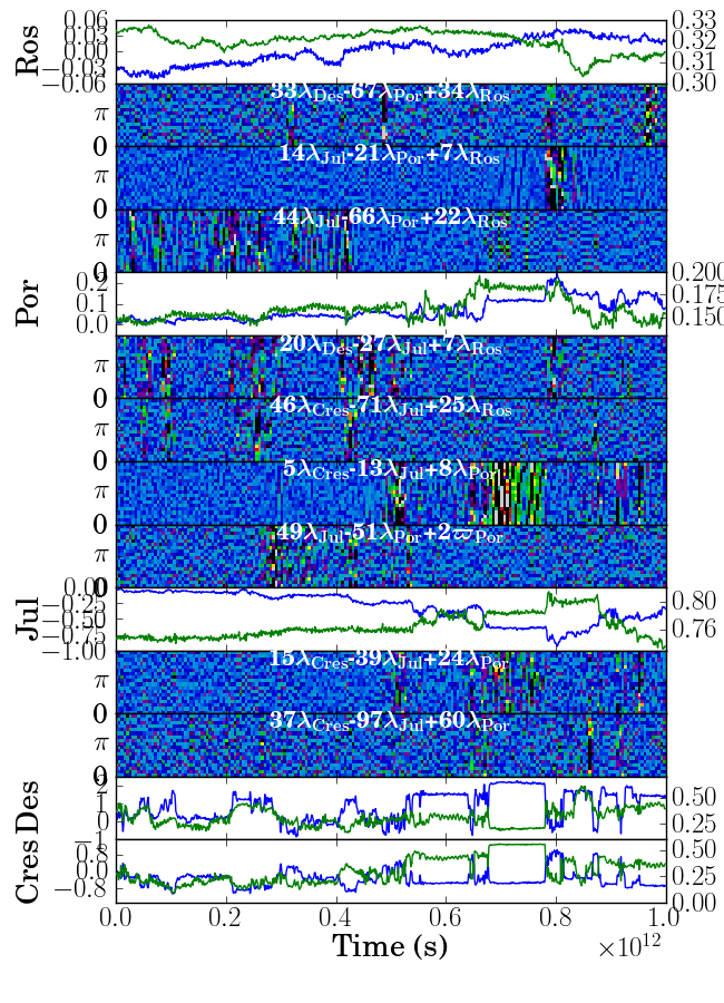
Figure 8: Two- and three-body resonances influencing Desdemona, Juliet, Portia and Rosalind. We plot both resonant angles (histograms), semi-major axes (blue lines) and eccentricities (green lines) so that they can be directly compared. Scaling for semi-major axes and eccentricities is the same as in Figure 1.

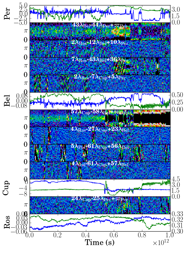
Figure 9: Two- and three-body resonances influencing Rosalind, Cupid, Belinda and Perdita. We plot both resonant angles (histograms), semi-major axes (blue lines) and eccentricities (green lines) so that they can be directly compared. Scaling for semi-major axes and eccentricities is the same as in Figure 1. The 57:58 Cupid/Belinda and 24:25 Cupid/Perdita two-body resonances account for many of the variations in orbital elements. The presence of three-body resonances involving Portia or Juliet with Cupid may account for the sensitivity of Cupid’s crossing timescale to the presence of these bodies.

7 Three-body resonant strengths and chaotic behavior near a resonant chain of two first-order mean-motion resonances

From the Laplace angle histograms, we have identified candidate three-body resonances in the Uranian system. While many of the variations in orbital elements in the Cupid, Belinda and Perdita trio appear to be caused by a trio of two-body resonances, three-body resonances seem particularly important amongst the Bianca, Cressida, Desdemona, Juliet and Portia group. In section 7.1 we calculate, using a near-identity canonical transformation, three-body resonance strengths for the setting where a trio of bodies is near (but not extremely close to) a pair of two-body first-order mean-motion resonances. Three-body resonance strengths and their libration frequencies are computed for the strong three-body resonances previously identified in the Uranian satellite system.

When a two-body resonant angle freezes, this gives a small divisor in the near-identity canonical transformation used in section 7.1, so in section 7.3 we employ a different canonical transformation for a Hamiltonian containing two first-order resonant terms. The resulting Hamiltonian resembles a forced pendulum and is used to estimate Lyapunov timescales from resonant overlap in the setting when a trio of bodies is in a resonant chain of two first-order resonances.

7.1 Resonant strengths of three-body resonances near two-body first-order mean-motion resonances

Quillen (2011) ignored the effect of nearby two-body resonances when estimating the strength of a three-body resonance. However, Figures 4 and 5 suggest that these are stronger than three-body resonances that are distant from two-body resonances. To estimate the strength of resonant-chain three-body resonances we follow a similar procedure to that used by Quillen (2011), using a first-order (in perturbation strengths) near-identity canonical transformation. However, instead of using zeroth-order perturbation terms (in eccentricity) we use first-order (in eccentricity) perturbation terms. Here we consider the case when the system is near, but not in, either two-body resonance so that small divisors do not invalidate the first-order nature of the transformation.

We consider the Keplerian Hamiltonian, precession terms due to the oblate planet and two first-order (in eccentricity) resonance terms

$$H(\vec{\Lambda},\vec{\Gamma},\vec{\lambda},\vec{\gamma})=\sum_{l}\left[-\frac{m_{l}^{3}}{2\Lambda_{l}^{2}}+B_{l}\Gamma_{l}\right]\\ \epsilon_{p}\Gamma_{j}^{\frac{1}{2}}\cos(p\lambda_{j}+(1-p)\lambda_{i}-\varpi_{j})\\ +\epsilon_{q}\Gamma_{j}^{\frac{1}{2}}\cos(q\lambda_{k}+(1-q)\lambda_{j}-\varpi_{j})$$ (86)

with

$$\epsilon_{p}(\Lambda_{i},\Lambda_{j}) = -\frac{m_{i}m_{j}^{3}}{\Lambda_{j}^{2}}\left(\frac{2}{\Lambda_{j}}\right)^{\frac{1}{2}}f_{31}(\alpha_{ij},p)$$

$$= -\frac{m_{i}m_{j}^{\frac{1}{2}}2^{\frac{1}{2}}}{a_{j}^{\frac{5}{4}}}f_{31}(\alpha_{ij},p)$$

$$\epsilon_{q}(\Lambda_{j},\Lambda_{k}) = -\frac{m_{j}m_{k}^{3}}{\Lambda_{k}^{2}}\left(\frac{2}{\Lambda_{j}}\right)^{\frac{1}{2}}f_{27}(\alpha_{jk},q)$$ (87)

$$= -\frac{m_{j}^{\frac{1}{2}}m_{k}2^{\frac{1}{2}}}{a_{k}a_{j}^{\frac{1}{4}}}f_{27}(\alpha_{ij},p)$$

using equations LABEL:eqn:Vij and 38 for the coefficients for the two-body first-order mean-motion resonances. We define angles

$$\phi_{p} \equiv p\lambda_{j}+(1-p)\lambda_{i}-\varpi_{j}$$

$$\phi_{q} \equiv q\lambda_{k}+(1-q)\lambda_{j}-\varpi_{j}.$$ (88)

We have chosen two resonant angles that contain $\varpi_{j}$. The Hamiltonian contains two terms that are first order in perturbation parameters $\epsilon_{p},\epsilon_{q}$.

Using a canonical transformation first order in perturbation strengths, we try to remove the two resonant terms. The result is a Hamiltonian that contains no first-order terms but does contain second-order terms proportional to $\epsilon_{p}\epsilon_{q}$. We use a generating function that is a function of new momenta ($\vec{\Lambda}^{\prime},\vec{\Gamma}^{\prime}$) and old angles ($\vec{\lambda},\vec{\gamma}$)

$$F_{2}(\vec{\Lambda}^{\prime},\vec{\Gamma}^{\prime};\vec{\lambda},\vec{\gamma})=\sum_{l}\left[\Lambda_{l}^{\prime}\lambda_{l}+\Gamma_{l}^{\prime}\gamma_{l}\right]\\ -\frac{\epsilon_{p}\Gamma{{}^{\prime}}_{j}^{\frac{1}{2}}}{\dot{\phi}_{p}}\sin\phi_{p}-\frac{\epsilon_{q}\Gamma{{}^{\prime}}_{j}^{\frac{1}{2}}}{\dot{\phi}_{q}}\sin\phi_{q}$$ (89)

with divisors

$$\dot{\phi}_{p} \equiv pn_{j}+(1-p)n_{i}+B_{j}$$

$$\dot{\phi}_{q} \equiv qn_{k}+(1-q)n_{j}+B_{j}$$ (90)

and with $B_{j}$ from secular perturbations. The mean motions, $B_{j}$, $\epsilon_{p}$ and $\epsilon_{q}$ are evaluated using momenta $\vec{\Lambda}^{\prime}$ . Near a two-body resonance $\dot{\phi}_{p}$ or $\dot{\phi}_{q}$ is small, leading to a strong perturbation or a small divisor. We assume here that the system is near but not exactly on resonance so these divisors never actually reach zero. Equivalently we assume that the angles $\phi_{p},\phi_{q}$ are circulating, increase or decrease continually, and do not librate around a particular value or remain fixed. In the next section we will employ a different change of variables that contains no small divisors.

The canonical transformation gives a near-identity transformation. New coordinates are equivalent to old coordinates plus a term that is first order in perturbation strengths $\epsilon_{p}$ or $\epsilon_{q}$. Relations between new and old coordinates are

$$\Lambda_{i} = \frac{\partial F_{2}}{\partial\lambda_{i}}=\Lambda_{i}^{\prime}-(1-p)\frac{\epsilon_{p}}{\dot{\phi}_{p}}\Gamma{{}^{\prime}}_{j}^{\frac{1}{2}}\cos\phi_{p}$$

$$\Lambda_{j} = \frac{\partial F_{2}}{\partial\lambda_{j}}=\Lambda_{j}^{\prime}-p\frac{\epsilon_{p}}{\dot{\phi}_{p}}\Gamma{{}^{\prime}}_{j}^{\frac{1}{2}}\cos\phi_{p}-(1-q)\frac{\epsilon_{q}}{\dot{\phi}_{q}}\Gamma{{}^{\prime}}_{j}^{\frac{1}{2}}\cos\phi_{q}$$

$$\Lambda_{k} = \frac{\partial F_{2}}{\partial\lambda_{k}}=\Lambda_{k}^{\prime}-q\frac{\epsilon_{q}}{\dot{\phi}_{q}}\Gamma{{}^{\prime}}_{j}^{\frac{1}{2}}\cos\phi_{q}$$

$$\lambda_{i}^{\prime} = \frac{\partial F_{2}}{\partial\Lambda_{i}^{\prime}}=\lambda_{i}+\left[\frac{\epsilon_{p}}{\dot{\phi}_{p}}\frac{\partial\dot{\phi}_{p}}{\partial\Lambda_{i}}-\frac{\partial\epsilon_{p}}{\partial\Lambda_{i}}\right]\frac{\Gamma{{}^{\prime}}_{j}^{\frac{1}{2}}}{\dot{\phi}_{p}}\sin\phi_{p}$$

$$\lambda_{j}^{\prime} = \frac{\partial F_{2}}{\partial\Lambda_{j}^{\prime}}=\lambda_{j}+\left[\frac{\epsilon_{p}}{\dot{\phi}_{p}}\frac{\partial\dot{\phi}_{p}}{\partial\Lambda_{j}}-\frac{\partial\epsilon_{p}}{\partial\Lambda_{j}}\right]\frac{\Gamma{{}^{\prime}}_{j}^{\frac{1}{2}}}{\dot{\phi}_{p}}\sin\phi_{p}$$

$$+\left[\frac{\epsilon_{q}}{\dot{\phi}_{q}}\frac{\partial\dot{\phi}_{q}}{\partial\Lambda_{j}}-\frac{\partial\epsilon_{q}}{\partial\Lambda_{j}}\right]\frac{\Gamma{{}^{\prime}}_{j}^{\frac{1}{2}}}{\dot{\phi}_{q}}\sin\phi_{q}$$

$$\lambda_{k}^{\prime} = \frac{\partial F_{2}}{\partial\Lambda_{k}^{\prime}}=\lambda_{k}+\left[\frac{\epsilon_{q}}{\dot{\phi}_{q}}\frac{\partial\dot{\phi}_{q}}{\partial\Lambda_{k}}-\frac{\partial\epsilon_{q}}{\partial\Lambda_{k}}\right]\frac{\Gamma{{}^{\prime}}_{j}^{\frac{1}{2}}}{\dot{\phi}_{q}}\sin\phi_{q}.$$

$$\gamma_{i}^{\prime} = -\varpi_{i}^{\prime}=\frac{\partial F_{2}}{\partial\Gamma{{}^{\prime}}_{i}}=\gamma_{i}=-\varpi_{i}$$

$$\gamma_{j}^{\prime} = -\varpi_{j}^{\prime}=\frac{\partial F_{2}}{\partial\Gamma{{}^{\prime}}_{j}}=-\varpi_{j}-\frac{\epsilon_{p}}{2\Gamma{{}^{\prime}}_{j}^{\frac{1}{2}}\dot{\phi}_{p}}\sin\phi_{p}-\frac{\epsilon_{q}}{2\Gamma{{}^{\prime}}_{j}^{\frac{1}{2}}\dot{\phi}_{q}}\sin\phi_{q}$$

$$\gamma_{i}^{\prime} = \frac{\partial F_{2}}{\partial\Gamma{{}^{\prime}}_{k}}=\gamma_{k}=-\varpi_{k}$$

$$\Gamma_{i} = \frac{\partial F_{2}}{\partial\gamma_{i}}=\Gamma_{i}^{\prime}$$

$$\Gamma_{j} = \frac{\partial F_{2}}{\partial\gamma_{j}}=\Gamma_{j}^{\prime}-\frac{\epsilon_{p}}{\dot{\phi}_{p}}\Gamma{{}^{\prime}}_{j}^{\frac{1}{2}}\cos\phi_{p}-\frac{\epsilon_{p}}{\dot{\phi}_{q}}\Gamma{{}^{\prime}}_{j}^{\frac{1}{2}}\cos\phi_{q}$$

$$\Gamma_{k} = \frac{\partial F_{2}}{\partial\gamma_{k}}=\Gamma_{k}^{\prime}$$

Inserting the new variables into the Hamiltonian (equation 86) we expand to second order in perturbation strengths $\epsilon_{p}$ and $\epsilon_{q}$. We neglect terms proportional to $\cos^{2}\phi_{p}$ or $\sin^{2}\phi_{p}$ (and similarly for $\phi_{q}$) and keep terms proportional to $\cos\phi_{p}\cos\phi_{q}$ and $\sin\phi_{p}\sin\phi_{q}$. We rewrite these products in terms of the Laplace angle

$$\theta\equiv\phi_{q}-\phi_{p}=(p-1)\lambda_{i}-(p-1+q)\lambda_{j}+q\lambda_{k}$$ (92)

that is similar to that discussed in the previous section where we discussed a search for nearby three-body resonances (see equation 78 but with $p-1$ replacing $p$).

Neglecting the primes on the coordinates, the Hamiltonian (equation 86) in the new variables is

$$K(\vec{\Lambda},\vec{\Gamma},\vec{\lambda},\vec{\gamma})=\sum_{l}\left[-\frac{m_{l}^{3}}{2\Lambda_{l}^{2}}+B_{l}\Gamma_{l}\right]\\ +\chi_{pq}\cos((p-1)\lambda_{i}-(p+q-1)\lambda_{j}+q\lambda_{k}).$$ (93)

The first-order terms (proportional to $\epsilon_{p}$ or $\epsilon_{q}$) have been removed leaving a single three-body term that is second order in perturbation strengths and proportional to $\epsilon_{p}\epsilon_{q}$. The three-body term has coefficient

$$\chi_{pq}=-\frac{3}{2}\frac{p(1-q)\Gamma_{j}}{m_{j}a_{j}^{2}}\frac{\epsilon_{p}\epsilon_{q}}{\dot{\phi}_{p}\dot{\phi}_{q}}\\ +(q-1)\frac{\epsilon_{q}\Gamma_{j}}{2\dot{\phi}_{p}}\left(\frac{\epsilon_{p}}{\dot{\phi}_{p}}\frac{\partial\dot{\phi}_{p}}{\partial\Lambda_{j}}-\frac{\partial\epsilon_{p}}{\partial\Lambda_{j}}\right)\\ -p\frac{\epsilon_{p}\Gamma_{j}}{2\dot{\phi}_{p}}\left(\frac{\epsilon_{q}}{\dot{\phi}_{q}}\frac{\partial\dot{\phi}_{q}}{\partial\Lambda_{j}}-\frac{\partial\epsilon_{q}}{\partial\Lambda_{j}}\right)\\ -\frac{p\epsilon_{p}\Gamma_{j}}{2\dot{\phi}_{p}}\frac{\partial\epsilon_{q}}{\partial\Lambda_{j}}+\frac{(q-1)\epsilon_{q}\Gamma_{j}}{2\dot{\phi}_{q}}\frac{\partial\epsilon_{p}}{\partial\Lambda_{j}}\\ -\frac{\epsilon_{q}\epsilon_{p}}{2}\left(\frac{1}{\dot{\phi}_{p}}+\frac{1}{\dot{\phi}_{q}}\right).$$ (94)

The first term arises from the Keplerian part of the Hamiltonian, the remainder from the resonant terms. The second and third terms come through perturbations on mean longitudes, the fourth and fifth terms through perturbations on $\Lambda$, and the last term from perturbations on $\varpi_{j}$ and $\Gamma_{j}$. Neglecting the dependence of precession rates on $\Lambda_{j}$,

$$\frac{\partial\dot{\phi}_{p}}{\partial\Lambda_{j}} \approx (p-1)\frac{3n_{j}}{\Lambda_{j}}=\frac{3(p-1)}{m_{j}a_{j}^{2}}$$ (95)

$$\frac{\partial\dot{\phi}_{q}}{\partial\Lambda_{j}} \approx -q\frac{3n_{j}}{\Lambda_{j}}=-\frac{3q}{m_{j}a_{j}^{2}}$$ (96)

and we use this to simplify $\chi_{pq}$ to

$$\chi_{pq}\approx\frac{9pq}{2}\frac{\epsilon_{p}\epsilon_{q}}{\dot{\phi}_{p}\dot{\phi}_{q}}\frac{\Gamma_{j}}{m_{j}a_{j}^{2}}-\frac{\epsilon_{q}\epsilon_{p}}{2}\left(\frac{1}{\dot{\phi}_{p}}+\frac{1}{\dot{\phi}_{q}}\right).$$ (97)

The last term in equation 97, independent of $\Gamma_{j}$, dominates because it does not depend on the square of the eccentricity of the $j$-th body. This term only arises if both of the two first-order resonant terms are proportional $\Gamma_{j}^{\frac{1}{2}}$. If we had chosen first-order resonances with arguments $p\lambda_{j}+(1-p)\lambda_{i}-\varpi_{i}$ and $q\lambda_{k}+(1-q)\lambda_{i}-\varpi_{j}$, the estimated three-body resonance strength would not have contained a term independent of eccentricity.

In the low eccentricity and low mass setting, Quillen (2011) suspected that first-order resonance terms could be neglected when estimating a three-body resonance strength, precisely due to their expected dependence on eccentricity. The first term in equation 97 does depend on eccentricity so the eccentricity-independence of the last term is unexpected.

We try to understand why one of the terms in equation 97 is independent of momentum $\Gamma_{j}$ by the considering an ‘indirect’ effect (see section 4 by Nesvorný & Morbidelli 1998a). For example, Nesvorný & Morbidelli (1998a) considered the perturbations on the asteroid s motion that are raised by the oscillations of Jupiter s orbit forced by Saturn. Recall the Hamiltonian in equation 45. We focus on only the term associated with the $p$ resonance or $\epsilon_{p}\Gamma_{j}^{\frac{1}{2}}\cos\phi_{p}$. Hamilton’s equation (neglecting the $q$ resonance) gives

$$\dot{\Gamma}_{j}=-\frac{\partial H}{\partial\gamma_{i}}=\epsilon_{p}\Gamma_{j}^{\frac{1}{2}}\sin\phi_{p}$$ (98)

that we rewrite as

$$\frac{d}{dt}\Gamma_{j}^{\frac{1}{2}}=\frac{\epsilon_{p}}{2}\sin\phi_{p}.$$ (99)

If the angle $\phi_{p}$ circulates, we can integrate this to give

$$\Gamma_{j}^{\frac{1}{2}}=\frac{\epsilon_{p}}{2\dot{\phi}_{p}}\cos\phi_{p}+{\rm constant}.$$ (100)

When inserted into the other resonant term, $\epsilon_{q}\Gamma_{j}^{\frac{1}{2}}\cos\phi_{q}$, we gain a three-body term

$$\frac{\epsilon_{q}\epsilon_{p}}{2\dot{\phi}_{p}}\cos\phi_{p}\cos\phi_{q}=\frac{\epsilon_{q}\epsilon_{p}}{4\dot{\phi}_{p}}\left[\cos(\phi_{p}-\phi_{q})+\cos(\phi_{p}+\phi_{q})\right].$$ (101)

The three-body term is independent of eccentricity or $\Gamma_{j}$. Here we essentially followed the estimates for three-body resonance strengths in the asteroid belt by Murray et al. (1998), where the presence of Saturn introduces additional frequencies into Jupiter’s orbit and these give the three-body resonances.

Using equation 87, and neglecting terms proportional to $\Gamma_{j}$, we can write equation 97 for the three-body resonance strength as

$$\chi_{pq}\sim-\frac{m_{i}m_{j}m_{k}}{a_{j}^{\frac{3}{2}}a_{k}}f_{31}(\alpha_{ij},p)f_{27}(\alpha_{jk},q)\left(\frac{1}{\dot{\phi}_{p}}+\frac{1}{\dot{\phi}_{q}}\right)$$ (102)

and using equation 35 for $f_{27}$ and $f_{31}$ for closely-spaced bodies

$$\chi_{pq}\sim\frac{m_{i}m_{j}m_{k}}{a_{j}^{\frac{3}{2}}a_{k}}\frac{1}{16\delta_{ij}\delta_{jk}}e^{-p\delta_{ij}-q\delta_{jk}}\left(\frac{1}{\dot{\phi}_{p}}+\frac{1}{\dot{\phi}_{q}}\right).$$ (103)

To estimate the strength of the three-body resonance we use the same canonical transformation as in section 3.2 of Quillen (2011). The generating function

$$F_{2}(\vec{\lambda},\vec{J})=J((p-1)\lambda_{i}-(p-1+q)\lambda_{j}+q\lambda_{k})\\ +\lambda_{j}J_{j}+\lambda_{k}J_{k}$$ (104)

gives in vicinity of resonance

$$H(J,\theta)=\frac{A_{\theta}J^{2}}{2}+b_{\theta}J+\chi_{pq}\cos\theta+...$$ (105)

Here the new momentum

$$J=\frac{\Lambda_{i}}{p-1}$$ (106)

is conjugate to the Laplace angle $\theta$. The coefficients are

$$A_{\theta} = -3\left(\frac{(p-1)^{2}}{m_{i}a_{i}^{2}}+\frac{(p-1+q)^{2}}{m_{j}a_{j}^{2}}+\frac{q^{2}}{m_{k}a_{k}^{2}}\right)$$ (107)

$$b_{\theta} = (p-1)n_{i}-(p-1+q)n_{j}+qn_{k}$$ (108)

(using equations 32 and 33 of Quillen 2011). The frequency $b_{\theta}$ describes distance to resonance. This frequency can be recognized as equivalent to $\dot{\theta}$ that we used earlier (equation 79 but with index $p-1$ replacing index $p$).

The three-body resonant libration frequency $\nu_{3}$ can be estimated from $\chi_{pq}$ and $A_{\theta}$

$$\nu_{3}\approx\sqrt{|A_{\theta}\chi_{pq}|}$$ (109)

and the condition to be in the vicinity of resonance is

$$\left|\frac{b_{\theta}}{\nu_{3}}\right|\la 1$$ (110)

following section 3.3 of Quillen (2011). From the resonance separatrix width, we estimate the size of variations of momentum

$$\Delta J\sim 2\sqrt{\frac{\chi_{pq}}{A_{\theta}}}=\frac{2\nu_{3}}{A_{\theta}}$$ (111)

and using equation 106, related variations in semi-major axis of the $i$-th body

$$\delta_{i}\sim\frac{2(p-1)}{m_{i}a_{i}^{1/2}}\Delta J.$$ (112)

with $\delta_{i}\equiv\Delta a_{i}/a_{i}$. Conserved quantities

$$(p-1)J_{j} = (p-1)\Lambda_{j}+(p+q)\Lambda_{i}$$

$$(p-1)J_{k} = (p-1)\Lambda_{k}-q\Lambda_{i}$$ (113)

relate motions between the semi-major axes of consecutive bodies with the outer and inner two bodies moving together and the middle one moving in the opposite direction, or

$$-m_{j}\delta_{j}=m_{i}\frac{(p+q-1)}{p-1}\delta_{j}=m_{k}\frac{(p+q-1)}{q}\delta_{j}.$$ (114)

Quillen (2011) estimated three-body resonance strengths, $\epsilon_{pq}$, from two zeroth-order (in eccentricity) terms. Here we estimate three-body resonance strengths, $\chi_{pq}$, from two first-order terms. We can compare the computed resonance strengths by comparing $\epsilon_{pq}$ to $\chi_{pq}$. Equations 23 and 46 of Quillen (2011) give

$$\epsilon_{pq}\sim\frac{m_{i}m_{j}m_{k}}{12\delta_{ij}\delta_{jk}}\ln\delta_{ij}\ln\delta_{jk}\exp(-(p\delta_{ij}+q\delta_{jk})).$$ (115)

Taking a ratio of equation 103 to this we estimate

$$\frac{\chi_{pq}}{\epsilon_{pq}}\sim\frac{1}{\ln\delta_{ij}\ln\delta_{jk}}\left(\frac{1}{\dot{\phi}_{p}}+\frac{1}{\dot{\phi}_{q}}\right).$$ (116)

For a system near a two-body resonance, the divisor $\dot{\phi}_{p}$ or $\dot{\phi}_{q}$ would have a larger magnitude than the logarithmic terms. Consequently we expect a three-body resonance that is a resonant chain comprised of nearby two-body resonances to be stronger than that comprised of two single zeroth-order terms.

For a $p:-(p+q):q$ resonance comprised of zeroth-order terms the $2p:-2(p+q):2q$ resonance has approximately the same size coefficient as long as $p\delta_{ij}\la 1$ and $q\delta_{jk}\la 1$; in other words $\epsilon_{pq}\sim\epsilon_{2p,2q}\sim\epsilon_{up,uq}$ for integer $u$. This is not true when combining first-order resonances, $\chi_{pq}\neq\chi_{2p,2q}$. For example, if the system is near the $p:p+1$ first-order resonance, then it is not near the first-order $2p:2p+1$ resonance, but it would be near the second-order $2p:2p+2$ resonance. Combining two second-order (in eccentricity) resonant terms, and following the same procedure to remove the first-order (in perturbation strength) terms via canonical transformation, produces a resonant term that would depend on eccentricity ($\propto\Gamma_{j}$). We expect three-body resonance strengths estimated from two second-order resonance terms to be weaker than those estimated from pairs of first-order resonances.

We use $\chi_{pq}$ to estimate the frequencies associated with the resonant chain three-body resonances identified in our numerical integration. Listed in Table 5 are the minimum distances to three-body resonance, $\dot{\theta}$ or $b_{\theta}$ (see equations, 79 or 108), during the integration for $t<10^{12}$s. At the time of minimum distance to resonance, we computed $\nu_{3}$ using equation 109, based on the resonant strength from first-order terms, $\chi_{pq}$ (equation 97). We also computed the three-body libration frequency using $\epsilon_{pq}$ (based on zeroth-order terms and computed using equation 23 of Quillen 2011). The ratio of the two frequencies is also listed and shows that the resonance strengths computed using first-order terms can be an order of magnitude higher for the resonant chain three-body resonances than previously computed using zeroth-order terms alone.

Table 5 shows that the libration frequencies of the strongest three-body resonances are at most one to two orders of magnitude smaller than the frequencies of the two-body resonances. The strongest three-body resonance, the 46:-59:13 with Cressida, Desdemona and Portia, has an estimated libration period of only 3 years, and this is only a few times longer than the libration period in the Cressida/Desdemona 46:47 mean-motion resonance (see Table 3). The three-body resonances are surprisingly strong considering that they must be second order in perturbation strengths and perturbation strengths are weak because of the low masses of the inner Uranian moons. This resonance strength is because of the small inter-body separations, the small divisors, $\dot{\phi}_{q}$ or $\dot{\phi}_{q}$, and the lack of dependence on eccentricity. Checking the distance to resonance we find that the minimum distance to resonance, $|\dot{\theta}|$, is in some cases less than the resonance libration frequency, implying that there are times during the integration when the three-body resonances are important.

The canonical transformation we used (equation LABEL:eqn:f2p_coord) contains small divisors $\dot{\phi}_{p},\dot{\phi}_{q}$. At what point is the near-identity canonical transformation no longer a good approximation? The $p$ resonance has a characteristic frequency scale given in equation 52. Taking as a limit the smallest possible $\dot{\phi}_{p}$ to be equal to $\nu_{p}$ (the characteristic frequency associated with the $p$ resonance) and inserting this value into the eccentricity independent term for the three-body resonance strength (equation 97) we estimate

$$\chi_{pq} \sim \frac{\epsilon_{p}\epsilon_{q}}{\dot{\phi}_{p}}\sim\frac{\epsilon_{p}\epsilon_{q}}{\nu_{p}}\sim\frac{\epsilon_{p}\Gamma_{j}^{\frac{1}{2}}\epsilon_{q}\Gamma_{j}^{\frac{1}{2}}}{\nu_{p}\Gamma_{j}}$$ (117)

$$\sim \epsilon_{q}\Gamma_{j}^{\frac{1}{2}}$$

and we have used equation 59 for the characteristic energy scale of the $p$ resonance. This is equal to the energy in the $q$ resonance. As long as $|\dot{\phi}_{p}|$ and $|\dot{\phi}_{q}|$ are smaller than the respective $p$ or $q$ resonance libration frequency, the system is not in the vicinity of the $p$ or $q$ resonance, and the canonical transformation is valid. Just outside this region we estimate that the three-body resonance strength approaches that of the two-body resonances and the three-body resonance strengths can be nearly as strong as the two-body resonance strengths (and consistent with our calculated values).

Table 5: Three-body resonant chains

(1)	(2)	(3)	(4)	(5)	(6)	(7)	(8)	(9)	(10)	(11)	(12)	(13)	(14)
$i$	$j$	$k$	q:-(p+q):q	$\dot{\theta}_{init}$	$\dot{\theta}_{m}$	$\nu_{3}$(Hz)	$\nu_{r}$	$\lambda_{olp}$	$\lambda_{olp,m}$	$\mu_{\epsilon}$	$\delta_{i}$	$\delta_{j}$	$\delta_{k}$
Bianca	Cressida	Desdemo.	15:-62:47	8.4e-08	-1.7e-10	2.7e-08	14.0	0.8	-0.002	-0.16	1.5e-06	1.8e-06	2.1e-06
Bianca	Desdemo.	Juliet	11:-36:25	6.7e-07	5.8e-07	5.3e-09	6.0	8.9	7.675	-0.07	6.4e-07	9.4e-07	1.8e-07
Cressida	Desdemo.	Portia	46:-59:13	-2.6e-07	3.6e-11	7.6e-08	10.2	-2.4	0.000	-0.78	3.9e-06	8.0e-06	2.1e-07
Cressida	Juliet	Portia	15:-39:24	1.9e-06	1.8e-06	9.6e-09	3.3	16.3	15.271	-0.14	1.2e-06	1.5e-06	3.9e-07
Desdemo.	Juliet	Rosalind	20:-27:7	3.4e-08	1.2e-10	1.0e-09	1.2	0.5	0.002	-0.32	2.8e-07	1.1e-07	8.6e-08
Cressida	Desdemo.	Juliet	45:-70:25	-9.5e-07	-4.9e-07	3.1e-08	5.5	-8.9	-4.610	-0.89	1.2e-06	3.0e-06	3.0e-07
Desdemo.	Juliet	Portia	23:-47:24	2.2e-07	2.6e-08	1.2e-08	3.3	1.9	0.221	-0.13	2.0e-06	1.2e-06	2.5e-07
Desdemo.	Juliet	Rosalind	23:-31: 8	9.0e-07	7.4e-07	2.0e-09	2.3	12.4	10.178	-0.33	4.9e-07	1.9e-07	1.5e-07
Portia	Rosalind	Belinda	13:-24:11	-1.7e-07	-1.7e-07	1.5e-09	2.4	-3.9	-3.931	-0.18	4.3e-08	5.7e-07	1.3e-07
Portia	Cupid	Belinda	5:-61:56	1.2e-06	3.9e-07	1.3e-08	1.0	5.7	1.841	-0.42	4.5e-10	2.4e-06	1.8e-08
Juliet	Cupid	Belinda	4:-61:57	-7.3e-07	-5.7e-07	9.8e-09	1.0	-3.4	-2.647	-0.15	6.2e-10	1.8e-06	1.3e-08
Rosalind	Belinda	Perdita	8:-49:41	8.1e-08	9.7e-11	2.4e-09	1.4	0.4	0.001	-0.21	6.4e-09	1.9e-08	6.6e-07
Rosalind	Belinda	Perdita	9:-55:46	4.2e-07	5.8e-08	3.2e-09	1.8	2.0	0.270	-0.20	7.5e-09	2.2e-08	7.7e-07
Rosalind	Cupid	Belinda	11:-73:62	8.8e-07	1.4e-09	5.2e-09	1.4	3.8	0.006	-0.10	1.9e-09	8.0e-07	5.4e-09
Rosalind	Cupid	Belinda	10:-67:57	-4.9e-07	-3.2e-07	8.9e-09	2.4	-2.3	-1.486	-0.10	3.6e-09	1.5e-06	1.0e-08
Rosalind	Cupid	Perdita	11:-38:27	5.9e-07	3.6e-08	3.0e-10	2.6	35.1	2.139	-0.10	3.5e-10	7.6e-08	1.8e-08
Cupid	Belinda	Perdita	57:-101:44	-5.5e-07	4.1e-10	5.9e-08	92.3	-2.5	0.002	-0.45	9.5e-06	1.3e-07	2.4e-06
Juliet	Portia	Rosalind	22:-33:11	9.4e-07	9.4e-07	3.4e-09	2.1	8.2	8.177	-0.14	5.4e-07	3.5e-07	8.3e-07
Juliet	Portia	Rosalind	44:-66:22	1.9e-06	1.9e-06	3.7e-09	2.4	10.1	10.216	-0.14	3.0e-07	1.9e-07	4.5e-07
Desdemo.	Juliet	Rosalind	20:-27: 7	3.4e-08	1.2e-10	1.4e-09	1.7	0.4	0.001	0.07	3.9e-07	1.5e-07	1.2e-07
Rosalind	Cupid	Perdita	7:-24:17	1.2e-06	8.8e-07	9.5e-09	89.0	78.3	56.142	0.05	1.8e-08	3.9e-06	8.9e-07
Rosalind	Belinda	Perdita	7:-43:36	-2.6e-07	-4.0e-09	7.6e-09	4.4	-1.3	-0.019	0.10	2.3e-08	6.9e-08	2.4e-06

Columns 1-3. The three bodies considered. Col 4. A three-body angle $\theta=p\lambda_{i}-(p+q)\lambda_{j}+\lambda_{k}$ is defined with integers p,-(p+q),q. Except for the bottom three rows, the chain consists of bodies $i,j$ in a first-order p:p+1 mean-motion resonance and the bodies $j,k$ in a q-1:q mean-motion resonance. In the bottom three rows the chain arises from p+q-1:p+q with bodies $i,j$ and q-1:q for bodies $i,k$ (Desdemona, Juliet and Rosalind 20:-27:7) or p+q:p+q+1 for bodies $j,k$ and p:p+1 for bodies $i,k$ (Rosalind, Cupid and Perdita 7:-24:17 and Rosalind, Belinda and Perdita 7:-43:36), (see equations 84 and 85). Col 5. Distance to three-body resonance, $\dot{\theta}$, at the start of the numerical integration in Hz. Col 6. Minimum distance to three-body resonance, $\dot{\theta}$, for $t<10^{12}$s in Hz. Col 7. Libration frequency in Hz of the three-body resonance. Here $\nu_{3}$ refers to the libration frequency computed with $\chi_{pq}$, using equations 109, 97 and with $A_{\theta}$ from equation 108. Col 8. The ratio of the libration frequency computed with $\chi_{pq}$ compared to that computed with $\epsilon_{pq}$. Col 9. Overlap ratio for the two first-order resonances computed from the initial $\dot{\theta}_{init}$. The libration frequency of the stronger resonance is used to compute this ratio. Col 10. Overlap ratio computed from minimum $\dot{\theta}_{min}$. Col 11. Ratio of resonance strengths for the two first-order resonances. Listed is $\epsilon_{q}/\epsilon_{p}$ if the $p$ resonance is stronger otherwise $\epsilon_{q}/\epsilon_{p}$ is given. Col 12-15. Sizes of variations in semi-major axis for each body (equations 112, 114) in units of semi-major axis.

7.2 Distance to resonant chains

For three satellites with inter-body spacings $\delta_{ij}$ and $\delta_{jk}$, what are the properties of the nearest resonant chain? The closest first-order resonance to the pair of bodies $i,j$ and to the pair of bodies $j,k$ have integers $p,q$ such that

$$p \sim \frac{2}{3}\delta_{ij}^{-1}$$

$$q \sim \frac{2}{3}\delta_{jk}^{-1}$$ (118)

(using equation 17). What is the frequency of the resonant angle for the $p+1$ first-order resonance? The difference between the two frequencies $|\dot{\phi}_{p}-\dot{\phi}_{p+1}|=n_{ij}\sim\frac{3}{2}\delta_{ij}$. This allows us to estimate the maximum possible value of $|\dot{\phi}_{p}|$ for the closest first-order resonance. We find

$$|\dot{\phi}_{p}|<\frac{2}{3}\delta_{ij}$$

$$|\dot{\phi}_{q}|<\frac{2}{3}\delta_{jk}$$ (119)

for the nearest first-order resonances. Subtracting the two frequencies, $\dot{\phi}_{p}-\dot{\phi}_{q}$, we find that the frequency of the associated Laplace angle satisfies

$$|\dot{\theta}|<\frac{2}{3}\left(\delta_{ij}+\delta_{jk}\right).$$ (120)

These values of integers $p,q$ give a slowly moving Laplace angle, but they may not give the slowest Laplace angle. However if $\delta_{ij}<\delta_{jk}$ then we can increase or decrease the $p$ index to find a slower three-body angle and vice-versa for the $q$ index. For example, in our integration, Cupid and Belinda are pretty near the 56:57 resonance even though the closest first-order resonance is the 57:58. There might be other integers $p,q$ giving very small values for $|pn_{i}-(p+q)n_{j}+qn_{k}|$ but these might not be near the $p:p+1$ and $q:q+1$ resonances. If we wanted the slowest Laplace angle we could use Dirichlet’s approximation theorem to estimate a maximum value of $|\dot{\theta}|$ for the closest three-body resonance. We estimate that there is a pair of integers $p,q$ with the first pair of bodies near the $p$ first-order resonance and the second pair near the $q$ first-order resonance, minimizing $\dot{\theta}$, with

$$|\dot{\theta}|<\min(\delta_{ij},\delta_{jk}),$$ (121)

$|\dot{\phi}_{p}|\la\delta_{ij}$ and $|\dot{\phi}_{q}|\la\delta_{jk}$. For this choice of $p,q$

$$\left|\frac{1}{\dot{\phi}_{p}}+\frac{1}{\dot{\phi}_{q}}\right|\ga\max(\delta_{ij}^{-1},\delta_{jk}^{-1})$$ (122)

giving for the three-body resonance strength

$$|\chi_{pq}|\ga\frac{m_{i}m_{j}m_{k}}{\delta_{ij}\delta_{jk}\min(\delta_{ij},\delta_{jk})}$$ (123)

using equation 103. Let us call $m_{1}$ the most massive of our three masses, $m_{2}$ the middle one and $m_{3}$ the least massive. Let $\delta_{1}$ be the smaller of $\delta_{ij}$ and $\delta_{jk}$ and $\delta_{2}$ the larger one. Using this notation

$$|\dot{\theta}|\la\delta_{1}.$$ (124)

The coefficient (equation 132) is inversely proportional to the mass of the lightest body and contains the square of $p^{2}$ or $p^{2}$ or $(p+q)^{2}$ depending upon which one is associated with the lowest mass body. Conservatively $|A_{\theta}|\ga\delta_{2}^{-2}m_{3}^{-1}$. The three-body resonance libration frequency (equation 109)

$$\nu_{3}\ga\sqrt{m_{1}m_{2}}\delta_{1}^{-1}\delta_{2}^{-3/2}.$$ (125)

Using equation 111 we can estimate a characteristic scale for semi-major axis variations in resonance for the lightest body

$$da/a\ga\sqrt{m_{1}m_{2}}\delta_{1}^{-1}\delta_{2}^{-1/2}.$$ (126)

Conserved quantities can be used to estimate variations in semi-major axes for other bodies. For masses similar to a few times $10^{-9}$ and separations of order 0.02, we estimate semi-major axis variations (as a fractional change) have a scale in the range $10^{-6}-10^{-7}$. One of the divisors $\dot{\phi}_{p}$ or $\dot{\phi}_{q}$ could be smaller, giving a larger value for $\chi_{pq}$ and $da/a$. This size scale is consistent with the size of small variations in semi-major axis seen during the integration (see Figure 1) and the sizes for semi-major axis variations in three-body resonant chains listed in Table 5. The small variations in semi-major axis seen in the simulation might be attributed to a continual state of diffusion in semi-major axes via weak, but ubiquitous, three-body resonances. However the large variations in orbital elements cannot be attributed to the three-body resonances alone.

A crude diffusion coefficient for wander in semi-major axis due to the three-body resonant chains can be estimated from the sizes of semi-major axis variations and the resonant libration frequency. The product of the square of equation 126 with equation 125 gives a diffusion coefficient (due to three-body resonances) for variations in semi-major axis

$$D_{a}\sim m^{3}\delta^{-11/2}$$ (127)

and we have used a single mass and separation for the estimate. This estimate has the same exponent for mass as that estimated by Quillen (2011) (her equation 65) but has a larger negative exponent for $\delta$ as the terms used to construct the three-body arguments are first- rather than zeroth order in eccentricity. If the wander in semi-major axes is due to first-order two-body resonances alone then using similar scaling we would expect $D_{a}\propto m^{2}$ and so a weaker dependence on mass than estimated here. The crossing timescale measured by French & Showalter (2012) has the exponent for mass ranging from -2 to -5. If the system must diffuse an equivalent distance in all simulations before two moons cross orbits then the crossing timescale would be proportional to the inverse of the diffusion coefficient. The inverse of our estimated diffusion coefficients would match only the shallowest end of the measured exponents. Perhaps the shallower exponent measured for the Cupid/Belinda crossing time ($\sim-3$) compared to the Cressida/Desdemona pair ($\sim-4$, see Table 5 of French & Showalter 2012) can be attributed to a more important role for two-body resonances in that pair.

For moon masses higher than those used in the integration studied here, the two-body resonances would be even more important as the system would be more likely to be found in a two-body resonance. We guess that for higher moon masses crossing timescales would be less strongly dependent on moon mass (and have a shallower exponent) but this is opposite to what was found (see Figure 5 of French & Showalter 2012). As the moons wander in semi-major axis, the strengths of the three-body resonances vary with proximity to first-order resonances. The size of variations in orbital elements and the time between variations could depend on proximity to first-order resonances. In such a setting diffusion could be anomalous rather than ordinary. We find that simple diffusion estimates based on three-body resonances fail to predict the numerically observed crossing times or trends seen in them.

7.3 Resonance overlap for two first-order mean-motion resonances between two pairs of bodies

The canonical transformation (equations 89, LABEL:eqn:f2p_coord) contains divisors $\dot{\phi}_{p}$ and $\dot{\phi}_{q}$ that could be small. The transformation is no longer a near-identity transformation when the angles $\dot{\phi}_{p}$ and $\dot{\phi}_{q}$ do not circulate. We consider again the Hamiltonian in equation 93, containing two first-order resonant terms for two pairs of bodies, but now use a different canonical transformation lacking any small divisors. We first expand near-constant values of mean motion $\vec{\Lambda}=\vec{\Lambda}_{0}+\vec{y}$ where $\vec{\Lambda}_{0}$ gives mean motions $a_{i0},a_{j0},a_{k0}$. The Hamiltonian (equation 93) becomes

$$K(\vec{y},\vec{\Gamma};\vec{\lambda},\vec{\gamma})=\sum_{l=i,j,k}\left[n_{l}y_{l}-\frac{3y_{l}^{2}}{2m_{l}a_{l0}^{2}}+B_{l}\Gamma_{l}\right]\\ +\epsilon_{p}\Gamma_{j}^{\frac{1}{2}}\cos(p\lambda_{j}+(1-p)\lambda_{k}-\varpi_{j})\\ +\epsilon_{q}\Gamma_{j}^{\frac{1}{2}}\cos(q\lambda_{k}+(1-q)\lambda_{j}-\varpi_{j}),$$ (128)

where the mean motions, $n_{l}$, correspond to those associated with $a_{i0},a_{j0},a_{k0}$. We use a generating function that is a function of old angles and new momenta

$$F_{2}(J_{i},J_{j},J,\Gamma_{j}^{\prime},\lambda_{i},\lambda_{j},\lambda_{k},\gamma_{j})=\\ \Gamma_{j}^{\prime}(p\lambda_{j}+(1-p)\lambda_{i}-\varpi_{j})\\ +J((p-1)\lambda_{i}-(p-1+q)\lambda_{j}+q\lambda_{l})\\ +J_{i}\lambda_{i}+J_{j}\lambda_{j}$$ (129)

The canonical transformation gives relations between new and old coordinates

$$y_{i} = (\Gamma_{j}^{\prime}-J)(1-p)+J_{i}$$

$$y_{j} = \Gamma_{j}^{\prime}p-(p-1+q)J+J_{j}$$

$$y_{k} = Jq$$

$$\phi_{p} = p\lambda_{j}+(1-p)\lambda_{i}-\varpi_{j}$$

$$\theta = (p-1)\lambda_{i}-(p-1+q)\lambda_{j}+q\lambda_{k}$$

$$\lambda_{i}^{\prime} = \lambda_{i}$$

$$\lambda_{j}^{\prime} = \lambda_{j}$$

$$\Gamma_{j}^{\prime} = \Gamma_{j}.$$ (130)

Here the angle $\phi_{p}$ is conjugate to the momentum $\Gamma_{j}$ and the Laplace angle, $\theta$, is conjugate to the momentum $J$.

The Hamiltonian (equation 128) in the new coordinates (equation 130) is

$$K(\Gamma_{j},J,J_{i},J_{j};\phi_{p},\theta,\lambda_{i},\lambda_{j})=\\ \frac{A\Gamma_{j}^{2}}{2}+\frac{A_{\theta}J^{2}}{2}+b_{j}\Gamma_{j}+b_{\theta}J+c\Gamma_{j}J\\ +\epsilon_{p}\Gamma_{j}^{\frac{1}{2}}\cos\phi_{p}+\epsilon_{q}\Gamma_{j}^{\frac{1}{2}}\cos(\theta+\phi_{p})$$ (131)

and we have neglected $\Gamma_{i},\Gamma_{k}$ as they are conserved in this restricted setting. We have dropped the primes from $\Gamma_{j}$ and the mean longitudes as they are not changed by the transformation. Coefficients are

$$A_{\theta} = -3\left[\frac{(p-1)^{2}}{m_{i}a_{i0}^{2}}+\frac{(p-1+q)^{2}}{m_{j}a_{j0}^{2}}+\frac{q^{2}}{m_{k}a_{k0}^{2}}\right]$$

$$b_{\theta} = n_{i}(p-1)-n_{j}(p-1+q)+n_{k}q$$

$$c = \frac{3(p-1)^{2}}{m_{i}a_{i0}^{2}}+\frac{3p(p-1+q)}{m_{j}a_{j0}^{2}}$$ (132)

and $A$ and $b_{j}$ are given in equation 46. Additional constants that depend on the conserved quantities $J_{i},J_{j}$ have been dropped as they can be removed by shifting $a_{i0},a_{j0},a_{k0}$. Here $b_{\theta}$ gives proximity to the three-body resonance, and $b_{j}$ gives proximity to the $p-1:p$ first-order resonance between bodies $i,j$, as discussed in section 5.

Manipulating equation 130

$$J_{i} = y_{i}+(p-1)\Gamma_{j}-\frac{(p-1)y_{k}}{q}$$

$$J_{j} = y_{j}-p\Gamma_{j}+\frac{(p-1+q)y_{k}}{q}.$$ (133)

As the new Hamiltonian (equation 131) is independent of $\lambda_{i},\lambda_{j}$, the momenta $J_{i},J_{j}$, are conserved quantities. These conserved quantities relate motions of semi-major axes and the eccentricity of the middle body. The first conserved quantity implies that motions of the inner and outer body and the eccentricity of the middle body are coupled. Adding together

$$J_{i}+J_{j}=y_{i}+y_{j}+y_{k}-\Gamma_{j}$$ (134)

implying that all three bodies can move outwards if the middle body decreases in eccentricity.

As in section 5.3, we attempt to approximate the Hamiltonian (equation 131) so that it resembles the well-studied periodically-forced non-linear pendulum. Assuming a mean value for $\Gamma_{j}$ we approximate an energy $\varepsilon_{p}=\epsilon_{p}\Gamma_{j}^{\frac{1}{2}}$ and define an energy ratio $\mu=\epsilon_{q}/\epsilon_{p}$. We assume that $\dot{\theta}$ is never zero and that $J<\Gamma_{j}$. This allows us to neglect the terms proportional to $J\Gamma_{j}$ and $J^{2}$. The resulting Hamiltonian is

$$K(\Gamma_{j},J,J_{i},J_{j};\phi_{p},\theta,\lambda_{i},\lambda_{j})=\frac{A\Gamma_{j}^{2}}{2}+b_{j}\Gamma_{j}+b_{\theta}J\\ +\varepsilon_{p}\left[\cos\phi_{p}+\mu\cos(\theta+\phi_{p})\right]$$ (135)

and $\dot{\theta}=b_{\theta}$. This Hamiltonian resembles the well-studied periodically-forced non-linear pendulum (e.g., Chirikov 1979; Shevchenko & Kouprianov 2002) and suggests that the separatrix of the $p$ resonance can be chaotic due to forcing by the $q$ resonance term. The two resonances are separated by the frequency $b_{\theta}$. Recall that the parameter $b_{\theta}$ we used previously to describe distance to a resonant-chain three-body resonance. Here it sets the distance between the $p$ and $q$ resonances, each between a different pair of bodies. As $\dot{\theta}$ is the difference between the frequencies of the $p$ and $q$ resonant angles, it serves as a perturbation frequency in analogy to the forced pendulum model.

Lyapunov timescales are estimated in terms of a unitless overlap ratio, $\lambda_{olp}$, that is the ratio between the perturbation frequency and the frequency of small oscillations of the dominant first-order mean-motion resonance. Here

$$\lambda_{olp}=\frac{b_{\theta}}{\nu_{p}},$$ (136)

where $\nu_{p}$ is a characteristic libration frequency typical of the $p$ resonance (equation 64). As seen in the Hamiltonian (equation 131) the relative resonance strengths are set by the ratio $\epsilon_{q}/\epsilon_{p}$. While our canonical transformation (equation 129) was chosen for a dominant $p$ resonance, if the $q$ resonance is stronger then we would have chosen its angle to be a coordinate. A similar canonical transformation would give an overlap parameter that depends on the frequency of libration in the $q$ resonance, $\lambda_{lop}=\frac{b_{\theta}}{\nu_{q}}$, and the relative resonance strength would be $\epsilon_{p}/\epsilon_{q}$.

For resonant chains (pairs of first-order mean-motion resonances) we list in Table 5 the distances to the three-body resonances (here serving as the perturbation frequency in the analogy to the forced pendulum) at the beginning of the integration and the minimum value measured in the time interval $0<t<10^{12}$s. We also list overlap ratios, $\lambda_{olp}$, computed from both values of $b_{\theta}$ using the libration frequency of the stronger resonance (that with larger libration frequency). The strength ratio is also listed for each pair of resonances.

In Table 5 we see that the ratio of resonance strengths for many of the resonance pairs is of order 1, so if the overlap parameter is in the vicinity of 1/2 the resonances overlap. Most of the resonant chains are comprised of consecutive pairs: the $p:p+1$ resonance between bodies $i,j$ and $q-1:q$ resonance between bodies $j,k$. However, we list similar values for a few chains where the chain is comprised of a consecutive resonant pair and the outer and inner body in resonance (as shown in equations 84 and 85).

Table 5 shows that overlap ratios vary from large to small values. When $\lambda_{olp}\gg 1$ the width of the separatrix and energy perturbation size scale in the separatrix are exponentially truncated (e.g. see equations 7 and 8 of Shevchenko & Kouprianov 2002 and Chirikov 1979). In the adiabatic regime, the separatrix width shrinks as it depends on $\lambda_{olp}^{2}$ and the Lyapunov timescale, in units of the libration period, is inversely proportional to $\lambda_{olp}$ (Shevchenko, 2008). The Lyapunov timescale approaches the libration perturbation period in the intermediate regime $\lambda_{olp}\sim 1/2$.

Table 5 shows that the following resonant pairs are in the regime of $\lambda_{olp}$ ranging from a few to near zero:

• Bianca/Cressida 15:16 and Cressida/Desdemona 46:47

• Cressida/Desdemona 46:47 and Desdemona/Portia 12:13

• Desdemona/Juliet 23:24 and Juliet/Portia 23:24

• Desdemona/Juliet 20:21 and Juliet/Rosalind 6:7

• Rosalind/Belinda 8:9 and Belinda/Perdita 40:41

• Rosalind/Belinda 9:10 and Belinda/Perdita 45:46

• Rosalind/Cupid 11:12 and Cupid/Belinda 61:62

• Cupid/Belinda 57:58 and Belinda/Perdita 43:44

• Desdemona/Juliet 26:27 and Desdemona/Rosalind 6:7

• Rosalind/Perdita 7:8 and Belinda/Perdita 43:44

The trios in this list are likely to be in a regime where the Lyapunov timescale is similar to the perturbation frequency, $b_{\theta}$. The Lyapunov timescale is only short when $\lambda_{olp}\sim 1/2$, and there it is of order the resonance libration period. Consequently we expect that there are intervals when the Lyapunov timescale is of order the resonance libration period, which as shown in Table 3 ranges from a year to 10 years. The perturbation sizes caused by the resonance coupling are a fraction of the energy of the resonances themselves (as the ratios $\epsilon_{q}/\epsilon_{p}$ are in the range 0.1-1). Consequently when the system is in the $p$ resonance separatrix, we expect large and frequent energy perturbations.

If the Cressida/Desdemona or Cupid/Belinda pairs were at all times in the vicinity of a first-order resonance separatrix then they would display large (of size 0.1 the first-order resonance energy) and frequent (approximately 10 years for the Lyapunov timescale) perturbations in semi-major axis and eccentricity. However, large variations in their orbital elements are seen only a few times during the 30,000 years shown in Figure 1. Either the intermittency is due to overlap of subterms (as discussed in section 5.3) or these pairs spend only a small fraction of the integration in the vicinity of their separatrices.

7.4 Low-index Laplace angles

We mentioned in section 6 that we suspected that three-body resonances with low indices could be strong because multiples of zeroth-order interaction terms can contribute to their strength. We can sum these multiple terms to improve upon our estimate for their strength. For a low-integer slowly-moving Laplace angle, the Hamiltonian (equation 81)

$$H(\vec{\Lambda},\vec{\lambda})=-\sum_{l=1,2,3}\frac{m_{l}^{3}}{2\Lambda_{l}^{2}}+\\ \sum_{u=1}^{u_{max}}\epsilon_{up,uq}\cos(u(p\lambda_{i}-(p+q)\lambda_{j}+q\lambda_{k}))$$ (137)

and we have included multiples of the Laplace angle. After canonical transformation (using equation 104)

$$H(J,\theta)=\frac{A_{\theta}}{2}J^{2}+b_{\theta}J+\sum_{u=1}^{u_{max}}\epsilon_{up,uq}\cos(u\theta).$$ (138)

The resonance strengths $\epsilon_{up,uq}$ as estimated from the zeroth-order interaction terms are independent of $u$ as long as $up\delta_{ij}<1$ and $uq\delta_{jk}<1$ (see equation 23 of Quillen 2011 and equation 22). The limiting $u_{max}$ is the maximum value of integer $u$ for which these conditions are met. Using only the lowest integer term, $u=1$, the frequency of small oscillations is

$$\nu_{u=1}=\sqrt{A_{\theta}\epsilon_{pq}}.$$ (139)

However, when all terms are included

$$\nu_{umax} = \sqrt{A_{\theta}\epsilon_{pq}}\sqrt{\sum_{u=1}^{u_{max}}u^{2}}$$ (140)

$$= \sqrt{A_{\theta}\epsilon_{pq}}\left[\frac{u_{max}(u_{max}-1)(2u_{max}-1)}{6}\right]^{\frac{1}{2}}$$

$$\sim \sqrt{A_{\theta}\epsilon_{pq}}u_{max}^{\frac{3}{2}}3^{-\frac{1}{2}}$$

using the formula for the sum of squares $\sum_{i=1}^{n}i^{2}=n(n-1)(2n-1)/6$.

Libration frequencies computed using a sum of indices are listed in Table 6 for a series of low-index Laplace resonances identified in our search for nearby three-body resonances (in section 6). Table 6 contains distances to resonances, as computed for Table 5, along with $u_{max}$, the largest integer that satisfies $up\delta_{ij}<1$ and $uq\delta_{jk}<1$. The table also lists the ratio of $\nu_{max}$ to $\nu_{u=1}$ that is computed solely from the lowest multiple.

We can see from Table 6 that there are times when trios of bodies are within the vicinity of low-index Laplace resonances (e.g., the 3:-20:17 for Rosalind, Cupid and Belinda) and that the libration frequencies are in some cases comparable to the fastest resonant chain libration frequencies listed in Table 5. Our suspicion that the low-index Laplace resonances could be comparatively strong (based on structure present in their angle histograms) is supported.

Table 6: Low-index Laplace resonances

(1)	(2)	(3)	(4)	(5)	(6)	(7)	(8)	(9)	(10)	(11)	(12)
$i$	$j$	$k$	q:-(p+q):q	$\dot{\theta}_{init}$	$\dot{\theta}_{min}$	$\nu_{umax}$(Hz)	$u_{max}$	$\frac{\nu_{umax}}{\nu_{u=1}}$	$\delta_{i}$	$\delta_{j}$	$\delta_{k}$
Cressida	Juliet	Portia	5:-13:8	6.4e-07	6.0e-07	1.1e-08	5	5.5	4.2e-06	4.9e-06	1.3e-06
Bianca	Cressida	Juliet	9:-19:10	3.4e-07	2.6e-07	1.4e-09	3	2.2	5.3e-07	3.2e-07	7.5e-08
Bianca	Desdemona	Juliet	7:-23:16	-1.2e-07	2.6e-07	1.8e-09	3	2.2	3.4e-07	5.0e-07	9.9e-08
Cressida	Desdemona	Juliet	9:-14:5	-1.9e-07	-9.8e-08	3.4e-08	8	11.8	6.5e-06	1.6e-05	1.6e-06
Cressida	Desdemona	Portia	7:-9:2	-3.0e-07	-2.4e-07	6.1e-08	10	16.9	2.1e-05	4.2e-05	1.1e-06
Cressida	Desdemona	Rosalind	7:-8:1	4.9e-08	2.6e-08	2.3e-08	9	14.3	9.0e-06	1.6e-05	1.8e-06
Cressida	Juliet	Portia	3:-8:5	-7.7e-07	-7.7e-07	1.7e-08	8	11.8	1.1e-05	1.3e-05	3.5e-06
Cressida	Juliet	Portia	5:-13:8	6.4e-07	6.0e-07	1.1e-08	5	5.5	4.2e-06	4.9e-06	1.3e-06
Cressida	Juliet	Portia	8:-21:13	-1.3e-07	-1.2e-07	5.5e-09	3	2.2	1.3e-06	1.6e-06	4.2e-07
Cressida	Juliet	Rosalind	11:-17:6	-3.9e-07	-3.7e-07	4.3e-10	2	1.0	1.4e-07	9.8e-08	1.1e-07
Desdemona	Juliet	Portia	1:-2:1	2.6e-07	2.5e-07	7.4e-08	37	127.3	2.9e-04	1.6e-04	3.5e-05
Desdemona	Juliet	Rosalind	3:-4:1	8.7e-07	8.5e-07	8.4e-09	12	22.5	1.5e-05	5.9e-06	4.5e-06
Desdemona	Portia	Rosalind	1:-2:1	3.5e-07	3.4e-07	5.5e-09	18	42.2	2.2e-05	5.3e-06	1.9e-05
Juliet	Portia	Rosalind	2:-3:1	8.5e-08	8.6e-08	2.1e-08	18	42.2	3.6e-05	2.3e-05	5.5e-05
Juliet	Cupid	Belinda	1:-15:14	3.3e-07	1.3e-07	5.8e-08	7	9.5	1.5e-08	4.4e-05	3.2e-07
Portia	Rosalind	Belinda	6:-11: 5	9.7e-07	9.6e-07	1.2e-09	3	2.2	7.3e-08	9.6e-07	2.2e-07
Portia	Cupid	Belinda	1:-12:11	6.5e-07	4.9e-07	8.6e-08	8	11.8	1.5e-08	8.0e-05	5.9e-07
Rosalind	Cupid	Perdita	2:-7:5	-3.2e-07	-2.9e-07	7.3e-10	8	11.8	4.6e-09	1.0e-06	2.4e-07
Rosalind	Cupid	Perdita	6:-21:15	-9.6e-07	-8.6e-07	2.3e-10	3	2.2	5.0e-10	1.1e-07	2.5e-08
Rosalind	Cupid	Belinda	1:-7:6	-6.6e-07	-6.4e-07	4.7e-08	15	31.9	1.7e-07	7.6e-05	5.2e-07
Rosalind	Cupid	Belinda	2:-13:11	7.2e-07	5.4e-07	2.5e-08	8	11.8	5.2e-08	2.1e-05	1.4e-07
Rosalind	Cupid	Belinda	3:-20:17	5.6e-08	2.8e-11	2.0e-08	6	7.4	2.7e-08	1.1e-05	7.5e-08
Rosalind	Cupid	Belinda	4:-27:23	-6.0e-07	-5.3e-07	1.1e-08	4	3.7	1.1e-08	4.8e-06	3.2e-08
Rosalind	Belinda	Perdita	1:-6:5	3.4e-07	3.0e-07	1.8e-08	13	25.5	3.9e-07	1.2e-06	4.0e-05
Rosalind	Belinda	Perdita	7:-43:36	-2.6e-07	-4.0e-09	1.7e-09	2	1.0	5.1e-09	1.6e-08	5.4e-07
Cupid	Belinda	Perdita	13:-23:10	-3.3e-08	8.8e-10	3.3e-09	7	9.5	2.3e-06	3.3e-08	5.9e-07

Columns 1-3. The three bodies considered. Col 4. A three-body angle $\theta=p\lambda_{i}-(p+q)\lambda_{j}+\lambda_{k}$ is defined with integers p,-(p+q),q. Col 5. Distance to three-body resonance, $\dot{\theta}$, at the start of the numerical integration in Hz. Col 6. Minimum distance to three-body resonance, $\dot{\theta}$, for $t<10^{12}$s in Hz. Col 7. Libration frequency in Hz of the three-body resonance. Here $\nu_{umax}$ refers to the libration frequency computed with equation 140. Col 8. The maximum index $u_{max}$. Col 9. The ratio of libration frequency computed from a sum of indices to that only using the lowest one $\nu_{umax}/\nu_{u=1}$. Col 10-12. Sizes of variations in semi-major axis caused by the three-body resonance (equations 112, 114).

8 Summary and Discussion

By examining a numerical integration by French & Showalter (2012), we probed the resonant mechanisms responsible for the chaotic evolution of the inner moons in the Uranian satellite system. We have identified strong first-order mean-motion resonances between pairs of moons and estimated their characteristic libration frequencies using a perturbative nearly-Keplerian Hamiltonian model for systems with multiple massive bodies. Using histograms of slow-moving three-body resonant angles, we have found trios of bodies exhibiting coupled motions when three-body angles freeze. We find that histograms of three-body Laplace angles tend to show structure if the angle is also a resonant chain (equal to the difference between two first-order resonant angles between two pairs of moons). Histograms of low-integer three-body Laplace angles also sometimes show structure. The strongest three-body resonance identified is the 46:-57:13 between Cressida, Desdemona and Portia, which is also near the 46:47 first-order mean-motion resonance between Cressida and Desdemona and the 12:13 first-order mean-motion resonance between Desdemona and Portia. Coupled motions between Cressida, Desdemona and Portia tend to take place when the three-body Laplace angle makes a transition from 0 to $\pi$ or vice versa.

Using a near-identity canonical transformation, we estimated the strength of three-body resonances that are also resonant chains. We found that in some cases the three-body resonance libration frequencies are only one to two orders of magnitude smaller than those of first-order resonances. As gravitational interaction terms only involve two bodies, three-body resonance strengths are second order in perturbation strength (and so a higher power of moon mass). Because they are sensitive to the separation between bodies and the distance to a first-order resonance (serving as a small divisor) and are independent of eccentricity, they can be nearly as strong as first-order mean-motion resonances. We calculated that low-integer three-body Laplace resonances can have similar-sized libration frequencies, with resonance strength due to the contribution of many multiples of the three-body angles arising from zeroth-order terms in the disturbing function. For any trio of three closely-spaced bodies, we estimated the strength of the three-body resonance associated with the nearest resonance chain. We estimated associated semi-major axis variations and found them similar in size to the ubiquitous small variations seen in our simulation. This suggests that the small coupled variations in semi-major axis, seen throughout the simulation, are due to ubiquitous and weak three-body resonant couplings.

Using a canonical transformation without any small divisor, we considered the resonant chain setting where consecutive pairs of bodies are in two first-order resonances. The transformed Hamiltonian resembles the well-studied forced pendulum model but with the distance to three-body resonance (equivalently the time derivative of the Laplace angle) serving as a perturbation frequency that describes an overlap between the two resonances. We identified trios of bodies and associated pairs of first-order resonances that are in a regime where short Lyapunov times (of order a few times the resonance libration periods) are predicted. When a pair of bodies is in the resonance separatrix, it can experience frequent (on the Lyapunov timescale) and large (approximately 0.1 the energy of the larger resonance) perturbations due to the resonance between the other pair of bodies. If the system spends long intervals in a resonance separatrix, then the system could exhibit large jumps in orbital elements every libration period (or every few years for the Uranian satellites). However, the resonant angles associated with the first-order resonances for Cupid/Belinda and Cressida/Desdemona instead exhibit behavior that we might better describe as intermittent, experiencing large jumps in orbital elements only a few times during the first 30,000 years of the simulation. Subterms in each individual resonance are likely to be in an adiabatic regime and could account for the intermittency. Alternatively, if perturbations from a first-order resonance with a third body are responsible for the chaotic behavior then perhaps the resonant pair spends only a small fraction of time in the vicinity of its separatrix and this could account for the intermittency.

Quillen (2011) argued, based on the relatively small number of two-body resonances compared to three-body resonances (and this was also emphasized by Nesvorný & Morbidelli 1998a), that a closely-spaced multiple-planet system is unlikely to be unstable due to two-body resonances alone. However, Quillen (2011) estimated three-body resonance strengths using only zeroth-order terms and did not consider systems near or in two-body resonance. Here we find that the strongest three-body resonances are resonant chains and are near a pair of two-body resonances. The higher strength of these resonances may alleviate some of the discrepancy between the predicted and numerically-measured three-body resonance strengths of Quillen (2011).

We found that the strengths of three-body Laplace resonances associated with a resonant chain are dependent on small divisors. As the moons wander in semi-major axis, the strengths of these three-body resonances vary with proximity to first-order resonances. For the overlapping two-body resonances, strong variations are likely only if one of the pairs of bodies is in the vicinity of its separatrix. In such a setting, the size of variations in orbital elements and the time between variations could depend on proximity to first-order resonances, and diffusion can be anomalous (an associated random walk could be called a Lévy flight). Although we have estimated the strengths of three-body resonances and Lyapunov timescales for overlapping pairs of first-order resonances, we have tried but failed to account for power-law relations measured for crossing timescales. If the diffusion really is anomalous then it will be challenging to develop a theoretical framework that can match the exponents measured numerically for crossing times.

In this study we have neglected secular resonances as well as three-body resonances that involve a longitude of pericenter of one of the bodies (such as $12\lambda_{Des}-49\lambda_{Jul}+38\lambda_{Por}-\varpi_{Jul}$ that might be related to the 49:51 second-order mean-motion resonance between Juliet and Portia). We have also neglected the possibility that a heavily-overlapped system (one with a near-zero overlap parameter), in the adiabatic chaos regime described by Shevchenko (2008) (and so near a periodic orbit), might be integrable or stable (Lochak, 1993) rather than chaotic. Chaotic behavior in this study has been crudely estimated via analogy to the periodically-forced pendulum. However, exploration of Hamiltonian models containing only a few Fourier components could be used to better understand the diffusive behavior. Despite our ability to estimate two- and three-body resonance strengths, we lack a mechanism accounting for the power law relations in numerically measured crossing timescales in compact planar multiple-body systems.

We compare the role of three-body interactions in the inner Uranian satellite to those in the asteroid belt (e.g., (Nesvorný & Morbidelli, 1998a, b; Murray et al., 1998)). In the asteroid belt, the distance (as a ratio in semi-major axis) between bodies (asteroid and Saturn, asteroid and Jupiter, and Saturn and Jupiter) is much larger ($\Delta\sim 0.5$) than the distances between bodies in the inner Uranian satellite system ($\Delta\sim 0.02$). The exponential decay of Laplace coefficients with resonance index depends on the semi-major axis ratio of two bodies. In the asteroid belt, the exponential decay with resonance index makes the high index resonances weak. In contrast in the inner Uranian satellite the proximity of the bodies allows high index (but low order) resonances to influence the dynamics.

Three-body resonance strengths are second order in planet mass. Saturn and Jupiter have mass ratios that are approximately $10^{5}$ times larger than the inner Uranian satellite mass ratios. Because of higher body masses three-body resonances that are comprised of second order terms in eccentricity can be strong in the asteroid belt. This perhaps explains why three-body resonances associated with Laplace angles that include a longitude of perihelion can be important. For example, that associated with the angle $5\lambda_{J}-2\lambda_{S}-\lambda-\varpi$ with $\lambda_{J}$ and $\lambda_{S}$ the mean longitude of Jupiter and Saturn, (see Figure 1 for asteroid 490 Veritas by Nesvorný & Morbidelli 1998b). Because the masses and eccentricities are not low, chaos can arise from overlap of multiplets in these resonances (Nesvorný & Morbidelli, 1998a; Murray et al., 1998). We compare this to the Uranian satellite system where the masses and eccentricities are so low that either proximity to a first order resonance or a low index Laplace angle gives a strong three-body resonance. In this setting overlap of first order but high index mean motion resonances in pairs of bodies and weak three-body resonances contribute to the chaotic behavior.

Acknowledgements. We thank Ivan Shevchenko, and Yanqin Wu for helpful correspondence and discussions. This work was supported in part by NASA under grant NNX13AI27G. Robert S. French was supported by NASA s Planetary Geology and Geophysics Program under Grant NNX09AG14G. Additional support was provided by NASA through a Grant from the Space Telescope Science Institute, which is operated by the Association of Universities for Research in Astronomy, Incorporated, under NASA contract NAS5-26555.

References

- Borderies-Rappaport & Longaretti (1994) Borderies-Rappaport, N., Longaretti, P.-Y., 1994, Test particle motion around an oblate planet, Icarus, 107, 129-141.
- Borderies & Goldreich (1984) Borderies, N., & Goldreich, P. 1984, A simple derivation of capture probabilities for the J + 1:J and J + 2:J orbit-orbit resonance problems, Celestial Mechanics, 32, 127
- Chambers et al. (1996) Chambers, J.E., Wetherill, G.W., & Boss, A.P. 1996, The stability of multi-planet systems, Icarus, 119, 261-268.
- Chiang et al. (2009) Chiang, E., Kite, E., Kalas, P., Graham, J. R., & Clampin, M. 2009, Fomalhaut’s Debris Disk and Planet: Constraining the Mass of Fomalhaut b from disk Morphology, ApJ, 693, 734-749.
- Chirikov (1979) Chirikov, B. V. 1979, A universal instability of many dimensional oscillator systems, Physics Reports, 52, 265-379.
- Culter (2005) Culter, Christopher 2005. Undergraduate Honors Thesis in Physics, UC Berkeley, The 1/5 Law for Chaos in the Three-Body Problem at Moderate Eccentricity.
- Dawson et al. (2010) Dawson, R. I. , French, R. G., & Showalter M. R., 2010, Packed perturbers, looking at the Many moons of Uranus system, American Astronomical Society, DDA meeting #41, #8.07; Bulletin of the American Astronomical Society, Vol. 41, p.933 (abstract).
- Deck et al. (2013) Deck, K. M., Payne, M., & Holman, M. J., 2013, First-order Resonance Overlap and the Stability of Close Two-planet Systems, ApJ, 774, 129-151.
- Duncan & Lissauer (1997) Duncan, M. J., & Lissauer, J. J., 1997, Orbital Stability of the Uranian Satellite System, Icarus, 125, 1-12.
- Duncan et al. (1998) Duncan, M. J., Levison, H. F., & Lee, M. H., 1998, A multiple timestep symplectic algorithms for integrating close encounters, Astron. J., 116, 2067-2077.
- Faber & Quillen (2007) Faber, P., & Quillen, A. C. 2007, MNRAS, 382, 1823 The total number of giant planets in debris discs with central clearings
- French et al. (1991) French, R.G., Nicholson, P.D., Porco, C.C., & Marouf, E.A. 1991, Dynamics and structure of the Uranian rings. In: Uranus, edited by Bergstralh, J.T., Miner, E.D., and Matthews, M.S., University of Arizona Press, Tucson, AZ, p. 327-409.
- French & Showalter (2012) French, R. S., & Showalter, M. R., 2012, Cupid is Doomed: An Analysis of the Stability of the Inner Uranian Satellites, Icarus, 220, 911-921.
- Giuppone et al. (2013) Giuppone, C. A., Morais, M. H. M., Correia, A. C. M. 2013, A semi-empirical stability criterion for real planetary systems with eccentric orbits, MNRAS, 436, 3547
- Gladman (1993) Gladman, B., 1993, Dynamics of systems of two close planets, Icarus, 106, 247-263.
- Henrard, J., & Lemaître (1983) Henrard, J., & Lemaître, A. 1983, Celestial Mechanics, 30, 197
- Holman & Murray (1996) Holman, M. J., & Murray, N. W., 1996, Chaos in high-order mean motion resonances in the outer asteroid belt, Astron. J., 112, 1278-1294.
- Lochak (1993) Lochak, P., 1993, Hamiltonian perturbation theory: periodic orbits, resonances and intermittency, Nonlinearity, 6, 885-904.
- Karkoschka (2001) Karkoschka, E., 2001, Voyager’s eleventh discovery of a satellite of Uranus and photometry and the first size measurements of nine satellites, Icarus, 151, 69-77.
- Levison & Duncan (1994) Levison, H.F., & Duncan, M.J., 1994, The long-term dynamical behavior of short-period comets, Icarus, 108, 18-36.
- Marchal & Bozis (1982) Marchal, C. & Bozis, G., 1982, Hill Stability and Distance Curves for the General Three-body problem, Celestial Mechanics, 31, 311-333.
- Malhotra et al. (1989) Malhotra, R., Fox, K., Murray, C. D., & Nicholson, P. D. 1989, Secular perturbations of the Uranian satellites - Theory and practice, Astron. & Astroph., 221, 348
- Mardling (2008) Mardling, R., 2008, Resonance, Chaos and Stability: The Three-Body Problem in Astrophysics, from The Cambridge N-Body Lectures, edited by S. J Aarseth, C. A. Tout, & R. A. Mardling, Lecture Notes in Physics 760, (Springer: Berlin, Heidelberg), p. 59-96.
- Mudryk & Wu (2006) Mudryk, L. R. & Wu, Y., 2006, Resonance Overlap is Responsible for Ejecting Planets in Binary Systems, ApJ, 639, 423-431.
- Murray & Dermott (1999) Murray, C. D. & Dermott, S. F., 1999. Solar System Dynamics, Cambridge University Press, Cambridge, UK
- Murray & Holman (1997) Murray, N. W., & Holman, M. J., 1997, Diffusive chaos in the outer asteroid belt, Astron. J., 114, 1246-1259.
- Murray et al. (1998) Murray, N., Holman, M., & Potter, M., 1998, On the Origin of Chaos in the Asteroid Belt, Astron. J., 116, 2583-2589.
- Mustill & Wyatt (2012) Mustill, A. J., & Wyatt, M. C., 2012, Dependence of a planet’s chaotic zone on particle eccentricity: the shape of debris disc inner edges, MNRAS, 419, 3074-3080.
- Nesvorný & Morbidelli (1998a) Nesvorný, D., & Morbidelli, A. 1998, An Analytic Model of Three-Body Mean Motion Resonances, Celestial Mechanics and Dynamical Astronomy, 71, 243
- Nesvorný & Morbidelli (1998b) Nesvorný, D., & Morbidelli, A. 1998, Three-Body Mean Motion Resonances and the Chaotic Structure of the Asteroid Belt, Astron. J., 116, 3029
- Quillen (2006) Quillen, A. C., 2006, Reducing the probability of capture into resonance, MNRAS, 365, 1367-1382.
- Quillen (2011) Quillen, A. C., 2011, Three-body resonance overlap in closely spaced multiple-planet systems, MNRAS, 418, 1043-1054.
- Quillen & Faber (2006) Quillen, A. C. & Faber, P., 2006, Chaotic zone boundary for low free eccentricity particles near an eccentric planet, MNRAS, 373, 1245-1250.
- Renner & Sicardy (2006) Renner, S. & Sicardy, B., 2006, Use of the Geometric Elements in Numerical Simulations, Celestial Mechanics and Dynamical Astronomy, 94, 237-248.
- Shevchenko & Kouprianov (2002) Shevchenko, I. I., & Kouprianov, V. V. 2002, On the chaotic rotation of planetary satellites: The Lyapunov spectra and the maximum Lyapunov exponents, Astron. & Astroph., 394, 663-674.
- Shevchenko (2004) Shevchenko, I. I., 2004, Analytical Estimates of the Maximum Lyapunov Exponents in Problems of Celestial Mechanics, in Order and Chaos in Stellar and Planetary Systems, ASP Conference Series, Vol. 316, 2004, edited by G. Byrd, K. Kholshevnikov, A. Mylläri, I. Nikiforov, and V. Orlov, p. 20-27.
- Shevchenko (2010) Shevchenko, I. I., 2010, Hamiltonian intermittency and Lévy flights in the three-body problem, Phys. Rev. E, 81, 066216
- Shevchenko (2008) Shevchenko, I. I., 2008, Adiabatic chaos in the Prometheus-Pandora system, MNRAS. 384, 1211-1220.
- Shevchenko (2014) Shevchenko, I. I. 2014, Lyapunov exponents in resonance multiplets, Phys. Lett. A, 378, 34
- Showalter & Lissauer (2006) Showalter, M. R., & Lissauer, J. J., 2006, The Second Ring-Moon System of Uranus: Discovery and Dynamics, Science, 311, 973-977.
- Showalter et al. (2010) Showalter, M.R., Dawson, R., & French, R.G., 2010, Astrometry of the inner Uranian moons, and the trouble with Mab, Bull. Am. Astron. Soc. 41, 937. DDA meeting abstract.
- Showalter et al. (2008) Showalter, M.R., Lissauer, J.J., French, R.G., Hamilton, D.P., Nicholson, P.D., de Pater, I., & Dawson, R., 2008, HST observations of the Uranian outer ring-moon system, Bull. Am. Astron. Soc. 40, 431. DPS meeting abstract.
- Smirnov & Shevchenko (2013) Smirnov, E. A. & Shevchenko, I. I. 2013, Massive identification of asteroids in three-body resonances, Icarus, 222, 220
- Smith et al. (1986) Smith, B. A., Soderblom, L. A., Beebe, R., Bliss, D., Brown, R. H., Collins, S. A., Boyce, J. M., Briggs, G. A., Brahic, A., Cuzzi, J. N., & Morrison, D., 1986, Voyager 2 in the Uranian system - Imaging science results, Science, 233, 43-64.
- Smith & Lissauer (2009) Smith, A. W., & Lissauer, J. J., 2009, Orbital stability of systems of closely-spaced planets, Icarus, 201, 381-394.
- Wisdom (1980) Wisdom, J., 1980, The resonance overlap criterion and the onset of stochastic behavior in the restricted three-body problem, Astron. J., 85, 1122-1133.
- Wisdom, Holman & Touma (1996) Wisdom, J., Holman, M., & Touma, J., 1996, Symplectic Correctors, Fields Institute Communications, 10, 217.
- Zhou et al. (2007) Zhou, J.-L., Lin, D. N. C., & Sun, Y.-S. 2007, Post-oligarchic Evolution of Protoplanetary Embryos and the Stability of Planetary Systems, ApJ, 666, 423-435.