The exponential map is chaotic:
An invitation to transcendental dynamics

Abstract.

We present an elementary and conceptual proof that the complex exponential map is chaotic when considered as a dynamical system on the complex plane. (This was conjectured by Fatou in 1926 and first proved by Misiurewicz 55 years later.) The only background required is a first undergraduate course in complex analysis.

1. Introduction

Let $x_{0}$ be any real number, and consider what happens when we repeatedly apply the function $f(x)=e^{x}$:

$$x_{0}\mapsto e^{x_{0}}\mapsto e^{e^{x_{0}}}\mapsto e^{e^{e^{x_{0}}}}\mapsto\dots.$$

Clearly this sequence, the orbit of $z_{0}$ under $f$, tends rapidly to infinity. Indeed, if $x_{n}=e^{x_{n-1}}$ denotes the $n$-th term in the sequence, then $x_{n}>2^{n-2}$ for $n\geq 2$.

So the process may not appear terribly interesting. This changes rather drastically upon replacing the real number $x_{0}$ by a complex value $z_{0}$ and considering the sequence

(1.1) $$z_{n}\mathrel{\vbox{\hbox{\scriptsize.}\hbox{\scriptsize.}}}=e^{z_{n-1}}\qquad(n\geq 1).$$

(See Section 2 for a reminder of the properties of the complex exponential function.) In contrast to the real case, not every complex orbit tends to infinity: for example, there is a point $z_{0}\approx 0.318+1.337i$ such that $f(z_{0})=z_{0}$, and hence the sequence defined by (1.1) is constant for $z_{0}$. In fact, things turn out to be extremely complicated:

1.1 Theorem (Orbits of the complex exponential map).

Each of the following sets is dense in the complex plane:

1. the set of starting values $z_{0}$ whose orbit (defined by (1.1)) diverges to $\infty$;

2. the set of starting values $z_{0}$ whose orbit forms a dense subset of the plane;

3. the set of periodic points; i.e. starting values $z_{0}$ such that $z_{n+k}=z_{n}$ for some $k>0$ and all $n\geq 0$.

So, by performing arbitrarily small perturbations of any given starting point, we can always obtain an orbit that is finite, one that accumulates everywhere and one that eventually leaves every bounded set! In particular, the eventual behaviour of a point $z_{0}$ under iteration of the exponential map is usually impossible to predict numerically: when computing the value of $f(z_{0})$, there will always be a (tiny) numerical error, and according to Theorem 1.1, this error can change the long-term behaviour of orbits drastically.

This type of phenomenon is often referred to as chaos. It is a typical occurrence in all but the simplest “dynamical systems” (mathematical systems that change over time according to some fixed rule), such as the movement of bodies in the solar system – governed by Newton’s laws of gravity – or, indeed, seemingly simple discrete-time processes such as the one we are studying here. There are a number of (inequivalent) definitions of “chaos”; the most widely used, and most appropriate for our purposes, was introduced by Devaney in 1989 [10]. This concept, formally introduced in Definition 2.1 below, captures precisely the topological properties usually associated with chaotic systems. The following result is then a consequence of Theorem 1.1.

1.2 Theorem (The exponential map is chaotic).

The exponential map $f\colon\mathbb{C}\to\mathbb{C};z\mapsto e^{z}$ is chaotic in the sense of Devaney.

Theorem 1.1 is (a reformulation of) a famous theorem of Misiurewicz from 1981 [23], which confirmed a conjecture stated by Fatou [16] in 1926. Misiurewicz’s proof is entirely elementary, but not easy: it relies on a sequence of explicit estimates on the exponential map, its iterates and their derivatives. An alternative proof was later given independently in [4], [14] (see also [15]) and [18]. (According to Eremenko, their research was directly motivated by the desire to give a more conceptual proof of Misiurewicz’s theorem.) A third argument can be found in [8]. In all these newer works, the result arises as part of a more general theorem, and requires a substantial amount of background knowledge in complex analysis and complex dynamics.

The goal of this note is to give a proof of Theorems 1.1 and 1.2 that is both elementary and conceptual. It requires no background beyond a first undergraduate course in complex analysis, together with some facts from hyperbolic geometry that can be verified in an elementary manner. We shall explain the latter carefully in Section 3, after first reviewing the action of the exponential map on the complex plane in Section 2. Readers already familiar with this background material can dive in straight in with the proofs in Sections 4 to 6. In Section 7, we briefly mention further results and open questions; since mathematics is learned best by doing, we end with exercises for the reader in Section 8. We hope that our note will give readers some insights into the beautiful phenomena one encounters when studying the dynamics of transcendental functions of one complex variable, and serve as an invitation to learn more about this intriguing subject.

Acknowledgements

We thank Alexandre Eremenko, Rongbang Huang, Stephen Worsley and the referees for helpful comments.

2. Background material: Exponentials, logarithms and chaos

Basic notation

If $f\colon X\to X$ is a self-map of some set $X$, then

$$f^{n}\mathrel{\vbox{\hbox{\scriptsize.}\hbox{\scriptsize.}}}=\underset{\text{$n$ times}}{\underbrace{f\circ f\circ\dots\circ f}}$$

is called the $n$-th iterate of $f$ (for $n\geq 0$). In particular, $f^{0}(x)=x$ for all $x\in X$. The orbit of a point $x_{0}$ is the sequence $(x_{0},f(x_{0}),f^{2}(x_{0}),\dots)$. In the case where $f(z)=e^{z}$ is the complex exponential map, this coincides precisely with the definition in (1.1). A point $x\in X$ is periodic if there is some $n\geq 1$ such that $f^{n}(x)=x$.

We use standard notation for complex numbers $z\in\mathbb{C}$. In particular, $\operatorname{Arg}(z)\in(-\pi,\pi]$ denotes (the principal branch of) the argument of $z$, i.e. the angle that the line segment connecting $0$ and $z$ forms with the real axis. Note that $\operatorname{Arg}(z)$ is undefined at $z=0$ and continuous only for $z\notin(-\infty,0)$. We write $\mathbb{C}^{*}\mathrel{\vbox{\hbox{\scriptsize.}\hbox{\scriptsize.}}}=\mathbb{C}\setminus\{0\}$ for the punctured plane, and $D_{\delta}(z_{0})$ for the round disc of radius $\delta$ around a point $z_{0}\in\mathbb{C}$; the unit disc is $\mathbb{D}\mathrel{\vbox{\hbox{\scriptsize.}\hbox{\scriptsize.}}}=D_{1}(0)$.

The complex exponential function

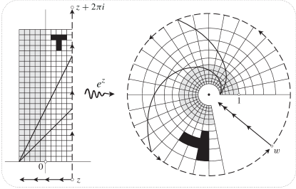
Figure 1. The action of the complex exponential map, as illustrated in Figure [10] on p. 82 of [24]. The pattern on the right is the image of the checkerboard pattern on the left. (Image courtesy of Tristan Needham.)

Recall that the complex exponential function is the holomorphic function $\exp\colon\mathbb{C}\to\mathbb{C}$ given by

(2.1) $$\exp(z)\mathrel{\vbox{\hbox{\scriptsize.}\hbox{\scriptsize.}}}=e^{z}=e^{x}\cdot e^{iy}=e^{x}\cdot(\cos(y)+i\sin(y)),\qquad\text{where }z=x+iy.$$

The representation (2.1) provides the following geometric interpretation of the action of the exponential map (see Figure 1), which the reader should keep in mind:

• The function $\exp$ maps horizontal lines to radial rays starting at the origin, and wraps vertical lines infinitely often around concentric circles centered at the origin. The modulus $|e^{z}|$ is large precisely when $\operatorname{Re}z$ is large and positive.

• In particular, the right half-plane $\mathbb{H}\mathrel{\vbox{\hbox{\scriptsize.}\hbox{\scriptsize.}}}=\{z\in\mathbb{C}\colon\operatorname{Re}z>0\}$ is mapped (in an infinite-to one manner) to the outside of the closed unit disc, and the left half-plane is mapped to the punctured unit disc.

• The exponential map is strongly expanding when $\operatorname{Re}z$ is large and positive, and strongly contracting when $\operatorname{Re}z$ is very negative.

Since the exponential map spreads the complex plane $\mathbb{C}$ over the punctured plane $\mathbb{C}^{*}$ in an infinite-to-one manner, it is not injective, and hence does not have a well-defined global inverse. Instead, we use branches of the logarithm: inverse functions to injective restrictions of $\exp$ (see [24, Section 2.VII]). It follows from (2.1) that such a branch exists wherever there is a continuous choice of the argument. For example, let $\vartheta\in\mathbb{R}$. Then

$$\exp\colon\{\zeta\in\mathbb{C}\colon\vartheta-\pi<\operatorname{Im}\zeta<\vartheta+\pi\}\to\{\omega\in\mathbb{C}\colon\operatorname{Arg}\omega\not\equiv-\vartheta\ (\operatorname{mod}\,2\pi)\}=\mathrel{\mathop{\mathchar 58\relax}}U$$

is bijective, and hence has a holomorphic inverse $L$ on $U$, given by

$$L(\omega)\mathrel{\vbox{\hbox{\scriptsize.}\hbox{\scriptsize.}}}=\log|\omega|+i\cdot\left(\vartheta+\operatorname{Arg}\frac{\omega}{e^{i\vartheta}}\right)\qquad(\omega\in U).$$

(Here, and throughout, $\log\colon(0,\infty)\to\mathbb{R}$ denotes the natural logarithm.) In particular, let $\Delta\subset\mathbb{C}$ be a disc that does not contain the origin, and let $\zeta_{0}\in\mathbb{C}$ with $e^{\zeta_{0}}\in\Delta$. Taking $\vartheta=\operatorname{Im}\zeta_{0}$, we see that there is a holomorphic map $L\colon\Delta\rightarrow\mathbb{C}$ with $L(e^{\zeta_{0}})=\zeta_{0}$ such that $e^{L(\omega)}=\omega$ and $\operatorname{Im}\zeta_{0}-\pi<\operatorname{Im}L(\omega)<\operatorname{Im}\zeta_{0}+\pi$ for all $\omega\in D$.

Note that we could replace $\Delta$ by any convex open set that omits the origin. More generally, branches of the logarithm exist on any simply-connected domain that does not contain the origin, but for us the above cases of discs and slit planes will be sufficient.

Devaney’s topological definition of chaos

We now introduce Devaney’s definition of chaos [10, §1.8] that was mentioned in the introduction. This is usually stated in the context of metric spaces (see below), but we shall restrict to the case of dynamical systems defined on subsets of the complex plane. Recall that, if $A\subset X\subset\mathbb{C}$, then $A$ is called dense in $X$ if every open set $U\subset\mathbb{C}$ that intersects $X$ also contains a point of $A$.

2.1 Definition (Devaney Chaos).

Let $X\subset\mathbb{C}$ be infinite, and let $f\colon X\to X$ be continuous. We say that $f$ is chaotic (in the sense of Devaney) if the following two conditions are satisfied.

1. The set of periodic points of $f$ is dense in $X$.

2. The function $f$ is topologically transitive; that is, for all open sets $U,V\subset\mathbb{C}$ that intersect $X$, there is a point $z\in U\cap X$ and $n\geq 0$ such that $f^{n}(z)\in V$.

Topological transitivity means precisely that we can move from any part of the space $X$ to any other by applying the function $f$ sufficiently often. This property clearly follows from the existence of a dense orbit (see Exercise 8.1). In particular, Theorem 1.2 is a consequence of Theorem 1.1. (However, in Section 5, we in fact argue in the converse direction – we first prove topological transitivity of the exponential map directly, and then deduce the existence of dense orbits.)

Sensitive dependence and spherical distances

Devaney’s original definition of chaos included a third condition: sensitive dependence on initial conditions. It is shown in [5] that this property is a consequence of topological transitivity and density of periodic points, which is why we were able to omit it in Definition 2.1.

It is nonetheless worthwhile to discuss sensitive dependence on initial conditions, since it encapsulates precisely the idea of “chaos” discussed in the introduction: Two points that are close together may end up a definitive distance apart after sufficiently many applications of the function $f$. (This phenomenon has become known in popular culture as the “butterfly effect”.) Moreover, in the case of the exponential map, we shall be able to establish sensitive dependence before proving either of the remaining two conditions.

To give the formal definition, we shall use the notion of a distance function (or metric) $d$ on a set $X$, as introduced e.g. in [9, Chapter 2] or [28, Chapter 2]. Readers unfamiliar with this definition need not despair: On the one hand, it is only used in this subsection; on the other, it will be sufficient to think of such a function informally as a formula that defines some notion of distance between two points of $X$. The simplest example of a distance function on $\mathbb{C}$ is the usual one, namely Euclidean distance $d(z,w)\mathrel{\mathop{\mathchar 58\relax}}=|z-w|$.

2.2 Definition (Sensitive dependence on initial conditions).

Let $X\subset\mathbb{C}$, let $f\mathrel{\mathop{\mathchar 58\relax}}X\to X$ be continuous, and let $d$ be a distance function on $X$. We say that $f$ exhibits sensitive dependence on initial conditions (with respect to $d$) if there exists a constant $\delta>0$ with the following property: For every non-empty open set $U\subset X$, there are points $x,y\in U$ and some $n\geq 0$ such that $d(f^{n}(x),f^{n}(y))\geq\delta$.

If we intend to use this definition, we ought to clarify which distance function we intend to use on the complex plane, and it is tempting to choose Euclidean distance.

This turns out to be a poor choice: even the “uninteresting” real exponential map discussed at the very beginning of this paper has sensitive dependence with respect to this distance (Exercise 8.2). The trouble is that, when orbits tend uniformly to infinity for a whole neighbourhood of our starting value, we would consider the corresponding behaviour to be “stable”, but orbits may end up extremely far apart in terms of Euclidean distance. This issue is resolved by instead using the so-called spherical distance, which is obtained by adjoining a single point at $\infty$ to the complex plane – so a point $z$ is close to $\infty$ whenever $|z|$ is large – and thinking of the resulting space $\mathbb{C}\cup\{\infty\}$ as forming a sphere in $3$-space. For this reason, the space $\mathbb{C}\cup\{\infty\}$ is called the Riemann sphere.

Instead of introducing spherical distance formally, let us use the informal picture above to decide what sensitive dependence with respect to the sphere should mean. If $\zeta,\omega\in\mathbb{C}$ are close to each other on the sphere, then there are only two possibilities: either both points are close to infinity, or they are also close in the Euclidean sense. Using this observation, we define sensitive dependence on the sphere directly and axiomatically:

2.3 Definition (Sensitive dependence with respect to spherical distance).

Let $f\colon\mathbb{C}\to\mathbb{C}$ be a continuous function. We say that $f$ has sensitive dependence with respect to spherical distance if there exist $\delta>0$ and $R>0$ with the following property. For every non-empty open set $U\subset\mathbb{C}$, there are $z,w\in U$ and $n\geq 0$ such that $|f^{n}(z)|\leq R$ and $|f^{n}(z)-f^{n}(w)|\geq\delta$.

It turns out (see Exercise 8.3) that Definition 2.3 implies sensitive dependence in the sense of Definition 2.2 – no matter which distance function we use on the complex plane.

3. A brief introduction to hyperbolic geometry

Hyperbolic geometry is a beautiful and powerful tool in one-dimensional complex analysis (as well as in higher-dimensional geometry). When discussing spherical distance in the previous section, we briefly encountered the idea of using a different notion of distance to the “standard” one; hyperbolic geometry is another example of this. If $U$ is any open subset of the complex plane that omits more than one point, then there is a natural notion of distance on $U$, called the hyperbolic metric. (For those who know differential geometry, this is the unique complete conformal metric of constant curvature $-1$ on $U$.) We only need a few elementary facts, all of which can be proved using elementary complex analysis. We shall first motivate these statements and then collect them in Theorem 3 and Proposition 4. For a more detailed introduction to the hyperbolic metric, we refer to the book [2] or the article [6].

Our starting point is the following classical consequence of the standard maximum modulus principle of complex analysis; see [17, Section 3.2] or [24, Section 7.VII].

3.1 Lemma (Schwarz lemma).

Suppose that $f\colon\mathbb{D}\rightarrow\mathbb{D}$ is holomorphic and $f(0)=0$. Then either

1. $|f(z)|<|z|$ for every non-zero $z$ in $\mathbb{D}$, and $|f^{\prime}(0)|<1$, or

2. there is a real constant $\vartheta$ such that $f(z)=e^{i\vartheta}z$ for all $z$, and $|f^{\prime}(0)|=|e^{i\vartheta}|=1$.

This lemma can be very useful, but its generality is limited because of the requirement that $f$ should fix $0$, and because its conclusion concerns only the derivative at the origin. However, we can move any point $a\in\mathbb{D}$ to zero using a Möbius transformation

(3.1) $$M\colon\mathbb{D}\to\mathbb{D};\qquad z\mapsto e^{i\vartheta}\frac{z-a}{1-\overline{a}z}$$

(where $\vartheta\in\mathbb{R}$ is arbitrary). So, if $f\colon\mathbb{D}\to\mathbb{D}$ is any holomorphic function, we can pre- and post-compose $f$ with suitable Möbius transformations and apply the Schwarz lemma. Using the chain rule to determine the derivative of the composition, we see that

(3.2) $$|f^{\prime}(z)|\cdot\frac{1-|z|^{2}}{1-|f(z)|^{2}}\leq 1\qquad\text{for all $z\in\mathbb{D}$.}$$

We can interpret (3.2) as saying that the derivative of $f$ is at most $1$ when calculated with respect to a different notion of distance (in the difference quotient usually used to define $|f^{\prime}|$). More precisely, we call the expression

(3.3) $$\frac{2|{\rm d}z|}{1-|z|^{2}}$$

the hyperbolic metric on $\mathbb{D}$. The idea is that if we have an “infinitesimal change” at the point $z$, then its corresponding size in the hyperbolic metric is obtained by multiplying its Euclidean length by the quantity

(3.4) $$\rho_{\mathbb{D}}(z)\mathrel{\vbox{\hbox{\scriptsize.}\hbox{\scriptsize.}}}=\frac{2}{1-|z|^{2}},$$

called the density of the hyperbolic metric. This can be made precise using the notions of differential geometry (formally, the metric is a way to measure the length of tangent vectors), but we can treat (3.3) simply as a formal expression.

3.1 Remark.

Although this expression is called a “metric”, it is not a “distance function” in the sense of the preceding section. However, it naturally gives rise to such a distance via the notion of arc-length; see [2, Chapter 3]. We note that the spherical metric can be similarly introduced via a conformal metric; that is, a metric that is a scalar multiple of the Euclidean metric at any point, where the scaling factor may depend on the point.

With our new notation, formula (3.2) states, in beautiful simplicity, that a holomorphic function $f\colon\mathbb{D}\to\mathbb{D}$ has hyperbolic derivative at most $1$ at every point, with equality if and only if $f$ is a Möbius transformation. What is even better is that we can transfer the metric to other domains.

2 Definition (Simply-connected domains).

An open connected set $U\subsetneq\mathbb{C}$ is called simply-connected if there is a conformal isomorphism (i.e., bijective holomorphic function) $\varphi\colon U\to\mathbb{D}$.

3.2 Remark.

Usually, $U$ is called simply-connected if $\mathbb{C}\setminus U$ has no bounded components; i.e., $U$ has no holes. The Riemann mapping theorem [1, Chapter 6] states that the two notions are equivalent. Our definition allows us to avoid using the Riemann mapping theorem, which is often not treated in a first course on complex analysis.

We can now state the following result, which collects the key properties of the hyperbolic metric. Its proof is elementary, using only the Schwarz lemma and the fact that the conformal automorphisms of $\mathbb{D}$ are precisely the Möbius transformations from (3.1); see Exercise 8.4. We leave it to the reader to fill in the details, or to consult [6, Theorem 6.4].

3 Theorem (Pick’s theorem).

For every simply-connected domain $U\subset\mathbb{C}$, there exists a unique conformal metric $\rho_{U}(z)|{\rm d}z|$ on $U$, called the hyperbolic metric, such that the following hold.

1. $\rho_{\mathbb{D}}(z)=\frac{2}{1-|z|^{2}}$ for all $z\in\mathbb{D}$;

2. if $f\colon U\to V$ is holomorphic, then $f$ does not increase the hyperbolic metric. I.e.,

   $$\|{\rm D}f(z)\|^{V}_{U}\mathrel{\vbox{\hbox{\scriptsize.}\hbox{\scriptsize.}}}=|f^{\prime}(z)|\cdot\frac{\rho_{V}(f(z))}{\rho_{U}(z)}\leq 1;$$

3. for any $z\in U$ and any $f$ as above, we have $\|{\rm D}f(z)\|^{V}_{U}=1$ if and only if $f$ is a conformal isomorphism between $U$ and $V$;

4. if $U\subsetneq V$, then $\rho_{U}(z)>\rho_{V}(z)$ for all $z\in U$.

(a) The unit disc $\mathbb{D}$

(b) The slit plane $\mathbb{C}\setminus(-\infty,0]$

(c) The right half-plane $\mathbb{H}$

(d) The strip $\{|\operatorname{Im}z|<\pi\}$

Figure 2. The hyperbolic metric in the unit disc and the simply-connected domains from Proposition 4. Red rings all have the same hyperbolic size; their Euclidean sizes shrink proportionally with the distance to the boundary. The images were kindly provided by Vladimir Bulatov (www.bulatov.org).

A key property of the hyperbolic metric on a simply-connected domain is that the density $\rho_{U}(z)$ is inversely proportional to the distance of $z$ to the boundary of $U$. In other words, suppose that a figure of constant hyperbolic size moves towards the boundary of $U$. Then its Euclidean size decreases proportionally with the distance to the boundary. (See Figure 2.) This is a general theorem – see [6, Formula (8.4)] – but in the domains that we shall be using, it can be checked explicitly from the following formulae.

4 Proposition (Examples of the hyperbolic metric).

1. For the right half plane $\mathbb{H}=\{z\in\mathbb{C}\colon\operatorname{Re}z>0\}$, $\displaystyle{\rho_{\mathbb{H}}(z)=\frac{1}{\operatorname{Re}z}}$.

2. For a strip of height $2\pi$: $\displaystyle{\rho_{\{z\in\mathbb{C}\colon|\operatorname{Im}z|<\pi\}}(z)=\frac{1}{2\cos(\operatorname{Im}(z)/2)}}$.

3. For the positively/negatively slit plane:

   $$\rho_{\mathbb{C}\setminus[0,\infty)}(z)=\frac{1}{2|z|\sin(\arg(z)/2)};\quad\rho_{\mathbb{C}\setminus(-\infty,0]}(z)=\frac{1}{2|z|\cos(\operatorname{Arg}(z)/2)}.$$

   (In the first case, the branch of the argument should be taken to range between $0$ and $2\pi$.)

3.3 Proof.

This can easily be verified by explicit computation using Theorem 3 (c), using the following conformal isomorphisms:

$$\varphi_{1}\colon\mathbb{H}\to\mathbb{D};\quad z\mapsto\frac{1-z}{1+z}; \varphi_{2}\colon S\to\mathbb{H};\quad z\mapsto e^{\frac{z}{2}};$$

$$\varphi_{3}\colon\mathbb{H}\to\mathbb{C}\setminus[0,\infty);\quad z\mapsto-z^{2}; \varphi_{4}\colon\mathbb{C}\setminus[0,\infty)\to\mathbb{C}\setminus(-\infty,0];\quad z\mapsto-z,$$

where $S=\{z\in\mathbb{C}\colon|\operatorname{Im}z|<\pi\}$. As an example, we consider the case of $\varphi_{2}$, and leave the remaining calculations to the reader. We have

$$\rho_{S}(z) =\rho_{\mathbb{H}}(\varphi_{2}(z))\cdot|\varphi_{2}^{\prime}(z)|=\frac{|\varphi_{2}(z)|}{2\operatorname{Re}\varphi_{2}(z)}=\frac{1}{2\cos(\arg(\varphi_{2}(z)))}=\frac{1}{2\cos(\operatorname{Im}(z)/2)}.$$

4. Escaping points and sensitive dependence

For the remainder of the article (unless stated otherwise), $f$ will always denote the exponential map

$$f\colon\mathbb{C}\to\mathbb{C};z\mapsto e^{z}.$$

We shall now prove the first part of Theorem 1.1, namely that the escaping set

$$I(f)\mathrel{\vbox{\hbox{\scriptsize.}\hbox{\scriptsize.}}}=\{z\in\mathbb{C}\colon f^{n}(z)\to\infty\}$$

is dense in the complex plane. The proof that we present here was briefly outlined in a paper of Mihaljević-Brandt and the second author [22, Remark on pp. 1583–1584].

1 Theorem (Density of the escaping set).

The set $I(f)$, consisting of those points $z_{0}$ whose $f$-orbits converge to infinity, is a dense subset of the complex plane $\mathbb{C}$.

The idea of the proof can be outlined as follows. Let $D\subset\mathbb{C}$ be any small round disc. Since $\mathbb{R}\subset I(f)$, and any preimage of an escaping point is also escaping, there is nothing to prove if $U$ contains a point $z$ whose orbit contains a point on the real axis.

Otherwise, $D$, $f(D)$ and all forward images $f^{n}(D)$ are contained in the slit plane

$$U\mathrel{\vbox{\hbox{\scriptsize.}\hbox{\scriptsize.}}}=\mathbb{C}\setminus[0,\infty).$$

Note that this set $U$ is backward invariant under $f$; i.e., $f^{-1}(U)\subseteq U$. It follows that every branch $L$ of the logarithm on $U$ is a holomorphic map $L\colon U\to U$, and hence locally contracts the hyperbolic metric of $U$, as discussed in the previous section.

Moreover, if $D\cap I(f)=\emptyset$, then the sequence of domains $f^{n}(D)$ necessarily has at least one finite accumulation point. Using the geometry of $U$, we shall see that this implies that the map $f$ expands the hyperbolic metric by a definite factor infinitely often along the orbit of $D$. On the other hand, the hyperbolic derivative of $f^{n}$ with respect to $U$ remains bounded as $n\to\infty$ by Pick’s theorem. This yields the desired contradiction.

From this summary of the proof, it is clear that understanding the expansion of the hyperbolic metric of $U$ by $f$ plays a key role in the argument. In the following lemma, we investigate where this expansion takes place.

2 Lemma (The exponential map expands the hyperbolic metric).

The complex exponential map $f$ locally expands the hyperbolic metric on the domain $U\mathrel{\vbox{\hbox{\scriptsize.}\hbox{\scriptsize.}}}=\mathbb{C}\setminus[0,\infty)$. That is, $\|{\rm D}f(\zeta)\|_{U}^{U}>1$ for all $\zeta\in f^{-1}(U)$.

Moreover, suppose that $\zeta_{n}\in f^{-1}(U)$ is a sequence with $\|{\rm D}f(\zeta_{n})\|_{U}^{U}\to 1$ as $n\to\infty$. Then $\min\bigl{(}|\zeta_{n}|,\operatorname{Arg}(\zeta_{n})\bigr{)}\to 0$ as $n\to\infty$.

4.1 Proof.

We shall give two justifications of this result. One is more conceptual and uses facts about the hyperbolic metric that were discussed, though not necessarily explicitly proved, in the previous section. The second is a completely elementary calculation; however, it hides some of the intuition.

To give the first argument, let $S$ be a connected component of the set

$$V\mathrel{\vbox{\hbox{\scriptsize.}\hbox{\scriptsize.}}}=f^{-1}(U)=\{a+ib\colon\frac{b}{2\pi}\notin\mathbb{Z}\}\subset U.$$

Then $S$ is a strip of height $2\pi$, and $f\colon S\to U$ is a conformal isomorphism. Let $\zeta\in S$ and set $\omega\mathrel{\vbox{\hbox{\scriptsize.}\hbox{\scriptsize.}}}=f(\zeta)\in U$. By Pick’s theorem, $f|_{S}$ is a hyperbolic isometry between $S$ and $U$, and hence

(4.1) $$\|{\rm D}f(\zeta)\|_{U}^{U}=\|{\rm D}f(\zeta)\|_{S}^{U}\cdot\frac{\rho_{S}(\zeta)}{\rho_{U}(\zeta)}=\frac{\rho_{S}(\zeta)}{\rho_{U}(\zeta)}>1.$$

Recall that the density at $z$ of the hyperbolic metric in a simply connected domain $G$ is comparable to $1/\operatorname{dist}(z,\partial G)$. (For $U$ and $S$, this can be verified explicitly, using Proposition 4.) We apply this fact twice: Notice first that every point in the strip $S$ has distance at most $\pi$ from the boundary, and hence $\rho_{S}$ is bounded from below by a positive constant. So if $\zeta_{n}$ is a sequence as in the claim, then, using the same fact for $\rho_{U}$, the distance $\operatorname{dist}(\zeta_{n},[0,\infty))=\operatorname{dist}(\zeta_{n},\partial U)\leq\operatorname{const}/\rho_{U}(\zeta_{n})$ remains bounded as $n\to\infty$. Also, by (4.1), $\zeta_{n}$ does not accumulate at any point of $U$. A sequence of points converging to $\infty$ while remaining within a bounded distance from the positive real axis must have arguments tending to $0$, and a point that is close to a finite point of $\partial U$ either has argument close to $0$ or is close to $0$ itself. So $\min\bigl{(}|\zeta_{n}|,\operatorname{Arg}(\zeta_{n})\bigr{)}\to 0$, as claimed.

On the other hand, the claims can be verified directly from the formulae. Indeed, let us write $\zeta=re^{i\vartheta}$ with $\vartheta\in(0,2\pi)$; then

$$\omega=f(\zeta)=e^{re^{i\vartheta}}=e^{r(\cos\vartheta+i\sin\vartheta)}.$$

Now we compute the hyperbolic derivative directly, using Proposition 4:

$$\|{\rm D}f(\zeta)\|_{U}^{U}=|f^{\prime}(\zeta)|\cdot\frac{2|\zeta|\cdot\sin(\frac{1}{2}\arg(\zeta))}{2|e^{\zeta}|\cdot\sin(\frac{1}{2}\arg(e^{\zeta}))}=\frac{r\cdot\sin(\vartheta/2)}{\sin(\frac{1}{2}\arg(e^{\zeta}))},$$

where $\arg(\zeta)$ and $\arg(e^{\zeta})$ are chosen in the range $(0,2\pi)$. To further simplify this expression, observe that $\arg(e^{\zeta})\equiv r\cdot\sin(\vartheta)\ (\operatorname{mod}\,2\pi)$. Since $|\sin|$ is $\pi$-periodic, we hence see that $|\sin(\arg(e^{\zeta})/2)|=\sin(r\sin(\vartheta)/2)$. Furthermore, $|\sin(x)|\leq|x|$ for all $x\in\mathbb{R}$, so

(4.2) $$\|{\rm D}f(\zeta)\|_{U}^{U} =\frac{r\cdot\sin(\vartheta/2)}{|\sin(\frac{r}{2}\cdot\sin\vartheta)|}\geq\frac{r\cdot\sin(\vartheta/2)}{\frac{r}{2}\cdot|\sin\vartheta|}$$

$$=\frac{2\cdot\sin(\vartheta/2)}{|\sin\vartheta|}=\frac{1}{|\cos(\vartheta/2)|}>1.$$

(In the final equality, we used the trigonometric formula $\sin(2x)=2\sin(x)\cos(x)$.) If $\zeta_{n}$ is such that $\|{\rm D}f(\zeta_{n})\|_{U}^{U}\to 1$, then (4.2) implies $|\cos(\vartheta_{n}/2)|\to 1$, where $\vartheta=\arg(\zeta_{n})$, and hence $\operatorname{Arg}(\zeta_{n})\to 0.$

4.2 Remark.

Observe that the second argument yields the stronger conclusion $\operatorname{Arg}(\zeta_{n})\to 0$. In fact, a slightly more careful look at the estimates shows that $\|{\rm D}f(\zeta_{n})\|_{U}^{U}\to 1$ if and only if $\operatorname{Arg}(\zeta_{n})\to 0$ and $\operatorname{Im}\zeta_{n}\to 0$ (see Exercise 8.5). However, this will not be required in the proofs that follow.

4.3 Proof (Proof of Theorem 1).

Let $w_{0}\in\mathbb{C}$ be arbitrary, and consider its orbit $(w_{n})_{n\geq 0}$, i.e. $w_{n}=f^{n}(w_{0})$. Let $D$ be a arbitrary disc around $w_{0}$; it is enough to show that $f^{n}(D)\cap I(f)\neq\emptyset$ for some $n$. So assume, by contradiction, that $f^{n}(D)\cap I(f)=\emptyset$ for all $n$. Since $[0,\infty)\subset I(f)$, we then have

$$D_{n}\mathrel{\vbox{\hbox{\scriptsize.}\hbox{\scriptsize.}}}=f^{n}(D)\subset U=\mathbb{C}\setminus[0,\infty)\qquad\text{for all $n\geq 0$.}$$

By Pick’s theorem 3, the hyperbolic derivative of $f^{n}$, as a map from $D$ to $U$, satisfies

$$\delta_{n}\mathrel{\vbox{\hbox{\scriptsize.}\hbox{\scriptsize.}}}=\|{\rm D}f^{n}(w_{0})\|_{D}^{U}=|(f^{n})^{\prime}(w_{0})|\cdot\frac{\rho_{U}(w_{n})}{\rho_{D}(w_{0})}\leq 1.$$

Set $\eta_{n}\mathrel{\vbox{\hbox{\scriptsize.}\hbox{\scriptsize.}}}=\|{\rm D}f(w_{n})\|_{U}^{U}$; then $\delta_{n+1}=\delta_{n}\cdot\eta_{n}$ for all $n\geq 0$.

By Lemma 2, we know that $\eta_{n}>1$. Hence, for the sequence $\delta_{n}$ to remain bounded, we must necessarily have $\eta_{n}\to 1$. Indeed, $(\delta_{n})_{n\geq 1}$ is an increasing and bounded, and hence convergent, sequence. Thus

$$\lim_{n\rightarrow\infty}\eta_{n}=\lim_{n\rightarrow\infty}\frac{\delta_{n+1}}{\delta_{n}}=\frac{\displaystyle{\lim_{n\rightarrow\infty}\delta_{n+1}}}{\displaystyle{\lim_{n\rightarrow\infty}\delta_{n}}}=1.$$

By Lemma 2, we see that

(4.3) $$\min\bigl{(}|w_{n}|,\operatorname{Arg}(w_{n})\bigr{)}\to 0,$$

and hence all finite accumulation points of $(w_{n})$ must lie in the interval $[0,\infty)$. Since $w_{0}$ is not in the escaping set, the set of such finite accumulation points is nonempty.

As this set is closed, we can let $z_{0}\in[0,\infty)$ be the smallest finite accumulation point of the sequence $(w_{n})$; say $w_{n_{k}}\to z_{0}$. Notice that $\operatorname{Re}w_{n_{k-1}}=\log|w_{n_{k}}|\rightarrow\log z_{0}<z_{0}$. By choice of $z_{0}$, the sequence $w_{n_{k-1}}$ cannot have a finite accumulation point, and hence $|\operatorname{Im}w_{n_{k-1}}|\to\infty$. This contradicts (4.3), and we are done.

The proof leaves open the possibility that the escaping set has nonempty interior (or even, a priori, that $I(f)=\mathbb{C}$). We shall now exclude this possibility, which then allows us to establish sensitive dependence on initial conditions.

3 Theorem (Preimages of the negative real axis).

Let $W\subset\mathbb{C}$ be open and nonempty. Then there are infinitely many numbers $n\geq 0$ such that $f^{n}(W)\cap(-\infty,0]\neq\emptyset$.

4.4 Remark.

This will also follow from the (stronger) results in the next section, but the proof we give here relies on the same ideas as that of Theorem 1, which gives the argument a nice symmetry.

4.5 Proof.

Let $D\subset W$ be an open disc. We shall first prove that there is at least one $n$ such that $f^{n}(D)$ intersects the negative real axis. So assume, by contradiction, that

$$f^{n}(D)\subset\tilde{U}\mathrel{\vbox{\hbox{\scriptsize.}\hbox{\scriptsize.}}}=\mathbb{C}\setminus(-\infty,0]$$

for all $n\geq 0$. By Theorem 1, there is a point $w_{0}\in D\cap I(f)$.

We proceed similarly as in the proof of Theorem 1, but now use the the hyperbolic metric of $\tilde{U}$. The set $\tilde{U}\mathrel{\vbox{\hbox{\scriptsize.}\hbox{\scriptsize.}}}=\mathbb{C}\setminus(-\infty,0]$ is not backward invariant, hence $f$ is not locally expanding at every point of $\tilde{U}$. However, there is expansion – even strong expansion – at points with sufficiently large real parts:

4 Claim.

If $\zeta\in f^{-1}(\tilde{U})$ and $\operatorname{Re}\zeta\geq 2$, then

$$\|{\rm D}f(\zeta)\|_{\tilde{U}}^{\tilde{U}}\geq\sqrt{2}.$$

4.6 Proof.

This follows by a similar calculation as in the proof of Lemma 2: if we write $\zeta=re^{i\vartheta}$ with $\vartheta\in(-\pi/2,\pi/2)$, then $f(\zeta)=e^{re^{i\vartheta}}=e^{r(\cos\vartheta+i\sin\vartheta)}$, and

$$\|{\rm D}f(\zeta)\|_{\tilde{U}}^{\tilde{U}} =|f^{\prime}(\zeta)|\cdot\frac{2|\zeta|\cdot|\cos\left(\frac{1}{2}\operatorname{Arg}(\zeta)\right)|}{2|e^{\zeta}|\cdot\bigl{|}\cos\bigl{(}\frac{1}{2}\operatorname{Arg}\bigl{(}e^{\zeta}\bigr{)}\bigr{)}\bigr{|}}$$

$$=\frac{r\cdot\cos(\vartheta/2)}{\bigl{|}\cos\bigl{(}\frac{1}{2}\operatorname{Arg}\bigl{(}e^{\zeta}\bigr{)}\bigr{)}\bigr{|}}\geq r\cdot\cos(\vartheta/2)\geq r\cdot\frac{\sqrt{2}}{2}\geq\sqrt{2}.$$

Now the proof proceeds along the same lines as before. Set $w_{n}\mathrel{\vbox{\hbox{\scriptsize.}\hbox{\scriptsize.}}}=f^{n}(w_{0})$ and $D_{n}\mathrel{\vbox{\hbox{\scriptsize.}\hbox{\scriptsize.}}}=f^{n}(D)$ for $n\geq 0$. Since $f^{n}\colon D\to\tilde{U}$ is a holomorphic map, we again have

$$\delta_{n}\mathrel{\vbox{\hbox{\scriptsize.}\hbox{\scriptsize.}}}=\|{\rm D}f^{n}(w_{0})\|^{\tilde{U}}_{D}\leq 1$$

for all $n$ by Pick’s Theorem. The numbers $\eta_{n}\mathrel{\vbox{\hbox{\scriptsize.}\hbox{\scriptsize.}}}=\|{\rm D}f(w_{n})\|_{\tilde{U}}^{\tilde{U}}=\frac{\delta_{n+1}}{\delta_{n}}$ need not be bounded below by $1$. However, since $w_{0}\in I(f)$, there is $n_{0}$ such that $\operatorname{Re}w_{n}\geq 2$ for $n\geq n_{0}$, and hence

$$\delta_{n}=\delta_{n_{0}}\cdot\|{\rm D}f^{n-n_{0}}(w_{n_{0}})\|_{\tilde{U}}^{\tilde{U}}\geq\delta_{n_{0}}\cdot 2^{(n-n_{0})/2}\to\infty.$$

This is a contradiction.

So $f^{n}(W)\cap(-\infty,0]\neq\emptyset$ for some $n$. To see that there are infinitely many such $n$, set $k_{0}=n$, and apply the result to $f^{k_{0}+1}(W)$ to find some $k_{1}>k_{0}$ with $f^{k_{1}}(W)\cap(-\infty,0]\neq\emptyset$. Proceeding inductively, we find an infinite sequence $(k_{j})$ with the desired property.

5 Corollary (Sensitive dependence).

The exponential map $f\colon\mathbb{C}\to\mathbb{C}$ has sensitive dependence on initial conditions with respect to spherical distance.

4.7 Proof.

We shall prove that $f$ satisfies Definition 2.3 with $R=1$ and $\delta=1$. Indeed, let $U\subset\mathbb{C}$ be open. Then, by Theorem 1, $U$ contains an escaping point $w$, and there is some $n_{0}$ such that $|f^{n}(w)|\geq 2$ for all $n\geq n_{0}$. By Theorem 3, there is $n_{1}>n_{0}$ and some point $z\in D$ such that $f^{n_{1}}(z)\in(-\infty,0]$. Hence, for $n\mathrel{\vbox{\hbox{\scriptsize.}\hbox{\scriptsize.}}}=n_{1}+1$, we have $|f^{n}(z)|\leq 1=R$ and $|f^{n}(w)-f^{n}(z)|\geq|f^{n}(w)|-|f^{n}(z)|\geq 1=\delta$, as desired.

5. Transitivity and dense orbits

Recall that topological transitivity, one of the properties required in the definition of chaos, means that we can move between any two nonempty open subsets of the complex plane by means of the iterates of $f$. The goal of this section is to establish transitivity, and deduce that there are also points with dense orbits.

1 Theorem (Topological transitivity).

If $U$, $V$ are nonempty and open, then there exists $n\geq 0$ such that $f^{n}(U)\bigcap V\neq\emptyset$.

We shall use the fact, established in the previous section, that the escaping set is dense in the plane. The key point is that $f$ is strongly expanding along the orbit of any escaping point $z_{0}$. Hence, for sufficiently large $n$, $f^{n}$ maps a small disc around $z_{0}$ to a set that contains a disc of radius $2\pi$ centred at $f^{n}(z_{0})$. By elementary mapping properties of the exponential map, the latter disc is spread, after two more applications of $f$, over a large part of the complex plane. This establishes topological transitivity.

We now provide the details of this argument. Let us begin with a simple observation.

2 Observation (Expansion along escaping orbits).

Let $z_{0}\in I(f)$, and set $z_{n}\mathrel{\vbox{\hbox{\scriptsize.}\hbox{\scriptsize.}}}=f^{n}(z_{0})$ for $n\geq 1$. Then $\operatorname{Re}z_{n}\to\infty$ and $|(f^{n})^{\prime}(z_{0})|\to\infty$ as $n\to\infty$.

5.1 Proof.

Since $z_{n+1}=e^{z_{n}}$ for all $n\geq 0$, we have

$$\operatorname{Re}z_{n}=\log|z_{n+1}|\to\infty$$

by definition of $I(f)$.

Furthermore, $|f^{\prime}(z_{n})|=|f(z_{n})|=|z_{n+1}|\to\infty$, and hence there is $N\in\mathbb{N}$ such that $|f^{\prime}(z_{n})|\geq 2$ for all $n\geq N$. For $m>N$, we can use the chain rule to compute the derivative of $f^{m}=f\circ f\circ\dots\circ f\circ f^{N}$:

$$|(f^{m})^{\prime}(z_{0})|=\bigl{|}\bigl{(}f^{N}\bigr{)}^{\prime}(z_{0})\bigr{|}\cdot\prod_{n=N}^{m-1}|f^{\prime}(z_{n})|\geq 2^{m-N}\cdot\bigl{|}\bigl{(}f^{N}\bigr{)}^{\prime}(z_{0})\bigr{|}\to\infty$$

as $m\to\infty$. Here we used the fact that $|(f^{N})^{\prime}(z_{0})|\neq 0$, since $f^{\prime}(z)\neq 0$ for all $z\in\mathbb{C}$.

We next prove the above-mentioned fact concerning the iterated images of small discs around escaping points.

3 Proposition (Small discs blow up).

Let $z_{0}\in I(f)$. For $n\geq 1$, set $z_{n}\mathrel{\vbox{\hbox{\scriptsize.}\hbox{\scriptsize.}}}=f^{n}(z_{0})$ and consider the disc $D_{n}$ of radius $2\pi$ centred at $z_{n}$; i.e. $D_{n}\mathrel{\vbox{\hbox{\scriptsize.}\hbox{\scriptsize.}}}=D_{2\pi}(z_{n})$. Then there are $n_{0}\in\mathbb{N}$ and a sequence $(\varphi_{n})_{n\geq n_{0}}$ of holomorphic maps $\varphi_{n}\colon D_{n}\rightarrow\mathbb{C}$ with the following properties:

1. $\varphi_{n}(z_{n})=z_{0}$,

2. $f^{n}(\varphi_{n}(z))=z$ for all $z\in D_{n}$,

3. $\sup_{z\in D_{n}}|\varphi^{\prime}_{n}(z)|\to 0$ as $n\to\infty$, and

4. $\operatorname{diam}(\varphi(D_{n}))\to 0$ as $n\to\infty$.

(That is, for large $n$ there is a branch $\varphi_{n}$ of $f^{-n}$ that takes $z_{n}$ back to $z_{0}$ and is uniformly strongly contracting.)

5.2 Proof.

Observe that c implies d. Indeed, for $z\in D_{n}$,

(5.1) $$|\varphi_{n}(z)-\varphi_{n}(z_{n})|\leq|z-z_{0}|\cdot\sup_{\zeta\in D_{n}}|\varphi_{n}^{\prime}(\zeta)|\leq 2\pi\sup_{\zeta\in D_{n}}|\varphi_{n}^{\prime}(\zeta)|$$

by the mean value inequality. Hence by c,

$$\operatorname{diam}(\varphi(D_{n}))\leq 4\pi\sup_{\zeta\in D_{n}}|\varphi_{n}^{\prime}(\zeta)|\to 0\qquad\text{as $n\to\infty$.}$$

To prove the proposition, first assume additionally that $|z_{n}|\geq 2\pi+2$ for all $n\geq 1$. In this case, none of the discs $D_{n}$ contain the origin. For each $n\geq 1$, let $L_{n}\colon D_{n}\rightarrow\mathbb{C}$ be the branch of the logarithm with $L_{n}(z_{n})=L_{n}(e^{z_{n-1}})=z_{n-1}$. What can we say about the range of this map $L_{n}$? Since $|z_{n}|\geq 2\pi+2$ for all $n\geq 1$, we have $|z|\geq 2$ for all $z\in D_{n}$, and hence

$$|L_{n}^{\prime}(z)|=1/|z|\leq 1/2.$$

Again using the mean value inequality, we see that

(5.2) $$|L_{n}(z)-z_{n-1}|=|L_{n}(z)-L(z_{n})|\leq\sup_{\zeta\in D_{n}}|L^{\prime}(\zeta)|\cdot\pi$$

for each $n$ and all $z\in D_{n}$. In particular, and importantly, $L_{n}(D_{n})\subset D_{n-1}$.

It follows by induction that the composition $\varphi_{n}\mathrel{\vbox{\hbox{\scriptsize.}\hbox{\scriptsize.}}}=L_{1}\circ L_{2}\circ\dots\circ L_{n}$ is defined on $D_{n}$, with $|\varphi_{n}^{\prime}(z)|\leq 2^{-n}$ for $z\in D_{n}$. Hence $\varphi_{n}$ satisfies c, and a and b hold by construction. This completes the proof when $|z_{n}|\geq 2\pi+2$ for all $n\geq 1$.

If this is not the case, then – since $z_{0}$ is an escaping point – there still exists $n_{1}$ such that $|z_{n}|\geq 2\pi+2$ for all $n>n_{1}$. We can thus apply the preceding case to the point $z_{N}$. This means that, for every $n>n_{1}$, there is a holomorphic map $\psi_{n}\colon D_{n}\to D_{n_{1}}$ such that

1. $\psi_{n}(z_{n})=z_{m}$,

2. $f^{n-n_{1}}(\psi_{n}(z))=z$ for all $z\in D_{n}$,

3. $\sup_{z\in D_{n}}|(\psi_{n})^{\prime}(z)|\to 0$ as $n\to\infty$, and

4. $\operatorname{diam}(\psi_{n}(D_{n}))\to 0$ as $n\to\infty$.

By the inverse function theorem, there exists a neighbourhood $U$ of $z_{n_{1}}$ and a branch $\pi\colon U\to\mathbb{C}$ of $f^{-n_{1}}$ mapping $z_{n_{1}}$ to $z_{0}$. (This also follows from repeated applications of suitable branches of the logarithm. Observe that $z_{n}=f(z_{n-1})\neq 0$ for $n\geq 1$.)

Now let $K$ be a small closed disc around $z_{n_{1}}$ with $K\subset U$. By d, we have $\psi_{n}(D_{n})\subset K$ for sufficiently large $n$ – say, for $n\geq n_{0}$. Hence we can define

$$\varphi_{n}\colon D_{n}\to\mathbb{C};\quad\varphi_{n}(z)\mathrel{\vbox{\hbox{\scriptsize.}\hbox{\scriptsize.}}}=\pi(\psi_{n}(z)).$$

This map satisfies a and b by definition, and

$$\sup_{z\in D_{n}}|\varphi_{n}^{\prime}(z)|=\sup_{z\in D_{n}}\bigl{(}|\psi_{n}^{\prime}(z)|\cdot|\pi^{\prime}(\psi_{n}(z))|\bigr{)}\leq\max_{z\in D_{n}}|\psi_{n}^{\prime}(z)|\cdot\sup_{w\in K}|\pi^{\prime}(w)|\to 0$$

by property c) of $\psi_{n}$. (Since $K$ is compact, the continuous function $|\pi^{\prime}|$ assumes its maximum on $K$, which is independent of $n$.)

As mentioned above, after two additional iterates the discs in the preceding Proposition will cover a large portion of the plane, as long they lie far enough to the right:

4 Observation (Images of large discs).

Let $K$ be any nonempty compact subset of the punctured plane $\mathbb{C}\setminus\{0\}$. Then there is $\rho>0$ with the following property. Suppose that $D$ is a disc of radius $2\pi$, centred at a point having real part at least $\rho$. Then $K\subset f^{2}(D)$.

5.3 Proof.

The disc $D$ contains a closed square of side-length $2\pi$, also centred at $\zeta$. Let $a=\operatorname{Re}\zeta-\pi$ be the real part of the left vertical edge of $S$, then $a+2\pi=\operatorname{Re}\zeta+\pi$ is the real part of the right vertical edge of $S$. What is the image of $S$ under $f$? Looking back at Figure 1, we see that it is precisely a closed round annulus $A$ around the origin, with inner radius $r_{-}=e^{a}$ and outer radius $r_{+}=e^{a+2\pi}$.

Figure 3. In the proof of Observation 4, the square $S$ is mapped to a large annulus $A$. The rectangle $R$ shown in $A$ maps to an annulus of huge outer radius and tiny inner radius, containing the compact set $K$.

If $a$ is sufficiently large, then $A$ is a rather thick annulus with large inner radius. It follows that $A$ contains a long rectangular strip of height $2\pi$, and the image of this strip will cover most of the complex plane, including the compact set $K$. More precisely, suppose that $a\geq 0$; then $r_{+}-r_{-}\geq e^{2\pi}>2\pi$. Hence we can fit a maximal rectangle $R$ of height $2\pi$ into $A$, symmetrically with respect to the imaginary axis and tangential to the inner boundary circle of $A$. (See Figure 3.)

Let $\ell$ be the maximal real part of $R$ (i.e., $\ell$ is half the horizontal side-length of $R$). We can compute $\ell$ using the Pythagorean Theorem:

$$\ell^{2}=r_{+}^{2}-(r_{-}+2\pi)^{2}>r_{+}^{2}-4r_{-}^{2}=(e^{4\pi}-4)\cdot e^{2a}>e^{2a},$$

provided that $r_{-}\geq 2\pi$. Hence we see that $\ell>e^{a}$, and the image of $R$ includes all points of modulus between $e^{-\ell}$ and $e^{\ell}$.

In particular, we can set

$$\rho\mathrel{\vbox{\hbox{\scriptsize.}\hbox{\scriptsize.}}}=3\pi+\max_{z\in K}\bigl{|}\log|z|\bigr{|}.$$

If $\operatorname{Re}\zeta\geq\rho$, then we have $a\geq 2\pi$, and $\ell>e^{a}>a>\bigl{|}\log|z|\bigr{|}$. The claim follows.

As a consequence, we obtain the following stronger version of Theorem 1.

5 Corollary (Open sets spread everywhere).

Let $K\subset\mathbb{C}\setminus\{0\}$ be compact, and let $U\subset\mathbb{C}$ be open and nonempty. Then there is some $N\in\mathbb{N}$ such that $K\subset f^{n}(U)$ for all $n\geq N$.

5.4 Remark.

To deduce the original statement of Theorem 1, simply choose $K$ to consist of a single point in $V$.

5.5 Proof.

Since the escaping set is dense in the plane, there exists some $z_{0}\in I(f)\cap U$. Set $z_{n}\mathrel{\vbox{\hbox{\scriptsize.}\hbox{\scriptsize.}}}=f^{n}(z_{0})$ for $n\geq 1$, and let $D_{n}\mathrel{\vbox{\hbox{\scriptsize.}\hbox{\scriptsize.}}}=D_{2\pi}(z_{n})$, $n_{0}$ and $\varphi_{n}$ be as in Proposition 3. Also let $\rho$ be the number from Observation 4 (for the same set $K$). Since $z_{0}$ is an escaping point, and by part (d) of Proposition 3, we can choose $N_{1}\geq n_{0}$ such that $\operatorname{Re}z_{n}\geq\rho$ and $\varphi_{n}(D_{n})\subset U$ for all $n\geq N_{1}$.

Let $n\geq N_{1}$. Then

$$f^{n+2}(U)\supset f^{n+2}(\varphi_{n}(D_{n}))=f^{2}(f^{n}(\varphi_{n}(D_{n})))=f^{2}(D_{n})\supset K$$

by Observation 4. Hence the claim holds with $N\mathrel{\vbox{\hbox{\scriptsize.}\hbox{\scriptsize.}}}=N_{1}+2$.

The existence of dense orbits is closely related, and often equivalent, to that of topological transitivity. Indeed, we can deduce the former from Theorem 1, by using the Baire category theorem [28, Exercise 16 in Chapter 2]. This theorem implies that any countable intersections of open and dense subsets of the complex plane is itself dense and uncountable.

6 Corollary (Dense orbits).

The set $\mathcal{T}$ of all points $z_{0}\in\mathbb{C}$ with dense orbits under the exponential map is uncountable and dense in $\mathbb{C}$.

5.6 Proof.

Let $D\subset\mathbb{C}$ be any non-empty open set. By Theorem 1, the inverse orbit

$$\mathcal{O}^{-}(D)\mathrel{\vbox{\hbox{\scriptsize.}\hbox{\scriptsize.}}}=\bigcup_{n\geq 0}f^{-n}(D)$$

is a dense subset of $\mathbb{C}$. Note that $\mathcal{O}^{-}(D)$ is also open, as a union of open subsets.

Now consider the countable collection

$$\mathcal{D}\mathrel{\vbox{\hbox{\scriptsize.}\hbox{\scriptsize.}}}=\{D_{r}(z)\colon\operatorname{Re}z,\operatorname{Im}z,r\in\mathbb{Q}\}$$

of open discs with rational centres and radii. Clearly $z_{0}\in\mathcal{T}$ if and only if the orbit of $z_{0}$ enters every element of $\mathcal{D}$ at least once, i.e.

$$\mathcal{T}=\bigcap_{D\in\mathcal{D}}\mathcal{O}^{-}(D).$$

Hence $\mathcal{T}$ is indeed uncountable and dense, as a countable intersection of open and dense subsets of $\mathbb{C}$.

6. Density of periodic points

We are now ready to complete the proof that the exponential map is chaotic, by proving density of the set of periodic points. In fact, we shall prove slightly more, namely that repelling periodic points of $f$ are dense in the plane. Here a periodic point $p$, with $f^{n}(p)=p$, is called repelling if $|(f^{n})^{\prime}(p)|>1$. This ensures that any point $z\neq p$ close to $p$ is (initially) “repelled” away from the orbit of $p$ – density of such points gives another indication that the dynamics of the exponential map is highly unstable! (It is, however, not difficult to show directly that all periodic points of $f$ are repelling; see Exercise 8.8.)

1 Theorem (Density of repelling periodic points).

Let $U\subset\mathbb{C}$ be open and nonempty. Then there exists a repelling periodic point $p\in U$.

The idea of the proof is, again, to begin with an escaping point $z_{0}$. Our goal is to find an inverse branch of an iterate of $f$ that maps a neighbourhood of $z_{0}$ back into itself, with strong contraction. Then the existence of a periodic point follows from the contraction mapping theorem [9, Theorem 3.6] (also known as the Banach fixed point theorem). We noticed already in the last section that the disc $D_{n}$ of radius $2\pi$ around the $n$-th orbit point $z_{n}$ can be pulled back along the orbit in one-to-one fashion (Proposition 3). We need to be able to “close the loop”, by pulling back a small disc around $z_{0}$ into $D_{n}$. In other words, we are looking for a more precise version of Observation 4, as follows.

2 Lemma (Inverse branches of $f^{2}$).

Let $z_{0}\in\mathbb{C}\setminus\{0\}$. Then there are a disc $\Delta$ centered at $z_{0}$ and a number $\rho\geq 0$ with the following property:

For any disc $D$ of radius $2\pi$ centred at a point with real part at least $\rho$, there is $\varphi\colon\Delta\rightarrow D$ such that $f^{2}(\varphi(z))=z$ and $|\varphi^{\prime}(z)|\leq 1$ for all $z\in\Delta$.

6.1 Remark.

In other words, there exists a disc $\Delta$ around $z_{0}$ that is not only covered by $f^{2}(D)$ (as we know it must be from Observation 4), but on which we can even define a branch of $f^{-2}$ that takes it back into $D$. It is not difficult to extend the result, with a similar proof, to see that this is true for any disc $\Delta$ – and indeed any simply-connected domain – whose closure is bounded away from $0$ and $\infty$.

6.2 Proof.

Set $\varepsilon\mathrel{\vbox{\hbox{\scriptsize.}\hbox{\scriptsize.}}}=\frac{|z_{0}|}{2}$ and $\Delta\mathrel{\vbox{\hbox{\scriptsize.}\hbox{\scriptsize.}}}=D_{\varepsilon}(z_{0})$. For any $n\in\mathbb{Z}$, there is a branch $L_{n}$ of the logarithm on $\Delta$ whose values have imaginary parts between $\operatorname{Arg}z_{0}+(2n-1)\pi$ and $\operatorname{Arg}z_{0}+(2n+1)\pi)$. Each $L_{n}$ is continuous on $\Delta$ and satisfies $f(L_{n}(z))=z$ for all $z\in\Delta$.

Consider the sets $V_{n}\mathrel{\vbox{\hbox{\scriptsize.}\hbox{\scriptsize.}}}=L_{n}(\Delta)$, with $n\in\mathbb{Z}$; then $V_{n}=V_{0}+2\pi in$. So the $V_{n}$ form a linear sequence of domains of uniformly bounded diameter, tending to infinity in the direction of the positive and negative imaginary axes. Consider all preimage components of some $V_{n}$ under $f$, for $n\neq 0$ (since $V_{0}$ might contain the origin). On each of these, we can define a branch of $f^{-2}$ taking values in $\Delta$ – hence we should show that any disc $D$ of radius $2\pi$ contains at least one such component, provided that its centre lies sufficiently far to the right. This should be clear from the mapping behaviour of the exponential map (Figure 1). Indeed, for every odd multiple of $\pi/2$, there is a sequence of sets in question whose imaginary parts tend to this value, and having real parts closer and closer together (see Figure 4).

Figure 4. This is an illustration of the proof of Lemma 2. Shown are the first and second preimage component of the disc $\Delta=D_{\frac{3}{2}}(3)$.

More formally, consider the points $w_{n}\mathrel{\vbox{\hbox{\scriptsize.}\hbox{\scriptsize.}}}=L_{n}(z_{0})\in V_{n}$. Set $\rho_{1}\mathrel{\vbox{\hbox{\scriptsize.}\hbox{\scriptsize.}}}=|w_{0}|+3$ and let $D$ be a disc of radius $2\pi$ centred at a point $\zeta$ with $\operatorname{Re}\zeta\geq\rho_{1}$. Since $w_{n}=w_{0}+2\pi in$, we can find $n_{0}\geq 1$ such that

(6.1) $$|e^{\zeta}|-\pi\leq|w_{n_{0}}|\leq|e^{\zeta}|+\pi.$$

Furthermore, choose $m$ such that $|\operatorname{Im}\zeta-(4m+1)\pi/2|\leq\pi$, and let $\psi$ be the branch of the logarithm mapping the upper half-plane to the strip $\{z\in\mathbb{C}\colon 2m\pi<\operatorname{Im}z<(2m+1)\pi\}$.

Let $w\in V_{n_{0}}$. Then $|\operatorname{Im}\psi(w)-\operatorname{Im}\zeta|\leq 3\pi/2$ by choice of $\psi$. Furthermore, by definition of $\Delta$ and $L_{n}$, we have

$$|\operatorname{Re}w-\operatorname{Re}w_{n_{0}}|=\left|\log\frac{|w|}{|w_{n_{0}}|}\right|\leq\log 2.$$

By (6.1), we conclude that

$$|e^{\zeta}|-2\pi-\log 2\leq|w|\leq|e^{\zeta}|+2\pi+\log 2.$$

Dividing by $|e^{\zeta}|$, and recalling that $\operatorname{Re}\zeta\geq\rho_{1}>3>\log 5\pi$, we see that

$$\frac{1}{2}<1-\frac{2\pi+\log 2}{|e^{\zeta}|}<\frac{|w|}{|e^{\zeta|}}<1+\frac{2\pi+\log 2}{|e^{\zeta}|}<2.$$

Hence

$$|\operatorname{Re}\psi(w)-\operatorname{Re}\zeta|=|\log|w|-\operatorname{Re}\zeta|=\left|\log\frac{|w|}{|e^{\zeta}|}\right|<\log 2.$$

Thus

$$|w-\zeta|<3\pi/2+\log 2<2\pi,$$

and hence $\psi(V_{n})\subset D$. Hence the branch $\varphi\mathrel{\vbox{\hbox{\scriptsize.}\hbox{\scriptsize.}}}=\psi\circ\varphi_{n}$ indeed maps $\Delta$ into $D$. Moreover,

$$\varphi_{n}^{\prime}(z)=\frac{1}{|z|}\leq\frac{2}{|z_{0}|}$$

for all $z\in\Delta$, while

$$|\psi^{\prime}(z)|=\frac{1}{|z|}\leq\frac{2}{e^{\zeta}}$$

on $V_{n}$. Hence, if we choose $\rho\mathrel{\vbox{\hbox{\scriptsize.}\hbox{\scriptsize.}}}=\max(\rho_{1},\log 4-\log|z_{0}|)$, then $|\varphi^{\prime}(z)|\leq 1$ for all $z\in\Delta$, as required.

6.3 Proof (Proof of Theorem 1).

Let $U\subset\mathbb{C}$ be open and nonempty. By Theorem 1, there is an escaping point $z_{0}\in U\setminus\{0\}$. Choose a disc $\Delta$ around $z_{0}$ and $\rho>0$ and as in Lemma 2. By shrinking $\Delta$, if necessary, we may suppose that $\Delta\subset U$.

Let $\Delta_{1}$ be a smaller disc also centred at $z_{0}$. so that $\overline{\Delta_{1}}\subset\Delta$. As in Section 5, set $z_{n}\mathrel{\vbox{\hbox{\scriptsize.}\hbox{\scriptsize.}}}=f^{n}(z_{0})$ and $D_{n}\mathrel{\vbox{\hbox{\scriptsize.}\hbox{\scriptsize.}}}=D_{2\pi}(z_{n})$. Let $(\varphi_{n})_{n\geq n_{0}}$ be the inverse branches from Proposition 3. By conclusions d and c of that Proposition, we may assume that $n_{0}$ is large enough to ensure that $\varphi_{n}(z)\in\Delta_{1}$ and $|\varphi_{n}^{\prime}(z)|\leq 1/2$ for all $z\in D_{n}$.

Since $z_{0}$ is an escaping point, there is $N\geq n_{0}$ such that $\operatorname{Re}z_{n}\geq\rho$ for all $n\geq N$. By Lemma 2, there is thus a branch $\psi_{n}$ of $f^{-2}$ that maps $\Delta$ into $D_{n}$, with $|\psi_{n}^{\prime}(z)|\leq 1$ for all $z\in\Delta$.

It follows that $\varphi_{n}(\psi_{n}(\overline{\Delta_{1}}))\subset\varphi_{n}(D_{n})\subset\Delta_{1}$, and that $\varphi_{n}\circ\psi_{n}\colon\overline{\Delta_{1}}\to\overline{\Delta_{1}}$ is a contraction map. As $\overline{\Delta_{1}}$ is compact, and hence complete, this function has a fixed point $p\in\overline{\Delta}$ by the contraction mapping theorem. By construction,

$$f^{n+2}(p) =f^{2}(f^{n}(\varphi_{n}(\psi_{n}(p))))=f^{2}(\psi_{n}(p))=p\qquad\text{and}$$

$$|(f^{n+2})^{\prime}(p)| =\frac{1}{|\psi_{n}^{\prime}(p)|\cdot|\varphi_{n}^{\prime}(\psi_{n}(p))|}\geq 2.$$

Hence $p$ is indeed a repelling periodic point of $f$, as required.

7. Further results and open problems

The realization that the exponential map $f$ acts chaotically on the complex plane is not the end of the story. Rather, it leads to further questions about the qualitative behaviour of $f$, and much research has been done since Misiurewicz’s work. The picture is still far from complete, and several interesting questions remain open. Here, we restrict to a small selection of results and ideas, referring to the literature for further information.

The escaping set of the exponential. The escaping set $I(f)$ of the exponential map played an important role in our proof of Theorems 1.1 and 1.2. We saw in Theorem 1 that this set is dense in the plane, and hence it is plausible that a thorough study of its fine structure will yield information also about the non-escaping part of the dynamics. We already saw that $I(f)$ contains the real axis together with all of its preimages under iterates of $f$– but there are many other escaping points! Indeed, Devaney and Krych [13] observed the existence of uncountably many different curves to infinity in $I(f)$, most of which do not reach the real axis under iteration. Later, Schleicher and Zimmer [29] were able to show that every point of $I(f)$ can be connected to infinity by a curve in $I(f)$.

Maximal curves in the escaping set are referred to as “rays” or “hairs”, and they provide a structure that can be exploited in the study of the wider dynamics of $f$. However, the way in which these rays fit together to form the entire escaping set is rather non-trivial. For example, while each path-connected component of $I(f)$ is such a curve, and is relatively closed in $I(f)$ (i.e., rays do not accumulate on points that belong to other rays) the escaping set nonetheless turns out to be a connected subset of the plane [27]. Furthermore, while many rays end at a unique point in the complex plane, some have been shown to accumulate everywhere upon themselves [12, 26], resulting in a very complicated topological picture. For which rays this can occur, and whether other types of accumulation behaviour are possible, requires further research.

Taken together, these results provide some indication that the escaping set is a rather complicated object. In fact, even iterated preimages of the negative real axis (all of which are simple curves tending to infinity in both directions) result in highly nontrivial phenomena and open questions. In 1993, Devaney [11] showed that the closure of a certain natural sequence of such preimages has some “pathological” topological properties. He also formulated a conjecture concerning the structure of this set and its stability under certain perturbations of the map $f$, which remains open to this day.

Measurable dynamics of the exponential. Corollary 6 (and its proof) means that, topologically, “most” points have a dense orbit. It is natural to ask also about the behaviour of “most” points with respect to area: If we pick a point $z\in\mathbb{C}$ at random will its orbit be dense? Lyubich [20] and Rees [25] independently gave an answer in the 1980s: For a random point $z\in\mathbb{C}$, the orbit of $z$ is not dense; rather, its set of limit points coincides precisely with the orbit of $0$. In other words, after a certain number of steps, the orbit will come very close to $0$, and then follow the orbit $\{0,1,e,e^{e},\dots\}$ for a finite number of steps. Our point might then spend some additional time close to $\infty$, until it maps into the left half-plane. In the next step, it ends up even closer to $0$, and so on. We can furthermore also ask about the relative “sizes” of the sets of points with various other types of behaviour (for example, with respect to fractal dimension). It again turns out that there is a rich structure from this point of view; see e.g. [21, 30, 19].

Transcendental dynamics. To place the material in this paper in its proper context, let us finally discuss iterating a holomorphic self-map $f\colon\mathbb{C}\to\mathbb{C}$ of the complex plane in general. To obtain interesting behaviour, we assume that $f$ is non-constant and non-linear. As before, a key question is how the behaviour of orbits varies under perturbations of the starting point $z_{0}$. To this end, one divides the starting values into two sets: The closed set of points near which there is sensitive dependence on initial conditions is called the Julia set $J(f)$, while its complement – where the behaviour is stable – is the Fatou set $F(f)=\mathbb{C}\setminus J(f)$. (See [7] for formal definitions and further background.) By the magic of complex analysis, the – rather mild – notion of instability used to define the Julia set always leads to globally chaotic dynamics:

1 Theorem (Chaos on the Julia set).

The Julia set $J(f)$ is always uncountably infinite, and $f^{-1}(J(f))=J(f)$. Furthermore, the function $f\colon J(f)\to J(f)$ is chaotic in the sense of Devaney.

The key part of this theorem is the density of periodic points in the Julia set. That $J(f)$ is uncountable and that $f$ is topologically transitive was known already (albeit in different terminology) to Pierre Fatou and (in the case of polynomials) Gaston Julia, who independently founded the area of holomorphic dynamics in the early twentieth century. For polynomials – and indeed for rational functions – the density of periodic points in the Julia set was also established by Fatou and Julia, but it took about half a century until Baker [3] completed the proof for general entire functions.

With this general terminology, Misiurewicz’s theorem says precisely that $F(\exp)=\emptyset$. (We emphasize that there are many entire functions with nonempty Fatou set. As an example, consider $f(z)\mathrel{\vbox{\hbox{\scriptsize.}\hbox{\scriptsize.}}}=(e^{z}-1)/4$. Then $f^{n}(z)\to 0$ for $|z|<1$, and hence the entire unit disc is in the Fatou set.) It can be shown that there are only a few possible types of behaviour for points in the Fatou set of an entire function [7, § 4.2]. Using classical methods, most of these can be excluded fairly easily in the case of the exponential map; the difficult part is to show that there can be no wandering domain, i.e. a connected component $U$ of the Fatou set such that $f^{n}(U)\cap U=\emptyset$ for all $n>0$. Misiurewicz used the specific properties of the exponential function, but more general tools for ruling out the existence of wandering domains have since been developed. The most famous is due to Sullivan, who showed that rational functions never have wandering domains, answering a question left open by Fatou. Sullivan’s argument, which uses deep results from complex analysis, can be extended to classes of entire functions containing the exponential map [4, 15, 18]. As mentioned in the introduction, this provides an alternative (though highly non-elementary) method of establishing Misiurewicz’s theorem. The study of wandering domains, and when they can occur, continues to be an active topic of research in transcendental dynamics; we refer to [22] for a discussion and references.

8. Exercises

8.1 Exercise (Topological transitivity and dense orbits).

Let $X\subset\mathbb{C}$, and let $f\colon X\to X$ be a continuous function. We say that $x_{0}\in X$ has a dense orbit if the set of accumulation points of the orbit of $x_{0}$ is dense in $X$. (Note that this differs subtly from the requirement that the orbit of $x_{0}$ is dense when thought of as a subset of $X$. However, the two conditions are equivalent if $X$ has no isolated points.)

Prove: if there is a point with a dense orbit under $f$, then $f$ is topologically transitive.

8.2 Exercise (Problems with using Euclidean distance in sensitive dependence).

Show that the real exponential map $f\colon\mathbb{R}\to\mathbb{R};x\mapsto e^{x}$, exhibits sensitive dependence on initial conditions with respect to Euclidean distance $d(x,y)=|x-y|$.

8.3 Exercise (Sensitive dependence for distance functions).

Let $f\colon\mathbb{C}\to\mathbb{C}$ be continuous and have sensitive dependence with respect to spherical distance.

Prove: If $d\colon\mathbb{C}\times\mathbb{C}\to[0,\infty)$ is any distance function that is topologically equivalent to Euclidean distance (i.e., a round open disc around a point $z_{0}$ contains some disc around $z_{0}$ in the sense of the distance $d$, and vice versa), then $f$ has sensitive dependence with respect to $d$. (So sensitive dependence with respect to spherical distance is the strongest such condition we can impose.)

Hint. Observe that the possible pairs $(f^{n}(z),f^{n}(w))$ in Definition 2.3 all belong to a closed and bounded subset of $\mathbb{C}^{2}$, which depends only on $\delta$ and $R$. Then use the fact that $d$ is continuous as a function of two complex variables (with respect to Euclidean distance).

8.4 Exercise (Automorphisms of the disc).

Suppose that $f\colon\mathbb{D}\to\mathbb{D}$ is a conformal automorphism (i.e. holomorphic and bijective) with $f(0)=0$. Conclude, using the Schwarz lemma, that $f$ is a rotation around the origin. Deduce that any conformal automorphism $f\colon\mathbb{D}\to\mathbb{D}$ is of the form (3.1).

8.5 Exercise (Expansion of the exponential map).

Strengthen Lemma 2 by showing that $\|{\rm D}f(\zeta_{n})\|_{U}^{U}\to 1$ if and only if $\operatorname{Arg}(\zeta_{n})\to 0$ and $\operatorname{Im}\zeta_{n}\to 0$. (Hint. Use the fact that $|\sin(x)|/|x|\to 1$ if and only if $|x|\to 0$.)

8.6 Exercise (Strong hyperbolic expansion for large real parts).

For the domain $\tilde{U}$ in the proof of Theorem 3, show that even $\|{\rm D}f(\zeta)\|_{\tilde{U}}^{\tilde{U}}\to\infty$ as $\operatorname{Re}\zeta\to\infty$.

(Either use a direct calculation as in the proof of the Claim, or a more conceptual explanation as in the first part of the proof of Lemma 2.)

8.7 Exercise (Extremely sensitive dependence).

Strengthen Corollary 5 by showing that the exponential map satisfies Definition 2.3 for any choice of $R,\delta>0$.

8.8 Exercise (No nonrepelling orbits).

Use Lemma 2 to show that all periodic points of the exponential map are repelling.

(Hint. Observe that, at a periodic point of period $n$, the hyperbolic derivative of $f^{n}$ agrees precisely with the usual (Euclidean) derivative.)

References

- [1] L. V. Ahlfors, Complex analysis, third ed., McGraw-Hill Book Co., New York, 1978, International Series in Pure and Applied Mathematics.
- [2] J. W. Anderson, Hyperbolic geometry, second ed., Springer Undergraduate Mathematics Series, Springer-Verlag London, Ltd., London, 2005.
- [3] I. N. Baker, Repulsive fixpoints of entire functions, Math. Z. 104 (1968), 252–256.
- [4] I. N. Baker and P. J. Rippon, Iteration of exponential functions, Ann. Acad. Sci. Fenn. Ser. A I Math. 9 (1984), 49–77.
- [5] J. Banks, J. Brooks, G. Cairns, G. Davis, and P. Stacey, On Devaney’s definition of chaos, Amer. Math. Monthly 99 (1992), no. 4, 332–334.
- [6] A.F. Beardon and D. Minda, The hyperbolic metric and geometric function theory, Quasiconformal Mappings and Their Applications (2007), 10–56.
- [7] W. Bergweiler, Iteration of meromorphic functions, Bull. Amer. Math. Soc. (N.S.) 29 (1993), no. 2, 151–188.
- [8] W. Bergweiler, M. Haruta, H. Kriete, H.-G. Meier, and N. Terglane, On the limit functions of iterates in wandering domains, Ann. Acad. Sci. Fenn. Ser. A I Math. 18 (1993), no. 2, 369–375.
- [9] J. C. Burkill and H. Burkill, A second course in mathematical analysis, Cambridge University Press, Cambridge-New York, 1980.
- [10] R. L. Devaney, An introduction to chaotic dynamical systems, 2nd ed., Addison-Wesley Publishing Company, Inc., 1989.
- [11] by same author, Knaster-like continua and complex dynamics, Ergodic Theory Dynam. Systems 13 (1993), no. 4, 627–634.
- [12] R. L. Devaney and X. Jarque, Indecomposable continua in exponential dynamics, Conform. Geom. Dyn. 6 (2002), 1–12 (electronic).
- [13] R. L. Devaney and M. Krych, Dynamics of , Ergodic Theory Dynam. Systems 4 (1984), no. 1, 35–52.
- [14] A. E. Eremenko and M. Y. Lyubich, Iterates of entire functions, Preprint 6-84 of the Institute of Low Temperature Physica and Engineering, Kharkov, 1984, (Russian).
- [15] by same author, Dynamical properties of some classes of entire functions, Ann. Inst. Fourier (Grenoble) 42 (1992), no. 4, 989–1020.
- [16] P. Fatou, Sur l’itération des fonctions transcendantes entières., Acta Math. 47 (1926), 337–370.
- [17] S. D. Fisher, Complex variables, Dover Publications, Inc., Mineola, NY, 1999, Corrected reprint of the second (1990) edition.
- [18] Lisa R. Goldberg and Linda Keen, A finiteness theorem for a dynamical class of entire functions, Ergodic Theory Dynam. Systems 6 (1986), no. 2, 183–192.
- [19] B. Karpińska and M. Urbański, How points escape to infinity under exponential maps, J. London Math. Soc. (2) 73 (2006), no. 1, 141–156.
- [20] M. Y. Lyubich, On the typical behaviour of trajectories of the exponent, Russian Math. Surveys 41 (1986), no. 2, 207–208.
- [21] C. T. McMullen, Area and Hausdorff dimension of Julia sets of entire functions, Trans. Amer. Math. Soc. 300 (1987), no. 1, 329–342.
- [22] H. Mihaljević-Brandt and L. Rempe-Gillen, Absence of wandering domains for some real entire functions with bounded singular sets, Math. Ann. 357 (2013), no. 4, 1577–1604.
- [23] M. Misiurewicz, On iterates of , Ergodic Theory Dynamical Systems 1 (1981), no. 1, 103–106.
- [24] T. Needham, Visual complex analysis, The Clarendon Press, Oxford University Press, New York, 1997.
- [25] M. Rees, The exponential map is not recurrent, Math. Z. 191 (1986), no. 4, 593–598.
- [26] L. Rempe, On nonlanding dynamic rays of exponential maps, Ann. Acad. Sci. Fenn. Math. 32 (2007), no. 2, 353–369.
- [27] by same author, The escaping set of the exponential, Ergodic Theory Dynam. Systems 30 (2010), no. 2, 595–599.
- [28] W. Rudin, Principles of mathematical analysis, third ed., McGraw-Hill Book Co., New York-Auckland-Düsseldorf, 1976, International Series in Pure and Applied Mathematics.
- [29] D. Schleicher and J. Zimmer, Escaping points of exponential maps, J. London Math. Soc. (2) 67 (2003), no. 2, 380–400.
- [30] M. Urbański and A. Zdunik, Geometry and ergodic theory of non-hyperbolic exponential maps, Trans. Amer. Math. Soc. 359 (2007), no. 8, 3973–3997.