Semi-holographic model including the radiation component

Abstract

In this letter we study the semi holographic model which corresponds to the radiative version of the model proposed by Zhang et al. (Phys. Lett. B 694 (2010), 177) and revisited by Cárdenas et al. (Mon. Not. Roy. Astron. Soc. 438 (2014), 3603). This inclusion makes the model more realistic, so allows us to test it with current observational data and then answer if the inconsistency reported by Cárdenas et al. is relaxed.

At the moment we may say that the physical nature of the dark sector of the universe still remains as a mystery in spite of the efforts to consistently explain the observations coming from supernovae of type Ia (SNIa)supernova , large scale structure (LSS)02 , cosmic microwave background (CMB)03 , the integrated Sachs–Wolfe effect (ISW)isw , baryonic acoustic oscillations (BAO)Eisenstein:2005su and gravitational lensing weakl . One of the preferred cosmological model is the so-called $\lambda$-cold-dark-matter ($\lambda CDM$). Although it fits quite well most of the observational data, it suffers from two main problems, namely: the low value of the vacuum energy (about 120 magnitude orders below the quantum field theory estimation)vacenergy and the so-called coincidence problemcoincidence ; dC08 . In order to solve these problems it has been evoked to quintessence kind of models, where the cosmological constant is substituted for a slowly-varying, spatially inhomogeneous component with a negative equation of stateCDS98 . In this context, it is assumed a dynamical cosmological constant, that leads to a dynamical dark energy model, where a scalar field plays a central role (e.g., K-essence 3 , tachyon fields 4 , etc.). Also, due to both dark components are characterized through their gravitational effects, it is natural to consider unified models of the cosmological substratum in which one single component plays the role of DM and DE simultaneously. Examples of this type of models are the Chaplygin gas 5 ; sergiojose ; dC13-01 ; dC13-02 , and bulk-viscous models bv .

Among the scenarios that are based on a dynamical cosmological constant we distinguish the holographic modelsholog ; Julio . These models are achieved from the context of fundamental principle of quantum gravitational physics, so called holographic principle. This principle arose due to development in the study of black hole physics together with superstring theories. Specifically, it is derived with the help of entropy-area relation of thermodynamics of black hole horizons in general relativity, which is also known as the Bekenstein-Hawking entropy bound, i.e., $S\simeq\mu^{2}L^{2}$, where $S$ is the maximum entropy of the system of length $L$ and $\mu=1/\sqrt{8\pi\,G}$ is the reduced Planck mass. Using this idea Cohen cohen suggested a relation between the short distance (ultraviolet, UV) cutoff and the long distance (infrared, IR) cutoff which, after identifying infrared with the Hubble radius $H^{-1}$, resulted in a DE density very close to the observed critical energy density. After this, Li li studied the use of both the particle and event horizons as the IR cutoff length. He found that apparently only a future event horizon cutoff can give a viable DE model. More recently, it was proposed a new cutoff scale, given by the Ricci scalar curvature 022 , resulting in the so-called holographic Ricci DE modelsWinfried01 ; Winfried02 .

Apart of the models described above, it was proposed a model in which the dark energy sector obeys strictly the holographic principleZhang:2010iz . In this scenario it was found that stable solutions exist that ameliorate the coincidence problem, but out of an accelerated expansionLi:2012vw why add radiation. In a preliminary study of this model Cardenas:2013ela we showed that is not necessary to add explicitly a cosmological constant to get an accelerated expansion, and also we showed that this model can fit well the supernovae data. However, because we were interested in the low redshift transition from a decelerated phase to the accelerated one, we only tested the performance of the data to fit low redshift data. In this letter we intend to study this sort of model, but where the radiation component is taken into account. After of doing an analytical study we proceed to check the model with recent observational data.

After reheating has occurred at the end of the inflationary period, the universe evolves homogeneously and isotropically in an adiabatical way. In a appropriated comoving volume $V$, expressed by the physical volume $V=\frac{4}{3}\pi a^{3}$ where $a$ denotes the scale factor, the first law of thermodynamics for a spatially flat space reads

$$dU+pdV=TdS,$$ (1)

where $U=\frac{4}{3}\pi\rho a^{3}$ represents the energy in this volume with $\rho$ the energy density, $T$ denotes the temperature, $S$ represents the entropy and $p$ the pressure of the related fluid.

Following Ref. bak ; cai , it is possible to write the entropy $S$ associated to the apparent horizon in a comoving volume as Zhang:2010iz

$$S_{c}=\frac{8\pi^{2}\mu^{2}}{H^{2}}\frac{a^{3}}{H^{-3}}={8\pi^{2}\mu^{2}}Ha^{3},$$ (2)

where $\displaystyle H\equiv\frac{\dot{a}}{a}$ is the Hubble parameter. The semi holographic model emerges by assuming that the dark energy component satisfies a similar relationship

$$S_{de}={8\pi^{2}\mu^{2}}Ha^{3}.$$ (3)

Since we have assumed that the expansion of the universe evolves adiabatically, the dark matter entropy contribution reads

$$S_{dm}=C-S_{de},$$ (4)

where $C$ is a constant representing the total entropy of the comoving volume.

Friedmann equation gives us an expression which relate the Hubble parameter, $H$, with the corresponding energy densities (or equivalently, the entropies via expressions (2) and (3)), as

$$H^{2}=\frac{1}{3\mu^{2}}(\rho_{dm}+\rho_{de}+\rho_{r}),$$ (5)

where $\rho_{dm}$ denotes the energy density associated to dark matter, $\rho_{de}$ denotes the energy density for the dark energy component, and $\rho_{r}$ denotes the energy density related to the radiation component. We believe that the inclusion in the model of this latter component is necessary in order to make the model more realistic, and thus compares it with other models that have been put forward in the literature.

On the other hand, the holographic principle requires that the temperature is related to the Hubble function as cai

$$T=\frac{H}{2\pi}.$$ (6)

This latter expression is well known for de Sitter spaces.

We can get the dark energy evolution equation by combining equations (6), (5), and (3), with the first law, (1)

$$\frac{2}{3}\rho_{de}^{\prime}=\rho_{dm}(1-\omega_{dm})-\rho_{de}(1+3\omega_{de})+\frac{2}{3}\rho_{r},$$ (7)

where a prime means ${}^{\prime}=d/d\log a$, $\omega_{dm}$ indicates the equation of state (EoS) parameter associated to the dark matter, and $\omega_{de}$ represents the EoS parameter related to the dark energy. Using instead of (3) the complementary relation (4) for dark matter we find that

$$\frac{2}{3}\rho_{dm}^{\prime}=-\rho_{dm}(3+\omega_{dm})+\rho_{de}(-1+\omega_{de})-\frac{2}{3}\rho_{r}.$$ (8)

Finally, as is usual, the evolution of the radiative component is dictated by

$$\rho_{r}^{\prime}=-4\rho_{r}.$$ (9)

Thus, we have written a set of basic equations, expressions (7), (8) and (9), which in the following we want to analyze.

In order to perform this analysis, we write this system as ${\bf u^{\prime}}=M{\bf u}$ where ${\bf u}=(\rho_{de},\rho_{dm},\rho_{r})$ is the vector containing the different energy density components and $M$ represents the following matrix

$$M=\frac{3}{2}\left[\begin{array}[]{ccc}-1-3\omega_{de}&1-\omega_{dm}&2/3\\ -1+\omega_{de}&-3-\omega_{dm}&-2/3\\ 0&0&8/3\end{array}\right].$$ (10)

A standard procedure leads to analytic solutions. These solutions are linear combinations of the roots, $r$, of quadratic equations

$$\det{(M-rI)}=0.$$ (11)

Explicitly, we found that

$$\rho_{de} = \mathfrak{f}(z)\left\{\frac{a_{1}}{(1+z)^{\frac{3}{4}\eta}}+\frac{a_{2}}{1+z}+\frac{a_{3}}{(1+z)^{1+\frac{3\kappa}{2}}}\right\}$$

$$\rho_{dm} = \mathfrak{f}(z)\left\{\frac{b_{1}}{(1+z)^{\frac{3}{4}\eta}}+\frac{b_{2}}{1+z}+\frac{b_{3}}{(1+z)^{1+\frac{3\kappa}{2}}}\right\},$$ (12)

where

$$a_{1} = -2\,\kappa\,(1-3\omega_{dm})\rho_{r}^{(0)}=-b_{1},$$

$$a_{2} = (1+\varphi)\left[\rho_{de}^{(0)}(\kappa+3\,\omega_{de}-\omega_{dm}-2)-2\rho_{dm}^{(0)}(1-\omega_{dm})\right]+\rho_{r}^{(0)}\left[\kappa(1-3\omega_{dm})-3(\omega_{dm}+1)(\omega_{de}-\omega_{dm})\right],$$

$$a_{3} = (1+\varphi)\left[\rho_{de}^{(0)}\left(\kappa-3\omega_{de}+\omega_{dm}+2\right)+2\rho_{dm}^{(0)}\left(1-\omega_{dm}\right)\right]+\rho_{r}^{(0)}\left[\kappa(1-3\omega_{dm})+3(\omega_{dm}+1)(\omega_{de}-\omega_{dm})\right],$$

$$b_{2} = (1+\varphi)\left[2\rho_{de}^{(0)}(1-\omega_{de})+\rho_{dm}^{(0)}(\kappa-3\omega_{de}+\omega_{dm}+2)\right]-\rho_{r}^{(0)}\left[\kappa(1-3\omega_{de})+(9\omega_{de}-7)(\omega_{de}-\omega_{de})\right]$$

$$b_{3} = (1+\varphi)\left[-2\rho_{de}^{(0)}(1-\omega_{de})+\rho_{dm}^{(0)}(\kappa+3\omega_{de}-\omega_{dm}-2)\right]-\rho_{r}^{(0)}\left[\kappa(1-3\omega_{de})-(9\omega_{de}-7)(\omega_{de}-\omega_{dm})\right]$$

$$\kappa = \sqrt{(\omega_{de}-\omega_{dm})(-8+9\omega_{de}-\omega_{dm})},$$

$$\eta = \kappa+3\omega_{de}+\omega_{dm},$$ (13)

and finally the function

$$\mathfrak{f}(z)=\frac{(1+z)^{4+\frac{3}{4}\eta}}{2\,\kappa\,(1+\varphi)}.$$ (14)

Clearly, to get real energy densities solutions, it is needed to impose the condition

$$(\omega_{de}-\omega_{dm})(-8+9\omega_{de}-\omega_{dm})\geq 0.$$ (15)

We also need to consider the stability of the solutions. The corresponding critical points of the system are

$$\rho_{de}^{(C)}=0,\qquad\rho_{dm}^{(C)}=0,\qquad\rho_{r}^{(C)}=0.$$ (16)

Note that, from (Semi-holographic model including the radiation component) and (14) these critical points occur at $z=-1$. However, as we shall see soon, they depend on the initial conditions. We find that one of these solutions becomes zero for $z>0$.

In order to make a stability analysis of the dynamical system, we study the perturbations around of the critical points. This drive us to a general expression $T=M\delta$, where

$$T=\left(\begin{array}[]{c}\frac{d\delta\rho_{de}}{ds}\\ \\ \frac{d\delta\rho_{dm}}{ds}\\ \\ \frac{d\delta\rho_{r}}{ds}\\ \end{array}\right),\qquad\delta=\left(\begin{array}[]{c}\delta\rho_{de}\\ \\ \delta\rho_{dm}\\ \\ \delta\rho_{r}\\ \end{array}\right),$$ (17)

and $M$ is the matrix (10) introduced previously.

The corresponding eigenvalues are given by

$$\lambda_{1,2}=-\frac{3}{4}\left(4+3\omega_{de}+\omega_{dm}\pm\kappa\right),\quad\lambda_{3}=4.$$ (18)

which shows that the system is stable if and only if the condition $\kappa<4+3\omega_{de}+\omega_{dm}$ is satisfied ($\lambda_{1}<0$).

In order to enhance the insight about the evolution of this model, we manipulate Eqs. (7) and (8) to put them in a typical “adiabatic form” as $\dot{\rho}+3H(\rho+p)=0$, and write down an explicit form for the effective EoS parameter for each contribution.

Using (7), the dark energy density equation leads to an effective pressure term

$$p_{eff}^{de}=\rho_{de}\left[-\frac{1}{2}+\frac{3}{2}w_{de}-\frac{\rho_{dm}}{\rho_{de}}(1-w_{dm})-\frac{\rho_{r}}{3\rho_{de}}\right],$$ (19)

where through the analytical expressions (Semi-holographic model including the radiation component), we can obtain a closed analytical formula depending on the “bare” EoS parameters and the actual values $\rho_{de}(0)$ and $\rho_{dm}(0)$. The same can be done with the dark matter density equation (8), which leads to the effective pressure

$$p_{eff}^{dm}=\rho_{dm}\left[\frac{1}{2}+\frac{1}{2}w_{dm}+\frac{\rho_{de}}{2\rho_{dm}}(1-w_{de})+\frac{\rho_{r}}{3\rho_{dm}}\right].$$ (20)

This expression coincides with Eq.(28) in reference Zhang:2010iz when we neglect radiation $\rho_{r}=0$.

Using the analytical solution presented above, we can test it against the observations to constrain the $\omega_{dm}$ and $\omega_{de}$ parameters. In this section we describe the $H(z)$, supernova Ia (SNIa), baryon acoustic oscillations (BAO), and cosmic microwave background (CMB) dataset, and we describe the related method to analyze them.

The case of $H(z)$

We use $28$ points of the Hubble parameter measurements in $0.07\leq z\leq 2.3$ compiled by farooq . The $\chi^{2}_{H}$ can be written as

$$\chi_{H}^{2}=\sum_{i=1}^{28}\frac{\left(H(z_{i})-H_{obs}(z_{i})\right)^{2}}{\sigma_{H_{i}}^{2}},$$ (21)

where $H_{obs}(z_{i})$ is the observed Hubble parameter, $H(z)$ is the theoretical value for the model, and $\sigma_{H_{i}}^{2}$ the observational error.

The SNIa dataset

We also use the Union 2 sample consisting in 557 SNIa points in the redshift range $0.511<z<1.12$ (amanullah_2010, ). The SNIa data give the distance modulus as a function of redshift $\mu_{obs}(z)$. Theoretically the distance modulus is a function of the cosmology through the luminosity distance

$$d_{L}(z)=(1+z)\frac{c}{H_{0}}\int_{0}^{z}\frac{dz^{\prime}}{E(z^{\prime})},$$ (22)

valid for a flat universe with $E(z)=H(z)/H_{0}$. Explicitly the theoretical value is computed by $\mu(z)=5\log_{10}[d_{L}(z)/\texttt{Mpc}]+25$. We fit the SNIa with the cosmological model by minimizing the $\chi^{2}$ value defined by

$$\chi^{2}=\sum_{i=1}^{580}\frac{[\mu(z_{i})-\mu_{obs}(z_{i})]^{2}}{\sigma_{\mu i}^{2}}.$$ (23)

Baryon Acoustic Oscillations

The BAO measurements considered in our analysis are obtained from the WiggleZ experiment (Blake et al., 2011), the SDSS DR7 BAO distance measurements (Percival et al., 2010), and 6dFGS BAO data (Beutler et al., 2011).

The $\chi^{2}$ for the WiggleZ BAO data is given by

$$\chi^{2}_{\scriptscriptstyle WiggleZ}=(\bar{A}_{obs}-\bar{A}_{th})C_{\scriptscriptstyle WiggleZ}^{-1}(\bar{A}_{obs}-\bar{A}_{th})^{T},$$ (24)

where the data vector is $\bar{A}_{obs}=(0.474,0.442,0.424)$ for the effective redshift $z=0.44,0.6$ and 0.73. The corresponding theoretical value $\bar{A}_{th}$ denotes the acoustic parameter $A(z)$ introduced by Eisenstein et al. (2005):

$$A(z)=\frac{D_{V}(z)\sqrt{\Omega_{m}H_{0}^{2}}}{cz},$$ (25)

and the distance scale $D_{V}$ is defined as

$$D_{V}(z)=\frac{1}{H_{0}}\left[(1+z)^{2}D_{A}(z)^{2}\frac{cz}{E(z)}\right]^{1/3},$$ (26)

where $D_{A}(z)$ is the Hubble-free angular diameter distance which relates to the Hubble-free luminosity distance through $D_{A}(z)=D_{L}(z)/(1+z)^{2}$. The inverse covariance $C_{\scriptscriptstyle WiggleZ}^{-1}$ is given by

$$C_{\scriptscriptstyle WiggleZ}^{-1}=\left(\begin{array}[]{ccc}1040.3&-807.5&336.8\\ -807.5&3720.3&-1551.9\\ 336.8&-1551.9&2914.9\end{array}\right).$$ (27)

Similarly, for the SDSS DR7 BAO distance measurements, the $\chi^{2}$ can be expressed as (Percival et al., 2010)

$$\chi^{2}_{\scriptscriptstyle SDSS}=(\bar{d}_{obs}-\bar{d}_{th})C_{\scriptscriptstyle SDSS}^{-1}(\bar{d}_{obs}-\bar{d}_{th})^{T},$$ (28)

where $\bar{d}_{obs}=(0.1905,0.1097)$ is the datapoints at $z=0.2$ and $0.35$. $\bar{d}_{th}$ denotes the distance ratio

$$d_{z}=\frac{r_{s}(z_{d})}{D_{V}(z)}.$$ (29)

Here, $r_{s}(z)$ is the comoving sound horizon,

$$r_{s}(z)=c\int_{z}^{\infty}\frac{c_{s}(z^{\prime})}{H(z^{\prime})}dz^{\prime},$$ (30)

where the sound speed $c_{s}(z)=1/\sqrt{3(1+\bar{R_{b}}/(1+z)}$, with $\bar{R_{b}}=31500\Omega_{b}h^{2}(T_{CMB}/2.7\rm{K})^{-4}$ and $T_{CMB}$ = 2.726K.

The redshift $z_{d}$ at the baryon drag epoch is fitted with the formula proposed by Eisenstein & Hu (1998),

$$z_{d}=\frac{1291(\Omega_{m}h^{2})^{0.251}}{1+0.659(\Omega_{m}h^{2})^{0.828}}[1+b_{1}(\Omega_{b}h^{2})^{b_{2}}],$$ (31)

where

$$b_{1}=0.313(\Omega_{m}h^{2})^{-0.419}[1+0.607(\Omega_{m}h^{2})^{0.674}],$$ (32)

$$b_{2}=0.238(\Omega_{m}h^{2})^{0.223}.$$ (33)

$C_{\scriptscriptstyle SDSS}^{-1}$ in Eq. (12) is the inverse covariance matrix for the SDSS data set given by

$$C_{\scriptscriptstyle SDSS}^{-1}=\left(\begin{array}[]{cc}30124&-17227\\ -17227&86977\end{array}\right).$$ (34)

For the 6dFGS BAO data (Beutler et al., 2011), there is only one data point at $z=0.106$, the $\chi^{2}$ is easy to compute:

$$\chi^{2}_{\scriptscriptstyle 6dFGS}=\left(\frac{d_{z}-0.336}{0.015}\right)^{2}.$$ (35)

The total $\chi^{2}$ for all the BAO data sets thus can be written as

$$\chi^{2}_{BAO}=\chi^{2}_{\scriptscriptstyle WiggleZ}+\chi^{2}_{\scriptscriptstyle SDSS}+\chi^{2}_{\scriptscriptstyle 6dFGS}.$$ (36)

The Cosmic Microwave Background data

We also include CMB information by using the WMAP 9-yr data (Hinshaw et al., 2012) to probe the expansion history up to the last scattering surface. The $\chi^{2}$ for the CMB data is constructed as

$$\chi^{2}_{CMB}=X^{T}C_{CMB}^{-1}X,$$ (37)

where

$$X=\left(\begin{array}[]{c}l_{A}-302.40\\ R-1.7246\\ z_{*}-1090.88\end{array}\right).$$ (38)

Here $l_{A}$ is the “acoustic scale” defined as

$$l_{A}=\frac{\pi d_{L}(z_{*})}{(1+z)r_{s}(z_{*})},$$ (39)

where $d_{L}(z)=D_{L}(z)/H_{0}$ and the redshift of decoupling $z_{*}$ is given by (Hu & Sugiyama, 1996),

$$z_{*}=1048[1+0.00124(\Omega_{b}h^{2})^{-0.738}][1+g_{1}(\Omega_{m}h^{2})^{g_{2}}],$$ (40)

$$g_{1}=\frac{0.0783(\Omega_{b}h^{2})^{-0.238}}{1+39.5(\Omega_{b}h^{2})^{0.763}},g_{2}=\frac{0.560}{1+21.1(\Omega_{b}h^{2})^{1.81}},$$ (41)

The “shift parameter” $R$ defined as (Bond, Efstathiou & Tegmark, 1997)

$$R=\frac{\sqrt{\Omega_{m}}}{c(1+z_{*})}D_{L}(z).$$ (42)

$C_{CMB}^{-1}$ in Eq. (37) is the inverse covariance matrix,

$$C_{CMB}^{-1}=\left(\begin{array}[]{ccc}3.182&18.253&-1.429\\ 18.253&11887.879&-193.808\\ -1.429&-193.808&4.556\end{array}\right).$$ (43)

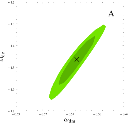
Assuming a flat geometry, we consider two cases to obtain the best fit to the EoS of dark matter and dark energy. First in case A, we assume the prior $\Omega_{dm}=0.235$ (Hinshaw et al., 2012) and we consider as free parameters $h$, $\omega_{dm}$, and $\omega_{de}$. The constraints for case A are given in Table LABEL:tab:table01 using different data sets. The best fit with $\chi^{2}_{min}=664.56$ derived from the joint analysis including all data sets is $h=0.61$, $\omega_{de}=-0.5$, and $\omega_{dm}=-1.46$ with confidence contours at $68.27\%$ and $95.45\%$ shown in the first panel of Figure 1. Furthermore, we consider a second run – which we called case B – in which $\Omega_{dm}$ is also considered a free parameter, whose results are displayed also in Table LABEL:tab:table01. Although the best fit parameters point out towards a negative value for $\Omega_{dm}$ using $H(z)$ and $H(z)+$SNIa, this behavior does not shows up once we include BAO data. The best fit with $\chi^{2}_{min}=664.94$ derived from the joint analysis including all data sets is $\Omega_{dm}=0.22$, $h=0.62$, $\omega_{de}=-0.5$, and $\omega_{dm}=-1.45$. Notice the constraints are very similar in both cases.

Table 1: The best fit values for the free parameters using several data sets in a flat universe. We also show the $\chi^{2}_{min}$ of the fit divided by the effective degrees of freedom.

Case	$\chi^{2}_{min}/d.o.f.$	$\Omega_{dm}$	$h$	$\omega_{dm}$	$\omega_{de}$
$H(z)$
A	$15.53/28$	Fixed	$0.72\pm 0.05$	$-0.57\pm 0.12$	$-1.38\pm 0.67$
B	$15.85/28$	$-0.03\pm 0.51$	$0.81\pm 0.01$	$-0.57\pm 0.04$	$-1.65\pm 0.08$
$H(z)$+SNIa
A	$559.90/585$	Fixed	$0.68\pm 0.01$	$-0.48\pm 0.02$	$-0.94\pm 0.07$
B	$558.82/585$	$-0.25$	$0.68$	$-0.33$	$-0.68$
$H(z)$+SNIa+BAO
A	$594.01/591$	Fixed	$0.63$	$-0.41$	$-1.14$
B	$589.81/591$	$0.27$	$0.62$	$-0.41$	$-1.17$
$H(z)$+SNIa+BAO+CMB
A	$664.56/594$	Fixed	$0.61$	$-0.5$	$-1.46$
B	$663.94/594$	$0.22$	$0.61$	$-0.5$	$-1.45$

Figure 1: Confidence contour at $1\sigma$ and $2\sigma$ for case A (left panel) and case B (right panel) using all data described in Table 1. The cross indicates the best fit.

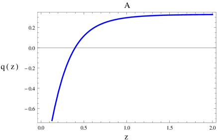
This means we can fit the observational data without using an explicit cosmological constant, as was stressed in Zhang:2010iz , Cardenas:2013ela . Actually, reconstructing the deceleration parameter as a function of redshift $q(z)$ (see Fig. 2) we conclude that this model describes an accelerated expansion without a cosmological constant. The transition of a decelerated phase to an accelerated phase occurs at $z\sim 0.4$.

Figure 2: The deceleration parameter reconstructed from the best fit for case A (left panel) and case B (right panel) using all data.

Figure 3: Analytic solutions (Semi-holographic model including the radiation component) of the energy densities, $\rho_{de}$ (red solid line) and $\rho_{dm}$ (blue dashed line) as a function of redshift, using the best fit values for the case A (left panel) and case B (right panel) using all data. Notice how $\rho_{de}$ falls to negative values near $z\simeq 0.25$.

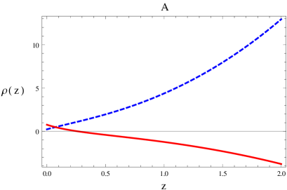
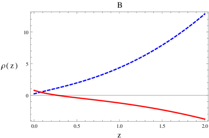
However, as we have already found in the previous work Cardenas:2013ela , it seems that this model presents a fatal failure since there is no chance to satisfied the weak energy condition, because the energy density related to dark energy becomes negative after a fraction of the redshift. In fact, this can be viewed from the explicit solution that we have found, expressed by equation (Semi-holographic model including the radiation component). Based on the best fit values found above, we have plotted the energy densities as a function of redshift in Figure 3, where it is clear that although both energy densities are positive at $z=0$, i.e today, one of them (in this case $\rho_{de}$) falls below zero near $z\simeq 0.25$.

It is interesting to note that this result is not exceptional of this work. Actually in Cardenas:2014jya it was shown evidence that relates the tension between low redshift data and those from CMB, with a preference for evolving DE models showing a decreasing DE density evolution with increasing redshift. This results is also consistent with the recent BAO measurement of BOSS DR11 Delubac:2014aqe , which shows the data prefers a decreasing DE density with increasing redshift. Although this situation looks quite strange since never has been measured a negative energy density, and it is possibly that this case represents an unphysical situation in the sense that it may violate the second law of thermodynamics 2ndLaw (although it can be violated FT ), it is still exist the possibility that a negative energy density studied in a background of a FLRW metric results interesting rhonegative . This could be carried out since the energy conditions in relativity need only be satisfied on a global scale, or on an average measure Ford . It might be interesting to address these issues deeply, in the sense that these energy forms may describe cosmologically interesting scenarios.

In this paper we have reviewed the semi-holographic model presented by Zhang, Li and Noh Zhang:2010iz plus radiation. From this, we have found the analytical solutions to the dynamical system generated by this model, Eqs. (Semi-holographic model including the radiation component), finding accelerated expansion without a cosmological constant. Also, we have studied the stability of the system, which drive us to impose constraints on the EoS parameters, $\omega_{dm}$ and $\omega_{de}$, Eq. (15). Based on this analysis, we determine the allowed region in parameter space to get stable solutions, which does not agree with those mentioned in Zhang:2010iz (see eqs. (23) and (24) in this reference). The analytical solution of the model was also tested against the latest available observational data from Supernovas Ia, which is a set of $580$ points for the module distance.