Super-Sample Signal
Abstract
When extracting cosmological information from power spectrum measurements, we must consider the impact of super-sample density fluctuations whose wavelengths are larger than the survey scale. These modes contribute to the mean density fluctuation in the survey and change the power spectrum in the same way as a change in the cosmological background. They can be simply included in cosmological parameter estimation and forecasts by treating as an additional cosmological parameter enabling efficient exploration of its impact. To test this approach, we consider here an idealized measurement of the matter power spectrum itself in the CDM cosmology though our techniques can readily be extended to more observationally relevant statistics or other parameter spaces. Using sub-volumes of large-volume -body simulations for power spectra measured with respect to either the global or local mean density, we verify that the minimum variance estimator of is both unbiased and has the predicted variance. Parameter degeneracies arise since the response of the matter power spectrum to and cosmological parameters share similar properties in changing the growth of structure and dilating the scale of features especially in the local case. For matter power spectrum measurements, these degeneracies can lead in certain cases to substantial error degradation and motivates future studies of specific cosmological observables such as galaxy clustering and weak lensing statistics with these techniques.
I Introduction
The statistical properties of large scale structure provide a wealth of cosmological information on fundamental physics, including cosmic acceleration, neutrino masses and inflation. The simplest statistic is the two-point correlation function or power spectrum of the matter density field which underlies observables such as weak lensing and galaxy clustering. To extract cosmological information from the power spectrum of upcoming wide-area galaxy surveys (e.g. Takada et al. (2014)), we need to properly model its own statistical properties, one of which is the impact of modes whose wavelengths are larger than the survey scale, the so-called super-sample modes.
While these super-sample modes are not directly observable, they impact the evolution of sub-sample modes in an observable way due to nonlinear mode coupling (Hamilton et al., 2006; Sefusatti et al., 2006; Hu and Kravtsov, 2003; Takada and Bridle, 2007; Takada and Jain, 2009; Sato et al., 2009; Takahashi et al., 2009; de Putter et al., 2012; Schneider et al., 2011; Kayo et al., 2013; Takada and Spergel, 2013; Takada and Hu, 2013; Li et al., 2014; Schaan et al., 2014). Ref. Takada and Hu (2013) developed a simple, unified approach that describes the impact of the super-sample modes as the response of the power spectrum to a change in the mean density in the finite-volume region. Ref. Li et al. (2014) then utilized the so-called separate universe approach to calibrate this response in -body simulations. Here, the mean density fluctuation is absorbed into a change in cosmological parameters (e.g. Tormen and Bertschinger (1996); Cole (1997); Sirko (2005); Baldauf et al. (2011); Gnedin et al. (2011)). The separate universe approach is also useful for gaining a physical understanding of the response. In a coherently overdense region structure grows more quickly and regions expand less quickly. The response is therefore a change in the amplitude or growth of structure and in the scale or dilation of features in the power spectrum.
The impact of the mean density fluctuation can also be viewed in two ways: as additional noise due to its stochasticity, or as additional signal from which the mean density in a given volume may be recovered Takada and Hu (2013). In the former view, the super-sample effect introduces a covariance to power spectrum estimates since each realization of coherently changes the power spectrum according to the calibrated response. Ref. Li et al. (2014) used the covariance matrix of power spectra in subsampled simulations to verify the separate universe response itself.
Here we develop the alternative view that in each realization the super-sample effect biases the measured power spectrum or equivalently introduces an extra parameter, , upon which it depends. The mean density fluctuation leaves a signal in the power spectrum which can be used to recover its value providing constraints on super-sample modes that are not directly observable in the survey (see also Takada and Spergel (2013); Chiang et al. (2014)). Moreover, this view facilitates studies of the impact of super-sample modes on cosmological parameter estimation by treating the two on an equal footing.
While here we only test this view in the idealization that the matter power spectrum is directly observed, these ideas can be readily extended to more observationally relevant power spectrum observables once their response to is calibrated.
The structure of this paper is as follows. In § II we review the super-sample effects on the power spectrum and test its interpretation as signal by explicitly constructing an estimator of the mean density fluctuation in simulations. In § III we study the similarities between the power spectrum response to the mean density fluctuation and to cosmological parameters which propagate into parameter degeneracies in the Fisher information matrix. We discuss these results in § IV. Appendix A provides details of the simulations and the numerical techniques.
II Super-sample signal
In § II.1, we first briefly review the impact of super-sample modes on the power spectrum covariance which was developed in Refs. Takada and Hu (2013); Li et al. (2014). Next we show the effect can alternately be treated as a signal that allows us to construct an unbiased minimum variance estimator of the mean density fluctuation in § II.2. We test this estimator against cosmological simulations in § II.3 and show that its statistical properties are well-characterized by the separate universe response of the power spectrum to the mean density and the covariance of the power spectrum in the absence of the mean density mode.
II.1 Super-sample modes
In this section we characterize the effect of super-sample modes on power spectrum measurements in a finite survey volume in a manner that brings out their role as both signal and noise. Let us denote the average density fluctuation in the survey region from these modes as and assume that the measurement of the power spectrum of sub-survey modes is sample variance limited. Let us bin these measurements into a data vector
| (1) |
and consider the impact of on the mean and covariance of these data. We use the dimensionless power spectrum since it is independent of the units with which the wavenumber is measured and thus allows a cleaner separation of effects on the amplitude and scale of structure (see Ref. Li et al. (2014)).
Even if we define an estimator which yields the true power spectrum when averaged over realizations of all modes, including the super-sample ones
| (2) |
the average over realizations of different sub-survey modes at fixed , which we denote by , is biased
| (3) |
Here we have linearized the response of the power spectrum assuming
| (4) |
As demonstrated in Ref. Li et al. (2014) through its effects on the power spectrum covariance below, we can use the separate universe approach to calibrate the power spectrum response, , for a given fiducial cosmological model. In this approach the mean density fluctuation of the survey is absorbed into the local background density by redefining cosmological parameters.
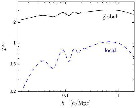
Fig. 1 summarizes the results for the CDM model (see Tab. 2) at using -body simulations to calibrate the response deep into the nonlinear regime. Note that the technique itself is more general than this particular implementation. Given a state-of-the-art simulation that includes baryonic effects, e.g. star formation and feedback Rudd et al. (2008); van Daalen et al. (2011), the impact of super-sample modes can still be calibrated by runs where the background parameters are changed to absorb .
These results apply to power spectrum measurements where the global mean density is known through cosmological parameters, e.g. in the case of weak lensing power spectra. If the power spectrum is estimated with respect to the local mean density within the survey region, which is the case for galaxy surveys, the relevant observable is
| (5) |
where denotes the survey volume or window here and below. The power spectrum response is therefore modified to be
| (6) |
Because the formalism for super-sample effects is otherwise identical, we use the term “local” data or response when replacing the “global” versions of Eqs. (4) and (5), in relevant formula below. Both responses are shown in Fig. 1.
Since is a random zero mean variable, its variance turns into a covariance of the power spectrum estimators. In this sense the super-sample effect contributes as additional noise. We can model this noise by treating the bias as a purely systematic additive shift in the power spectrum per realization
| (7) |
The covariance matrix of the power spectrum data is then given by
| (8) |
where is the variance of the mean density field in the survey window, defined as
| (9) |
Here is the survey volume and is the survey window function which acts as a low pass filter. For a sufficiently large survey volume, the super-sample modes are in the linear regime and therefore can be accurately calculated with the linear power spectrum either by explicit computation of Eq. (9) or Gaussian realizations of the linear density field. The matrix in Eq. (8) is defined as
| (10) |
Note that this is the covariance of the power spectrum estimators in the absence of the super-sample effect. It can be readily calibrated from a suite of small-volume -body simulations for a given cosmological model Scoccimarro et al. (1999); Meiksin and White (1999) (see Appendix A and Ref. Li et al. (2014) for implementation specifics). The sum of the two contributions of Eq. (8) reproduces the super-sample covariance derived in Ref. Li et al. (2014) from trispectrum considerations.
An alternate model would be to consider the bias in the power spectrum estimators to be multiplicative with respect to ,
| (11) |
This model yields an additional contribution to the second term of Eq. (8)
| (12) |
and hence only a small change for well measured bins where the covariance is much smaller than the product of the means. We hereafter adopt the additive model.
II.2 Signal vs. noise
In a given realization of the survey volume, the super-sample effect systematically changes the power spectrum of sub-survey modes just like a cosmological parameter . Indeed, in the additive model of Eq. (7), the analogy is precise: is simply a parameter that changes the mean power spectrum
| (13) |
Thus the data in the presence of has the same statistical properties as in its absence. They are both drawn from a distribution with covariance and only the mean is shifted. Parameter estimation then proceeds in the usual way by treating as a parameter . For example, the posterior probability of model parameters including can be estimated using Markov Chain Monte Carlo techniques based on the likelihood function constructed from the covariance matrix with the model parameterized by . In this view, the super-sample effect is a signal which allows the mean density fluctuation to be recovered rather than a source of additional noise.
To test this interpretation with simulations, we can construct an explicit estimator of based on linear response. Here we shall assume that cosmological parameters are fixed and hence suppress their appearance in the expressions. A general unbiased linear estimator of takes the form
| (14) |
where the weight
| (15) |
is constrained by the condition . The remaining freedom in choosing the weights is fixed by minimizing the variance of the estimator
| (16) |
subject to the Lagrange multiplier constraint yielding
| (17) |
and
| (18) |
If instead of the additive bias model, the multiplicative bias model of Eq. (11) is correct, this estimator remains unbiased but its variance changes. Thus comparing the predicted variance from Eq. (16) with the variance obtained from simulations tests the accuracy of our additive model of super-sample effects as well as that of the response and covariance calibration.
II.3 Density estimation
In this section, we test the estimator with large-volume simulations where the true mean density fluctuation is known in each subvolume of the simulation. We summarize here the relevant simulation details presented in Appendix A. Specifically 7 large-volume simulations, each with a box length are divided into a total of subvolumes of size Mpc each. For reference the variance of the mean density fluctuation of the subvolumes is
| (19) |
which matches well the computation from Eq. (9), . We measure the power spectrum in each subvolume separately. Note that this power spectrum is of the density fluctuation from the large-box mean and hence characterizes the “global” data in the language of §II.1. For the “local” data, we use the true average density in the subvolume to rescale the global data according to Eq. (5).
To calibrate the mean power spectrum and the covariance matrix , we run another suite of small box simulations each of the same size as the subvolume. All power spectra are binned in -bins per decade and we utilize measurements out to Mpc-1 up to which we verified the response calibration is accurate to several percent or better, based on higher-resolution simulations (Li et al., 2014).
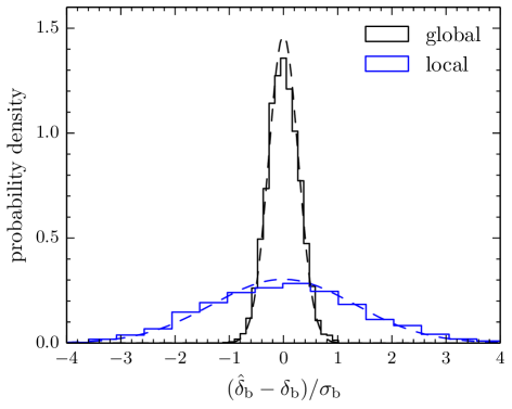
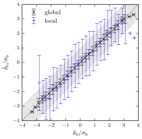
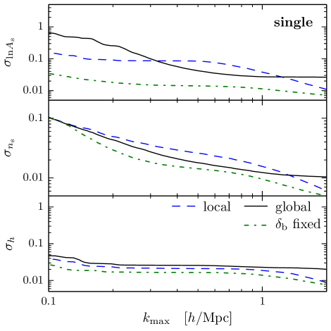
From , , and we form the estimator of Eq. (14) for both the global and local cases and compare it with the true value in each of subvolumes. Fig. 2 shows the results binned in with width . In both the global and local estimations, there is no trace of a bias in the estimator to a small fraction of its standard deviation. Moreover, in Fig. 3 we test the predicted distribution of the estimator combining all bins with the prediction from Eq. (16) for the variance under the assumption of a Gaussian distribution. The agreement in both cases is very good. For a more quantitative assessment we measure the variance of the estimator with our samples in the usual way
| (20) |
The result is for the global case and for the local case. In both cases the result is only larger in standard deviation than the prediction of Eq. (16). Even in the local case where the standard deviation is comparable to there is non-negligible extra information provided by the estimator.
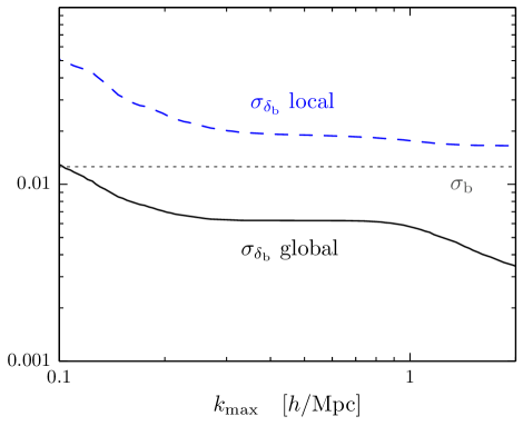
These results validate the use of our additive model to predict the impact of the super-sample effect in other cases of interest. In Fig. 4, we use this model to explore the dependence of the standard deviation of the estimator on the maximum used. Note that in the local case, is only a weak function of . This is because, the intrinsic covariance between bins induces very similar changes to the power spectrum as local for Mpc-1. The difference in shape between the local and global responses causes an improvement in the standard deviation of the latter for Mpc-1.
The above results apply to estimates of when all other parameters that change the power spectrum are known a priori. With joint estimator of parameters from the survey, the mode will degrade results on cosmological parameters and vice versa if their impact on the power spectrum is sufficiently similar to cause degeneracies.
Finally in the additive model, the scaling of these results with the volume of the survey is also simple. Since characterizes the covariance of subsurvey modes in the absence of the super-sample effect, it scales with volume as
| (21) |
where , the volume of the simulation test. Hence
| (22) |
for any parameter estimated from power spectra data including . The ratio does in general depend on volume. However in CDM the quantity varies weakly with , typically by across a . Thus we expect that the relative impact of the super-sample effect will be only weakly dependent on volume for the cubic geometry we consider. In Ref. Takada and Hu (2013) it was also shown that for a cylindrical geometry the scaling holds although itself is smaller for the same volume.
III Parameter forecasts
In this section we use the Fisher information matrix formalism to study the impact of the super-sample effect on cosmological parameter estimation in the idealized context of direct matter power spectrum measurements. After defining the Fisher matrix in § III.1, we study similarities in the power spectrum response between the super-sample mode and cosmological parameters in § III.2. These similarities lead to degeneracies which degrade errors when parameters are jointly estimated in § III.3 and are themselves limited by prior information on the variance of the super-sample mode III.4.
III.1 Fisher matrix
As discussed in §II.2, the additive model can be thought of as an additional parameter of the model power spectrum so that the full parameter vector is , where are cosmological parameters. In the Fisher approximation, the information from the power spectrum mean is added to any prior information on the parameters,
| (23) |
where
| (24) |
The inverse Fisher matrix is an approximation to the covariance matrix of the parameters
| (25) |
To make contact with §II.3, note that in the limit that the parameter space includes only and there is no prior information on it, Eq. (25) yields the variance of the estimator given in Eq. (18). This is because the Fisher approximation involves the same linearization of the response to the parameters that permits the construction of a linear minimum variance unbiased estimator. With additional parameters and no external prior, degeneracies where the errors strongly covary appear if the responses take a similar form. Thus to understand the impact of super-sample modes on parameter estimation we must compare the various responses .
III.2 Parameter responses
Given that the separate universe technique described in §II.1 and detailed in Ref. Li et al. (2014) involves modeling the super-sample effect by changes in background cosmological parameters, we expect the response to and cosmological parameters will contain similarities that can create parameter degeneracies. Namely, these parameters change the amplitude of power in the spectrum and the scale at which features like baryon acoustic oscillations (BAO) appear. We will call these effects growth or “g” and dilation or “d” respectively.
Let us begin by examining this decomposition for and a power spectrum measurement with respect to the local mean density of the survey, defining
| (26) |
Here and below we omit the -bin index where no confusion should arise. The first term is due to the enhancement of the growth of structure in a coherently overdense region. Absorbing this fluctuation into a redefinition of the background implies a change in the linear growth function of density fluctuations with respect to the local mean density Baldauf et al. (2011)
| (27) |
Hence, with this normalization, .
The second term of Eq. (26) is due to the fact that an overdense region expands less quickly than the global universe. This changes the comoving scale of physical features in the power spectrum according to a dilation template
| (28) |
The factor of arises since an equal time comparison is at equal physical mean density and so the scale factor is adjusted by . By removing this rescaling with a choice of simulation box size introduced in Ref. Li et al. (2014) (see also Appendix A), we can determine independently of the full response as shown in Fig. 6. The difference between these responses gives the dilation template which is compared with the -derivative of the mean power spectra in Fig. 7. The agreement is good and as discussed in the Appendix, the response difference provides a more accurate way of calibrating dilation than differencing noisy power spectrum data.
Finally, when referenced to the true global mean density, the response becomes (see Eq. 6)
| (29) |
Note that the additional factor flattens the response of the power spectrum as shown in Fig. 1. We shall see that this addition is important for understanding parameter degeneracies (cf. Mohammed and Seljak (2014)).
Now let us compare this response with those of cosmological parameters. The full set of flat CDM parameters are which jointly define the primordial curvature power spectrum
| (30) |
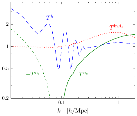
the baryon density ; the cold dark matter density and the dimensionless Hubble constant . The parameters and are well determined by the cosmic microwave background (CMB) data and additionally are not degenerate with pure growth and dilation due to the changes in the BAO and matter radiation equality features that they induce. We therefore study responses to changes in the parameter set and keep the remaining parameters fixed to their fiducial values. We calibrate each response function as discussed in Appendix A.2.2 and show the results in Fig. 5.
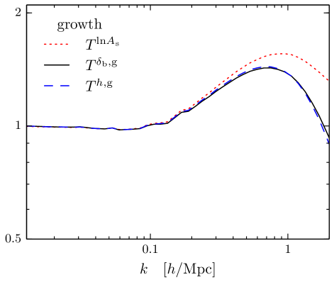
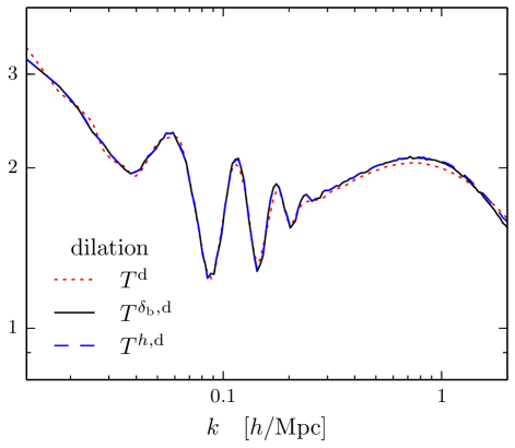
The response to shares the same features as . Since is varied at fixed and in a flat universe its impact on the power spectrum in the linear regime at a fixed scale in Mpc comes solely from changing the growth function due to the change in . However because observations at determine a scale in Mpc-1, observable features in the power spectrum shift. This is the same effect that allows BAO to measure at or the expansion rate and angular diameter distance at higher redshift. The result is that the response can be decomposed as
| (31) |
For reference, in the chosen cosmology . As shown in Fig. 6, the growth pieces of the and responses are nearly indistinguishable. Likewise, defining the dilation piece as the difference of these responses agrees with the dilation defined from and the -derivative of the mean power spectrum as shown in Fig. 7. In an extended parameter space, we expect the response to parameters such as the dark energy equation of state or curvature can be modeled accurately with and their impact on the linear growth function .
Next directly controls the amount of power in the spectrum at the initial epoch. At a change in and a change in growth can produce the same linear power spectrum and hence in the linear regime the two responses are indistinguishable. In Fig. 6 we compare these response and show that they begin to differ in the nonlinear regime. If the nonlinear power spectrum were a functional of the linear power spectrum then the responses would be identical. For example, in a halo model description, if the mass function were universal and the scale radii of halos were fixed then the linear power spectrum determines the nonlinear power spectrum directly with no further reference to the past history of structure formation. We have verified that the differences in response are qualitatively modeled by a change in concentration of halos with respect to a fixed scale 111Fixed as opposed to a parameter dependent scale such as the virial scale. For example where the spherical overdensity is 180 times the mean matter density.. The concentration of halos retains information about the mean density of the Universe at their formation epoch, and so one would not expect a change in the initial conditions and late-time growth that leaves the linear power invariant to yield the same concentration. In principle, then is not degenerate with other parameters associated with growth. In practice, uncertainty in the concentration-mass relation due to baryonic physics can restore this degeneracy.
Small changes in the tilt can also restore this degeneracy across a limited range in . Fig. 5 also shows the response to tilt, which changes the power spectrum in opposite directions around the pivot point MpcMpc-1. Given the greater statistical power of measurements in the nonlinear regime, a small amount of tilt can compensate the differences due to changes in the concentration.
In summary, the response functions show that for power spectrum measurements with respect to the local mean, there are 3 parameters whose power spectrum response is characterized mainly by linear combinations of two templates, and once minor changes in tilt or halo concentration are factored in. We therefore expect a strong degeneracy in the local case. For power spectra measured with respect to the global mean, the addition of 2 to the response breaks this degeneracy yielding three templates for three parameters. We shall now see that these features are reflected in the forecasted parameter errors.
III.3 Parameter constraints without prior
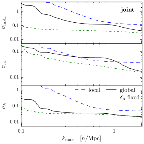
We begin with parameter constraints for the case where there is no external prior on so that any information about it must be recovered from the power spectrum measured by the survey. Fig. 8 shows an overview of the impact of marginalizing on cosmological parameter estimation. The left panel shows the impact on the 3 cosmological parameters considered one at a time with the other 2 fixed whereas the right panel shows the result with the other two marginalized. In the former case, the degradation is the most severe when the two templates are most similar. For example in the global case, the flattening of the response in the nonlinear regime relative to local in Fig. 1 makes it more similar to around Mpc-1 and causes a larger degradation in errors for such choices of . Parameter degeneracies also increase the importance of having a sufficiently large to distinguish the responses compared with a naive quantification of information through Rimes and Hamilton (2005, 2006) (see also Takada and Jain (2009); Sato et al. (2009)).
Similar statements apply for the case where the two other cosmological parameters are also marginalized. Here what is important for determining degeneracies is whether a linear combination of the four responses can compensate each other. From Fig. 8 (right) we see that the flattening of the global vs. local response now has the opposite effect on . By Mpc-1 most degeneracies are broken for the global case whereas they remain strong and impact all three cosmological parameters in the local case.
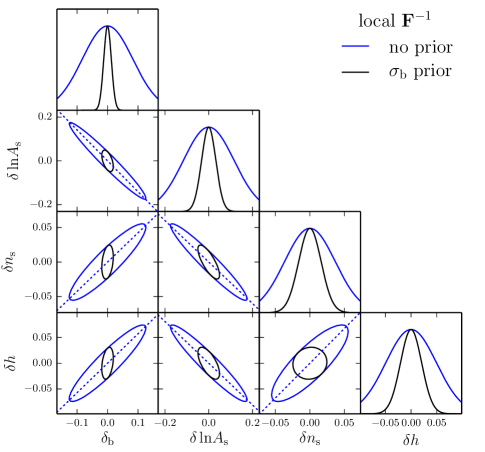
To see how these results arise geometrically, we show various 2D 68% confidence regions for the 4 parameters for the local case in Fig. 9 (left) with Mpc-1. In particular, the contours involving show a strong degeneracy with all three of the other parameters. This implies that without a prior on , constraints on cosmological parameters will be severely degraded by marginalizing . This degradation is quantified in Tab. 1 (see Appendix A.3 for details and notation). With the Fisher matrix, we can use the eigenvector with the largest variance to identify the degenerate direction
| (32) |
where we have normalized the vector such that the estimator of this mode has unit variance. This direction is displayed as the dashed lines in Fig. 9 (left).
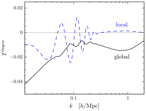
Fig. 10 shows the response of the power spectrum to this combination. This linear combination nulls the response in the nonlinear region where changes in the tilt and halo concentration can compensate each other. The change in tilt implies a change in the linear regime which variations in partially compensate at the expense of leaving a residual response in the BAO scale.
| local | global | |||
|---|---|---|---|---|
| parameter | no prior | prior | no prior | prior |
| 4.14 | 1.17 | 1.51 | 1.24 | |
| 2.37 | 1.05 | 1.09 | 1.04 | |
| 2.54 | 1.06 | 1.10 | 1.04 | |
| max, | 5.02 | 1.24 | 4.34 | 2.91 |
| 4.14 | 1.09 | 1.51 | 1.15 | |
| 2.37 | 1.03 | 1.09 | 1.03 | |
| 2.54 | 1.03 | 1.10 | 1.03 | |
| max, | 5.02 | 1.13 | 4.34 | 2.37 |
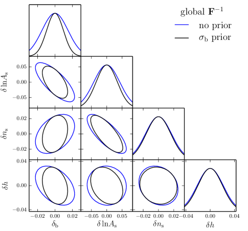
Next in Fig. 9 (right) we show the 2D error contours for the global case. As discussed in the previous section, the change in the response from the local case eliminates the near degeneracy provided by the growth and dilation responses. Consequently the degradation in parameter errors from marginalizing is much smaller as shown in Tab. 1. The largest degradation occurs for and involves mainly the direction
| (33) |
Fig. 10 shows that this direction does not allow an approximate nulling of the response in the nonlinear region. Instead it yields a flat response in the nonlinear region which no longer requires significant variations in to compensate in the linear regime.
Although these degeneracy studies, which identify the worst constrained directions, reveal the overall impact on the individual cosmological parameters, it is also interesting to consider the impact of marginalizing on the best constrained directions. For example, if the CMB or other cosmological probe constrains a different combination of these parameters and breaks the degeneracy, then the impact of the best constrained directions may be revealed. Moreover, the impact of marginalizing is generally larger on the best rather than worst constrained directions. In Appendix A.3, we formalize these statements by identifying the combination of cosmological parameters whose errors are most degraded by marginalizing ,
| (34) |
which in practice are in directions very similar to the best constrained direction without marginalization
| (35) |
especially in the global case. Here again we normalize each mode so that its estimator has unity variance, conditional on held fixed. The amount of the degradation is numerically equal to that on upon marginalizing over cosmological parameters. In Tab. 1 we compare the various degradation in errors. Note that even in the global case, the maximal degradation is large and comparable to the local case.
Finally given that the covariance matrix scales with survey volume according to Eq. (21), we can account for a change in survey volume by simply rescaling all parameter errors according to Eq. (22) so that the relative impact of remains the same.
In summary, even though the local case involves a smaller response to , it can have a much bigger impact on cosmological parameter estimation compared with the global case due to the ability to construct near perfect degeneracies in the nonlinear regime. On the other hand, errors in the combination of cosmological parameters along the direction that is best constrained without are substantially degraded in both cases.
III.4 Parameter constraints with prior
If the linear power spectrum were perfectly predicted by external information on cosmological parameters such as the CMB measurements, then we would possess prior knowledge that is distributed as a Gaussian with variance . In this limiting case
| (36) |
where is the Kronecker delta. Here we use Eq. (9) to evaluate . In practice, cosmological parameter uncertainties should be propagated into this prior but this simple prior is useful to study as a best case scenario. Note that the view of super-sample effects as signal makes it simple to incorporate uncertainties in as opposed to the excess covariance approach where it would enter through the cosmological parameter dependence of the covariance matrix.
The impact of this prior is qualitatively different in the local and global cases. In the local case, with all 4 parameters jointly estimated, intrinsic parameter degeneracies are so strong that the net degradation in parameter estimation from marginalizing is prior limited as shown in Fig. 9 (left) and Tab. 1. For the global case, the degradation is only marginally changed by the prior. In both cases, with the prior, the remaining impact of marginalizing is mainly on and represents approximately a factor of degradation in its errors.
The reason that these degradations are small in both cases is the remaining degeneracies among the cosmological parameters themselves come to dominate the parameter errors. This fact however does not mean that marginalizing has little effect on combination of cosmological parameters that are well constrained in its absence. The direction of maximal degradation is the same with or without the prior and so is close to the best constrained direction in Eq. (35). In the global case, this degradation is nearly a factor of 3 and is substantially larger than the local case. This degradation can be important for errors on individual cosmological parameters if other measurements break the intrinsic cosmological parameter degeneracies.
Finally, with a prior, parameter errors do not simply scale with volume as unless . To test the impact of volume scaling we consider a case where the volume is increased by . In this case is reduced by a factor of . For cases that are not limited by the prior, the volume scaling of ensures that the degradation factors are the same. In general for CDM, increasing the volume tends to slightly strengthen the relative impact of the prior.
IV Discussion
Super-sample density fluctuations systematically change the observable power spectrum of sub-sample modes. In this paper, we have developed and tested the interpretation of this effect as a signal due to the dependence of the observed power spectrum on the mean density fluctuation in the survey volume . This dependence can be calibrated efficiently by using the separate universe technique that absorbs the fluctuation into a change in the background parameters.
This interpretation has the advantage that the effect can be incorporated into parameter estimation without modification of traditional procedures or pipelines. The form of the likelihood of the power spectrum data as a function of the model takes the same form except that the model gains a parameter in addition to cosmological parameters. Its impact on cosmological parameter estimation comes through parameter degeneracies. Contrast this with the alternate but equivalent view that when ensemble averaged over many realizations of the survey volume and , the effect induces a covariance in the power spectrum that modifies the form of the likelihood function.
The super-sample signal allows itself to be estimated from power spectrum data. The amount of information on depends on whether the power spectrum is measured with respect to the global or local mean density, which is relevant, e.g., for weak lensing or galaxy clustering, respectively. For a wide range of survey volumes, the global case contains substantial extra information in the nonlinear regime on top of the prior expectation that it be limited by the rms predicted by linear theory. For the local case, the extra information is comparable to the prior for Mpc-1.
If cosmological parameters are jointly estimated, this extra information can be lost to degeneracies. Likewise, marginalization of can degrade errors on cosmological parameters. The degradation takes on different values depending on the the parameter space and priors considered, whether the local or global power spectra are used, and the maximum wavenumber utilized. In general, the strongest degeneracies arise from compensated changes in the growth of structure and dilation of features induced by the parameters, which provides a physical basis for which to extend our results beyond the CDM parameter space. Without prior information on , the degradation of errors for the local case can be more than a factor of 4 for Mpc-1 and likewise in the global case but only for the combination of cosmological parameters that is best measured in the absence of and maximally degraded by its marginalization. Even with a prior that reflects perfect knowledge of the linear power spectrum, the maximal degradation in the global case can reach a factor of 2–3. Fortunately all of these cases and more can be simply and rapidly considered given a single calibration of the power spectrum responses.
While we have only considered the effects on the matter power spectrum through -body simulations in CDM, our separate universe and growth-dilation techniques can be extended to other parameter spaces or observables and can incorporate baryonic effects and galaxy formation. While other uncertainties in modeling the data, e.g. redshift space distortions and galaxy bias for galaxy surveys, may dominate the error budget for current measurements, the super-sample mode provides an intrinsic limitation to extracting cosmological information that is degenerate with its effects.
Acknowledgments.– We thank M. Becker, M. Busha, B. Erickson, G. Evrard, N. Gnedin, A. Kravtsov, D. Rudd, R. Wechsler, and the University of Chicago Research Computing Center for running, storing, and allowing us to use the large-volume simulations in this study. We also thank M. Becker, D. Rudd., N. Gnedin, A. Kravtsov and F. Schmidt for useful discussions. YL and WH were supported by U.S. Dept. of Energy contract DE-FG02-13ER41958 and the Kavli Institute for Cosmological Physics at the University of Chicago through grants NSF PHY-0114422 and NSF PHY-0551142. MT was supported by World Premier International Research Center Initiative (WPI Initiative), MEXT, Japan, by the FIRST program “Subaru Measurements of Images and Redshifts (SuMIRe)”, CSTP, Japan, and by Grant-in-Aid for Scientific Research from the JSPS Promotion of Science (Nos. 23340061 and 26610058). This work was also supported in part by the National Science Foundation under Grant No. PHYS-1066293 and the hospitality of the Aspen Center for Physics, where this work was completed. Plots in this work are made with matplotlib Hunter (2007).
Appendix A Numerical Implementation
In this Appendix we provide details on various numerical calculations in the main paper. In § A.1, we describe the cosmological simulations used in the super-sample signal studies. We calibrate the power spectrum response to various parameters in § A.2. In § A.3, we establish the formalism for calculating the degradation of parameter errors upon marginalizing over .
A.1 Simulations
| 0.286 | 0.047 | 0.7 | 0.96 | 0.82 |
Here we summarize the salient features of the simulations and power spectrum analysis from Ref. Li et al. (2014) and used in § II to test super-sample effects with subvolumes of large-volume simulations. For the large-volume simulations, we take a suite of 7 realizations of the fiducial cosmology given in Tab. 2, originally made for the Dark Energy Survey. Each of these has a box length evolved from initial conditions at that are provided by CAMB Lewis et al. (2000); Howlett et al. (2012) and 2LPTIC 222http://cosmo.nyu.edu/roman/2LPT/, using L-Gadget2 Springel et al. (2005) with particles and (Tree-)PM grid. We then assign the particles to a grid with a cloud-in-cell (CIC) scheme, before subdividing each large box into subvolumes of size
| (37) |
for a total of subboxes.
In each subvolume, we extract the mean density fluctuation and the power spectrum by FFT. For the power spectrum, we then deconvolve the CIC window and bin the result to 80 logarithmically spaced -bins per decade to form . Each bin is positioned at the average weighted by the number of modes. This binning scheme is used throughout the paper.
To calibrate the mean power spectrum and its covariance matrix , in the absence of , we use the same number of simulations of the same size as the subboxes but with particles and (Tree-)PM grid. We measure the power spectrum of each small-box simulation in the same way with a grid. All the numerical settings match the scaling of the large box dimensions except for the (Tree-)PM grid.
The mean power spectrum of the subboxes differs from that of the small boxes in two ways. On large scales the difference is dominated by convolution bias from the subbox window, and on small scales there is a difference due mainly to using different resolutions for the (Tree-)PM grid in simulations. We debias the estimator as in Ref Li et al. (2014) by rescaling
| (38) |
where we have defined
| (39) |
as the average over the samples. Thus
| (40) |
For the power spectra referenced to the subbox mean
| (41) |
where is the average density fluctuation in the same box.
Next we estimate the covariance matrix in the absence of as
| (42) |
Finally unless otherwise specified, the simulations used to construct the response functions in the next section follow the prescription for the small box simulations in order to preserve the same mass and force resolution.
A.2 Response calibrations
In this section we provide some detail on the calibration of the power spectrum response to and the cosmological parameters. We review the response calibrated in Ref. Li et al. (2014) and illustrate the cosmological parameter calibration with as it demonstrate all the important concept and techniques.
A.2.1 response
Following the separate universe technique developed in Ref. Li et al. (2014) (see also Sirko (2005); Baldauf et al. (2011); Gnedin et al. (2011)), a nonzero mean density fluctuation at can be absorbed into the background by a redefinition of the cosmological parameters compared to those of a global CDM universe
| (43) |
where the and the linear growth function is normalized as
| (44) |
Note that even if the global universe is flat, the separate universe would have a nonzero spatial curvature . Finally, as discussed in § III.2, the scale factor associated with a given value of in the global cosmology is shifted by
| (45) |
in the separate universe. For example, at in the global universe, in the local universe.
With the separate universe cosmological parameters set, we conduct -body simulations to calibrate the response of the power spectrum by finite difference of models with evaluated at . Here and below we always difference simulations with the same initial seeds to suppress the stochasticity from sample variance. Given that the mean density of the separate universe is reinterpreted as the local density of the finite survey, power spectra extracted from these simulations are always referenced to the local mean, in Eq. (5).
To calibrate the growth response , we fix the simulation box in comoving Mpc and difference the results from . This procedure only includes the impact of on the growth of structure and omits the fact that due to the difference in redshift, the physical scale associated with a given comoving scale differs by the dilation factor. Separately, we also calculate the total response by instead fixing the physical scale in Mpc of the simulations at the final redshift with the same initial seeds in box coordinates. Finally we average over 64 pairs of realizations to reduce the remaining stochasticity to a level that is negligible for our purposes, with standard errors of the mean of a few percent or better, and at sub-percent level in the nonlinear regime.
To test the precision of our results, we have employed simulations with twice the mass and PM resolutions, to verify that at for /Mpc the responses have converged to several percent or better. We refer the readers to Ref. Li et al. (2014) for more details of the calibration pipeline.
With and calibrated from simulations we can construct the dilation response from Eq. (26)
| (46) |
We compare this constructed dilation response in Fig. 7 with the response calibrated directly as the slope of a cubic spline fitted to the mean power spectrum of small box simulations
| (47) |
The differences in fact reflect that the constructed response reduces the stochasticity from sample variance and the sensitivity to systematic changes in the slope from finite resolution. We have verified using higher resolution simulations that the constructed response is both more precise and more accurate than the slope-based response.
A.2.2 response
As an example of cosmological parameter response calibration, we choose here as it demonstrate all the important concept and techniques, including the growth-dilation split, and the test of the linear approximation. We start with the baseline cosmology in Tab. 2 and utilize a suite of 64 simulations from the small box simulations of § A.1. As in the calibration we then simulate pairs of models with with the same seeds to form a triplet of simulations at fixed , , and in a flat universe. We choose in accordance with the confidence limits constrained by Planck and WMAP polarization data.
For the total response , we set the comoving size of simulation boxes in Mpc to be the same, i.e.
| (48) |
whereas for extracting the growth component, we set the box scale in Mpc to be the same
| (49) |
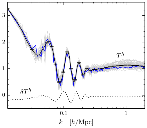
We then difference the binned power spectrum in box coordinates in each case to form the required derivative
| (50) |
For sufficiently small , this finite difference converges to the derivative as required for a Fisher matrix calculation. Each of the 64 pairs provides a separate estimate of the response. In Fig. 11 we show the individual estimates and the mean of the suite . Note that run-to-run deviations from the mean strongly covary across in the nonlinear regime.
Finally, to test the linearity of the response, we calibrate the change in the response from the second derivative
| (51) |
using the averages over the 64 triplets. In Fig. 11, we demonstrate that this second derivative error term . Specifically, in the fully nonlinear regime where the statistical power lies, the error correction is . While we could further reduce this error by choosing a smaller , this test demonstrates that even for current uncertainties on this parameter, the Fisher approximation should suffice.
To test the resolution dependence, we have employed pairs of higher resolution simulations with particles and (Tree-)PM grid to verify that at Mpc-1 our response results have converged to percent level or better.
With both and calibrated in this manner, we can construct the dilation response using Eq. (31),
| (52) |
Similar to the case discussed above, this construction yields a more accurate and precise dilation response than the slope-based response.
The calibration of and are simpler as no scale dilation is involved, so that we can use the same box size for simulations. We take and again according to the CMB prior, and the rest of the procedures are the same as for . For and , the linear response assumption is an excellent approximation, with second order corrections at the percent level or smaller.
A.3 Error Degradation
In the main text, we quote the degradation in the errors in a given cosmological parameter and the maximal degradation for any linear combination of parameters caused by marginalizing . Here we give details for those calculations.
The covariance matrix of cosmological parameters with marginalized is simply the subblock of the inverse Fisher matrix that contains them. We can formalize the extraction of this matrix by defining a projection matrix
| (53) |
where and is the identity matrix. Thus
| (54) |
Conversely, if is fixed then the covariance matrix is instead the inverse of the projected Fisher matrix
| (55) |
In the same linear approximation employed in the Fisher analysis, the deviation in any derived parameter from its fiducial value can be thought of as a linear combination of changes in fundamental parameters,
| (56) |
where Greek indices in this section run over the 3 cosmological parameters and parameter vectors lie in this space. Thus the degradation in errors upon marginalizing is given by
| (57) |
We can most easily study the degradation in errors in a new basis, called the Karhunen-Loève basis. The 3 basis vectors are linearly independent solutions of the generalized eigenvector equation
| (58) |
Note that , the degradation in the variance of a parameter defined by and we can normalize these statistically independent vectors as
| (59) |
These vectors are not typically orthonormal in the usual sense .
The Karhunen-Loève basis is typically used when the two matrices in Eq. (58) are the signal and noise covariance respectively and in that context the eigenvectors are called signal-to-noise eigenvectors. In this case, they represent degradation eigenvectors.
The eigenvalues are particularly easy to find in our case given the relationship between the two matrices implies
| (60) |
or in terms of components
| (61) |
For vectors in the two directions that are orthogonal to , the second term on the left hand side vanishes and . In these directions, marginalization of has no impact since these elements of represent a covariance of the associated direction with . The remaining eigenvector is in the direction of
| (62) |
which is not in general parallel to or orthogonal to the 2D space spanned by the other vectors. Thus the direction of maximal degradation and the combination of cosmological parameters associated with it
| (63) |
is not in general the same as those of maximal covariance or degeneracy. The maximal degradation itself is given by the eigenvalue
| (64) |
and is exactly the degradation in on marginalizing over cosmological parameters. A general linear combination of cosmological parameters suffers a degradation whose value cannot exceed the maximum since it is composed partially of the 2 Karhunen-Loève directions that are not degraded Smith et al. (2006).
References
- Takada et al. (2014) M. Takada, R. S. Ellis, M. Chiba, J. E. Greene, H. Aihara, N. Arimoto, K. Bundy, J. Cohen, O. Doré, G. Graves, J. E. Gunn, T. Heckman, C. M. Hirata, P. Ho, J.-P. Kneib, O. L. Fèvre, L. Lin, S. More, H. Murayama, T. Nagao, M. Ouchi, M. Seiffert, J. D. Silverman, L. Sodré, D. N. Spergel, M. A. Strauss, H. Sugai, Y. Suto, H. Takami, and R. Wyse, PASJ 66, R1 (2014), arXiv:1206.0737 [astro-ph.CO] .
- Hamilton et al. (2006) A. J. S. Hamilton, C. D. Rimes, and R. Scoccimarro, Mon. Not. Roy. Astron. Soc. 371, 1188 (2006), arXiv:astro-ph/0511416 .
- Sefusatti et al. (2006) E. Sefusatti, M. Crocce, S. Pueblas, and R. Scoccimarro, Phys. Rev. D 74, 023522 (2006), arXiv:astro-ph/0604505 .
- Hu and Kravtsov (2003) W. Hu and A. V. Kravtsov, Astrophys. J. 584, 702 (2003), arXiv:astro-ph/0203169 .
- Takada and Bridle (2007) M. Takada and S. Bridle, New Journal of Physics 9, 446 (2007), arXiv:arXiv:0705.0163 .
- Takada and Jain (2009) M. Takada and B. Jain, Mon. Not. Roy. Astron. Soc. 395, 2065 (2009), arXiv:0810.4170 .
- Sato et al. (2009) M. Sato, T. Hamana, R. Takahashi, M. Takada, N. Yoshida, T. Matsubara, and N. Sugiyama, Astrophys. J. 701, 945 (2009), arXiv:0906.2237 [astro-ph.CO] .
- Takahashi et al. (2009) R. Takahashi, N. Yoshida, M. Takada, T. Matsubara, N. Sugiyama, I. Kayo, A. J. Nishizawa, T. Nishimichi, S. Saito, and A. Taruya, Astrophys. J. 700, 479 (2009), arXiv:0902.0371 [astro-ph.CO] .
- de Putter et al. (2012) R. de Putter, C. Wagner, O. Mena, L. Verde, and W. Percival, JCAP 1204, 019 (2012), arXiv:1111.6596 [astro-ph.CO] .
- Schneider et al. (2011) M. D. Schneider, S. Cole, C. S. Frenk, and I. Szapudi, Astrophys.J. 737, 11 (2011), arXiv:1103.2767 [astro-ph.CO] .
- Kayo et al. (2013) I. Kayo, M. Takada, and B. Jain, Mon. Not. Roy. Astron. Soc. 429, 344 (2013), arXiv:1207.6322 [astro-ph.CO] .
- Takada and Spergel (2013) M. Takada and D. N. Spergel, ArXiv e-prints (2013), arXiv:1307.4399 [astro-ph.CO] .
- Takada and Hu (2013) M. Takada and W. Hu, Phys. Rev. D 87, 123504 (2013), arXiv:1302.6994 [astro-ph.CO] .
- Li et al. (2014) Y. Li, W. Hu, and M. Takada, Phys. Rev. D 89, 083519 (2014), arXiv:1401.0385 .
- Schaan et al. (2014) E. Schaan, M. Takada, and D. N. Spergel, ArXiv e-prints (2014), arXiv:1406.3330 .
- Tormen and Bertschinger (1996) G. Tormen and E. Bertschinger, Astrophys. J. 472, 14 (1996), astro-ph/9512131 .
- Cole (1997) S. Cole, Mon. Not. Roy. Astron. Soc. 286, 38 (1997), astro-ph/9604046 .
- Sirko (2005) E. Sirko, Astrophys. J. 634, 728 (2005), arXiv:astro-ph/0503106 .
- Baldauf et al. (2011) T. Baldauf, U. Seljak, L. Senatore, and M. Zaldarriaga, JCAP 1110, 031 (2011), arXiv:1106.5507 [astro-ph.CO] .
- Gnedin et al. (2011) N. Y. Gnedin, A. V. Kravtsov, and D. H. Rudd, Astrophys.J.Suppl. 194, 46 (2011), arXiv:1104.1428 [astro-ph.CO] .
- Chiang et al. (2014) C.-T. Chiang, C. Wagner, F. Schmidt, and E. Komatsu, ArXiv e-prints (2014), arXiv:1403.3411 [astro-ph.CO] .
- Rudd et al. (2008) D. H. Rudd, A. R. Zentner, and A. V. Kravtsov, Astrophys.J. 672, 19 (2008), arXiv:astro-ph/0703741 [ASTRO-PH] .
- van Daalen et al. (2011) M. P. van Daalen, J. Schaye, C. M. Booth, and C. Dalla Vecchia, Mon. Not. Roy. Astron. Soc. 415, 3649 (2011), arXiv:1104.1174 [astro-ph.CO] .
- Scoccimarro et al. (1999) R. Scoccimarro, M. Zaldarriaga, and L. Hui, Astrophys. J. 527, 1 (1999), arXiv:astro-ph/9901099 .
- Meiksin and White (1999) A. Meiksin and M. White, Mon. Not. Roy. Astron. Soc. 308, 1179 (1999), astro-ph/9812129 .
- Mohammed and Seljak (2014) I. Mohammed and U. Seljak, (2014), arXiv:1407.0060 [astro-ph.CO] .
- Note (1) Fixed as opposed to a parameter dependent scale such as the virial scale. For example where the spherical overdensity is 180 times the mean matter density.
- Rimes and Hamilton (2005) C. D. Rimes and A. J. S. Hamilton, Mon. Not. Roy. Astron. Soc. 360, L82 (2005), arXiv:astro-ph/0502081 .
- Rimes and Hamilton (2006) C. D. Rimes and A. J. S. Hamilton, Mon. Not. Roy. Astron. Soc. 371, 1205 (2006), arXiv:astro-ph/0511418 .
- Hunter (2007) J. D. Hunter, Computing In Science & Engineering 9, 90 (2007).
- Lewis et al. (2000) A. Lewis, A. Challinor, and A. Lasenby, Astrophys. J. 538, 473 (2000), astro-ph/9911177 .
- Howlett et al. (2012) C. Howlett, A. Lewis, A. Hall, and A. Challinor, JCAP 1204, 027 (2012), arXiv:1201.3654 [astro-ph.CO] .
- Note (2) http://cosmo.nyu.edu/roman/2LPT/.
- Springel et al. (2005) V. Springel, S. D. White, A. Jenkins, C. S. Frenk, N. Yoshida, et al., Nature 435, 629 (2005), arXiv:astro-ph/0504097 [astro-ph] .
- Smith et al. (2006) K. M. Smith, W. Hu, and M. Kaplinghat, Phys.Rev. D74, 123002 (2006), arXiv:astro-ph/0607315 [astro-ph] .