Fast Heuristics for Power Allocation in Zero-Forcing OFDMA-SDMA Systems with Minimum Rate Constraints

Abstract

We investigate in this paper the optimal power allocation in an OFDM-SDMA system when some users have minimum downlink transmission rate requirements. We first solve the unconstrained power allocation problem for which we propose a fast zero-finding technique that is guaranteed to find an optimal solution, and an approximate solution that has lower complexity but is not guaranteed to converge. For the more complex minimum rate constrained problem, we propose two approximate algorithms. One is an iterative technique that finds an optimal solution on the rate boundaries so that the solution is feasible, but not necessarily optimal. The other is not iterative but cannot guarantee a feasible solution. We present numerical results showing that the computation time for the iterative heuristic is one order of magnitude faster than finding the exact solution with a numerical solver, and the non-iterative technique is an additional order of magnitude faster than the iterative heuristic. We also show that in most cases, the amount of infeasibility with the non-iterative technique is small enough that it could probably be used in practice.

I Introduction

Due to the increasing bandwidth requirements of wireless users, new sophisticated spectrum management techniques are required. An approach that has recently attracted a lot of interest to increase throughput is to exploit the spatial, frequency and multi-user diversity dimensions by combining the orthogonal frequency division multiplexing access (OFDMA) and spatial division multiple access (SDMA) techniques.

OFDMA provides multi-user frequency diversity by dividing the available bandwidth into independent subchannels and then using a channel-aware scheduler to grant access to the users with the best conditions for each subchannel. Meanwhile, the SDMA technique assigns the same frequency subchannel to a group of users with compatible channel vectors, thus increasing the system’s spectral efficiency. Zero forcing (ZF) is a practical SDMA beamforming i.e., precoding technique where the beamforming vectors are simply computed using the pseudo-inverse matrix [1]. This cancels inter-user interference and allows simultaneous parallel transmission to the selected users. The ZF precoding technique is not optimal, but its implementation in practical systems is much simpler than other precoding techniques and is quasi-optimal at higher signal to noise ratio (SNR) or when users have quasi-orthogonal channel vectors [2].

The constrained resource allocation (RA) problem for a system using the ZF OFDMA-SDMA technique is made up of two parts. First, select optimally which users to assign to each subcarrier, and choose their transmit power allocation to maximize the sum rate subject to a total power budget and minimum rate requirements for a subset of users.

The first part of the RA problem — user selection — can be solved using heuristic methods that scan the users’ spatial vectors and pick the best users for each subchannel. The second part — power allocation (PA) — can be transformed into a one-dimensional root finding problem when formulated in the dual domain for the case of one total power constraint and yields the well-known water-filling power allocation scheme [3]. Heuristics are proposed in [4, 5, 6], to obtain the optimal water level efficiently for the case of single input single output (SISO) wireless link. For the case of a multiple input single output (MISO) wireless link, such as for multi-antenna SDMA transmission, the combined heuristics for subchannel user selection and power allocation give results close to the optimum [7, 8].

When the base station (BS) supports best effort (BE) and real-time (RT) traffic simultaneously, the RA algorithm should guarantee a certain minimum rate for the RT users, while the BE users with good channel conditions should be assigned resources to increase the sum rate. In this case, the user selection should pick the subchannels to insure that the RT users get their minimum rates. Heuristic methods have been proposed in [9, 10] for user selection. Efficient power allocation is also a central tool to improve the performance of these heuristics [10]. After an initial user selection, PA is performed and the user rates are computed. If these rates are lower than the rate requirements for the RT users, a new user selection is done and PA is performed again until a good enough solution is found.

For a given user selection, the resulting PA problem is convex due to the use of the pseudo-inverse technique. It can be solved optimally using a number of standard optimization techniques [11]. This can take some time when the number of subchannels is large, such as in LTE-Advanced systems [12]. In addition, the PA problem with fixed subchannel assignment is solved many times by the subchannel assignment heuristics [9, 10] when looking for additional subchannels to satisfy the RT constraints. For this reasons, we need efficient heuristics that solves the PA problem for fixed subchannel assignment much faster than the standard algorithms and with an achieved rate not too different from optimal solution. The objective of this paper is the design and evaluation of such a PA heuristic for ZF OFDMA-SDMA systems with RT users with minimum rate requirements.

Constant power distribution among users has been used as a simple heuristic for PA. In a scenario where the minimum rate constraints are lower than the rates achieved by the unconstrained sum rate maximization solution, the performance obtained is close to the optimal for BE traffic [13]. However, when the minimum rates constraints are active, the method cannot always provide feasible points. An adaptable PA scheme should decrease the power of the BE users and give it to the RT users to support their minimum rates. Obviously, this is not possible in a constant power allocation scheme. This is partially solved in [14], by assigning constant power to the BE users and performing water-filling PA on the RT users. In this paper, we go several steps beyond this and use multi-level water-filling PA over all users and an efficient heuristic that operates in the dual domain.

Because we use the pseudo-inverse approximation, the resulting PA problem is convex. If there are no rate constraints, it can be solved exactly and efficiently with the methods proposed in [5, 15, 6]. The fastest is that of [5] by one order of magnitude. Several heuristic methods have been proposed to solve the power minimization problem under rate constraints for SISO systems [16, 17]. But, to the best of our knowledge, fast methods to solve the problem under minimum rate constraints have not been reported for ZF OFDMA-SDMA systems.

One common method to solve convex problems is dual Lagrange decomposition [18]. We define dual variables for the power and rate constraints. For problems like ours, we can get a closed-form expression of the dual function and the users’ powers. The dual function is continuous but not differentiable and we could use the subgradient algorithm to get the optimal dual variables. The dual variable for the power constraint indicates the water level and the ones for the rate constraints the superimposed multi-levels [19]. The size of the problem grows with the number of RT users, since each rate constraint is assigned a dual variable, which can lead to large computation times. Instead of solving the dual problem to optimality, our method finds an approximate solution that generates a feasible point to the problem which is much faster to compute.

The main contribution of this paper is a method to find the dual variables that satisfy the power and rate constraints much faster than solving the dual problem optimally using iterative methods. As our numerical results indicate, the resulting dual variables generate a feasible point that is close to the optimal solution and the computation times are several orders of magnitude lower than for the optimal method.

In section II, we describe the system under consideration and mathematically formulate the PA optimization problem. Then we present in section III some algorithms for the unconstrained maximum throughput power allocation. Next, we show in section IV how to compute fast approximations when rate constraints are present. We then numerically evaluate the proposed algorithm in section V, both in terms of accuracy and CPU time. Finally, we present our conclusions in section VI.

II Problem formulation and optimal solution

We consider the resource allocation problem for the downlink transmission in a multi-carrier multi-user MISO system with a single BS. There are $K$ users, some of which have RT traffic with minimum rate requirements, while the others have non real-time (nRT) traffic that can be served on a best-effort basis. The BS is equipped with $M$ transmit antennas and each user has one receive antenna. The system’s available bandwidth $W$ is divided into $N$ subchannels whose coherence bandwidth is assumed larger than $W/N$, thus each subchannel experiences flat fading. In the system under consideration the BS transmits data in the downlink direction to different users on each subchannel by performing linear beamforming precoding. At each OFDM symbol, the BS changes the beamforming vector for each user on each subchannel to maximize a weighted sum rate.

To simplify the RA problem, we assume that the beamforming vectors are chosen according to the ZF criteria, which is known to be nearly optimal when the SNR is high [2]. We assume that we have already chosen a set of users $S_{n}$ out of the total number of users $K$ for each subchannel $n$, such that $g_{n}\doteq|S_{n}|\leq M$. Let us define the subcarrier channel matrix ${\mathbf{H}}_{n}=[{\mathbf{h}}_{n,s_{n}(1)}^{T}\dots\mathbf{h}_{n,s_{n}(g_{n})}^{T}]^{T}$ where ${\mathbf{h}}_{n,k}\in\mathbb{C}^{1\times M}$ is the channel row $M$-vector between the BS and user $k$ on subchannel $n$, and

$$\beta_{n,k}\doteq \begin{cases}{\left[({\mathbf{H}}_{n}^{{\dagger}})^{H}{\mathbf{H}}_{n}^{{\dagger}}\right]}_{j,j}&\text{if }k=s_{n}(j),\quad\forall j\in\{1,\ldots,g_{n}\}\\ 0,&\text{otherwise.}\end{cases}$$ (1)

Our objective is to find a fast method to assign the transmit power to users. First, let us define the problem parameters

$\check{P}$

Total power available;

$c_{k}$

Scheduling weight of user $k$;

$\beta_{n,k}$

Effective channel gain of user $k$ on subcarrier $n$;

$\check{d}_{k}$

Minimum rate required by the real-time user $k$.

The decision variable are defined as

$p_{n,k}$

Power assigned to user $k$ on subchannel $n$.

We also define

$r_{n,k}$

The transmission rate achieved by user $k$ on subchannel $n$ for one OFDM symbol.

We assume that capacity achieving channel coding is employed on each subcarrier such that

$$r_{n,k}=\log_{2}\left(1+p_{n,k}\right).$$ (2)

The objective of the PA algorithm is to find the $p_{n,k}$ to maximize the weighted sum rate of the users subject to the power and minimum rate constraints. The users scheduling weights $c_{k}$ and the minimum rate constraints are determined by a higher layer scheduler. The optimization problem is formulated as follows

$$\max_{p_{n,k}}\quad\sum_{n=1}^{N}\sum_{k=1}^{K}c_{k} \log_{2}(1+p_{n,k})$$ (3)

$$\sum_{n=1}^{N}\sum_{k=1}^{K}\beta_{n,k}\,\ p_{n,k} \leq\check{P}$$ (4)

$$\sum_{n=1}^{N}\log_{2}(1+p_{n,k}) \geq\check{d}_{k}\quad k\in{\mathcal{D}}$$ (5)

$$p_{n,k} =0,\quad\forall n,k\notin S_{n}$$ (6)

$$p_{n,k} \geq 0,\quad\forall n,k\in S_{n}.$$ (7)

Constraint (4) is the total power constraint and constraints (5) are the RT users’ minimum rate constraints. Note that this problem is convex since it maximizes a concave function over the convex set defined by (4–7). The solution also has the following property.

Lemma 1.

The solution of problem (3–7) satisfies the power constraint (4) with equality.

Proof.

This is a straightforward consequence of the fact that the rate function (2) is an increasing function of $p_{n,k}$. Suppose ${\mathbf{p}}^{(a)}$ is a feasible point that satisfies (4) with strict inequality and satisfied (5). Then there exists a $\boldsymbol{\Delta}\geq 0$ such that both the power constraint (4) and the rate constraints (5) are feasible for ${\mathbf{p}}^{(b)}={\mathbf{p}}^{(a)}+\boldsymbol{\Delta}$. But in this case, the values of $r_{n,k}$ will also increase so that ${\mathbf{p}}^{(a)}$ cannot be optimal. ∎

In all that follows, we will thus assume that (4) is an equality.

We can solve (3–7) in a number of ways, for instance, with a general-purpose nonlinear programming solver to get solution of the primal, or use a Lagrangian decomposition method and solve the dual by a subgradient technique. However, this is much too long for use in real time applications and we thus need fast approximations. The ones we propose in this paper are based on a fixed-point reformulation of the problem in the dual space.

Because the problem is convex, we can solve it optimally by computing a solution to the first-order optimality equations. Let first define the Lagrange multipliers $\theta\geq 0\in\mathbb{R}_{+}^{K}$ for the power constraint (4) and $\delta_{k}\geq 0\in\mathbb{R}_{+}^{K}$ for the rate constraints (5). We then write the partial Lagrange function function

$$\mathcal{L}_{2}({\mathbf{p}},\theta,\boldsymbol{\delta}) =-\theta\check{P}+\sum_{k=1}^{K}\delta_{k}\check{d}_{k}+\sum_{n=1}^{N}\sum_{k=1}^{K}-(c_{k}+\delta_{k})$$ (8)

$$\log_{2}(1+p_{n,k})+\theta\beta_{n,k}p_{n,k}-\sum_{n,k}\mu_{n,k}p_{n,k}$$

where $\boldsymbol{\delta}$ is the vector of variables $\delta_{k}$. For convenience we have defined $\delta_{k}$ for $k\notin{\mathcal{D}}$ for which we set $\check{d}_{k}=0$. We get the first-order optimality conditions

$$\frac{\partial\mathcal{L}}{\partial p_{n,k}}=-\frac{c_{k}+\delta_{k}}{1+p_{n,k}}+\theta\beta_{n,k}=0$$ (9)

which yield the optimal water-filling power allocation as a function of the multipliers $\theta$ and $\boldsymbol{\delta}$

$$\overline{p}_{n,k}= {\left[\frac{c_{k}+\delta_{k}}{\theta\beta_{n,k}\ln 2}-1\right]}^{+},\quad\forall n,\forall k:\beta_{n,k}\neq 0.$$ (10)

From this, we get the optimal rate allocation

$$r_{n,k}= \log_{2}\left(1+{\left[\frac{c_{k}+\delta_{k}}{\theta\beta_{n,k}\ln 2}-1\right]}^{+}\right),\quad\forall n,\forall k:\beta_{n,k}\neq 0.$$ (11)

We also define the set of strictly positive allocations for user $k$

$$\mathcal{B}_{k}(\theta,\delta_{k})=\left\{n|\overline{p}_{n,k}>0\right\}.$$ (12)

From (10), we see that the size $\sigma_{k}(\theta,\delta_{k})$ of this set increases with $\delta_{k}$ and decreases with $\theta$.

We have from (10) an expression for the solution in terms of the multipliers. The standard procedure is to replace this into the constraints and solve for the multipliers. This generally yields a set of nonlinear equations and in the case of inequality constraints, it has the added complexity of choosing the set of constraints that are tight at the solution.

We now reformulate the problem in terms of a system of fixed-point equations. This will be used later to get fast approximations and it also yields an algorithm for computing a feasible solution. We can do this by replacing (10) in (4) and (5) and get

$$\delta_{k} \geq\left[\theta\ln 2\left(2^{\check{d}_{k}}\prod_{n\in\mathcal{B}(\theta,\delta_{k})}\beta_{n,k}\right)^{\sigma(\theta,\delta_{k})^{-1}}-c_{k}\right]^{+}$$ (13)

$$\theta =\frac{\sum_{k=1}^{K}\sigma_{k}(\theta,\delta_{k})(c_{k}+\delta_{k})}{\left(\check{P}+\sum_{k=1}^{K}\sum_{n\in\mathcal{B}_{k}(\theta,\delta_{k})}\beta_{n,k}\right)\ln 2}.$$ (14)

This is a set of fixed-point equations because of the presence of $\mathcal{B}(\theta,\delta_{k})$ in the right-hand side. Any set of variables $\theta$, $\boldsymbol{\delta}$ that solve these equations will yield an optimal solution via (10). Also note that if $\mathcal{B}$ is fixed, each $\delta$ is a linear function of $\theta$, and $\theta$ is a linear function of $\boldsymbol{\delta}$. This means that both $\theta$ and $\boldsymbol{\delta}$ can be viewed as piecewise linear functions of the other multipliers.

For now, we want to solve problem (3–7) efficiently. The first approach is to take advantage of the fact that we expect that the number of real-time users will generally be small. This means that if we solve the power allocation without the rate constraints (5), unless the real-time users happen to have particularly bad channels, there is a good chance that the constraints will be met automatically, so that this solution is optimal. We study this problem in section III.

If this solution does not meet the rate constraints, we incorporate them into the problem and solve it approximately. We describe in section IV two heuristic methods for this latter problem. The first one is iterative and yields a feasible solution where the rate constraints are tight. The second one is based on adjusting the variables to make the solution feasible. It requires no iterations and often finds a feasible point that satisfies the power constraint with equality and the rate constraints with inequality.

III Power Allocation without Rate Constraints

We want in this section to compute quickly the optimal solution of problem (3–4) and (7) without the rate constraints (5). In this case, we have $\delta_{k}=0$ but because it will be used in section IV when computing a feasible solution, we present the algorithms with an arbitrary, but fixed, value of $\boldsymbol{\delta}$. We compare two methods that yield an exact solution. The first one finds a root of the power constraint and is guaranteed to converge in a fixed number of iterations. The second method does not have a guaranteed convergence but is faster that the root-finding method.

III-A Root of the Optimality Conditions

This method computes the optimal value of $\theta$ by finding a zero of the first-order optimality condition. We replace (10) in (4) and solve for $\theta$ the nonlinear equation

$$g_{1}(\theta)=\sum_{k=1}^{K}\sum_{n=1}^{N}\beta_{n,k}\left[\frac{(c_{k}+\delta_{k})}{\theta\beta_{n,k}\ln 2}-1\right]^{+}=\check{P}.$$ (15)

The function $g_{1}(\theta)$ is continuous but not differentiable at the corner points $\theta_{n,k}$ defined as

$$\theta_{n,k}=\frac{(c_{k}+\delta_{k})}{\beta_{n,k}\ln 2}.$$ (16)

For a given value of $\theta$, $g_{1}$ is the sum of all hyperbolic segments $\overline{p}_{n,k}(\theta)$ such that $\theta\leq\theta_{n,k}$. A typical function is shown on Fig. 1.

Figure 1: Solving the first-order equations

We could solve it using a general-purpose zero-finding algorithm for non-differentiable functions but we can take advantage of the particular structure of the problem to design a more efficient algorithm. This is based on the method presented in [4] that takes advantage of the finite number of corner points. First, we relabel the corner points in increasing values $\theta_{i},i=1,\ldots NK$. The sets $\mathcal{B}_{k}(\theta,\delta_{k})$ can be defined in a more compact way

$$\mathcal{B}_{k}(\theta,\delta_{k})=\left\{n|\theta\leq\theta_{n,k}\right\}.$$ (17)

Note that $\mathcal{B}_{k}(\theta,\delta_{k})$ is constant inside any given interval $[\theta_{i-1},\theta_{i}]$.

First we quickly find the interval $\Delta$ where the solution lies by doing a binary search on the set of $\theta_{i}$. At iteration $m$, denote the two indices that define the interval that contains the solution by $\left(i_{1}^{(m)},i_{3}^{(m)}\right)$ so that $\Delta^{(m)}=[\theta_{i_{1}^{(m)}},\theta_{i_{3}^{(m)}}]$. Obviously, $i_{1}^{(0)}=1$ and $i_{3}^{(0)}=NK$. Let $i_{2}^{(m)}$ be the index of the middle point $\lfloor\left(i_{3}^{(m)}-i_{1}^{(m)}\right)/2\rfloor$. If $g_{1}(\theta_{i_{2}^{(m)}})>\hat{P}$, then $i_{1}^{(m+1)}=i_{2}^{(m)}$ and $i_{3}^{(m+1)}=i_{3}^{(m)}$. If $g_{1}(\theta_{i_{2}^{(m)}})<\hat{P}$, then $i_{3}^{(m+1)}=i_{2}^{(m)}$ and $i_{1}^{(m+1)}=i_{1}^{(m)}$. The number of function evaluations is bounded by $\log_{2}(NK)$ since the size of the interval is divided by 2 at each iteration and the algorithm converges in a finite number of iterations. We also need to compute the $\theta_{i}$ and sort them.

Once we know that the solution lies in the interval $[\theta_{i-1},\theta_{i}]$, we can compute the value of the sets $\mathcal{B}_{k}(\theta,\delta_{k})$ and find the value of $\theta$ directly from (14).

III-B Fixed-Point Algorithm

We can also find the solution of (14), which we write $\theta=g_{2}(\theta)$, by repeated substitution of the left-hand side $\theta$ into $g_{2}$. We first compute an initial value of $\theta$ by replacing the $c_{k}$’s and $\beta_{n,k}$’s by their average values in (10) and setting the condition $\overline{p}=0$. Using the current value of $\theta$, we then compute the $\mathcal{B}_{k}(\theta,\delta_{k})$s. A new value of $\theta$ can then be found from the right-hand side of (14) and we iterate until the new value of $\theta$ is the same as the previous one.

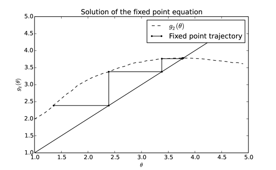
Figure 2: Fixed point iterations

The stopping rule is an equality since various values of $\theta$ produce only a finite number of sets $\mathcal{B}_{k}$ so that the only values produced by the iterations are the $\theta_{i}$. We can see the iteration procedure on Fig. 2 where we have shown the left-hand side in the form $y=\theta$ and the right-hand side $y=g_{2}(\theta)$. The solution is at the intersection of the two curves. We also show the points computed by the substitution algorithm.

The main advantage of this method is that there is no need to compute the $\theta_{i}$ and to sort them in advance. The problem with substitution methods is that it is difficult to guarantee convergence. But, in practice we have found that the fixed-point method always converged for all realistic values of the parameters.

We compare the cpu time of the four solution techniques in Table I. We have fixed $N=16$, $\hat{P}=5$, $c_{k}=1$ and generated the $\beta_{n,k}$ from a simple but realistic channel model. These values were obtained on a 2.5 GHz Intel Core i5 computer. We have computed the solution 100 times in each case to have a reasonably stable estimate. We can see that the fixed-point method is the fastest of all methods and the number of iterations does not change much with the problem size. The option is then between a technique with guaranteed convergence but somewhat slower than the other technique with no strict convergence guarantee. A compromise could be to use the fixed-point method and switch to the binary search technique if it has not converged within a small number of iterations, say 10.

M	Minos	Nonlinear		Binary		Fixed Point
	Cpu msec	Cpu msec	No iterations	Cpu msec	No iterations	Cpu msec	No iterations
2	23.3	19.0	20	1.5	0	2.0	3
4	71.8	43.8	21	12.6	6	4.2	3
8	292.	92.5	22	31.4	9	7.6	3

TABLE I: Computation load without rate constraints

IV Power Allocation with Rate Constraints

The problem of allocating power with rate constraints is solved in two steps. First, we try to allocate power without the rate constraints using one of the algorithms of section III since this is very fast. For the case where some of the RT users do not get their minimum rate, we propose in this section two algorithms that try to find a solution that is feasible both for the rate and power constraints, even though it may not be optimal. First we present an iterative algorithm that is guaranteed to produce a feasible solution with the rate constraints at their lower bounds. We then propose a non-iterative procedure that is faster but which is not guaranteed to find a feasible solution.

IV-A Feasible Solution at Bounds

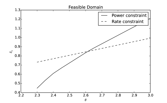
Figure 3: Domain for a single rate constraint

To simplify the discussion, consider first a problem with a single rate constraint, say for user 1. The boundaries of the two constraints (4–5) each define an implicit function $\delta_{1}(\theta)$. We can see an example of these boundaries on Fig. 3 for a small network with $K=2$, $N=8$, $P=2$ and a single real-time user. The set of feasible solution is the region above the rate constraint and below the power constraint.

A remarkable feature of this plot is that the boundary of the rate constraint seems to be linear. We already know that the boundary is piecewise linear but we now prove the following lemma.

Lemma 2.

The boundaries of the rate constraints are linear.

Proof.

If $\theta\approx 0$, all the $p_{n,k}\approx\infty$ and (5) will be a strict inequality. From the complementarity condition, we will then have $\delta_{k}=0$. This is consistent with the interpretation of $\theta$ as a penalty for the power constraint: If $\theta$ is small, there is no penalty for exceeding the power constraint so that there is a lot of power available. We can then choose large values of the $\overline{p}_{n,k}$ to increase the total rate so that the rate constraint will be an inequality.

As $\theta$ increases, there will be a point $\overline{\theta}_{k}$ where each rate $k$ constraint will become tight. This is given by

$$\overline{\theta}_{k}=\frac{c_{k}\sum_{n\in\mathcal{B}_{k}(\overline{\theta}_{k},0)}\beta_{n,k}}{\check{d}_{k}\log 2}.$$ (18)

At that point, we must increase $\delta_{k}\geq 0$ to stay on the boundary. For all values of $\theta\geq\overline{\theta}_{k}$, we choose a value of $\delta_{k}$ which is a linear function of $\theta$ with slope $m_{k}$

$$\delta_{k} =\left[m_{k}\theta-c_{k}\right]^{+}$$ (19)

$$m_{k} =\ln 2\left(2^{\check{d}_{k}}\prod_{n\in\mathcal{B}(\theta,\delta_{k})}\beta_{n,k}\right)^{\sigma(\theta,\delta_{k})^{-1}}.$$ (20)

With this choice of $\delta_{k}$, we know that the rate constraint in an equality over the whole range $\theta\geq\theta_{k}$ and from this, we see that

$$\overline{p}_{n,k} =\left[\frac{c_{k}+\delta_{k}}{\theta\log 2\beta_{n,k}}-1\right]^{+}$$

$$=\left[\frac{c_{k}+m_{k}\theta-c_{k}}{\theta\log 2\beta_{n,k}}-1\right]^{+}$$

$$=\left[\frac{m_{k}}{\log 2\beta_{n,k}}-1\right]^{+}$$

which is independent of $\theta$. In other words, once $\theta\geq\overline{\theta}_{k}$, the set $\mathcal{B}_{k}(\theta,\delta_{k})$ does not change and the rate constraint boundary is linear. ∎

We see from Fig. 3 that the point $(\theta^{(1)},0)$ where the power constraint boundary would meet the $\theta$ axis, is outside the feasible domain. The problem is to quickly find a point both above the rate boundary and below the power boundary and, if possible, a good point.

We make use of the linearity of the boundary to compute a feasible solution quickly by computing the intersection of the rate and power boundaries. First, we compute the slopes $m_{k}$ of the rate boundaries from (20) at the point $(\theta^{(1)},0)$. Given any value of $\theta$, we can then compute all the $\delta_{k}$’s from (19) and from this, the value of the total power $P(\theta)$ and total rate $R(\theta)$ from (10). We can see an example of these curves on Fig. 4.

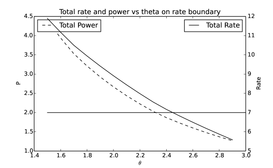
Figure 4: Rate and Power Curves vs $\theta$ on the Rate Boundaries

We compute the solution by solving $P(\theta)=\hat{P}$ by some numerical root-finding algorithm which is guaranteed to converge asymptotically. This is the best we can do if we impose the conditions that the rate constraints are met with equality since moving to the right on these boundaries means that the power constraint is not tight, which is a condition for an optimal solution.

IV-B Fast Heuristic

As we will see later, the time needed to compute a solution on the boundary may turn out to be too large for use in real time. Instead, we propose the following simple, non-iterative algorithm. The algorithm is based on the observation that a standard way to satisfy some constraint $k$ is to increase the corresponding multiplier $\delta_{k}$. From (10), we see that this will increase the $\overline{p}_{,nk}$ which will make the constraints more feasible. But this will also make the power constraint infeasible so that we need to increase $\theta$ as well. Let us define

$\theta^{(1)}$

the multiplier from the solution without rate constraints

$\overline{\theta}$

an upper bound on $\theta$ given by $\overline{\theta}=W\theta^{(1)}$ with $W>1$.

Starting from $\theta=\theta^{(1)}$, the heuristic basically moves a fixed amount in the direction of increasing $\theta$. At that point, it computes the solution on the rate boundaries and then tries to improve $\theta$ one more time as follows:

1. Compute the set of unsatisfied users $\mathcal{T}=\left\{k\mid r_{k}<\check{d}_{k}\right\}$.

2. Compute $\mathcal{B}_{k}(\overline{\theta},0)$

3. For users $k\not\in\mathcal{T}$, set $\delta_{k}^{(2)}=0$. For the other users, compute $\delta_{k}^{(2)}$ from (13) with $\theta=\overline{\theta}$ and $\mathcal{B}_{k}=\mathcal{B}_{k}(\overline{\theta},\delta_{k}^{(2)})$.

4. Compute a new $\theta^{(2)}$ from (14) with $\boldsymbol{\delta}=\boldsymbol{\delta}^{(2)}$ and $\mathcal{B}_{k}=\mathcal{B}(\overline{\theta},\delta_{k}^{(2)})$.

IV-C Improved Heuristic

The single iteration heuristic uses an arbitrary value $W$ for the step size which may not produce a very good solution. We can improve the results if we choose the parameter $W$ based on the difference between the required rate and the rate achieved by the maximum throughput PA. This increases the chance that the step will lead to a point to the right of the intersection of the two constraint curves. First we compute a different value of $W$ for each real-time user

$$W_{k}=2^{\epsilon(\check{d}_{k}-r_{k})}.$$ (21)

and then use the maximum $W_{k}$ among all RT users

$$W =\max_{k\in\mathcal{T}}W_{k}$$ (22)

$$\overline{\theta} =W\theta^{(1)}.$$ (23)

This way, we can increase the emphasis we want to put on meeting the rate constraints by increasing the value of $\epsilon$.

IV-D Infeasibility

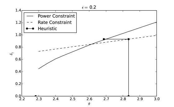
Figure 5: Fast Heuristic, Feasible Solution

We can see on Fig. 5 the path of the heuristic in the $(\theta,\delta)$ space with $\epsilon=0.2$. In this case, the final point is feasible since it lies above the rate boundary and lies on the power boundary. We say that the algorithm has succeeded. On the other hand, it is possible for the algorithm not to succeed for a variety of reasons. A practical approach could then be to try the fast heuristic first. If it fails, one could either try the zero-finding solution with a limited number of iterations or simply use the infeasible solution.

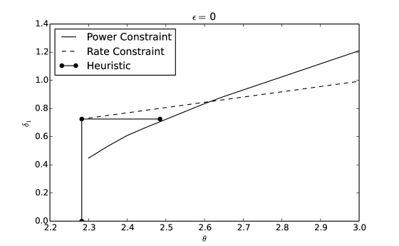
Figure 6: Fast Heuristic, Infeasible Solution

The first one is that we don’t know where the intersection of the two boundaries lie so that we don’t know how far to the right we must go to. Choosing a value of $\epsilon$ too small will not go far enough and the final point will not be feasible. This can be seen on Fig. 6 where we have chosen $\epsilon=0$. The point $(\overline{\theta},0)$ is to the right left of the intersection point of the two boundary curves so that moving to the right until we reach the power boundary still leaves us below the rate constraint. In this case, the algorithm has failed.

There is another, more subtle reason, why the algorithm may fail. Consider the final point of figure 5. We can see that the point is slightly to the left of the power boundary. The reason is that we compute $\theta^{(2)}$ using $\mathcal{B}_{k}(\overline{\theta},\delta_{k}^{(2)})$ which is not the same as $\mathcal{B}_{k}(\theta^{(2)},\delta_{k}^{(2)})$, hence the small error.

Another potential problem is that by increasing $\theta$ from $\theta^{(1)}$, the heuristic algorithm reduces the power of the users that are not in $\mathcal{T}$. If some of these are RT users and have a rate close to $\check{d}_{k}$, they may become unfeasible. A simple solution is to add these users to $\mathcal{T}$ by increasing their $\check{d}_{k}$ and run the fast heuristic again.

We can see that the algorithm produces a feasible point as follows. We assume that users close to the unfeasibility boundary are all included in set $\mathcal{T}$ by increasing their $\check{d}_{k}$.

Lemma 3.

When successful, the fast algorithm produces a feasible point to problem (3–5).

Proof.

By construction, the final point lies on the power boundary. It also lies above the rate boundary for the following reason. The point $(\overline{\theta},\delta_{k}^{(2)})$ lies on the rate boundary by construction. Given that the slope of the rate boundary is positive, all the poinst $(\theta,\delta_{k}^{(2)})$ with $\theta<\overline{\theta}$ will also lie above the boundary. ∎

Note also that this method can be used with an arbitrary method for computing the unconstrained power allocation, such as [5, 15, 6], as long as we get the value of $\theta^{(1)}$ from the solution.

V Numerical Evaluation

In this section, we compare the three different methods to solve problem (3–7): An exact solution by a nonlinear solver [20], the boundary solution of IV-A and the fast heuristic of IV-C. We look at their accuracy and the cpu time needed to compute a solution. The nonlinear equations were solved by the netlib function bisect through the Scipy Python interface. All results were obtained on an Intel Core i5 cpu running at 2.5 GHz.

V-A Generating Test Cases

Each test case is defined first by the set $(K,N,M,P)$. We use a Rayleigh fading model to generate the user channels such that each component of the channel vectors $h_{k,n}$ are i.i.d. random variables distributed as $\mathcal{CN}(0,1)$. We also assume independent fading between users, antennas and subcarriers. We assign the subchannels with a variant of the semiorthogonal user selection (SUS) heuristic [2] and then compute the $\beta_{n,k}$ from this. After this, we select the number of real-time users $R$. The set of values we have used is shown in Table II.

Number	$K$	$N$	$M$	$\hat{P}$	$R$
II	20	25	2	5	3
II	20	25	2	5	10
II	80	25	2	5	0
II	80	25	2	5	10
II	80	25	2	5	20
II	80	25	2	5	30
II	80	25	2	5	40
II	80	25	2	5	50
II	80	25	2	5	60

TABLE II: Parameters for Test Cases

The next step is to generate the rate bounds in such a way that the problems are known to be feasible. Also, we would like to control the “difficulty” of the problem to see how much this impacts on the accuracy and cpu time. First, we maximize the total rate of real-time users by solving problem (3–4) over the $p_{n,k},\,k\in\mathcal{D}$ only and without the rate constraints. Call this problem $P_{0}$ and $R_{0}$ the total rate of the real-time users. We then know there is enough power to give the real-time users the rates $r_{k}^{(0)}$ produced by the unconstrained solution.

This means that any problem $P_{1}$ with rate constraints $\check{d}_{k}=r_{k}^{(0)}$ has a feasible solution with only the real-time users having a positive rate and with the rate constraints at their bounds. If this were not the case, there would be some spare power that could be used to construct a solution to $P_{0}$ with a total rate $R_{1}>R_{0}$ which contradicts the fact that $R_{0}$ is the optimal value for $P_{0}$.

We also know that any problem with rate constraints $\check{d}_{k}=sr_{k}^{(0)}$ is feasible if $0\leq s\leq 1$. Furthermore, the value of $s$ is a rough measure of the “tightness” of the constrained data set. The problem is unconstrained when $s=0$ and is tightly constrained when $s=1$ where only the real-time users can get some power. The scale $s$ will be the primary parameter used to display results.

V-B Effect of $\epsilon$

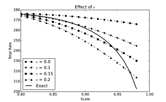
Figure 7: Effect of $\epsilon$ on Heuristic

First we examine the effect of $\epsilon$ on the accuracy of the fast heuristic for problem II. This is show on Fig. 7 where we plot the objective value computed by the heuristic for different values of $\epsilon$ and also the optimal value computed by the nonlinear solver as a function of the scale parameter. For each curve corresponding to the heuristic, we can define a range of values of $s$ where the heuristic value is below the optimal rate and one where it is above. In this latter case, this is an indication that the solution computed by the heuristic is not feasible. The curves show that there is a clear tradeoff between the accuracy of the solution and the range of problems where the solution is feasible. For small values of $\epsilon$, the range of problems where the heuristic can produce a feasible solution is quite small but the solutions are quite accurate. This is opposite to the curves with large $\epsilon$ where the algorithm can compute feasible solutions over a larger range of problems but where the objective function solution is not as good.

V-C Solution Accuracy

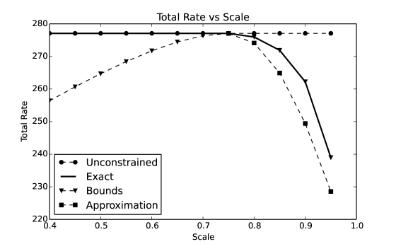
Figure 8: Accuracy of Heuristics, Small Network, Few Real-Time Users

Next we show the accuracy of the two heuristics by comparing the total rate they produce with the exact value as a function of the scale parameter. In all cases, we choose $\epsilon=0.2$. The first case is for problem II shown on Fig. 8. Here, it turns out that all the rate constraints are at their bound in the optimal solution. This is not unexpected if we have a small number of real-time users: There is a good chance that other users may have a better channel so that once the constraints is satisfied, it is more useful to allocate the power to these non real-time users since they will get a better rate.

Figure 9: Accuracy of Heuristics, 10 Real-time Users

A similar result is shown for problem II on Fig. 9. This has the same parameters as problem II but this time with 10 real-time users. Here too we see that the rate constraints are at their bound in the optimal solution. The approximate heuristic does a rather poor job of finding a feasible solution for the value of $\epsilon=0.2$ that we have chosen.

The rate bounds in the example of Fig. 9 are computed from the problem data and in a sense they “fit” the values of $\beta$. In practice, the rate requirement of real-time users would be determined by the application independently of the channel conditions. To see the accuracy of the solution techniques on these cases, we have produced the bounds somewhat differently. First, we assume that there is a small number of applications, three in the present case, with different rate bounds $\check{d}_{k}^{(0)}$ in the ratio 1:4:16. For example, this could correspond to voice, fast data transfer and video. We then compute the largest scaling factor $\gamma$ such that the problem is feasible with bounds $\check{d}_{k}=\gamma\check{d}_{k}^{(0)}$. We can then control how difficult the problem is by selecting some scale between 0 and 1 to scale the bounds $\check{d}_{k}$ as above.

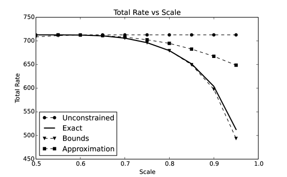
Figure 10: Accuracy for Fixed Rate Bounds, Problem II

We show on Fig. 10 the accuracy of the algorithm for problem II with the given rate bounds. We can see that the solution on the boundary is still very close to the optimal solution and the fast heuristic produces an infeasible solution. Note however that this case has only 10 real-time users out of 80.

Figure 11: Accuracy for Fixed Rate Bounds, Problem II

The situation is quite different if we have 60 real-time users as in problem II. These users are divided into 3 groups of 20 and all users in a group have the same requirement in the order 1:4:16. We can see from Fig. 11 that the solution on the rate bounds is much lower than the optimal value for quite a large range of scales and the fast heuristic again produces infeasible solutions.

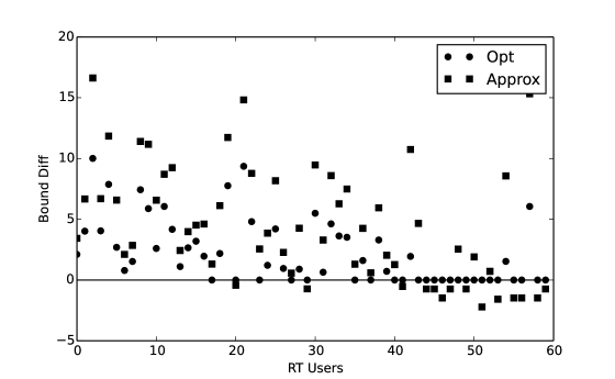
Figure 12: Difference with Rate Bounds

We can get a better understanding of these results from Fig. 12 where we plot, for each real-time user and scale 1, the difference $r_{k}-\check{d}_{k}$ for the optimal solution and the approximation. As expected, in the optimal solution, all users are above zero, since the solution has to be feasible. More important is the fact that for the first two groups, the ones with the lower bounds, most users actually get more that their minimum rate. This explains the poor behavior of the bounds algorithms which computes an optimal solution on the boundary. Also interesting is the approximate solution for the third group, the one with high rate. We see that the approximate solution is infeasible but that the amount of infeasibility is rather small. Note that this is a relatively hard problem in the sense that the problem is barely feasible in the first place. Given that the solution produced by the bounds algorithm is not very good, a reasonable solution would then be to use the approximation and give some real-time users slightly less than what they require. This may be acceptable considering that the channel conditions will change at the next time frame and that it may then be possible to give these users the rate that they require.

V-D CPU Time

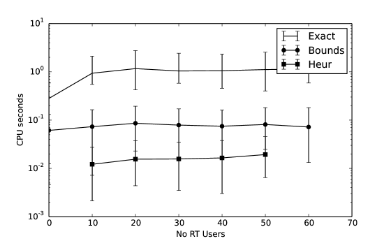
Figure 13: CPU Time vs No of RT Users

We present in Fig. 13 the cpu time required by the nonlinear solver, labelled exact, the algorithm on the rate boundary, labelled bounds and the heuristic, labelled heur. The values of the computation times are plotted as a function of the number of real-time users $R$ for problems II–II. For each value of $R$, we have measured the average, maximum and minimum cpu time required for solving the problem over the whole range of values of $s$. The maximum and minimum values are presented as error bars. We can see that there is about one order of magnitude between each algorithm. The heuristic takes in the order of 10 ms while the bounds algorithm, about 10 times as much.

VI Conclusions

We have looked at the problem of allocating power to a given set of users in a ZF OFDMA-SDMA system with some real-time users with minimum transmission rate requirements. The approach is to solve the problem in two steps. First, we solve without taking into account the rate constraints. For this, we provide two fast algorithms. The first one is based on the solution of the first-order optimality condition via a zero-finding algorithm. We use the structure of the problem to perform a search over a finite number of intervals for the one containing the solution. From this, we get the exact value of the solution so that the algorithm is guaranteed to find a solution in $O(\log_{2}NK)$ steps.

The second algorithm is based on re-writing the optimality conditions as a fixed-point equation which we can solve by repeated substitution. This is faster than the zero-finding method but there is no guarantee that it will converge. We have found that in practice, convergence always occurs in a small number of iterations for all the cases we have tested.

If the solution is feasible, this is the optimal solution for the constrained problem as well. If some real-time users do not get their minimum rate, we propose two approximate techniques to compute a feasible, or nearly feasible solution by adjusting the dual multipliers. First, we show that the boundary of the rate constraints is linear in the $(\theta,\delta)$ plane. We then use this to propose an algorithm to compute a solution on the rate boundaries. This is based on finding a zero of the first-order equations for the value of $\theta$ only, since we can use the linearity of the rate boundary to keep the solution feasible.

The second approximation is not iterative and is a one-step adjustment of the multipliers. It is parameterized in such a way that we can emphasize either feasibility, at the cost of having a somewhat less than optimal value for the rate, or efficiency, where the rate is relatively large but some real-time users get somewhat less than their required rate.

Finally, we present some results for the cpu time needed by three algorithms: the exact solution by a nonlinear solver, the bounds algorithm and the approximation. We find that there is roughly one order of magnitude between each, where the bounds algorithm is an order of magnitude faster than the exact solution, and the fast heuristic is an additional order of magnitude faster.

References

- [1] A. Wiesel, Y. Eldar, and S. Shamai, “Optimal generalized inverses for zero forcing precoding,” in Proc. of 41st Annual Conf. on Information Sciences and Systems, 2007.
- [2] T. Yoo and A. Goldsmith, “On the optimality of multiantenna broadcast scheduling using zero-forcing beamforming,” IEEE Journal on Selected Areas in Communications, vol. 24, no. 3, pp. 528–541, Mar. 2006.
- [3] X. Wang and G. Giannakis, “Resource allocation for wireless multiuser OFDM networks,” IEEE Trans. in Information Theory, vol. 57, no. 7, pp. 4359–4372, 2011.
- [4] D. Perez-Palomar and M. Lagunas, “Joint transmit-receive space-time equalization in spatially correlated MIMO channels: a beamforming approach,” IEEE Journal on Selected Areas in Communications, vol. 21, no. 5, pp. 730–743, 2003.
- [5] X. Ling, B. Wu, P.-H. Ho, F. Luo, and L. Pan, “Fast water-filling for agile power allocation in multi-channel wireless communications,” IEEE Communications Letters, vol. 16, no. 8, pp. 1212–1215, 2012.
- [6] J. Jang and a. Y. L. K. B. Lee, “Transmit power and bit allocations for OFDM systems in a fading channel,” in Proc. IEEE Global Communication Conference, Globecom, vol. 2, 2003, pp. 858–862.
- [7] G. Dimic and N. Sidiropoulos, “On downlink beamforming with greedy user selection: performance analysis and a simple new algorithm,” IEEE Transactions on Signal Processing, vol. 53, no. 10, pp. 3857–3868, 2005.
- [8] D. Perea-Vega, J. Frigon, and A. Girard, “Near-optimal and efficient heuristic algorithms for resource allocation in MISO-OFDM systems,” in IEEE International Conference on Communications ICC, May 2010, pp. 1–6.
- [9] V. Papoutsis and S. Kotsopoulos, “Resource Allocation Algorithm for MISO-OFDMA Systems with QoS Provisioning,” in Proc. ICWMC, The Seventh International Conference on Wireless and Mobile Communications, Jun. 2011.
- [10] D. Perea-Vega, J. Frigon, and A. Girard, “Efficient Heuristic for Resource Allocation in Zero-forcing OFDMA-SDMA Systems with Minimum Rate Constraints,” in — In preparation, available on-line at …, 2013.
- [11] D. Bertsekas, Convex Analysis and Optimization. Athena Scientific – Belmont, MA, 2003.
- [12] 3GPP, “3GPP: Evolved Universal Terrestrial Radio Access (E-UTRA); Base Station radio transmission and reception; Further advancements for E-UTRA physical layer aspects,” 3GPP TR V10.5, Tech. Spec.n Group Radio Access Network.
- [13] J. Jang and K. Lee, “Transmit power adaptation for multiuser OFDM systems,” IEEE Journal on selected areas in Communications, vol. 21, no. 2, pp. 171–178, Feb. 2003.
- [14] M. Anas, K. Kim, S. Shin, and K. Kim, “QoS Aware power allocation for combined guaranteed performance and best effort users in OFDMA systems,” in Proc. of International Symposium on Intelligent Signal Processing and Communication Systems, 2004, pp. 477–481.
- [15] W. Yu, W. Rhee, S. Boyd, and J. Cioffi, “Iterative water-filling for gaussian vector multiple-access channels,” IEEE Transactions on Information Theory, vol. 50, no. 1, pp. 145–152, 2004.
- [16] S. Zhu, G. Lv, and H. Hui, “A low complexity heuristic adaptive resource llocation algorithm for multiuser OFDM under rate constraints,” in Communications and Networking in China, 2009. ChinaCOM 2009. Fourth International Conference on, Aug 2009, pp. 1–4.
- [17] D. Kivanc, G. Li, and H. Liu, “Computationally efficient bandwidth allocation and power control for OFDMA,” Wireless Communications, IEEE Transactions on, vol. 2, no. 6, pp. 1150–1158, Nov 2003.
- [18] L. V. S. Boyd, Convex Optimization. Cambridge University Press, 2004.
- [19] M. Tao, Y.-C. Liang, and F. Zhang, “Resource allocation for delay differentiated traffic in multiuser OFDM systems,” IEEE Trans. on Wireless Communications, vol. 7, no. 6, pp. 2190–2201, 2008.
- [20] B. A. Murtaugh and M. A. Saunders, “MINOS 5.4 users guide,” Department of Operations Research, Stanford University, Stanford, CA 94305 USA, Tech. Rep. SOL 83-20R, Dec. 1993.