Darboux transformation of the second-type derivative nonlinear Schrödinger equation

Abstract.

The second-type derivative nonlinear Schrödinger (DNLSII) equation was introduced as an integrable model in 1979. Very recently, the DNLSII equation has been shown by an experiment to be a model of the evolution of optical pulses involving self-steepening without concomitant self-phase-modulation. In this paper the $n$-fold Darboux transformation (DT) $T_{n}$ of the coupled DNLSII equations is constructed in terms of determinants. Comparing with the usual DT of the soliton equations, this kind of DT is unusual because $T_{n}$ includes complicated integrals of seed solutions in the process of iteration. By a tedious analysis, these integrals are eliminated in $T_{n}$ except the integral of the seed solution. Moreover, this $T_{n}$ is reduced to the DT of the DNLSII equation under a reduction condition. As applications of $T_{n}$, the explicit expressions of soliton, rational soliton, breather, rogue wave and multi-rogue wave solutions for the DNLSII equation are displayed.

Keywords: The second-type derivative nonlinear Schrödinger equation, Darboux transformation, breather solution, rogue wave solution, self-steepening.

MSC(2010) numbers: 35C08, 35C11, 35Q55, 37K40, 78A60

1. Introduction

In 1979, Chen-Lee-Liu (CLL) linearized the nonlinear Hamiltonian systems and identified it with the time part of the Lax equation in order to test the integrability of nonlinear Hamiltonian systems by inverse scattering method [1]. Moreover, several integrable equations and non-integrable equations were introduced. Among them, there is a derivative-type nonlinear equation

$${\rm i}q_{t}+q_{xx}+{\rm i}|q|^{2}q_{x}=0,$$ (1)

which is integrable and is usually called Chen-Lee-Liu(CLL) equation or the second-type derivative nonlinear Schrödinger equation (DNLSII). Via the Hirota method, the explicit formula of $n$-soliton solution of the DNLSII equation was obtained [2, 3]. The Lax pair for the DNLSII equation was generalized into matrix-type and new integrable coupled derivative nonlinear Schrödinger equations were obtained [4]. The Cauchy problem of the semi-classical DNLSII equation was studied [5] under a rapidly oscillating initial profile. Except the DNLSII equation, there exists another type of DNLS equation, i.e. the first type derivative nonlinear Schrödinger equation (DNLSI) [6]

$${\rm i}\tilde{q}_{t}+\tilde{q}_{xx}+{\rm i}(|\tilde{q}|^{2}\tilde{q})_{x}=0,$$ (2)

which is connected with the DNLSII equation by a simple gauge transformation [8, 7] of form $\tilde{q}=q\exp\left(-\frac{\rm i}{2}\int^{x}|q|^{2}\mathrm{d}x\right)$, with a trivial but very important observation $|q|^{2}=|\tilde{q}|^{2}$, the inverse gauge transformation is given by

$$q=\tilde{q}\exp\left(\frac{\rm i}{2}\int^{x}|\tilde{q}|^{2}\mathrm{d}x\right).$$ (3)

By comparing with the intensive investigations on the DNLSI equation from the point of views of mathematics and physics, e.g. see [9, 10, 11, 12, 13, 14, 15, 16] and references therein, the DNLSII equation has received little attention as mentioned above in the past decades, to the best of our knowledge. Perhaps, there are two reasons for the opposite fate of the two types of the DNLS equation.

• The lack of physical relevance of the DNLSII equation for a very long time. In contrast to the direct applications in plasmas [10, 11, 12, 16], water wave [13] and nonlinear optics [14, 15] of the DNLSI equation, the DNLSII equation is only known to model the propagation of the self-steepening optical pulses without self-phase modulation [17] in 2007.
  

• The doubt of necessity of the study of explicit solutions $q$ for the DNLSII equation. This well-known doubt is originated from that the modulus of $q$, a solution of the DNLSII equation, can be calculated from a known solution $\tilde{q}$ of the DNLSI equation through the gauge transformation eq.(3). The latter has been solved exactly by various methods such as the inverse scattering transformation, bilinear method and Darboux transformation (DT) [6, 18, 19, 20, 21, 22, 3, 23, 24].

However, the above two reasons are fading fast at the present time, and then from now on the DNLSII equation deserves further studies. Physically, the self-steepening of light pulses, originating from its propagation in a medium with an intensity dependent index of refraction, was first introduced in [25], and later was observed in optical pulses with possible shock formation [26]. The isolated self-steepening is less common in nature and is often studied in conjunction with self-phase-modulation [14, 15]. In other words, it is very difficult to observe self-steepening alone although a controllable self-steepening has been suggested in theory and demonstrated in experiment in 2006 through the wave vector mismatch [27]. Soon after, at 2007, J. Moses, B. A. Malomed and F. W. Wise [17] have reported an experimental manifestation in optical pulses propagation involving self-steepening without self-phase-modulation. This experiment provides the first physical realization of the DNLSII equation, and further shows that the DNLSII equation, like the nonlinear Schrödinger(NLS) equation and DNLSI equation, is also a real and important physical model. Although the gauge transformation (3) gives the expression of $q$ with an integral from a known solution $\tilde{q}$, this integral makes the process of getting multi-soliton solutions very difficult. Therefore, it is an interesting problem to seek new solutions, e.g. breather and rogue wave, of the DNLSII equation which are not generated by gauge transformation (3) from corresponding known solutions of the DNLSI equation.

The rogue waves, appearing from nowhere and disappearing without a trace [28], have drawn much attention both from theoretical predictions and experimental observations. Theoretically, a possible generating mechanisms for the rogue waves of the NLS equation is introduced as follows [29]: the progressive fusion and fission of $n$ degenerate breathers associated with a critical eigenvalue $\lambda_{0}$ creates an order-$n$ rogue wave. The value $\lambda_{0}$ is a zero point of an eigenfunction of the Lax pair of the NLS equation and it corresponds to the limit that the period of the breather tends to infinity. After the debate for several decades, the rogue wave has been observed experimentally very recently in nonlinear fiber optics, in water-wave tanks, and in plasmas [30, 31, 32, 33].

In addition to above important experiment works, the analytical and simple form of the rogue waves for the integrable partial differential equations(PDEs) is one of central topics in recent years. Up to now the DT becomes one of the cornerstones in the approach to construct analytical forms of the rogue waves. More generally, the Darboux transformation, as a known world-wide method, provides a systematic way to study the explicit solutions of the integrable systems after the pioneering works in 1979 [34, 35, 36, 37], which had extended a simple lemma by Darboux(1882) dealing with 1–dimensional scalar Schrödinger equation to the hierarchies of linear and nonlinear PDE’s and their non-commutative, differential–difference and difference–difference (i.e. lattice) version. Since long time (from 1983 and until 2010) the study of the connections between the analytical rogue waves and integrable PDEs was limited by the very special solutions including the genuine Peregrine breather discovered by Peregrine himself in 1983 [38] and its two next higher analogues: $P_{2}$ breather and $P_{3}$ breather discovered by Akhmediev, Eleonsky and Kulagin in 1985 [39] and $P_{3}$ breathers found by Akhmediev and his coworkers in 2009 [40]. These solutions were describing the simplest rogue events in the fibers optics and hydrodynamics. At the same period Ankiewicz, Akhmediev and Clarkson(2010) produced a conjecture about the existence of the hierarchy of similar isolated solutions labeled by the integer $n$ reaching at a single point of space time the maximum of its absolute value equal $2n+1$ provided that the asymptotic magnitude of the solution equals 1 [41]. In 2011, they succeeded to partially justify this conjecture only partially, by calculating explicitly the initial data for $P_{4}$ and $P_{5}$ by use of the DT method [42], but not the complete solutions. Similar solutions were found at the same period for many other physical systems relevant to various physical applications by different authors [43, 44, 45, 46].

In 2010, Matveev and his coauthors have significantly developed the technique of obtaining multi-rogue wave (MRW) solutions and presented explicit forms for these higher order structures via explicit Wronskian formulas at the first time[47], and then given a series papers on the properties and compact forms of MRW [48, 49, 50, 51]. It was conjectured in [48](see page 30) that, for an order-$n$ rogue wave under the fundamental pattern of the NLS, the number of these maxima in space-time is $n(n+1)-1$ with one “super peak” of the height $2n+1$ surrounded by $n(n+1)-2$ gradually decreasing peaks in two sides. They further have conjectured that there exist other pattern of an order-$n$ rogue wave possessing $n(n+1)/2$ uniform peaks [48, 49, 50]. In [52] it was also shown that how to construct the initial data for KP–I equation in order to produce the extremal rogue wave events caused by the collision of the simple rogue waves. The attached movies gave an understanding of various scenario of collisions of the simple rogue waves in the KP–I model, leading in particular to short–living $2+1$ dimensional extremal rogue waves on a shallow water. Later, many authors studied different models using Hirota method, Darboux transformation approach, and thus the whole research of analytical theory for rogue wave is growing very rapidly [44, 45, 46, 53, 54].

These existed results inspire us to seek breather and rogue wave solutions of the DNLSII equation without using the DNLSI equation. We can further show the independent value of this physical model and stimulate new way to observe the rogue waves by using self-steepening effect in optical system. Meanwhile, a rogue wave solution of the DNLSII equation may be used conveniently to observe the self-steepening effect alone because of its high-amplitude and localized property in $(x,t)$ plane. To this end, we are going to construct the DT and its determinant representation of the DNLSII equation, and then use it to generate the intended solutions, i.e. soliton, breather and rogue wave. Although there are several well-known results of DT for the NLS equation [57, 58, 59, 60, 55, 56, 61] and two other types of the DNLS equation [23, 62], the DT of the DNLSII equation is non-trivial because it includes an complicated integral of seed solution, as we shall show later. This kind of DT for soliton equations has not been reported so far as the authors know.

The present paper is organized as follows. In section 2, we give a detailed derivation of the determinant representation $T_{n}$ of the $n$-fold DT for the coupled DNLSII equations. Particularly, the first order DT—$T_{1}$ depends on an integral of the seed solution, which is different from the usual DT. Through a cumbersome analysis, we eliminate this kind of integral depending on higher order potentials and simplify the expression of the $T_{n}$. The reduction of the $T_{n}$ to the DNLSII equation is also obtained in this section. In section 3, the soliton, rational soliton, breather, rogue wave and multi-rogue wave solutions are given by applying the multi-fold DT of the DNLSII equation. The relationship between solutions of the DNLSII equation and the DNLSI equation is discussed. Finally, conclusions and discussions are given in section 4.

2. Darboux transformation

In this section, we will construct the DT of the coupled DNLSII equations

$${\rm i}q_{t}+q_{xx}+{\rm i}qrq_{x}=0,$$ (4a)

$${\rm i}r_{t}-r_{xx}+{\rm i}rqr_{x}=0.$$ (4b)

This system is the compatibility condition of the following Lax pair [7]:

$$\left\{\begin{aligned} \Phi_{x}&=U\Phi=({\rm-i}\lambda^{2}+\frac{\rm i}{4}qr)J\Phi+\lambda Q\Phi,\\ \Phi_{t}&=V\Phi=(-2{\rm i}\lambda^{4}+{\rm i}qr\lambda^{2}+\frac{1}{4}(qr_{x}-rq_{x})-\frac{\rm i}{8}q^{2}r^{2})J\Phi+2\lambda^{3}Q\Phi+\lambda W\Phi,\end{aligned}\right.$$ (5)

with

$$\Phi(x,t,\lambda)=\left(\begin{matrix}f(x,t,\lambda)\\ g(x,t,\lambda)\end{matrix}\right),\quad J=\left(\begin{matrix}1&0\\ 0&-1\end{matrix}\right),\quad Q=\left(\begin{matrix}0&q\\ -r&0\end{matrix}\right),\quad W=\left(\begin{matrix}0&{\rm i}q_{x}-\frac{1}{2}q^{2}r\\ {\rm i}r_{x}+\frac{1}{2}r^{2}q&0\end{matrix}\right).$$

Under a reduction condition $r=q^{*}$, two equations (4) are reduced to the DNLSII equation.

2.1 The first order Darboux transformation

In general, we suppose

$$T(\lambda)=\left(\begin{array}[]{cc}a_{1}&b_{1}\\ c_{1}&d_{1}\end{array}\right)\lambda+\left(\begin{array}[]{cc}a_{0}&b_{0}\\ c_{0}&d_{0}\end{array}\right)$$ (6)

is the first order DT of the coupled DNLSII equations, i.e. there exist $U^{[1]}$ and $V^{[1]}$ possessing the same form as $U$ and $V$ with $q$ and $r$ replaced by the new potentials $q^{[1]}$ and $r^{[1]}$, such that $\Phi^{[1]}=T\Phi$ satisfies

$$\Phi^{[1]}_{x}=U^{[1]}\Phi^{[1]},\quad\Phi^{[1]}_{t}=V^{[1]}\Phi^{[1]}.$$ (7)

As given in [55, 56], $T(\lambda)$ must satisfy following conditions

$$T_{x}+TU=U^{[1]}T,\quad T_{t}+TV=V^{[1]}T$$ (8)

according to eq.(7). Here $a_{0},b_{0},c_{0},d_{0},a_{1},b_{1},c_{1},d_{1}$ are the functions of $x$ and $t$ need to be determined. Comparing the coefficients of $\lambda^{j},(j=3,2,1,0)$ in the $x$-part of (8), we obtain

$$\lambda^{3}$$:

$$b_{1}=0,\quad c_{1}=0,$$ (9a)

$$\lambda^{2}$$:

$$a_{1}q+2{\rm i}b_{0}-q^{[1]}d_{1}=0,\quad r^{[1]}a_{1}-2{\rm i}c_{0}-d_{1}r=0,$$ (9b)

$$\lambda^{1}$$:

$$\frac{1}{4}{\rm i}a_{1}qr+a_{1x}-\frac{1}{4}{\rm i}a_{1}q^{[1]}r^{[1]}-b_{0}r-q^{[1]}c_{0} =0,\quad a_{0}q-q^{[1]}d_{0}=0,$$ (9c)

$$\frac{1}{4}{\rm i}d_{1}q^{[1]}r^{[1]}+d_{1x}-\frac{1}{4}{\rm i}d_{1}qr+c_{0}q+r^{[1]}b_{0} =0,\quad r^{[1]}a_{0}-d_{0}r=0,$$

$$\lambda^{0}$$:

$$-\frac{1}{4}{\rm i}a_{0}q^{[1]}r^{[1]}+a_{0x}+\frac{1}{4}{\rm i}a_{0}qr =0,\quad-\frac{1}{4}{\rm i}b_{0}qr+b_{0x}-\frac{1}{4}{\rm i}b_{0}q^{[1]}r^{[1]}=0,$$ (9d)

$$\frac{1}{4}{\rm i}c_{0}qr+c_{0x}+\frac{1}{4}{\rm i}c_{0}q^{[1]}r^{[1]} =0,\quad-\frac{1}{4}{\rm i}d_{0}qr+d_{0x}+\frac{1}{4}{\rm i}d_{0}q^{[1]}r^{[1]}=0.$$

Similarly, the $t$-part of (8) leads to

$$\lambda^{4}:$$

$$-2q^{[1]}d_{1}+2a_{1}q+4{\rm i}b_{0}=0,\quad-4{\rm i}c_{0}-2d_{1}r+2r^{[1]}a_{1}=0,$$ (10a)

$$\lambda^{3}:$$

$$-q^{[1]}r^{[1]}a_{1}{\rm i}-2b_{0}r-2q^{[1]}c_{0}+a_{1}qr{\rm i} =0, \quad 2a_{0}q-2q^{[1]}d_{0}=0,$$ (10b)

$$2r^{[1]}b_{0}+q^{[1]}r^{[1]}d_{1}{\rm i}+2c_{0}q-d_{1}qr{\rm i} =0, \quad-2d_{0}r+2r^{[1]}a_{0}=0,$$

$$\lambda^{2}$$:

$$a_{0}qr{\rm i}-q^{[1]}r^{[1]}a_{0}{\rm i}=0,\qquad-d_{0}qr{\rm i}+q^{[1]}r^{[1]}d_{0}{\rm i} =0,$$ (10c)

$$-q^{[1]}r^{[1]}b_{0}{\rm i}-\frac{1}{2}a_{1}q^{2}r-q^{[1]}_{x}d_{1}{\rm i}+\frac{1}{2}{q^{[1]}}^{2}r^{[1]}d_{1}-b_{0}qr{\rm i}+a_{1}q_{x}{\rm i} =0,$$

$$-{\rm i}r^{[1]}_{x}a_{1}-\frac{1}{2}q^{[1]}{r^{[1]}}^{2}a_{1}+\frac{1}{2}d_{1}qr^{2}+q^{[1]}r^{[1]}c_{0}{\rm i}+c_{0}qr{\rm i}+{\rm i}d_{1}r_{x} =0,$$

$$\lambda^{1}$$:

$$\frac{1}{2}{q^{[1]}}^{2}r^{[1]}d_{0}-q^{[1]}_{x}d_{0}{\rm i}-\frac{1}{2}a_{0}q^{2}r+a_{0}q_{x}{\rm i}=0,\quad-\frac{1}{2}q^{[1]}{r^{[1]}}^{2}a_{0}-r^{[1]}_{x}a_{0}{\rm i}+d_{0}r_{x}{\rm i}+\frac{1}{2}d_{0}qr^{2}=0,$$ (10d)

$$\frac{1}{2}c_{0}{q^{[1]}}^{2}r^{[1]}-\frac{1}{4}q^{[1]}r^{[1]}_{x}a_{1}+\frac{1}{4}a_{1}qr_{x}+\frac{1}{2}b_{0}qr^{2}+\frac{1}{4}r^{[1]}q^{[1]}_{x}a_{1}-\frac{1}{8}{\rm i}a_{1}q^{2}r^{2}-c_{0}q^{[1]}_{x}{\rm i}-\frac{1}{4}a_{1}rq_{x}$$

$$+b_{0}r_{x}{\rm i}+\frac{1}{8}{\rm i}{q^{[1]}}^{2}{r^{[1]}}^{2}a_{1}+a_{1t}=0,$$

$$\frac{1}{4}d_{1}rq_{x}+\frac{1}{4}q^{[1]}r^{[1]}_{x}d_{1}+c_{0}q_{x}{\rm i}-\frac{1}{4}d_{1}qr_{x}+\frac{1}{8}{\rm i}d_{1}q^{2}r^{2}+d_{1t}-\frac{1}{2}c_{0}q^{2}r-b_{0}r^{[1]}_{x}{\rm i}-\frac{1}{8}{\rm i}{q^{[1]}}^{2}{r^{[1]}}^{2}d_{1}$$

$$-\frac{1}{4}r^{[1]}q^{[1]}_{x}d_{1}-\frac{1}{2}b_{0}q^{[1]}{r^{[1]}}^{2}=0,$$

$$\lambda^{0}:$$

$$\frac{1}{4}r^{[1]}q_{x}a_{0}+a_{0t}+\frac{1}{4}a_{0}qr_{x}-\frac{1}{4}q^{[1]}r_{x}a_{0}+\frac{1}{8}{\rm i}{q^{[1]}}^{2}{r^{[1]}}^{2}a_{0}-\frac{1}{8}{\rm i}a_{0}q^{2}r^{2}-\frac{1}{4}a_{0}rq_{x}=0,$$ (10e)

$$b_{0t}+\frac{1}{4}b_{0}r^{[1]}q_{x}+\frac{1}{8}{\rm i}b_{0}{q^{[1]}}^{2}{r^{[1]}}^{2}+\frac{1}{8}{\rm i}b_{0}q^{2}r^{2}-\frac{1}{4}b_{0}qr_{x}+\frac{1}{4}b_{0}rq_{x}-\frac{1}{4}b_{0}q^{[1]}r_{x}=0,$$

$$c_{0t}-\frac{1}{8}{\rm i}c_{0}q^{2}r^{2}+\frac{1}{4}c_{0}q^{[1]}r_{x}+\frac{1}{4}c_{0}qr_{x}-\frac{1}{4}c_{0}rq_{x}-\frac{1}{4}c_{0}r^{[1]}q_{x}-\frac{1}{8}{\rm i}c_{0}{q^{[1]}}^{2}{r^{[1]}}^{2}=0,$$

$$\frac{1}{8}{\rm i}d_{0}q^{2}r^{2}-\frac{1}{4}d_{0}qr_{x}+\frac{1}{4}d_{0}rq_{x}+\frac{1}{4}q^{[1]}r_{x}d_{0}-\frac{1}{8}{\rm i}{q^{[1]}}^{2}{r^{[1]}}^{2}d_{0}-\frac{1}{4}r^{[1]}q^{[1]}_{x}d_{0}+d_{0t}=0.$$

From (9c), we have $a_{0}=d_{0}=0$ in order to get non-trivial transformation. Therefore, suppose the first order DT is of form form of

$$T_{1}(\lambda;\lambda_{1})=\left(\begin{array}[]{cc}a_{1}&0\\ 0&d_{1}\end{array}\right)\lambda+\left(\begin{array}[]{cc}0&b_{0}\\ c_{0}&0\end{array}\right).$$ (11)

The reason of the appearance of $\lambda_{1}$ in eq.(11) is that we shall use the eigenfunction associated with $\lambda_{1}$ to parameterize the coefficients of $T_{1}$ with the help of eqs.(9a) to (10e).

It is easy to get $(a_{1}d_{1})_{x}=0,\,(a_{1}d_{1})_{t}=0,\,(b_{0}c_{0})_{x}=0,\mbox{ and }(b_{0}c_{0})_{t}=0,$ from (9c),  (9d),  (10d) and (10e). So we set $d_{1}=\dfrac{1}{a_{1}}$ and $c_{0}=\dfrac{\lambda_{1}^{2}}{b_{0}}$, and then get

$$(a_{1}b_{0})_{x}=\dfrac{1}{2}{\rm i}a_{1}b_{0}qr,\quad(a_{1}b_{0})_{t}=-\dfrac{1}{4}a_{1}b_{0}({\rm i}q^{2}r^{2}-2qr_{x}+2rq_{x}).$$ (12)

Lemma 1.

Let

$$H=\exp\left(\int^{(x,\,t)}_{(x_{0},\,t_{0})}\frac{1}{2}\mathrm{i}qr\mathrm{d}x-\frac{1}{4}(\mathrm{i}q^{2}r^{2}-2qr_{x}+2rq_{x})\mathrm{d}t\right)$$ (13)

and

$$\dfrac{\partial H}{\partial x}=\dfrac{1}{2}{\rm i}Hqr,\quad\dfrac{\partial H}{\partial t}=-\dfrac{1}{4}H({\rm i}q^{2}r^{2}-2qr_{x}+2rq_{x}),$$ (14)

then $a_{1}b_{0}=\eta H$($\eta$ is an integral constant).

Proof.

By the coupled DNLSII equations (4),

$$(\dfrac{1}{2}{\rm i}qr)_{t}=-\dfrac{1}{4}({\rm i}q^{2}r^{2}-2qr_{x}+2rq_{x})_{x}.$$ (15)

It is obvious that (14) is true, and $a_{1}b_{0}=\eta H$ is a solution of (12). ∎

Remark 1.

In some special cases, the explicit expression of $H$ can be solved explicitly. For instance, if $q=r=0$, $H$ is a constant. If $r=q^{*}=c\exp(\mathrm{i}(ax+bt))$, $H=\exp(-\frac{1}{4}\mathrm{i}c^{2}(4at+c^{2}t-2x))$.

To determine the analytic expression of $\ T_{1}$, introduce $n$ eigenfunctions $\Phi_{i}$ corresponding to $n$ distinct eigenvalues $\lambda_{i}$ as

$$\Phi_{i}=\left(\begin{array}[]{c}f_{i}\\ g_{i}\end{array}\right),\quad f_{i}=f_{i}(x,t,\lambda_{i}),\quad g_{i}=g_{i}(x,t,\lambda_{i}),\quad i=1,2,...,n.$$ (16)

Let $T_{1}(\lambda;\lambda_{1})|_{\lambda=\lambda_{1}}\Phi_{1}=0$, that is

$$a_{1}\lambda_{1}f_{1}+b_{0}g_{1}=0,\quad c_{0}f_{1}+d_{1}\lambda_{1}g_{1}=0.$$

By setting $\eta=-\lambda_{1}$ and using the identity $a_{1}b_{0}=\eta H$ in lemma 1, the coefficients of $T_{1}$ are parameterized by eigenfunction of $\lambda_{1}$ as

$$a_{1}=\sqrt{\dfrac{H}{h_{1}}},\quad d_{1}=\sqrt{\dfrac{h_{1}}{H}},\quad b_{0}=-\lambda_{1}\sqrt{Hh_{1}},\quad c_{0}=\dfrac{-\lambda_{1}}{\sqrt{Hh_{1}}},$$

where $h_{1}={\dfrac{f_{1}}{g_{1}}}$.

Theorem 1.

Suppose $\lambda_{1}\neq 0$, and define $H$ and $\Phi_{1}$ as above, then

$$T_{1}=T_{1}(\lambda;\ \lambda_{1})=\left(\begin{matrix}\sqrt{H}&\\ &\dfrac{1}{\sqrt{H}}\end{matrix}\right)\left(\begin{matrix}\dfrac{\lambda}{\sqrt{h_{1}}}&-\lambda_{1}\sqrt{h_{1}}\\ -\dfrac{\lambda_{1}}{\sqrt{h_{1}}}&\lambda\sqrt{{h_{1}}}\end{matrix}\right)$$ (17)

is a matrix of the one-fold DT of the coupled DNLSII equations. Correspondingly, new potentials are given by

$$q^{[1]}=\dfrac{H}{h_{1}}(q-2{\rm i}\lambda_{1}h_{1}),\quad r^{[1]}=\dfrac{h_{1}}{H}(r-2{\rm i}\dfrac{\lambda_{1}}{h_{1}}),$$ (18)

and new eigenfunctions $\Phi_{i}^{[1]}$ associated with $\lambda_{i}$ $(i\geq 2)$ are given by

$$\Phi^{[1]}_{i}=\left(\begin{matrix}f^{[1]}_{i}\\ g^{[1]}_{i}\end{matrix}\right)=\dfrac{1}{\sqrt{f_{1}g_{1}}}\left(\begin{matrix}\sqrt{H}&\\ &\dfrac{1}{\sqrt{H}}\end{matrix}\right)\left(\begin{matrix}\begin{vmatrix}\lambda_{1}f_{1}&g_{1}\\ \lambda_{i}f_{i}&g_{i}\end{vmatrix}\\ \\ \begin{vmatrix}\lambda_{1}g_{1}&f_{1}\\ \lambda_{i}g_{i}&f_{i}\end{vmatrix}\end{matrix}\right).$$ (19)

Proof.

By substituting $T=T_{1}$, $q^{[1]}=\dfrac{H}{h_{1}}(q-2{\rm i}\lambda_{1}h_{1})$ and $r^{[1]}=\dfrac{h_{1}}{H}(r-2{\rm i}\dfrac{\lambda_{1}}{h_{1}})$ into (8) and comparing the coefficients of $\lambda$, eqs. (9) and (10) are verified by using the coupled DNLSII equations (4) and the Lax pair (5). ∎

Usually $\Phi_{1}$ is called a generating function of $T_{1}$. Note that the specific analytical expression of $H$ includes an integral with respect to the seed solution $(q,\,r)$, which is different from the usual DT of soliton equations. This feature may result in difficulties in obtaining the Darboux matrix of the multi-fold DT and the explicit solutions of the DNLSII equation. Therefore, the multi-fold DT of the DNLSII equation needs to be studied further.

2.2 The second order Darboux transformation

In this section, we will illustrate the second order DT of the coupled DNLSII equations using the iteration of $T_{1}$, and show how to overcome the difficulty induced by the integral of the seed solutions.

It is clear that the first order DT $T_{1}$, generated by $\Phi_{1}$, maps ($q,r,\Phi_{i}$) to ($q^{[1]},r^{[1]},\Phi_{i}^{[1]}$). In order to do DT again for this new system, set $h_{2}^{[1]}=\frac{f_{2}^{[1]}}{g_{2}^{[1]}}$, and define $H^{[1]}$ by (13) where $q$ and $r$ are replaced by $q^{[1]}$ and $r^{[1]}$ respectively. By iteration of $T_{1}$ once based on ($q^{[1]},r^{[1]},\Phi_{i}^{[1]}$), a one-fold DT is given by

$$T_{1}^{[1]}(\lambda;\ \,\lambda_{2}) =\left(\begin{matrix}\sqrt{H^{[1]}}&\\ &\dfrac{1}{\sqrt{H^{[1]}}}\end{matrix}\right)\left(\begin{matrix}\dfrac{\lambda}{\sqrt{h_{2}^{[1]}}}&-\lambda_{2}\sqrt{h_{2}^{[1]}}\\ -\dfrac{\lambda_{2}}{\sqrt{h_{2}^{[1]}}}&\lambda\sqrt{{h_{2}^{[1]}}}\end{matrix}\right),$$ (20)

which maps ($q^{[1]},r^{[1]},\Phi_{i}^{[1]}$) to ($q^{[2]},r^{[2]},\Phi_{i}^{[2]}$) as $T_{1}$ does in Theorem 1. The generating function of $T_{1}^{[1]}(\lambda;\ \,\lambda_{2})$ is an eigenfunction $\Phi_{2}^{[1]}$ associated with $\lambda_{2}$, i.e., $T_{1}^{[1]}(\lambda;\ \lambda_{2})|_{\lambda=\lambda_{2}}\Phi_{2}^{[1]}=0$. Furthermore, the second order DT $T_{2}$ is defined by

$$T_{2}=T_{2}(\lambda;\lambda_{1},\lambda_{2})=T_{1}^{[1]}(\lambda;\ \lambda_{2})T_{1}(\lambda;\lambda_{1})$$ (21)

as a composition of $T_{1}$ and $T_{1}^{[1]}$. Note that the kernel of $T_{2}$ consists of two eigenfunctions

$$T_{2}|_{\lambda=\lambda_{j}}\Phi_{j}=0\ \text{for}\ j=1,\ 2.$$ (22)

By direct calculation, $T_{2}$ has a simple expression

$$T_{2}(\lambda;\ \lambda_{1},\lambda_{2})=\left(\begin{matrix}a_{2}^{[2]}&\\ &d_{2}^{[2]}\end{matrix}\right)\lambda^{2}+\left(\begin{matrix}&b_{1}^{[2]}\\ c_{1}^{[2]}&\end{matrix}\right)\lambda+\left(\begin{matrix}\lambda_{1}\lambda_{2}\sqrt{\dfrac{H^{[1]}h_{2}^{[1]}}{Hh_{1}}}&\\ &\lambda_{1}\lambda_{2}\sqrt{\dfrac{Hh_{1}}{H^{[1]}h_{2}^{[1]}}}\end{matrix}\right).$$

Here $a_{2}^{[2]},\,d_{2}^{[2]},\,b_{1}^{[2]},\,c_{1}^{[2]}$ are determined by four linear equations (22) according to the Cramer’s rule. After the action of DT $T_{2}$ on the seed solution $(q,r,\Phi_{i})$, the second solution $(q^{[2]},\,r^{[2]})$ is

$$q^{[2]} ={\dfrac{H^{[1]}}{h_{1}}}\left(\frac{\begin{vmatrix}\lambda_{1}g_{1}&f_{1}\\ \lambda_{2}g_{2}&f_{2}\end{vmatrix}}{\begin{vmatrix}\lambda_{1}f_{1}&g_{1}\\ \lambda_{2}f_{2}&g_{2}\end{vmatrix}}q-2{\rm i}\frac{\begin{vmatrix}\lambda_{1}^{2}f_{1}&f_{1}\\ \lambda_{2}^{2}f_{2}&f_{2}\end{vmatrix}}{\begin{vmatrix}\lambda_{1}f_{1}&g_{1}\\ \lambda_{2}f_{2}&g_{2}\end{vmatrix}}\right),$$ (23)

$$r^{[2]} ={\dfrac{h_{1}}{H^{[1]}}}\left(\frac{\begin{vmatrix}\lambda_{1}f_{1}&g_{1}\\ \lambda_{2}f_{2}&g_{2}\end{vmatrix}}{\begin{vmatrix}\lambda_{1}g_{1}&f_{1}\\ \lambda_{2}g_{2}&f_{2}\end{vmatrix}}r-2{\rm i}\frac{\begin{vmatrix}\lambda_{1}^{2}g_{1}&g_{1}\\ \lambda_{2}^{2}g_{2}&g_{2}\end{vmatrix}}{\begin{vmatrix}\lambda_{1}g_{1}&f_{1}\\ \lambda_{2}g_{2}&f_{2}\end{vmatrix}}\right).$$

In the above expression, the integral $\int q^{[1]}r^{[1]}\mathrm{d}x$ in $H^{[1]}$ is not calculable explicitly in general. This is a crucial problem to get explicit form of solutions $q^{[2]}$ and $r^{[2]}$ of the coupled DNLSII equations by DT. We would fail to get higher order DT if we could not overcome this problem, because the more complicated integral like $\int q^{[2]}r^{[2]}\mathrm{d}x$ will appear in it. Fortunately, we find out that $\frac{H^{[1]}}{h_{1}}$ is a constant (a general result will be displayed in the next subsection), so let $\frac{H^{[1]}}{h_{1}}=1$ without loss of generality. Thus the two-fold Darboux matrix are as follows.

Theorem 2.

The two-fold DT of the coupled DNLSII equations is

$$T_{2}=T_{2}(\lambda;\lambda_{1},\lambda_{2})=Q_{2}^{-1}\left(\begin{matrix}(T_{2})_{11}&(T_{2})_{12}\\ (T_{2})_{21}&(T_{2})_{22}\end{matrix}\right)$$ (24)

with

$$Q_{2}=\sqrt{\begin{vmatrix}\lambda_{1}g_{1}&f_{1}\\ \lambda_{2}g_{2}&f_{2}\end{vmatrix}\begin{vmatrix}\lambda_{1}f_{1}&g_{1}\\ \lambda_{2}f_{2}&g_{2}\end{vmatrix}},\quad(T_{2})_{11} =\begin{vmatrix}\lambda^{2}&0&1\\ \lambda_{1}^{2}f_{1}&\lambda_{1}g_{1}&f_{1}\\ \lambda_{2}^{2}f_{2}&\lambda_{2}g_{2}&f_{2}\\ \end{vmatrix},\quad(T_{2})_{12} =\begin{vmatrix}0&\lambda&0\\ \lambda_{1}^{2}f_{1}&\lambda_{1}g_{1}&f_{1}\\ \lambda_{2}^{2}f_{2}&\lambda_{2}g_{2}&f_{2}\\ \end{vmatrix},$$

$$(T_{2})_{21} =\begin{vmatrix}0&\lambda&0\\ \lambda_{1}^{2}g_{1}&\lambda_{1}f_{1}&g_{1}\\ \lambda_{2}^{2}g_{2}&\lambda_{2}f_{2}&g_{2}\\ \end{vmatrix},\quad(T_{2})_{22} =\begin{vmatrix}\lambda^{2}&0&1\\ \lambda_{1}^{2}g_{1}&\lambda_{1}f_{1}&g_{1}\\ \lambda_{2}^{2}g_{2}&\lambda_{2}f_{2}&g_{2}\\ \end{vmatrix}.$$

After the action of $T_{2}$, the transformed eigenfunctions $\Phi_{i}^{[2]}=\left(\begin{matrix}f_{i}^{[2]}\\ g_{i}^{[2]}\end{matrix}\right)$ corresponding to $\lambda_{i}$ $(i>2)$ are

$$\Phi_{i}^{[2]}=T_{2}(\lambda;\lambda_{1},\lambda_{2})|_{\lambda=\lambda_{i}}\Phi_{i}=Q_{2}^{-1}\left(\begin{matrix}\begin{vmatrix}\lambda_{1}^{2}f_{1}&\lambda_{1}g_{1}&f_{1}\\ \lambda_{2}^{2}f_{2}&\lambda_{2}g_{2}&f_{2}\\ \lambda_{i}^{2}f_{i}&\lambda_{i}g_{i}&f_{i}\end{vmatrix}&\begin{vmatrix}\lambda_{1}^{2}g_{1}&\lambda_{1}f_{1}&g_{1}\\ \lambda_{2}^{2}g_{2}&\lambda_{2}f_{2}&g_{2}\\ \lambda_{i}^{2}g_{i}&\lambda_{i}f_{i}&g_{i}\end{vmatrix}\end{matrix}\right)^{T},$$ (25)

and the second order solutions $(q^{[2]},\ r^{[2]})$ for the coupled DNLSII equations are

$$q^{[2]}=\frac{\begin{vmatrix}\lambda_{1}g_{1}&f_{1}\\ \lambda_{2}g_{2}&f_{2}\end{vmatrix}}{\begin{vmatrix}\lambda_{1}f_{1}&g_{1}\\ \lambda_{2}f_{2}&g_{2}\end{vmatrix}}q-2{\rm i}\frac{\begin{vmatrix}\lambda_{1}^{2}f_{1}&f_{1}\\ \lambda_{2}^{2}f_{2}&f_{2}\end{vmatrix}}{\begin{vmatrix}\lambda_{1}f_{1}&g_{1}\\ \lambda_{2}f_{2}&g_{2}\end{vmatrix}},\quad r^{[2]}=\frac{\begin{vmatrix}\lambda_{1}f_{1}&g_{1}\\ \lambda_{2}f_{2}&g_{2}\end{vmatrix}}{\begin{vmatrix}\lambda_{1}g_{1}&f_{1}\\ \lambda_{2}g_{2}&f_{2}\end{vmatrix}}r-2{\rm i}\frac{\begin{vmatrix}\lambda_{1}^{2}g_{1}&g_{1}\\ \lambda_{2}^{2}g_{2}&g_{2}\end{vmatrix}}{\begin{vmatrix}\lambda_{1}g_{1}&f_{1}\\ \lambda_{2}g_{2}&f_{2}\end{vmatrix}}.$$ (26)

2.3 The $n$-fold Darboux transformation

In this subsection, we study the determinant representation of the $n$-fold DT of the coupled DNLSII equations and overcome the problem induced by the integral of the seed solution.

According to the analysis for $T_{1}$ and $T_{1}^{[1]}$, set a chain of DTs as follows:

$$q\stackrel{{\scriptstyle T_{1}}}{{\rightarrow}}q^{[1]}\stackrel{{\scriptstyle T_{1}^{[1]}}}{{\rightarrow}}q^{[2]}\stackrel{{\scriptstyle T_{1}^{[2]}}}{{\rightarrow}}q^{[3]}\cdots\rightarrow\cdots q^{[j-1]}\stackrel{{\scriptstyle T_{1}^{[j-1]}}}{{\rightarrow}}q^{[j]}\cdots\rightarrow\cdots q^{[n-1]}\stackrel{{\scriptstyle T_{1}^{[n-1]}}}{{\rightarrow}}q^{[n]},$$ (27)

with

$$T_{1}^{[j-1]}(\lambda;\ \,\lambda_{j}) =\left(\begin{matrix}\sqrt{H^{[j-1]}}&\\ &\dfrac{1}{\sqrt{H^{[j-1]}}}\end{matrix}\right)\left(\begin{matrix}\dfrac{\lambda}{\sqrt{h_{j}^{[j-1]}}}&-\lambda_{j}\sqrt{h_{j}^{[j-1]}}\\ -\dfrac{\lambda_{j}}{\sqrt{h_{j}^{[j-1]}}}&\lambda\sqrt{{h_{j}^{[j-1]}}}\end{matrix}\right)$$ (28)

which gives the $j$-fold DT in iteration. Here $h_{j}^{[j-1]}=\dfrac{f_{j}^{[j-1]}}{g_{j}^{[j-1]}}$, $H^{[j-1]}$ is defined by (13) where $q$ and $r$ are replaced by $q^{[j-1]}$ and $r^{[j-1]}$ respectively. Note that $T_{1}^{[j-1]}$ is generated by $\Phi_{j}^{[j-1]}$, $T_{1}^{[0]}=T_{1},q^{[0]}=q,r^{[0]}=r,\Phi_{j}^{[0]}=\Phi_{j}$. The operator $T_{1}^{[j-1]}(\lambda;\ \,\lambda_{j})$ defines map

$$T_{1}^{[j-1]}:\left\{\begin{array}[]{ll}&q^{[j-1]}\rightarrow q^{[j]},\\ &r^{[j-1]}\rightarrow r^{[j]},\\ &\Phi_{i}^{[j-1]}\rightarrow\Phi_{i}^{[j]},\end{array}\right.i,j=1,2,\cdots n,\ n\geq 1,$$ (29)

in the same way as $T_{1}$ does. The composition of all DTs in eq.(27) gives the $n$-fold DT of the coupled DNLSII equations

$$T_{n}=T_{1}^{[n-1]}\cdots T_{1}^{[j-1]}\cdots T_{1}^{[1]}T_{1}.$$ (30)

The kernel of $T_{n}$ consists of $\Phi_{j}(j=1,2,\cdots,n)$.

According to (11) and (30), the $n$-fold DT $T_{n}$ should be in the form of

$$T_{n}=T(\lambda;\lambda_{1},\lambda_{2},...,\lambda_{n})=\sum^{n}_{l=0}P_{l}\lambda^{l},$$ (31)

where

$$P_{l}\in D\mbox{ (if $l-n$ is even)},\quad P_{l}\in A\mbox{ (if $l-n$ is odd)},$$ (32)

and

$$D =\left\{\left.\left(\begin{array}[]{cc}a&0\\ 0&d\end{array}\right)\right|\mbox{$a,d$ are complex functions of $x$ and $t$}\right\},$$

$$A =\left\{\left.\left(\begin{array}[]{cc}0&b\\ c&0\end{array}\right)\right|\mbox{$b,c$ are complex functions of $x$ and $t$}\right\}.$$

In particular

$$P_{n}=\left(\begin{array}[]{cc}a_{n}^{[n]}&0\\ 0&d_{n}^{[n]}\end{array}\right),\quad P_{n-1}=\left(\begin{array}[]{cc}0&b_{n-1}^{[n]}\\ c_{n-1}^{[n]}&0\end{array}\right),$$

and

$$P_{0}=\prod_{k=1}^{n}\left(\begin{matrix}&-\lambda_{k}\sqrt{H^{[k-1]}{h_{k}^{[k-1]}}}\\ -\lambda_{k}\frac{1}{\sqrt{H^{[k-1]}{h_{k}^{[k-1]}}}}&\end{matrix}\right).$$ (33)

Here $H^{[0]}=H,h_{1}^{[0]}=h_{1}$. If $n$ is odd, then

$$P_{0}=\left(\begin{matrix}&b_{0}^{[n]}\\ c_{0}^{[n]}&\end{matrix}\right)\in A,$$

with

$$b_{0}^{[n]} = -\lambda_{1}\lambda_{2}\lambda_{3}\ldots\lambda_{n}\frac{\sqrt{{H}{h_{1}}H^{[2]}{h_{3}^{[2]}}H^{[4]}{h_{5}^{[4]}}\ldots H^{[n-1]}{h_{n}^{[n-1]}}}}{\sqrt{{H}^{[1]}h_{2}^{[1]}H^{[3]}h_{4}^{[3]}H^{[5]}h_{6}^{[5]}\ldots H^{[n-2]}h_{n-1}^{[n-2]}}},$$

$$c_{0}^{[n]} = -\lambda_{1}\lambda_{2}\lambda_{3}\ldots\lambda_{n}\frac{\sqrt{{H}^{[1]}h_{2}^{[1]}H^{[3]}h_{4}^{[3]}H^{[5]}h_{6}^{[5]}\ldots H^{[n-2]}h_{n-1}^{[n-2]}}}{\sqrt{{H}{h_{1}}H^{[2]}{h_{3}^{[2]}}H^{[4]}{h_{5}^{[4]}}\ldots H^{[n-1]}{h_{n}^{[n-1]}}}}.$$

If $n$ is even, then

$$P_{0}=\left(\begin{matrix}a_{0}^{[n]}&\\ &d_{0}^{[n]}\end{matrix}\right)\in D,$$

with

$$a_{0}^{[n]} = \lambda_{1}\lambda_{2}\lambda_{3}\ldots\lambda_{n}\frac{\sqrt{{H}^{[1]}h_{2}^{[1]}H^{[3]}h_{4}^{[3]}H^{[5]}h_{6}^{[5]}\ldots H^{[n-1]}h_{n}^{[n-1]}}}{\sqrt{{H}{h_{1}}H^{[2]}{h_{3}^{[2]}}H^{[4]}{h_{5}^{[4]}}\ldots H^{[n-2]}{h_{n-1}^{[n-2]}}}},$$

$$d_{0}^{[n]} = \lambda_{1}\lambda_{2}\lambda_{3}\ldots\lambda_{n}\frac{\sqrt{{H}{h_{1}}H^{[2]}{h_{3}^{[2]}}H^{[4]}{h_{5}^{[4]}}\ldots H^{[n-2]}{h_{n-1}^{[n-2]}}}}{\sqrt{{H}^{[1]}h_{2}^{[1]}H^{[3]}h_{4}^{[3]}H^{[5]}h_{6}^{[5]}\ldots H^{[n-1]}h_{n}^{[n-1]}}}.$$

As mentioned above, $T_{n}$ depends on complicated integrals through $H^{[k]}(k=1,2,\cdots,n-1)$. These integrals lead to a crucial problem to get explicit form of the $q^{[n]}$ and $r^{[n]}$. Based on the observation of $H$ in lemma 1, the following theorem provides a general result to eliminate $H^{[j]}(j=0,1,2,\cdots,n-1)$ in order to avoid unfavorable integrals in $T_{n}$.

Theorem 3.

If $i\geq k+1$, then $\frac{g_{i}^{[k]}}{f_{i}^{[k]}}H^{[k+1]}$ is a constant.

Proof.

We need to prove $(\frac{g_{i}^{[k]}}{f_{i}^{[k]}}H^{[k+1]})_{x}=0$ and $(\frac{g_{i}^{[k]}}{f_{i}^{[k]}}H^{[k+1]})_{t}=0$. Namely,

$$\dfrac{g_{ix}^{[k]}}{g_{i}^{[k]}}-\dfrac{f_{ix}^{[k]}}{f_{i}^{[k]}}+\dfrac{H_{x}^{[k+1]}}{H^{[k+1]}}=0,$$ (34)

$$\dfrac{g_{it}^{[k]}}{g_{i}^{[k]}}-\dfrac{f_{it}^{[k]}}{f_{i}^{[k]}}+\dfrac{H_{t}^{[k+1]}}{H^{[k+1]}}=0.$$ (35)

According to Lax pair (5),

$${f_{ix}^{[k]}}=\lambda_{i}q^{[k]}g_{i}^{[k]}-{\rm i}\lambda_{i}^{2}f_{i}^{[k]}+\dfrac{1}{4}{\rm i}q^{[k]}r^{[k]}f_{i}^{[k]},$$

$${g_{ix}^{[k]}}=-\lambda_{i}r^{[k]}f_{i}^{[k]}+{\rm i}\lambda_{i}^{2}g_{i}^{[k]}-\dfrac{1}{4}{\rm i}q^{[k]}r^{[k]}g_{i}^{[k]}.$$

Hence the sum of the first two terms in (34) is

$$\dfrac{g_{ix}^{[k]}}{g_{i}^{[k]}}-\dfrac{f_{ix}^{[k]}}{f_{i}^{[k]}}=2{\rm i}\lambda_{i}^{2}-\dfrac{1}{2}{\rm i}q^{[k]}r^{[k]}-\lambda_{i}q^{[k]}\dfrac{g_{i}^{[k]}}{f_{i}^{[k]}}-\lambda_{i}r^{[k]}\dfrac{f_{i}^{[k]}}{g_{i}^{[k]}}.$$

The third term of (34) can be expressed by

$$\dfrac{H_{x}^{[k+1]}}{H^{[k+1]}}=\dfrac{1}{2}{\rm i}q^{[k+1]}r^{[k+1]}=-2{\rm i}\lambda_{i}^{2}+\dfrac{1}{2}{\rm i}q^{[k]}r^{[k]}+\lambda_{i}q^{[k]}\dfrac{g_{i}^{[k]}}{f_{i}^{[k]}}+\lambda_{i}r^{[k]}\dfrac{f_{i}^{[k]}}{g_{i}^{[k]}}.$$

Here we have used (19) and

$$q^{[k+1]}={H^{[k]}}\dfrac{g_{i}^{[k]}}{f_{i}^{[k]}}(q^{[k]}-2{\rm i}\lambda_{i}\dfrac{f_{i}^{[k]}}{g_{i}^{[k]}}),\quad r^{[k+1]}=\dfrac{1}{H^{[k]}}\dfrac{f_{i}^{[k]}}{g_{i}^{[k]}}(r^{[k]}-2{\rm i}{\lambda_{i}}\dfrac{g_{i}^{[k]}}{f_{i}^{[k]}}),$$ (36)

which comes from (18) and (29). Hence (34) is true.

On the other hand, according to the $t$-part of Lax pair (5), the first two terms of (35) are given by

$$\dfrac{f_{it}^{[k]}}{f_{i}^{[k]}}= -2{\rm i}\lambda_{i}^{4}+{\rm i}q^{[k]}r^{[k]}\lambda_{i}^{2}+\frac{1}{4}q^{[k]}r_{x}^{[k]}-\frac{1}{4}r^{[k]}q^{[k]}_{x}-\frac{1}{8}{\rm i}{q^{[k]}}^{2}{r^{[k]}}^{2}$$ (37)

$$+\left(2q^{[k]}\lambda_{i}^{3}-\frac{1}{2}{q^{[k]}}^{2}r^{[k]}\lambda_{i}+{\rm i}q_{x}^{[k]}\lambda_{i}\right)\dfrac{g_{i}^{[k]}}{f_{i}^{[k]}},$$

$$\dfrac{g_{it}^{[k]}}{g_{i}^{[k]}}= 2{\rm i}\lambda_{i}^{4}-{\rm i}q^{[k]}r^{[k]}\lambda_{i}^{2}-\frac{1}{4}q^{[k]}r_{x}^{[k]}+\frac{1}{4}r^{[k]}q^{[k]}_{x}+\frac{1}{8}{\rm i}{q^{[k]}}^{2}{r^{[k]}}^{2}$$ (38)

$$-\left(2r^{[k]}\lambda_{i}^{3}-\frac{1}{2}{q^{[k]}}{r^{[k]}}^{2}\lambda_{i}-{\rm i}r_{x}^{[k]}\lambda_{i}\right)\dfrac{f_{i}^{[k]}}{g_{i}^{[k]}}.$$

The third term of (35) is

$$\frac{H_{t}^{[k+1]}}{H^{[k+1]}}=-\frac{1}{4}{\rm i}{q^{[k+1]}}^{2}{r^{[k+1]}}^{2}+\frac{1}{2}q^{[k+1]}r^{[k+1]}_{x}-\frac{1}{2}r^{[k+1]}q^{[k+1]}_{x}$$

according to (14) and iteration (36). Moreover, (36) implies

$$q^{[k+1]}_{x}= \frac{H^{[k]}g_{i}^{[k]}\left(2{\rm i}q^{[k]}f_{i}^{[k]}\lambda_{i}^{2}-g_{i}^{[k]}{q^{[k]}}^{2}\lambda_{i}+f_{i}^{[k]}\dfrac{\partial}{\partial{x}}q^{[k]}\right)}{{f_{i}^{[k]}}^{2}},$$

$$r^{[k+1]}_{x}= -\frac{f_{i}^{[k]}\left(2{\rm i}r^{[k]}g_{i}^{[k]}\lambda_{i}^{2}-f_{i}^{[k]}{r^{[k]}}^{2}\lambda_{i}-g_{i}^{[k]}\dfrac{\partial}{\partial{x}}r^{[k]}\right)}{H^{[k]}{g_{i}^{[k]}}^{2}}.$$

Substituting them into $\frac{H_{t}^{[k+1]}}{H^{[k+1]}}$ leads to

$$\frac{H_{t}^{[k+1]}}{H^{[k+1]}}=\frac{\Gamma}{4f_{i}^{[k]}g_{i}^{[k]}}$$ (39)

with

$$\Gamma= -16{\rm i}f_{i}^{[k]}g_{i}^{[k]}\lambda_{i}^{4}+(8{f_{i}^{[k]}}^{2}r^{[k]}+8{g_{i}^{[k]}}^{2}q^{[k]})\lambda_{i}^{3}+8{\rm i}g_{i}^{[k]}f_{i}^{[k]}q^{[k]}r^{[k]}\lambda_{i}^{2}$$

$$-(2{f_{i}^{[k]}}^{2}q^{[k]}{r^{[k]}}^{2}+4{\rm i}{f_{i}^{[k]}}^{2}r_{x}^{[k]}+2{g_{i}^{[k]}}^{2}{q^{[k]}}^{2}r^{[k]}-4{\rm i}{g_{i}^{[k]}}^{2}q_{x}^{[k]})\lambda_{i}$$

$$-{\rm i}{g_{i}^{[k]}}{q^{[k]}}^{2}{r^{[k]}}^{2}f_{i}^{[k]}+2{g_{i}^{[k]}}{f_{i}^{[k]}}q^{[k]}r_{x}^{[k]}-2{g_{i}^{[k]}}{f_{i}^{[k]}}r^{[k]}q_{x}^{[k]}.$$

(35) is proved by substituting (37), (38) and (39) with a cumbersome simplification. ∎

Set $\dfrac{H^{[k+1]}}{h^{[k]}_{k+1}}=1$ for $k=0,1,2,\cdots,n-2$ without loss of generality, then

$$a_{0}^{[n]}=\lambda_{1}\lambda_{2}\lambda_{3}\ldots\lambda_{n}\sqrt{\frac{h_{n}^{[n-1]}}{H}},\quad d_{0}^{[n]}=\lambda_{1}\lambda_{2}\lambda_{3}\ldots\lambda_{n}\sqrt{\frac{H}{h_{n}^{[n-1]}}},\quad\mbox{if $n$ is even},$$

$$b_{0}^{[n]}=-\lambda_{1}\lambda_{2}\lambda_{3}\ldots\lambda_{n}\sqrt{Hh_{n}^{[n-1]}},\quad c_{0}^{[n]}=-\lambda_{1}\lambda_{2}\lambda_{3}\ldots\lambda_{n}\frac{1}{\sqrt{Hh_{n}^{[n-1]}}},\quad\mbox{if $n$ is odd}.$$

Namely,

$$P_{0}=\begin{cases}\left(\begin{matrix}\lambda_{1}\lambda_{2}\lambda_{3}\ldots\lambda_{n}\sqrt{\frac{h_{n}^{[n-1]}}{H}}&\\ &\lambda_{1}\lambda_{2}\lambda_{3}\ldots\lambda_{n}\sqrt{\frac{H}{h_{n}^{[n-1]}}}\end{matrix}\right)&\mbox{if $n$ is even},\\ \\ \left(\begin{matrix}&-\lambda_{1}\lambda_{2}\lambda_{3}\ldots\lambda_{n}\sqrt{Hh_{n}^{[n-1]}}\\ -\lambda_{1}\lambda_{2}\lambda_{3}\ldots\lambda_{n}\frac{1}{\sqrt{Hh_{n}^{[n-1]}}}&\end{matrix}\right)&\mbox{if $n$ is odd}.\end{cases}$$ (40)

This expression of $P_{0}$ shows that many unfavorable integrals in $T_{n}$ are eliminated because of the disappearance of $H^{[k]}(k=1,2,\cdots,n-1)$. But we need to further simplify $P_{0}$ because there exist hidden integrals in $h_{n}^{[n-1]}$. Since $P_{0}\in D$ if $n$ is even and $P_{0}\in A$ if $n$ is odd, it needs to discuss expression of the $T_{n}$ for even $n$ and odd $n$ separately. Here, we define a new kind of Vandermonde-type matrix to simplify the expression of the $n$-fold DT and the $n$-fold potentials $(q^{[n]},\ r^{[n]})$.

• For $n=2k+1\ (k\in\mathbb{N})$

  $$W_{n} =\left(\begin{matrix}\lambda_{1}^{n-1}f_{1}&\lambda_{1}^{n-2}g_{1}&\lambda_{1}^{n-3}f_{1}&\lambda_{1}^{n-4}g_{1}&\cdots&\lambda_{1}^{2}f_{1}&\lambda_{1}g_{1}&f_{1}\\ \lambda_{2}^{n-1}f_{2}&\lambda_{2}^{n-2}g_{2}&\lambda_{2}^{n-3}f_{2}&\lambda_{2}^{n-4}g_{2}&\cdots&\lambda_{2}^{2}f_{2}&\lambda_{2}g_{2}&f_{2}\\ \vdots&\vdots&\vdots&\vdots&\vdots&\vdots&\vdots&\vdots\\ \lambda_{n}^{n-1}f_{n}&\lambda_{n}^{n-2}g_{n}&\lambda_{n}^{n-3}f_{n}&\lambda_{n}^{n-4}g_{n}&\cdots&\lambda_{n}^{2}f_{n}&\lambda_{n}g_{n}&f_{n}\\ \end{matrix}\right),$$ (41)

  $$\widehat{W_{n}} =\left(\begin{matrix}\lambda_{1}^{n-1}g_{1}&\lambda_{1}^{n-2}f_{1}&\lambda_{1}^{n-3}g_{1}&\lambda_{1}^{n-4}f_{1}&\cdots&\lambda_{1}^{2}g_{1}&\lambda_{1}f_{1}&g_{1}\\ \lambda_{2}^{n-1}g_{2}&\lambda_{2}^{n-2}f_{2}&\lambda_{2}^{n-3}g_{2}&\lambda_{2}^{n-4}f_{2}&\cdots&\lambda_{2}^{2}g_{2}&\lambda_{2}f_{2}&g_{2}\\ \vdots&\vdots&\vdots&\vdots&\vdots&\vdots&\vdots&\vdots\\ \lambda_{n}^{n-1}g_{n}&\lambda_{n}^{n-2}f_{n}&\lambda_{n}^{n-3}g_{n}&\lambda_{n}^{n-4}f_{n}&\cdots&\lambda_{n}^{2}g_{n}&\lambda_{n}f_{n}&g_{n}\\ \end{matrix}\right),$$

  $${M_{n}} =\left(\begin{matrix}\lambda_{1}^{n}f_{1}&\lambda_{1}^{n-2}f_{1}&\lambda_{1}^{n-3}g_{1}&\lambda_{1}^{n-4}f_{1}&\cdots&\lambda_{1}^{2}g_{1}&\lambda_{1}f_{1}&g_{1}\\ \lambda_{2}^{n}f_{2}&\lambda_{2}^{n-2}f_{2}&\lambda_{2}^{n-3}g_{2}&\lambda_{2}^{n-4}f_{2}&\cdots&\lambda_{2}^{2}g_{2}&\lambda_{2}f_{2}&g_{2}\\ \vdots&\vdots&\vdots&\vdots&\vdots&\vdots&\vdots&\vdots\\ \lambda_{n}^{n}f_{n}&\lambda_{n}^{n-2}f_{n}&\lambda_{n}^{n-3}g_{n}&\lambda_{n}^{n-4}f_{n}&\cdots&\lambda_{n}^{2}g_{n}&\lambda_{n}f_{n}&g_{n}\\ \end{matrix}\right),$$

  $$\widehat{M_{n}} =\left(\begin{matrix}\lambda_{1}^{n}g_{1}&\lambda_{1}^{n-2}g_{1}&\lambda_{1}^{n-3}f_{1}&\lambda_{1}^{n-4}g_{1}&\cdots&\lambda_{1}^{2}f_{1}&\lambda_{1}g_{1}&f_{1}\\ \lambda_{2}^{n}g_{2}&\lambda_{2}^{n-2}g_{2}&\lambda_{2}^{n-3}f_{2}&\lambda_{2}^{n-4}g_{2}&\cdots&\lambda_{2}^{2}f_{2}&\lambda_{2}g_{2}&f_{2}\\ \vdots&\vdots&\vdots&\vdots&\vdots&\vdots&\vdots&\vdots\\ \lambda_{n}^{n}g_{n}&\lambda_{n}^{n-2}g_{n}&\lambda_{n}^{n-3}f_{n}&\lambda_{n}^{n-4}g_{n}&\cdots&\lambda_{n}^{2}f_{n}&\lambda_{n}g_{n}&f_{n}\\ \end{matrix}\right).$$

• For $n=2k\ (k\in\mathbb{N}^{*})$

  $$W_{n} =\left(\begin{matrix}\lambda_{1}^{n-1}f_{1}&\lambda_{1}^{n-2}g_{1}&\lambda_{1}^{n-3}f_{1}&\lambda_{1}^{n-4}g_{1}&\cdots&\lambda_{1}^{2}g_{1}&\lambda_{1}f_{1}&g_{1}\\ \lambda_{2}^{n-1}f_{2}&\lambda_{2}^{n-2}g_{2}&\lambda_{2}^{n-3}f_{2}&\lambda_{2}^{n-4}g_{2}&\cdots&\lambda_{2}^{2}g_{2}&\lambda_{2}f_{2}&g_{2}\\ \vdots&\vdots&\vdots&\vdots&\vdots&\vdots&\vdots&\vdots\\ \lambda_{n}^{n-1}f_{n}&\lambda_{n}^{n-2}g_{n}&\lambda_{n}^{n-3}f_{n}&\lambda_{n}^{n-4}g_{n}&\cdots&\lambda_{n}^{2}g_{n}&\lambda_{n}f_{n}&g_{n}\\ \end{matrix}\right),$$ (42)

  $$\widehat{W_{n}} =\left(\begin{matrix}\lambda_{1}^{n-1}g_{1}&\lambda_{1}^{n-2}f_{1}&\lambda_{1}^{n-3}g_{1}&\lambda_{1}^{n-4}f_{1}&\cdots&\lambda_{1}^{2}f_{1}&\lambda_{1}g_{1}&f_{1}\\ \lambda_{2}^{n-1}g_{2}&\lambda_{2}^{n-2}f_{2}&\lambda_{2}^{n-3}g_{2}&\lambda_{2}^{n-4}f_{2}&\cdots&\lambda_{2}^{2}f_{2}&\lambda_{2}g_{2}&f_{2}\\ \vdots&\vdots&\vdots&\vdots&\vdots&\vdots&\vdots&\vdots\\ \lambda_{n}^{n-1}g_{n}&\lambda_{n}^{n-2}f_{n}&\lambda_{n}^{n-3}g_{n}&\lambda_{n}^{n-4}f_{n}&\cdots&\lambda_{n}^{2}f_{n}&\lambda_{n}g_{n}&f_{n}\\ \end{matrix}\right),$$

  $${M_{n}} =\left(\begin{matrix}\lambda_{1}^{n}f_{1}&\lambda_{1}^{n-2}f_{1}&\lambda_{1}^{n-3}g_{1}&\lambda_{1}^{n-4}f_{1}&\cdots&\lambda_{1}^{2}f_{1}&\lambda_{1}g_{1}&f_{1}\\ \lambda_{2}^{n}f_{2}&\lambda_{2}^{n-2}f_{2}&\lambda_{2}^{n-3}g_{2}&\lambda_{2}^{n-4}f_{2}&\cdots&\lambda_{2}^{2}f_{2}&\lambda_{2}g_{2}&f_{2}\\ \vdots&\vdots&\vdots&\vdots&\vdots&\vdots&\vdots&\vdots\\ \lambda_{n}^{n}f_{n}&\lambda_{n}^{n-2}f_{n}&\lambda_{n}^{n-3}g_{n}&\lambda_{n}^{n-4}f_{n}&\cdots&\lambda_{n}^{2}f_{n}&\lambda_{n}g_{n}&f_{n}\\ \end{matrix}\right),$$

  $$\widehat{M_{n}} =\left(\begin{matrix}\lambda_{1}^{n}g_{1}&\lambda_{1}^{n-2}g_{1}&\lambda_{1}^{n-3}f_{1}&\lambda_{1}^{n-4}g_{1}&\cdots&\lambda_{1}^{2}g_{1}&\lambda_{1}f_{1}&g_{1}\\ \lambda_{2}^{n}g_{2}&\lambda_{2}^{n-2}g_{2}&\lambda_{2}^{n-3}f_{2}&\lambda_{2}^{n-4}g_{2}&\cdots&\lambda_{2}^{2}g_{2}&\lambda_{2}f_{2}&g_{1}\\ \vdots&\vdots&\vdots&\vdots&\vdots&\vdots&\vdots&\vdots\\ \lambda_{n}^{n}g_{n}&\lambda_{n}^{n-2}g_{n}&\lambda_{n}^{n-3}f_{n}&\lambda_{n}^{n-4}g_{n}&\cdots&\lambda_{n}^{2}g_{n}&\lambda_{n}f_{n}&g_{n}\\ \end{matrix}\right).$$

In particular

$$W_{2}=\left(\begin{matrix}\lambda_{1}f_{1}&g_{1}\\ \lambda_{2}f_{2}&g_{2}\end{matrix}\right),\quad\widehat{W_{2}}=\left(\begin{matrix}\lambda_{1}g_{1}&f_{1}\\ \lambda_{2}g_{2}&f_{2}\end{matrix}\right),\quad M_{2}=\left(\begin{matrix}\lambda_{1}^{2}f_{1}&f_{1}\\ \lambda_{2}^{2}f_{2}&f_{2}\end{matrix}\right),\quad\widehat{M_{2}}=\left(\begin{matrix}\lambda_{1}^{2}g_{1}&g_{1}\\ \lambda_{2}^{2}g_{2}&g_{2}\end{matrix}\right).$$

Lemma 2.

With the parameters defined above,

$$P_{0}=\begin{cases}\left(\begin{matrix}\lambda_{1}\lambda_{2}\lambda_{3}\ldots\lambda_{n}\sqrt{\frac{|W_{n}|}{|\widehat{W_{n}}|}}&\\ &\lambda_{1}\lambda_{2}\lambda_{3}\ldots\lambda_{n}\sqrt{\frac{|\widehat{W_{n}|}}{|W_{n}|}}\end{matrix}\right)&\mbox{if $n$ is even},\\ \\ \left(\begin{matrix}\sqrt{H}&\\ &\frac{1}{\sqrt{H}}\end{matrix}\right)\left(\begin{matrix}&-\lambda_{1}\lambda_{2}\lambda_{3}\ldots\lambda_{n}\sqrt{\frac{|W_{n}|}{|\widehat{W_{n}}|}}\\ -\lambda_{1}\lambda_{2}\lambda_{3}\ldots\lambda_{n}\sqrt{\frac{|\widehat{W_{n}|}}{|W_{n}|}}&\end{matrix}\right)&\mbox{if $n$ is odd}.\end{cases}$$ (43)

Proof.

Basic step: For $n=1,\,2$, according to theorems 1 and 2, we have

$$P_{0}=\left(\begin{matrix}\sqrt{H}&\\ &\frac{1}{\sqrt{H}}\end{matrix}\right)\left(\begin{matrix}&-\lambda_{1}\sqrt{\frac{f_{1}}{g_{1}}}\\ -\lambda_{1}\sqrt{\frac{g_{1}}{f_{1}}}&\end{matrix}\right)=\left(\begin{matrix}\sqrt{H}&\\ &\frac{1}{\sqrt{H}}\end{matrix}\right)\left(\begin{matrix}&-\lambda_{1}\sqrt{\frac{|W_{1}|}{|\widehat{W_{1}}|}}\\ -\lambda_{1}\sqrt{\frac{|\widehat{W_{1}|}}{|W_{1}|}}&\end{matrix}\right),\quad\mbox{n=1}.$$

and

$$P_{0} =\left(\begin{matrix}\lambda_{1}\lambda_{2}\sqrt{\frac{h_{2}^{[1]}}{H}}&\\ &\lambda_{1}\lambda_{2}\sqrt{\frac{H}{h_{2}^{[1]}}}\end{matrix}\right)$$

$$=\left(\begin{matrix}\lambda_{1}\lambda_{2}\sqrt{\frac{\begin{vmatrix}\lambda_{1}f_{1}&g_{1}\\ \lambda_{2}f_{2}&g_{2}\end{vmatrix}}{\begin{vmatrix}\lambda_{1}g_{1}&f_{1}\\ \lambda_{2}g_{2}&f_{2}\end{vmatrix}}}&\\ &\lambda_{1}\lambda_{2}\sqrt{\frac{\begin{vmatrix}\lambda_{1}g_{1}&f_{1}\\ \lambda_{2}g_{2}&f_{2}\end{vmatrix}}{\begin{vmatrix}\lambda_{1}f_{1}&g_{1}\\ \lambda_{2}f_{2}&g_{2}\end{vmatrix}}}\end{matrix}\right)=\left(\begin{matrix}\lambda_{1}\lambda_{2}\sqrt{\frac{|W_{2}|}{\widehat{|W_{2}|}}}&\\ &\lambda_{1}\lambda_{2}\sqrt{\frac{|\widehat{W_{2}|}}{|W_{2}|}}\end{matrix}\right),\quad\mbox{n=2}.$$

So eq. (43) is true when $n=1,\,2$.

Inductive Step: Now we assume (43) is true when $n=k\,(k\in\mathbb{Z^{+}})$, that is,

$$P_{0}=\begin{cases}\left(\begin{matrix}\lambda_{1}\lambda_{2}\lambda_{3}\ldots\lambda_{k}\sqrt{\frac{|W_{k}|}{\widehat{|W_{k}|}}}&\\ &\lambda_{1}\lambda_{2}\lambda_{3}\ldots\lambda_{k}\sqrt{\frac{|\widehat{W_{k}|}}{|W_{k}|}}\end{matrix}\right)&\mbox{if $k$ is even},\\ \\ \left(\begin{matrix}\sqrt{H}&\\ &\frac{1}{\sqrt{H}}\end{matrix}\right)\left(\begin{matrix}&-\lambda_{1}\lambda_{2}\lambda_{3}\ldots\lambda_{k}\sqrt{\frac{|W_{k}|}{\widehat{|W_{k}|}}}\\ -\lambda_{1}\lambda_{2}\lambda_{3}\ldots\lambda_{k}\sqrt{\frac{|\widehat{W_{k}|}}{|W_{k}|}}&\end{matrix}\right)&\mbox{if $k$ is odd}.\end{cases}$$ (44)

From this assumption we want to deduce

$$P_{0}=\begin{cases}\left(\begin{matrix}\lambda_{1}\lambda_{2}\lambda_{3}\ldots\lambda_{k+1}\sqrt{\frac{|W_{k+1}|}{\widehat{|W_{k+1}|}}}&\\ &\lambda_{1}\lambda_{2}\lambda_{3}\ldots\lambda_{k+1}\sqrt{\frac{|\widehat{W_{k+1}|}}{|W_{k+1}|}}\end{matrix}\right),&\mbox{if $k+1$ is even},\\ \\ \left(\begin{matrix}\sqrt{H}&\\ &\frac{1}{\sqrt{H}}\end{matrix}\right)\left(\begin{matrix}&-\lambda_{1}\lambda_{2}\lambda_{3}\ldots\lambda_{k}\sqrt{\frac{|W_{k+1}|}{\widehat{|W_{k+1}|}}}\\ -\lambda_{1}\lambda_{2}\lambda_{3}\ldots\lambda_{k}\sqrt{\frac{|\widehat{W_{k+1}|}}{|W_{k+1}|}}&\end{matrix}\right),&\mbox{if $k+1$ is odd}.\end{cases}$$ (45)

Note that the kernel of $T_{k}$ consists of $\Phi_{j}(j=1,2,\cdots,k)$, i.e., $T_{k}(\lambda;\lambda_{1},\lambda_{2},...,\lambda_{k})\Phi_{j}|_{\lambda=\lambda_{j}}=0$. Substituting the above induction hypothesis (44) into these algebraic equations, we obtain the $k$-fold DT by the Cramer’s rule as

$$T_{k}=T_{k}(\lambda;\lambda_{1},\lambda_{2},...,\lambda_{k})=\begin{cases}\frac{1}{\sqrt{|W_{k}||\widehat{W_{k}}|}}\left(\begin{matrix}\widehat{(T_{k})}_{11}&\widehat{(T_{k})}_{12}\\ \widehat{(T_{k})}_{21}&\widehat{(T_{k})}_{22}\end{matrix}\right)&\mbox{if $k$ is even},\\ \\ \frac{1}{\sqrt{|W_{k}||\widehat{W_{k}}|}}\left(\begin{matrix}\sqrt{H}&\\ &\frac{1}{\sqrt{H}}\end{matrix}\right)\left(\begin{matrix}\widehat{(T_{k})}_{11}&\widehat{(T_{k})}_{12}\\ \widehat{(T_{k})}_{21}&\widehat{(T_{k})}_{22}\end{matrix}\right)&\mbox{if $k$ is odd},\end{cases}$$

where

$$\widehat{(T_{k})}_{11}=\begin{vmatrix}\lambda^{k}&\widehat{\xi_{k}}\\ \widehat{\eta_{k}}&\widehat{W_{k}}\end{vmatrix},\quad\widehat{(T_{k})}_{12}=\begin{vmatrix}0&\xi_{k}\\ \widehat{\eta_{k}}&\widehat{W_{k}}\end{vmatrix},\quad\widehat{(T_{k})}_{21}=\begin{vmatrix}0&\xi_{k}\\ {\eta_{n}}&{W_{k}}\end{vmatrix},\quad\widehat{(T_{k})}_{22}=\begin{vmatrix}\lambda^{k}&\widehat{\xi_{k}}\\ {\eta_{k}}&{W_{k}}\end{vmatrix},$$

$$\widehat{\eta_{k}}=\left(\begin{matrix}\lambda_{1}^{k}f_{1}&\lambda_{2}^{k}f_{2}&\lambda_{3}^{k}f_{3}&\ldots&\lambda_{k}^{k}f_{k}\end{matrix}\right)^{T},\quad{\eta_{k}}=\left(\begin{matrix}\lambda_{1}^{k}g_{1}&\lambda_{2}^{k}g_{2}&\lambda_{3}^{k}g_{3}&\ldots&\lambda_{k}^{k}g_{k}\end{matrix}\right)^{T},$$

and

• If $k$ is even,

  $$\widehat{\xi_{k}}=\left(\begin{matrix}0&\lambda^{k-2}&0&\lambda^{k-4}&\ldots&0&1\end{matrix}\right),\quad{\xi_{k}}=\left(\begin{matrix}\lambda^{k-1}&0&\lambda^{k-3}&0&\ldots&\lambda&0\end{matrix}\right),$$

• If $k$ is odd,

  $$\widehat{\xi_{k}}=\left(\begin{matrix}0&\lambda^{k-2}&0&\lambda^{k-4}&\ldots&\lambda&0\end{matrix}\right),\quad{\xi_{k}}=\left(\begin{matrix}\lambda^{k-1}&0&\lambda^{k-3}&0&\ldots&0&1\end{matrix}\right).$$

After the action of the $k$-fold DT, the $k$-fold eigenfunction $\Phi_{k+1}^{[k]}=\left(\begin{matrix}f_{k+1}^{[k]}\\ g_{k+1}^{[k]}\end{matrix}\right)$ corresponding to $\lambda_{k+1}$ is

$$\Phi_{k+1}^{[k]}=\left(\begin{matrix}f_{k+1}^{[k]}\\ g_{k+1}^{[k]}\end{matrix}\right)=\begin{cases}\frac{1}{\sqrt{|W_{k}||\widehat{W_{k}}|}}\left(\begin{matrix}|W_{k+1}|\\ |\widehat{W_{k+1}}|\end{matrix}\right)&\mbox{if $k$ is even},\\ \\ \frac{1}{\sqrt{|W_{k}||\widehat{W_{k}}|}}\left(\begin{matrix}\sqrt{H}&\\ &\frac{1}{\sqrt{H}}\end{matrix}\right)\left(\begin{matrix}|W_{k+1}|\\ |\widehat{W_{k+1}}|\end{matrix}\right)&\mbox{if $k$ is odd}.\end{cases}$$

By a direct calculation using the above expression of $\Phi_{k+1}^{[k]}$,

$$h_{k+1}^{[k]}=\frac{f_{k+1}^{[k]}}{g_{k+1}^{[k]}}=\begin{cases}\dfrac{|W_{k+1}|}{\widehat{|W_{k+1}}|}&\mbox{if $k$ is even},\\ \\ \dfrac{|W_{k+1}|}{\widehat{|W_{k+1}}|}H&\mbox{if $k$ is odd}.\end{cases}$$ (46)

By substituting the first equation of (46) into the second equation of (40), and substituting the second equation of (46) into the first equation of (40), we obtain (45). This means the expression of $P_{0}$ in (43) holds for $n=k+1(k\geq 2)$. Therefore the lemma is true for arbitrary $n(n\geq 1)$ according to the principle of mathematical induction. ∎

This lemma shows all unfavorable integrals $H^{[k]}(k=1,2,\cdots,n-1)$ in $T_{n}$ are eliminated except $H$.

We are now in a position to get the determinant of $T_{n}$ by solving $T_{n}\Phi_{j}|_{\lambda=\lambda_{j}}=0$ ($j=1,2,\cdots,n$) with $P_{0}$ in (43) and $T_{n}$ in (31).

Theorem 4.

With the Vandermonde-type matrices defined above, the $n$-fold DT of the coupled DNLSII equations is expressed by

$$T_{n}=T_{n}(\lambda;\lambda_{1},\lambda_{2},...,\lambda_{n})=\begin{cases}\frac{1}{\sqrt{|W_{n}||\widehat{W_{n}}|}}\left(\begin{matrix}\widehat{(T_{n})}_{11}&\widehat{(T_{n})}_{12}\\ \widehat{(T_{n})}_{21}&\widehat{(T_{n})}_{22}\end{matrix}\right)&\mbox{if $n$ is even},\\ \\ \frac{1}{\sqrt{|W_{n}||\widehat{W_{n}}|}}\left(\begin{matrix}\sqrt{H}&\\ &\frac{1}{\sqrt{H}}\end{matrix}\right)\left(\begin{matrix}\widehat{(T_{n})}_{11}&\widehat{(T_{n})}_{12}\\ \widehat{(T_{n})}_{21}&\widehat{(T_{n})}_{22}\end{matrix}\right)&\mbox{if $n$ is odd},\end{cases}$$ (47)

where

$$\widehat{(T_{n})}_{11}=\begin{vmatrix}\lambda^{n}&\widehat{\xi_{n}}\\ \widehat{\eta_{n}}&\widehat{W_{n}}\end{vmatrix},\quad\widehat{(T_{n})}_{12}=\begin{vmatrix}0&\xi_{n}\\ \widehat{\eta_{n}}&\widehat{W_{n}}\end{vmatrix},\quad\widehat{(T_{n})}_{21}=\begin{vmatrix}0&\xi_{n}\\ {\eta_{n}}&{W_{n}}\end{vmatrix},\quad\widehat{(T_{n})}_{22}=\begin{vmatrix}\lambda^{n}&\widehat{\xi_{n}}\\ {\eta_{n}}&{W_{n}}\end{vmatrix}.$$

$$\widehat{\eta_{n}}=\left(\begin{matrix}\lambda_{1}^{n}f_{1}&\lambda_{2}^{n}f_{2}&\lambda_{3}^{n}f_{3}&\ldots&\lambda_{n}^{n}f_{n}\end{matrix}\right)^{T},\quad{\eta_{n}}=\left(\begin{matrix}\lambda_{1}^{n}g_{1}&\lambda_{2}^{n}g_{2}&\lambda_{3}^{n}g_{3}&\ldots&\lambda_{n}^{n}g_{n}\end{matrix}\right)^{T}.$$

• if $n=2k\ (k>0)$

  $$\widehat{\xi_{n}}=\left(\begin{matrix}0&\lambda^{n-2}&0&\lambda^{n-4}&\ldots&0&1\end{matrix}\right),\quad{\xi_{n}}=\left(\begin{matrix}\lambda^{n-1}&0&\lambda^{n-3}&0&\ldots&\lambda&0\end{matrix}\right).$$

• if $n=2k+1\ (k\geq 0)$

  $$\widehat{\xi_{n}}=\left(\begin{matrix}0&\lambda^{n-2}&0&\lambda^{n-4}&\ldots&\lambda&0\end{matrix}\right),\quad{\xi_{n}}=\left(\begin{matrix}\lambda^{n-1}&0&\lambda^{n-3}&0&\ldots&0&1\end{matrix}\right).$$

Corollary 1.

The $n$-th order solutions $(q^{[n]},\ r^{[n]})$, generated by $T_{n}$ from the seed solution $(q,r)$, of the coupled DNLSII equations are

$$q^{[n]}=\begin{cases}\frac{|\widehat{W_{n}}|}{|W_{n}|}q-2{\rm i}\frac{|M_{n}|}{|W_{n}|}&\mbox{if $n$ is even},\\ \\ H\left(\frac{\widehat{|W_{n}|}}{|W_{n}|}q-2{\rm i}\frac{|M_{n}|}{|W_{n}|}\right)&\mbox{if $n$ is odd}.\end{cases}\qquad r^{[n]}=\begin{cases}\frac{|W_{n}|}{|\widehat{W_{n}}|}r-2{\rm i}\frac{|\widehat{M_{n}}|}{|\widehat{W_{n}}|}&\mbox{if $n$ is even},\\ \\ \frac{1}{H}\left(\frac{|W_{n}|}{|\widehat{W_{n}}|}r-2{\rm i}\frac{|\widehat{M_{n}}|}{|\widehat{W_{n}}|}\right)&\mbox{if $n$ is odd}.\end{cases}$$ (48)

Proof.

Substituting the expression of $T_{n}$ in theorem 4 into

$$T_{nx}+T_{n}U=U^{[n]}T_{n},$$

and comparing the coefficient of $\lambda^{n+1}$ on both sides, we obtain the expression of $q^{[n]}$ and $r^{[n]}$ in (48). Here $U^{[n]}=U(q\rightarrow q^{[n]},r\rightarrow r^{[n]})$. ∎

Furthermore, we get the transformed eigenfunctions $\Phi_{j}^{[n]}=T_{n}\Phi_{j}|_{\lambda=\lambda_{j}}$ $(j\geq n+1)$ using determinant representation of $T_{n}$ in theorem 4. Note that $\Phi_{j}^{[n]}=0$ $(j=1,2,\cdots,n)$.

Corollary 2.

If $j\geq n+1$. The $n$-th order eigenfunction $\Phi_{j}^{[n]}=\left(\begin{matrix}f_{j}^{[n]}\\ g_{j}^{[n]}\end{matrix}\right)$ associated with ($\lambda_{j},q^{[n]},r^{[n]}$) is

$$\Phi_{j}^{[n]}=\left(\begin{matrix}f_{j}^{[n]}\\ g_{j}^{[n]}\end{matrix}\right)=\begin{cases}\frac{1}{\sqrt{|W_{n}||\widehat{W_{n}}|}}\left(\begin{matrix}|W_{n+1}|_{n+1\rightarrow j}\\ |\widehat{W_{n+1}}|_{n+1\rightarrow j}\end{matrix}\right)&\mbox{if $n$ is even},\\ \\ \frac{1}{\sqrt{|W_{n}||\widehat{W_{n}}|}}\left(\begin{matrix}\sqrt{H}&\\ &\frac{1}{\sqrt{H}}\end{matrix}\right)\left(\begin{matrix}|W_{n+1}|_{n+1\rightarrow j}\\ |\widehat{W_{n+1}}|_{n+1\rightarrow j}\end{matrix}\right)&\mbox{if $n$ is odd}.\end{cases}$$ (49)

where the subscript $n+1\rightarrow j$ means $\lambda_{n+1},\,f_{n+1}\,\mbox{ and }\,g_{n+1}$ are replaced by $\lambda_{j},\,f_{j}\,\mbox{ and }\,g_{j}$ respectively.

Obviously, we have removed the unfavorable integrals $H^{[k]}$ except the simplest one $H$ in above three theorems for the coupled DNLSII equations. For the widely used two seeds, the vacuum seed and the periodic seed, $H$ is presented in remark 1 under a reduction condition $q=r^{*}$, so explicit forms of $q^{[n]}$ and $r^{[n]}$ can be calculated by determinant representation of $T_{n}$. Furthermore, in next subsection, we shall consider how to realize the reduction $q^{[n]}=(r^{[n]})^{*}$ in order to get the solution of the DNLSII equation (1).

2.4 The reduction of Darboux transformation

In this subsection, we will discuss the DTs for the coupled DNLSII equations (4) under the reduction condition $r=q^{*}$, which results in the DTs for the DNLSII equation (1). To this end, the following properties of the eigenfunctions are necessary.

Lemma 3.

Under the reduction condition $r=q^{*}$, the eigenfunction $\Phi_{k}=\left(\begin{matrix}f_{k}\\ g_{k}\end{matrix}\right)$ associated with eigenvalue $\lambda_{k}$ possesses the following properties:

1. $f_{k}^{*}=g_{k}$, $\lambda_{k}=-\lambda_{k}^{*}$;

2. $f_{k}^{*}=g_{l}$, $g_{k}^{*}=f_{l}$, $\lambda_{k}^{*}=-\lambda_{l}$, $(k\neq l)$.

Theorem 5.

Let

$$\begin{cases}\lambda_{k}=-\lambda_{k}^{*}\,(k\in\mathbb{N^{*}})&\mbox{$n$ is odd},\\ \lambda_{2k}=-\lambda_{2k-1}^{*}\,(k\in\mathbb{N^{*}})&\mbox{$n$ is even}.\end{cases}$$ (50)

Then the $n$-th order solution $(q^{[n]},\ r^{[n]})$ satisfies the reduction condition, i.e., $r^{[n]}={q^{[n]}}^{*}$, which implies $q^{[n]}$ is a solution of the DNLSII equation. Moreover, $T_{n}$ is the $n$-fold DT for the same equation.

Proof.

For $n=1$, let $\lambda_{1}=-\lambda_{1}^{*}$, then $\Phi_{1}=\left(\begin{matrix}f_{1}\\ f_{1}^{*}\end{matrix}\right)$. According to (18) we have

$${q^{[1]}}^{*} =\frac{H^{*}}{h_{1}^{*}}(q^{*}+2{\rm i}\lambda_{1}^{*}h_{1}^{*})=\frac{f_{1}}{f_{1}^{*}}(r-2{\rm i}\lambda_{1}\frac{f_{1}^{*}}{f_{1}})H^{*},$$

$$r^{[1]} =\frac{h_{1}}{H}(r-2{\rm i}{\lambda_{1}}{h_{1}})=\frac{f_{1}}{Hf_{1}^{*}}(r-2{\rm i}\lambda_{1}\frac{f_{1}^{*}}{f_{1}}).$$

Besides, we get $H^{*}=\frac{1}{H}$ from (13). So $r^{[1]}={q^{[1]}}^{*}$.

For $n=2$, let $\lambda_{2}=-\lambda_{1}^{*}$, then $\Phi_{2}=\left(\begin{matrix}g_{1}^{*}\\ f_{1}^{*}\end{matrix}\right)$. According to (26) we have

$$q^{[2]}=\frac{\begin{vmatrix}\lambda_{1}g_{1}&f_{1}\\ \lambda_{2}g_{2}&f_{2}\end{vmatrix}}{\begin{vmatrix}\lambda_{1}f_{1}&g_{1}\\ \lambda_{2}f_{2}&g_{2}\end{vmatrix}}q-2{\rm i}\frac{\begin{vmatrix}\lambda_{1}^{2}f_{1}&f_{1}\\ \lambda_{2}^{2}f_{2}&f_{2}\end{vmatrix}}{\begin{vmatrix}\lambda_{1}f_{1}&g_{1}\\ \lambda_{2}f_{2}&g_{2}\end{vmatrix}}=\frac{\begin{vmatrix}\lambda_{1}g_{1}&f_{1}\\ -\lambda_{1}^{*}f_{1}^{*}&g_{1}^{*}\end{vmatrix}}{\begin{vmatrix}\lambda_{1}f_{1}&g_{1}\\ -\lambda_{1}^{*}g_{1}^{*}&f_{1}^{*}\end{vmatrix}}q-2{\rm i}\frac{\begin{vmatrix}\lambda_{1}^{2}f_{1}&f_{1}\\ {\lambda_{1}^{*}}^{2}g_{1}^{*}&g_{1}^{*}\end{vmatrix}}{\begin{vmatrix}\lambda_{1}f_{1}&g_{1}\\ -\lambda_{1}^{*}g_{1}^{*}&f_{1}^{*}\end{vmatrix}},$$

$$r^{[2]}=\frac{\begin{vmatrix}\lambda_{1}f_{1}&g_{1}\\ \lambda_{2}f_{2}&g_{2}\end{vmatrix}}{\begin{vmatrix}\lambda_{1}g_{1}&f_{1}\\ \lambda_{2}g_{2}&f_{2}\end{vmatrix}}r-2{\rm i}\frac{\begin{vmatrix}\lambda_{1}^{2}g_{1}&g_{1}\\ \lambda_{2}^{2}g_{2}&g_{2}\end{vmatrix}}{\begin{vmatrix}\lambda_{1}g_{1}&f_{1}\\ \lambda_{2}g_{2}&f_{2}\end{vmatrix}}=\frac{\begin{vmatrix}\lambda_{1}f_{1}&g_{1}\\ -\lambda_{1}^{*}g_{1}^{*}&f_{1}^{*}\end{vmatrix}}{\begin{vmatrix}\lambda_{1}g_{1}&f_{1}\\ -\lambda_{1}^{*}f_{1}^{*}&g_{1}^{*}\end{vmatrix}}r-2{\rm i}\frac{\begin{vmatrix}\lambda_{1}^{2}g_{1}&g_{1}\\ {\lambda_{1}^{*}}^{2}f_{1}^{*}&f_{1}^{*}\end{vmatrix}}{\begin{vmatrix}\lambda_{1}g_{1}&f_{1}\\ -\lambda_{1}^{*}f_{1}^{*}&g_{1}^{*}\end{vmatrix}},$$

and

$${q^{[2]}}^{*}=\frac{\begin{vmatrix}\lambda_{1}^{*}g_{1}^{*}&f_{1}^{*}\\ -\lambda_{1}f_{1}&g_{1}\end{vmatrix}}{\begin{vmatrix}\lambda_{1}^{*}f_{1}^{*}&g_{1}^{*}\\ -\lambda_{1}g_{1}&f_{1}\end{vmatrix}}r+2{\rm i}\frac{\begin{vmatrix}{\lambda_{1}^{*}}^{2}f_{1}^{*}&f_{1}^{*}\\ \lambda_{1}^{2}g_{1}&g_{1}\end{vmatrix}}{\begin{vmatrix}\lambda_{1}^{*}f_{1}^{*}&g_{1}^{*}\\ -\lambda_{1}g_{1}&f_{1}\end{vmatrix}}=\frac{\begin{vmatrix}\lambda_{1}f_{1}&g_{1}\\ -\lambda_{1}^{*}g_{1}^{*}&f_{1}^{*}\end{vmatrix}}{\begin{vmatrix}\lambda_{1}g_{1}&f_{1}\\ -\lambda_{1}^{*}f_{1}^{*}&g_{1}^{*}\end{vmatrix}}r-2{\rm i}\frac{\begin{vmatrix}\lambda_{1}^{2}g_{1}&g_{1}\\ {\lambda_{1}^{*}}^{2}f_{1}^{*}&f_{1}^{*}\end{vmatrix}}{\begin{vmatrix}\lambda_{1}g_{1}&f_{1}\\ -\lambda_{1}^{*}f_{1}^{*}&g_{1}^{*}\end{vmatrix}}.$$

That is, ${q^{[2]}}^{*}=r^{[2]}$.

In the case $n>2$, ${q^{[n]}}^{*}=r^{[n]}$ can be verified by iteration of $T_{1}$ for $n=2k+1$ and $T_{2}$ for $n=2k$. Note that each step of iteration preserves the reduction condition. ∎

3. Solutions of the DNLSII equation

In this section, we shall construct several explicit solutions of the DNLSII equation (1) by applying the determinant representation of $T_{n}$ for the DNLSII equation. We always choose eigenvalues as eq.(50).

3.1 Solutions from a vacuum seed by Darboux transformation

Set seed solution $q=r=0$, then let $H=1$ without loss of generality because $H$ is a constant according to remark 1. By solving the Lax pair (5), we have an eigenfunction

$$\Phi_{k}=\left(\begin{matrix}f_{k}\\ g_{k}\end{matrix}\right),\quad f_{k}={{\rm exp}({-{\rm i}{\lambda_{k}}^{2}x-2\,{\rm i}{\lambda_{k}}^{4}t})},\quad g_{k}={{\rm exp}({{\rm i}{\lambda_{k}}^{2}x+2\,{\rm i}{\lambda_{k}}^{4}t})}$$ (51)

for the eigenvalue $\lambda_{k}$.

Case A: Let $n=1$ and $\lambda_{1}={\rm i}\beta_{1}$, then we get

$$q^{[1]}=(\frac{f_{1}^{*}}{f_{1}}q-2{\rm i}\lambda_{1})=-2{\rm i}\lambda_{1}=2\beta_{1}$$ (52)

according to eq.(18). Unfortunately, this is a trivial solution of the DNLSII equation.

Case B: Set $n=2$, $\lambda_{1}=\alpha_{1}+{\rm i}\beta$ and $\lambda_{2}=-\lambda_{1}^{*}$. Eq. (26) provides an usual single-soliton solution of the DNLSII equation:

$$q^{[2]}_{1}=\frac{\begin{vmatrix}\lambda_{1}g_{1}&f_{1}\\ -\lambda_{1}^{*}f_{1}^{*}&g_{1}^{*}\end{vmatrix}}{\begin{vmatrix}\lambda_{1}f_{1}&g_{1}\\ -\lambda_{1}^{*}g_{1}^{*}&f_{1}^{*}\end{vmatrix}}q-2{\rm i}\frac{\begin{vmatrix}\lambda_{1}^{2}f_{1}&f_{1}\\ {-\lambda_{1}^{*}}^{2}g_{1}^{*}&g_{1}^{*}\end{vmatrix}}{\begin{vmatrix}\lambda_{1}f_{1}&g_{1}\\ -\lambda_{1}^{*}g_{1}^{*}&f_{1}^{*}\end{vmatrix}}=\dfrac{-4\alpha_{1}\beta_{1}{\rm exp}(-{\rm i}F_{2})}{\alpha_{1}\cosh(F_{1})+{\rm i}\beta_{1}\sinh(F_{1})},$$ (53)

with

$${F_{1}} =4\,{\alpha_{1}}\,{\beta_{1}}\,\left(4\,t{{\alpha_{1}}}^{2}-4\,t{{\beta_{1}}}^{2}+x\right),$$

$${F_{2}} =4\,{{\alpha_{1}}}^{4}t-24\,{{\alpha_{1}}}^{2}t{{\beta_{1}}}^{2}+2\,{{\alpha_{1}}}^{2}x+4\,{{\beta_{1}}}^{4}t-2\,{{\beta_{1}}}^{2}x.$$

Set $\alpha_{1}\rightarrow 0$ in (53), then $q^{[2]}_{1}$ becomes a rational single-soliton solution

$$q^{[2]}_{2}={\frac{{4\beta_{1}}\,{{\rm exp}({-2\,{\rm i}{{\beta_{1}}}^{2}(2\,t{{\beta_{1}}}^{2}-x)})}}{1+4\,{\rm i}{{\beta_{1}}}^{2}x-16\,{\rm i}{{\beta_{1}}}^{4}t}}.$$ (54)

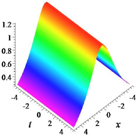
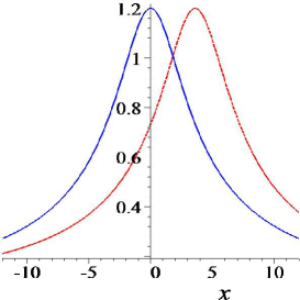
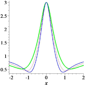
The trajectory of (53) and (54) are two lines defined by $x=-4(\alpha_{1}^{2}-\beta_{1}^{2})t$ and $x=4\beta_{1}^{2}t$ respectively. The profiles of them are depicted in Fig. 1. From Fig. 1 (c), we find the rational single-soliton solution is narrower than the usual single-soliton solution with the same parameters.

Comparing with the solutions of the DNLSI equation generated by DT [23], these two solutions and their modulses are able to be obtained from the corresponding solutions of the DNLSI equation by inverse gauge transformation (3), because integral in (3) containing square of modulus of solutions are indeed calculable explicitly. This is consistent with the known assertion mentioned in the introduction. So we omit the discussion about higher order soliton solutions of the DNLSII equation.

3.2 Breathers from a periodic seed by Darboux transformation

Here, we shall discuss the solutions of the DNLSII equation generated from a periodic solution. In general, set a periodic seed

$$q=c\,{\rm e}^{({\rm i}\rho)},\quad\rho=ax+bt,\quad b=-a^{2}-c^{2}a,\quad a,\ c\in\mathbb{R}.$$ (55)

According to remark 1, $H={{\rm exp}({-\frac{1}{4}\,{\rm i}{c}^{2}\left(4\,ta+{c}^{2}t-2\,x\right)})}$ in this case. Solving the Lax pair (5) associated with this seed solution, and separating variables, we get two different solutions corresponding to an eigenfunction $\lambda$ as

$$\Psi_{1} =\left(\begin{matrix}\psi_{11}(x,t,\lambda)\\ \psi_{12}(x,t,\lambda)\end{matrix}\right)=\left(\begin{matrix}{\frac{2\,{\rm i}a+4\,{\rm i}{\lambda}^{2}-{\rm i}{c}^{2}+{\rm i}s}{4\lambda}}{\rm exp}\left({\rm i}\left(\frac{\rho}{2}-\frac{s}{4}x+\frac{\left(2a+c^{2}-4\lambda^{2}\right)s}{8}t\right)\right)\\ c\,{\rm exp}\left({\rm i}\left(-\frac{\rho}{2}-\frac{s}{4}x+\frac{\left(2a+c^{2}-4\lambda^{2}\right)s}{8}t\right)\right)\end{matrix}\right),$$ (56)

$$\Psi_{2} =\left(\begin{matrix}\psi_{21}(x,t,\lambda)\\ \psi_{22}(x,t,\lambda)\end{matrix}\right)=\left(\begin{matrix}{\frac{2\,{\rm i}a+4\,{\rm i}{\lambda}^{2}-{\rm i}{c}^{2}-{\rm i}s}{4\lambda}}{\rm exp}\left({\rm i}\left(\frac{\rho}{2}+\frac{s}{4}x-\frac{\left(2a+c^{2}-4\lambda^{2}\right)s}{8}t\right)\right)\\ c\,{\rm exp}\left({\rm i}\left(-\frac{\rho}{2}+\frac{s}{4}x-\frac{\left(2a+c^{2}-4\lambda^{2}\right)s}{8}t\right)\right)\end{matrix}\right)$$

with

$$s=\sqrt{4\,{a}^{2}+16\,a{\lambda}^{2}-4\,{c}^{2}a+16\,{\lambda}^{4}+8\,{\lambda}^{2}{c}^{2}+{c}^{4}}.$$ (57)

In condition of $r=q^{*}$, it is obvious that $\left(\begin{matrix}\psi^{*}_{12}(x,t,-\lambda^{*})\\ \psi^{*}_{11}(x,t,-\lambda^{*})\end{matrix}\right)$ and $\left(\begin{matrix}\psi^{*}_{22}(x,t,-\lambda^{*})\\ \psi^{*}_{21}(x,t,-\lambda^{*})\end{matrix}\right)$ are also solutions of the Lax pair (5) associated with $\lambda$ corresponding to lemma 3. Using the principle of superposition, we select the first solution in (56) to get a new solution of the Lax pair (5) with $\lambda=\lambda_{j}$

$$\Phi_{j}=\left(\begin{matrix}f_{j}(x,t,\lambda_{j})\\ g_{j}(x,t,\lambda_{j})\end{matrix}\right)=\left(\begin{matrix}\psi_{11}(x,t,\lambda_{j})+\psi^{*}_{12}(x,t,-\lambda_{j}^{*})\\ \psi_{12}(x,t,\lambda_{j})+\psi^{*}_{11}(x,t,-\lambda_{j}^{*})\\ \end{matrix}\right).$$ (58)

Next, we shall use this eigenfunction to construct new solutions of the DNLSII equation by means of theorems 1 and 2 under the choices of eigenvalues in eq.(50), or equivalently through theorem 5.
Case A: $n=1$. Let $\lambda_{1}={\rm i}{\beta}$, the first order solution is obtained through theorem 1 and eq.(50).

$$q^{[1]}=\left(2\beta+\frac{2ac-4\beta^{2}c-c^{3}+cs_{1}+4\beta{c^{2}}\Gamma_{1}}{(2a-4\beta^{2}-c^{2}+s_{1})\Gamma_{1}+4\beta{c}}\right){{\rm exp}({-\frac{1}{4}\,{\rm i}{c}^{2}\left(t{c}^{2}-2\,x+4\,ta\right)})}$$ (59)

with

$$\Gamma_{1} =\exp\left(2{\rm i}s_{1}\left(-\frac{x}{4}+\frac{(2a+c^{2}+4\beta^{2})t}{8}\right)\right),$$

$$s_{1} =\sqrt{4\,{a}^{2}-16\,a{\beta}^{2}-4\,{c}^{2}a+16\,{\beta}^{4}-8\,{\beta}^{2}{c}^{2}+{c}^{4}}.$$

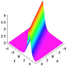
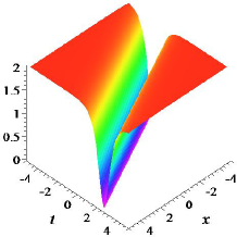
In the case $4\,{a}^{2}-16\,a{\beta}^{2}-4\,{c}^{2}a+16\,{\beta}^{4}-8\,{\beta}^{2}{c}^{2}+{c}^{4}<0$, $q^{[1]}$ gives a soliton solution, which reaches its amplitude $|q_{A}^{[1]}|=|2\beta+c|$ at $x=\frac{2a+c^{2}+4\beta^{2}}{2}t$. When $x\rightarrow\infty,\,t\rightarrow\infty$, $|q_{B}^{[1]}|=|2\beta+{\frac{2\,a-4\,{\beta}^{2}-{c}^{2}+s_{1}}{4\beta}}|$. If $|q_{B}^{[1]}|>|q_{A}^{[1]}|$, it generates a dark soliton. Otherwise, it gives a bright soliton with a non-vanishing boundary. Moreover, $q^{[1]}$ generates a periodic solution while $4\,{a}^{2}-16\,a{\beta}^{2}-4\,{c}^{2}a+16\,{\beta}^{4}-8\,{\beta}^{2}{c}^{2}+{c}^{4}>0$. The dark soliton and bright soliton are showed in Fig. 2.
Case B: $n=2$. To preserve the reduction condition $r^{[2]}={q^{[2]}}^{*}$, set $\lambda_{1}=\alpha_{1}+{\rm i}\beta_{1}\,\mbox{and }\lambda_{2}=-\lambda_{1}^{*}=-\alpha_{1}+{\rm i}\beta_{1}\,(\alpha_{1}\neq 0)$, then $f_{2}=g_{1}^{*},\ g_{2}=f_{1}^{*}$ according to lemma 3 and theorem 5. In order to compare with the breather solution of the DNLSI equation in [23], let $a=-2\,{\alpha_{{1}}}^{2}+2\,{\beta_{{1}}}^{2}-\frac{1}{2}\,{c}^{2}$ such that the imaginary part of ${4\,{a}^{2}+16\,a{\lambda_{1}}^{2}-4\,{c}^{2}a+16\,{\lambda_{1}}^{4}+8\,{\lambda_{1}}^{2}{c}^{2}+{c}^{4}}$ equals $0$. (26) in theorem 2 gives a breather solution of the DNLSII equation as follows:

$$q_{1}^{[2]}=\frac{L_{1}L_{3}}{L_{2}}$$ (60)

with

$$K= 2\,\sqrt{{c}^{4}+4\,{\alpha_{{1}}}^{2}{c}^{2}-4\,{\beta_{{1}}}^{2}{c}^{2}-16\,{\alpha_{{1}}}^{2}{\beta_{{1}}}^{2}},$$

$$L_{1}= A_{1}\sin\Theta_{1}+A_{2}\cos\Theta_{1}+A_{3}\sinh\Theta_{2}+A_{4}\cosh\Theta_{2},$$

$$L_{2}= B_{1}\sin\Theta_{1}+B_{2}\cos\Theta_{1}+B_{3}\sinh\Theta_{2}+B_{4}\cosh\Theta_{2},$$

$$L_{3}= \,{\rm exp}({\rm i}(\tilde{a}x+\tilde{b}t)),\quad\Theta_{1}=\frac{1}{2}K\left(x+4\left(\alpha_{1}^{2}-\beta_{1}^{2}\right)t\right),\quad\Theta_{2}=2K\alpha_{1}\beta_{1}t,$$

$$A_{1}= \,{\rm i}\alpha_{{1}}\beta_{{1}}{c}\left(8\,{\beta_{{1}}}^{2}-2\,{c}^{2}+K\right),\ \ A_{2}=\alpha_{{1}}\beta_{{1}}{c}\left(8\,{\alpha_{{1}}}^{2}+2\,{c}^{2}-K\right),$$

$$A_{3}= \frac{1}{2}{\rm i}\beta_{{1}}\left(8\,{\beta_{{1}}}^{2}-2\,{c}^{2}+K\right)\left(8\,{\alpha_{{1}}}^{2}+{c}^{2}\right),\ A_{4}=\frac{1}{2}\,\alpha_{{1}}\left(8\,{\alpha_{{1}}}^{2}+2\,{c}^{2}-K\right)\left({c}^{2}-8\,{\beta_{{1}}}^{2}\right),$$

$$B_{1}= \,{\rm i}\alpha_{{1}}\beta_{{1}}\left(8\,{\beta_{{1}}}^{2}-2\,{c}^{2}+K\right),\ B_{2}=-\alpha_{{1}}\beta_{{1}}\left(8\,{\alpha_{{1}}}^{2}+2\,{c}^{2}-K\right),$$

$$B_{3}= -\frac{1}{2}{\rm i}{c}\beta_{{1}}\left(8\,{\beta_{{1}}}^{2}-2\,{c}^{2}+K\right),\ B_{4}=\frac{1}{2}\,{c}\alpha_{{1}}\left(8\,{\alpha_{{1}}}^{2}+2\,{c}^{2}-K\right),$$

$$\tilde{a}= (-2\,{\alpha_{{1}}}^{2}+2\,{\beta_{{1}}}^{2}-\frac{1}{2}\,{c}^{2}),\ \tilde{b}=(-4\,{\alpha_{{1}}}^{4}+8\,{\alpha_{{1}}}^{2}{\beta_{{1}}}^{2}-4\,{\beta_{{1}}}^{4}+\frac{1}{4}\,{c}^{4}).$$

If $K^{2}<0$, it reaches its amplitude $|c+4\beta_{1}|$ at $x=4(\,\beta_{1}^{2}-\,\alpha_{1}^{2})t$, i.e., it propagates along a line in the direction $x=4(\,\beta_{1}^{2}-\,\alpha_{1}^{2})t$ on ($x,t$)-plane. Especially, when $|\alpha_{1}|=|\beta_{1}|$, the temporal periodic breather solution (Kuznetsov-Ma breather [63, 64]) is obtained. If $K^{2}>0$, it reaches its amplitude $|c+4\beta_{1}|$ at $t=0$, i.e., the spacial periodic breather solution (Akhmediev breather [39]). Three kinds of breather solutions are shown in Fig. 3 to confirm their periodicity. Furthermore, in order to compare with the result [23] of the DNLSI equation, we present an expression of the square of the modulus of a breather solution given by (60) as

$${|q_{1}^{[2]}|}^{2}=\frac{\widetilde{L_{1}}}{\widetilde{L_{2}}},$$ (61)

with

$$\qquad\widetilde{L_{1}}= \widetilde{A_{1}}\sin\Theta_{1}\sinh\Theta_{2}+\widetilde{A_{2}}\cos\Theta_{1}\cosh\Theta_{2}+\widetilde{A_{3}}\cos(2\Theta_{1})+\widetilde{A_{4}}\cosh(2\Theta_{2})+\widetilde{A_{5}},$$

$$\qquad\widetilde{L_{2}}= \widetilde{B_{1}}\sin\Theta_{1}\sinh\Theta_{2}+\widetilde{B_{2}}\cos\Theta_{1}\cosh\Theta_{2}+\widetilde{B_{3}}\cos(2\Theta_{1})+\widetilde{B_{4}}\cosh(2\Theta_{2})+\widetilde{B_{5}},$$

$$\widetilde{A_{1}}= (\alpha_{{1}}{\beta_{{1}}}^{2}{c}^{3}+8\,{\alpha_{{1}}}^{3}{\beta_{{1}}}^{2}c){k_{{1}}}^{2},\widetilde{A_{2}}=({\alpha_{{1}}}^{2}\beta_{{1}}{c}^{3}-8\,{\alpha_{{1}}}^{2}{\beta_{{1}}}^{3}c){k_{{2}}}^{2},\widetilde{A_{3}}=\frac{1}{2}\,{\alpha_{{1}}}^{2}{\beta_{{1}}}^{2}{c}^{2}\left({k_{{2}}}^{2}-{k_{{1}}}^{2}\right),$$

$$\widetilde{A_{4}}= \frac{1}{8}\,{c}^{4}\left({\beta_{{1}}}^{2}{k_{{1}}}^{2}+{\alpha_{{1}}}^{2}{k_{{2}}}^{2}\right)+8\,{\alpha_{{1}}}^{2}{\beta_{{1}}}^{2}\left({\alpha_{{1}}}^{2}{k_{{1}}}^{2}+{\beta_{{1}}}^{2}{k_{{2}}}^{2}\right)+2\,{\alpha_{{1}}}^{2}{\beta_{{1}}}^{2}{c}^{2}\left({k_{{1}}}^{2}+{k_{{2}}}^{2}\right),$$

$$\widetilde{A_{5}}= \frac{1}{8}\,{c}^{4}\left({\alpha_{{1}}}^{2}{k_{{2}}}^{2}-{\beta_{{1}}}^{2}{k_{{1}}}^{2}\right)+8\,{\alpha_{{1}}}^{2}{\beta_{{1}}}^{2}\left({\beta_{{1}}}^{2}{k_{{2}}}^{2}-{\alpha_{{1}}}^{2}{k_{{1}}}^{2}\right)-\frac{3}{2}\,{\alpha_{{1}}}^{2}{\beta_{{1}}}^{2}{c}^{2}\left({k_{{1}}}^{2}+{k_{{2}}}^{2}\right),$$

$$\widetilde{B_{1}}= -c\alpha_{{1}}{\beta_{{1}}}^{2}{k_{{1}}}^{2},\ \widetilde{B_{2}}=-c{\alpha_{{1}}}^{2}\beta_{{1}}{k_{{2}}}^{2},\ \widetilde{B_{3}}=\frac{1}{2}\,{\alpha_{{1}}}^{2}{\beta_{{1}}}^{2}\left({k_{{2}}}^{2}-{k_{{1}}}^{2}\right),$$

$$\widetilde{B_{4}}= \frac{1}{8}\,{c}^{2}\left({\beta_{{1}}}^{2}{k_{{1}}}^{2}+{\alpha_{{1}}}^{2}{k_{{2}}}^{2}\right),\ \widetilde{B_{5}}=\frac{1}{8}\,{c}^{2}\left({\alpha_{{1}}}^{2}{k_{{2}}}^{2}-{\beta_{{1}}}^{2}{k_{{1}}}^{2}\right)+\frac{1}{2}\,{\alpha_{{1}}}^{2}{\beta_{{1}}}^{2}\left({k_{{1}}}^{2}+{k_{{2}}}^{2}\right),$$

$$k_{1}= 8\,{\beta_{{1}}}^{2}-2\,{c}^{2}+K,\ k_{2}=8\,{\alpha_{{1}}}^{2}+2\,{c}^{2}-K.$$

It is obvious that ${|q_{1}^{[2]}|}^{2}$ is different from the square of modulus of a breather (see eq.(53) of ref.[23]) for the DNLSI equation. So $q_{1}^{[2]}$ can not be obtained from the above mentioned breather of the DNLSI equation by the gauge transformation (3) because this transformation keeps the modulus of two solutions invariant.

Note that the period of the breather solution (60) is proportional to $\frac{1}{K}$. Let $K$ go to zero, then the period of the breather goes to infinity and leave only one peak located around the origin of the $(x,\,t)$-plane. Since $c=2\beta_{1}$ is a common zero of $K$ and the eigenfunction $\Phi_{1}$ in (58), $q_{1}^{[2]}$ in (60) becomes an indeterminate form $\frac{0}{0}$. By adopting L’Hospital’s rule for this breather solution at $c=2\beta_{1}$, we obtain the first order rogue wave solution $q^{[2]}_{2}$ of the DNLSII equation:

$$q^{[2]}_{2}=-\frac{L_{1}}{L_{2}}2\beta_{1}{\rm exp}\left({-2\,{\rm i}{\alpha_{{1}}}^{2}\left(x+2\,t{\alpha_{{1}}}^{2}-4\,t{\beta_{{1}}}^{2}\right)}\right),$$ (62)

with

$$L_{1}= 16\,{\rm i}{\beta_{{1}}}^{4}{x}^{2}+16\,{\rm i}{\alpha_{{1}}}^{2}{\beta_{{1}}}^{2}{x}^{2}-128\,{\rm i}{\beta_{{1}}}^{6}xt+128\,{\rm i}{\beta_{{1}}}^{2}t{\alpha_{{1}}}^{4}x+8\,{\beta_{{1}}}^{2}x$$

$$+96\,t{\alpha_{{1}}}^{2}{\beta_{{1}}}^{2}+256\,{\rm i}{\beta_{{1}}}^{2}{t}^{2}{\alpha_{{1}}}^{6}-3\,{\rm i}+256\,{\rm i}{\beta_{{1}}}^{8}{t}^{2},$$

$$L_{2}= 16\,{\rm i}{\alpha_{{1}}}^{2}{\beta_{{1}}}^{2}{x}^{2}+16\,{\rm i}{\beta_{{1}}}^{4}{x}^{2}+128\,{\rm i}{\beta_{{1}}}^{2}t{\alpha_{{1}}}^{4}x-128\,{\rm i}{\beta_{{1}}}^{6}xt-8\,{\beta_{{1}}}^{2}x$$

$$+256\,{\rm i}{\beta_{{1}}}^{2}{t}^{2}{\alpha_{{1}}}^{6}+256\,{\rm i}{\beta_{{1}}}^{8}{t}^{2}-32\,t{\alpha_{{1}}}^{2}{\beta_{{1}}}^{2}+{\rm i}+64\,t{\beta_{{1}}}^{4}.$$

While $x$ (or $t$) goes to infinity, $|q_{2}^{[2]}|^{2}$ goes to $4\beta_{1}^{2}$. The maximum amplitude of $|q_{2}^{[2]}|^{2}$ equals to $36\beta_{1}^{2}$ locating at $(0,\,0)$, and the minimum amplitude of $|q_{2}^{[2]}|^{2}$ is $0$ locating at $(\,{\frac{3\sqrt{3}{\alpha_{{1}}}^{2}}{4\sqrt{4\,{\alpha_{{1}}}^{2}+{\beta_{{1}}}^{2}}\left({\alpha_{{1}}}^{2}+{\beta_{{1}}}^{2}\right)\beta_{{1}}}}$,
$-{\frac{\sqrt{3}}{16\sqrt{4\,{\alpha_{{1}}}^{2}+{\beta_{{1}}}^{2}}\left({\alpha_{{1}}}^{2}+{\beta_{{1}}}^{2}\right)\beta_{{1}}}})$ and $(-\,{\frac{3\sqrt{3}{\alpha_{{1}}}^{2}}{4\sqrt{4\,{\alpha_{{1}}}^{2}+{\beta_{{1}}}^{2}}\left({\alpha_{{1}}}^{2}+{\beta_{{1}}}^{2}\right)\beta_{{1}}}},\,{\frac{\sqrt{3}}{16\sqrt{4\,{\alpha_{{1}}}^{2}+{\beta_{{1}}}^{2}}\left({\alpha_{{1}}}^{2}+{\beta_{{1}}}^{2}\right)\beta_{{1}}}})$. 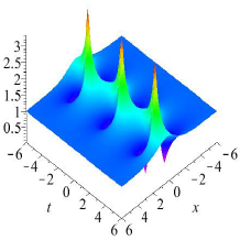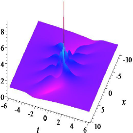Two figures of the rogue wave solution (62) with special parameters are displayed in Fig. 4 in order to show its typical features: localized profile on whole plane and a remarkable peak over asymptotical plane.

Note that the first order rogue wave solution $q^{[2]}_{2}$ of the DNLSII equation is different from the rogue wave of the DNLSI equation (see eq.(56) of ref.[23]). The degree of the polynomial in denominator for the latter is four, which is double of former. But the transformation (3) can not change this degree of two related functions. Nevertheless, the modulus of above mentioned two first order rogue waves are the same. That is, they possess the same asymptotical plane and amplitude.

3.3 Rogue waves from breathers by higher order Taylor expansion

In this subsection, we shall construct higher order rogue waves of the DNLSII equation according to theorems 4 and 5 under double degeneration [44] including eigenvalue degeneration $\lambda_{j}\rightarrow\lambda_{0}$ $(j=1,3,5,\dots,2k-1)$ and eigenfunction degeneration $\Phi_{j}(\lambda_{0})=0$ in $T_{n}$ with $n=2k$.

According to the principle of linear superposition and lemma 3, we construct a new general eigenfunction associated with $\lambda_{j}$ as

$$\Phi_{j}=\left(\begin{matrix}f_{j}(x,t,\lambda_{j})\\ g_{j}(x,t,\lambda_{j})\end{matrix}\right)=\left(\begin{matrix}C_{1}\psi_{11}(x,t,\lambda_{j})+C_{2}{{\psi}_{12}}^{*}(x,t,-{\lambda_{j}}^{*})\\ C_{1}\psi_{12}(x,t,\lambda_{j})+C_{2}{{\psi}_{11}}^{*}(x,t,-{\lambda_{j}}^{*})\\ \end{matrix}\right),$$ (63)

from $\Psi_{1}(\lambda)$ in (56). Here two superposition coefficients are $C_{1}={\rm exp}\left({\rm i}s\sum_{0}^{k-1}\epsilon^{2m}l_{m}\right),\ C_{2}={\rm exp}\left({\rm-i}s\sum_{0}^{k-1}\epsilon^{2m}l_{m}\right),\ m=0,1,2,3\cdots k-1,l_{m}\in\mathbb{C}$. If $l_{m}=0$ $(m=0,1,2,\cdots,k-1)$, $\Phi_{j}$ in (63) is the same as that in (58). Note that $\Phi_{j}$ $(j=1,3,5,\cdots,2k-1)$ have the same expression derived from (56) with different eigenvalues $\lambda_{j}$. This fact is important to guarantee the degeneration of $T_{n}$ when eigenvalues are the same as a special one $\lambda_{0}$.

It is not difficult to check that $\lambda_{0}=\sqrt{\frac{-a}{2}}+{\rm i}c$ $(a<0)$ is only one common zero of eigenfunctions $\Phi_{j}$ in (63) and $s$ in (57). When $\Phi_{j}$ be given by (63), let $\lambda_{j}\to\lambda_{0}$, then theorem 4, theorem 5 and corollary 1 imply that double degeneration occurs in $T_{n}$, and $q^{[n]}$ is of indeterminate form $\frac{0}{0}$. By higher order Taylor expansion as in [29, 65, 66, 67, 68, 69, 70, 71], $q^{[n]}$ generates the $k$-th order rogue wave of the DNLSII equation. Here $n=2k$.

Theorem 6.

Set $n=2k$, $j=1,3,5,\dots,k$, $a<0$, $\lambda_{j}=\sqrt{\frac{-a}{2}}+{\rm i}c+\epsilon^{2}$. Let $\Phi_{j}$ be given by (63). The $k$-th order rogue wave solution for the DNLSII equation is expressed by

$$q^{[n]}=\frac{|\widehat{W_{n}}^{\prime}|}{|W_{n}^{\prime}|}q-2{\rm i}\frac{|M_{n}^{\prime}|}{|W_{n}^{\prime}|}$$ (64)

with

$$\widehat{W_{n}}^{\prime}= \left(\left.\frac{\partial^{n_{i}}}{\partial\epsilon^{n_{i}}}\right|_{\epsilon=0}(\widehat{W_{n}})_{ij}(\lambda_{0}+\epsilon^{2})\right)_{n\times n},$$ (65)

$${W_{n}}^{\prime}= \left(\left.\frac{\partial^{n_{i}}}{\partial\epsilon^{n_{i}}}\right|_{\epsilon=0}\left({W_{n}}\right)_{ij}(\lambda_{0}+\epsilon^{2})\right)_{n\times n},$$

$${M_{n}}^{\prime}= \left(\left.\frac{\partial^{n_{i}}}{\partial\epsilon^{n_{i}}}\right|_{\epsilon=0}\left({M_{n}}\right)_{ij}(\lambda_{0}+\epsilon^{2})\right)_{n\times n}.$$

Here $n_{i}=i$ if $i$ is odd and $n_{i}=i-1$ if $i$ is even. This solution has free parameters $a,c,l_{i}$ $(i=0,1,2,\cdots,k-1)$.

For convenience, let $a=-1$ and $c=1$ in following all rogue waves. Let $n=4$, $l_{0}=0$ in theorem 6. The second order rogue wave of the DNLSII equation is given by

$$q^{[4]}=\frac{L_{1}}{L_{2}}{\rm exp}(-{\rm i}x),$$ (66)

where

$$L_{1}= -15-9\,{x}^{6}-243\,{t}^{6}+81\,{x}^{2}+207\,{t}^{2}+1323\,{t}^{4}+39\,{x}^{4}+1296\,{\rm i}{x}^{2}{t}^{3}$$

$$+1458\,{\rm i}x{t}^{4}+180\,{\rm i}{x}^{4}t+612\,{\rm i}{t}^{2}{x}^{3}-54\,{x}^{5}t-567\,{t}^{4}{x}^{2}-486\,{t}^{5}x$$

$$-396\,{t}^{3}{x}^{3}-189\,{x}^{4}{t}^{2}-54\,xt+1242\,{x}^{2}{t}^{2}+2052\,x{t}^{3}+276\,{x}^{3}t-30\,{\rm i}x$$

$$-216\,{\rm i}{t}^{3}-28\,{\rm i}{x}^{3}-228\,{\rm i}t-288\,{\rm i}{x}^{2}t-972\,{\rm i}x{t}^{2}+18\,{\rm i}{x}^{5}+972\,{\rm i}{t}^{5}$$

$$+(324\,\sqrt{2}{x}^{2}t-216\,{\rm i}xt\sqrt{2}+324\,\sqrt{2}x{t}^{2}-216\,{\rm i}\sqrt{2}{x}^{2}+432\,{\rm i}{t}^{2}\sqrt{2}$$

$$+36\,\sqrt{2}t-108\,\sqrt{2}{t}^{3}+36\,\sqrt{2}{x}^{3}-96\,{\rm i}\sqrt{2}-36\,\sqrt{2}x)l_{{1}}-216\,{l_{{1}}}^{2},$$

$$L_{2}= -3-9\,{x}^{6}-243\,{t}^{6}-39\,{x}^{2}-441\,{t}^{2}-297\,{t}^{4}+3\,{x}^{4}+108\,{\rm i}x{t}^{2}-54\,{x}^{5}t$$

$$-567\,{t}^{4}{x}^{2}-486\,{t}^{5}x-396\,{t}^{3}{x}^{3}-189\,{x}^{4}{t}^{2}-54\,xt+162\,{x}^{2}{t}^{2}+324\,x{t}^{3}$$

$$-12\,{x}^{3}t-18\,{\rm i}{x}^{5}-18\,{\rm i}x-20\,{\rm i}{x}^{3}-162\,{\rm i}x{t}^{4}-216\,{\rm i}{x}^{2}{t}^{3}-72\,{\rm i}{x}^{2}t$$

$$-180\,{\rm i}{t}^{2}{x}^{3}-72\,{\rm i}{x}^{4}t+432\,{\rm i}{t}^{3}+48\,{\rm i}t-216\,{l_{{1}}}^{2}+(216\,{\rm i}xt\sqrt{2}+36$$

$$\ +324\,\sqrt{2}x{t}^{2}+24\,{\rm i}\sqrt{2}-396\,\sqrt{2}t+324\,\sqrt{2}{x}^{2}t+216\,{\rm i}{t}^{2}\sqrt{2}-36\,\sqrt{2}x$$

$$\ -108\,\sqrt{2}{t}^{3})l_{{1}}.$$

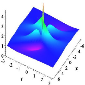
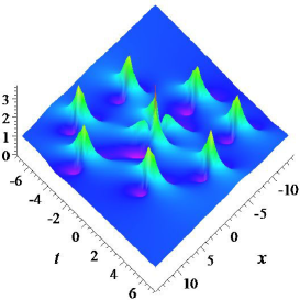
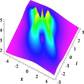
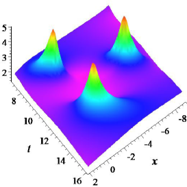
There exists only one free parameter $l_{1}$ in these expressions. Here we have set $l_{0}=0$ without loss of generality, because it only changes the location of the rogue wave with the same profile. Other parameters $l_{j}$ for $j\geq 2$ disappear automatically in $q^{[2]}$ because of the limit $\epsilon\rightarrow 0$. While $l_{1}=0$, we get the fundamental pattern of the second order rogue wave, whose maximum amplitude is equal to $5$ and locates at (0, 0). While $l_{1}=100$, the second order rogue wave splits up into three first order rogue waves rather than two, which locate at approximately $(5.77,\,1.74)$, $(3.63,\,-5.29)$, and $(-9.62,\,3.66)$. The profiles of two second-order rogue wave are plotted in Fig. 5.

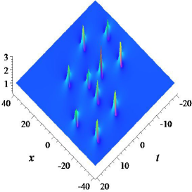
When $n$ increases, more patterns of $k$-th rogue wave solution can be obtained from theorem 6. For instance, when $k=3$, the third order rogue wave with three parameters, i.e. $l_{0},l_{1},l_{2}$, possesses a circular pattern apart from the fundamental pattern and the triangular pattern. Furthermore, set $l_{j}=0$ $(j=0,1,2)$, the third order fundamental pattern of the DNLSII equation is given by

$$q^{[6]}=\frac{L_{1}}{L_{2}}\exp(-{\rm i}x)$$ (67)

with

$$L_{1}= -81\,{x}^{12}-972\,{x}^{11}t-6318\,{x}^{10}{t}^{2}-27540\,{x}^{9}{t}^{3}-88695\,{x}^{8}{t}^{4}-219672\,{x}^{7}{t}^{5}-428004\,{x}^{6}{t}^{6}$$

$$-659016\,{x}^{5}{t}^{7}-798255\,{x}^{4}{t}^{8}-743580\,{x}^{3}{t}^{9}-511758\,{x}^{2}{t}^{10}-236196\,x{t}^{11}-59049\,{t}^{12}$$

$$+324\,{\rm i}{x}^{11}+5184\,{\rm i}{x}^{10}t+37260\,{\rm i}{x}^{9}{t}^{2}+171720\,{\rm i}{x}^{8}{t}^{3}+560520\,{\rm i}{x}^{7}{t}^{4}+1371168\,{\rm i}{x}^{6}{t}^{5}$$

$$+2560248\,{\rm i}{x}^{5}{t}^{6}+3674160\,{\rm i}{x}^{4}{t}^{7}+3980340\,{\rm i}{x}^{3}{t}^{8}+3149280\,{\rm i}{x}^{2}{t}^{9}+1653372\,{\rm i}x{t}^{10}+472392\,{\rm i}{t}^{11}$$

$$+1026\,{x}^{10}+15660\,{x}^{9}t+127170\,{x}^{8}{t}^{2}+619920\,{x}^{7}{t}^{3}+2057940\,{x}^{6}{t}^{4}+4865832\,{x}^{5}{t}^{5}$$

$$+8393220\,{x}^{4}{t}^{6}+10478160\,{x}^{3}{t}^{7}+9163530\,{x}^{2}{t}^{8}+5117580\,x{t}^{9}+1430298\,{t}^{10}-1620\,{\rm i}{x}^{9}$$

$$-29160\,{\rm i}{x}^{8}t-252720\,{\rm i}{x}^{7}{t}^{2}-1296000\,{\rm i}{x}^{6}{t}^{3}-4247640\,{\rm i}{x}^{5}{t}^{4}-9311760\,{\rm i}{x}^{4}{t}^{5}-13860720\,{\rm i}{x}^{3}{t}^{6}$$

$$-13296960\,{\rm i}{x}^{2}{t}^{7}-7479540\,{\rm i}x{t}^{8}-1312200\,{\rm i}{t}^{9}+2745\,{x}^{8}-2520\,{x}^{7}t-194220\,{x}^{6}{t}^{2}$$

$$-1344600\,{x}^{5}{t}^{3}-4167450\,{x}^{4}{t}^{4}-7597800\,{x}^{3}{t}^{5}-9083340\,{x}^{2}{t}^{6}-6561000\,x{t}^{7}-127575\,{t}^{8}$$

$$-8760\,{\rm i}{x}^{7}-85920\,{\rm i}{x}^{6}t-212760\,{\rm i}{x}^{5}{t}^{2}-97200\,{\rm i}{x}^{4}{t}^{3}+113400\,{\rm i}{x}^{3}{t}^{4}+3732480\,{\rm i}{x}^{2}{t}^{5}$$

$$+8135640\,{\rm i}x{t}^{6}+4024080\,{\rm i}{t}^{7}+21020\,{x}^{6}+12600\,{x}^{5}t-56700\,{x}^{4}{t}^{2}-874800\,{x}^{3}{t}^{3}-413100\,{x}^{2}{t}^{4}$$

$$+4791960\,x{t}^{5}+9977580\,{t}^{6}-33480\,{\rm i}{x}^{5}-313200\,{\rm i}{x}^{4}t-630000\,{\rm i}{x}^{3}{t}^{2}-1425600\,{\rm i}{x}^{2}{t}^{3}$$

$$-3450600\,{\rm i}x{t}^{4}-9545040\,{\rm i}{t}^{5}-41775\,{x}^{4}-318300\,{x}^{3}t-2031750\,{x}^{2}{t}^{2}-3410100\,x{t}^{3}$$

$$-3983175\,{t}^{4}+16500\,{\rm i}{x}^{3}+237600\,{\rm i}{x}^{2}t+1147500\,{\rm i}x{t}^{2}-1171800\,{\rm i}{t}^{3}-28350\,{x}^{2}+121500\,xt$$

$$-166950\,{t}^{2}+6300\,{\rm i}x+63000\,{\rm i}t+1575,$$

$$L_{2}= 81\,{x}^{12}+972\,{x}^{11}t+6318\,{x}^{10}{t}^{2}+27540\,{x}^{9}{t}^{3}+88695\,{x}^{8}{t}^{4}+219672\,{x}^{7}{t}^{5}+428004\,{x}^{6}{t}^{6}$$

$$+659016\,{x}^{5}{t}^{7}+798255\,{x}^{4}{t}^{8}+743580\,{x}^{3}{t}^{9}+511758\,{x}^{2}{t}^{10}+236196\,x{t}^{11}+59049\,{t}^{12}$$

$$+324\,{\rm i}{x}^{11}+3240\,{\rm i}{x}^{10}t+17820\,{\rm i}{x}^{9}{t}^{2}+64800\,{\rm i}{x}^{8}{t}^{3}+171720\,{\rm i}{x}^{7}{t}^{4}+340848\,{\rm i}{x}^{6}{t}^{5}$$

$$+515160\,{\rm i}{x}^{5}{t}^{6}+583200\,{\rm i}{x}^{4}{t}^{7}+481140\,{\rm i}{x}^{3}{t}^{8}+262440\,{\rm i}{x}^{2}{t}^{9}+78732\,{\rm i}x{t}^{10}-378\,{x}^{10}$$

$$-2700\,{x}^{9}t-20250\,{x}^{8}{t}^{2}-101520\,{x}^{7}{t}^{3}-340740\,{x}^{6}{t}^{4}-775656\,{x}^{5}{t}^{5}-1180980\,{x}^{4}{t}^{6}$$

$$-1146960\,{x}^{3}{t}^{7}-503010\,{x}^{2}{t}^{8}+131220\,x{t}^{9}+301806\,{t}^{10}+540\,{\rm i}{x}^{9}+6480\,{\rm i}{x}^{8}t+6480\,{\rm i}{x}^{7}{t}^{2}$$

$$-73440\,{\rm i}{x}^{6}{t}^{3}-372600\,{\rm i}{x}^{5}{t}^{4}-933120\,{\rm i}{x}^{4}{t}^{5}-1419120\,{\rm i}{x}^{3}{t}^{6}-1516320\,{\rm i}{x}^{2}{t}^{7}-1006020\,{\rm i}x{t}^{8}$$

$$-524880\,{\rm i}{t}^{9}+495\,{x}^{8}+2520\,{x}^{7}t+51660\,{x}^{6}{t}^{2}+255960\,{x}^{5}{t}^{3}+506250\,{x}^{4}{t}^{4}+443880\,{x}^{3}{t}^{5}$$

$$+2201580\,{x}^{2}{t}^{6}+4228200\,x{t}^{7}+3189375\,{t}^{8}+5640\,{\rm i}{x}^{7}+35760\,{\rm i}{x}^{6}t+145800\,{\rm i}{x}^{5}{t}^{2}$$

$$+324000\,{\rm i}{x}^{4}{t}^{3}-145800\,{\rm i}{x}^{3}{t}^{4}-3013200\,{\rm i}{x}^{2}{t}^{5}-3411720\,{\rm i}x{t}^{6}-2099520\,{\rm i}{t}^{7}+12340\,{x}^{6}$$

$$+70920\,{x}^{5}t+369900\,{x}^{4}{t}^{2}+874800\,{x}^{3}{t}^{3}+4009500\,{x}^{2}{t}^{4}+7727400\,x{t}^{5}+4544100\,{t}^{6}$$

$$+23640\,{\rm i}{x}^{5}+43200\,{\rm i}{x}^{4}t+61200\,{\rm i}{x}^{3}{t}^{2}-842400\,{\rm i}{x}^{2}{t}^{3}+631800\,{\rm i}x{t}^{4}+583200\,{\rm i}{t}^{5}-7425\,{x}^{4}$$

$$+30300\,{x}^{3}t-322650\,{x}^{2}{t}^{2}+40500\,x{t}^{3}+2330775\,{t}^{4}+11700\,{\rm i}{x}^{3}+23400\,{\rm i}{x}^{2}t-245700\,{\rm i}x{t}^{2}$$

$$-993600\,{\rm i}{t}^{3}+8550\,{x}^{2}+900\,xt+291150\,{t}^{2}+2700\,{\rm i}x-18000\,{\rm i}t+225.$$

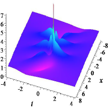
All patterns of the third order rogue are displayed in Fig. 6 by using formula (64).

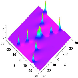
Set $k=4$ in theorem 6, then $q^{[8]}$ in (64) gives the fourth order rogue wave of the DNLSII equation. This solution possesses as least four patterns: a fundamental pattern, a triangular pattern, a circular-fundamental pattern and a circular-triangular pattern. These four patterns of rogue wave are displayed in Fig. 7 by using formula (64).

All the above-mentioned rogue waves are plotted by using the analytical formulas according to theorem 6. Their validity has been confirmed analytically by a simple symbolic computation. In addition, we have got explicit expressions of other higher order rogue waves and their figures. However, they are too long to write out here. Based on these figures and analytical formulas of the rogue waves, we can provide following conjectures for the DNLSII equation.

Remark 2.

• 1) Under the fundamental pattern, the height of above-mentioned four rogue waves is 3, 5, 7, 9, respectively. We conjecture that the maximum amplitude of the $k$-th order rogue wave of the DNLSII equation is $(2k+1)c$. Here $c$ is the asymptotical height of rogue wave.

• 2) The degree of the polynomials in above-mentioned four rogue waves is 2, 6, 12, 20 respectively. We conjecture that the degree of the polynomials in the $k$-th order rogue wave of the DNLSII equation is $k(k+1)$.

• 3) The maximum number of peaks in above-mentioned four rogue waves is 1, 3, 6, 10, respectively. We conjecture that the $k$-th order rogue wave of the DNLSII equation can be decomposed thoroughly into $\dfrac{k(k+1)}{2}$ first order rogue waves.

• 4) From Figs.6(c),7(c) and 7(d), we conjecture that the $k$-th order rogue wave of the DNLSII equation can be decomposed into a pattern of a $(k-2)$-th order rogue wave plus an outer ring on which there are $2k-1$ first-order rogues. Note that the central profile of these three figures is a first-order rogue wave, a fundamental pattern and a triangular pattern of the second-order rogue wave, respectively.
  

These conjectures can be regarded as natural extensions of the counterparts [41, 42, 49, 50] for the NLS equation. It is worth mentioning again that the item 2 is not true for the DNLSI equation. This fact shows again that rogue waves of this equation can not be obtained by transformation (3) from rogue waves of the DNLSI equation, because transformation (3) does not change the degree in two related solutions.

4. Conclusion and discussion

In this paper, the DNLSII equation, which is an important model to describe the propagation of light pulse involving self-steepening without concomitant self-phase-modulation [17], has been studied from the point of view of the analytical theory for integrable systems. The main results of the paper are:
1) Present the determinant representation $T_{n}$ of the coupled DNLSII equations (theorem 4);
2) Under choice (50) on the eigenvalues and eigenfunctions, $T_{n}$ is reduced to the $n$-fold DT of the DNLSII equation and $q^{[n]}$ generated by this reduced $T_{n}$ is a solution of it (theorem 5);
3) Obtain an analytical formula of the $k$-th order rogue waves for the DNLSII equation (theorem 6).
In addition, several breathers and lower order rogue waves are given through analytical expressions and their profiles are plotted analytically in figures. As $n$-times iteration of the $T_{1}$, these $T_{n}$ of the DNLSII equation include complicated integrals like $\int q^{[j-1]}r^{[j-1]}\mathrm{d}x$ $(j=1,2,\cdots,n)$. To our best knowledge, this kind of DT is unusual by comparing with known DT for soliton equations. These integrals are not calculable explicitly in general case, and thus result in a remarkable difficulty to construct $T_{n}$ in terms of determinants and to get explicit solutions of the DNLSII equation. We have introduced functions $H^{[i]}$ $(i=0,1,2,\cdots,n-1)$ and proved that $\dfrac{g^{[k]}_{i}}{f^{[k]}_{i}}H^{[k+1]}$ is a constant for $i\geq k+1$ in theorem 3. Finally, we have eliminated these unfavorable integrals in $T_{n}$ by using this crucial fact.

It is a well-accepted idea [55, 56] in the research community of the mathematical physics that an integrable model can be solved by means of DT. From this sense, the DNLSII equation, which was introduced as an integrable model at 1979 [1], is a rare exceptional example because its DT has not been established over the past 30 years. Thus, it is a long-standing problem to construct the DT of this equation. We have solved this problem by establishment of the determinant representation of $T_{n}$ in theorems 4 and 5 for the DNLSII equation. Moreover, breather in (61) and rogue waves in eqs.(62),(66) and (67), can not be obtained from counterparts of the DNLSI equation by gauge transformation (3). This observation shows that it is necessary to get explicit solution $q$ of the DNLSII equation, and then clarifies a well-known doubt of the necessity for solving DNLSII equation. This doubt originates from gauge transformation (3) [8, 7] between the DNLSII equation and the DNLSI equation.

The solutions presented in this paper have wide relevance of physics because the DNLSII equation is a physical model of light pulses [17]. On the one side, two typical features, i.e. high amplitude (or high energy equivalently in optics) and localized property of the rogue wave pulse, may result in high possibility to observe the self-steepening effect in light pulses. It is difficult to realize this in normal state for nonlinear propagation of light [17]. On the other side, with the solutions in this paper we have a new opportunity to observe optical rogue wave by using the balance between the dispersion and self-steepening instead of the self-phase-modulation in optical fiber. This will be helpful to use and control rogue wave in the future. For example, as in the case of the NLS equation [29], different patterns of the second order rogue wave here can also be controlled by phase modulation at the interaction area of two first order breathers. This can be realized by choosing different values of $l_{0}$ in eigenfunction (63) with $l_{i}=0$ $(i>0)$. More specifically, set $n=4$, $a=-1$, $c=1$, and let $\Phi_{j}$ $(j=1,3)$ be given by (63), then by theorem 5, $q^{[4]}$ in (48) generates a second-order breather $q_{2b}$ of the DNLSII equation with parameters $a,c,\lambda_{1},\lambda_{3}$ and $l_{0}$. Firstly, if $l_{0}=0$ in $\Phi_{1}$ and $\Phi_{3}$, the two breathers in $q_{2b}$ have no phase difference. Set $\lambda_{1}=0.7+0.5{\rm i}$ and $\lambda_{3}=0.75+0.5{\rm i}$ in $q_{2b}$, we get a “fundamental pattern” at interaction area of the second-order breather, which is plotted in fig. 8. It is obvious that the central profile is similar to a fundamental pattern in fig. 5 (a). Secondly, let $l_{0}=6.25$ and $\lambda_{1}=0.68+0.5{\rm i}$ in $\Phi_{1}$, and $l_{0}=-8{\rm i}$ and $\lambda_{3}=0.8+0.5{\rm i}$ in $\Phi_{3}$, then $q_{2b}$ displays a “triangular pattern” at interaction area which is plotted in fig. 9. It is obvious that the central profile is similar to the triangular pattern in fig. 5(b). Of course, we can get more interesting patterns by tuning the phase of breathers at interaction area for higher order case. More detailed studies will be done in the near future.

Further more, based on the DT we constructed, we can study other interesting phenomena in such systems from unstable plane wave background, such as the so-called super-regular solitonic solutions [72], and the integrable soliton turbulence [73]. The study of the evolution of rational rogue waves in DNLSII in presence of an additional noise by a numerical algorithm will be realized in near future [74].
Acknowledgments This work is supported by the NSF of China under Grant No.11271210 and No.11171073, the K. C. Wong Magna Fund in Ningbo University and the Natural Science Foundation of Ningbo under Grant No. 2011A610179. J.S. He thanks sincerely Prof. A.S. Fokas for arranging the visit to Cambridge University in 2012-2014 and for many useful discussions. We thank very much two referee for helpful and detailed suggestions on our initial submission.

$|q_{1}^{[2]}|\,$   $|q_{2}^{[2]}|\,$
$|q_{1}^{[2]}|\&|q_{2}^{[2]}|\,$   $|q_{2}^{[2]}|\,$

Figure 1. Profiles of the singles-solitons generated from a vacuum solution. (a) A usual single-soliton with $\alpha_{1}=0.3,\,\beta_{1}=0.3$ locating near $x=0$. (b) A rational single-soliton with $\beta_{1}=0.3$ locating near $x=0.36t$. (c) A usual single-soliton (the green dot line) and a rational single-soliton (the blue solid line) at $t=0$. They possess the same amplitude, but the rational single-soliton is steeper than the usual one. (d) The rational single-soliton at $t=0$ (the blue solid line) and $t=10$ (the red dash line). The blue line reaches its peak at $x=0$, the red one at $x=3.6$.

${|q^{[1]}|}^{2}\,$  ${|q^{[1]}|}^{2}\,$  ${|q^{[1]}|}^{2}\,$

Figure 2. Profiles of single-solitons generated from a periodic seed. (a) A bright soliton with $a=1,\,c=1$ and $\beta=0.5$. (b) A dark soliton with $a=1,\,c=1$ and $\beta=-0.5$. (c) The graphical superposition of a bright soliton and a dark soliton at $t=0$. Both the bright soliton and the dark soliton achieve their peaks at the same time, and share the same non-vanishing boundary condition.

${|q_{1}^{[2]}|}\,$  ${|q_{1}^{[2]}|}\,$  ${|q_{1}^{[2]}|}\,$

Figure 3. The evolution of three breathers. (a) A temporal periodic breather with $\alpha_{1}=0.6,\,\beta_{1}=0.6$ and $c=1$. (b) A breather with a certain angle with $x$-axis and $t$-axis under specific parameters $\alpha_{1}=0.68,\beta_{1}=0.55$ and $c=1$. (c) A spacial periodic breather with $\alpha_{1}=0.5,\,\beta_{1}=0.4$ and $c=1$.

$|q_{2}^{[2]}|\,$   $|q_{2}^{[2]}|\,$

Figure 4. Profile of the first order rogue wave. (a) The evolution of rogue wave (62) on ($x,t$)-plane with $\alpha_{1}=\frac{\sqrt{2}}{2}$ and $\beta_{1}=\frac{1}{2}$. Its asymptotic height is $|q_{rw}^{[2]}|=1$, the maximum amplitude is equal to $3$ and locates at $(0,\,0)$, and the minimum amplitude occurs at $(\pm\frac{2\sqrt{3}}{3},\,\mp\frac{\sqrt{3}}{9})$. (b) Set $\beta_{1}=\frac{1}{2}$ in (62), the profile of the rogue wave becomes steeper when the absolute value of $\alpha_{1}$ become smaller. $\alpha_{1}=\frac{\sqrt{3}}{2},\,\frac{\sqrt{2}}{2}$ and $\frac{1}{2}$ for the green thick line, the red thin line, the blue bold line respectively.

$|q^{[4]}|\,$   $|q^{[4]}|\,$

Figure 5. Two second order rogue waves in (66). (a) The fundamental pattern with $l_{1}=0$. (b) The triangle pattern with $l_{1}=100$.

$|q^{[6]}|\,$  $|q^{[6]}|\,$  $|q^{[6]}|\,$

Figure 6. The third order rogue waves. (a) The fundamental pattern with $l_{0}=l_{1}=l_{2}=0$; (b) The triangular pattern with $l_{1}=100,\,l_{0}=l_{2}=0$; (c) The circular pattern with $l_{0}=l_{1}=0,\,l_{2}=500$.

$|q^{[8]}|\,$  $|q^{[8]}|\,$
$|q^{[8]}|\,$  $|q^{[8]}|\,$

Figure 7. The fourth order rogue waves. (a) The fundamental pattern with $l_{0}=l_{1}=l_{2}=l_{3}=0$; (b) The triangular pattern with $l_{1}=100,\,l_{0}=l_{2}=l_{3}=0$; (c) The circular-fundamental pattern with $l_{0}=l_{1}=0=l_{3}=0,\,l_{2}=5000$; (d) The circular-triangular pattern with $l_{0}=l_{2}=0,l_{1}=50,\,l_{3}=5000000$.

$|q^{[4]}|\,$   $|q^{[4]}|\,$

Figure 8. The “fundamental pattern” of the second order breather. (a) The intersection of two breather solutions without phase shift; (b) The central profile of the left panel, which is very similar to the fundamental pattern of the second-order rogue wave in fig. 5(a).

$|q^{[4]}|\,$   $|q^{[4]}|\,$

Figure 9. The “triangle structure” of the second order breather. (a) The intersection of two breather solutions with phase shift. (b) The central profile of the left panel, which is very similar to the triangular pattern of the second order rogue wave in fig. 5(b).