Synchronization of Limit Cycle
Oscillators by Telegraph Noise

Abstract

We study the influence of telegraph noise on synchrony of limit cycle oscillators. Adopting the phase description for these oscillators, we derive the explicit expression for the Lyapunov exponent. We show that either for weak noise or frequent switching the Lyapunov exponent is negative, and the phase model gives adequate analytical results. In some systems moderate noise can desynchronize oscillations, and we demonstrate this for the Van der Pol–Duffing system.

1 Introduction

In autonomous systems exhibiting a stable periodic behavior (in other words, limit cycle oscillators), deviations along the trajectory asymptotically in time neither decay nor grow, i.e. they are neutral. This neutrality is due to the time homogeneity, and may disappear as soon as this homogeneity is broken by means of a time-dependent external forcing. The phenomenon of synchronization of oscillators by periodic signal is well known and quite understood, here the oscillations follow the forcing (e.g., they attain the same frequency). When the role of this time-dependent forcing is played by a stochastic noise, the situation becomes less evident.

The first effect of noise on periodic oscillations is the phase diffusion: the oscillations are no more periodic but posses finite correlations Stratonovich-63 ; Malakhov-68 . However, a nonlinear system may somehow follow the noisy force. Although it is not so evident how the synchronization between the system response and noise can be detected for one system, this synchronization can be easily detected by looking on whether the responses of a few identical systems driven by the common noise signal are identical or not. With such an approach, synchrony (asynchrony) of driven systems was early treated in the works Pikovsky-1984a ; Pikovsky-1984b ; Pikovsky-Rosenblum-Kurths-2001 ; Yu-Ott-Chen-90 ; Baroni-Livi-Torcini-2001 ; Khoury-Lieberman-Lichtenberg-96 . The mathematical criterion for synchronization is the negative leading Lyapunov exponent (LE; it measures the average exponential growth rate of infinitesimally small deviations from the trajectory) in the driven system.

In different fields the effect of synchronization of oscillators by common noise is known under different names. In neurophysiology the property of a single neuron to provide identical outputs for repeated noisy input is treated as ”reliability” Mainen-Sejnowski-95 . In the experiments with noise-driven Nd:YAG lasers Uchida-Mcallister-Roy-2004 this synchronization was called ”consistency”. When driving signal is related to not stochastic but deterministic chaos, one considers generalized synchronization Abarbanel-Rulkov-Sushchik-96 . In the last case the driven system is often chosen to be chaotic. In fact, in the above mentioned examples there is no limit cycle oscillators at the noiseless limit: for experiments described in Mainen-Sejnowski-95 ; Uchida-Mcallister-Roy-2004 the noiseless system is stable, i.e. LE is negative, and for generalized synchronization in chaotic systems, LE is positive. Evidently, in this cases, LE preserves its sign at sufficiently weak noise.

A more intriguing situation takes place when LE in noiseless system is zero (limit cycle oscillators). Analytical and numerical treatments for different types of noise show weak noise to play an ordering role: LE shifts to negative values, and oscillators become synchronized Pikovsky-1984a ; Pikovsky-1984b ; Pikovsky-Rosenblum-Kurths-2001 ; Teramae-Tanaka-2004 ; Goldobin-Pikovsky-2005a . In the work Goldobin-Pikovsky-2005b the nonideal situations are considered: slightly nonidentical oscillators driven by an identical noise signal, and identical oscillators driven by slightly nonidentical noise signals; and additionally, positive LE was reported for large noise in some smooth systems similarly to how it was in the works Pikovsky-1984a ; Pikovsky-1984b .

Note that in Pikovsky-1984a ; Pikovsky-1984b LE was calculated for oscillators driven by a random sequence of pulses, in Pikovsky-Rosenblum-Kurths-2001 ; Teramae-Tanaka-2004 ; Goldobin-Pikovsky-2005a ; Goldobin-Pikovsky-2005b the white Gaussian noise was considered. A noise of other nature is the telegraph one. By a normalized telegraph noise we mean the signal having values $\pm 1$ and switching instantaneously between these values time to time. The distribution of time intervals between consequent switchings is exponential with the average value $\tau$. The case of telegraph noise may be interesting not only because it completely differs from the previous two, but also because it allows to ”touch” the question of relations between periodic and stochastic driving, e.g. to compare results for telegraph noise with the average switching time $\tau$ and the stepwise periodic signal of the same amplitude and the period $2\tau$. This is why we consider synchronization by telegraph noise.

2 Phase Model

A limit cycle oscillator with a small external force is known to be able to be well described within the phase approximation Kuramoto-1984-2003 , where only dynamics of the system on the limit cycle of the noiseless system is considered. The system states on this limit cycle can be parameterized by a single parameter, phase $\varphi$. With a stochastic force the equation for the phase reads

$$\dot{\varphi}=\omega+\varepsilon f(\varphi)\xi(t)\;,$$ (1)

where $2\pi/\omega$ is the period of the limit cycle in the noiseless system, $\varepsilon$ is the amplitude of noise, $f(\varphi)$ is the normalized sensitivity of the system to noise [ $(2\pi)^{-1}\int_{0}^{2\pi}f^{2}(\varphi)d\varphi=1$], and $\xi$ is a normalized telegraph noise.

2.1 Master equation

Studying statistical properties of the system under consideration, one can introduce two probability density functions $W_{\pm}(\varphi,\,t)$ defining the probability to locate the system in vicinity of $\varphi$ with $\xi=\pm 1$, correspondingly, at the moment $t$. Then the Master equations of the system read

$$\frac{\partial W_{+}(\varphi,\,t)}{\partial t}+\frac{\partial}{\partial\varphi}\left[(\omega+\varepsilon f(\varphi))W_{+}(\varphi,\,t)\right] = \frac{1}{\tau}W_{-}(\varphi,\,t)-\frac{1}{\tau}W_{+}(\varphi,\,t),$$ (2)

$$\frac{\partial W_{-}(\varphi,\,t)}{\partial t}+\frac{\partial}{\partial\varphi}\left[(\omega-\varepsilon f(\varphi))W_{-}(\varphi,\,t)\right] = \frac{1}{\tau}W_{+}(\varphi,\,t)-\frac{1}{\tau}W_{-}(\varphi,\,t).$$ (3)

In the terms of $W\equiv W_{+}+W_{-}$ and $V\equiv W_{+}-W_{-}$ the last system takes the form of

$$\dot{W}=-\omega W_{\varphi}-\varepsilon\left(f\,V\right)_{\varphi},\qquad\dot{V}=-\omega V_{\varphi}-\varepsilon\left(f\,W\right)_{\varphi}-\frac{2}{\tau}V.$$ (4)

For steady distributions the probability flux $S$ is constant:

$$S=\omega W(\varphi)+\varepsilon f(\varphi)\,V(\varphi);$$

and system (4) with periodic boundary conditions has the solution

$$V(\varphi)=-\frac{\varepsilon\omega\,C}{\omega^{2}-\varepsilon^{2}f^{2}(\varphi)}\int\limits_{\varphi}^{\varphi+2\pi}d\psi\,f^{\prime}(\psi)\exp\left(\frac{2}{\tau}\int\limits_{\varphi}^{\psi}\frac{d\,\theta}{\omega^{2}-\varepsilon^{2}f^{2}(\theta)}\right),$$ (5)

where $C$ is defined by the normalization condition:

$$C^{-1} = 2\pi\left(\exp\left(\frac{2}{\tau}\int\limits_{0}^{2\pi}\frac{d\,\theta}{\omega^{2}-\varepsilon^{2}f^{2}(\theta)}\right)-1\right)$$ (6)

$$+\varepsilon^{2}\int\limits_{0}^{2\pi}d\varphi\int\limits_{\varphi}^{\varphi+2\pi}d\psi\frac{f(\varphi)\,f^{\prime}(\psi)}{\omega^{2}-\varepsilon^{2}f^{2}(\varphi)}\exp\left(\frac{2}{\tau}\int\limits_{\varphi}^{\psi}\frac{d\,\theta}{\omega^{2}-\varepsilon^{2}f^{2}(\theta)}\right).$$

The probability flux reads

$$S=\omega\left(\exp\left(\frac{2}{\tau}\int\limits_{0}^{2\pi}\frac{d\,\theta}{\omega^{2}-\varepsilon^{2}f^{2}(\theta)}\right)-1\right)C.$$

2.2 Lyapunov exponent

Studying stability of solutions of the stochastic equation (1), one has to consider behavior of a small perturbation $\alpha$:

$$\dot{\alpha}=\varepsilon f^{\prime}(\varphi)\alpha\,\xi(t).$$

The Lyapunov exponent (LE) measuring the average exponential growth rate of $\alpha$ can be obtained by averaging the corresponding velocity

$$\lambda = \langle\frac{d}{dt}\ln{\alpha}\rangle=\langle\varepsilon f^{\prime}(\varphi)\xi(t)\rangle=\varepsilon\int\limits_{0}^{2\pi}f^{\prime}(\varphi)V(\varphi)d\varphi$$ (7)

$$= -\varepsilon^{2}\omega\,C\int\limits_{0}^{2\pi}d\varphi\int\limits_{\varphi}^{\varphi+2\pi}d\psi\,\frac{f^{\prime}(\varphi)\,f^{\prime}(\psi)}{\omega^{2}-\varepsilon^{2}f^{2}(\varphi)}\exp\left(\frac{2}{\tau}\int\limits_{\varphi}^{\psi}\frac{d\,\theta}{\omega^{2}-\varepsilon^{2}f^{2}(\theta)}\right).$$

Let us remind that LE determines the asymptotic behavior of small perturbations, and describes whether close states diverge or converge with time. This process is not necessarily monotonous, i.e., close trajectories can diverge at some time intervals while demonstrating asymptotic convergence, and vice versa.

When $\tau\ll 1$ or $\varepsilon\ll\omega$, the eq. (7) can be simplified:

$$\lambda_{\mathrm{app}}=-\frac{\varepsilon^{2}}{2\pi\omega}\left(\exp\left(\frac{4\pi}{\tau\omega^{2}}\right)-1\right)^{-1}\int\limits_{0}^{2\pi}d\varphi\int\limits_{0}^{2\pi}d\psi\,f^{\prime}(\varphi)f^{\prime}(\psi+\varphi)\,\exp{\frac{2\psi}{\tau\omega^{2}}}.$$ (8)

The last expression is strictly negative. Indeed, in the Fourier space it reads

$$\lambda_{\mathrm{app}}=-\omega\tau\varepsilon^{2}\sum\limits_{k=1}^{\infty}|C_{k}|^{2}\frac{k^{2}}{1+(k\tau\omega^{2}/2)^{2}},$$

where $C_{k}=(2\pi)^{-1}\int\limits_{0}^{2\pi}f(\varphi)\,e^{-ik\varphi}d\varphi$.

3 Comparison to Numerical Simulation

We found that either for weak noise or frequent switching LE is negative regardless to the properties of the smooth function $f(\varphi)$ (as for weak white Gaussian noise in similar systems Teramae-Tanaka-2004 ; Goldobin-Pikovsky-2005a ). In the works Goldobin-Pikovsky-2005b , moderate white Gaussian noise was shown to be able to lead to instability even in smooth systems. In the light of above facts, it is interesting (i) what is the region of validity of our analytical theory, (ii) whether there is some footprints of the synchronization by periodic forcing in the stochastic synchronization, and (iii) whether telegraph noise can desynchronize oscillators.

For the two first purpose we performed simulation of a modified Van der Pol oscillator:

$$\ddot{x}-\mu(1-x^{2}-\dot{x}^{2})\dot{x}+x=\varepsilon\sqrt{2}\xi(t),$$ (9)

where $\xi(t)$ is either a telegraph noise with the average switching time $\tau$ or a periodic stepwise signal with the period $2\tau$, i.e. the constant switching time $\tau$. The forcing-free modified Van der Pol oscillator has the round stable limit cycle of the unit radius for all $\mu>0$. Nevertheless, the phase equation (1) with $\omega=1$ and the simple function $f(\varphi)=\sqrt{2}\cos{\varphi}$ may be correctly adopted only if the phase speed is near-constant all over the limit cycle, which is possible at small $\mu$ only.

 

Figure 1: Samples of dependencies $\lambda(\varepsilon,\,\tau)$ for the modified Van der Pol oscillator (9) at $\mu=0.1$. The solid lines present the analytical results of phase description, the triangles plot results of the approximation (8), the circles correspond to numerical simulation of the noisy modified Van der Pol oscillator, and the dashed line corresponds to numerical simulation of the periodically driven one.

In Fig. 1 one can see that our analytical theory is fortunately in good agreement with the results of analytical simulation not only for weak noise; and the dependence $\lambda(\varepsilon,\,\tau)$ for the stochastic driving has no footprints of the one for the periodic driving.

While the dynamical system (9) does not exhibit positive LEs at any noise intensity and any $\mu$, they can be observed for a Van der Pol–Duffing model:

$$\ddot{x}-\mu(1-2x^{2})\dot{x}+x+2bx^{3}=\varepsilon\sqrt{2}\xi(t),$$ (10)

where ”Duffing parameter” $b$ describes nonisochronicity of oscillations. In Fig. 2 one can see that at large enough $b$ positive LE appears in a certain range of parameters.

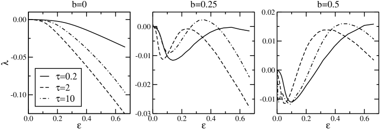
Figure 2: Samples of dependencies $\lambda(\varepsilon,\,\tau)$ for the Van der Pol–Duffing oscillator (10) at $\mu=0.1$. The values of the parameters $b$ and $\tau$ are indicated above the plots.

4 Conclusions

Having considered the phenomenon of synchronization of limit cycle oscillators by common telegraph noise, we can summarize:

— Either for weak noise or frequent switching the Lyapunov exponent is negative;

— For some systems, the phase model gives quite adequate results even for moderate noise levels and values of the average switching time;

— The dependence $\lambda(\varepsilon,\,\tau)$ for stochastic driving does not look to have any footprints of the one for periodic driving;

— In some systems, moderate telegraph noise can desynchronize oscillations.

Here we do not present results for the nonideal situations (like in Goldobin-Pikovsky-2005b ): slightly nonidentical oscillators driven by an identical noise signal, and identical oscillators driven by slightly nonidentical noise signals. The reason is that for weak noise these results appear to be the same as in Goldobin-Pikovsky-2005b but with $\lambda_{\mathrm{app}}$ given by Eq. (8) instead of $\lambda$.

References

- (1) R. L. Stratonovich, Topics in the Theory of Random Noise, Gordon and Breach, New York, 1963.
- (2) A. N. Malakhov, Fluctuations in Self–Oscillatory Systems, Nauka, Moscow, 1968, (In Russian).
- (3) A. S. Pikovsky, Radiophys. Quantum Electron. 27 (5), 576 (1984).
- (4) A. S. Pikovsky, ”Synchronization and stochastization of nonlinear oscillations by external noise”, in Nonlinear and Turbulent Processes in Physics, edited by R. Z. Sagdeev, Harwood Acad. Publ., Singapore, 1984, pp. 1601–1604.
- (5) A. S. Pikovsky, M. Rosenblum, and J. Kurths, Synchronization—A Unified Approach to Nonlinear Science, Cambridge University Press, Cambridge, UK, 2001.
- (6) L. Yu, E. Ott, and Q. Chen, Phys. Rev. Lett. 65, 2935 (1990).
- (7) L. Baroni, R. Livi, and A. Torcini, Phys. Rev. E 63, 036226 (2001).
- (8) P. Khoury, M. A. Lieberman, and A. J. Lichtenberg, Phys. Rev. E 54, 3377 (1996).
- (9) Z. F. Mainen and T. J. Sejnowski, Science 268, 1503 (1995).
- (10) A. Uchida, R. McAllister, and R. Roy, Phys. Rev. Lett. 93, 244102 (2004).
- (11) H. D. I. Abarbanel, N. F. Rulkov, and M. M. Suschik, Phys. Rev. E 53, 4528 (1996).
- (12) J. Teramae and D. Tanaka, Phys. Rev. Lett. 93, 204103 (2004)
- (13) D. S. Goldobin and A. S. Pikovsky, Phisica A 351, 126 (2005).
- (14) D. S. Goldobin and A. Pikovsky, Phys. Rev. E 71, 045201(R) (2005).
- (15) Y. Kuramoto, Chemical Oscillations, Waves and Turbulence, Dover, New York, 2003.