Bayesian Nonparametric Modeling for Multivariate Ordinal Regression

Abstract

Univariate or multivariate ordinal responses are often assumed to arise from a latent continuous parametric distribution, with covariate effects which enter linearly. We introduce a Bayesian nonparametric modeling approach for univariate and multivariate ordinal regression, which is based on mixture modeling for the joint distribution of latent responses and covariates. The modeling framework enables highly flexible inference for ordinal regression relationships, avoiding assumptions of linearity or additivity in the covariate effects. In standard parametric ordinal regression models, computational challenges arise from identifiability constraints and estimation of parameters requiring nonstandard inferential techniques. A key feature of the nonparametric model is that it achieves inferential flexibility, while avoiding these difficulties. In particular, we establish full support of the nonparametric mixture model under fixed cut-off points that relate through discretization the latent continuous responses with the ordinal responses. The practical utility of the modeling approach is illustrated through application to two data sets from econometrics, an example involving regression relationships for ozone concentration, and a multirater agreement problem. Supplementary materials related to computation are available online.

Keywords: Dirichlet process mixture model; Kullback-Leibler condition; Markov chain Monte Carlo; polychoric correlations.

1 Introduction

Estimating regression relationships for univariate or multivariate ordinal responses is a key problem in many application areas. Correlated ordinal data arise frequently in the social sciences, for instance, survey respondents often assign ratings on ordinal scales (such as “agree”, “neutral”, or “disagree”) to a set of questions, and the responses given by a single rater are correlated. Ordinal data is also commonly encountered in econometrics, as rating agencies (such as Standard and Poor’s) use an ordinal rating scale. A natural way to model data of this type is to envision each ordinal variable as representing a discretized version of an underlying latent continuous random variable. In particular, the commonly used (multivariate) ordinal probit model results when a (multivariate) normal distribution is assumed for the latent variable(s).

Under the probit model for a single ordinal response $Y$ with $C$ categories, and covariate vector $\boldsymbol{x}$, $\mathrm{Pr}(Y\leq m\mid\boldsymbol{x})=$ $\Phi(\gamma_{m}-\boldsymbol{x}^{T}\boldsymbol{\beta})$, for $m=1,\dots,C$. Here, $-\infty=\gamma_{0}<\gamma_{1}<\dots<\gamma_{C-1}<\gamma_{C}=\infty$ are cut-off points for the response categories, where typically $\gamma_{1}=0$ for identifiability. Albert and Chib (1993) have shown that posterior simulation is greatly simplified by augmenting the model with latent variables. In particular, assume that the ordinal response $Y$ arises from a latent continuous response $Z$, such that $Y=m$ if and only if $Z\in(\gamma_{m-1},\gamma_{m}]$, for $m=1,\dots,C$, and $Z\mid\boldsymbol{\beta}\sim\mathrm{N}(\boldsymbol{x}^{T}\boldsymbol{\beta},1)$, which yields $\mathrm{Pr}(Y=m\mid\boldsymbol{x})=$ $\int_{\gamma_{m-1}}^{\gamma_{m}}\mathrm{N}(z\mid\boldsymbol{x}^{T}\boldsymbol{\beta},1)\text{d}z$.

The multivariate probit model for binary or ordinal responses generalizes the probit model to accommodate correlated ordinal responses $\boldsymbol{Y}=$ $(Y_{1},...,Y_{k})$, where $Y_{j}\in$ $\{1,...,C_{j}\}$ for $j=1,...,k$, using a multivariate normal distribution for the underlying latent variables $\boldsymbol{Z}=$ $(Z_{1},...,Z_{k})$. To obtain an identifiable model, restrictions must be imposed on the covariance matrix $\boldsymbol{\Sigma}$ of the multivariate normal distribution for $\boldsymbol{Z}$. One way to handle this is to restrict the covariance matrix to be a correlation matrix, which complicates Bayesian inference since there does not exist a conjugate prior for correlation matrices. Chib and Greenberg (1998) discuss inference under this model, using a random walk Metropolis algorithm to sample the correlation matrix. Liu (2001) and Imai and van Dyk (2005) use parameter expansion with data augmentation (Liu and Wu, 1999) to expand the parameter space such that unrestricted covariance matrices may be sampled. Talhouk et al. (2012) work with a sparse correlation matrix arising from conditional independence assumptions, and use a parameter expansion strategy to expand the correlation matrix into a covariance matrix, which is updated with a Gibbs sampling step. Webb and Forster (2008) reparameterize $\boldsymbol{\Sigma}$ in a way that enables fixing its diagonal elements without sacrificing closed-form full conditional distributions. Lawrence et al. (2008) use a parameter expansion technique, in which the parameter space includes unrestricted covariance matrices, which are then normalized to correlation matrices. In addition to the challenges arising from working with correlation matrices, the setting with multivariate ordinal responses requires estimation for the cut-off points, which are typically highly correlated with the latent responses.

The assumption of normality on the latent variables is restrictive, especially for data which contains a large proportion of observations at high or low ordinal levels, and relatively few observations at moderate levels. As a consequence of the normal distribution shape, there are certain limitations on the effect that each covariate can have on the marginal probability response curves. In particular, $\mathrm{Pr}(Y_{j}=1\mid x)$ and $\mathrm{Pr}(Y_{j}=C_{j}\mid x)$ are monotonically increasing or decreasing as a function of covariate $x$, and they must have the opposite type of monotonicity. The direction of monotonicity changes exactly once in moving from category $1$ to $C_{j}$ (referred to as the single-crossing property). In addition, the relative effect of covariates $r$ and $s$, i.e., the ratio of $\partial\mathrm{Pr}(Y_{j}=m\mid\boldsymbol{x})/\partial x_{r}$ to $\partial\mathrm{Pr}(Y_{j}=m\mid\boldsymbol{x})/\partial x_{s}$, is equal to the ratio of the $r$-th and $s$-th regression coefficients for the $j$-th response, which does not depend on $m$ or $\boldsymbol{x}$. That is, the relative effect of one covariate to another is the same for every ordinal level and any covariate value. We refer to Boes and Winkelmann (2006) for further discussion of such properties.

Work on Bayesian nonparametric modeling for ordinal regression is relatively limited, particularly in the multivariate setting. In the special case of binary regression, there is only one probability response curve to be modeled, and this problem has received significant attention. Existing semiparametric approaches involve relaxing the normality assumption for the latent response (e.g., Newton et al., 1996; Basu and Mukhopadhyay, 2000), while others have targeted the linearity assumption for the response function (e.g., Mukhopadyay and Gelfand, 1997; Walker and Mallick, 1997; Choudhuri et al., 2007). For a univariate ordinal response, Chib and Greenberg (2010) assume that the latent response arises from scale mixtures of normals, and the covariate effects to be additive upon transformation by cubic splines. This allows nonlinearities to be obtained in the marginal regression curves, albeit under the restrictive assumption of additive covariate effects. Gill and Casella (2009) extend the ordinal probit model by introducing subject-specific random effects terms modeled with a Dirichlet process (DP) prior.

Chen and Dey (2000) model the latent variables for correlated ordinal responses with scale mixtures of normal distributions, with means linear on the covariates. Related, Bao and Hanson (2015) assume the latent variables arise from mixtures of linear multivariate probit regressions, mixing on the regression coefficients and covariance matrices in the multivariate normal distribution. The latter modeling approach is an extension of the work in Kottas et al. (2005), where, in the context of multivariate ordinal data without covariates, the latent response distribution was modeled with a DP mixture of multivariate normals. In the absence of covariates, this model is sufficiently flexible to uncover essentially any pattern in a contingency table while using fixed cut-offs. This represents a significant advantage relative to the parametric models discussed, since the estimation of cut-offs requires nonstandard inferential techniques, such as hybrid Markov chain Monte Carlo (MCMC) samplers (Johnson and Albert, 1999) and reparamaterization to achieve transformed cut-offs which do not have an order restriction (Chen and Dey, 2000).

The preceding discussion reflects the fact that there are significant challenges involved in fitting multivariate probit models, and a large amount of research has been dedicated to providing new inferential techniques in this setting. While the simplicity of its model structure and interpretability of its parameters make the probit model appealing to practitioners, the assumptions of linear covariate effects, and normality on the latent variables are restrictive. Hence, from both the methodological and practical point of view, it is important to explore more flexible modeling and inference techniques, especially for the setting with multivariate ordinal responses. Semiparametric methods for binary regression are more common, since in this case there is a single regression function to be modeled. When taken to the setting involving a single ordinal response with $C\geq 3$ classifications, it becomes much harder to incorporate flexible priors for each of the $C-1$ probability response curves. And, semiparametric prior specifications appear daunting in the multivariate ordinal regression setting where, in addition to general regression relationships, it is desirable to achieve flexible dependence structure between the ordinal responses.

Motivated by these limitations of parametric and semiparametric prior probability models, our goal is to develop a Bayesian nonparametric regression model for univariate and multivariate ordinal responses, which enables flexible inference for both the conditional response distribution and for regression relationships. We focus on problems where the covariates can be treated as random, and model the joint distribution of the covariates and latent responses with a DP mixture of multivariate normals to induce flexible regression relationships, as well as general dependence structure in the multivariate response distribution. In many fields – such as biometry, economics, and the environmental and social sciences – the assumption of random covariates is appropriate, indeed we argue necessary, as the covariates are not fixed prior to data collection.

In addition to the substantial distributional flexibility, an appealing aspect of the nonparametric modeling approach taken is that the cut-offs may be fixed, and the mixture kernel covariance matrix left unrestricted. Regarding the latter, we show that all parameters of the normal mixture kernel are identifiable provided each ordinal response comprises more than two classifications. For the former, we demonstrate that, with fixed cut-offs, our model can approximate arbitrarily well any set of probabilities on the ordinal outcomes. To this end, we prove that the induced prior on the space of mixed ordinal-continuous distributions assigns positive probability to all Kullback-Leibler (KL) neighborhoods of all densities in this space that satisfy certain regularity conditions.

We are primarily interested in regression relationships, and demonstrate that we can obtain inference for a variety of nonlinear as well as more standard shapes for ordinal regression curves, using data examples chosen from fields for which the methodology is particularly relevant. The joint response-covariate modeling approach yields more flexible inference for regression relationships than structured normal mixture models for the response distribution, such as the ones in Chen and Dey (2000) and Bao and Hanson (2015). Moreover, as a consequence of the joint modeling framework, inferences for the conditional covariate distribution given specific ordinal response categories, or inverse inferences, are also available. These relationships may be of direct interest in certain applications. Also of interest are the associations between the ordinal variables. These are described by the correlations between the latent variables in the ordinal probit model, termed polychoric correlations in the social sciences (e.g., Olsson, 1979). Using a data set of ratings assigned to essays by multiple raters, we apply our model to determine regions of the covariate space as well as the levels of ratings at which pairs of raters tend to agree or disagree. We contrast our approach with the Bayesian methods for studying multirater agreement in Johnson and Albert (1999) and Savitsky and Dalal (2014).

The work in this paper forms the sequel to DeYoreo and Kottas (2015), where we have developed the joint response-covariate modeling approach for binary regression, which requires use of more structured mixture kernels to satisfy necessary identifiability restrictions. The joint response-covariate modeling approach with categorical variables has been explored in a few other papers, including Shahbaba and Neal (2009), Dunson and Bhattacharya (2010), Hannah et al. (2011), and Papageorgiou et al. (2015). Shahbaba and Neal (2009) considered classification of a univariate response using a multinomial logit kernel, and this was extended by Hannah et al. (2011) to accommodate alternative response types with mixtures of generalized linear models. Dunson and Bhattacharya (2010) studied DP mixtures of independent kernels, and Papageorgiou et al. (2015) build a model for spatially indexed data of mixed type (count, categorical, and continuous). However, these models would not be suitable for ordinal data, or, particularly in the first three cases, when inferences are to be made on the association between ordinal response variables.

The rest of the article is organized as follows. In Section 2, we formulate the DP mixture model for ordinal regression, including study of the theoretical properties discussed above (with technical details given in the Appendix). We discuss prior specification and posterior inference, and indicate possible modifications when binary responses are present. The methodology is applied in Section 3 to ozone concentration data, two data examples from econometrics, and a multirater agreement problem. Finally, Section 4 concludes with a discussion.

2 Methodology

2.1 Model formulation

Suppose that $k$ ordinal categorical variables are recorded for each of $n$ individuals, along with $p$ continuous covariates, so that for individual $i$ we observe a response vector $\boldsymbol{y}_{i}=(y_{i1},\dots,y_{ik})$ and a covariate vector $\boldsymbol{x}_{i}=(x_{i1},\dots,x_{ip})$, with $y_{ij}\in\{1,\dots,C_{j}\}$, and $C_{j}>2$. Introduce latent continuous random variables $\boldsymbol{z}_{i}=(z_{i1},\dots,z_{ik})$, $i=1,\dots,n$, such that $y_{ij}=l$ if and only if $\gamma_{j,l-1}<z_{ij}\leq\gamma_{j,l}$, for $j=1,\dots,k$, and $l=1,\dots,C_{j}$. For example, in a biomedical application, $y_{i1}$ and $y_{i2}$ could represent severity of two different symptoms of patient $i$, recorded on a categorical scale ranging from “no problem” to “severe”, along with covariate information weight, age, and blood pressure. The assumption that the ordinal responses represent discretized versions of latent continuous responses is natural for many settings, such as the one considered here. Note also that the assumption of random covariates is appropriate in this application, and that the medical measurements are all related and arise from some joint stochastic mechanism. This motivates our focus on building a model for the joint density $f(\boldsymbol{z},\boldsymbol{x})$, which is a continuous density of dimension $k+p$, which in turn implies a model for the conditional response distribution $f(\boldsymbol{y}\mid\boldsymbol{x})$.

To model $f(\boldsymbol{z},\boldsymbol{x})$ in a flexible way, we use a DP mixture of multivariate normals model, mixing on the mean vector and covariance matrix. That is, we assume $(\boldsymbol{z}_{i},\boldsymbol{x}_{i})\mid G\stackrel{{\scriptstyle iid}}{{\sim}}\int\text{N}(\boldsymbol{z}_{i},\boldsymbol{x}_{i}\mid\boldsymbol{\mu},\boldsymbol{\Sigma})\text{d}G(\boldsymbol{\mu},\boldsymbol{\Sigma})$, and place a DP prior (Ferguson, 1973) on the random mixing distribution $G$. This DP mixture density regression approach was first proposed by Müller et al. (1996) in the context of continuous variables, and has been more recently studied under different modeling scenarios; see, e.g., Müller and Quintana (2010), Park and Dunson (2010), Taddy and Kottas (2010), Taddy and Kottas (2012), and Wade et al. (2014). Norets and Pelenis (2012) established large support and other theoretical properties for conditional distributions that are induced from finite mixtures of multivariate normals, where the response and covariates may be either discrete or continuous variables.

The hierarchical model is formulated by introducing a latent mixing parameter $\boldsymbol{\theta_{i}}=(\boldsymbol{\mu}_{i},\boldsymbol{\Sigma}_{i})$ for each data vector:

$$(\boldsymbol{z}_{i},\boldsymbol{x}_{i})\mid\boldsymbol{\theta}_{i}\stackrel{{\scriptstyle ind.}}{{\sim}}\text{N}(\boldsymbol{\mu}_{i},\boldsymbol{\Sigma}_{i});\,\,\,\,\,\boldsymbol{\theta}_{i}\mid G\stackrel{{\scriptstyle iid}}{{\sim}}G,\quad i=1,\dots,n$$ (1)

where $G\mid\alpha,\boldsymbol{\psi}\sim\text{DP}(\alpha,G_{0}(\cdot\mid\boldsymbol{\psi}))$, with base (centering) distribution $G_{0}(\boldsymbol{\mu},\boldsymbol{\Sigma}\mid\boldsymbol{\psi})=$ $\text{N}(\boldsymbol{\mu}\mid\boldsymbol{m},\boldsymbol{V})\text{IW}(\boldsymbol{\Sigma}\mid\nu,\boldsymbol{S})$. The model is completed with hyperpriors on $\boldsymbol{\psi}=$ $(\boldsymbol{m},\boldsymbol{V},\boldsymbol{S})$, and a prior on $\alpha$:

$$\boldsymbol{m}\sim\text{N}(\boldsymbol{a}_{\boldsymbol{m}},\boldsymbol{B}_{\boldsymbol{m}}),\quad\boldsymbol{V}\sim\text{IW}(a_{\boldsymbol{V}},\boldsymbol{B}_{\boldsymbol{V}}),\quad\boldsymbol{S}\sim\text{W}(a_{\boldsymbol{S}},\boldsymbol{B}_{\boldsymbol{S}}),\quad\alpha\sim\text{gamma}(a_{\alpha},b_{\alpha}),$$ (2)

where W$(a_{\boldsymbol{S}},\boldsymbol{B}_{\boldsymbol{S}})$ denotes a Wishart distribution with mean $a_{\boldsymbol{S}}\boldsymbol{B}_{\boldsymbol{S}}$, and IW$(a_{\boldsymbol{V}},\boldsymbol{B}_{\boldsymbol{V}})$ denotes an inverse-Wishart distribution with mean $(a_{\boldsymbol{V}}-(k+p)-1)^{-1}\boldsymbol{B}_{\boldsymbol{V}}$.

According to its constructive definition (Sethuraman, 1994), the DP generates almost surely discrete distributions, $G=\sum_{l=1}^{\infty}p_{l}\delta_{\boldsymbol{\vartheta}_{l}}$. The atoms ${\boldsymbol{\vartheta}}_{l}$ are independent realizations from $G_{0}$, and the weights are determined through stick-breaking from beta distributed random variables with parameters 1 and $\alpha$. That is, $p_{1}=v_{1}$, and $p_{l}=v_{l}\prod_{r=1}^{l-1}(1-v_{r})$, for $l=2,3,\dots$, with $v_{l}\stackrel{{\scriptstyle iid}}{{\sim}}\text{beta}(1,\alpha)$. The discreteness of the DP allows for ties in the $\boldsymbol{\theta}_{i}$, so that in practice less than $n$ distinct values for the $\{\boldsymbol{\theta}_{i}\}$ are imputed. The data is therefore clustered into a typically small number of groups relative to $n$, with the number of clusters $n^{*}$ controlled by parameter $\alpha$, where larger values favor more clusters (Escobar and West, 1995). From the constructive definition for $G$, the prior model for $f(\boldsymbol{z},\boldsymbol{x})$ has an almost sure representation as a countable mixture of multivariate normals, and the proposed model can therefore be viewed as a nonparametric extension of the multivariate probit model, albeit with random covariates.

This implies a countable mixture of normal distributions (with covariate-dependent weights) for $f(\boldsymbol{z}\mid\boldsymbol{x},G)$, from which the latent $\boldsymbol{z}$ may be integrated out to reveal the induced model for the ordinal regression relationships. In general, for a multivariate response $\boldsymbol{Y}=(Y_{1},\dots,Y_{k})$ with an associated covariate vector $\boldsymbol{X}$, the probability that $\boldsymbol{Y}$ takes on the values $\boldsymbol{l}=(l_{1},\dots,l_{k})$, where $l_{j}\in\{1,\dots,C_{j}\}$, for $j=1,\dots,k$, can be expressed as

$$\mathrm{Pr}(\boldsymbol{Y}=\boldsymbol{l}\mid\boldsymbol{x},G)=\sum_{r=1}^{\infty}w_{r}(\boldsymbol{x})\int_{\gamma_{k,l_{k}-1}}^{\gamma_{k,l_{k}}}\cdot\cdot\cdot\int_{\gamma_{1,l_{1}-1}}^{\gamma_{1,l_{1}}}\text{N}(\boldsymbol{z}\mid\boldsymbol{m}_{r}(\boldsymbol{x}),\boldsymbol{S}_{r})\text{d}\boldsymbol{z}$$ (3)

with covariate-dependent weights $w_{r}(\boldsymbol{x})\propto p_{r}\text{N}(\boldsymbol{x}\mid\boldsymbol{\mu}_{r}^{x},\boldsymbol{\Sigma}_{r}^{xx})$, and mean vectors $\boldsymbol{m}_{r}(\boldsymbol{x})=\boldsymbol{\mu}_{r}^{z}+\boldsymbol{\Sigma}_{r}^{zx}(\boldsymbol{\Sigma}_{r}^{xx})^{-1}(\boldsymbol{x}-\boldsymbol{\mu}_{r}^{x})$, and covariance matrices $\boldsymbol{S}_{r}=\boldsymbol{\Sigma}_{r}^{zz}-\boldsymbol{\Sigma}_{r}^{zx}(\boldsymbol{\Sigma}_{r}^{xx})^{-1}\boldsymbol{\Sigma}_{r}^{xz}$. Here, $(\boldsymbol{\mu}_{r},\boldsymbol{\Sigma}_{r})$ are the atoms in the DP prior constructive definition, where $\boldsymbol{\mu}_{r}$ is partitioned into $\boldsymbol{\mu}_{r}^{z}$ and $\boldsymbol{\mu}_{r}^{x}$ according to random vectors $\boldsymbol{Z}$ and $\boldsymbol{X}$, and $(\boldsymbol{\Sigma}_{r}^{zz},\boldsymbol{\Sigma}_{r}^{xx},\boldsymbol{\Sigma}_{r}^{zx},\boldsymbol{\Sigma}_{r}^{xz})$ are the components of the corresponding partition of covariance matrix $\boldsymbol{\Sigma}_{r}$.

To illustrate, consider a bivariate response $\boldsymbol{Y}=(Y_{1},Y_{2})$, with covariates $\boldsymbol{X}$. The probability assigned to the event $(Y_{1}=l_{1})\cap(Y_{2}=l_{2})$ is obtained using (3), which involves evaluating bivariate normal distribution functions. However, one may be interested in the marginal relationships between individual components of $\boldsymbol{Y}$ and the covariates. Referring to the example given at the start of this section, we may obtain the probability that both symptoms are severe as a function of $\boldsymbol{X}$, but also how the first varies as a function of $\boldsymbol{X}$. The marginal inference, $\mathrm{Pr}(Y_{1}=l_{1}\mid\boldsymbol{x},G)$, is given by the expression

$$\sum_{r=1}^{\infty}w_{r}(\boldsymbol{x})\left\{\Phi\left(\frac{\gamma_{1,l_{1}}-m_{r}(\boldsymbol{x})}{s_{r}^{1/2}}\right)-\Phi\left(\frac{\gamma_{1,l_{1}-1}-m_{r}(\boldsymbol{x})}{s_{r}^{1/2}}\right)\right\}$$ (4)

where $m_{r}(\boldsymbol{x})$ and $s_{r}$ are the conditional mean and variance for $z_{1}$ conditional on $\boldsymbol{x}$ implied by the joint distribution $\mathrm{N}(\boldsymbol{z},\boldsymbol{x}\mid\boldsymbol{\mu}_{r},\boldsymbol{\Sigma}_{r})$. Expression (4) provides also the form of the ordinal regression curves in the case of a single response.

Hence, the implied regression relationships have a mixture structure with component-specific kernels which take the form of parametric probit regressions, and weights which are covariate-dependent. This structure enables inference for non-linear response curves, by favoring a set of parametric models with varying probabilities depending on the location in the covariate space. The limitations of parametric probit models – including relative covariate effects which are constant in terms of the covariate and the ordinal level, monotonicity, and the single-crossing property of the response curves – are thereby overcome.

2.2 Model properties

In (1), $\boldsymbol{\Sigma}$ was left an unrestricted covariance matrix. As an alternative to working with correlation matrices under the probit model, identifiability can be achieved by fixing $\gamma_{j,2}$ (in addition to $\gamma_{j,1}$), for $j=1,\dots,k$. As shown here, analogous results can be obtained in the random covariate setting. In particular, Lemma 1 establishes identifiability for $\boldsymbol{\Sigma}$ as a general covariance matrix in a parametric ordered probit model with random covariates, assuming all cut-offs, $\gamma_{j,1},\dots,\gamma_{j,C_{j}-1}$, for $j=1,\dots,k$, are fixed. Here, model identifiability refers to likelihood identifiability of the mixture kernel parameters in the induced model for $(\boldsymbol{Y},\boldsymbol{X})$ under a single mixture component.

Lemma 1. Consider a multivariate normal model, $\text{N}(\boldsymbol{Z},\boldsymbol{X}\mid\boldsymbol{\mu},\boldsymbol{\Sigma})$, for the joint distribution of latent responses $\boldsymbol{Z}$ and covariates $\boldsymbol{X}$, with fixed cut-off points defining the ordinal responses $\boldsymbol{Y}$ through $\boldsymbol{Z}$. Then, the parameters $\boldsymbol{\mu}$ and $\boldsymbol{\Sigma}$ are identifiable in the implied model for $(\boldsymbol{Y},\boldsymbol{X})$, and therefore in the kernel of the implied mixture model for $(\boldsymbol{Y},\boldsymbol{X})$, provided $C_{j}>2$, for $j=1,\dots,k$.

Refer to Appendix A for a proof of this result. If $C_{j}=2$ for some $j$, additional restrictions are needed for identifiability, as discussed in Section 2.5.

We emphasize that Lemma 1 does not imply that the parameters of the mixture model are identifiable, rather it establishes identifiability for the kernel of the mixture model. Identifiability is a basic model property for parametric probit models (Hobert and Casella, 1996; McCulloch et al., 2000; Koop, 2003; Talhouk et al., 2012), and is achieved for the special one-component case of our model, a multivariate ordered probit model with random covariates, by fixing the cut-offs. However, this may appear to be a significant restriction, as under the parametric probit setting, fixing all cut-off points would prohibit the model from being able to adequately assign probabilities to the regions determined by the cut-offs. We therefore seek to determine if the nonparametric model with fixed cut-offs is sufficiently flexible to accommodate general distributions for $(\boldsymbol{Y},\boldsymbol{X})$ and also for $\boldsymbol{Y}\mid\boldsymbol{X}$. Kottas et al. (2005) provide an informal argument that the normal DP mixture model for multivariate ordinal responses (without covariates) can approximate arbitrarily well any probability distribution for a contingency table. The basis for this argument is that, in the limit, one mixture component can be placed within each set of cut-offs corresponding to a specific ordinal vector, with the mixture weights assigned accordingly to each cell.

Here, we provide a proof of the full support of our more general model for ordinal-continuous distributions. In addition to being a desirable property on its own, the ramifications of full support for the prior model are significant, as it is a key condition for the study of posterior consistency (e.g., Ghosh and Ramamoorthi, 2003). Using the KL divergence to define density neighborhoods, a particular density $f_{0}$ is in the KL support of the prior $\mathcal{P}$, if $\mathcal{P}(K_{\epsilon}(f_{0}))>0$, for any $\epsilon>0$, where $K_{\epsilon}(f_{0})=$ $\{f:\int f_{0}(\boldsymbol{w})\log(f_{0}(\boldsymbol{w})/f(\boldsymbol{w}))\text{d}\boldsymbol{w}<\epsilon\}$. The KL property is satisfied if any density (typically subject to regularity conditions) in the space of interest is in the KL support of the prior.

It has been established that the DP location normal mixture prior model satisfies the KL property (Wu and Ghosal, 2008). That is, if the mixing distribution $G$ is assigned a DP prior on the space of random distributions for $\boldsymbol{\mu}$, and a normal kernel is chosen such that $f(\boldsymbol{w}\mid G,\boldsymbol{\Sigma})=$ $\int\mathrm{N}(\boldsymbol{w}\mid\boldsymbol{\mu},\boldsymbol{\Sigma})dG(\boldsymbol{\mu})$, with $\boldsymbol{\Sigma}$ a diagonal matrix, then the induced prior model for densities has full KL support. Letting this induced prior be denoted by $\mathcal{P}$, and modeling the joint distribution of $(\boldsymbol{X},\boldsymbol{Z})$ with a DP location mixture of normals, the KL property yields:

$$\mathcal{P}\left(\{f:\int f_{0}(\boldsymbol{x},\boldsymbol{z})\log(f_{0}(\boldsymbol{x},\boldsymbol{z})/f(\boldsymbol{x},\boldsymbol{z}))\text{d}\boldsymbol{x}\text{d}\boldsymbol{z}<\epsilon\}\right)>0,\,\,\,\,\,\text{for any}\,\,\,\epsilon>0$$ (5)

for all densities $f_{0}(\boldsymbol{x},\boldsymbol{z})$ on $\mathbb{R}^{p+k}$ that satisfy certain regularity conditions.

To establish the KL property of the prior on mixed ordinal-continuous distributions for $(\boldsymbol{X},\boldsymbol{Y})$ induced from multivariate continuous distributions for $(\boldsymbol{X},\boldsymbol{Z})$, consider a generic data-generating distribution $p_{0}(\boldsymbol{x},\boldsymbol{y})\in\mathcal{D^{*}}$. Here, $\mathcal{D^{*}}$ denotes the space of distributions on $\mathbb{R}^{p}\times\{1,\dots,C_{1}\}\times\cdot\cdot\cdot\times\{1,\dots,C_{k}\}$. Let $f_{0}(\boldsymbol{x},\boldsymbol{z})\in\mathcal{D}$, where $\mathcal{D}$ denotes the space of densities on $\mathbb{R}^{p+k}$, such that

$$p_{0}(\boldsymbol{x},l_{1},\dots,l_{k})=\int_{\gamma_{k,l_{k}-1}}^{\gamma_{k,l_{k}}}\cdot\cdot\cdot\int_{\gamma_{1,l_{1}-1}}^{\gamma_{1,l_{1}}}f_{0}(\boldsymbol{x},z_{1},\dots,z_{k})\,\text{d}z_{1}\cdot\cdot\cdot\text{d}z_{k}$$ (6)

for any $(l_{1},...,l_{k})$, where $l_{j}\in\{1,\dots,C_{j}\}$, for $j=1,\dots,k$. That is, $f_{0}(\boldsymbol{x},\boldsymbol{z})$ is the density of a latent continuous distribution which induces the corresponding distribution on the ordinal responses. Note that at least one $f_{0}\in\mathcal{D}$ exists for each $p_{0}\in\mathcal{D^{*}}$, with one such $f_{0}$ described in Appendix B2.

The next lemma (proved in Appendix B1) establishes that, as a consequence of the KL property of the DP mixture of normals (5), the prior assigns positive probability to all KL neighborhoods of $p_{0}(\boldsymbol{x},\boldsymbol{y})$, as well as to all KL neighborhoods of the implied conditional distributions $p_{0}(\boldsymbol{y}\mid\boldsymbol{x})$. We prove the lemma assuming that $p_{0}$ satisfies generic regularity conditions such that the corresponding $f_{0}$ is in the KL support of the prior. Hence, the result may be useful for other prior model settings for the latent continuous distribution $f(\boldsymbol{z},\boldsymbol{x})$. Lemma 2 extends to the regression setting analogous KL support results for discrete and mixed discrete-continuous distributions (Canale and Dunson, 2011, 2015). To ensure the KL property is satisfied for the proposed model, we also include in Appendix B2 a set of conditions for $p_{0}$ under which a specific corresponding $f_{0}$ satisfies (5), in particular, it satisfies the general conditions for the KL property given in Theorem 2 of Wu and Ghosal (2008).

Lemma 2. Assume that the distribution of a mixed ordinal-continuous random variable, $p_{0}(\boldsymbol{x},\boldsymbol{y})\in\mathcal{D^{*}}$, satisfies appropriate regularity conditions such that for the corresponding density, $f_{0}(\boldsymbol{x},\boldsymbol{z})\in\mathcal{D}$, we have $\mathcal{P}(K_{\epsilon}(f_{0}(\boldsymbol{x},\boldsymbol{z})))>0$, for any $\epsilon>0$. Then, $\mathcal{P}(K_{\epsilon}(p_{0}(\boldsymbol{x},\boldsymbol{y})))>0$ and $\mathcal{P}(K_{\epsilon}(p_{0}(\boldsymbol{y}\mid\boldsymbol{x})))>0$, for any $\epsilon>0$.

Lemma 2 establishes full KL support for a model arising from a DP location normal mixture, a simpler version of our model. The KL property reflects a major advantage of the proposed modeling approach in that it offers flexible inference for multivariate ordinal regression while avoiding the need to impute cut-off points, which is a major challenge in fitting multivariate probit models.

The cut-off points can be fixed to arbitrary increasing values, which, for instance, may be equally spaced and centered at zero. As confirmed empirically with simulated data (refer to Section 3 for details), the choice of cut-offs does not affect inferences for the ordinal regression relationships, only the center and scale of the latent variables, which must be interpreted relative to the cut-offs.

2.3 Prior specification

To implement the model, we need to specify the parameters of the hyperpriors in (2). A default specification strategy is developed by considering the limiting case of the model as $\alpha\rightarrow 0^{+}$, which results in a single normal distribution for $(\boldsymbol{Z},\boldsymbol{X})$. This limiting model is essentially the multivariate probit model, with the addition of random covariates. The only covariate information we use here is an approximate center and range for each covariate, denoted by $\boldsymbol{c}^{x}=$ $(c_{1}^{x},\dots,c_{p}^{x})$ and $\boldsymbol{r}^{x}=$ $(r_{1}^{x},\dots,r_{p}^{x})$. Then $c_{m}^{x}$ and $r_{m}^{x}/4$ are used as proxies for the marginal mean and standard deviation of $X_{m}$. We also seek to center and scale the latent variables appropriately, using the cut-offs. Since $Y_{j}$ is supported on $\{1,\dots,C_{j}\}$, latent continuous variable $Z_{j}$ must be supported on values slightly below $\gamma_{j,1}$, up to slightly above $\gamma_{j,C_{j}-1}$. We therefore use $r_{j}^{z}/4$, where $r_{j}^{z}=(\gamma_{j,C_{j}-1}-\gamma_{j,1})$, as a proxy for the standard deviation of $Z_{j}$.

Under $(\boldsymbol{Z},\boldsymbol{X})\mid\boldsymbol{\mu},\boldsymbol{\Sigma}\sim\text{N}(\boldsymbol{\mu},\boldsymbol{\Sigma})$, we have $\text{E}(\boldsymbol{Z},\boldsymbol{X})=$ $\boldsymbol{a_{m}}$, and $\text{Cov}(\boldsymbol{Z},\boldsymbol{X})=$ $a_{\boldsymbol{S}}\boldsymbol{B}_{\boldsymbol{S}}(\nu-d-1)^{-1}$ + $\boldsymbol{B}_{\boldsymbol{V}}(a_{\boldsymbol{V}}-d-1)^{-1}$ + $\boldsymbol{B}_{\boldsymbol{m}}$, with $d=p+k$. Then, assuming each set of cut-offs $(\gamma_{j,0},\dots,\gamma_{j,C_{j}})$ are centered at 0, we fix $a_{m}=(0,\dots,0,\boldsymbol{c}^{x})$. Letting $\boldsymbol{D}=$ $\text{diag}\{(r_{1}^{{z}}/4)^{2},\dots,(r_{k}^{{z}}/4)^{2},(r_{1}^{{x}}/4)^{2},\dots,(r_{p}^{{x}}/4)^{2}\}$, each of the three terms in $\text{Cov}(\boldsymbol{Z},\boldsymbol{X})$ can be assigned an equal proportion of the total covariance, and set to $(1/3)\boldsymbol{D}$, or to $(1/2)\boldsymbol{D}$ to inflate the variance slightly. For dispersed but proper priors with finite expectation, $\nu$, $a_{\boldsymbol{V}}$, and $a_{\boldsymbol{S}}$ can be fixed to $d+2$. Fixing these parameters allows for $\boldsymbol{B_{S}}$ and $\boldsymbol{B_{V}}$ to be determined accordingly, completing the default specification strategy for the hyperpriors of $\boldsymbol{m}$, $\boldsymbol{V}$, and $\boldsymbol{S}$.

In the strategy outlined above, the form of $\text{Cov}(\boldsymbol{Z},\boldsymbol{X})$ was diagonal, such that a priori we favor independence between $\boldsymbol{Z}$ and $\boldsymbol{X}$ within a particular mixture component. Combined with the other aspects of the prior specification approach, this generally leads to prior means for the ordinal regression curves which do not have any trend across the covariate space. Moreover, the corresponding prior uncertainty bands span a significant portion of the unit interval.

2.4 Posterior inference

There exist many MCMC algorithms for DP mixtures, including marginal samplers (e.g., Neal, 2000), slice sampling algorithms (e.g., Kalli et al., 2011), and methods that involve truncation of the mixing distribution $G$ (e.g., Ishwaran and James, 2001). If the inference objectives are limited to posterior predictive estimation, which does not require posterior samples for $G$, the former two options may be preferable since they avoid truncation of $G$. However, under the joint modeling approach for the response-covariate distribution, posterior simulation must be extended to $G$ to obtain full inference for regression functionals, and this requires truncation regardless of the chosen MCMC approach. Since our contribution is on flexible mixture modeling for ordinal regression, we view the choice of the posterior simulation method as one that should balance efficiency with ease of implementation.

The MCMC posterior simulation method we utilize is based on a finite truncation approximation to the countable mixing distribution $G$, using the DP stick-breaking representation. The blocked Gibbs sampler (Ishwaran and Zarepour, 2000; Ishwaran and James, 2001) replaces the countable sum with a finite sum, $G_{N}=$ $\sum_{l=1}^{N}p_{l}\delta_{(\boldsymbol{\mu}_{l},\boldsymbol{\Sigma}_{l})}$, with $(\boldsymbol{\mu}_{l},\boldsymbol{\Sigma}_{l})$ i.i.d. from $G_{0}$, for $l=1,...,N$. Here, the first $N-1$ elements of $\boldsymbol{p}=$ $(p_{1},...,p_{N})$ are equivalent to those in the countable representation of $G$, whereas $p_{N}=$ $1-\sum_{l=1}^{N-1}p_{l}$. Under this approach, the posterior samples for model parameters yield posterior samples for $G_{N}$, and therefore full inference is available for mixture functionals.

The truncation level $N$ can be chosen to any desired level of accuracy, using standard DP properties. In particular, the expectation for the partial sum of the original DP weights, $\mathrm{E}(\sum\nolimits_{l=1}^{N}p_{l}\mid\alpha)=$ $1-\{\alpha/(\alpha+1)\}^{N}$, can be averaged over the prior for $\alpha$ to estimate the marginal prior expectation, $\mathrm{E}(\sum\nolimits_{l=1}^{N}p_{l})$, which is then used to specify $N$ given a tolerance level for the approximation. For instance, for the data example of Section 3.1, we set $N=50$, which under a $\mathrm{gamma}(0.5,0.5)$ prior for $\alpha$, yields $\mathrm{E}(\sum\nolimits_{l=1}^{50}p_{l})\approx 0.99994$.

To express the hierarchical model for the data after replacing $G$ with $G_{N}$, introduce configuration variables $(L_{1},\dots,L_{n})$, such that $L_{i}=l$ if and only if $\boldsymbol{\theta}_{i}=$ $(\boldsymbol{\mu}_{l},\boldsymbol{\Sigma}_{l})$, for $i=1,...,n$ and $l=1,...,N$. Then, the model for the data becomes

$$y_{ij}=l\quad\mathrm{iff}\quad\gamma_{j,l-1}<z_{ij}\leq\gamma_{j,l},\quad i=1,\dots,n,\quad j=1,\dots,k$$

$$(\boldsymbol{z}_{i},\boldsymbol{x}_{i})\mid\{(\boldsymbol{\mu}_{l},\boldsymbol{\Sigma}_{l}):l=1,...,N\},L_{i}\stackrel{{\scriptstyle ind.}}{{\sim}}\text{N}(\boldsymbol{\mu}_{L_{i}},\boldsymbol{\Sigma}_{L_{i}}),\quad i=1,\dots,n$$

$$L_{i}\mid\boldsymbol{p}\stackrel{{\scriptstyle iid}}{{\sim}}\sum\nolimits_{l=1}^{N}p_{l}\delta_{l}(L_{i}),\quad i=1,...,n$$

$$(\boldsymbol{\mu}_{l},\boldsymbol{\Sigma}_{l})\mid\boldsymbol{\psi}\stackrel{{\scriptstyle iid}}{{\sim}}\text{N}(\boldsymbol{\mu}_{l}\mid\boldsymbol{m},\boldsymbol{V})\text{IW}(\boldsymbol{\Sigma}_{l}\mid\nu,\boldsymbol{S}),\quad l=1,\dots,N$$

where the prior density for $\boldsymbol{p}$ is given by $\alpha^{N-1}p_{N}^{\alpha-1}(1-p_{1})^{-1}(1-(p_{1}+p_{2}))^{-1}\times\dots\times(1-\sum\nolimits_{l=1}^{N-2}p_{l})^{-1}$, which is a special case of the generalized Dirichlet distribution. The full model is completed with the conditionally conjugate priors on $\boldsymbol{\psi}$ and $\alpha$ as given in (2).

All full posterior conditional distributions are readily sampled, enabling efficient Gibbs sampling from the joint posterior distribution of the model above. Conditional on the latent responses $\boldsymbol{z}_{i}$, we have standard updates for the parameters of a normal DP mixture model. And conditional on the mixture model parameters, each $z_{ij}$, for $i=1,\dots,n$ and $j=1,\dots,k$, has a truncated normal full conditional distribution supported on the interval $(\gamma_{j,y_{ij}-1},\gamma_{j,y_{ij}}]$.

The regression functional $\mathrm{Pr}(\boldsymbol{Y}=\boldsymbol{l}\mid\boldsymbol{x},G)$ (estimated by the truncated version of (3) implied by $G_{N}$) can be computed over a grid in $\boldsymbol{x}$ at every MCMC iteration. This yields an entire set of samples for ordinal response probabilities at any covariate value $\boldsymbol{x}$ (note that $\boldsymbol{x}$ may include just a portion of the covariate vector or a single covariate). As indicated in (4), in the multivariate setting, we may wish to report inference for individual components of $\boldsymbol{Y}$ over the covariate space.

In some applications, in addition to modeling how $\boldsymbol{Y}$ varies across $\boldsymbol{X}$, we may also be interested in how the distribution of $\boldsymbol{X}$ changes at different ordinal values of $\boldsymbol{Y}$. As a feature of the modeling approach, we can obtain inference for $f(\boldsymbol{x}\mid\boldsymbol{y},G)$, for any configuration of ordinal response levels $\boldsymbol{y}$. We refer to these inferences as inverse relationships, and illustrate them with the data example of Section 3.2.

Under the multivariate response setting, the association between the ordinal variables may also be a key target of inference. In the social sciences, the correlations between pairs of latent responses, $\text{corr}(Z_{r},Z_{s})$, are termed polychoric correlations (Olsson, 1979) when a single multivariate normal distribution is used for the latent responses. Under our mixture modeling framework, we can sample a single $\text{corr}(Z_{r},Z_{s})$ at each MCMC iteration according to the corresponding $\boldsymbol{p}$, providing posterior predictive inference to assess overall agreement between pairs of response variables. As an alternative, and arguably more informative measure of association, we can obtain inference for probability of agreement over each covariate, or probability of agreement at each ordinal level. These inferences can be used to identify parts of the covariate space where there is agreement between response variables, as well as the ordinal values which are associated with higher levels of agreement. In the social sciences it is common to assess agreement among multiple raters or judges who are assigning a grade to the same item. In Section 3.4, we illustrate our methods with such a multirater agreement data example, in which both estimating regression relationships and modeling agreement are major objectives.

2.5 Accommodating binary responses

Our methodology focuses on multivariate ordinal responses with $C_{j}>2$, for all $j$. However, if one or more responses is binary, then the full covariance matrix of the normal mixture kernel for $(\boldsymbol{Z},\boldsymbol{X})$ is not identifiable. In the univariate probit model, it is standard practice to assume that $Z\mid\boldsymbol{\beta}\sim$ $\mathrm{N}(\boldsymbol{x}^{T}\boldsymbol{\beta},1)$, that is, identifiability is achieved by fixing $\Sigma^{zz}$. DeYoreo and Kottas (2015) show that a similar restriction can be used to facilitate identifiability in the binary probit model with random covariates, which is built from a multivariate normal distribution for the single latent response and covariates.

Under the general setting involving some binary and some ordinal responses, extending the argument that led to Lemma 1, it can be shown that identifiability is accomplished by fixing the diagonal elements of $\boldsymbol{\Sigma}^{zz}$ that correspond to the variances of the latent binary responses (the associated covariance elements remain identifiable). To incorporate this restriction, the inverse Wishart distribution for the component of $G_{0}$ that corresponds to $\boldsymbol{\Sigma}$ must be replaced with a more structured specification. To this end, a square-root-free Cholesky decomposition of $\boldsymbol{\Sigma}$ (Daniels and Pourahmadi, 2002; Webb and Forster, 2008) can be used to fix $\Sigma^{zz}$ in the setting with a single binary response (DeYoreo and Kottas, 2015), and this is also useful in the multivariate setting. This decomposition expresses $\boldsymbol{\Sigma}$ in terms of a unit lower triangular matrix $\boldsymbol{B}$, and a diagonal matrix $\boldsymbol{\Delta}$, with elements $\delta_{i}>0$, $i=1,...,k+p$, such that $\boldsymbol{\Sigma}=$ $\boldsymbol{B}^{-1}\boldsymbol{\Delta}(\boldsymbol{B}^{-1})^{T}$. The key result is that if $(W_{1},\dots,W_{r})\sim$ $\mathrm{N}(\boldsymbol{\mu},\boldsymbol{B}^{-1}\boldsymbol{\Delta}(\boldsymbol{B}^{-1})^{T})$, then this implies $\text{Var}(W_{i}\mid W_{1},\dots,W_{i-1})=$ $\delta_{i}$, for $i=2,\dots,r$. Therefore, if $(\boldsymbol{Z},\boldsymbol{X})\sim$ $\mathrm{N}(\boldsymbol{\mu},\boldsymbol{B}^{-1}\boldsymbol{\Delta}(\boldsymbol{B}^{-1})^{T})$, with $(Z_{1},\dots,Z_{r})$ binary, and $(Z_{r+1},\dots,Z_{k})$ ordinal, then fixing $\delta_{1}$ fixes $\text{Var}(Z_{1})$, fixing $\delta_{2}$ fixes $\text{Var}(Z_{2}\mid Z_{1})$, and so on. The scale of the latent binary responses may therefore be constrained by fixing $\delta_{1}$, the variance of the first latent binary response, $Z_{1}$, and the conditional variances $(\delta_{2},\dots,\delta_{r})$ of the remaining latent binary responses $(Z_{2},\dots,Z_{r})$. The conditional variances $(\delta_{r+1},\dots,\delta_{k+p})$ are not restricted, since they correspond to the scale of latent ordinal responses or covariates, which are identifiable under our model with fixed cut-offs.

The restricted version of the model for binary responses may be appealing because it implies that the special case of the mixture model consisting of a single mixture component (the parametric probit model) is identifiable. There is some empirical evidence from the literature that forcing the mixture kernel to be identifiable can improve MCMC performance (e.g., Di Lucca et al., 2013; DeYoreo and Kottas, 2015). To establish full support for the restricted prior model, the result of Lemma 2 would need to be extended, since the prior mixture model for the latent continuous distribution is modified. Alternatively, with sufficient care in MCMC implementation, the mixture model with the unrestricted kernel covariance matrix can be applied with binary responses. Note that Lemma 2 does not require the $C_{j}>2$ assumption, that is, it is applicable to settings with a combination of binary and more general ordinal responses.

3 Data Examples

The model was extensively tested on simulated data, where the primary goal was to assess how well it can estimate regression functionals which exhibit highly non-linear trends. We also explored effects of sample size, choice of cut-offs, and number of response categories. Some results from simulation studies are presented in the supplementary material.

The effect of sample size was observed in the uncertainty bands for the regression functions, which were reduced in width and became smoother with a larger sample size. The regression estimates captured the truth well in all cases, but were smoother and more accurate with more data, as expected. Even with a five-category ordinal response and only $200$ observations, the model was able to capture quite well non-standard regression curves.

As discussed previously, the cut-offs may be fixed to arbitrary increasing values, with the choice expected to have no impact on inference involving the relationship between $\boldsymbol{Y}$ and $\boldsymbol{X}$. To test this point, the model was fit to a synthetic data set containing an ordinal response with three categories, using cut-off points of $(-\infty,-20,20,\infty)$ and $(-\infty,-5,5,\infty)$, as well as cut-offs $(-\infty,0,0.1,\infty)$, which correspond to a narrow range of latent $Z$ values producing response value $Y=2$. The ordinal regression function estimates were unaffected by the change in cut-offs. The last set of cut-offs forces the model to generate components with small variance (lying in the interval $(0,0.1)$), but the resulting regression estimates are unchanged from the previous ones.

In the data illustrations that follow, the default prior specification strategy outlined in Section 2.3 was used. The posterior distributions for each component of $\boldsymbol{m}$ were always very peaked compared to the prior. Some sensitivity to the priors was found in terms of posterior learning for hyperparameters $\boldsymbol{V}$ and $\boldsymbol{S}$, however this was not reflected in the posterior inferences for the regression functions, which displayed little to no change when the priors were altered. Regarding the DP precision parameter $\alpha$, we noticed a moderate amount of learning for larger data sets, and a small amount for smaller data sets, which is consistent with what has been empirically observed about $\alpha$ in DP mixtures. The prior for $\alpha$ was in all cases chosen to favor reasonably large values, relative to the sample size, for the number of distinct mixture components.

In all data examples, a total of at least 100,000 MCMC samples were taken. The first 5,000 to 10,000 were discarded as burn in, and the remaining draws were thinned to reduce autocorrelation. The models were programmed in R and run on a desktop computer with Intel 3.4 GHz. To provide an idea of how long the algorithm takes to run, for the ozone data example, it took approximately 48 seconds (85 seconds) to produce 1,000 MCMC draws with $N=25$ ($N=75$). Additional details related to computation are presented in the supplementary material.

3.1 Ozone data

Problems in the environmental sciences provide a broad area of application for which the proposed modeling approach is particularly well-suited. For such problems, it is of interest to estimate relationships between different environmental variables, some of which are typically recorded on an ordinal scale even though they are, in fact, continuous variables. This is also a setting where it is natural to model the joint stochastic mechanism for all variables under study from which different types of conditional relationships can be explored.

To illustrate the utility of our methodology in this context, we work with data set ozone from the “ElemStatLearn” R package. This example contains four variables: ozone concentration (ppb), wind speed (mph), radiation (langleys), and temperature (degrees Fahrenheit). While these environmental characteristics are all random and interrelated, we focus on estimating ozone concentration as a function of radiation, wind speed, and temperature. To apply our model, rather than using directly the observed ozone concentration, we define an ordinal response containing three ozone concentration categories. Ozone concentration greater than 100 ppb is defined as high (ordinal level $3$); this can be considered an extreme level of ozone concentration, as only about $6\%$ of the total of 111 observations are this high. Concentration falling between 50 ppb and 100 ppb (approximately $25\%$ of the observations) is considered medium (ordinal level $2$), and values less than $50$ ppb are assumed low (ordinal level $1$). We use this to illustrate a practical setting in which an ordinal response may arise as a discretized version of a continuous response. Moreover, this example enables comparison of inferences from the ordinal regression model with a model based on the actual continuous responses.

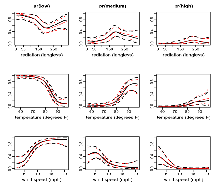
Figure 1: Ozone data. Posterior mean (solid lines) and $95\%$ interval estimates (dashed lines) for $\mathrm{Pr}(Y=l\mid x_{m},G)$ (thick black) compared to $\mathrm{Pr}(\gamma_{l-1}<Z\leq\gamma_{l}\mid x_{m},G)$ (red), for $l=1,2,3$ and $m=1,2,3$, giving the probability that ozone concentration is low, medium, and high over covariates radiation, temperature, and wind speed.

The model was applied to the ozone data, with response, $Y$, given by discretized ozone concentration, and covariates, $\boldsymbol{X}=$ $(X_{1},X_{2},X_{3})=$ (radiation, temperature, wind speed). To validate the inferences obtained from the DP mixture ordinal regression model, we compare results with the ones from a DP mixture of multivariate normals for the continuous vector $(Z,\boldsymbol{X})$, since the observations for ozone concentration, $Z$, are available on a continuous scale. The latter model corresponds to the density regression approach of Müller et al. (1996), extended with respect to the resulting inferences in Taddy and Kottas (2010). Here, it serves as a benchmark for our ordinal regression model, since it provides the best possible inference that can be obtained under the mixture modeling framework if no loss in information occurs by observing $Y$ rather than $Z$. We compare the univariate regression curves $\mathrm{Pr}(Y=l\mid x_{m},G)$ with $\mathrm{Pr}(\gamma_{l-1}<Z\leq\gamma_{l}\mid x_{m},G)$, for $l=1,2,3$, and $m=1,2,3$, the latter based on the mixture model for $(Z,\boldsymbol{X})$. Figure 1 compares posterior mean and $95\%$ interval estimates for the regression curves given each of the three covariates. The key result is that both sets of inferences uncover the same regression relationship trends. The only subtle differences are in the uncertainty bands which are overall slightly wider under the ordinal regression model. Also noteworthy is the fact that the ordinal regression mixture model estimates both relatively standard monotonic regression functions (e.g., for temperature) as well as non-linear effects for radiation.

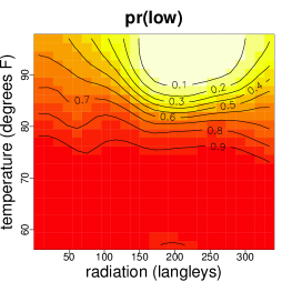
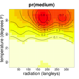
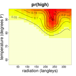
Figure 2: Ozone data. Posterior mean estimates for $\mathrm{Pr}(Y=l\mid x_{1},x_{2},G)$, for $l=1,2,3$, corresponding to, from left to right, low, medium, and high ozone concentration. The spectrum of colors from white to red indicates probabilities that range from 0 to 1.

The ability to capture such a wide range of trends for the regression relationships is a feature of the nonparametric mixture model. Another feature is its capacity to accommodate interaction effects among the covariates without the need to incorporate additional terms in the model. Such effects are suggested by the estimates for the response probability surfaces over pairs of covariates; for instance, Figure 2 displays these estimates as a function of radiation and temperature.

3.2 Credit ratings of U.S. companies

Here, we consider an example involving Standard and Poor’s (S&P) credit ratings for $921$ U.S. firms in 2005. The example is taken from Verbeek (2008), in which an ordered logit model was applied to the data, and was also used by Chib and Greenberg (2010) to illustrate an additive cubic spline regression model with a normal DP mixture error distribution. For each firm, a credit rating on a seven-point ordinal scale is available, along with five characteristics. Consistent with the analysis of Chib and Greenberg (2010), we combined the first two categories as well as the last two categories to produce an ordinal response with $5$ levels, where higher ratings indicate more creditworthiness. The covariates in this application are book leverage $X_{1}$ (ratio of debt to assets), earnings before interest and taxes divided by total assets $X_{2}$, standardized log-sales $X_{3}$ (proxy for firm size), retained earnings divided by total assets $X_{4}$ (proxy for historical profitability), and working capital divided by total assets $X_{5}$ (proxy for short-term liquidity).

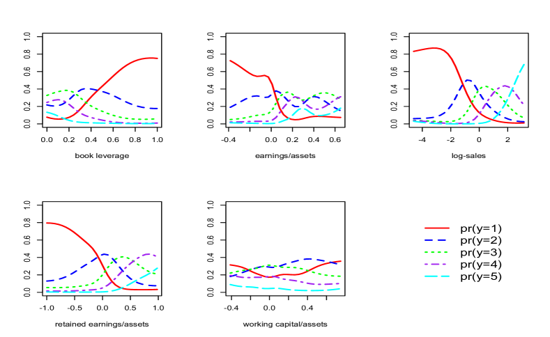
Figure 3: Credit rating data. Posterior mean estimates for $\mathrm{Pr}(Y=l\mid x_{m},G)$, for each covariate $m=1,\dots,5$. All five ordinal response curves are displayed in a single panel for each covariate.

The posterior mean estimates for the marginal probability curves, $\mathrm{Pr}(Y=l\mid x_{m},G)$, for $l=1,\dots,5$ and $m=1,\dots,5$, are shown in Figure 3. These estimates depict some differences from the corresponding ones reported in Chib and Greenberg (2010), which could be due to the additivity assumption of the covariate effects in the regression function under their model. Empirical regression functions – computed by calculating proportions of observations assigned to each class over a grid in each covariate – give convincing graphical evidence that the regression relationships estimated by our model fit the data quite well.

To discuss the estimated regression trends for one of the covariates, consider the standardized log-sales variable, which is a proxy for firm size. The probability of rating level $1$ is roughly constant for low log-sales values, and is then decreasing to $0$, indicating that small firms have a similar high probability of receiving the lowest rating, whereas the larger the firm, the closer to $0$ this probability becomes. The probability curves for levels $2$, $3$, and $4$ are all quadratic shaped, with peaks occurring at larger log-sales values for higher ratings. Finally, the probability of receiving the highest rating is very small for low to moderate log-sales values, and is increasing for larger values. In summary, log-sales are positively related to credit rating, as expected.

Figure 4: Credit rating data. Posterior mean (solid lines) and $95\%$ interval estimates (dashed lines) for covariate densities $f(x\mid Y=l,G)$ conditional on ordinal credit rating $l=1,...,5$. The top row corresponds to covariate book leverage, and the bottom row to standardized log-sales.

This is another example where it is arguably natural to model the joint distribution for the response and covariates (the specific firm characteristics). This allows our model to accommodate interactions between covariates, as we do not assume additivity or independence in the effects of the covariates on the latent response. In addition to the regression curve estimates, we may obtain inference for the covariate distribution, or for any covariate conditional on a specific ordinal rating. These inverse relationships (discussed in Section 2.4) could be practically relevant in this application. It may be of interest to investors and econometricians to know, for example, approximately how large is a company’s leverage, given that it has a rating of $2$? Is the distribution of leverage much different from that of a level $3$ company? Figure 4 plots the estimated densities for book leverage and standardized log-sales conditional on each of the five ordinal ratings. In general, the distribution of book leverage is centered on smaller values as rating increases, and the densities become more peaked supporting a smaller range of leverage values for higher ratings. The interval bands are slightly wider for the distribution associated with $Y=1$ than for $Y=2$, $3$, or $4$, and they are much wider for $Y=5$, which is consistent with the small number of firms with a rating of $5$. The distribution of log-sales has a mode which occurs at increasing values as rating increases, indicating that if one firm has a higher rating than another, it likely also has higher sales.

3.3 Standard and Poor’s grades of countries

As a second econometrics example, we consider a data set from Simonoff (2003), comprising S&P ratings of $n=31$ countries along with debt service ratio and income, the latter recorded on an ordinal scale with levels of low, medium, and high. Ratings range from 1 to 7, with 1 indicating the best rating of AAA, and 7 the worst of CCC. With two covariates and a very small sample size, this example provides an interesting testbed for our modeling approach.

Since income is available as a discrete variable, $W$, we model it through the (latent) continuous income variable, $Z_{2}$. Therefore, $X$ represents debt service ratio, and $\boldsymbol{Z}=$ $(Z_{1},Z_{2})$, where $W$ arises from $Z_{2}$ just as the ordinal rating response $Y$ arises through latent continuous response $Z_{1}$. This is another application where one may be interested in inverse relationships, such as the distribution of debt service ratio and/or income given a specific S&P rating.

The probability response curves as functions of debt service ratio (Figure 5) contain both monotonic trends (decreasing for response categories 1 and 2, and increasing for category 7), as well as non-linear ones, most notably for categories 4 and 5. The interval bands are wider than in earlier examples, given the smaller sample size. Although not shown here, regression curves can also be obtained over discrete income from $\mathrm{Pr}(Y=j\mid W=w,G)=$ $\mathrm{Pr}(Y=j,W=w\mid G)/\mathrm{Pr}(W=w\mid G)$, for $w=1,2,3$ (low, medium, and high income), where the numerator contains a double integral of a bivariate normal density function. The probability of receiving a top rating of 1, 2, or 3 is highest for high-income countries, the probability of receiving a moderate rating of 4 or 5 is highest for medium-income countries, and the probability of receiving a poor rating is highest for low-income countries. It is highly unlikely for a country to receive one of the top two ratings unless it is high-income, however there is non-negligible probability of a medium-income country receiving one of the two lowest ratings.

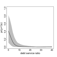
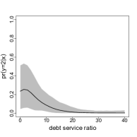
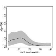
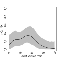
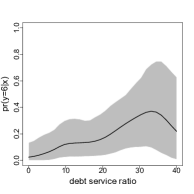
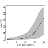
Figure 5: S&P ratings of countries data. Posterior mean (solid lines) and $95\%$ intervals (gray bands) for the probability response curve associated with each rating, ranging from AAA (level 1) to CCC (level 7), as a function of debt service ratio.

The latent continuous responses represent latent continuous credit rating in this application. The method for posterior simulation involves sampling $z_{i,1}$, for $i=1,\dots,31$, which represent the country-specific latent ratings. The two countries with AA (level 2) rating are Canada and Australia. Both of these countries have income classified as high, however Canada has no debt, whereas Australia has a debt service ratio which is around 10. This value is not particularly high, but since higher debt service ratio seems to be associated with poorer ratings, we would expect that Canada would be closer to receiving a better rating of AAA than Australia. Indeed, posterior densities of latent continuous ratings for Canada and Australia (Figure 6, left panel) indicate that Canada’s ordinal rating of AA is closer to a AAA rating than Australia’s.

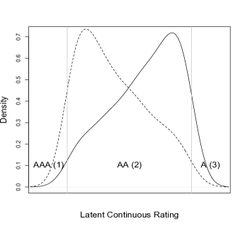
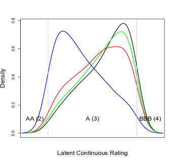
Figure 6: S&P ratings of countries data. Left panel: Posterior densities of latent continuous ratings for Australia (solid line) and Canada (dashed line), the two countries with AA rating. Right panel: Posterior densities of latent continuous ratings for the four countries with A rating: Chile (black), Czech Republic (red), Hungary (green), and Slovenia (blue). In both panels, the gray vertical lines indicate the borders for ordinal ratings.

Next, consider the four countries with A rating (level 3): Chile, Czech Republic, Hungary, and Slovenia. The first three of these countries are classified as medium income, whereas Slovenia is a high income country. The debt service ratios range from 8.9 (Czech Republic) to 15.8 (Chile). The estimated latent response densities are shown on the right panel of Figure 6. We note that Slovenia’s latent rating distribution is centered on values close to the cut-off point for a better rating of AA. The other three distributions are fairly similar. Chile appears closest to a BBB rating, which is consistent with its higher debt service ratio. An interesting observation from these results is that differences in income appear to have a larger effect on the latent rating distributions than differences in debt service ratio.

3.4 Analysis of multirater agreement data

A variety of methods exist for analyzing ordinal data collected from multiple raters when the goal is to measure agreement. Such methods range from the commonly used $\kappa$ statistic (Cohen, 1960) and its extensions (Fleiss, 1971), which are indices calculated from the observed and expected agreement of raters, to model-based approaches involving log-linear models (Tanner and Young, 1985). We do not attempt a comprehensive review here, rather our focus lies in the use of model-based methods for ordinal responses collected from multiple raters along with covariate information. The proposed multivariate ordinal regression model offers flexibility in this setting in terms of the modeling framework and resulting inferences. We focus on a scenario involving a set of expert graders who evaluate student essays, rating them on an ordinal scale. We contrast our approach to the parametric model of Johnson and Albert (1999), from where the specific data example is taken, and the semiparametric approach of Savitsky and Dalal (2014), both developing Bayesian inference built from modeling for latent responses.

Multirater agreement data arises when $k$ raters assign ordinal scores to $n$ individuals, such that $\boldsymbol{y}_{i}=$ $(y_{i1},\dots,y_{ik})$ collects all scores for the $i$th individual. The raters typically use the same classification levels, and therefore each $y_{ij}\in\{1,\dots,C\}$. This data structure could be summarized in a contingency table, however, we are concerned with problems in which relevant covariate information is available for each individual. We assume that each judge assigns an ordinal rating to individual $i$, which represents a discretized version of a continuous rating; that is, $y_{ij}$ is determined by $z_{ij}$, the continuous latent score assigned by judge $j$ on individual $i$.

This is in contrast to the formulation of Johnson and Albert (1999), where all judges are assumed to agree on the intrinsic worth of each item, such that $z_{ij}=w_{i}+\epsilon_{ij}$, where $w_{i}$ represents the true latent score, and $\epsilon_{ij}$ is the error observed by judge $j$. Then, $w_{i}$ is linearly related to the covariates, assumed normal with mean containing the term $\boldsymbol{x}_{i}^{T}\boldsymbol{\beta}$. The normal latent response distribution is not appropriate when grade distributions are skewed or favor low/high scores over moderate scores. Since the distribution of the $z_{ij}$ does not have a judge-specific mean, random cut-offs are necessary to allow the ratings of a particular subject to vary among judges.

Savitsky and Dalal (2014) note that the assumption of intrinsic agreement among raters may be inappropriate when raters have different beliefs or perspectives that may influence their scoring behavior. They assume a DP mixture model for the judge-specific latent random vectors built from a mixture kernel defined through independent normals. Dependence is therefore introduced over the latent scores of a single rater (albeit under a restrictive product-kernel for the mixture), but the data vectors arising from each rater are assumed independent. Under this model, it is therefore unclear how to extract inference for inter-rater agreement, which is a key inferential objective for applications of this type in the social sciences.

Similar to the approach in Savitsky and Dalal (2014), there is no notion in our model of an intrinsic true score for an individual. An overall score for an individual could be obtained by averaging in some fashion over the latent scores assigned by each rater. However, our main goal here is to obtain inference about relationships between the ordinal scores and the covariates, as well as for inter-rater agreement over both the covariate space and the scores. Our method offers a potentially useful perspective for modeling multirater agreement data, most notably with respect to the generality of the nonparametric mixture model which can accommodate complex dependence among raters and non-linear relationships with the random covariates.

We apply our method to a problem involving three expert graders who evaluate $n=198$ student essays, each assigned a rating on an ordinal scale of $1$ through $10$ (these represent raters 2, 3, and 4 from the data given in Chapter 5 of Johnson and Albert, 1999). Average word length and total number of essay words are used as the $p=2$ covariates, to study if they have an effect on grader ratings. The traditional measure of agreement between raters $l$ and $m$ in the social sciences, the polychoric correlation $\rho_{lm}=$ $\text{corr}(Z_{l},Z_{m})$, can be assessed through the covariance mixing parameters $(\boldsymbol{\Sigma}_{1},\dots,\boldsymbol{\Sigma}_{N})$. As discussed in Section 2.4, the posterior predictive distribution for $\rho_{lm}$ can be obtained by sampling at each MCMC iteration the corresponding $(\rho_{lm,1},\dots,\rho_{lm,N})$ with probabilities $(p_{1},\dots,p_{N})$. The polychoric correlation predictive distributions for all three pairs of raters favor more heavily positive correlations (raters 1 and 3 appear to agree most strongly), but place substantial probability on negative correlations. We can study where raters $l$ and $m$ tend to agree or disagree by grouping the latent continuous ratings according to the strength and direction of $\text{corr}(Z_{l},Z_{m})$. For instance, a plot of $\text{E}(z_{il}\mid\text{data})$ and $\text{E}(z_{im}\mid\text{data})$ arranged by $\text{E}(\text{corr}(z_{il},z_{im})\mid\text{data})$ reveals that raters 1 and 2 strongly agree on very low ratings, but disagree when rater 2 assigns low ratings and rater 1 high ratings. It is also the case for the other pairs of raters that they strongly agree mainly at low scores.

The model provides a variety of inferences in this multivariate ordinal regression example, which can be used to assess how ratings vary across covariates, as well as how raters behave in comparison to one another. Defining a high rating as 8 or higher, and a low rating as 3 or lower, Figure 7 plots estimates for the probability of high and low rating in terms of average word length and total number of words. There appears to be a strong trend in rating as a function of number of words for each rater, with rater 2 in particular assigning higher ratings for essays with more words. The regression curves for high ratings associated with rater 2 are somewhat separated from raters 1 and 3, suggesting that overall rater 2 assigns higher ratings.

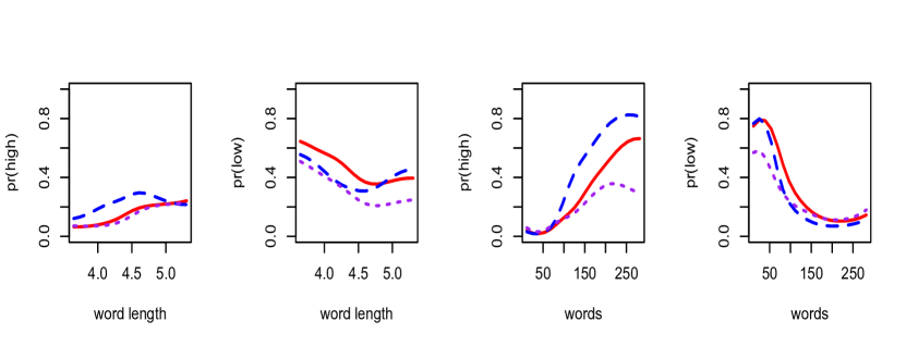
Figure 7: Multirater data. Posterior mean estimates for probability of high and low rating as a function of average word length (two left plots) and total number of words (two right plots), for raters 1 (solid red lines), 2 (dashed blue lines), and 3 (dotted purple lines).

To identify regions of the covariate space in which raters tend to agree or disagree, Figure 8 plots estimates for the probability of perfect agreement for the three pairs of raters as a function of total number of words. This inference suggests that raters 1 and 2 agree most strongly on grades for essays with few or many words. The trend in probability of agreement is weaker for the other two pairs of raters.

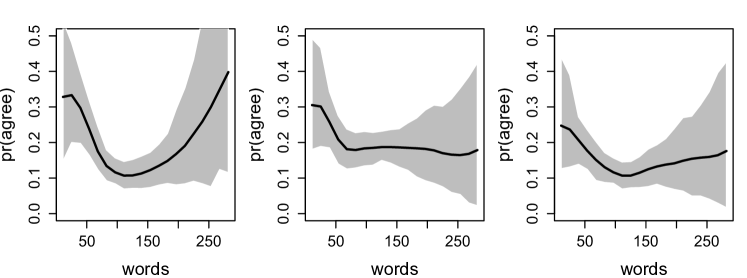
Figure 8: Multirater data. Posterior mean (solid lines) and $95\%$ interval estimates (gray bands) for probability of agreement as a function of total number of words. The left panel corresponds to raters 1 and 2, the middle panel to raters 1 and 3, and the right panel to raters 2 and 3.

Finally, to assess the strength of agreement between raters on high and low scores, we study the probability that one rater gives a high/low rating, conditional on the rating given by another rater. Table 1 includes posterior means for $\mathrm{Pr}(Y_{l}\mid Y_{m},G)$, for $l,m\in\{1,2,3\}$, with $Y_{l}$ and $Y_{m}$ taking values of $\{8,9,10\}$ (high) or $\{1,2,3\}$ (low). Each row represents the event being conditioned on, while each column represents the event a probability is being assigned to. For example, row 1, column 3 contains the posterior mean for $\mathrm{Pr}(Y_{2}\in\{8,9,10\}\mid Y_{1}\in\{8,9,10\},G)$. The cells corresponding to disagreement are highlighted with gray. The first two rows give probabilities conditional on rater 1 scores, and indicate that rater 2 has more disagreement with rater 1 than does rater 3. The last two rows suggest that rater 2 disagrees more with rater 3 than does rater 1. Finally, from the middle two rows, we note slightly more disagreement between raters 1 and 2 than between raters 3 and 2.

	$Y_{1}=\mathrm{H}$	$Y_{1}=\mathrm{L}$	$Y_{2}=\mathrm{H}$	$Y_{2}=\mathrm{L}$	$Y_{3}=\mathrm{H}$	$Y_{3}=\mathrm{L}$
$Y_{1}=\mathrm{H}$			$0.54$	$0.15$	$0.46$	$0.06$
$Y_{1}=\mathrm{L}$			$0.13$	$0.48$	$0.04$	$0.51$
$Y_{2}=\mathrm{H}$	$0.36$	$0.18$			$0.27$	$0.14$
$Y_{2}=\mathrm{L}$	$0.08$	$0.56$			$0.07$	$0.41$
$Y_{3}=\mathrm{H}$	$0.63$	$0.11$	$0.55$	$0.18$
$Y_{3}=\mathrm{L}$	$0.04$	$0.78$	$0.15$	$0.54$

Table 1: Multirater data. Posterior means for agreement and disagreement conditional probabilities for pairs of raters, with disagreement highlighted in gray (see Section 3.4 for details). H refers to high ratings of $\{8,9,10\}$, and L refers to low ratings of $\{1,2,3\}$.

4 Discussion

Seeking to expand Bayesian nonparametric methodology for ordinal regression, we have presented a fully nonparametric approach to modeling multivariate ordinal responses along with covariates. The inferential power of the framework lies in the flexible DP mixture model for the latent responses and covariates. The assumption of random covariates is appropriate for many problems, and modeling the covariates along with the latent responses accounts for dependence or interactions among the covariates. This also allows for inference on functionals of the covariate distribution. By establishing its KL support, we have shown that the prior probability model can accommodate general mixed ordinal-continuous distributions, without imputing cut-off points or restricting the covariance matrix of the normal kernel for the DP mixture model. From a practical point of view, this is a particularly appealing feature of the modeling approach relative to the multivariate probit model and related semiparametric extensions.

The multivariate normal mixture kernel can accommodate any type of continuous covariates (using transformation as needed). Discrete ordinal covariates can also be included by introducing latent continuous variables; this was implemented in the example of Section 3.3, in which the continuous covariate income was recorded on an ordinal scale. In order to handle discrete nominal covariates, the kernel can be modified adding appropriate components to the multivariate normal density, using either a marginal or conditional specification (e.g., Taddy and Kottas, 2010).

The version of the multivariate probit model discussed in the Introduction, and the setting we consider for our model, involves a common vector of covariates $\boldsymbol{X}=$ $(X_{1},...,X_{p})$ for each response vector $\boldsymbol{Y}$. That is, the covariates are not specific to particular response variables, but rather $(\boldsymbol{Y},\boldsymbol{X})$ arises as a multivariate vector. An alternative version of the probit model involves $p_{j}$ covariates $(X_{j,1},\dots,X_{j,p_{j}})$ specific to response variable $Y_{j}$. This regression setting was described for multivariate continuous responses by Tiao and Zellner (1964), and this is the version of the multivariate binary probit model considered in Chib and Greenberg (1998).

Scenarios which make use of response specific covariates fall broadly into two categories. The first consists of problems in which only a portion of the covariate vector is thought to affect a particular response, but there may be some overlap in the subset of covariates which generate the responses. Chib and Greenberg (1998) considered a voting behavior problem of this kind in which the first of two responses was assumed to be generated by a subset of the covariates associated with the second response. This data structure can also be accommodated by modeling all covariates $\boldsymbol{X}$ jointly with $\boldsymbol{Y}$, and conditioning on the relevant subset of $\boldsymbol{X}$ in the regression inferences.

The other type of data structure which is occasionally handled with a multivariate regression model with response specific covariates involves univariate ordinal responses that are related in a hierarchical/dynamic fashion. For instance, Chib and Greenberg (1998) illustrate their model with the commonly used Six Cities data, in which $\boldsymbol{Y}=(Y_{1},\dots,Y_{4})$ represents wheezing status at ages $7$ through $10$. Such settings are arguably more naturally approached through hierarchical/dynamic modeling. Indeed, a possible extension of the methodology developed here involves dynamic modeling for ordinal regression relationships, such that at any particular time point a unique regression relationship is estimated in a flexible fashion, while dependence is incorporated across time.

Appendix A: Proof of Lemma 1

Under the normal kernel, $\text{N}(\boldsymbol{z},\boldsymbol{x}\mid\boldsymbol{\mu},\boldsymbol{\Sigma})$, of the DP mixture model for the latent responses, $\boldsymbol{z}=$ $(z_{1},...,z_{k})$, and covariates, $\boldsymbol{x}$, the kernel of the implied mixture model for the ordinal responses, $\boldsymbol{y}=$ $(y_{1},...,y_{k})$, and covariates is given by $k(\boldsymbol{y},\boldsymbol{x}\mid\boldsymbol{\mu},\boldsymbol{\Sigma})=$ $\int_{\gamma_{k,y_{k}-1}}^{\gamma_{k,y_{k}}}\cdot\cdot\cdot\int_{\gamma_{1,y_{1}-1}}^{\gamma_{1,y_{1}}}\text{N}(\boldsymbol{z},\boldsymbol{x}\mid\boldsymbol{\mu},\boldsymbol{\Sigma})\text{d}z_{1}\dots\text{d}z_{k}$. We assume fixed cut-off points, and $y_{j}\in\{1,\dots,C_{j}\}$ with $C_{j}>2$, for $j=1,\dots,k$.

We establish likelihood identifiability for parameters $\boldsymbol{\mu}$ and $\boldsymbol{\Sigma}$ in $k(\boldsymbol{y},\boldsymbol{x}\mid\boldsymbol{\mu},\boldsymbol{\Sigma})$. That is, from

$$k(\boldsymbol{y},\boldsymbol{x}\mid\boldsymbol{\mu}_{1},\boldsymbol{\Sigma}_{1})=k(\boldsymbol{y},\boldsymbol{x}\mid\boldsymbol{\mu}_{2},\boldsymbol{\Sigma}_{2}),$$ (7)

for all $(\boldsymbol{y},\boldsymbol{x})$, with $y_{j}\in\{1,\dots,C_{j}\}$ and $\boldsymbol{x}\in\mathbb{R}^{p}$, we will obtain $\boldsymbol{\mu}_{1}=\boldsymbol{\mu}_{2}$ and $\boldsymbol{\Sigma}_{1}=\boldsymbol{\Sigma}_{2}$.

Marginalizing over $\boldsymbol{y}$ both sides of (7), we obtain $\text{N}(\boldsymbol{x}\mid\boldsymbol{\mu}_{1}^{x},\boldsymbol{\Sigma}_{1}^{xx})=$ $\text{N}(\boldsymbol{x}\mid\boldsymbol{\mu}_{2}^{x},\boldsymbol{\Sigma}_{2}^{xx})$, for all $\boldsymbol{x}\in\mathbb{R}^{p}$, and thus $\boldsymbol{\mu}_{1}^{x}=$ $\boldsymbol{\mu}_{2}^{x}\equiv$ $\boldsymbol{\mu}^{x}$, and $\boldsymbol{\Sigma}_{1}^{xx}=$ $\boldsymbol{\Sigma}_{2}^{xx}\equiv$ $\boldsymbol{\Sigma}^{xx}$. We also have from (7) that for each $j=1,\dots,k$, $k(y_{j}\mid\boldsymbol{x},\boldsymbol{\mu}_{1},\boldsymbol{\Sigma}_{1})=$ $k(y_{j}\mid\boldsymbol{x},\boldsymbol{\mu}_{2},\boldsymbol{\Sigma}_{2})$, for all $y_{j}\in\{1,\dots,C_{j}\}$ and $\boldsymbol{x}\in\mathbb{R}^{p}$. Hence, $\text{Pr}(Y_{j}\leq l\mid\boldsymbol{x},\boldsymbol{\mu}_{1},\boldsymbol{\Sigma}_{1})=$ $\text{Pr}(Y_{j}\leq l\mid\boldsymbol{x},\boldsymbol{\mu}_{2},\boldsymbol{\Sigma}_{2})$, for $l=1,\dots,C_{j}-1$, and for all $\boldsymbol{x}\in\mathbb{R}^{p}$. That is,

$$\Phi\left(\frac{\gamma_{j,l}-\mu_{1}^{z_{j}}-\boldsymbol{\Sigma}_{1}^{z_{j}x}(\boldsymbol{\Sigma}^{xx})^{-1}(\boldsymbol{x}-\boldsymbol{\mu}^{x})}{({\Sigma}_{1}^{z_{j}z_{j}}-\boldsymbol{\Sigma}_{1}^{z_{j}x}(\boldsymbol{\Sigma}^{xx})^{-1}\boldsymbol{\Sigma}_{1}^{xz_{j}})^{1/2}}\right)=\Phi\left(\frac{\gamma_{j,l}-\mu_{2}^{z_{j}}-\boldsymbol{\Sigma}_{2}^{z_{j}x}(\boldsymbol{\Sigma}^{xx})^{-1}(\boldsymbol{x}-\boldsymbol{\mu}^{x})}{({\Sigma}_{2}^{z_{j}z_{j}}-\boldsymbol{\Sigma}_{2}^{z_{j}x}(\boldsymbol{\Sigma}^{xx})^{-1}\boldsymbol{\Sigma}_{2}^{xz_{j}})^{1/2}}\right),$$ (8)

for all $\boldsymbol{x}\in\mathbb{R}^{p}$, and for $l=1,\dots,C_{j}-1$. Because $\Phi(\cdot)$ is an increasing function, its arguments in equation (8) must be equal. The resulting equation can be expressed in the form $\boldsymbol{a}^{T}\boldsymbol{x}+b=0$. For this equation to hold true for any $\boldsymbol{x}$, we must have $\boldsymbol{a}=\boldsymbol{0}$ and $b=0$, which yield

$$\frac{\boldsymbol{\Sigma}_{1}^{z_{j}x}}{({\Sigma}_{1}^{z_{j}z_{j}}-\boldsymbol{\Sigma}_{1}^{z_{j}x}(\boldsymbol{\Sigma}^{xx})^{-1}\boldsymbol{\Sigma}_{1}^{xz_{j}})^{1/2}}=\frac{\boldsymbol{\Sigma}_{2}^{z_{j}x}}{({\Sigma}_{2}^{z_{j}z_{j}}-\boldsymbol{\Sigma}_{2}^{z_{j}x}(\boldsymbol{\Sigma}^{xx})^{-1}\boldsymbol{\Sigma}_{2}^{xz_{j}})^{1/2}},$$ (9)

and

$$\frac{\gamma_{j,l}-\mu_{1}^{z_{j}}+\boldsymbol{\Sigma}_{1}^{z_{j}x}(\boldsymbol{\Sigma}^{xx})^{-1}\boldsymbol{\mu}^{x}}{({\Sigma}_{1}^{z_{j}z_{j}}-\boldsymbol{\Sigma}_{1}^{z_{j}x}(\boldsymbol{\Sigma}^{xx})^{-1}\boldsymbol{\Sigma}_{1}^{xz_{j}})^{1/2}}=\frac{\gamma_{j,l}-\mu_{2}^{z_{j}}+\boldsymbol{\Sigma}_{2}^{z_{j}x}(\boldsymbol{\Sigma}^{xx})^{-1}\boldsymbol{\mu}^{x}}{({\Sigma}_{2}^{z_{j}z_{j}}-\boldsymbol{\Sigma}_{2}^{z_{j}x}(\boldsymbol{\Sigma}^{xx})^{-1}\boldsymbol{\Sigma}_{2}^{xz_{j}})^{1/2}},$$ (10)

for $l=1,\dots,C_{j}-1$. Using (9), (10) can be expressed as $(\gamma_{j,l}-\mu_{1}^{z_{j}})\boldsymbol{\Sigma}_{2}^{z_{j}x}=$ $(\gamma_{j,l}-\mu_{2}^{z_{j}})\boldsymbol{\Sigma}_{1}^{z_{j}x}$, for each $j=1,...,k$. Working with $2$ of these $C_{j}-1$ equations, the system can be shown to have solution $\boldsymbol{\Sigma}_{1}^{z_{j}x}=$ $\boldsymbol{\Sigma}_{2}^{z_{j}x}\equiv$ $\boldsymbol{\Sigma}^{z_{j}x}$. Then, from (10) and (9), we obtain $\mu_{1}^{z_{j}}=$ $\mu_{2}^{z_{j}}\equiv$ $\mu^{z_{j}}$ and ${\Sigma}_{1}^{z_{j}z_{j}}=$ ${\Sigma}_{2}^{z_{j}z_{j}}\equiv$ ${\Sigma}^{z_{j}z_{j}}$, respectively.

Notice that we required $2$ of the $C_{j}-1$ equations of the form in (10) to arrive at this solution. If $C_{j}=2$ for some $j$, we are unable to identify the full covariance matrix $\boldsymbol{\Sigma}$. In this case, if we fix ${\Sigma}^{z_{j}z_{j}}$, we can identify $\mu^{z_{j}}$ and $\boldsymbol{\Sigma}^{z_{j}x}$, as in DeYoreo and Kottas (2015). Although we do not require free cut-offs here due to the flexibility provided by the mixture, if $C_{j}>3$, the cut-off points $\gamma_{j,3},\dots,\gamma_{j,C_{j}-1}$ are also identifiable.

Finally, we must establish identifiability for $\Sigma^{z_{j}z_{j^{\prime}}}$, where $j\neq j^{\prime}$. Note that (7) implies $k(y_{j},y_{j^{\prime}}\mid\boldsymbol{\mu}_{1},\boldsymbol{\Sigma}_{1})=$ $k(y_{j},y_{j^{\prime}}\mid\boldsymbol{\mu}_{2},\boldsymbol{\Sigma}_{2})$, for any $j,{j^{\prime}}\in\{1,\dots,k\}$, with $j\neq j^{\prime}$. Hence, for any $y_{j}\in\{1,\dots,C_{j}\}$ and $y_{j^{\prime}}\in\{1,\dots,C_{j^{\prime}}\}$, $\int_{\gamma_{j^{\prime},y_{j^{\prime}}-1}}^{\gamma_{j^{\prime},y_{j^{\prime}}}}\int_{\gamma_{{j},y_{j}-1}}^{\gamma_{{j},y_{{j}}}}\text{N}((z_{j},z_{j^{\prime}})^{T}\mid(\mu^{z_{j}},\mu^{z_{j^{\prime}}})^{T},\boldsymbol{V}_{1})\,\text{d}z_{j}\text{d}z_{j^{\prime}}$ $=\int_{\gamma_{j^{\prime},y_{j^{\prime}}-1}}^{\gamma_{j^{\prime},y_{j^{\prime}}}}\int_{\gamma_{{j},y_{j}-1}}^{\gamma_{{j},y_{{j}}}}\text{N}((z_{j},z_{j^{\prime}})^{T}\mid(\mu^{z_{j}},\mu^{z_{j^{\prime}}})^{T},\boldsymbol{V}_{2})\,\text{d}z_{j}\text{d}z_{j^{\prime}}$. Here, matrices $\boldsymbol{V}_{1}$ and $\boldsymbol{V}_{2}$ have the same diagonal elements (given by ${\Sigma}^{z_{j}z_{j}}$ and ${\Sigma}^{z_{j^{\prime}}z_{j^{\prime}}}$) and off-diagonal element given by $\Sigma^{z_{j}z_{j^{\prime}}}_{1}$ and $\Sigma^{z_{j}z_{j^{\prime}}}_{2}$, respectively.

We will therefore obtain $\Sigma^{z_{j}z_{j^{\prime}}}_{1}=$ $\Sigma^{z_{j}z_{j^{\prime}}}_{2}$, for $j\neq j^{\prime}$, if the bivariate normal distribution function is increasing in the correlation parameter $\rho$ (assuming, without loss of generality, zero means and unit variances). To this end, note that $\frac{\partial}{\partial\rho}\text{N}((x,y)^{T}\mid\boldsymbol{0},\boldsymbol{R})=$ $\frac{\partial^{2}}{\partial x\partial y}\text{N}((x,y)^{T}\mid\boldsymbol{0},\boldsymbol{R})$, where $\boldsymbol{R}$ has unit diagonal elements, and off-diagonal element $\rho$ (e.g., Plackett, 1954). Therefore, $\frac{\partial}{\partial\rho}\int_{-\infty}^{a}\int_{-\infty}^{b}\text{N}((x,y)^{T}\mid\boldsymbol{0},\boldsymbol{R})\,\text{d}x\text{d}y=$ $\text{N}((a,b)^{T}\mid\boldsymbol{0},\boldsymbol{R})>0$, and thus the result is obtained.

Appendix B: Kullback-Leibler support for the model

We first prove Lemma 2 assuming (as in the statement of the lemma) that the true ordinal-continuous distribution $p_{0}(\boldsymbol{x},\boldsymbol{y})\in\mathcal{D^{*}}$ satisfies appropriate regularity conditions which imply that the corresponding density $f_{0}(\boldsymbol{x},\boldsymbol{z})\in\mathcal{D}$ is in the KL support of the prior. This result is general and it applies to any prior model for the latent continuous distribution which provides full KL support to $f_{0}$. Next, we provide a specific example for an $f_{0}$ that enables the connection with $p_{0}$ given in (6). And, using Theorem 2 of Wu and Ghosal (2008), we derive conditions for $p_{0}$ under which the corresponding $f_{0}$ is in the KL support of the DP location normal mixture prior model, thus validating Lemma 2 for our model.

B1. Proof of Lemma 2

Let $\mathrm{KL}(f_{0},f)=$ $\int f_{0}(w)\log(f_{0}(w)/f(w))\text{d}w$ be the KL divergence between densities $f_{0}$ and $f$. Based on the chain rule for relative entropy,

$$\mathrm{KL}(f_{0}(\boldsymbol{x},\boldsymbol{z}),f(\boldsymbol{x},\boldsymbol{z}))=\mathrm{KL}(f_{0}(\boldsymbol{x}),f(\boldsymbol{x}))+\mathrm{KL}(f_{0}(\boldsymbol{z}\mid\boldsymbol{x}),f(\boldsymbol{z}\mid\boldsymbol{x}))$$

where the KL divergence between conditional densities is defined as $\mathrm{KL}(f_{0}(\boldsymbol{z}\mid\boldsymbol{x}),f(\boldsymbol{z}\mid\boldsymbol{x}))=$ $\int f_{0}(\boldsymbol{x})\{\int f_{0}(\boldsymbol{z}\mid\boldsymbol{x})\log(f_{0}(\boldsymbol{z}\mid\boldsymbol{x})/f(\boldsymbol{z}\mid\boldsymbol{x}))\text{d}\boldsymbol{z}\}\text{d}\boldsymbol{x}$. Hence, $\mathrm{KL}(f_{0}(\boldsymbol{x}),f(\boldsymbol{x}))\leq$ $\mathrm{KL}(f_{0}(\boldsymbol{x},\boldsymbol{z}),f(\boldsymbol{x},\boldsymbol{z}))$, and thus, for any $\epsilon>0$, $K_{\epsilon}(f_{0}(\boldsymbol{x},\boldsymbol{z}))\subseteq$ $K_{\epsilon}(f_{0}(\boldsymbol{x}))=$ $\{f(\boldsymbol{x},\boldsymbol{z}):\mathrm{KL}(f_{0}(\boldsymbol{x}),f(\boldsymbol{x}))<\epsilon\}$. Using the KL property of the prior model for $f(\boldsymbol{x},\boldsymbol{z})$, $\mathcal{P}(K_{\epsilon}(f_{0}(\boldsymbol{x})))\geq\mathcal{P}(K_{\epsilon}(f_{0}(\boldsymbol{x},\boldsymbol{z})))>0$, such that the prior assigns positive probability to all KL neighborhoods of the true covariate density $f_{0}(\boldsymbol{x})$.

The proof relies on the following inequality for two densities $g_{1}(\boldsymbol{t})$ and $g_{2}(\boldsymbol{t})$, where $\boldsymbol{t}\in\mathbb{R}^{s}$, and for general subsets $A_{1},...,A_{s}$ of $\mathbb{R}$,

$$\int_{A_{s}}\cdot\cdot\cdot\int_{A_{1}}g_{1}(\boldsymbol{t})\log\left(\frac{g_{1}(\boldsymbol{t})}{g_{2}(\boldsymbol{t})}\right)\text{d}\boldsymbol{t}\geq\int_{A_{s}}\cdot\cdot\cdot\int_{A_{1}}g_{1}(\boldsymbol{t})\text{d}\boldsymbol{t}\times\log\left(\frac{\int_{A_{s}}\cdot\cdot\cdot\int_{A_{1}}g_{1}(\boldsymbol{t})\text{d}\boldsymbol{t}}{\int_{A_{s}}\cdot\cdot\cdot\int_{A_{1}}g_{2}(\boldsymbol{t})\text{d}\boldsymbol{t}}\right).$$ (11)

To prove the inequality, let $B_{r}=$ $\int_{A_{s}}\cdot\cdot\cdot\int_{A_{1}}g_{r}(\boldsymbol{t})\text{d}\boldsymbol{t}$, for $r=1,2$, such that $h_{r}(\boldsymbol{t})=$ $g_{r}(\boldsymbol{t})/B_{r}$, $r=1,2$, are densities on $A_{1}\times...\times A_{s}$. Then, the left-hand-side of (11) can be written as $B_{1}\int_{A_{s}}\cdot\cdot\cdot\int_{A_{1}}h_{1}(\boldsymbol{t})\log\left(\frac{B_{1}h_{1}(\boldsymbol{t})}{B_{2}h_{2}(\boldsymbol{t})}\right)\text{d}\boldsymbol{t}=$ $B_{1}\log(\frac{B_{1}}{B_{2}})$ + $B_{1}\int_{A_{s}}\cdot\cdot\cdot\int_{A_{1}}h_{1}(\boldsymbol{t})\log\left(\frac{h_{1}(\boldsymbol{t})}{h_{2}(\boldsymbol{t})}\right)\text{d}\boldsymbol{t}\geq$ $B_{1}\log(\frac{B_{1}}{B_{2}})$, since $\int_{A_{s}}\cdot\cdot\cdot\int_{A_{1}}h_{1}(\boldsymbol{t})\log\left(h_{1}(\boldsymbol{t})/h_{2}(\boldsymbol{t})\right)\text{d}\boldsymbol{t}$ is the KL divergence for densities $h_{1}$ and $h_{2}$.

Now, consider density $f(\boldsymbol{x},\boldsymbol{z})\in K_{\epsilon/2}(f_{0}(\boldsymbol{x},\boldsymbol{z}))$. By the chain rule, $\mathrm{KL}(f_{0}(\boldsymbol{x}),f(\boldsymbol{x}))<\epsilon/2$, and $\mathrm{KL}(f_{0}(\boldsymbol{z}\mid\boldsymbol{x}),f(\boldsymbol{z}\mid\boldsymbol{x}))<\epsilon/2$. We apply (11) with $s=k$, $g_{1}(\boldsymbol{t})=$ $f_{0}(\boldsymbol{z}\mid\boldsymbol{x})$, $g_{2}(\boldsymbol{t})=$ $f(\boldsymbol{z}\mid\boldsymbol{x})$, and $A_{j}=$ $(\gamma_{j,y_{j}-1},\gamma_{j,y_{j}})$, for $j=1,\dots,k$. This yields

$$\int_{\gamma_{k,y_{k}-1}}^{\gamma_{k,y_{k}}}\cdot\cdot\cdot\int_{\gamma_{1,y_{1}-1}}^{\gamma_{1,y_{1}}}f_{0}(\boldsymbol{z}\mid\boldsymbol{x})\log\left(\frac{f_{0}(\boldsymbol{z}\mid\boldsymbol{x})}{f(\boldsymbol{z}\mid\boldsymbol{x})}\right)\text{d}\boldsymbol{z}\geq p_{0}(\boldsymbol{y}\mid\boldsymbol{x})\log\left(\frac{p_{0}(\boldsymbol{y}\mid\boldsymbol{x})}{p^{*}(\boldsymbol{y}\mid\boldsymbol{x})}\right)$$ (12)

for any configuration of values $\boldsymbol{y}=$ $(y_{1},...,y_{k})$ for the ordinal responses. Here, $p^{*}(\boldsymbol{y}\mid\boldsymbol{x})=$ $\int_{\gamma_{k,y_{k}-1}}^{\gamma_{k,y_{k}}}\cdot\cdot\cdot\int_{\gamma_{1,y_{1}-1}}^{\gamma_{1,y_{1}}}f(\boldsymbol{z}\mid\boldsymbol{x})\text{d}\boldsymbol{z}$, such that $p^{*}(\boldsymbol{x},\boldsymbol{y})=$ $f(\boldsymbol{x})p^{*}(\boldsymbol{y}\mid\boldsymbol{x})$. Next, we sum both sides of (12) over $\boldsymbol{y}$, then multiply both sides by $f_{0}(\boldsymbol{x})$, and finally integrate both sides over $\boldsymbol{x}$, to obtain

$$\int_{\mathbb{R}^{p}}f_{0}(\boldsymbol{x})\int_{\mathbb{R}^{k}}f_{0}(\boldsymbol{z}\mid\boldsymbol{x})\log\left(\frac{f_{0}(\boldsymbol{z}\mid\boldsymbol{x})}{f(\boldsymbol{z}\mid\boldsymbol{x})}\right)\text{d}\boldsymbol{z}\text{d}\boldsymbol{x}\geq\int_{\mathbb{R}^{p}}f_{0}(\boldsymbol{x})\sum_{y_{k}=1}^{C_{k}}\cdot\cdot\cdot\sum_{y_{1}=1}^{C_{1}}p_{0}(\boldsymbol{y}\mid\boldsymbol{x})\log\left(\frac{p_{0}(\boldsymbol{y}\mid\boldsymbol{x})}{p^{*}(\boldsymbol{y}\mid\boldsymbol{x})}\right)\text{d}\boldsymbol{x}$$

that is, $\mathrm{KL}(f_{0}(\boldsymbol{z}\mid\boldsymbol{x}),f(\boldsymbol{z}\mid\boldsymbol{x}))\geq$ $\mathrm{KL}(p_{0}(\boldsymbol{y}\mid\boldsymbol{x}),p^{*}(\boldsymbol{y}\mid\boldsymbol{x}))$. Since $\mathrm{KL}(f_{0}(\boldsymbol{z}\mid\boldsymbol{x}),f(\boldsymbol{z}\mid\boldsymbol{x}))<\epsilon/2$, we have $\mathrm{KL}(p_{0}(\boldsymbol{y}\mid\boldsymbol{x}),p^{*}(\boldsymbol{y}\mid\boldsymbol{x}))<\epsilon/2$, which in conjunction with $\mathrm{KL}(f_{0}(\boldsymbol{x}),f(\boldsymbol{x}))<\epsilon/2$, further implies $\mathrm{KL}(p_{0}(\boldsymbol{x},\boldsymbol{y}),p^{*}(\boldsymbol{x},\boldsymbol{y}))<\epsilon$, by the chain rule. We have thus obtained

$$K_{\epsilon/2}(f_{0}(\boldsymbol{x},\boldsymbol{z}))\subseteq K_{\epsilon/2}(p_{0}(\boldsymbol{y}\mid\boldsymbol{x}))\,\,\,\,\,\,\,\text{and}\,\,\,\,\,\,\,K_{\epsilon/2}(f_{0}(\boldsymbol{x},\boldsymbol{z}))\subseteq K_{\epsilon}(p_{0}(\boldsymbol{x},\boldsymbol{y}))$$

where $K_{\epsilon}(p_{0}(\boldsymbol{x},\boldsymbol{y}))=$ $\{f(\boldsymbol{x},\boldsymbol{z}):\mathrm{KL}(p_{0}(\boldsymbol{x},\boldsymbol{y}),p^{*}(\boldsymbol{x},\boldsymbol{y}))<\epsilon\}$, from which the result emerges using the KL property of the prior model for $f(\boldsymbol{x},\boldsymbol{z})$.

B2. Density $f_{0}$ and conditions for the true $p_{0}$

We first show that there exists at least one $f_{0}(\boldsymbol{x},\boldsymbol{z})\in\mathcal{D}$ for any $p_{0}(\boldsymbol{x},\boldsymbol{y})\in\mathcal{D^{*}}$, as defined in (6). Consider $y_{j}\in\{1,\dots,C_{j}\}$, for $j=1,...,k$, and define

$$f_{0}(\boldsymbol{x},\boldsymbol{z})=\sum_{y_{1}}\cdot\cdot\cdot\sum_{y_{k}}\frac{p_{0}(\boldsymbol{x},y_{1},\dots,y_{k})\prod_{j=1}^{k}1_{(\gamma^{*}_{j,y_{j}-1},\gamma^{*}_{j,y_{j}}]}(z_{j})}{\prod_{j=1}^{k}(\gamma^{*}_{j,y_{j}}-\gamma^{*}_{j,y_{j}-1})}$$ (13)

where $\gamma^{*}_{j,l}=\gamma_{j,l}$ if $l\in\{1,\dots,C_{j}-1\}$, $\gamma^{*}_{j,0}=b_{j}$, and $\gamma^{*}_{j,C_{j}}=d_{j}$, with $-\infty<b_{j}<\gamma_{j,1}$ and $\gamma_{j,C_{j}-1}<d_{j}<\infty$, for $j=1,\dots,k$. Then, $f_{0}(\boldsymbol{x},\boldsymbol{z})$ satisfies the relationship in (6).

The final item needed to show that Lemma 2 is applicable to our model is to develop conditions for the true $p_{0}$ under which the corresponding $f_{0}$ in (13) satisfies (5). To this end, we use Theorem 2 of Wu and Ghosal (2008), which provides nine conditions (B1 to B9) on the true density $f_{0}$ and on the kernel of a nonparametric mixture model such that the KL property is satisfied. Conditions B1, B2, B3 and B9 involve the mixture kernel, and as discussed in Wu and Ghosal (2008), are satisfied by the product normal kernel. Condition B8 involves the prior for the mixing distribution and is valid for the DP prior.

Conditions A, B, C and D stated below for the true $p_{0}$ are sufficient for the remaining conditions in Theorem 2 of Wu and Ghosal (2008) to hold. For simpler notation, we consider the special case of the model with a single ordinal response and a single covariate, such that $p_{0}(x,y)$ is a distribution on $\mathbb{R}\times\{1,...,C\}$, with $C\geq 2$. The conditions can be extended to the general setting with multiple ordinal responses and covariates.

A. There exists $0<M<\infty$ such that $0<p_{0}(x,y)\leq M$, for all $(x,y)\in\mathbb{R}\times\{1,...,C\}$.
B. $|\int p_{0}(x,y)\log(p_{0}(x,y)/W)\,\text{d}x|<\infty$, for all $y\in\{1,...,C\}$, and for any $W>0$.
C. There exists $\delta>0$ such that $\int p_{0}(x,y)\log(p_{0}(x,y)/\varphi_{\delta}(x,y))\,\text{d}x<\infty$, for all $y\in\{1,...,C\}$, where $\varphi_{\delta}(x,y)=$ $\inf_{|x^{\prime}-x|<\delta}p_{0}(x^{\prime},y)$.
D. There exist $\eta>0$ and $d>0$ such that $\int p_{0}(x,y)(x^{2}+d^{2})^{\eta}\,\text{d}x<\infty$ and $\int p_{0}(x,y)x^{2}(x^{2}+d^{2})^{\eta}\,\text{d}x<\infty$, for all $y\in\{1,...,C\}$. In addition, $\int p_{0}(x,y)\{(x-a)^{2}/(2v^{2})\}\,\text{d}x<\infty$, for all $y\in\{1,...,C\}$, and for any $a\in\mathbb{R}$ and $v>0$.

It is straightforward to verify that B4, B5, B6 and B7 in Theorem 2 of Wu and Ghosal (2008) are satisfied by $f_{0}$ in (13) under conditions A, B, C and D, respectively. The only additional assumption needed is that the cut-off points take positive values, which is without loss of generality under our model that uses fixed cut-offs.

Supplementary Materials

All supplemental files listed below are contained in a single .zip file (supplementary-files.zip) and can be obtained via a single download.

Ozone data:

ozone data file. (ozone.csv)

Credit rating data:

credit rating data. (credit.dat)

Countries data:

S&P ratings of countries. (countries.txt)

Multirater data:

data used in the ratings of student essays example. (essay.csv)

Code for ozone data:

Code for implementing ordinal regression model on ozone data. (ozone-code-paper, R file)

Code for credit rating data:

Code for implementing ordinal regression model on credit rating data. (credit-code-paper, R file)

Code for multirater data:

Code for implementing ordinal regression model on multirater data. (multirater-code-paper, R file)

MCMC supplement:

Additional material related to MCMC and computation. (supplementary-mcmc.pdf)

References

- Albert and Chib (1993) Albert, J. and Chib, S. (1993), “Bayesian analysis of binary and polychotomous response data.” Journal of the American Statistical Association, 88, 669–679.
- Bao and Hanson (2015) Bao, J. and Hanson, T. (2015), “Bayesian nonparametric multivariate ordinal regression,” Canadian Journal of Statistics, 43, 337–357.
- Basu and Mukhopadhyay (2000) Basu, S. and Mukhopadhyay, S. (2000), “Bayesian analysis of binary regression using symmetric and asymmetric links,” The Indian Journal of Statistics Series B, 62, 372–387.
- Boes and Winkelmann (2006) Boes, S. and Winkelmann, R. (2006), “Ordered response models,” Advances in Statistical Analysis, 90, 165–179.
- Canale and Dunson (2011) Canale, A. and Dunson, D. B. (2011), “Bayesian kernel mixtures for counts,” Journal of the American Statistical Association, 106, 1528–1539.
- Canale and Dunson (2015) — (2015), “Bayesian multivariate mixed-scale density estimation,” Statistics and Its Interface, 8, 195–201.
- Chen and Dey (2000) Chen, M. and Dey, D. (2000), “Bayesian analysis for correlated ordinal data models,” in Generalized Linear Models: A Bayesian Perspective, eds. Dey, D., Ghosh, S., and Mallick, B., New York: Marcel Dekker, pp. 135–162.
- Chib and Greenberg (1998) Chib, S. and Greenberg, E. (1998), “Analysis of multivariate probit models,” Biometrika, 85, 347–361.
- Chib and Greenberg (2010) — (2010), “Additive cubic spline regression with Dirichlet process mixture errors,” Journal of Econometrics, 156, 322–336.
- Choudhuri et al. (2007) Choudhuri, N., Ghosal, S., and Roy, A. (2007), “Nonparametric binary regression using a Gaussian process prior,” Statistical Methodology, 4, 227–243.
- Cohen (1960) Cohen, J. (1960), “A coefficient of agreement for nominal scales,” Educational and Psychological Measurement, 20, 37–46.
- Daniels and Pourahmadi (2002) Daniels, M. and Pourahmadi, M. (2002), “Bayesian analysis of covariance matrices and dynamic models for longitudinal data,” Biometrika, 89, 553–566.
- DeYoreo and Kottas (2015) DeYoreo, M. and Kottas, A. (2015), “A fully nonparametric modeling approach to binary regression,” Bayesian Analysis, 10, 821–847.
- Di Lucca et al. (2013) Di Lucca, M., Guglielmi, A., Müller, P., and Quintana, F. (2013), “A Simple Class of Bayesian Autoregression Models,” Bayesian Analysis, 8, 63–88.
- Dunson and Bhattacharya (2010) Dunson, D. and Bhattacharya, A. (2010), “Nonparametric Bayes regression and classification through mixtures of product kernels,” Bayesian Statistics, 9, 145–164.
- Escobar and West (1995) Escobar, M. and West, M. (1995), “Bayesian density estimation and inference using mixtures,” Journal of the American Statistical Association, 90, 577–568.
- Ferguson (1973) Ferguson, T. (1973), “A Bayesian analysis of some nonparametric problems,” The Annals of Statistics, 1, 209–230.
- Fleiss (1971) Fleiss, J. (1971), “Measuring nominal scale agreement among many raters,” Psychological Bulletin, 76, 378–382.
- Ghosh and Ramamoorthi (2003) Ghosh, J. and Ramamoorthi, R. (2003), Bayesian Nonparametrics, New York: Springer.
- Gill and Casella (2009) Gill, J. and Casella, G. (2009), “Nonparametric priors for ordinal Bayesian social science models: Specification and estimation,” Journal of the American Statistical Association, 104, 453–464.
- Hannah et al. (2011) Hannah, L., Blei, D., and Powell, W. (2011), “Dirichlet process mixtures of generalized linear models,” Journal of Machine Learning Research, 1, 1–33.
- Hobert and Casella (1996) Hobert, J. and Casella, G. (1996), “The effect of improper priors on Gibbs sampling in hierarchical linear mixed models,” Journal of the American Statistical Association, 61, 1461–1473.
- Imai and van Dyk (2005) Imai, K. and van Dyk, D. (2005), “A Bayesian analysis of the multivariate probit model using marginal data augmentation,” Journal of Econometrics, 124, 311–334.
- Ishwaran and James (2001) Ishwaran, H. and James, L. (2001), “Gibbs sampling methods for stick-breaking priors,” Journal of the American Statistical Association, 96, 161–173.
- Ishwaran and Zarepour (2000) Ishwaran, H. and Zarepour, M. (2000), “Markov chain Monte Carlo in approximate Dirichlet and Beta two-parameter process hierarchical models,” Biometrika, 87, 371–390.
- Johnson and Albert (1999) Johnson, V. and Albert, J. (1999), Ordinal Data Modeling, New York: Springer.
- Kalli et al. (2011) Kalli, M., Griffin, J., and Walker, S. (2011), “Slice Sampling Mixture Models,” Statistics and Computing, 21, 93–105.
- Koop (2003) Koop, G. (2003), Bayesian Econometrics, Chichester: John Wiley and Sons.
- Kottas et al. (2005) Kottas, A., Müller, P., and Quintana, F. (2005), “Nonparametric Bayesian modelling for multivariate ordinal data,” Journal of Computational and Graphical Statistics, 14, 610–625.
- Lawrence et al. (2008) Lawrence, E., Bingham, D., Liu, C., and Nair, V. (2008), “Bayesian inference for multivariate ordinal data using parameter expansion,” Technometrics, 50, 182–191.
- Liu (2001) Liu, C. (2001), “Bayesian analysis of multivariate probit models – discussion on the art of data augmentation by Van Dyk and Meng,” Journal of Computational and Graphical Statistics, 10, 75–81.
- Liu and Wu (1999) Liu, J. and Wu, Y. (1999), “Parameter expansion for data augmentation,” Journal of the American Statistical Assocation, 94, 1264–1274.
- McCulloch et al. (2000) McCulloch, P., Polson, N., and Rossi, P. (2000), “A Bayesian analysis of the multinomial probit model with fully identified parameters,” Journal of Econometrics, 99, 173–193.
- Mukhopadyay and Gelfand (1997) Mukhopadyay, S. and Gelfand, A. (1997), “Dirichlet process mixed generalized linear models,” Journal of the American Statistical Association, 92, 633–639.
- Müller et al. (1996) Müller, P., Erkanli, A., and West, M. (1996), “Bayesian curve fitting using multivariate normal mixtures,” Biometrika, 83, 67–79.
- Müller and Quintana (2010) Müller, P. and Quintana, F. (2010), “Random partition models with regression on covariates,” Journal of Statistical Planning and Inference, 140, 2801–2808.
- Neal (2000) Neal, R. (2000), “Markov Chain Sampling Methods for Dirichlet Process Mixture Models,” Journal of Computational and Graphical Statistics, 9, 249–265.
- Newton et al. (1996) Newton, M., Czado, C., and Chappell, R. (1996), “Bayesian inference for semiparametric binary regression,” Journal of the American Statistical Association, 91, 142–153.
- Norets and Pelenis (2012) Norets, A. and Pelenis, J. (2012), “Bayesian modeling of joint and conditional distributions,” Journal of Econometrics, 168, 332–346.
- Olsson (1979) Olsson, U. (1979), “Maximum likelihood estimation of the polychoric correlation coefficient,” Psychometrika, 44, 443–460.
- Papageorgiou et al. (2015) Papageorgiou, G., Richardson, S., and Best, N. (2015), “Bayesian nonparametric models for spatially indexed data of mixed type,” Journal of the Royal Statistical Society, Series B, 77, 973–999.
- Park and Dunson (2010) Park, J. H. and Dunson, D. B. (2010), “Bayesian generalized product partition model,” Statistica Sinica, 20, 1203–1226.
- Plackett (1954) Plackett, R. L. (1954), “A reduction formula for normal multivariate integrals,” Biometrika, 41, 351–360.