Composite fermion-boson mapping for fermionic lattice models

J. Zhao1, C. A. Jimรฉnez-Hoyos1, G. E. Scuseria1,2, D. Huerga3, J. Dukelsky3, S. M. A. Rombouts4, and G. Ortiz5 1 Department of Chemistry, Rice University, Houston, Texas 77005, USA 2 Department of Physics and Astronomy, Rice University, Houston, Texas 77005, USA 3 Instituto de Estructura de la Materia, CSIC, Serrano 123, E-28006 Madrid, Spain 4 Departamento de Fรญsica Aplicada, Universidad de Huelva, E-21071 Huelva, Spain 5 Department of Physics, Indiana University, Bloomington IN 47405, USA
Abstract

We present a mapping of elementary fermion operators onto a quadratic form of composite fermionic and bosonic cluster operators. The mapping is an exact isomorphism as long as the physical constraint of one composite particle per cluster is satisfied. This condition is treated on average in a composite particle mean-field approach, which consists of an ansatz that decouples the composite fermionic and bosonic sectors. The theory is tested on the one- and two-dimensional Hubbard models. Using a Bogoliubov determinant for the composite fermions and either a coherent or Bogoliubov state for the bosons, we obtain a simple and accurate procedure for treating the Mott insulating phase of the Hubbard model with mean-field computational cost.

1 Introduction

The Hubbard model is a prototypical example of a strongly correlated system characterized by the competition between the strong particle interaction ($U$) and the kinetic energy ($t$). It is exactly solvable in one dimension, where the ground state at half filling is a Mott insulator for any repulsive non-zero interaction [1]. Despite the simplicity of the model, the physics arising in dimensions higher than one remains poorly understood. Different many-body approximations have been applied along the years in different lattice geometries and coupling regimes ($U/t$). Among them, let us cite Quantum and Variational Monte Carlo calculations [2, 3, 4], Dynamical Mean-Field Theory [5], Density Matrix Renormalization Group [6] and, more recently, Density Matrix Embedding Theory [7, 8]. However, all these approaches have shown their limitations to describe the strongly correlated regime of the Hubbard model ($U/t\gg 1$), in spite of the significant computational cost of most of them. In order to overcome this limitation, DMFT theories have been extended to clusters, showing excellent convergence properties in one and two dimensional lattices [9, 10]. Alternative approaches, based on slave-particle methods, were developed in condensed matter physics to model strongly correlated systems [11, 12, 13]. These methods, which treat a transformed boson-fermion Hamiltonian, may provide access to a much better approximation to the true ground-state and to physical processes that are otherwise difficult to build into the many-body wave function [14].

Slave particle mappings may not be canonical; i.e., they may not preserve the commutation properties of the mapped operators. Exact nonlinear mappings have been studied sparingly [15]. Even if the mapping is canonical, mixtures with unphysical states may appear in the wave function due to the mean-field approximations often employed to treat the slave-particle Hamiltonians. These states need to be removed, albeit only approximately in practice. There are numerous examples of slave-particle mappings in the literature. In this contribution, we explore a generalization to clusters of the Zou-Anderson (ZA) mapping [12, 16]. The many-body states of each cluster Fock space will be mapped onto composite boson and fermions operators. This composite character has been already revealed in previous cluster mappings of spin systems to composite bosons [17]. More recently, we have extended this mapping to lattice boson systems and applied it to the Bose-Hubbard Hamiltonian with good success [18]. As a precursor to the formalism that we present here, we mention the boson-fermion plaquette model approach of Altman and Auerbach [19] for the 2D Hubbard model. There, a few states of bosonic and fermionic character were selected ad hoc and then treated within the contractor renormalization group. On the contrary, the Composite Fermion-Boson (CFB) mapping that we present in this work takes into account all states of the cluster, recovering the ZA mapping in the one-site cluster limit.

2 Theory

2.1 Fermion-boson composite mapping

Let us start our derivation by decomposing the original lattice into a perfectly tiled cluster lattice that will be referred to as the superlattice. Preferably, the geometry of the clusters will be chosen such that they preserve as much as possible the symmetries of the lattice. The Fock space of the complete system $\mathbb{F}$ is a direct product of the Fock spaces of each cluster $\mathbb{F}_{\mathbf{R}}$, where $\mathbf{R}$ denotes the position of the cluster in the superlattice. The states in $\mathbb{F}_{\mathbf{R}}$ contain the complete set of many-body states up to the maximum number of fermions that the cluster can accommodate. Each cluster Fock space is decomposed into two subspaces with odd and even number of fermions, which are denoted by $\mathbb{F}^{o}_{\mathbf{R}}$ and $\mathbb{F}^{e}_{\mathbf{R}}$. Each state of $\mathbb{F}^{o}_{\mathbf{R}}$ and $\mathbb{F}^{e}_{\mathbf{R}}$ can be represented by the action of a composite fermion (CF) and a composite boson (CB) operators, respectively, over the corresponding vacuum,

|๐‘ฮฑโŸฉโ†’a๐‘โ€‹ฮฑโ€ |0โŸฉ,|๐‘ฮฒโŸฉโ†’b๐‘โ€‹ฮฒโ€ |0โŸฉ,|\mathbf{R}\alpha\rangle\rightarrow a_{\mathbf{R}\alpha}^{{\dagger}}\lvert 0\rangle,~{}~{}~{}~{}|\mathbf{R}\beta\rangle\rightarrow b_{\mathbf{R}\beta}^{{\dagger}}\lvert 0\rangle, (1)

where $\alpha~{}(\beta)$ labels clusters states with an odd (even) number of fermions, respectively. The new composite particle Fock space is larger than the original physical space. However, the subspace defined by all states having one-and-only-one composite particle on each superlattice site has a one-to-one correspondence with the original physical space. This is equivalent to require

โˆ‘ฮฑa๐‘โ€‹ฮฑโ€ โ€‹a๐‘โ€‹ฮฑ+โˆ‘ฮฒb๐‘โ€‹ฮฒโ€ โ€‹b๐‘โ€‹ฮฒ=I,subscript๐›ผsubscriptsuperscript๐‘Žโ€ ๐‘๐›ผsubscript๐‘Ž๐‘๐›ผsubscript๐›ฝsubscriptsuperscript๐‘โ€ ๐‘๐›ฝsubscript๐‘๐‘๐›ฝ๐ผ\sum_{\alpha}a^{{\dagger}}_{\mathbf{R}\alpha}a_{\mathbf{R}\alpha}+\sum_{\beta}b^{{\dagger}}_{\mathbf{R}\beta}b_{\mathbf{R}\beta}=I, (2)

at each superlattice site $\mathbf{R}$. This condition will be referred to as the physical constraint. The formal mapping which relates the physical fermionic operators with the new composite particles reads

cjโ€‹ฯƒโ€ =โˆ‘ฮฑโ€‹ฮฒโŸจ๐‘โ€‹ฮฑ|cjโ€‹ฯƒโ€ |๐‘โ€‹ฮฒโŸฉโ€‹a๐‘โ€‹ฮฑโ€ โ€‹b๐‘โ€‹ฮฒ+โˆ‘ฮฑโ€‹ฮฒโŸจ๐‘โ€‹ฮฒ|cjโ€‹ฯƒโ€ |๐‘โ€‹ฮฑโŸฉโ€‹b๐‘โ€‹ฮฒโ€ โ€‹a๐‘โ€‹ฮฑ,cjโ€‹ฯƒ=(cjโ€‹ฯƒโ€ )โ€ formulae-sequencesubscriptsuperscript๐‘โ€ ๐‘—๐œŽsubscript๐›ผ๐›ฝquantum-operator-product๐‘๐›ผsubscriptsuperscript๐‘โ€ ๐‘—๐œŽ๐‘๐›ฝsubscriptsuperscript๐‘Žโ€ ๐‘๐›ผsubscript๐‘๐‘๐›ฝsubscript๐›ผ๐›ฝquantum-operator-product๐‘๐›ฝsubscriptsuperscript๐‘โ€ ๐‘—๐œŽ๐‘๐›ผsubscriptsuperscript๐‘โ€ ๐‘๐›ฝsubscript๐‘Ž๐‘๐›ผsubscript๐‘๐‘—๐œŽsuperscriptsubscriptsuperscript๐‘โ€ ๐‘—๐œŽโ€ c^{{\dagger}}_{j\sigma}=\sum_{\alpha\beta}\langle\mathbf{R}\alpha|c^{{\dagger}}_{j\sigma}|\mathbf{R}\beta\rangle~{}a^{{\dagger}}_{\mathbf{R}\alpha}b_{\mathbf{R}\beta}+\sum_{\alpha\beta}\langle\mathbf{R}\beta|c^{{\dagger}}_{j\sigma}|\mathbf{R}\alpha\rangle~{}b^{{\dagger}}_{\mathbf{R}\beta}a_{\mathbf{R}\alpha},~{}~{}~{}c_{j\sigma}=(c^{{\dagger}}_{j\sigma})^{{\dagger}} (3)

where the site $j$ of the original lattice is contained within the cluster $\mathbf{R}$ after the tiling. Notice that $\alpha$ and $\beta$ states in the previous matrix elements differ by just one electron. The composite fermion operators (a๐‘โ€‹ฮฑโ€ ,a๐‘โ€‹ฮฑ)subscriptsuperscript๐‘Žโ€ ๐‘๐›ผsubscript๐‘Ž๐‘๐›ผ(a^{{\dagger}}_{\mathbf{R}\alpha},a_{\mathbf{R}\alpha}) satisfy the anticommutation rules,

{a๐‘โ€‹ฮฑโ€ ,a๐‘โ€ฒโ€‹ฮฑโ€ฒ}=ฮดฮฑ,ฮฑโ€ฒโ€‹ฮด๐‘๐‘โ€ฒ,{a๐‘โ€‹ฮฑโ€ ,a๐‘โ€ฒโ€‹ฮฑโ€ฒโ€ }=0,formulae-sequencesuperscriptsubscript๐‘Ž๐‘๐›ผโ€ subscript๐‘Žsuperscript๐‘โ€ฒsuperscript๐›ผโ€ฒsubscript๐›ฟ๐›ผsuperscript๐›ผโ€ฒsubscript๐›ฟsuperscript๐‘๐‘โ€ฒsuperscriptsubscript๐‘Ž๐‘๐›ผโ€ superscriptsubscript๐‘Žsuperscript๐‘โ€ฒsuperscript๐›ผโ€ฒโ€ 0\{a_{\mathbf{R}\alpha}^{\dagger},a_{\mathbf{R}^{\prime}\alpha^{\prime}}\}=\delta_{\alpha,\alpha^{\prime}}\delta_{\mathbf{R}\mathbf{R}^{\prime}},\qquad\{a_{\mathbf{R}\alpha}^{\dagger},a_{\mathbf{R}^{\prime}\alpha^{\prime}}^{\dagger}\}=0, (4)

while the composite boson operators (b๐‘โ€‹ฮฒโ€ ,b๐‘โ€‹ฮฒ)subscriptsuperscript๐‘โ€ ๐‘๐›ฝsubscript๐‘๐‘๐›ฝ(b^{{\dagger}}_{\mathbf{R}\beta},b_{\mathbf{R}\beta}) satisfy bosonic commutation rules

[b๐‘โ€‹ฮฒ,b๐‘โ€ฒโ€‹ฮฒโ€ฒโ€ ]=ฮดฮฒโ€‹ฮฒโ€ฒโ€‹ฮด๐‘๐‘โ€ฒ,[b๐‘โ€‹ฮฒโ€ ,b๐‘โ€ฒโ€‹ฮฒโ€ฒโ€ ]=0.formulae-sequencesubscript๐‘๐‘๐›ฝsuperscriptsubscript๐‘superscript๐‘โ€ฒsuperscript๐›ฝโ€ฒโ€ subscript๐›ฟ๐›ฝsuperscript๐›ฝโ€ฒsubscript๐›ฟsuperscript๐‘๐‘โ€ฒsuperscriptsubscript๐‘๐‘๐›ฝโ€ superscriptsubscript๐‘superscript๐‘โ€ฒsuperscript๐›ฝโ€ฒโ€ 0[b_{\mathbf{R}\beta},b_{\mathbf{R}^{\prime}\beta^{\prime}}^{\dagger}]=\delta_{\beta\beta^{\prime}}\delta_{\mathbf{R}\mathbf{R}^{\prime}},\qquad[b_{\mathbf{R}\beta}^{\dagger},b_{\mathbf{R}^{\prime}\beta^{\prime}}^{\dagger}]=0. (5)

The composite bosons and fermions commute with each other,

[a๐‘โ€‹ฮฑ,b๐‘โ€‹ฮฒโ€ ]=0.subscript๐‘Ž๐‘๐›ผsuperscriptsubscript๐‘๐‘๐›ฝโ€ 0[a_{\mathbf{R}\alpha},b_{\mathbf{R}\beta}^{\dagger}]=0. (6)

Let us now explore the conditions that should be fulfilled by transformation (3) in order to preserve the canonical fermionic anticommutation relations, {ciโ€‹ฯƒ,cjโ€‹ฯƒโ€ฒโ€ }=ฮดiโ€‹jโ€‹ฮดฯƒโ€‹ฯƒโ€ฒsubscript๐‘๐‘–๐œŽsubscriptsuperscript๐‘โ€ ๐‘—superscript๐œŽโ€ฒsubscript๐›ฟ๐‘–๐‘—subscript๐›ฟ๐œŽsuperscript๐œŽโ€ฒ\{c_{i\sigma},c^{{\dagger}}_{j\sigma^{\prime}}\}=\delta_{ij}\delta_{\sigma\sigma^{\prime}}. For $i,j\in\mathbf{R}$, we insert the transformation (3) into the commutator and obtain,

{ciโ€‹ฯƒ,cjโ€‹ฯƒโ€ฒโ€ }subscript๐‘๐‘–๐œŽsubscriptsuperscript๐‘โ€ ๐‘—superscript๐œŽโ€ฒ\displaystyle\{c_{i\sigma},c^{{\dagger}}_{j\sigma^{\prime}}\} $\displaystyle=$ โˆ‘ฮฑโ€‹ฮฑโ€ฒโˆ‘ฮฒโ€ฒโŸจ๐‘โ€‹ฮฑ|ciโ€‹ฯƒ|๐‘โ€‹ฮฒโ€ฒโŸฉโ€‹โŸจ๐‘โ€‹ฮฒโ€ฒ|cjโ€‹ฯƒโ€ฒโ€ |๐‘โ€‹ฮฑโ€ฒโŸฉโ€‹a๐‘โ€‹ฮฑโ€ โ€‹a๐‘โ€‹ฮฑโ€ฒsubscript๐›ผsuperscript๐›ผโ€ฒsubscriptsuperscript๐›ฝโ€ฒquantum-operator-product๐‘๐›ผsubscript๐‘๐‘–๐œŽ๐‘superscript๐›ฝโ€ฒquantum-operator-product๐‘superscript๐›ฝโ€ฒsubscriptsuperscript๐‘โ€ ๐‘—superscript๐œŽโ€ฒ๐‘superscript๐›ผโ€ฒsubscriptsuperscript๐‘Žโ€ ๐‘๐›ผsubscript๐‘Ž๐‘superscript๐›ผโ€ฒ\displaystyle\sum_{\alpha\alpha^{\prime}}\sum_{\beta^{\prime}}\langle\mathbf{R}\alpha|c_{i\sigma}|\mathbf{R}\beta^{\prime}\rangle\langle\mathbf{R}\beta^{\prime}|c^{{\dagger}}_{j\sigma^{\prime}}|\mathbf{R}\alpha^{\prime}\rangle~{}a^{{\dagger}}_{\mathbf{R}\alpha}a_{\mathbf{R}\alpha^{\prime}} (7)
+โˆ‘ฮฒโ€‹ฮฒโ€ฒโˆ‘ฮฑโ€ฒโŸจ๐‘โ€‹ฮฒ|ciโ€‹ฯƒ|๐‘โ€‹ฮฑโ€ฒโŸฉโ€‹โŸจ๐‘โ€‹ฮฑโ€ฒ|cjโ€‹ฯƒโ€ฒโ€ |๐‘โ€‹ฮฒโ€ฒโŸฉโ€‹b๐‘โ€‹ฮฒโ€ โ€‹b๐‘โ€‹ฮฒโ€ฒsubscript๐›ฝsuperscript๐›ฝโ€ฒsubscriptsuperscript๐›ผโ€ฒquantum-operator-product๐‘๐›ฝsubscript๐‘๐‘–๐œŽ๐‘superscript๐›ผโ€ฒquantum-operator-product๐‘superscript๐›ผโ€ฒsubscriptsuperscript๐‘โ€ ๐‘—superscript๐œŽโ€ฒ๐‘superscript๐›ฝโ€ฒsubscriptsuperscript๐‘โ€ ๐‘๐›ฝsubscript๐‘๐‘superscript๐›ฝโ€ฒ\displaystyle+\sum_{\beta\beta^{\prime}}\sum_{\alpha^{\prime}}\langle\mathbf{R}\beta|c_{i\sigma}|\mathbf{R}\alpha^{\prime}\rangle\langle\mathbf{R}\alpha^{\prime}|c^{{\dagger}}_{j\sigma^{\prime}}|\mathbf{R}\beta^{\prime}\rangle~{}b^{{\dagger}}_{\mathbf{R}\beta}b_{\mathbf{R}\beta^{\prime}}
+โˆ‘ฮฑโ€‹ฮฑโ€ฒโˆ‘ฮฒโ€ฒโŸจ๐‘โ€‹ฮฑ|cjโ€‹ฯƒโ€ฒโ€ |๐‘โ€‹ฮฒโ€ฒโŸฉโ€‹โŸจ๐‘โ€‹ฮฒโ€ฒ|ciโ€‹ฯƒ|๐‘โ€‹ฮฑโ€ฒโŸฉโ€‹a๐‘โ€‹ฮฑโ€ โ€‹a๐‘โ€‹ฮฑโ€ฒsubscript๐›ผsuperscript๐›ผโ€ฒsubscriptsuperscript๐›ฝโ€ฒquantum-operator-product๐‘๐›ผsuperscriptsubscript๐‘๐‘—superscript๐œŽโ€ฒโ€ ๐‘superscript๐›ฝโ€ฒquantum-operator-product๐‘superscript๐›ฝโ€ฒsubscript๐‘๐‘–๐œŽ๐‘superscript๐›ผโ€ฒsubscriptsuperscript๐‘Žโ€ ๐‘๐›ผsubscript๐‘Ž๐‘superscript๐›ผโ€ฒ\displaystyle+\sum_{\alpha\alpha^{\prime}}\sum_{\beta^{\prime}}\langle\mathbf{R}\alpha|c_{j\sigma^{\prime}}^{{\dagger}}|\mathbf{R}\beta^{\prime}\rangle\langle\mathbf{R}\beta^{\prime}|c_{i\sigma}|\mathbf{R}\alpha^{\prime}\rangle~{}a^{{\dagger}}_{\mathbf{R}\alpha}a_{\mathbf{R}\alpha^{\prime}}
+โˆ‘ฮฒโ€‹ฮฒโ€ฒโˆ‘ฮฑโ€ฒโŸจ๐‘โ€‹ฮฒ|cjโ€‹ฯƒโ€ฒโ€ |๐‘โ€‹ฮฑโ€ฒโŸฉโ€‹โŸจ๐‘โ€‹ฮฑโ€ฒ|ciโ€‹ฯƒ|๐‘โ€‹ฮฒโ€ฒโŸฉโ€‹b๐‘โ€‹ฮฒโ€ โ€‹b๐‘โ€‹ฮฒโ€ฒ.subscript๐›ฝsuperscript๐›ฝโ€ฒsubscriptsuperscript๐›ผโ€ฒquantum-operator-product๐‘๐›ฝsuperscriptsubscript๐‘๐‘—superscript๐œŽโ€ฒโ€ ๐‘superscript๐›ผโ€ฒquantum-operator-product๐‘superscript๐›ผโ€ฒsubscript๐‘๐‘–๐œŽ๐‘superscript๐›ฝโ€ฒsubscriptsuperscript๐‘โ€ ๐‘๐›ฝsubscript๐‘๐‘superscript๐›ฝโ€ฒ\displaystyle+\sum_{\beta\beta^{\prime}}\sum_{\alpha^{\prime}}\langle\mathbf{R}\beta|c_{j\sigma^{\prime}}^{{\dagger}}|\mathbf{R}\alpha^{\prime}\rangle\langle\mathbf{R}\alpha^{\prime}|c_{i\sigma}|\mathbf{R}\beta^{\prime}\rangle~{}b^{{\dagger}}_{\mathbf{R}\beta}b_{\mathbf{R}\beta^{\prime}}.

where we have used the commutation relations (4), (5), and applied the physical constraint (2). Noting that the complete set of bosonic and fermionic cluster states satisfy a resolution of the identity,

$$\sum_{\beta}|\mathbf{R}\beta\rangle\langle\mathbf{R}\beta|+\sum_{\alpha}|\mathbf{R}\alpha\rangle\langle\mathbf{R}\alpha|=I,$$ (8)

and taking into account that the matrix elements โŸจ๐‘โ€‹ฮฑ|cjโ€‹ฯƒโ€ |๐‘โ€‹ฮฑโ€ฒโŸฉquantum-operator-product๐‘๐›ผsubscriptsuperscript๐‘โ€ ๐‘—๐œŽ๐‘superscript๐›ผโ€ฒ\langle\mathbf{R}\alpha|c^{{\dagger}}_{j\sigma}|\mathbf{R}\alpha^{\prime}\rangle, $\langle\mathbf{R}\alpha|c_{j\sigma}|\mathbf{R}\alpha^{\prime}\rangle$, โŸจ๐‘โ€‹ฮฑ|cjโ€‹ฯƒโ€ |๐‘โ€‹ฮฑโ€ฒโŸฉquantum-operator-product๐‘๐›ผsubscriptsuperscript๐‘โ€ ๐‘—๐œŽ๐‘superscript๐›ผโ€ฒ\langle\mathbf{R}\alpha|c^{\dagger}_{j\sigma}|\mathbf{R}\alpha^{\prime}\rangle and $\langle\mathbf{R}\beta|c_{j\sigma}|\mathbf{R}\beta^{\prime}\rangle$ vanish, equation (7) reduces to

{ciโ€‹ฯƒ,cjโ€‹ฯƒโ€ฒโ€ }subscript๐‘๐‘–๐œŽsuperscriptsubscript๐‘๐‘—superscript๐œŽโ€ฒโ€ \displaystyle\{c_{i\sigma},c_{j\sigma^{\prime}}^{{\dagger}}\} $\displaystyle=$ โˆ‘ฮฑโ€‹ฮฑโ€ฒโŸจ๐‘โ€‹ฮฑ|{ciโ€‹ฯƒ,cjโ€‹ฯƒโ€ฒโ€ }|๐‘โ€‹ฮฑโ€ฒโŸฉโ€‹a๐‘โ€‹ฮฑโ€ โ€‹a๐‘โ€‹ฮฑโ€ฒsubscript๐›ผsuperscript๐›ผโ€ฒquantum-operator-product๐‘๐›ผsubscript๐‘๐‘–๐œŽsuperscriptsubscript๐‘๐‘—superscript๐œŽโ€ฒโ€ ๐‘superscript๐›ผโ€ฒsuperscriptsubscript๐‘Ž๐‘๐›ผโ€ subscript๐‘Ž๐‘superscript๐›ผโ€ฒ\displaystyle\sum_{\alpha\alpha^{\prime}}\langle\mathbf{R}\alpha|\{c_{i\sigma},c_{j\sigma^{\prime}}^{{\dagger}}\}|\mathbf{R}\alpha^{\prime}\rangle a_{\mathbf{R}\alpha}^{{\dagger}}a_{\mathbf{R}\alpha^{\prime}} (9)
+โˆ‘ฮฒโ€‹ฮฒโ€ฒโŸจ๐‘โ€‹ฮฒ|{ciโ€‹ฯƒ,cjโ€‹ฯƒโ€ฒโ€ }|๐‘โ€‹ฮฒโ€ฒโŸฉโ€‹b๐‘โ€‹ฮฒโ€ โ€‹b๐‘โ€‹ฮฒโ€ฒsubscript๐›ฝsuperscript๐›ฝโ€ฒquantum-operator-product๐‘๐›ฝsubscript๐‘๐‘–๐œŽsuperscriptsubscript๐‘๐‘—superscript๐œŽโ€ฒโ€ ๐‘superscript๐›ฝโ€ฒsuperscriptsubscript๐‘๐‘๐›ฝโ€ subscript๐‘๐‘superscript๐›ฝโ€ฒ\displaystyle+\sum_{\beta\beta^{\prime}}\langle\mathbf{R}\beta|\{c_{i\sigma},c_{j\sigma^{\prime}}^{{\dagger}}\}|\mathbf{R}\beta^{\prime}\rangle b_{\mathbf{R}\beta}^{{\dagger}}b_{\mathbf{R}\beta^{\prime}}
$\displaystyle=$ $\displaystyle\delta_{i,j}\delta_{\sigma,\sigma^{\prime}},$ (10)

where in the last step we have made use of the anticommutation relations of the physical fermions, the orthogonality of the cluster basis, and the physical constraint (2). Note that the result is equivalent to a direct mapping of {ciโ€‹ฯƒ,cjโ€‹ฯƒโ€ฒโ€ }subscript๐‘๐‘–๐œŽsuperscriptsubscript๐‘๐‘—superscript๐œŽโ€ฒโ€ \{c_{i\sigma},c_{j\sigma^{\prime}}^{{\dagger}}\} onto the composite particle space. The equivalence of both mappings is maintained in the physical space, characterized by the satisfaction of the physical constraint (2), when the complete Fock space is used in each cluster. We also point out that the anticommutation relation {ciโ€‹ฯƒ,cjโ€‹ฯƒโ€ฒโ€ }=0subscript๐‘๐‘–๐œŽsubscriptsuperscript๐‘โ€ ๐‘—superscript๐œŽโ€ฒ0\{c_{i\sigma},c^{{\dagger}}_{j\sigma^{\prime}}\}=0 for iโˆˆ๐‘,jโˆˆ๐‘โ€ฒโ‰ ๐‘formulae-sequence๐‘–๐‘๐‘—superscript๐‘โ€ฒ๐‘i\in\mathbf{R},j\in\mathbf{R}^{\prime}\neq\mathbf{R} is trivially satisfied by using the commutation relations (4), (5) and (6).

As long as the complete set of bosonic and fermionic cluster states is used, one can map an arbitrary operator acting within a cluster $\mathbf{R}$ to a one-body composite operator of the general form

$\displaystyle\hat{\mathcal{O}}_{\mathbf{R}}$ $\displaystyle=$ โˆ‘ฮฑโ€‹ฮฑโ€ฒโŸจ๐‘โ€‹ฮฑ|๐’ช^๐‘|๐‘โ€‹ฮฑโ€ฒโŸฉโ€‹a๐‘โ€‹ฮฑโ€ โ€‹a๐‘โ€‹ฮฑโ€ฒ+โˆ‘ฮฒโ€‹ฮฒโ€ฒโŸจ๐‘โ€‹ฮฒ|๐’ช^๐‘|๐‘โ€‹ฮฒโ€ฒโŸฉโ€‹b๐‘โ€‹ฮฒโ€ โ€‹b๐‘โ€‹ฮฒโ€ฒsubscript๐›ผsuperscript๐›ผโ€ฒquantum-operator-product๐‘๐›ผsubscript^๐’ช๐‘๐‘superscript๐›ผโ€ฒsubscriptsuperscript๐‘Žโ€ ๐‘๐›ผsubscript๐‘Ž๐‘superscript๐›ผโ€ฒsubscript๐›ฝsuperscript๐›ฝโ€ฒquantum-operator-product๐‘๐›ฝsubscript^๐’ช๐‘๐‘superscript๐›ฝโ€ฒsubscriptsuperscript๐‘โ€ ๐‘๐›ฝsubscript๐‘๐‘superscript๐›ฝโ€ฒ\displaystyle\sum_{\alpha\alpha^{\prime}}\langle\mathbf{R}\alpha|\hat{\mathcal{O}}_{\mathbf{R}}|\mathbf{R}\alpha^{\prime}\rangle a^{{\dagger}}_{\mathbf{R}\alpha}a_{\mathbf{R}\alpha^{\prime}}+\sum_{\beta\beta^{\prime}}\langle\mathbf{R}\beta|\hat{\mathcal{O}}_{\mathbf{R}}|\mathbf{R}\beta^{\prime}\rangle b^{{\dagger}}_{\mathbf{R}\beta}b_{\mathbf{R}\beta^{\prime}} (11)
+โˆ‘ฮฑโ€‹ฮฒโŸจ๐‘โ€‹ฮฒ|๐’ช^๐‘|๐‘โ€‹ฮฑโŸฉโ€‹b๐‘โ€‹ฮฒโ€ โ€‹a๐‘โ€‹ฮฑ+โˆ‘ฮฑโ€‹ฮฒโŸจ๐‘โ€‹ฮฑ|๐’ช^๐‘|๐‘โ€‹ฮฒโŸฉโ€‹a๐‘โ€‹ฮฑโ€ โ€‹b๐‘โ€‹ฮฒ.subscript๐›ผ๐›ฝquantum-operator-product๐‘๐›ฝsubscript^๐’ช๐‘๐‘๐›ผsubscriptsuperscript๐‘โ€ ๐‘๐›ฝsubscript๐‘Ž๐‘๐›ผsubscript๐›ผ๐›ฝquantum-operator-product๐‘๐›ผsubscript^๐’ช๐‘๐‘๐›ฝsubscriptsuperscript๐‘Žโ€ ๐‘๐›ผsubscript๐‘๐‘๐›ฝ\displaystyle+\sum_{\alpha\beta}\langle\mathbf{R}\beta|\hat{\mathcal{O}}_{\mathbf{R}}|\mathbf{R}\alpha\rangle b^{{\dagger}}_{\mathbf{R}\beta}a_{\mathbf{R}\alpha}+\sum_{\alpha\beta}\langle\mathbf{R}\alpha|\hat{\mathcal{O}}_{\mathbf{R}}|\mathbf{R}\beta\rangle a^{{\dagger}}_{\mathbf{R}\alpha}b_{\mathbf{R}\beta}.

The first line applies if the operator $\hat{\mathcal{O}}_{\mathbf{R}}$ preserves the number of fermions, or creates or annihilates an even number of fermions (even number parity). The second line applies if it creates or annihilates an odd number of fermions (odd number parity). Equivalently, any algebraic operator acting on $n$ different clusters will be mapped to a general $n$-body CFB operator. As an example, let us apply the mapping (3) to the Hubbard Hamiltonian in a hypercubic lattice with $N$ sites in $d$ dimensions,

H^=โˆ’tโ€‹โˆ‘โŸจi,jโŸฉ,ฯƒ(ci,ฯƒโ€ โ€‹cj,ฯƒ+cj,ฯƒโ€ โ€‹ci,ฯƒ)+Uโ€‹โˆ‘i=1Nniโ†‘โ€‹niโ†“โˆ’ฮผโ€‹โˆ‘i=1Nni.^๐ป๐‘กsubscript๐‘–๐‘—๐œŽsubscriptsuperscript๐‘โ€ ๐‘–๐œŽsubscript๐‘๐‘—๐œŽsubscriptsuperscript๐‘โ€ ๐‘—๐œŽsubscript๐‘๐‘–๐œŽ๐‘ˆsuperscriptsubscript๐‘–1๐‘subscript๐‘›โ†‘๐‘–absentsubscript๐‘›โ†“๐‘–absent๐œ‡superscriptsubscript๐‘–1๐‘subscript๐‘›๐‘–\hat{H}=-t\sum_{\langle i,j\rangle,\sigma}(c^{\dagger}_{i,\sigma}c_{j,\sigma}+c^{\dagger}_{j,\sigma}c_{i,\sigma})+U\sum_{i=1}^{N}n_{i\uparrow}n_{i\downarrow}-\mu\sum_{i=1}^{N}n_{i}. (12)

where ciโ€‹ฯƒโ€ โ€‹(ciโ€‹ฯƒ)superscriptsubscript๐‘๐‘–๐œŽโ€ subscript๐‘๐‘–๐œŽc_{i\sigma}^{{\dagger}}~{}(c_{i\sigma}) creates (annihilates) a fermion at lattice site $i$ with spin $\sigma=\uparrow,\downarrow$, and niโ€‹ฯƒ=ciโ€‹ฯƒโ€ โ€‹ciโ€‹ฯƒsubscript๐‘›๐‘–๐œŽsuperscriptsubscript๐‘๐‘–๐œŽโ€ subscript๐‘๐‘–๐œŽn_{i\sigma}=c_{i\sigma}^{{\dagger}}c_{i\sigma} is the number operator, $n_{i}=n_{i\uparrow}+n_{i\downarrow}$. The first term accounts for the hopping of fermions to nearest neighbor sites with tunneling amplitude $t$. The second term accounts for the on-site interaction of strength $U$, and the third term regulates the density of the system via an external chemical potential $\mu$. In what follows, we express all quantities in units of the hopping parameter $t$. In terms of the composite particles, the mapped Hamiltonian is

$\displaystyle\hat{H}_{CFB}$ $\displaystyle=$ โˆ‘๐‘[(T๐‘)ฮฑโ€ฒฮฑโ€‹a๐‘โ€‹ฮฑโ€ โ€‹a๐‘โ€‹ฮฑโ€ฒ+(T๐‘)ฮฒโ€ฒฮฒโ€‹b๐‘โ€‹ฮฒโ€ โ€‹b๐‘โ€‹ฮฒโ€ฒ]subscript๐‘delimited-[]subscriptsuperscriptsubscript๐‘‡๐‘๐›ผsuperscript๐›ผโ€ฒsubscriptsuperscript๐‘Žโ€ ๐‘๐›ผsubscript๐‘Ž๐‘superscript๐›ผโ€ฒsubscriptsuperscriptsubscript๐‘‡๐‘๐›ฝsuperscript๐›ฝโ€ฒsubscriptsuperscript๐‘โ€ ๐‘๐›ฝsubscript๐‘๐‘superscript๐›ฝโ€ฒ\displaystyle\sum_{\mathbf{R}}\left[\left(T_{\mathbf{R}}\right)^{\alpha}_{\alpha^{\prime}}a^{{\dagger}}_{\mathbf{R}\alpha}a_{\mathbf{R}\alpha^{\prime}}+\left(T_{\mathbf{R}}\right)^{\beta}_{\beta^{\prime}}b^{{\dagger}}_{\mathbf{R}\beta}b_{\mathbf{R}\beta^{\prime}}\right] (13)
+โˆ‘โŸจ๐‘๐‘โ€ฒโŸฉ[(V๐‘๐‘โ€ฒ)ฮฒโ€ฒโ€‹ฮฑโ€ฒฮฑโ€‹ฮฒโ€‹a๐‘โ€‹ฮฑโ€ โ€‹b๐‘โ€ฒโ€‹ฮฒโ€ โ€‹b๐‘โ€‹ฮฒโ€ฒโ€‹a๐‘โ€ฒโ€‹ฮฑโ€ฒ+H.c.]subscriptdelimited-โŸจโŸฉsuperscript๐‘๐‘โ€ฒdelimited-[]subscriptsuperscriptsubscript๐‘‰superscript๐‘๐‘โ€ฒ๐›ผ๐›ฝsuperscript๐›ฝโ€ฒsuperscript๐›ผโ€ฒsubscriptsuperscript๐‘Žโ€ ๐‘๐›ผsubscriptsuperscript๐‘โ€ superscript๐‘โ€ฒ๐›ฝsubscript๐‘๐‘superscript๐›ฝโ€ฒsubscript๐‘Žsuperscript๐‘โ€ฒsuperscript๐›ผโ€ฒH.c.\displaystyle+\sum_{\langle\mathbf{R}\mathbf{R}^{\prime}\rangle}\left[\left(V_{\mathbf{R}\mathbf{R}^{\prime}}\right)^{\alpha\beta}_{\beta^{\prime}\alpha^{\prime}}a^{{\dagger}}_{\mathbf{R}\alpha}b^{{\dagger}}_{\mathbf{R}^{\prime}\beta}b_{\mathbf{R}\beta^{\prime}}a_{\mathbf{R}^{\prime}\alpha^{\prime}}+\text{H.c.}\right]
+โˆ‘โŸจ๐‘๐‘โ€ฒโŸฉ[(V๐‘๐‘โ€ฒ)ฮฒโ€‹ฮฒโ€ฒฮฑโ€‹ฮฑโ€ฒโ€‹a๐‘โ€‹ฮฑโ€ โ€‹a๐‘โ€ฒโ€‹ฮฑโ€ฒโ€ โ€‹b๐‘โ€‹ฮฒโ€‹b๐‘โ€ฒโ€‹ฮฒโ€ฒ+H.c.]subscriptdelimited-โŸจโŸฉsuperscript๐‘๐‘โ€ฒdelimited-[]subscriptsuperscriptsubscript๐‘‰superscript๐‘๐‘โ€ฒ๐›ผsuperscript๐›ผโ€ฒ๐›ฝsuperscript๐›ฝโ€ฒsubscriptsuperscript๐‘Žโ€ ๐‘๐›ผsubscriptsuperscript๐‘Žโ€ superscript๐‘โ€ฒsuperscript๐›ผโ€ฒsubscript๐‘๐‘๐›ฝsubscript๐‘superscript๐‘โ€ฒsuperscript๐›ฝโ€ฒH.c.\displaystyle+\sum_{\langle\mathbf{R}\mathbf{R}^{\prime}\rangle}\left[\left(V_{\mathbf{R}\mathbf{R}^{\prime}}\right)^{\alpha\alpha^{\prime}}_{\beta\beta^{\prime}}a^{{\dagger}}_{\mathbf{R}\alpha}a^{{\dagger}}_{\mathbf{R}^{\prime}\alpha^{\prime}}b_{\mathbf{R}\beta}b_{\mathbf{R}^{\prime}\beta^{\prime}}+\text{H.c.}\right]

where repeated Greek indices sum. The tensors $T$ and $V$, defined as

$\displaystyle\left(T_{\mathbf{R}}\right)^{\alpha}_{\alpha^{\prime}}$ $\displaystyle=$ $\displaystyle\langle\mathbf{R}\alpha|\hat{H}^{\square}_{\mathbf{R}}|\mathbf{R}\alpha^{\prime}\rangle$ (14)
$\displaystyle\left(T_{\mathbf{R}}\right)^{\beta}_{\beta^{\prime}}$ $\displaystyle=$ $\displaystyle\langle\mathbf{R}\beta|\hat{H}^{\square}_{\mathbf{R}}|\mathbf{R}\beta^{\prime}\rangle$ (15)
$\displaystyle\left(V_{\mathbf{R}\mathbf{R}^{\prime}}\right)^{\alpha\beta}_{\beta^{\prime}\alpha^{\prime}}$ $\displaystyle=$ $\displaystyle\langle\mathbf{R}\alpha,\mathbf{R}^{\prime}\beta|\hat{H}_{\mathbf{R}\mathbf{R}^{\prime}}^{\times}|\mathbf{R}\beta^{\prime},\mathbf{R}^{\prime}\alpha^{\prime}\rangle$ (16)
$\displaystyle\left(V_{\mathbf{R}\mathbf{R}^{\prime}}\right)^{\alpha\alpha^{\prime}}_{\beta\beta^{\prime}}$ $\displaystyle=$ $\displaystyle\langle\mathbf{R}\alpha,\mathbf{R}^{\prime}\alpha^{\prime}|\hat{H}_{\mathbf{R}\mathbf{R}^{\prime}}^{\times}|\mathbf{R}\beta,\mathbf{R}^{\prime}\beta^{\prime}\rangle$ (17)

contain all the information about the original Hamiltonian (12). Here, $\hat{H}_{\mathbf{R}}^{\square}$ is the part of the Hubbard Hamiltonian acting within a cluster $\mathbf{R}$, and the interaction between neighbor clusters $\hat{H}_{\mathbf{R}\mathbf{R}^{\prime}}^{\times}$ is exclusively due to the hopping term. Notice that due to the hermiticity of the interaction $V$, the tensors are symmetric under certain interchange of its indices,

$\displaystyle(V_{\mathbf{R}\mathbf{R}^{\prime}})^{\beta\alpha}_{\alpha^{\prime}\beta^{\prime}}$ $\displaystyle=$ $\displaystyle\bra{\mathbf{R}\beta,\mathbf{R}^{\prime}\alpha}\hat{H}^{\times}_{\mathbf{R}\mathbf{R}^{\prime}}\ket{\mathbf{R}\alpha^{\prime},\mathbf{R}^{\prime}\beta^{\prime}}=(V^{\ast}_{\mathbf{R}\mathbf{R}^{\prime}})_{\beta\alpha}^{\alpha^{\prime}\beta^{\prime}}~{},$ (18)
$\displaystyle(V_{\mathbf{R}\mathbf{R}^{\prime}})^{\alpha\alpha^{\prime}}_{\beta\beta^{\prime}}$ $\displaystyle=$ $\displaystyle\bra{\mathbf{R}\alpha,\mathbf{R}^{\prime}\alpha^{\prime}}\hat{H}^{\times}_{\mathbf{R}\mathbf{R}^{\prime}}\ket{\mathbf{R}\beta,\mathbf{R}^{\prime}\beta^{\prime}}=(V^{\ast}_{\mathbf{R}\mathbf{R}^{\prime}})_{\alpha\alpha^{\prime}}^{\beta\beta^{\prime}}~{}.$ (19)

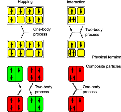
In the following, as we have only considered uniform, periodic superlattices with only nearest neighbour hopping, we will drop the $\mathbf{R}$ labels on the tensor $T$ since it has the same value for all the clusters. In the same vein, the $V$ tensor vanishes for all non-neighbour cluster pairs and takes the same value for all cluster pairs neighbouring in the same orientation. As a result, we shall drop the full $\mathbf{R}\mathbf{R}^{\prime}$ subscript and just subscript it with the neighbouring orientation. For instance, $V_{x}$ denotes the $V$ tensor for clusters neighbouring in the $x$ direction. Similarly to the ZA mapping, which is the one site cluster limit, the body-rank of hopping and on-site interaction terms are swapped. The one-body inter-cluster hopping is mapped into a two-body CFB term involving fermion-boson interactions, while the original two-body on-site interaction is mapped into a sum of one-body composite fermion and one-body composite boson terms. As an illustration, this swapping effect is schematically shown in Figure 1 through an example of an inter-cluster hopping process and an on-site interaction on $2\times 2$ neighbor clusters.

Refer to caption
Figure 1: Schematic representation of an inter-cluster hopping and an on-site interaction processes before (upper part of the figure) and after a mapping to $2\times 2$ composite particles (lower part of the figures). The small yellow squares represent the original lattice sites. Green $2\times 2$ clusters represents CF states, while the red clusters represent CB states. The figure illustrates how a inter-cluster hopping process maps onto a two-body CFB interaction while an on-site two-body interaction maps onto a one-body CB or CF term.

The Hamiltonian (13) is an exact isomorphism of the Hubbard Hamiltonian (12) within the physical subspace of the composite particle Fock space. Although the complexity of the original problem is not reduced, suitable approximations can be carried out with the advantage that short-range quantum correlations are included automatically within the collective structure of the composite particles.

2.2 Mean-field solution

In order to proceed further, we assume that the system is translationally invariant and thus we perform a discrete Fourier transform of the composite operators,

a๐‘โ€‹ฮฑโ€ superscriptsubscript๐‘Ž๐‘๐›ผโ€ \displaystyle a_{\mathbf{R}\alpha}^{{\dagger}} $\displaystyle=$ 1Mโ€‹โˆ‘๐ŠโˆˆBโ€‹Zeโˆ’iโ€‹๐Š๐‘โ€‹a๐Šโ€‹ฮฑโ€ ,1๐‘€subscript๐Š๐ต๐‘superscript๐‘’i๐Š๐‘superscriptsubscript๐‘Ž๐Š๐›ผโ€ \displaystyle\frac{1}{\sqrt{M}}\sum_{\mathbf{K}\in BZ}e^{-{\rm i}\mathbf{K}\mathbf{R}}a_{\mathbf{K}\alpha}^{{\dagger}}, (20)
b๐‘โ€‹ฮฒโ€ superscriptsubscript๐‘๐‘๐›ฝโ€ \displaystyle b_{\mathbf{R}\beta}^{{\dagger}} $\displaystyle=$ 1Mโ€‹โˆ‘๐ŠโˆˆBโ€‹Zeโˆ’iโ€‹๐Š๐‘โ€‹b๐Šโ€‹ฮฒโ€ ,1๐‘€subscript๐Š๐ต๐‘superscript๐‘’i๐Š๐‘superscriptsubscript๐‘๐Š๐›ฝโ€ \displaystyle\frac{1}{\sqrt{M}}\sum_{\mathbf{K}\in BZ}e^{-{\rm i}\mathbf{K}\mathbf{R}}b_{\mathbf{K}\beta}^{{\dagger}}, (21)

where $M$ is the number of sites of the hypercubic superlattice of clusters with size $L^{d}$. The first Brillouin zone ($BZ$) is defined in the interval $(-\pi/L,\pi/L]$ in each direction of the hypercubic reciprocal space. Under this transformation, the Hamiltonian can be written as

$\displaystyle\hat{H}_{CFB}$ $\displaystyle=$ โˆ‘๐Š(Tฮฒโ€ฒฮฒโ€‹b๐Šโ€‹ฮฒโ€ โ€‹b๐Šโ€‹ฮฒโ€ฒ+Tฮฑโ€ฒฮฑโ€‹a๐Šโ€‹ฮฑโ€ โ€‹a๐Šโ€‹ฮฑโ€ฒ)subscript๐Šsuperscriptsubscript๐‘‡superscript๐›ฝโ€ฒ๐›ฝsubscriptsuperscript๐‘โ€ ๐Š๐›ฝsubscript๐‘๐Šsuperscript๐›ฝโ€ฒsuperscriptsubscript๐‘‡superscript๐›ผโ€ฒ๐›ผsubscriptsuperscript๐‘Žโ€ ๐Š๐›ผsubscript๐‘Ž๐Šsuperscript๐›ผโ€ฒ\displaystyle\sum_{\mathbf{K}}\left(T_{\beta^{\prime}}^{\beta}b^{{\dagger}}_{\mathbf{K}\beta}b_{\mathbf{K}\beta^{\prime}}+T_{\alpha^{\prime}}^{\alpha}a^{{\dagger}}_{\mathbf{K}\alpha}a_{\mathbf{K}\alpha^{\prime}}\right) (22)
$\displaystyle+\frac{1}{M}\sum_{u}\sum_{\mathbf{K_{1}K_{2}Q}}\left(V_{u}\right)_{\alpha^{\prime}\beta^{\prime}}^{\beta\alpha}$
ร—(eโˆ’iโ€‹Quโ€‹Lโ€‹b๐Š๐Ÿ,ฮฒโ€ โ€‹a๐Š๐Ÿ+๐,ฮฑโ€ โ€‹a๐Š๐Ÿ+๐,ฮฑโ€ฒโ€‹b๐Š๐Ÿ,ฮฒโ€ฒ+H.c.)absentsuperscript๐‘’isubscript๐‘„๐‘ข๐ฟsuperscriptsubscript๐‘subscript๐Š1๐›ฝโ€ superscriptsubscript๐‘Žsubscript๐Š2๐๐›ผโ€ subscript๐‘Žsubscript๐Š1๐superscript๐›ผโ€ฒsubscript๐‘subscript๐Š2superscript๐›ฝโ€ฒH.c.\displaystyle~{}~{}~{}~{}\times\left(e^{-{\rm i}Q_{u}L}b_{\mathbf{K_{1}},\beta}^{{\dagger}}a_{\mathbf{K_{2}+Q},\alpha}^{{\dagger}}a_{\mathbf{K_{1}+Q},\alpha^{\prime}}b_{\mathbf{K_{2}},\beta^{\prime}}+\text{H.c.}\right)
$\displaystyle+\frac{1}{M}\sum_{u}\sum_{\mathbf{K_{1}K_{2}Q}}\left(V_{u}\right)_{\beta\beta^{\prime}}^{\alpha\alpha^{\prime}}$
ร—(eโˆ’iโ€‹Quโ€‹Lโ€‹a๐Š๐Ÿ,ฮฑโ€ โ€‹a๐Š๐Ÿ+๐,ฮฑโ€ฒโ€ โ€‹b๐Š๐Ÿ+๐,ฮฒโ€‹b๐Š๐Ÿ,ฮฒโ€ฒ+H.c.)absentsuperscript๐‘’isubscript๐‘„๐‘ข๐ฟsuperscriptsubscript๐‘Žsubscript๐Š1๐›ผโ€ superscriptsubscript๐‘Žsubscript๐Š2๐superscript๐›ผโ€ฒโ€ subscript๐‘subscript๐Š1๐๐›ฝsubscript๐‘subscript๐Š2superscript๐›ฝโ€ฒH.c.\displaystyle~{}~{}~{}~{}\times\left(e^{-{\rm i}Q_{u}L}a_{\mathbf{K_{1}},\alpha}^{{\dagger}}a_{\mathbf{K_{2}+Q},\alpha^{\prime}}^{{\dagger}}b_{\mathbf{K_{1}+Q},\beta}b_{\mathbf{K_{2}},\beta^{\prime}}+\text{H.c.}\right)

where repeated Greek indices sum and $\mathbf{K}_{1}$, $\mathbf{K}_{2}$, $\mathbf{K}$, and $\mathbf{Q}$ are summed over all the vectors in the Brillouin zone. $u$ is summed over the spacial dimensions of the system and $V_{u}$ denotes the $V$ tensor for cluster pairs neighbouring in the direction of $u$.

The mean-field treatment of the Hamiltonian (22) assumes a decoupling of the composite fermion and boson spaces, $\ket{\Psi}=\ket{\Psi^{F}}\otimes\ket{\Psi^{B}}$, yielding an effective mean-field Hamiltonian that is quadratic in both the fermionic and bosonic sectors and can be diagonalized by two independent fermionic and bosonic Bogoliubov transformations. The two sectors are coupled via self-consistent boson and fermion mean-fields. In other words, by taking partial variations of the expectation value of $H_{CFB}$ with respect to the fermion and boson wave functions, the stationary condition implies that $\ket{\Psi^{F}}$ and $\ket{\Psi^{B}}$ are eigenfunctions of the effective fermion and boson Hamiltonians,

$\displaystyle\hat{H}^{F}$ $\displaystyle=$ $\displaystyle\bra{\Psi^{B}}\hat{H}_{CFB}\ket{\Psi^{B}},$ (23)
$\displaystyle\hat{H}^{B}$ $\displaystyle=$ $\displaystyle\bra{\Psi^{F}}\hat{H}_{CFB}\ket{\Psi^{F}}.$ (24)

More precisely, the fermionic sector reads

$\displaystyle\hat{H}^{F}$ =โˆ‘๐ŠTฮฑโ€ฒฮฑโ€‹a๐Šโ€‹ฮฑโ€ โ€‹a๐Šโ€‹ฮฑโ€ฒabsentsubscript๐Šsuperscriptsubscript๐‘‡superscript๐›ผโ€ฒ๐›ผsubscriptsuperscript๐‘Žโ€ ๐Š๐›ผsubscript๐‘Ž๐Šsuperscript๐›ผโ€ฒ\displaystyle=\sum_{\mathbf{K}}T_{\alpha^{\prime}}^{\alpha}a^{{\dagger}}_{\mathbf{K}\alpha}a_{\mathbf{K}\alpha^{\prime}}
+1Mโ€‹โˆ‘uโˆ‘๐Š๐(Vu)ฮฑโ€ฒโ€‹ฮฒโ€ฒฮฒโ€‹ฮฑโ€‹(eโˆ’iโ€‹(Kuโˆ’Qu)โ€‹a๐Š,ฮฑโ€ โ€‹a๐Š,ฮฑโ€ฒโ€‹โŸจb๐,ฮฒโ€ โ€‹b๐,ฮฒโ€ฒโŸฉ+H.c.)1๐‘€subscript๐‘ขsubscript๐Š๐superscriptsubscriptsubscript๐‘‰๐‘ขsuperscript๐›ผโ€ฒsuperscript๐›ฝโ€ฒ๐›ฝ๐›ผsuperscript๐‘’isubscript๐พ๐‘ขsubscript๐‘„๐‘ขsuperscriptsubscript๐‘Ž๐Š๐›ผโ€ subscript๐‘Ž๐Šsuperscript๐›ผโ€ฒdelimited-โŸจโŸฉsuperscriptsubscript๐‘๐๐›ฝโ€ subscript๐‘๐superscript๐›ฝโ€ฒH.c.\displaystyle+\frac{1}{M}\sum_{u}\sum_{\mathbf{KQ}}\left(V_{u}\right)_{\alpha^{\prime}\beta^{\prime}}^{\beta\alpha}\left(e^{-{\rm i}(K_{u}-Q_{u})}a_{\mathbf{K},\alpha}^{{\dagger}}a_{\mathbf{K},\alpha^{\prime}}\langle b_{\mathbf{Q},\beta}^{{\dagger}}b_{\mathbf{Q},\beta^{\prime}}\rangle+\text{H.c.}\right)
+1Mโ€‹โˆ‘uโˆ‘๐Š๐(Vu)ฮฒโ€‹ฮฒโ€ฒฮฑโ€‹ฮฑโ€ฒโ€‹(eโˆ’iโ€‹(Kuโˆ’Qu)โ€‹a๐Š,ฮฑโ€ โ€‹aโˆ’๐Š,ฮฑโ€ฒโ€ โ€‹โŸจb๐,ฮฒโ€‹bโˆ’๐,ฮฒโ€ฒโŸฉ+H.c.),1๐‘€subscript๐‘ขsubscript๐Š๐superscriptsubscriptsubscript๐‘‰๐‘ข๐›ฝsuperscript๐›ฝโ€ฒ๐›ผsuperscript๐›ผโ€ฒsuperscript๐‘’isubscript๐พ๐‘ขsubscript๐‘„๐‘ขsuperscriptsubscript๐‘Ž๐Š๐›ผโ€ superscriptsubscript๐‘Ž๐Šsuperscript๐›ผโ€ฒโ€ delimited-โŸจโŸฉsubscript๐‘๐๐›ฝsubscript๐‘๐superscript๐›ฝโ€ฒH.c.\displaystyle+\frac{1}{M}\sum_{u}\sum_{\mathbf{KQ}}\left(V_{u}\right)_{\beta\beta^{\prime}}^{\alpha\alpha^{\prime}}\left(e^{-{\rm i}(K_{u}-Q_{u})}a_{\mathbf{K},\alpha}^{{\dagger}}a_{\mathbf{-K},\alpha^{\prime}}^{{\dagger}}\langle b_{\mathbf{Q},\beta}b_{\mathbf{-Q},\beta^{\prime}}\rangle+\text{H.c.}\right), (25)

and the bosonic sector is obtained by a counterpart mean-field decoupling,

$\displaystyle\hat{H}^{B}$ =โˆ‘๐ŠTฮฒโ€ฒฮฒโ€‹b๐Šโ€‹ฮฒโ€ โ€‹b๐Šโ€‹ฮฒโ€ฒabsentsubscript๐Šsuperscriptsubscript๐‘‡superscript๐›ฝโ€ฒ๐›ฝsubscriptsuperscript๐‘โ€ ๐Š๐›ฝsubscript๐‘๐Šsuperscript๐›ฝโ€ฒ\displaystyle=\sum_{\mathbf{K}}T_{\beta^{\prime}}^{\beta}b^{{\dagger}}_{\mathbf{K}\beta}b_{\mathbf{K}\beta^{\prime}}
+1Mโ€‹โˆ‘uโˆ‘๐Š๐(Vu)ฮฑโ€ฒโ€‹ฮฒโ€ฒฮฒโ€‹ฮฑโ€‹(eโˆ’iโ€‹(Kuโˆ’Qu)โ€‹b๐Š,ฮฒโ€ โ€‹b๐Š,ฮฒโ€ฒโ€‹โŸจa๐,ฮฑโ€ โ€‹a๐,ฮฑโ€ฒโŸฉ+H.c.)1๐‘€subscript๐‘ขsubscript๐Š๐superscriptsubscriptsubscript๐‘‰๐‘ขsuperscript๐›ผโ€ฒsuperscript๐›ฝโ€ฒ๐›ฝ๐›ผsuperscript๐‘’isubscript๐พ๐‘ขsubscript๐‘„๐‘ขsuperscriptsubscript๐‘๐Š๐›ฝโ€ subscript๐‘๐Šsuperscript๐›ฝโ€ฒdelimited-โŸจโŸฉsuperscriptsubscript๐‘Ž๐๐›ผโ€ subscript๐‘Ž๐superscript๐›ผโ€ฒH.c.\displaystyle+\frac{1}{M}\sum_{u}\sum_{\mathbf{KQ}}\left(V_{u}\right)_{\alpha^{\prime}\beta^{\prime}}^{\beta\alpha}\left(e^{-{\rm i}(K_{u}-Q_{u})}b_{\mathbf{K},\beta}^{{\dagger}}b_{\mathbf{K},\beta^{\prime}}\langle a_{\mathbf{Q},\alpha}^{{\dagger}}a_{\mathbf{Q},\alpha^{\prime}}\rangle+\text{H.c.}\right)
+1Mโ€‹โˆ‘uโˆ‘๐Š๐(Vu)ฮฒโ€‹ฮฒโ€ฒฮฑโ€‹ฮฑโ€ฒโ€‹(eโˆ’iโ€‹(Kuโˆ’Qu)โ€‹b๐Š,ฮฒโ€‹bโˆ’๐Š,ฮฒโ€ฒโ€‹โŸจa๐,ฮฑโ€ โ€‹aโˆ’๐,ฮฑโ€ฒโ€ โŸฉ+H.c.).1๐‘€subscript๐‘ขsubscript๐Š๐superscriptsubscriptsubscript๐‘‰๐‘ข๐›ฝsuperscript๐›ฝโ€ฒ๐›ผsuperscript๐›ผโ€ฒsuperscript๐‘’isubscript๐พ๐‘ขsubscript๐‘„๐‘ขsubscript๐‘๐Š๐›ฝsubscript๐‘๐Šsuperscript๐›ฝโ€ฒdelimited-โŸจโŸฉsuperscriptsubscript๐‘Ž๐๐›ผโ€ superscriptsubscript๐‘Ž๐superscript๐›ผโ€ฒโ€ H.c.\displaystyle+\frac{1}{M}\sum_{u}\sum_{\mathbf{KQ}}\left(V_{u}\right)_{\beta\beta^{\prime}}^{\alpha\alpha^{\prime}}\left(e^{-{\rm i}(K_{u}-Q_{u})}b_{\mathbf{K},\beta}b_{\mathbf{-K},\beta^{\prime}}\langle a_{\mathbf{Q},\alpha}^{{\dagger}}a_{\mathbf{-Q},\alpha^{\prime}}^{{\dagger}}\rangle+\text{H.c.}\right). (26)

The physical constraint implies that one-and-only-one state is allowed per cluster, however, the mean-field decoupling of Eqs. (25) and (26) leads to wave functions $\ket{\Psi^{F}}$ and $\ket{\Psi^{B}}$ which do not preserve the local physical constraint (2) exactly. Therefore, we relax it fixing a global constraint of the total composite particle density,

1Mโ€‹โˆ‘๐‘(โˆ‘ฮฑโŸจa๐‘โ€‹ฮฑโ€ โ€‹a๐‘โ€‹ฮฑโŸฉ+โˆ‘ฮฒโŸจb๐‘โ€‹ฮฒโ€ โ€‹b๐‘โ€‹ฮฒโŸฉ)=1.1๐‘€subscript๐‘subscript๐›ผexpectationsubscriptsuperscript๐‘Žโ€ ๐‘๐›ผsubscript๐‘Ž๐‘๐›ผsubscript๐›ฝexpectationsubscriptsuperscript๐‘โ€ ๐‘๐›ฝsubscript๐‘๐‘๐›ฝ1\frac{1}{M}\sum_{\mathbf{R}}\left(\sum_{\alpha}\braket{a^{{\dagger}}_{\mathbf{R}\alpha}a_{\mathbf{R}\alpha}}+\sum_{\beta}\braket{b^{{\dagger}}_{\mathbf{R}\beta}b_{\mathbf{R}\beta}}\right)=1. (27)

This latter condition is added to the effective bosonic and fermionic Hamiltonians via a unique Lagrange multiplier $\lambda$,

$\displaystyle\hat{F}^{F}$ $\displaystyle=$ H^Fโˆ’ฮปโ€‹โˆ‘๐Šโˆ‘ฮฑa๐Šโ€‹ฮฑโ€ โ€‹a๐Šโ€‹ฮฑ,superscript^๐ป๐น๐œ†subscript๐Šsubscript๐›ผsubscriptsuperscript๐‘Žโ€ ๐Š๐›ผsubscript๐‘Ž๐Š๐›ผ\displaystyle\hat{H}^{F}-\lambda\sum_{\mathbf{K}}\sum_{\alpha}a^{{\dagger}}_{\mathbf{K}\alpha}a_{\mathbf{K}\alpha}, (28)
$\displaystyle\hat{F}^{B}$ $\displaystyle=$ H^Bโˆ’ฮปโ€‹โˆ‘๐Šโˆ‘ฮฒb๐Šโ€‹ฮฒโ€ โ€‹b๐Šโ€‹ฮฒ.superscript^๐ป๐ต๐œ†subscript๐Šsubscript๐›ฝsubscriptsuperscript๐‘โ€ ๐Š๐›ฝsubscript๐‘๐Š๐›ฝ\displaystyle\hat{H}^{B}-\lambda\sum_{\mathbf{K}}\sum_{\beta}b^{{\dagger}}_{\mathbf{K}\beta}b_{\mathbf{K}\beta}. (29)

In this work, we have restricted ourselves to wave functions transforming as the totally-symmetric representation of the lattice translation group of the cluster superlattice. We would like to point out that, when the wave function does not break the translational symmetry of the cluster superlattice, the global imposition of the physical constraint would imply local on-average satisfaction of the physical constraint,

โˆ‘ฮฑโŸจa๐‘โ€‹ฮฑโ€ โ€‹a๐‘โ€‹ฮฑโŸฉ+โˆ‘ฮฒโŸจb๐‘โ€‹ฮฒโ€ โ€‹b๐‘โ€‹ฮฒโŸฉ=1,subscript๐›ผexpectationsubscriptsuperscript๐‘Žโ€ ๐‘๐›ผsubscript๐‘Ž๐‘๐›ผsubscript๐›ฝexpectationsubscriptsuperscript๐‘โ€ ๐‘๐›ฝsubscript๐‘๐‘๐›ฝ1\sum_{\alpha}\braket{a^{{\dagger}}_{\mathbf{R}\alpha}a_{\mathbf{R}\alpha}}+\sum_{\beta}\braket{b^{{\dagger}}_{\mathbf{R}\beta}b_{\mathbf{R}\beta}}=1, (30)

for all clusters $\mathbf{R}$. Like in other slave particle approaches, fluctuations of the physical constraint induce mixtures with unphysical states. These unphysical processes are expected to decrease with increasing cluster sizes, approaching the exact physical eigenstate in the infinite size limit, in spite of the combinatorial increase of the computational cost.

In the same vein as our previous composite particle treatment of boson systems [18], one can consider several candidate mean-field reference states. The fermionic part of the product wave function may be treated within a Hartree-Fock (HF) or a Hartree-Fock-Bogoliubov (HFB) approximation, while the bosonic part may be treated within a Hartree-Bose (HB) or a Hartree-Bose-Bogoliubov (HBB) approximation. In this work, we present results for the Hubbard model in one and two dimensions obtained by diagonalizing the fermionic sector via a general HFB transformation, and by treating the bosonic sector in HB and HBB approximations. In the first approximation, we assume that the bosonic sector is described by a coherent state of CBs in the $\mathbf{K=0},~{}\alpha=\sf{c}$ mode, and neglect all bosonic fluctuations (HB). In the second approximation, the bosonic sector is also diagonalized by means of a Bogoliubov transformation (HBB).

Within the coherent approximation, we replace the condensate of CB by a $c-$number b๐ŸŽ,๐–ผ(โ€ )โ†’Mโ€‹ฯƒโ†’subscriptsuperscript๐‘โ€ 0๐–ผ๐‘€๐œŽb^{({\dagger})}_{\mathbf{0},\sf{c}}\rightarrow\sqrt{M}\sigma, where $\sigma^{2}$ is the CB condensate fraction. The coherent CB is a linear combination of CB configurations, i.e., $\ket{\sf{c}}=\sum_{\beta}U^{\sf{c}}_{\beta}\ket{\beta}$. Inserting this transformation into Eq. (29) and minimizing with respect to the variational amplitudes $U^{\sf{c}}$ leads to the Hartree-Bose eigensystem, where $\lambda$ is the lowest eigenvalue, and $U^{\sf{c}}$ its corresponding eigenvector,

$$\sum_{\beta^{\prime}}h^{\mathbf{0},\mathbf{0}}_{\beta\beta^{\prime}}U_{\beta^{\prime}}^{\sf{c}}=\lambda U^{\sf{c}}_{\beta},$$ (31)

where the superindexes of the Hartree matrix $h$ refer to superlattice momentum $\mathbf{K}=\mathbf{0}$. The value of the condensate fraction $\sigma^{2}$ is obtained through the physical constraint,

ฯƒ2=1โˆ’1Mโ€‹โˆ‘๐Šโ€‹ฮฑโŸจa๐Šโ€‹ฮฑโ€ โ€‹a๐Šโ€‹ฮฑโŸฉ.superscript๐œŽ211๐‘€subscript๐Š๐›ผdelimited-โŸจโŸฉsubscriptsuperscript๐‘Žโ€ ๐Š๐›ผsubscript๐‘Ž๐Š๐›ผ\sigma^{2}=1-\frac{1}{M}\sum_{\mathbf{K}\alpha}\langle a^{{\dagger}}_{\mathbf{K}\alpha}a_{\mathbf{K}\alpha}\rangle. (32)

A general symmetry-preserving Bogoliubov transformation for quadratic Hamiltonians has the form [20],

ฮณ๐Šโ€‹ฮท=โˆ‘ฮทโ€ฒ(Xฮทโ€ฒโ€‹ฮท๐Š)โˆ—โ€‹p๐Šโ€‹ฮทโ€ฒโ€ +ฮตโ€‹โˆ‘ฮทโ€ฒ(Yฮทโ€ฒโ€‹ฮทโˆ’๐Š)โˆ—โ€‹pโˆ’๐Šโ€‹ฮทโ€ฒ,subscript๐›พ๐Š๐œ‚subscriptsuperscript๐œ‚โ€ฒsuperscriptsubscriptsuperscript๐‘‹๐Šsuperscript๐œ‚โ€ฒ๐œ‚โˆ—subscriptsuperscript๐‘โ€ ๐Šsuperscript๐œ‚โ€ฒ๐œ€subscriptsuperscript๐œ‚โ€ฒsuperscriptsuperscriptsubscript๐‘Œsuperscript๐œ‚โ€ฒ๐œ‚๐Šsubscript๐‘๐Šsuperscript๐œ‚โ€ฒ\gamma_{\mathbf{K}\eta}=\sum_{\eta^{\prime}}\left(X^{\mathbf{K}}_{\eta^{\prime}\eta}\right)^{\ast}\;p^{{\dagger}}_{\mathbf{K}\eta^{\prime}}+\varepsilon\sum_{\eta^{\prime}}\left(Y_{\eta^{\prime}\eta}^{-\mathbf{K}}\right)^{*}\;p_{\mathbf{-K}\eta^{\prime}}, (33)

where the operators (p๐Šโ€‹ฮทโ€ ,p๐Šโ€‹ฮท)subscriptsuperscript๐‘โ€ ๐Š๐œ‚subscript๐‘๐Š๐œ‚(p^{{\dagger}}_{\mathbf{K}\eta},p_{\mathbf{K}\eta}) refer to fermions $(\varepsilon=+1)$ or bosons $(\varepsilon=-1)$. Accordingly, the $\eta$ labels either CF states $\alpha$ or CB states $\beta$. The amplitudes $X$ and $Y$ are obtained by solving the self-consistent matrix eigensystem of the form [20],

$$\left(\begin{array}[]{cc}h^{\mathbf{K},\mathbf{K}}&\Delta^{\mathbf{K},\mathbf{-K}}\\ \varepsilon(\Delta^{\mathbf{-K},\mathbf{K}})^{*}&\varepsilon(h^{\mathbf{-K},\mathbf{-K}})^{*}\end{array}\right)\left(\begin{array}[]{cc}(X^{\mathbf{K}})^{*}&Y^{\mathbf{K}}\\ (Y^{-\mathbf{K}})^{*}&X^{-\mathbf{K}}\end{array}\right)=\Omega^{\mathbf{K}}\left(\begin{array}[]{cc}(X^{\mathbf{K}})^{*}&Y^{\mathbf{K}}\\ (Y^{-\mathbf{K}})^{*}&X^{-\mathbf{K}}\end{array}\right)$$ (34)

where the positive eigenvalues of the diagonal matrix $\Omega^{\mathbf{K}}=\text{Diag}(-w^{\mathbf{K}},w^{\mathbf{K}})$ will determine the fermionic (bosonic) quasi-particle excitation dispersions. The matrix elements are straightforwardly obtained by identifying the grand-canonical composite particle potentials given in (28) and (29) with the general expression

F^=โˆ‘๐Šโ€‹ฮทโ€‹ฮทโ€ฒ(hฮทโ€‹ฮทโ€ฒ๐Š,๐Šโ€‹p๐Šโ€‹ฮทโ€ โ€‹p๐Šโ€‹ฮทโ€ฒ)+12โ€‹โˆ‘๐Šโ€‹ฮทโ€‹ฮทโ€ฒ(ฮ”ฮทโ€‹ฮทโ€ฒ๐Š,โˆ’๐Šโ€‹p๐Šโ€‹ฮทโ€ โ€‹pโˆ’๐Šโ€‹ฮทโ€ฒโ€ +H.c.)^๐นsubscript๐Š๐œ‚superscript๐œ‚โ€ฒsuperscriptsubscriptโ„Ž๐œ‚superscript๐œ‚โ€ฒ๐Š๐Šsuperscriptsubscript๐‘๐Š๐œ‚โ€ subscript๐‘๐Šsuperscript๐œ‚โ€ฒ12subscript๐Š๐œ‚superscript๐œ‚โ€ฒsuperscriptsubscriptฮ”๐œ‚superscript๐œ‚โ€ฒ๐Š๐Šsubscriptsuperscript๐‘โ€ ๐Š๐œ‚subscriptsuperscript๐‘โ€ ๐Šsuperscript๐œ‚โ€ฒH.c.\hat{F}=\sum_{\mathbf{K}\eta\eta^{\prime}}\left(h_{\eta\eta^{\prime}}^{\mathbf{K},\mathbf{K}}p_{\mathbf{K}\eta}^{{\dagger}}p_{\mathbf{K}\eta^{\prime}}\right)+\frac{1}{2}\sum_{\mathbf{K}\eta\eta^{\prime}}\left(\Delta_{\eta\eta^{\prime}}^{\mathbf{K},\mathbf{-K}}p^{{\dagger}}_{\mathbf{K}\eta}p^{{\dagger}}_{\mathbf{-K}\eta^{\prime}}+\text{H.c.}\right) (35)

The block diagonal structure with respect to $\mathbf{K}$ stems from the fact that all normal density matrix elements โŸจp๐Š1โ€‹ฮทโ€ โ€‹p๐Š2โ€‹ฮทโŸฉexpectationsubscriptsuperscript๐‘โ€ subscript๐Š1๐œ‚subscript๐‘subscript๐Š2๐œ‚\braket{p^{\dagger}_{\mathbf{K}_{1}\eta}p_{\mathbf{K}_{2}\eta}} vanish except for $\mathbf{K}_{1}=\mathbf{K}_{2}$ and the anomalous density matrix elements $\braket{p_{\mathbf{K}_{1}\eta}p_{\mathbf{K}_{2}\eta}}$ vanish except for opposite momentum $\mathbf{K}_{1}=-\mathbf{K}_{2}$ when the wave function transforms according to an irreducible representation of the superlattice translation group. Upon inversion of the Bogoliubov transformation, we obtain the normal and pairing tensors

โŸจp๐Šโ€‹ฮทโ€ โ€‹p๐Šโ€‹ฮทโ€ฒโŸฉdelimited-โŸจโŸฉsubscriptsuperscript๐‘โ€ ๐Š๐œ‚subscript๐‘๐Šsuperscript๐œ‚โ€ฒ\displaystyle\langle p^{{\dagger}}_{\mathbf{K}\eta}p_{\mathbf{K}\eta^{\prime}}\rangle $\displaystyle=$ $\displaystyle\sum_{\zeta}(X^{\mathbf{K}}_{\eta^{\prime}\zeta})^{*}X^{\mathbf{K}}_{\zeta\eta},$ (36)
โŸจp๐Šโ€‹ฮทโ€ โ€‹pโˆ’๐Šโ€‹ฮทโ€ฒโ€ โŸฉdelimited-โŸจโŸฉsubscriptsuperscript๐‘โ€ ๐Š๐œ‚subscriptsuperscript๐‘โ€ ๐Šsuperscript๐œ‚โ€ฒ\displaystyle\langle p^{{\dagger}}_{\mathbf{K}\eta}p^{{\dagger}}_{-\mathbf{K}\eta^{\prime}}\rangle $\displaystyle=$ $\displaystyle-\varepsilon\sum_{\zeta}(Y^{-\mathbf{K}}_{\eta^{\prime}\zeta})^{\ast}X^{\mathbf{K}}_{\zeta\eta}.$ (37)

The convergence of the procedure is determined by the self-consistency between the fermion and boson Hamiltonians and their respective mean-field solutions. In the scheme where we diagonalize both sectors by coupling the fermionic and bosonic Bogoliubov eigensystems self-consistently, the value of the Lagrange multiplier $\lambda$ is varied smoothly until the density of composite particles equals one.

In both of the approximations here considered, the energy of the system can be readily computed taking the expectation value of the CFB Hamiltonian (22) with our ansatz $\ket{\Psi}=\ket{\Psi^{B}}\otimes\ket{\Psi^{F}}$. In particular, for the coherent approximation the total energy reads

$\displaystyle E$ $\displaystyle=$ Mโ€‹T๐–ผ๐–ผโ€‹ฯƒ2+โˆ‘๐ŠTฮฑโ€ฒฮฑโ€‹โŸจa๐Šโ€‹ฮฑโ€ โ€‹a๐Šโ€‹ฮฑโ€ฒโŸฉ๐‘€superscriptsubscript๐‘‡๐–ผ๐–ผsuperscript๐œŽ2subscript๐Šsuperscriptsubscript๐‘‡superscript๐›ผโ€ฒ๐›ผdelimited-โŸจโŸฉsubscriptsuperscript๐‘Žโ€ ๐Š๐›ผsubscript๐‘Ž๐Šsuperscript๐›ผโ€ฒ\displaystyle MT_{\sf c}^{\sf c}\sigma^{2}+\sum_{\mathbf{K}}T_{\alpha^{\prime}}^{\alpha}\langle a^{{\dagger}}_{\mathbf{K}\alpha}a_{\mathbf{K}\alpha^{\prime}}\rangle (38)
+ฯƒ2โ€‹โˆ‘๐Šโˆ‘u(Vu)ฮฑโ€ฒโ€‹๐–ผ๐–ผโ€‹ฮฑโ€‹(eโˆ’iโ€‹Kuโ€‹โŸจa๐Šโ€‹ฮฑโ€ โ€‹a๐Šโ€‹ฮฑโ€ฒโŸฉ+H.c.)superscript๐œŽ2subscript๐Šsubscript๐‘ขsuperscriptsubscriptsubscript๐‘‰๐‘ขsuperscript๐›ผโ€ฒ๐–ผ๐–ผ๐›ผsuperscript๐‘’isubscript๐พ๐‘ขdelimited-โŸจโŸฉsuperscriptsubscript๐‘Ž๐Š๐›ผโ€ subscript๐‘Ž๐Šsuperscript๐›ผโ€ฒH.c.\displaystyle+\sigma^{2}\sum_{\mathbf{K}}\sum_{u}\left(V_{u}\right)_{\alpha^{\prime}{\sf c}}^{{\sf c}\alpha}\left(e^{-{\rm i}K_{u}}\langle a_{\mathbf{K}\alpha}^{{\dagger}}a_{\mathbf{K}\alpha^{\prime}}\rangle+\text{H.c.}\right)
+ฯƒ2โ€‹โˆ‘๐Šโˆ‘u(Vu)๐–ผ๐–ผฮฑโ€‹ฮฑโ€ฒโ€‹(eโˆ’iโ€‹Kuโ€‹โŸจa๐Šโ€‹ฮฑโ€ โ€‹aโˆ’๐Šโ€‹ฮฑโ€ฒโ€ โŸฉ+H.c.).superscript๐œŽ2subscript๐Šsubscript๐‘ขsuperscriptsubscriptsubscript๐‘‰๐‘ข๐–ผ๐–ผ๐›ผsuperscript๐›ผโ€ฒsuperscript๐‘’isubscript๐พ๐‘ขdelimited-โŸจโŸฉsuperscriptsubscript๐‘Ž๐Š๐›ผโ€ superscriptsubscript๐‘Ž๐Šsuperscript๐›ผโ€ฒโ€ H.c.\displaystyle+\sigma^{2}\sum_{\mathbf{K}}\sum_{u}\left(V_{u}\right)_{\sf cc}^{\alpha\alpha^{\prime}}\left(e^{-{\rm i}K_{u}}\langle a_{\mathbf{K}\alpha}^{{\dagger}}a_{\mathbf{-K}\alpha^{\prime}}^{{\dagger}}\rangle+\text{H.c.}\right).

where repeated indices are summed and we have performed a contraction of the original tensors $T$ and $V$ with the boson condensate $\sf{c}$. Notice that, as the mean-field treatment does not preserve the physical constraint exactly, the energy reached is not an upper bound to the exact ground state energy. Nevertheless, by performing a finite-size scaling analysis one can give a quantitative estimate of the exact result.

We are also interested in the double-occupation parameter, which gives a measure of on-site physical fermion correlations and provides a qualitative indicator of the Mott insulator transition. It is here computed in the CFB mean-field approximations as

Dj=โŸจnjโ†“โ€‹njโ†‘โŸฉ=โˆ‘ฮฒโŸจ๐‘โ€‹ฮฒ|โ€‹njโ†‘โ€‹njโ†“โ€‹|๐‘โ€‹ฮฒโŸฉโ€‹โŸจb๐‘โ€‹ฮฒโ€ โ€‹b๐‘โ€‹ฮฒโŸฉ+โˆ‘ฮฑโŸจ๐‘โ€‹ฮฑ|โ€‹njโ†‘โ€‹njโ†“โ€‹|๐‘โ€‹ฮฑโŸฉโ€‹โŸจa๐‘โ€‹ฮฑโ€ โ€‹a๐‘โ€‹ฮฑโŸฉ,subscript๐ท๐‘—delimited-โŸจโŸฉsubscript๐‘›โ†“๐‘—absentsubscript๐‘›โ†‘๐‘—absentsubscript๐›ฝbra๐‘๐›ฝsubscript๐‘›โ†‘๐‘—absentsubscript๐‘›โ†“๐‘—absentket๐‘๐›ฝdelimited-โŸจโŸฉsubscriptsuperscript๐‘โ€ ๐‘๐›ฝsubscript๐‘๐‘๐›ฝsubscript๐›ผbra๐‘๐›ผsubscript๐‘›โ†‘๐‘—absentsubscript๐‘›โ†“๐‘—absentket๐‘๐›ผdelimited-โŸจโŸฉsubscriptsuperscript๐‘Žโ€ ๐‘๐›ผsubscript๐‘Ž๐‘๐›ผD_{j}=\langle n_{j\downarrow}n_{j\uparrow}\rangle=\sum_{\beta}\bra{\mathbf{R}\beta}n_{j\uparrow}n_{j\downarrow}\ket{\mathbf{R}\beta}\langle b^{{\dagger}}_{\mathbf{R}\beta}b_{\mathbf{R}\beta}\rangle+\sum_{\alpha}\bra{\mathbf{R}\alpha}n_{j\uparrow}n_{j\downarrow}\ket{\mathbf{R}\alpha}\langle a^{{\dagger}}_{\mathbf{R}\alpha}a_{\mathbf{R}\alpha}\rangle, (39)

with $j\in\mathbf{R}$.

As a short recapitulation, we have presented a canonical mapping which allows us to express a many-fermion lattice Hamiltonian as a many fermion-boson system on a superlattice of clusters. The composite boson and fermion cluster operators contain the exact quantum correlations inside the clusters. In order for the mapping to be an exact isomorphism, a physical constraint has to be satisfied. We proposed a mean-field ansatz for our mapped Hamiltonian that is a direct product of fermionic and bosonic states that preserve the superlattice translational symmetry. In the following, we present results obtained with this approach.

3 Results and discussion

Refer to caption
Refer to caption
Figure 2: Ground state energies per site and double-occupancies of the 1-D Hubbard model obtained from the CFB mean-field theory with various clusters sizes ($L=2,4,6$), the restricted and unrestricted Hartree-Fock (HF) approximation, and the exact Bethe anstaz (BA). The insets amplifies the differences in particular coupling regimes $U$.

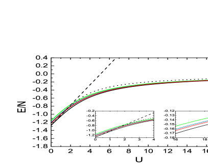
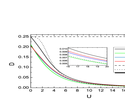
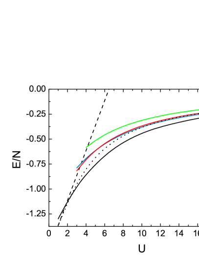
We start the numerical analysis of the method by studying the ground-state energy $E$ (38) and double-occupation $D$ (39) of the Hubbard model at half-filling (12) by means of the HB approximation for the CB Hamiltonian (29), and HFB for the CF Hamiltonian (28). Half-filling can be achieved by setting the chemical potential $\mu$ to half the value of the Hubbard repulsion parameter $U$ for particle-hole symmetry. In Figure 2, we present the energy per site (left panel) and double-occupation (right panel) for various values of $U$. We also include the exact energy per site obtained by the Bethe ansatz [1] and the energy obtained by both the standard, symmetry-preserving and the unrestricted HF approximations of the original Hubbard Hamiltonian (12). The RHF mean-field methods is exact in the non-interacting limit, $U=0$; however, it quickly deteriorates with increasing interaction. The ground state energy obtained with the CFB mean-field is in very good agreement with the exact result for large $U$. The UHF method is able to provide a qualitatively reasonable result for both small and large $U$. So it parallels the trend for the Bethe ansatz, but becomes higher in energy than the CFB mean-field energy for larger $U$ values. The right inset shows how the CFB mean-field energy converges to the exact one as the size of the cluster is increased. In this way, a significant portion of the correlation energy relative to the RHF solution can be captured. However, at low $U$, the energy from the CFB mean-field theory starts to deviate from the exact Bethe ansatz value, and crosses the RHF energy at $U\sim 1.4$ for the size-six cluster, as it can be seen in the left inset.

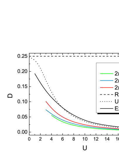
By inspecting the double-occupation expectation value (39) shown in the right panel of Figure 2, we check that the method becomes more accurate for intermediate and strong repulsion by increasing the size of the cluster (see right panel inset). The deviation at weak coupling can in fact be understood by a careful scrutiny of the method and its strengths. The kinetic and interacting terms of the Hubbard Hamiltonian (12) are one- and two-body terms, respectively, when written in terms of the physical fermions. In the mapped Hamiltonian (13) part of the kinetic term is computed in mean-field (inter-cluster contribution) and part is computed exactly (intra-cluster contribution), while the on-site interaction is always computed exactly. As a result, when minimizing the effective mean-field energy, the CFB mean-field tends to underestimate the kinetic contribution, leading to a wave function with low double-occupancy at the expense of a higher kinetic energy. By increasing the cluster size, we are including more hopping processes into the exact computation. In this way, the method is able to yield lower total energy by lowering the kinetic energy and adjusting the double-occupancy to higher values. This trend is exactly analogous to mean-field theory of physical fermions, where the HF method lowers the one-particle kinetic energy to a large extent but yields too high a repulsion energy and thus non-optimal total energy. In this way, it can be seen that the CFB mean-field theory is highly complementary to the mean-field theory based on physical fermions because they are treating different terms in a mean-field way. The physical fermion mean-field theory performs better in the small $U$ regime, like in the Fermi-liquid phase, while the fermion-boson mean-field theory performs better in large $U$ regimes like the Mott insulating phase. Also apparent in this figure is the systematic improvement of the method when the size of the cluster is increased.

Refer to caption
Refer to caption
Figure 3: Ground state energy per site versus the inverse of the clusters size $L$ for the CFB approximations and exact diagonalization showing the convergence to the exact Bethe ansatz value at intermediate ($U=4$) and strong ($U=8$) Hubbard interactions.

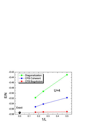
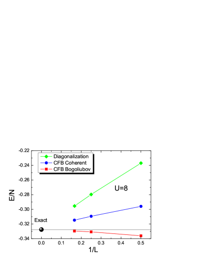
In Figure 3 we show the convergence of the energy per site towards the exact Bethe ansatz result as a function of the reciprocal of the number of sites in the cluster, $1/L$, for $U=4$ in the left panel and $U=8$ in the right panel. Specifically we depict the energy of a single isolated cluster obtained from exact diagonalization of $\hat{H}_{R}^{\square}$, together with the two CFB mean-field treatments described above: the bosonic coherent wave function (CFB Coherent) and the bosonic Bogoliubov wave function (CFB Bogoliubov). A clear improvement of the energy is seen in both panels as a function of $1/L$. In the limit where the cluster becomes the entire system, inter-cluster processes, which are here treated approximately in mean-field, are no longer present, the CFB Hamiltonian becomes doubly quadratic and represents the even and odd number parity sectors of the exact Hamiltonian. As a result, CFB mean-field becomes exact in this limit and simply corresponds to picking the exact ground state as the composite particle to occupy. As seen in Figure 3, in both approaches (Coherent and Bogoliubov), the energy extrapolates to the exact result. The CFB Bogoliubov treatment adds bosonic fluctuations to the coherent-state approximation. The improvement is apparent in the figure, despite the fact that for strong coupling ($U=8$) the method overbinds. This is due to violations of the physical constraint (2) when treated on average (30), that induces mixtures with unphysical states, a point that will be addressed in future works. Notice that the computational cost associated with increasing the cluster size is combinatorial, limiting the size of clusters that can be used as building blocks for the mapping. An alternative way to improve the precision of the method is the use of more sophisticated many-body approaches to treat the CFB Hamiltonian (13).

We have also applied the CFB mean-field approach within the coherent approximation to the two-dimensional Hubbard model at half filling. Results for the ground state energies and double-occupancies are displayed in figure 4 using clusters of sizes $2\times 1$, $2\times 2$, and $2\times 3$. We have been unable to reach a self-consistent solution for small $U$ values, even with sophisticated convergence-acceleration techniques [21]. This might stem from the fact that larger spatial dimensionality implies larger weight of the kinetic energy term in the Hamiltonian. In this sense, when a larger part of the Hamiltonian is treated in mean-field, convergence can be harder to achieve. The two-dimensional Hubbard model exhibits antiferromagnetic (AF) long-range order for all repulsive $U$ [22]. Inspecting our converged density matrix for the $2\times 2$ cluster, we find that one of the two possible AF boson states gets a significantly larger weight than the other. This symmetry breaking cannot be observed in the $2\times 1$ and $2\times 3$ cases because these lattices are not commensurate with AF long-range ordering. This observation rationalizes the significant energy difference between them and the reported relatively high stability of the $2\times 2$ case. Also the symmetry-breaking has not been observed for the one-dimensional model, as expected.

A noticeable difference between the one-dimensional and two-dimensional cases is the relative energy between the CFB mean-field theory and HF of physical fermions. In 1D systems, starting from $U=1.4$ for the size-six cluster, $U=1.7$ for size-four cluster, and $U=2.2$ for size-two cluster, HF yields a lower ground-state energy than the composite mean-field approach. We can take this $U$ crossover ratios as a rough estimate of the Mott transition point, which the exact solution predicts at $U=0$ [1]. In the two-dimensional problem, recent DMFT results [23] place the Mott-insulator transition at approximately $U=5.3$. This is slightly higher than the crossing points between HF and our composite mean-field results.

Refer to caption
Refer to caption
Figure 4: Ground state energies per site and double-occupancies of the 2-D Hubbard model obtained from the CFB mean-field theory with various clusters sizes, from the restricted and unrestricted Hartree-Fock approximation, and from an exact diagonalization of an isolated $4\times 4$ cluster.

4 Conclusion

In this work, we have proposed a mapping of fermion operators onto composite fermion and boson cluster operators in one-to-one correspondence to many-electron states. The mapping was used to transform the standard Hubbard model onto a new composite fermion-boson Hamiltonian acting on a cluster superlattice that can be treated by standard many-body approximations. The advantage of the cluster mapping is that the short-range interactions and the local quantum fluctuations are taken into account exactly from the onset. Specifically, on-site interactions and intra-cluster hopping processes are computed exactly by definition.

We have proposed a mean-field ansatz built as a tensor product of a fermionic and bosonic wave function. This ansatz in terms of composite particles can exactly handle single-cluster operators (such as the on-site repulsion), while inter-cluster scattering processes (such as hopping) are treated in a mean-field way. We showed that the ansatz performs well for large $U$ at half-filling, and is fairly complementary to the Hartreeโ€“Fock approach of physical fermions, which treats hopping exactly at the expense of only a mean-field treatment of the on-site repulsion interaction. We plan to explore, in future work, the applicability of the ansatz to the doped phases of the Hubbard Hamiltonian.

5 Acknowledgments

This work was supported by the Department of Energy, Office of Basic Energy Sciences, Grant No. DE-FG02-09ER16053, the Welch Foundation (C-0036), DOE-CMCSN (DESC0006650), and by the Spanish Ministry of Economy and Competitiveness trough grants FIS2012-34479 and BES-2010-031607.

References

References

  • [1] E.ย H. Lieb and F.ย Y. Wu. Absence of Mott transition in an exact solution of the short-range, one-band model in one dimension. Phys. Rev. Lett., 20:1445โ€“1448, 1968.
  • [2] S.ย Zhang, J.ย Carlson, and J.ย E. Gubernatis. Pairing correlations in the two-dimensional Hubbard model. Phys. Rev. Lett., 78:4486โ€“4489, 1997.
  • [3] M.ย Guerrero, G.ย Ortiz, and J.ย E. Gubernatis. Correlated wave functions and the absence of long-range order in numerical studies of the hubbard model. Phys. Rev. B, 59:1706โ€“1711, 1999.
  • [4] S.ย Sorella. Wave function optimization in the variational Monte Carlo method. Phys. Rev. B, 71:241103, 2005.
  • [5] A.ย Georges, G.ย Kotliar, W.ย Krauth, and M.ย J. Rozenberg. Dynamical mean-field theory of strongly correlated fermion systems and the limit of infinite dimensions. Rev. Mod. Phys., 68:13โ€“125, 1996.
  • [6] U.ย Schollwรถck. The density-matrix renormalization group. Rev. Mod. Phys., 77:259โ€“315, 2005.
  • [7] G.ย Knizia and G.ย K.-L. Chan. Density matrix embedding: A simple alternative to dynamical mean-field theory. Phys. Rev. Lett., 109:186404, 2012.
  • [8] I.ย W. Bulik, G.ย E. Scuseria, and J.ย Dukelsky. Density matrix embedding from broken symmetry lattice mean fields. Phys. Rev. B, 89:035140, 2014.
  • [9] G.ย Kotliar, S.ย Y. Savrasov, G.ย Pรกlsson, and G.ย Biroli. Cellular dynamical mean field approach to strongly correlated systems. Phys. Rev. Lett., 87:186401, 2001.
  • [10] M.ย Balzer, W.ย Hanke, and M.ย Potthoff. Mott transition in one dimension: Benchmarking dynamical cluster approaches. Phys. Rev. B, 77:045133, 2008.
  • [11] G.ย Kotliar and A.ย E. Ruckenstein. New functional integral approach to strongly correlated fermi systems: The Gutzwiller approximation as a saddle point. Phys. Rev. Lett., 57:1362โ€“1365, 1986.
  • [12] Z.ย Zou and P.ย W. Anderson. Neutral fermion charge-e boson excitations in the resonating-valence-bond state and superconductivity in La2CnO4-based compounds. Phys. Rev. B, 37:627, 1988.
  • [13] S.ย ร–stlund and M.ย Granath. Exact transformation for spin-charge separation of spin-$1/2$ fermions without constraints. Phys. Rev. Lett., 96:066404, 2006.
  • [14] P.ย A. Lee, N.ย Nagaosa, and X.-G. Wen. Doping a Mott insulator: Physics of high-temperature superconductivity. Rev. Mod. Phys., 78:17โ€“85, 2006.
  • [15] K.ย Scharnhorst and J.-W. van Holten. Nonlinear Bogolyubov-Valatin transformations: Two modes. Ann. Phys., 326(11):2868 โ€“ 2933, 2011.
  • [16] P.ย Ribeiro, P.D. Sacramento, and M.A.N. Araรบjo. U(1) slave-particle study of the finite-temperature doped Hubbard model in one and two dimensions. Ann. Phys., 326:1189โ€“1206, 2011.
  • [17] L.ย Isaev, G.ย Ortiz, and J.ย Dukelsky. Hierarchical mean-field approach to the ${J}_{1}-{J}_{2}$ Heisenberg model on a square lattice. Phys. Rev. B, 79:024409, 2009.
  • [18] D.ย Huerga, J.ย Dukelsky, and G.ย E. Scuseria. Composite boson mapping for lattice boson systems. Phys. Rev. Lett., 111:045701, 2013.
  • [19] E.ย Altman and A.ย Auerbach. Plaquette boson-fermion model of cuprates. Phys. Rev. B, 65:104508, 2002.
  • [20] J.-P. Blaizot and G.ย Ripka. Quantum Theory of Finite Systems. The MIT Press, Cambridge, MA, 1986.
  • [21] P.ย Pulay. Improved SCF convergence acceleration. J. Comput. Chem., 3:556โ€“560, 1982.
  • [22] J.ย E. Hirsch and S.ย Tang. Antiferromagnetism in the two-dimensional Hubbard model. Phys. Rev. Lett., 62:591โ€“594, 1989.
  • [23] G.ย Sordi, K.ย Haule, and A.-M.ย S. Tremblay. Mott physics and first-order transition between two metals in the normal-state phase diagram of the two-dimensional Hubbard model. Phys. Rev. B, 84:075161, 2011.