Topology and Self-Similarity of the Hofstadter Butterfly

Abstract

We revisit the problem of self-similar properties of the Hofstadter butterfly spectrum, focusing on spectral as well as topological characteristics. In our studies involving any value of magnetic flux and arbitrary flux interval, we single out the most dominant hierarchy in the spectrum, which is found to be associated with an irrational number $\zeta=2+\sqrt{3}$ where nested set of butterflies describe a kaleidoscope. Characterizing an intrinsic frustration at smallest energy scale, this hidden quasicrystal encodes hierarchical set of topological quantum numbers associated with Hall conductivity and their scaling properties. This topological hierarchy maps to an integral Apollonian gasket near-$D_{3}$ symmetry, revealing a hidden symmetry of the butterfly as the energy and the magnetic flux intervals shrink to zero. With a periodic drive that induces phase transitions in the system, the fine structure of the butterfly is shown to be amplified making states with large topological invariants accessible experimentally.

I Introduction

Hofstadter butterflyHofstadter (1976), also known as GplotHopstadter (1989) is a fascinating two-dimensional spectral landscape, a quantum fractal where energy gaps encode topological quantum numbers associated with the Hall conductivityThouless et al. (1982). This intricate mix of order and complexity is due to frustration, induced by two competing periodicities as electrons in a crystalline lattice are subjected to a magnetic field. The allowed energies of the electrons are discontinuous function of the magnetic flux penetrating the unit cell, while the gaps , the forbidden energies are continuous except at discrete points. The smoothness of spectral gaps in this quantum fractal may be traced to topology which makes spectral properties stable with respect to small fluctuations in the magnetic flux when Fermi energy resides in the gap. The Gplot continues to arouse a great deal of excitement since its discovery, and there are various recent attempts to capture this iconic spectrum in laboratoryDean et al. (2013); Aidelsburger et al. (2013); Weld et al. (2013).

Fractal properties of the butterfly spectrum have been the subject of various theoretical studiesWannier (1978); MacDonald (1983); Wilkinson (1987, 1994); Chang and Niu (1996); MacDonald (2009). However, detailed description quantifying self-similar universal properties of the butterfly and the universal fixed point butterfly function has not been reported previously. In contrast to earlier studies where self-similarity of the spectrum is studied for a fixed value of the magnetic flux such as the golden-mean, and thus focusing on certain isolated local parts of the spectrum, this paper presents self-similar butterfly that is reproduced at all scales in magnetic flux.

In this paper, we address following questions regarding the butterfly fractal: (1) How to describe self-similar fractal properties of the butterfly at any value of magnetic flux given arbitrary flux interval. We determine the recursion relation, for determining the magnetic flux interval from one generation to the next , so that one reproduces the entire butterfly structure . In other words, we seek the fixed point function that contains the entire Gplot as the magnetic flux and the energy scales shrinks to zero. We try to answer this question without confining to a specific magnetic flux value such as the golden-mean and obtain universal scaling and the fixed point butterfly function that describes the spectrum globally. (2) In addition to spectral scaling, we also address the question of scaling for the topological quantum numbers . (3) We briefly investigate butterfly fractal for special values of magnetic flux such as the golden and the silver-mean that has been the subject of almost all previous studies. (4) Finally, we present a mechanism for amplifying small gaps of the butterfly fractal, making them more accessible in laboratory.

Our approach here is partly geometrical and partially numerical. Using simple geometrical and number theoretical tools, we obtain the exact scaling associated with the magnetic flux interval. Here we address the question of both magnetic flux as well as topological scaling. The spectral gaps are labeled by two quantum numbers which we denote as $\sigma$ and $\tau$. The integer $\sigma$ is the Chern number , the quantum number associated with Hall conductivityThouless et al. (1982) and $\tau$ is an integer. These quantum numbers satisfy the Diophantine equation (DE)Dana I (1985),

$$\rho=\phi\sigma+\tau$$ (1)

where $\rho$ is the particle density when Fermi level is in the gap and $\phi$ denotes the magnetic flux per unit cell. We obtain exact expressions describing scaling of these quantum numbers in the butterfly hierarchy. The spectral scaling describing universal scalings associated with the energy interval is obtained numerically. Our analysis is mostly confined to the energy scales near $E=0$, that is near half-filling. This is a reasonable choice for two reasons: firstly, simple observation of the butterfly spectrum shows gaps of the spectrum forming $4$-wing structures ( the butterflies) exist mostly near half-filling. Secondly, gaps away from half-filling appear to be continuation of the gaps that exist near $E=0$. We believe that although the gaps characterized by a fixed $(\sigma\tau)$ are discontinuous at rational values of the flux, , these gaps continue ( with same topological numbers ) after a break at rational flux values, with their derivatives w.r.t the magnetic flux continuous

I.1 Summary of the main results

• Given an arbitrary value of magnetic flux $\phi_{0}$ and an arbitrary flux interval $\delta\phi$, (no matter how small), there is a precise rule for obtaining the entire butterfly in that interval, as described in section (3-A).

• Simple number theory provides an exact scaling ratio between two successive generations of the butterfly and this scaling is universal, independent of the initial window for zooming , described in subsections (3-B) and (IV).

• The hierarchy characterized by the irrational numbers whose tail exhibit period-$2$ continued fraction expansion with entries $1$ and $2$ , which we denote as $\zeta_{1,2}$ emerges as the most ”dominant” hierarchy as is associated with the smallest scaling ratio that describes butterflies between two successive generations. Commonly studied hierarchies characterized by golden-tail, which we denote as $\zeta_{1}$ ( set of irrationals who tail end exhibits integer $1$ only in its continued fraction expanding) are of lower significance as they are characterized by larger scaling ratio. A comparison between different hierarchies is given in Table III.

• The emergence of $\zeta_{1,2}$ class of irrationals with the universal butterfly and its topological hierarchy of quantum numbers reveals a hidden dodecagonal quasicrystalline symmetryMacDonald (1989) in the butterfly spectrum. These results also apply to other lattices such as graphene in a magnetic field.

• The dominant hierarchy $\zeta_{1,2}$ maps to a geometrical fractal known as the Integral Apollonian gasketMandelbrot (1982) that asymptotically exhibits near $D_{3}$ symmetry and the nested set of butterflies describe a kaleidoscope where two successive generations of butterfly are mirror images through a circular mirror. This is discussed in section V.

• In our investigation of the fractal properties of the Hofstadter butterfly, one of the key guiding concepts is a corollary of the DE equation that quantifies the topology of the fine structure near rational fluxes . We show that, for every rational flux, an infinity of possible solutions of the DE, although not supported in the simple square lattice model , are present in close vicinity of the flux. ( See section (IV)). Consequently, perturbations that induce topological phase transitions can transform tiny gaps with large topological quantum numbers into major gaps. This might facilitate the creation of such states in an experimental setting. In section VII, we illustrate this amplification by periodically driving the system.

II Model System and Topological Invariants

Model system we study here consists of (spinless) fermions in a square lattice. Each site is labeled by a vector ${\bf r}=n\hat{x}+m\hat{y}$, where $n$, $m$ are integers, $\hat{x}$ ($\hat{y}$) is the unit vector in the $x$ ($y$) direction, and $a$ is the lattice spacing. The tight binding Hamiltonian has the form

$$H=-J_{x}\sum_{\bf r}|\mathbf{r}+\hat{x}\rangle\langle\mathbf{r}|-J_{y}\sum_{\bf r}|\mathbf{r}+\hat{y}\rangle e^{i2\pi n\phi}\langle\mathbf{r}|+h.c.$$ (2)

Here, $|\mathbf{r}\rangle$ is the Wannier state localized at site $\mathbf{r}$. $J_{x}$ ($J_{y}$) is the nearest neighbor hopping along the $x$ ($y$) direction. With a uniform magnetic field $B$ along the $z$ direction, the flux per plaquette, in units of the flux quantum $\Phi_{0}$, is $\phi=-Ba^{2}/\Phi_{0}$.

In the Landau gauge realized in experimentsLin et al. (2009), the vector potential $A_{x}=0$ and $A_{y}=-\phi x$, the Hamiltonian is cyclic in $y$ so the eigenstates of the system can be written as $\Psi_{n,m}=e^{ik_{y}m}\psi_{n}$ where $\psi_{n}$ satisfies the Harper equationHarper (1955)

$$e^{ik_{x}}\psi^{r}_{n+1}+e^{-ik_{x}}\psi^{r}_{n-1}+2\lambda\cos(2\pi n\phi+k_{y})\psi^{r}_{n}=E\psi^{r}_{n}.$$ (3)

Here $n$ ($m$) is the site index along the $x$ ($y$) direction, $\lambda=J_{y}/J_{x}$ and $\psi^{r}_{n+q}=\psi^{r}_{n}$, $r=1,2,...q$ are linearly independent solutions. In this gauge the magnetic Brillouin zone is $-\pi/qa\leq k_{x}\leq\pi/qa$ and $-\pi\leq k_{y}\leq\pi$.

At flux $\phi=p/q$, the energy spectrum has in general $q-1$ gaps. For Fermi level inside each energy gap, the system is in an integer quantum Hall stateThouless et al. (1982) characterized by its Chern number $\sigma$, the quantum number associated with the transverse conductivity $C_{xy}=\sigma{e^{2}}/{h}$Thouless et al. (1982). The $\sigma$ and $\tau$ are two quantum numbers that label various gaps of the butterfly and are solutions of DEDana I (1985). The possible values of these integers are,

$$(\sigma,\tau)=(\sigma_{0}-nq,\tau_{0}+np)$$ (4)

Here $\sigma_{0},\tau_{0}$ are any two integers that satisfy the Eq. (1) and $n$ is an integer. The quantum numbers $\sigma$ that determines the quantized Hall conductivity corresponds to the change in density of states when the magnetic flux quanta in the system is increased by one and whereas the quantum number $\tau$ is the change in density of states when the period of the potential is changed so that there is one more unit cell in the system.

For any value of the magnetic flux , the system described by the Hamiltonian (2), supports only $n=0$ solution of Eq. (4) for the quantum numbers $\sigma$ and $\tau$. Absence of changes in topological states from $n=0$ to higher $n$ values is due to the absence of any gap closing and reopening that is essential for any topological phase transition. However, as shown later, the DE which relates continuously varying quantities $\rho$ and $\phi$ with integers $\sigma$ and $\tau$, has some important consequences about topological changes in close vicinity of rational values of $\phi$.

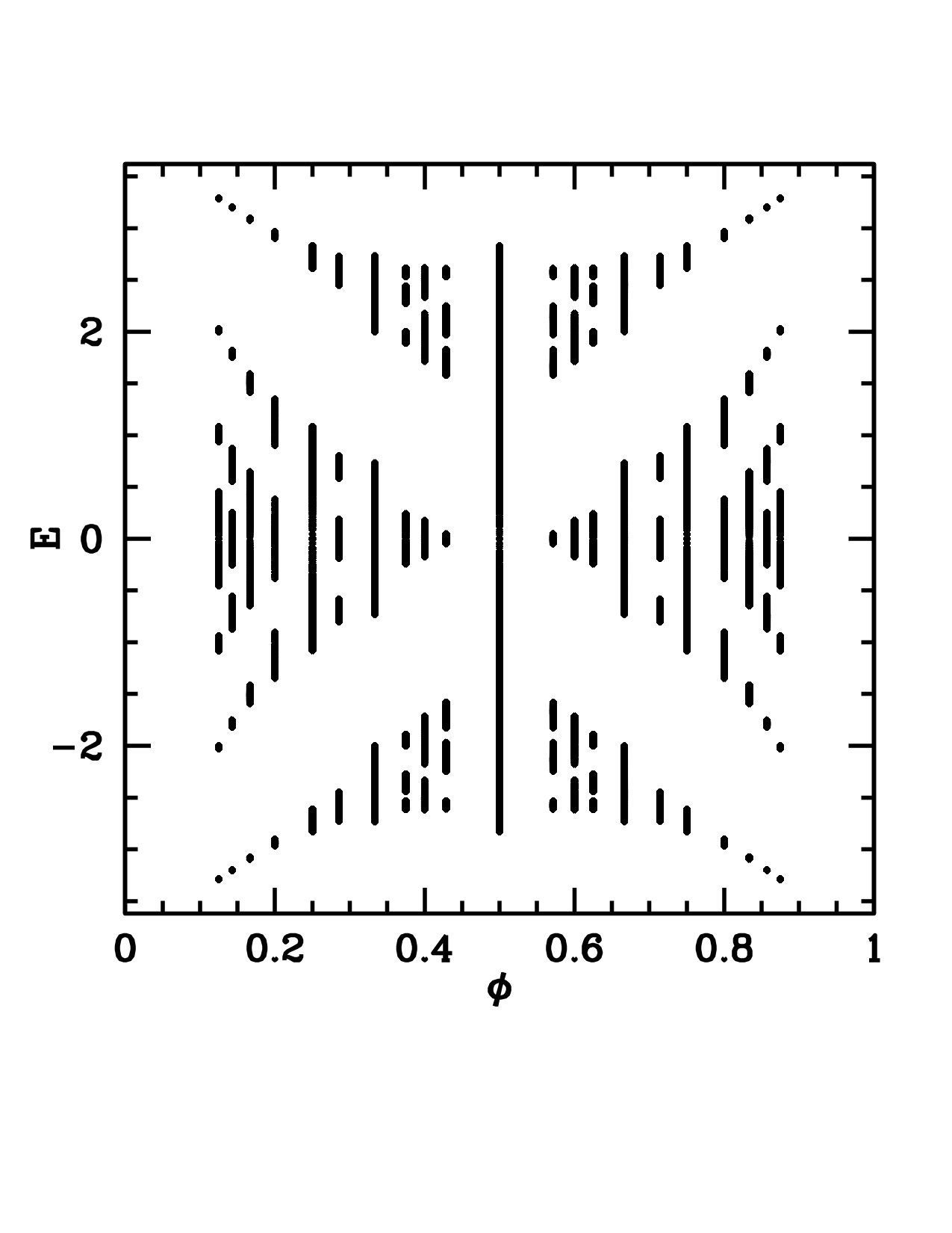
Figure 1: Figure shows the butterfly graph for values of $\phi=p/q$ with $q_{max}=8$. For fixed $p/q$, the energy ( vertical axis) shows $q$ bands and $q-1$ gaps for odd-$q$ case. For $q$-even, the two bands at the center touch and therefore there are only $q-2$ gaps.

Figure 2: Graphs highlight the distinction between the even and the odd-denominator flux values by showing the central band of the butterfly spectrum in the immediate neighborhood of $\phi=1/4$ ( left) and $\phi=1/3$ ( right). This illustrates typical scenario where near even denominator fractions the fragmented band structure clusters into two distinct bands, touching at the center while for the odd-denominator fractions, the fragmented structure clusters around a single band.

III Butterfly Fractal

III.1 Miniature Copies of the Butterfly Graph: Butterfly at Every Scale

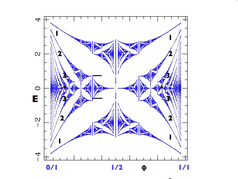
Figure 3: (color on line) Level-$1$ butterfly in $\phi$ intervals $[1/3-2/5]$ where the horizontal bars show the $\phi$-interval that is zoomed in the level-$2$. The magnitude of the Chern numbers for the central butterfly and its left and right harmonics are $1+3n$ and $|1-5n|$, $n=1,2,3..$ as shown are determined using DE equation.

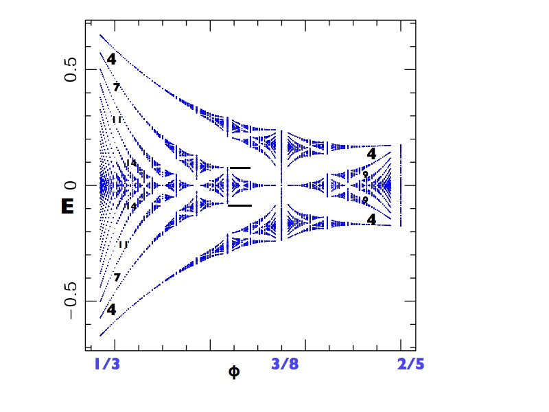
Figure 4: (color on line) Level-$1$ butterfly in $\phi$ intervals $[1/3-2/5]$ where the horizontal bars show the $\phi$-interval that is zoomed in the level-$2$. The magnitude of the Chern numbers for the central butterfly and its left and right harmonics are $1+3n$ and $|1-5n|$, $n=1,2,3..$ as shown.

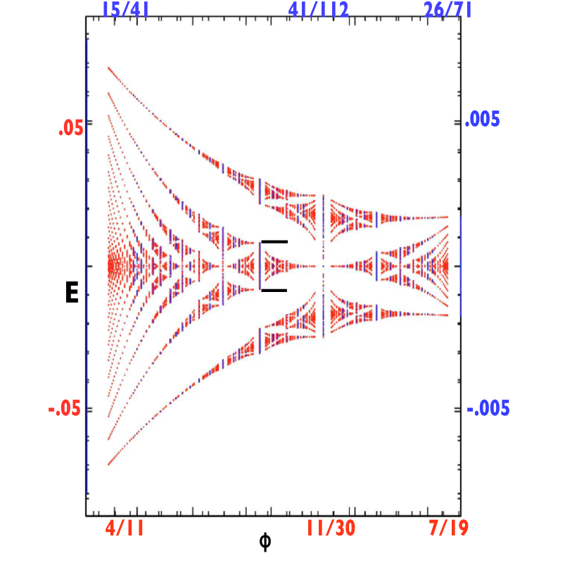
Figure 5: (color on line) Figure displays an overlay of level-$2$ and level $3$ butterflies in $\phi$ intervals $[4/11,7/19]$ and $[15/41,26/71]$ giving energy scale ratio $\approx 10$ as shown in red and blue respectively. The magnetic flux scaling is found to be $\zeta^{2}$ as described later. This illustrates an approach to fixed point butterfly fractal as $E$ and $\phi$ intervals shrink to zero. Note that the $\phi$ scale is shown only at the boundaries and the centers of the butterflies. The magnitude of topological numbers for the central butterflies for level-$2$ and $3$ are respectively given by $(15,3)$ and $(56,20)$. The asymmetry of the butterfly about its center reflects the asymmetry in the Chern numbers of the left and the right harmonics which can be determined from Eq. (21).

Butterfly graph is a plot of possible energies of the electron for various values of $\phi$ which varies between $[0,1]$. To understand this graph, we begin with values of $\phi$ that are rational numbers, focusing on simple fractions. Figure (1) shows one such graph, a skeleton of the butterfly graph, obtained using few rational values. The permissible energies are arranged in bands separated from forbidden values, the gaps. In general, for a fixed $\phi=\frac{p}{q}$, the graph consists of of $q$ bands ( the dark regions) and $(q-1)$ gaps ( empty regions).

For $q$-even, the two central bands touch one another and therefore, we see only $(q-2)$ gaps. The graphs show important distinctions between the even and the odd-denominator fractions as shown in Fig.(2). As we look in the immediate vicinity of even-denominator flux values, the two touching bands begin to split, opening a gap at the center. Consequently, in the butterfly landscape, as we look both to the left and to the right of the even-denominator fraction, we see four gaps or swaths resembling the four-wings of a butterfly, all converging at the center. In contrast, near odd-denominator fractions, we see a proliferation of a set of discrete levels, that cluster around a single band, namely the central band corresponding to the odd-denominator fractions.

Therefore, every even-denominator fractional flux value forms the center of a butterfly .To find miniature butterfly ( centered at $E=0$) in the butterfly graph near an arbitrary location in $\phi=\phi_{0}$ and with a scale, say $\delta\phi$,

• Pick any irreducible fraction , say $f_{c}=\frac{p_{c}}{q_{c}}\approx\phi_{0}$, where $q_{c}$ is even and $(q_{c})^{2}\approx\delta\phi$.

• In a Farey sequence $F_{q_{c}}$ ( sequence that consists of all irreducible rationals with $q_{max}=q_{c}$), locate the left and right Farey neighbors of $f_{c}$ which we denote as $f_{L}=\frac{p_{L}}{q_{L}}$ and $f_{R}=\frac{p_{R}}{q_{R}}$. Simple number theoretical reasoning shows that for every given $f_{c}$, there is a unique pair $f_{L}$ and $f_{R}$ which are Farey neighbors of $f_{c}$. ( See Appendix )

• Determine the widths of the central band ( located symmetrically about $E=0$ ), corresponding to fractions $f_{L}$ and $f_{R}$, denoted as $\Delta E_{L}$ and $\Delta E_{R}$, by diagonalizing the Harper equation.

• The miniature butterfly is sub-part of the butterfly graph, symmetrically located about $E=0$ with butterfly center at $(\phi=f_{c},E=0)$ and its left and right boundaries confined between $(f_{L},\pm\frac{\Delta E_{L}}{2})$, and $(f_{R},\pm\frac{\Delta E_{R}}{2})$. In other words, near any even-denominator fraction, one can find a unique butterfly, with flux interval $\Delta\phi_{c}=(f_{R}-f_{L})=\frac{1}{q_{L}q_{R}}$ ( horizontal scale) and bounded vertically by $\Delta E_{L}$ and $\Delta E_{R}$ on the left and on the right respectively.

• Since $f_{c}$ is a Farey neighbors of both $f_{L}$ and $f_{R}$, the Ford circles representing these fractions touch and such butterflies satisfy the condition, $f_{c}=f_{L}\bigoplus f_{R}$. We note that for a fixed $f_{c}$, $f_{L}$ and $f_{R}$, the Farey neighbors of $f_{c}$ are uniquely determined and there is no additional butterfly in the interval $\Delta\phi_{c}$ for $q<q_{c}$.

Table I illustrates the process of deterring the boundaries of the butterfly, once we choose its center.

At each level $l$, we label the rational flux values at the center, the left and the right boundaries as $f_{c}(l)=\frac{p_{c}(l)}{q_{c}(l)}$, $f_{L}(l)=\frac{p_{L}(l)}{q_{L}(l)}$ and $f_{R}(l)=\frac{p_{R}(l)}{q_{R}(l)}$ respectively.

$f_{c}$	Farey Sequence Needed	$f_{L}$	$f_{R}$
$1/4$	$F_{4}$: ${\bf 0/1,1/4,1/3}$, $1/2$	$0/1$	$1/3$
$1/6$	$F_{6}$: ${\bf 0/1,1/6,1/5}$, $1/4,1/3,2/5,1/2$,	$0/1$,	$1/5$
$3/8$	$F_{8}$: $0/1,1/8,1/7,1/6,1/5,1/4,2/7$, ${\bf 1/3,3/8,2/5}$, $3/7,1/2$,	$1/3$	$2/5$
$1/8$	$F_{8}$: ${\bf 0/1,1/8,1/7}$, $1/6,1/5,1/4,2/7,1/3,3/8,2/5,3/7,1/2$	$0/1$	$1/7$

Table 1: Given the center, locating the left and the right boundaries of the butterfly where the center and the boundaries are shown in bold.

Figures   3 and (4) and (5) show numerically obtained energy spectrum displaying four successive blowups of butterfly structures.

To describe hierarchical structure of the butterfly fractal, we introduce a notion of ”levels” (or generations), where higher levels ( generations) correspond to viewing the butterfly at smaller and smaller scale in $E$ vs $\phi$ plot. At level-$0$ we have the central butterfly in the $\phi$-interval $[0,1]$ with center at $\phi_{c}=1/2$ and colonies of butterflies to the left as well as to the right of $\phi=1/2$. ( See Fig. (3) The left colony, all sharing a common left boundary at $\phi=0$ are centered at $\frac{1}{2n}$ .( Similarly, there is a right colony, centered at $1-\frac{1}{2n}$, all sharing the right boundary at $\phi=1$. Therefore, the boundaries of the central butterfly enclose the boundaries of the left and the right colony.

When we refer to a Butterfly in the Gplot, we mean a central butterfly and a set of left and a set of right colonies of butterfly that share respectively the left and the right boundary of the central butterfly as discussed below, this entire structure is reproduced at all length scales.

The level-$l+1$ butterfly resides in a smaller flux interval that is entirely contained in the flux-$l$ interval of the level-$l$ butterfly. In other words, neither the left nor the right boundary points of level-$l+1$ overlap with the boundaries of the level-$l$. We note that beyond level-$0$, butterflies do not exhibit reflection symmetry about their centers.

Fig. (5) suggests the existence of a fixed point butterfly as two successive levels overlay. We note that choice of any magnetic flux interval in the butterfly fractal leads to similar result as discussed later in the paper.

III.2 Recursion Relations for Magnetic Flux Interval

We will now describe the scaling of the magnetic flux intervals as one zooms into the butterfly fractal.

A close inspection of the Gplot reveals that Farey sequences are the key to systematically sub-divide the $\phi$ interval, where each new interval reproduces the entire butterfly. By Farey path, we mean a path in the Farey tree that leads from level-$l$ to level $l+1$, connecting the centers of the butterfly at two successive levels, through its boundaries. We want to emphasize that our reference to ”Farey tree” does not correspond to a path that connects rational approximants of an irrational number, it is a path that finds the entire butterfly ( its boundaries and center ) between two generations or levels of hierarchy. This Farey path described for various different parts of the Gplot , is encoded in the following recursive set of equations,

$$f_{L}(l+1) = f_{L}(l)\bigoplus f_{c}(l)$$

$$f_{R}(l+1) = f_{L}(l+1)\bigoplus f_{c}(l)$$

$$f_{c}(l+1) = f_{L}(l+1)\bigoplus f_{R}(l+1),$$ (5)

where the Farey sum, denoted by $\bigoplus$ between two rationals $\frac{p1}{q1}$ and $\frac{p2}{q2}$ is defined as $\frac{p1}{q1}\bigoplus\frac{p2}{q2}=\frac{p1+p2}{q1+q2}$. Since $f_{L}$ and $f_{R}$ are neighbors in the Farey tree ( see Appendix ), we have,

$$p_{R}q_{L}-p_{L}q_{R}=1$$ (6)

Simple calculations lead to following recursion relations for $p_{x}$ and $q_{x}$ where $x=c,L,R$:

$$p_{x}(l+1)=4p_{x}(l)-p_{x}(l-1),\quad q_{x}(l+1)=4q_{x}(l)-q_{x}(l-1)$$ (7)

We now define the ratio $\zeta(l)=\frac{q_{x}(l+1)}{q_{x}(l)}$ and Eq. (7) gives,

$$\zeta(l)=4-\frac{1}{\zeta(l-1)},$$ (8)

We now define $\zeta=\lim_{l\rightarrow\infty}\zeta(l)$, where $\zeta$ satisfies the following equation,

$$(\zeta)^{2}-4\zeta+1=0,\quad\zeta=2+\sqrt{3}$$ (9)

We can now calculate the scaling associated with the magnetic flux, the horizontal scale of the butterfly. At a given level $l$, the magnetic flux interval that contains the entire butterfly is,

$$\Delta\phi(l)=f_{R}(l)-f_{L}(l)=\frac{1}{q_{L}(l)q_{R}(l)}$$ (10)

Therefore, we obtain the scaling associated with $\phi$, which we denote as $R_{\phi}$,

$$R_{\phi}=\lim_{l\rightarrow\infty}\frac{\Delta\phi(l)}{\Delta\phi(l+1)}=\zeta^{2}$$ (11)

To calculate $\Delta(l)$ for a an arbitrary level-$l$, we use Ford circles ( see the Appendix) that provide a pictorial representations of fractions.

$\Delta\phi(1)$	$\sigma$	$\tau=\frac{\beta-1}{2}$	$\phi^{*}_{c}$
$[2/5-1/3]$	$(4,15,56,209..)$	$(1,5,20,76..)$	$[2,1,2,1..]=\frac{\sqrt{3}-1}{2}$
$[1/3-2/7]$	$(5,18,67,250..)$	$(1,5,20,76..)$	$[3,3,1,2,1,2...]$
$[2/9-1/5]$	$(7,26,97,362..)$	$(1,5,20,76..)$	$[4,1,2,1,2,1,2..]$
$[3/7-2/5]$	$(6,23,86,321....)$	$(2,9,35,132..)$	$[2,2,2,1,2,1,2...]$

Table 2: Topological integers and the centers of the fixed point butterflies for four initial flux intervals, $\Delta\phi(1)$, and following the Farey path ”LRL” between two successive levels. In all cases, the centers of the fixed point butterflies are found to be irrational numbers whose tails exhibit periodic continued fraction with entries $1$ and $2$. Note that the sequence of topological integers shown here correspond to rational approximants of $\phi^{*}_{c}$. In all cases, ratio of the topological numbers converge to $R_{\sigma}=R_{\tau}$.

These solutions describe the fine structure of the butterfly near $\phi_{0}$. Consequently, the spectral gaps near $\phi=1/q$ have Chern numbers changing by a multiple of $q$. This suggests a semiclassical picture near $\phi=p/q$ in terms of an effective Landau level theory with cyclotron frequency renormalized by $q$. This is demonstrated in the Fig. (3) near $\phi=0$ and in Fig.(4) near $\phi=1/3$ and $2/5$.

IV Topological Characterization of the Butterfly

We now calculate the quantum numbers ($\sigma\tau$) associated with various gaps of the butterfly structure at all scales. These results are consequence of Diophantine equation, and are based on two corollaries, $C_{1}$ and $C_{2}$ as described below.

$[{\bf C_{1}}]$ The Chern number associated with the four dominant gaps that form the central butterfly are, $\sigma_{c}=\pm\frac{q_{c}}{2}$.

$[{\bf C_{2}}]$ Chern numbers of a set of gaps that begin near the boundary are given by $\sigma_{b}=\sigma_{c}\pm nq_{b}$ where $q_{b}$ is the denominator of the fractional flux at the boundary.

Proof $C_{1}$ : $f_{L}$ and $f_{R}$ are respectively the left and the right neighbors of $f_{c}$ and therefore,

$$p_{L}q_{c}-p_{c}q_{L} = -1$$ (12)

$$p_{R}q_{c}-p_{c}q_{R} = 1$$ (13)

This implies that for any integer $n\geq 0$, $\frac{p_{L}+np_{c}}{q_{L}+nq_{c}}$ are a set of left neighbors of $f_{c}$ and similarly $\frac{p_{R}+np_{c}}{q_{R}+nq_{c}}$ are a set of right neighbors of $f_{c}$ in the Farey tree as,

$$|p_{c}(q_{x}+nq_{c})-q_{c}(p_{x}+np_{c})|=1;\,\,\,x=L,R.$$ (14)

We now calculate the Chern number near half filling for the neighbors $\frac{p_{x}+np_{c}}{q_{x}+nq_{c}}$ of $f_{c}$, . This will correspond to $r=(q_{x}+nq_{c})/2-1$. Substituting in the DE equation, we obtain,

$$\sigma=\pm\frac{q_{c}}{2};\,\,\,\,\tau=\frac{1\pm p_{c}}{2}$$ (15)

We note that the central butterfly, characterized by four wings ( gaps ) is characterized by a unique pair of topological integers determined by the Eq. 15

Proof $C_{2}$ : Chern numbers of the set of gaps near the boundary are given by the infinity of solutions depicted in Eq.(4) reside in close proximity to the flux $\phi$ and label the fine structure of the butterfly in Gplot .

DE equations at $\phi_{0}$, $\rho_{0}$ and in its vicinity $(\phi_{0}+\delta\phi)$, $(\rho_{0}+\delta\rho)$ are,

$$\rho_{0}=\phi_{0}\sigma_{0}+\tau_{0}$$ (16)

$$\rho_{0}+\delta\rho=(\phi_{0}+\delta\phi)(\sigma_{0}+\Delta\sigma)+(\tau_{0}+\Delta)\\$$ (17)

Keeping terms linear in $\delta\rho$ and $\delta\phi$, we get

$$\rho_{0}+\delta\rho=\phi_{0}\sigma_{0}+\delta\phi\sigma_{0}+\Delta\sigma\phi_{0}+\tau_{0}+\Delta\tau$$ (18)

Using (16), Eq. (18) reduces to,

$$\delta\rho=\delta\phi\sigma_{0}+\Delta\sigma\phi_{0}+\Delta\tau$$ (19)

Key observation from Eq. (19) is that unlike $\delta\rho$ and $\delta\phi$ which are can chosen to be infinitesimally small, $\Delta\sigma$ and $\Delta\tau$ are integers and therefore, for small $\delta\rho$ and $\delta\phi$ we get,

$$\phi_{0}\Delta\sigma+\Delta\tau=0;\,\,\,\,\frac{\Delta\sigma}{\Delta\tau}=-\frac{q_{0}}{p_{0}}$$ (20)

Since both $\Delta\sigma$ and $\Delta\tau$ are integers and $p_{0}$ and $q_{0}$ are relatively prime, the simplest solutions of Eq. (20) are,

$$\Delta\sigma=\pm nq_{0};\,\,\,\,\Delta\tau=\mp np_{0};\,\,\,n=0,1,2,....$$ (21)

Topological Scaling

Equation (15) relating the denominators of the fraction and Equations from Chapter II that gives recursions from the numerator and denominator of the fractions, lead to the following recursion relations for topological integers,

$$\sigma(l+1)=4\sigma(l)-\sigma(l-1)$$ (22)

$$\beta(l+1)=4\beta(l)-\beta(l-1)$$ (23)

The Eq. (23) results in fixed point solution of the ratio of integers at two successive levels,

$$\frac{\sigma(l+1)}{\sigma(l)} = R_{\sigma}(l)=4-\frac{1}{R_{\sigma}(l-1)}$$ (24)

$$\frac{\beta(l+1)}{\beta(l)} = R_{\beta}(l)=4-\frac{1}{R_{\beta}(l-1)}$$ (25)

$$R_{\sigma} = \lim_{l\rightarrow\infty}R_{\sigma}(l)=2+\sqrt{3}$$ (26)

$$R_{\beta} = \lim_{l\rightarrow\infty}R_{\beta}(l)=2+\sqrt{3}$$ (27)

The irrational number $\zeta$ has a continued fraction expansion,$\zeta=[3,1,2,1,2,1,2....]$, given by,

$$\zeta=\cfrac{1}{3+\cfrac{1}{1+\cfrac{1}{2+\cfrac{1}{1+\cfrac{1}{2.....}}}}}$$ (28)

We will refer this irrational number as diamond mean. It is instructive to consider a somewhat general case where a butterfly have left (right) boundary located at $\phi_{L(R)}=\frac{1}{(2n+1)}$. The fixed points of the centers of these butterfly and their corresponding Chern numbers are given by,

$$\phi^{*}_{c_{R(L)}} = \frac{1}{2[n+\alpha_{L(R)}]}$$ (29)

$$\alpha_{R} = \frac{\sqrt{3}-1}{2}=\frac{1-\zeta}{2}$$ (30)

$$\alpha_{L} = 1-\alpha_{R}=\frac{1+\zeta}{2}$$ (31)

$$\sigma_{R}(l) = 1+3n$$ (32)

$$\sigma_{L}(l) = 2+3n$$ (33)

This illustrates the asymmetry of the universal butterfly as the gaps on the right have smaller Chern numbers compared to the gaps on the left. It is interesting to note that unlike $\sigma$, the quantum number $\tau$ are same for the left and the right colonies of butterfly. We emphasize that although the topological numbers depend upon the initial interval, the topological scaling ratio converges to the same universal value.

Asymptotically, $\sigma(l)\rightarrow\zeta^{-l}$, $\tau\rightarrow\zeta^{-l}$ and the underlying $\phi$ interval scales as, $\Delta\phi\rightarrow\zeta^{2l}$.

For the butterfly fractal shown in Fig. (3,4), the entire band spectrum is numerically found to scale approximately as, $\Delta E(l)\approx 10^{-l}$. Although the precise value of quantum numbers ( and hence the universal butterfly fractals) depend upon $\phi$, the scaling ratios between two successive levels is $\phi$ independent.

Comparing scaling exponents for the size of the butterfly, ( described by $\Delta\phi$ and $\Delta E$ ) and the corresponding topological quantum numbers, we note that the topological variations occur at a slower rate than the corresponding spectral variations as one views the butterfly at a smaller and smaller scale.

V Integral Apollonian Gasket and the Butterfly Topology

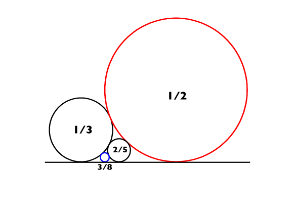
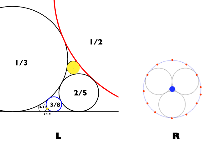
Figure 6: Upper Figure shows the Ford circle representation of the center ($3/8$ blue) and the left ($1/3$ black) and the right ( $2/5$ black). These three circles along with the horizontal black line are mutually tangent . We note that the scaling ratio between the red and the blue circles, corresponding to two consecutive generations of the butterfly asymptotically equals the ratio of the curvatures of the innermost ( solid blue) and the outermost circles ( with red dots) of the Apollonian gaskets with near $D_{3}$ symmetry ( Lower right). Lower left is the blowup of the upper figure with additional level of the hierarchy. The yellow circles ( big and small) are respectively the image of the horizontal axis reflected through the tangency points of the circles corresponding to $1/3,2/5,1/2$ and $4/11,7/19,3/8$. We note that these two consecutive image circles also scale by the same ratio $(\zeta^{*})^{2}$.

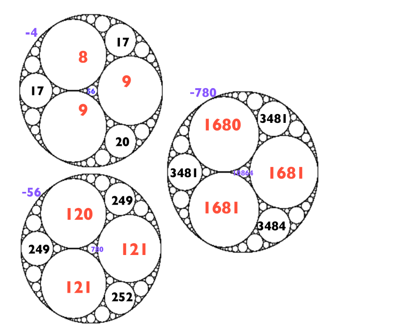
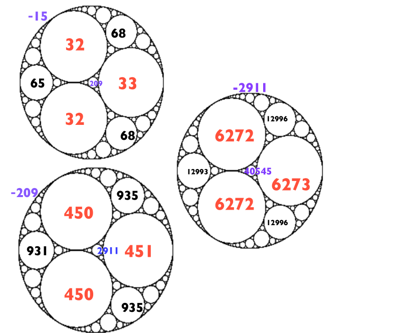
Figure 7: Circles show sequential construction of Apollonian gaskets where the upper (lower) three circles show three generations beginning with $(-4,8,9,9)$ ( $(-15,32,32,33)$ ) corresponding to even-$n$ ( odd-$n$) case. Note that the bounding circles with negative curvatures encode the chern numbers shown in the first row of Table I. Asymptotically, the Apollonian gasket exhibits $D_{3}$ symmetry. Also, note that all equivalent circles, asymptotically, scale by the same factor $\zeta^{2}$ as shown by converging ratios in the figure and hence show the flux scaling intervals of the butterflies.

The topological and magnetic flux scaling of the butterfly fractal is related to Apollonian gaskets. The Appendix provides a brief introduction to these fractals and discusses its properties that are key to understand the relationship between the butterfly fractal and the Apollonian gaskets.

The central concept that links Apollonian gaskets and the butterfly is hidden in the pictorial representations of fractions using Ford circles. We now discuss this relationship. Brief introduction to Ford circles is given in the Appendix.

V.1 Ford Circles, Apollonian Gasket and the Butterfly

As stated in the Appendix, a fraction $f=\frac{p}{q}$ can be represented by a circle ( Ford circle ) , with curvature ( inverse radius) $\kappa=2q^{2}$. These Ford circles also provide a pictorial representation of the size of the magnetic flux intervals. Using the Eq. (7),

$$\sqrt{\kappa_{c}(l+1)}=4\sqrt{\kappa_{c}(l)}-\sqrt{\kappa_{c}(l-1)}$$ (34)

The Ford circles do not touch and are all tangent to the horizontal axis of the butterfly graph. Introducing a scale factor $\zeta(l)$ as,

$$\zeta(l)=\sqrt{\frac{\kappa_{c}(l+1)}{\kappa_{c}(l)}},$$ (35)

we obtain,

$$\zeta(l)=4-\frac{1}{\zeta(l-1)}$$ (36)

For large $l$, $\zeta(l)\rightarrow\zeta(l+1)$, which we denote as $\zeta^{*}$, which satisfies the quadratic equation,

$$(\zeta^{*})^{2}-4\zeta^{*}+1=0,\quad\zeta^{*}=\lim_{l\rightarrow\infty}\sqrt{\frac{\kappa_{c}(l+1)}{\kappa_{c}(l)}}=2+\sqrt{3}$$ (37)

Therefore, Ford circles corresponding to even-denominator fractions form a self-similar fractal consisting of circles whose curvatures scale asymptotically by $\zeta^{*}$. Interestingly, starting with different even-denominator fraction, we get a different set, all exhibiting the same scaling. We note that,

$$\sqrt{\frac{\kappa_{c}(l)}{\kappa_{L}(l)}}\rightarrow 1+\sqrt{3},\quad\sqrt{\frac{\kappa_{c}(l)}{\kappa_{R}(l)}}\rightarrow\frac{1+\sqrt{3}}{\sqrt{3}},\quad\sqrt{\frac{\kappa_{R}(l)}{\kappa_{L}(l)}}\rightarrow\sqrt{3}$$ (38)

Figure (6) shows the Ford circle representation of the levels $0$ and $1$ of the butterfly centers $f_{c}$ and the boundaries, $f_{L},f_{R}$. In general, any two successive levels $l$ and $l+1$ of the butterfly flux intervals, we have two configurations which we list below, of four mutually tangent circles with curvatures $k_{i},i=1-4$ representing fractions

(1) $f_{c}(l),f_{L}(l+1),f_{R}(l+1)$ and base line are mutually tangent where $k_{1}\equiv k_{c}(l)=2q_{c}^{2}(l)$, $k_{2}\equiv k_{L}(l+1)=2q_{L}^{2}(l+1)$, $k_{3}\equiv k_{R}(l+1)=2q_{R}(l+1)^{2}$ and the base line with $k_{4}=0$ and

(2) $f_{c}(l+1),f_{L}(l+1),f_{R}(l+1)$ are mutually tangent where $k_{1}\equiv k_{c}(l)=2q_{c}^{2}(l)$, $k_{2}\equiv k_{L}(l+1)=2q_{L}^{2}(l+1)$, $k_{3}\equiv k_{R}(l+1)=2q_{R}(l+1)^{2}$ and the base line with $k_{4}=0$

From Descartes’s theorem ( Eq. (46)), we obtain

$$k_{c}(\pm)=k_{R}(l+1)\pm k_{L}(l+1),$$ (39)

where we can identify,

$$k_{c}(+)=k_{c}(l+1),\quad k_{c}(-)=k_{c}(l)$$ (40)

These two configurations describing butterfly fractal at two successive generations are in fact mirror image of each other, through a circle drawn from the tangency point of $f_{L}(l+1)$, $f_{R}(l+1)$ and the base line. In other words, the circles with curvatures $k_{c}(l)$ and $k_{c}(l+1)$ play the same role as the outermost and innermost circles of the Apollonian gasket in the configuration described on the right in Fig (6).

To see explicitly how the scaling ratio for the inner and the outermost radius of the Apollonian gasket is identical to that of the scaling ratio between the flux -intervals for two successive generations of the butterfly, we note that from Eq. (49), the ratio of the outer bounding circle and the innermost circles ( See Figs. (7) ) as obtained from Eq. (49) ) is,

$$\frac{k_{5}}{k_{4}}=\frac{2+\sqrt{3}}{2-\sqrt{3}}=7-4\sqrt{3}=\zeta^{2}$$ (41)

Therefore, the ratio of the bounding to the inner-most circle describe the scaling of the magnetic flux intervals of the butterfly. See Fig. (7).

$$\frac{k_{4}(+)}{k_{4}(-)}=\frac{2+\sqrt{3}}{2-\sqrt{3}}$$ (42)

In the case of butterfly, we have,

$$\sqrt{k_{c}(\pm)}=\sqrt{k_{R}(l+1)}\pm\sqrt{k_{L}(l+1)}=(\sqrt{3}\pm 1)\sqrt{k_{L}(l+1)},$$ (43)

which gives,

$$\frac{k_{c}(+)}{k_{c}(-)}=\frac{k_{c}(l+1)}{k_{c}(l)}=\frac{2+\sqrt{3}}{2-\sqrt{3}}$$ (44)

As described above, configuration of circles underlying the butterfly fractal appears to be a special case of a general construction involving four mutually tangent circles. However, we note that if we consider the mirror image of the horizontal (base) line through the tangency points of the Ford circles corresponding to $f_{L}(l+1),f_{R}(l+1),f_{c}(l)$ and $f_{L}(l+1),f_{R}(l+1),f_{c}(l+1)$ ( See Fig. (6)) , we obtain configuration involving four mutually tangent circles, each corresponds to non-zero curvature. This puts butterfly fractal closer to the Apollonian gasket. We finally remark that although the image circles of the horizontal line do not correspond to butterflies symmetric about $E=0$, their size scale by the same ratio $\zeta$ and may correspond to off-centered patterns that are beyond the subject of this paper.

Figure (7) shows the integral Apollonian gaskets, exhibiting hierarchical set of integers that describe quantum numbers of the butterfly obtained by zooming the interval $[1/3-2/5]$. To obtain complete hierarchy, of topological integers, we begin with two sets of Apollonian gaskets with curvatures $(2,2,3,-1)$ and $(8,9,9,-4)$, and use the recursion relation (7) for the negative curvatures. We obtain all the Chern numbers as listed in the first row of Table I , in fact all equivalent circles scale by $\zeta^{2}$ suggests that the butterfly fractal characterized by the Farey path ”LRL” corresponding to the whole set of irrationals $\zeta_{12}$ are described by the Apollonian gasket.

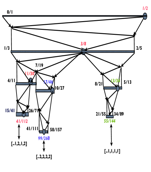
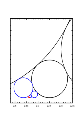
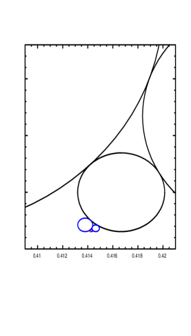
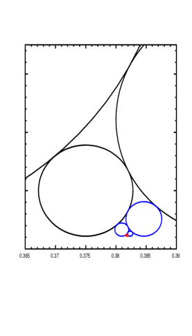
Figure 8: Upper graph is a schematically representation of magnetic flux intervals of the butterfly fractal for three levels of nesting showing $\zeta_{12}$ , $\zeta_{2}$ and $\zeta_{1}$ hierarchies, all starting with the common level-$1$ sub-interval $1/3-2/5$. Lower graph shows the corresponding Fords circles ( from left-right ) for $\zeta_{1,2}$, $\zeta_{2}$ and $\zeta_{1}$ hierarchies for level-$1$ ( black), level-$2$ (blue) and level-$3$ (red). This pictorial representation of the center and the boundaries of the butterfly illustrate distinctions between the these three hierarchies where the golden-tail butterfly flips between two successive levels. The entire butterfly plot obtained numerically in shown in Fig. (9).

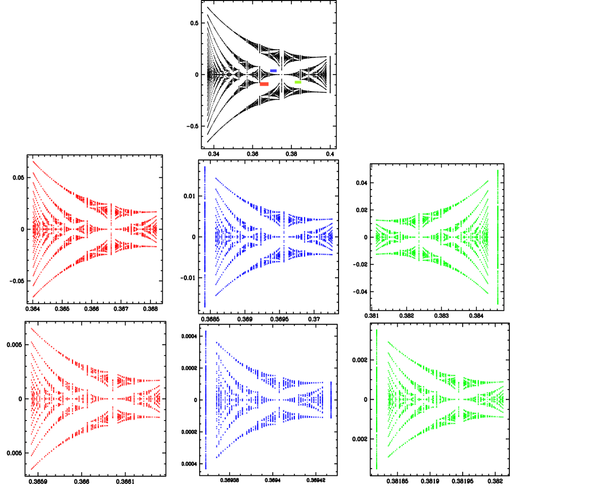
Figure 9: Butterfly plots for three levels for $\zeta_{12}$ ( red), $\zeta_{2}$ ( blue ) and $\zeta_{1}$ (green) hierarchies, all starting from the black butterfly at the top. The horizontal lines on the black plot show the appropriate window that is zoomed and displayed below. We note that golden-mean hierarchy has its butterfly flips between two successive generations.

$\phi^{*}_{c}$	Recursion relations for $q_{x},p_{x}\equiv s$	$R_{\phi}$	$\approx$ $R_{E}$	Farey path
$\zeta_{1,2}$= $[...1,2,1,2....]$	$s(l+1)=4s(l)-s(l-1)$	$2+\sqrt{3}=3.73205$	10	LRL
$\zeta_{1}$= $[...1,1,1,1....]$	$s(l+1)=4s(l)+s(l-1)$	$2+\sqrt{5}=4.236068$	14	LRLRLR
$\zeta_{2}$= $[...2,2,2,2...]$	$s(l+1)=6s(l)-s(l-1)$	$2\sqrt{2}+3=5.82843$	38	LRRL

Table 3: Comparing the scaling ratios $R_{\phi}$ and $R_{E}$ for various irrational fluxes whose even denominator approximants form the fixed points of the centers of the butterfly. Each irrational value describes a set of numbers with same tail in the continued fraction expansion.

VI Golden and Silver Mean Hierarchies

As discussed above, we have investigated the entire Gplot by zooming in the equivalent sets of butterflies and calculating the asymptotic scaling properties of the fixed point butterfly fractal. In contrast, earlier studies have explored the butterfly fractal by starting with a fixed irrational number. We briefly investigate this line of analysis of the butterfly fractal for the golden and the silver mean flux values. We follow the irrational magnetic flux by following a sequence of its rational approximants with even denominators where the relation between the boundaries and the center is always given by, $f_{c}(l)=f_{L}(l)\bigoplus f_{R}(l)$. However, the ordered set of three rationals $f_{L}$, $f_{c}$ and $f_{R}$ , need not belong to the set of rational approximants of the irrational magnetic flux.

For the golden-mean $\gamma_{g}=(\sqrt{5}-1)/2$ , its even denominator approximants $(1/2,3/8,13/34,55/144,233/610...)$ form the centers of the butterfly at $E=0$ with Chern numbers $(1,4,17,72,305....)$. As shown in upper part of the Fig. (8), the centers do not form a monotonic sequence and therefore the equivalent set of butterflies correspond to the Farey path $LRLRLR$ or $RLRLRL$.

The silver-mean $\gamma_{s}=\sqrt{2}-1$ with rational approximants ($1/2,2/5,5/12,12/29,29/70,70/169,169/408....$) result in an silver hierarchy with Chern numbers $(1,6,35,204...)$ and correspond to the Farey path $LRRL$ .

Table III compares the three hierarchies which we will also refer as diamond, silver and golden hierarchy. Figure (9) shows the three generations of the butterflies and clearly illustrate the dominance of diamond hierarchy as the scale factors for both the $\phi$ and the $E$ intervals are smaller than the corresponding scale factors for the silver and golden cases.

We also note that unlike diamond hierarchy, silver and golden mean hierarchies do not map to integral Apollonian gaskets.

As a final comparison between three irrationals, we look at the three Polygons, as shown in Fig. (11) whose angles relate to these irrationals. Mathematical simplicity of the diamond mean is rather intriguing and it remains to be seen if the area of dodecagonal being equal to $2R^{2}$ ( where $R$ is the radius of the circle ) provides any further insight towards its relationship to $D_{3}$ symmetry of the Apollonian gasket.

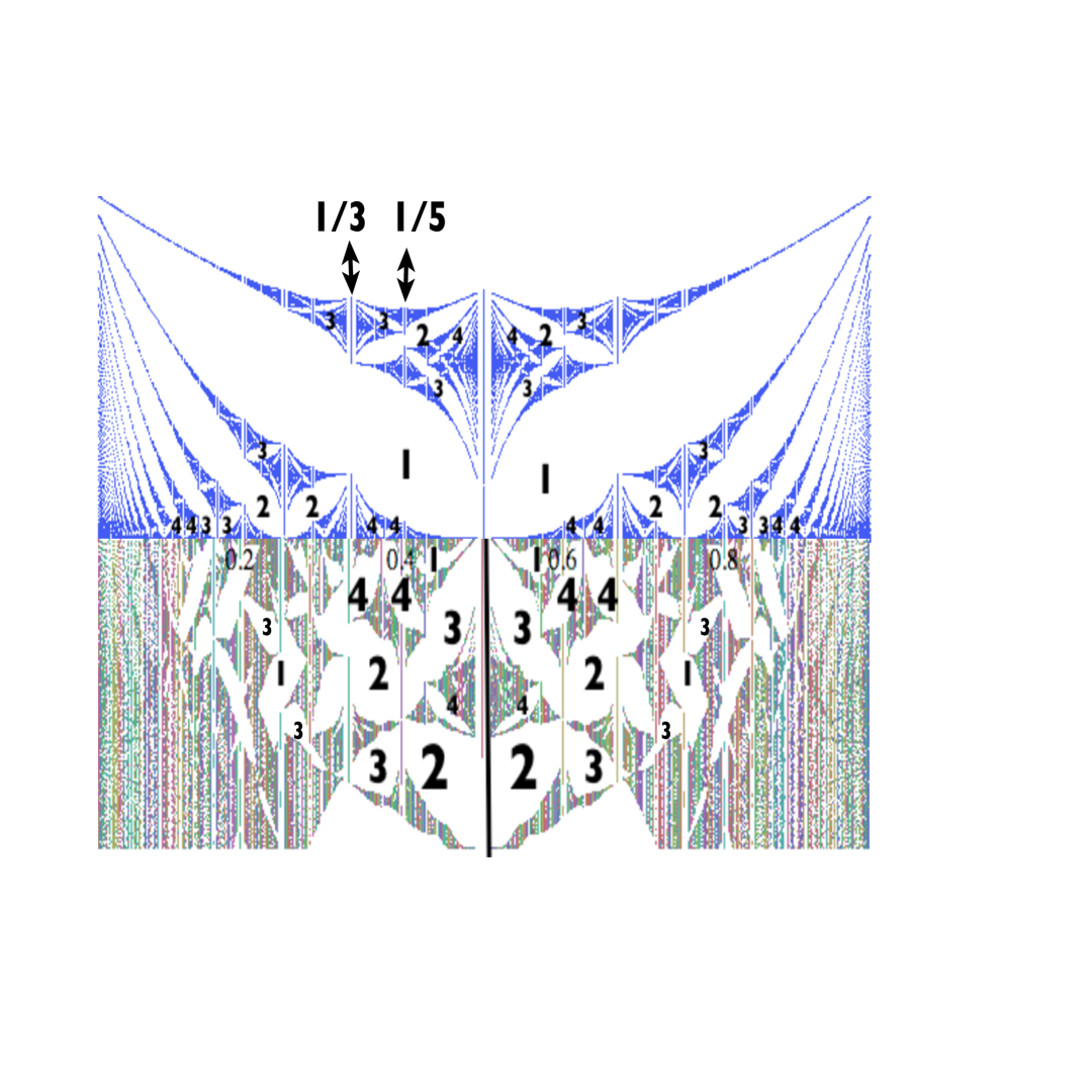
Figure 10: (color on line) Upper half of the butterfly spectrum for static ($J_{x}=J_{y}$)(upper) and lower-half of the quasienergy spectrum for driven system with $\bar{J}=.33,\bar{\lambda}=1.1$ (lower). Dominance of higher Chern states in kicked system is due to phase transitions where Chern-$1$ state for $\phi=1/3$ is transformed into Chern $-2(=1-3)$ state while Chern ($-2$, $1$) states of $\phi=2/5$ evolve into Chern $3(=-2+5)$,$-4(=1-5)$ states.

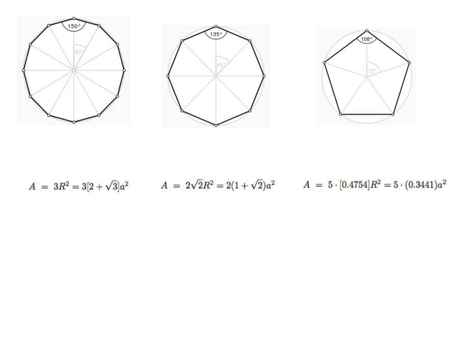
Figure 11: Polygons whose angles relate to the three irrational numbers. Here $R$ is the radius of the circumscribed circle, $a$ is the length of the side of the regular polygon and $A$ is the area of the polygon. From left to right , the polygons with vortex angles $30,45,72$ degrees or equivalently $\frac{2\pi}{12}$, $\frac{2\pi}{8}$ and $\frac{2\pi}{5}$ radian reveal relationship between the three irrationals and the corresponding $12,8,5$ fold symmetry. The area A reveals hidden mathematical simplicity of the diamond mean.

VII Periodic Driving and Gap Amplification

We next address the question of physical relevance of states of higher topological numbers in view of the fact that size of the spectral gaps decreases exponentially with $\sigma$, as confirmed by our numerical study of the system described by Eq. (3). We now show that by perturbing such systems, we can induce quantum phase transitions to topological states with $n>0$ given by (4) with dominant gaps characterized by higher Chern numbers. We study butterfly spectrum for a periodically kicked quantum Hall systemLababidi et al. (2014) where $J_{y}$ is a periodic function of time $t$ with period-$T$Lababidi et al. (2014),

$$J_{y}=\lambda\sum_{n}\delta(t/T-n)$$ (45)

The time evolution operator of the system, defined by $|\psi(t)\rangle=U(t)|\psi(0)\rangle$, has the formal solution $U(t)={\cal T}\exp[-i\int^{t}_{0}H(t^{\prime})dt^{\prime}]$, where ${\cal T}$ denotes time-ordering and we set $\hbar=1$ throughout. The discrete translation symmetry $H(t)=H(t+T)$ leads to a convenient basis $\{|\phi_{\ell}\rangle\}$, defined as the eigenmodes of Floquet operator $U(T)$,

$$U(T)|\phi_{\ell}\rangle=e^{-i\omega_{\ell}T}|\phi_{\ell}\rangle.$$

We have two independent driving parameters, $\bar{J}=J_{x}T/\hbar$ and $\bar{\lambda}=\lambda T/\hbar$. For rational flux $\phi=p/q$, $U$ is a $q\times q$ matrix with $q$ quasienergy bands that reduce to the energy bands of the static system as $T\rightarrow 0$.

New topological landscape of the driven system as shown in the Fig. (10) can be understood by determining the topological states of flux values corresponding to simple rationals such as $1/3$, $2/5$. In the Fig. (10), parameter values correspond to the case where the Chern-$1$ gap associated with $1/3$ has undergone quantum phase transition to a $n=1$ solution of the DE (Eq. (4)) and the Chern-$-2,1$ states of $2/5$ have also undergone transitions to Chern-$3,-4$ state. This almost wipes out the Chern-$1$ state from the landscape, exposing the topological states of higher Cherns that existed in tiny gaps in the static system. We note that, topological invariants associated with irrational flux values can not change under driving and in view of infinite set of irrationals in the vicinity of every rational, the ordering of the Cherns as we vary the filling factor remains unchanged.

Gap amplifications of states in periodically driven quantum hall system may provide a possible pathway to see fractal aspects of Hofstadter butterfly and engineer states with large Chern numbers experimentally. Recent experiments with ultracold atomsLin et al. (2009) Zhao et al. (2011) and shaken optical latticesZheng and Zhai (2014) offer a promising means to realize the butterfly and its transformation in driven systems.

VIII Conclusions and Open Questions

The unveiling of a dodecagonal quasicrystalMacDonald (1989), also characterized by integral Apollonian gasket with $D_{3}$ symmetry that fully encodes the topological hierarchy of the butterfly fractal is the central result of this paper. However, the relationship between these two symmetries remain obscure. We note that these results also apply to other 2D lattices such as graphene in the magnetic field. The associated scaling for topological quantum numbers is universal, independent of lattice symmetry and perhaps indicates result of greater validity and significance. Why dodecagonal quasicrystals emerge as the dominant hierarchy remains an open question. The fact that only these symmetries map to integral Apollonian gaskets makes the puzzle deeper and more intriguing. Emergence of hidden symmetries, as energy scale approaches zero is reminiscent of phenomena such as asymptotic freedom in Quantum Chromodynamics.

Recently, there is renewed interest in quasiperiodic systemsKraus and Zilberberg (2012); Satija and Naumis (2013); Dana (2014) due to their exotic characteristics that includes their relationship to topological insulators. Our findings about new symmetries and topological universality will open new avenues in the study of interplay between topology and self-similarity in frustrated systems.

Appendix A Geometrical Representation of Fractions: Farey Tree, Ford Circles and Descartes’ Theorem

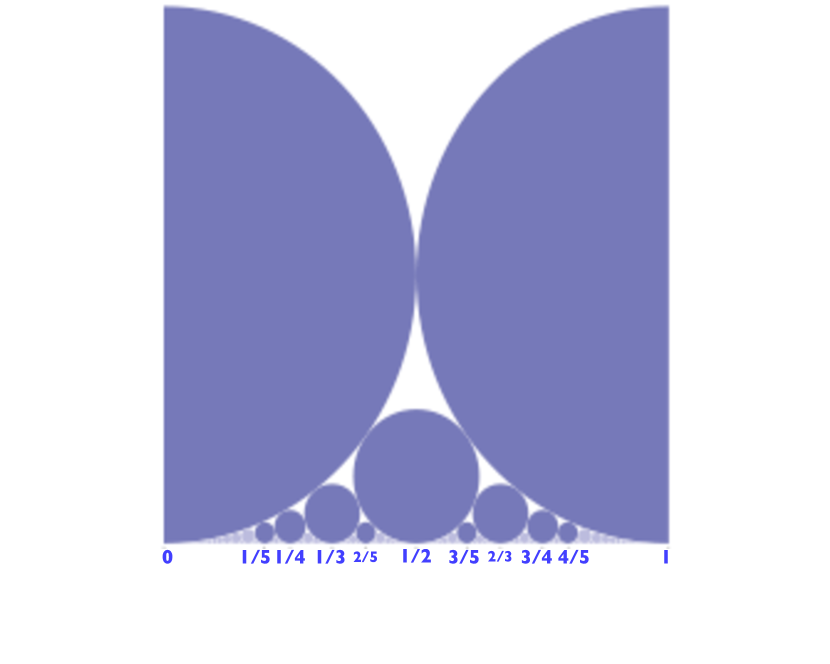
Figure 12: Ford circles provide geometrical representation of Farey sequences. Figure where every fraction $p/q$ is associated with a circle of radius $\frac{1}{2q^{2}}$, describes a special case of Descartes’s theorem as the straight line is a circle of zero curvature.

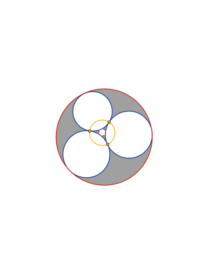
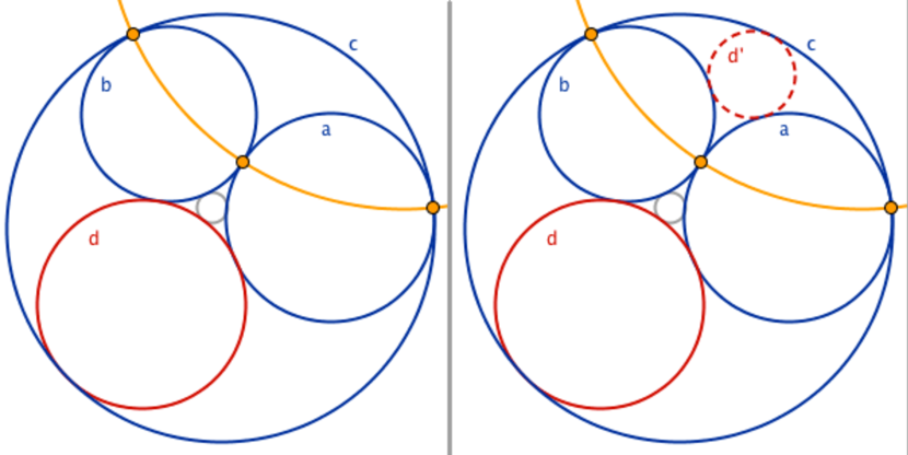
Figure 13: Upper graph illustrates reflection through a circle in a configuration involving four mutually tangent circles. Smallest ( dashed red) and largest ( red) circles are mirror image of each other through reflection through the yellow circle, a circle drawn through the tangency points of the three circle. The lower graphs illustrates this further, highlighting the preservation of tangency. The red circle (d) tangent to the three blue circles, $a,b,c$, and its reflection in the yellow circle, drawn at the tangency points of the circles $a,b,c$, producing the image ( dotted red) circle labeled $d^{\prime}$. Create a circle through the intersection points of three mutually tangent circles. The three tangent circles are blue in the picture below.

Farey Sequences of order $n$ is the sequence of completely reduced fractions between $0$ and $1$, which have denominators less than or equal to n, arranged in order of increasing size. We note that two neighboring terms say $\frac{p1}{q1}$ and $\frac{p2}{q2}$ in any Farey sequence satisfy the equation $|q1p2-q2p1|=1$ and their difference $|\frac{p1}{q1}-\frac{p2}{q2}|=\frac{1}{q1q2}$. Of all fractions that are neighbors of $\frac{p}{q}$ ( $q>1$ ) only two have denominators less than $q$. It is this property that associates a unique pair $p_{L}/q_{L}$ and $p_{R}/q_{R}$ with a fraction $p_{c}/q_{c}$ when $q_{c}$ is even and $q_{L}<q_{c}$ and $q_{R}<q_{c}$ are oddFord (1938).

Ford Circles ( See Fig. (12)) provide geometrical representation of fractionsFord (1938). For every fraction $\frac{p}{q}$ (where $p$ and $q$ are relatively prime) there is a Ford circle, which is the circle with radius $\frac{1}{2q^{2}}$ and center at $\frac{p}{q}$ and tangent to the base line. Two Ford circles for different fractions are either disjoint or they are tangent to one another. In other words, two Ford circles never intersect. If $0<\frac{p}{q}<1$, then the Ford circles that are tangent to the ford circle centered at $\frac{p}{q}$, are precisely the Ford circles for fractions that are neighbors of $\frac{p}{q}$ in some Farey sequence.

Three mutually tangent Ford circles in the Fig. (12), along with the base line that can be thought of as a circle with infinite radius, are a special case of four mutually tangent circles such as those shown in Fig. (6 R). Relation between the radii of four such mutually tangent circles is given by Descartes’s theorem.

Descartes’s theorem states that if four circles are tangent to each other, and the circles have curvatures ( inverse of the radius) $k_{i}$ (for $i=1,...,4$), a relation between the curvatures $k_{i}$ of these circles is given by,

$$(k_{1}+k_{2}+k_{3}+k_{4})^{2}=2(k_{1}^{2}+k_{2}^{2}+k_{3}^{2}+k_{4}^{2}).$$ (46)

Solving for $k_{4}$ in terms of $k_{i}$, $i=1,2,3$ gives,

$$k_{4}=k_{1}+k_{2}+k_{3}\pm 2\sqrt{k_{1}k_{2}+k_{2}k_{3}+k_{3}k_{1}}$$ (47)

The two solutions $\pm$ respectively correspond to the inner ( solid blue circle) in Fig. (6 R ) and the outer bounding circle ( circle with red dots ). The consistent solutions of above set of equations require that bounding circle must have negative curvature. Denoting the curvature of the inner circle as $k_{5}$, it follows that

$$k_{4}+k_{5}=2(k_{1}+k_{2}+k_{3})$$ (48)

Important consequence of the Eq. (48) is the fact that if $k_{i},i=1-4$ are integers, $k_{5}$ is also an integer.

Patterns obtained by starting with three mutually tangent circles and then recursively inscribing new circles in the curvilinear triangular regions formed between the circles are Known as the Apollonian gasket, or Curvilinear Sierpinski Gasket, as the three mutually tangent circles form a triangle in curved space. An Apollonian gasket describes a packing of circles arising by repeatedly filling the interstices between four mutually tangent circles with further tangent circles.

Integral Apollonian Gasket has all circles whose curvatures are integers. As described above, such a fractal made up integers alone can be constructed if the first four circles have integer curvatures. ( See figs (7)).

Apollonian gaskets with $D_{3}$ symmetry is a fractal with $D_{3}$ symmetry, which corresponds to three reflections along diameters of the bounding circle (spaced $120$ degrees apart), along with three-fold rotational symmetry. Such a gasket can be constructed if the three circles with smallest positive curvature have the same curvature. Setting $k_{1}=k_{2}=k_{3}=k$ in Eq. (47), we obtain

$$k_{4}({\pm})=(3\pm 2\sqrt{3})k$$ (49)

The fact that the ratio $k_{4}/k$ is an irrational number means that no integral Apollonian circle packing possesses $D_{3}$ symmetry, although many packings come close. As illustrated in the Fig. (7), this symmetry is restored in the iterative process where the inner circle at level $l$ becomes the outer circle at level $l+1$.

Apollonian Gasket-Kaleidoscope Another remarkable property of the Apollonian gasket is that the whole Apollonian gasket is like a kaleidoscope where the image of the first four circles is reflected again and again through an infinite collection of curved mirrors.

This is illustrated in Fig. (13) using an operation called inversion, a classic tool to understand configurations involving mutually tangent circles, which is can be thought of as a reflection through a circle. The key feature of the inversion that maps circles to circles, is that it preserves tangency as both the circle and its reflected image are tangent to same set of circles as illustrated in Fig. (13).

References

- Hofstadter (1976) D. R. Hofstadter, Physical Review B 14, 2239 (1976).
- Hopstadter (1989) D. Hopstadter, The world ”Gplot” was used by Hofstadter after a friend of his struck by infinitely many infinities of the plot called it a picture of Go: Godel Escher and Bach (Vintage Books Edition, 1989).
- Thouless et al. (1982) D. J. Thouless, M. Kohmoto, M. P. Nightingale, and M. den Nijs, Physical Review Letters 49, 405 (1982).
- Dean et al. (2013) C. R. Dean, L. Wang, C. Maher, Forsythe, Ghahari, F. Gao, J. Katoch, M. shigami, P. Moon, M. Koshino, T. Taniguchi, K. Watanabe, K. L. Shepard, H. J, and P. Kim, Nature 45, 12186 (2013).
- Aidelsburger et al. (2013) M. Aidelsburger, M. Atala, M. Lohse, J. T. Barreiro, B. Paredes, , and I. Bloch, Physical Review Letter 111, 108301 (2013).
- Weld et al. (2013) D. Weld, P. Medley, H. Miyake, D. Hucul, D. Pritchard, and W. Ketterle, Physical Review Letters 111, 108302 (2013).
- Wannier (1978) G. H. Wannier, Phys Status Solidi B 88, 757 (1978).
- MacDonald (1983) A. MacDonald, Physical Review B 88, 6713 (1983).
- Wilkinson (1987) M. Wilkinson, Journal of Physics A, Math. Gen. 20, 4337 (1987).
- Wilkinson (1994) M. Wilkinson, Journal of Physics A, Math. Gen. 21, 8123 (1994).
- Chang and Niu (1996) M.-C. Chang and Q. Niu, Physical Review B 53, 7010 (1996).
- MacDonald (2009) A. MacDonald, Journal of Physics, B 42, 055302 (2009).
- Dana I (1985) Z. J. Dana I, Avron Y, Journal of Physics, C, Solid State 18, L679 (1985).
- Hardy and Wright (1979) Hardy and Wright, Introduction to theory of Numbers, 1st ed. (Oxford University Press, 1979).
- MacDonald (1989) A. MacDonald, Physical Review B 39, 10519 (1989).
- Mandelbrot (1982) B. Mandelbrot, Fractal Geometry of Nature (Cambridge University Press, 1982).
- Lin et al. (2009) Y.-J. Lin, R. L. Compton, K. Jiménez-García, J. V. Porto, and I. B. Spielman, Nature 462, 628 (2009).
- Harper (1955) P. G. Harper, Proc of Physical Society of London A68, 874 (1955).
- Lababidi et al. (2014) M. Lababidi, I. I. Satija, and E. Zhao, Physical Review Letters 112, 026805 (2014).
- Zhao et al. (2011) E. Zhao, N. Bray-Ali, C. J. Williams, I. B. Spielman, and I. I. Satija, Phys. Rev. A 84, 063629 (2011).
- Zheng and Zhai (2014) W. Zheng and H. Zhai, arXiv:1402.4034 [cond-mat] (2014), arXiv: 1402.4034.
- Kraus and Zilberberg (2012) Y. E. Kraus and O. Zilberberg, Physical Review Letters 109, 116404 (2012).
- Satija and Naumis (2013) I. I. Satija and G. Naumis, Physical Review B 88, 054204 (2013).
- Dana (2014) I. Dana, Phys. Rev. B 89, 205111 (2014).
- Ford (1938) L. R. Ford, The American Mathematical Monthly 39, 586 (1938).