Generalizing Block LU Factorization:
A Lower-Upper-Lower Block Triangular Decomposition with Minimal Off-Diagonal Ranks

Abstract

We propose a novel factorization of a non-singular matrix $P$, viewed as a $2\times 2$-blocked matrix. The factorization decomposes $P$ into a product of three matrices that are lower block-unitriangular, upper block-triangular, and lower block-unitriangular, respectively. Our goal is to make this factorization “as block-diagonal as possible” by minimizing the ranks of the off-diagonal blocks. We give lower bounds on these ranks and show that they are sharp by providing an algorithm that computes an optimal solution. The proposed decomposition can be viewed as a generalization of the well-known Block LU factorization using the Schur complement. Finally, we briefly explain one application of this factorization: the design of optimal circuits for a certain class of streaming permutations.

1 Introduction

Given is a non-singular matrix $P\in GL_{m+n}(\mathbb{K})$ over a field $\mathbb{K}$. We partition $P$ as

$$P=\begin{pmatrix}P_{1}&P_{2}\\ P_{3}&P_{4}\\ \end{pmatrix},\quad\text{such that $P_{1}$ is $m\times m$}.$$

We denote the ranks of the submatrices with $p_{i}=\operatorname{rk}P_{i}$, $i=1,2,3,4$. Matrices are denoted with capital letters and vector spaces with calligraphic letters.

If $P_{1}$ is non-singular, then a block Gaussian elimination uniquely decomposes $P$ into the form:

$$P=\begin{pmatrix}I_{m}&\\ L&I_{n}\\ \end{pmatrix}\begin{pmatrix}C_{1}&C_{2}\\ &C_{4}\\ \end{pmatrix},$$ (1)

where $I_{m}$ denotes the $m\times m$ identity matrix. The rank of $L=P_{3}P_{1}^{-1}$ is equal to $p_{3}$, and $C_{4}$ is the Schur complement of $P_{1}$. Conversely, if such a decomposition exists for $P$, then $P_{1}$ is non-singular. This block LU decomposition has several applications including computing the inverse of $P$ [2], solving linear systems [4], and in the theory of displacement structure [6]. The Schur complement is also used in statistics, probability and numerical analysis [11, 3].

Analogously, the following decomposition exists if and only if $P_{4}$ is non-singular:

$$P=\begin{pmatrix}C_{1}&C_{2}\\ &C_{4}\\ \end{pmatrix}\begin{pmatrix}I_{m}&\\ R&I_{n}\\ \end{pmatrix}.$$ (2)

This decomposition is again unique, and the rank of $R$ is $p_{3}$.

In this article, we release the restrictions on $P_{4}$ and $P_{1}$ and propose the following decomposition for a general $P\in GL_{m+n}(\mathbb{K})$:

$$P=\begin{pmatrix}I_{m}&\\ L&I_{n}\\ \end{pmatrix}\begin{pmatrix}C_{1}&C_{2}\\ &C_{4}\\ \end{pmatrix}\begin{pmatrix}I_{m}&\\ R&I_{n}\\ \end{pmatrix},$$ (3)

where in addition we want the three factors to be “as block-diagonal as possible,” i.e., that $\operatorname{rk}L+\operatorname{rk}C_{2}+\operatorname{rk}R$ is minimal.

1.1 Lower bounds

The following theorem provides bounds on the ranks of such a decomposition:

Theorem 1.

If a decomposition (3) exists for $P\in GL_{m+n}(\mathbb{K})$, it satisfies

$$\operatorname{rk}C_{2}=p_{2},$$ (4)

$$\operatorname{rk}L\geq n-p_{4},$$ (5)

$$\operatorname{rk}R\geq m-p_{1},$$ (6)

$$\operatorname{rk}R+\operatorname{rk}L\geq p_{3}.$$ (7)

In particular, the rank of $C_{2}$ is fixed and we have:

$$\operatorname{rk}R+\operatorname{rk}L\geq\max(p_{3},n+m-p_{4}-p_{1}).$$ (8)

We will prove this theorem in Section 4. Next, we assert that these bounds are sharp.

1.2 Optimal solution

The following theorem shows that the inequality (8) is sharp:

Theorem 2.

If $P\in GL_{m+n}(\mathbb{K})$, then there exists a decomposition (3) that satisfies

$$\begin{array}[]{cc}\operatorname{rk}R+\operatorname{rk}L=\max(p_{3},n+m-p_{4}-p_{1})\text{ and}\\ \operatorname{rk}L=n-p_{4}.\end{array}$$

Additionally, such a decomposition can be computed with $O((m+n)^{3})$ arithmetic operations.

We prove this theorem in Section 5 when $p_{3}\leq m+n-p_{4}-p_{1}$, and in Section 6 for the case $p_{3}>m+n-p_{4}-p_{1}$. In both cases, the proof is constructive and we provide a corresponding algorithm (Algorithms 3 and 4). Theorem 2 and the corresponding algorithms are the main contributions of this article.

Two cases. As illustrated in Figure 1, two different cases appear from inequality (8). If $p_{3}\leq m+n-p_{4}-p_{1}$, bound (7) is not restrictive, and the optimal pair $(\operatorname{rk}L,\operatorname{rk}R)$ is unique, and equals $(n-p_{4},m-p_{1})$. In the other case, where $p_{3}>m+n-p_{4}-p_{1}$, bound (7) becomes restrictive, and several optimal pairs $(\operatorname{rk}L,\operatorname{rk}R)$ exist.

Figure 1: Possible ranks for $L$ and $R$. On the left graph, $p_{3}<m+n-p_{4}-p_{1}$. On the right graph, $p_{3}>m+n-p_{4}-p_{1}$. The dot shows the decomposition provided by Theorem 2.

Example. As a simple example we consider the special case

$$P=\begin{pmatrix}&P_{2}\\ P_{3}&\end{pmatrix},\quad\text{with }n=m.$$

In this case $P_{3},\ P_{2}$ are non-singular and neither (1) nor (2) exists. Theorem 1 gives a lower bound of $\operatorname{rk}R+\operatorname{rk}L\geq 2n$, which implies that both $R$ and $L$ have full rank. Straightforward computation shows that for any non-singular $L$,

$$P=\begin{pmatrix}I_{n}&\\ L&I_{n}\end{pmatrix}\begin{pmatrix}L^{-1}P_{3}&P_{2}\\ &-LP_{2}\end{pmatrix}\begin{pmatrix}I_{n}&\\ -(LP_{2})^{-1}P_{3}&I_{n}\end{pmatrix}$$

is an optimal solution. This also shows that the optimal decomposition (3) is in general not unique.

1.3 Flexibility

The following theorem adds flexibility to Theorem 2 and shows that a decomposition exists for any Pareto-optimal pair of non-diagonal ranks that satisfies the bounds of Theorem 1:

Theorem 3.

If $P\in GL_{m+n}(\mathbb{K})$ and $(l,r)\in\mathbb{N}^{2}$ satisfies $l\geq n-p_{4},\ r\geq m-p_{1}$, and

$$r+l=\max(p_{3},n+m-p_{4}-p_{1}),$$

then $P$ has a decomposition (3) with $\operatorname{rk}L=l$ and $\operatorname{rk}R=r$.

In the case where $p_{3}\leq m+n-p_{4}-p_{1}$, the decomposition produced by Theorem 2 has already the unique optimal pair $(\operatorname{rk}L,\operatorname{rk}R)=(n-p_{4},m-p_{1})$. In the other case, we will provide a method in Section 7 to trade between the rank of $R$ and the rank of $L$, until bound (6) is reached. By iterating this method over the decomposition obtained in Theorem 2, decompositions with various rank tradeoffs can be built.

Therefore, it is possible to build decomposition (3) for any pair $(\operatorname{rk}L,\operatorname{rk}R)$ that is a Pareto optimum of the given set of bounds. As a consequence, if $f:\mathbb{N}^{2}\rightarrow\mathbb{R}$ is weakly increasing in both of its arguments, it is possible to find a decomposition that minimizes $f(\operatorname{rk}L,\operatorname{rk}R)$. Examples include $\min(\operatorname{rk}L,\operatorname{rk}R)$, $\max(\operatorname{rk}L,\operatorname{rk}R)$, $\operatorname{rk}L+\operatorname{rk}R$, $\operatorname{rk}L\cdot\operatorname{rk}R$ or $\sqrt{\operatorname{rk}^{2}L+\operatorname{rk}^{2}R}$.

Generalization of block LU factorization. In the case where $P_{4}$ is non-singular, Theorem 2 provides a decomposition that satisfies $\operatorname{rk}L=0$. In other words, it reduces to the decomposition (2). Using Theorem 3, we can obtain a similar result in the case where $P_{1}$ is non-singular. Since in this case $m-p_{1}=0$, it is possible to choose $r=0$, and thus obtain the decomposition (1).

1.4 Equivalent formulations

Lemma 1.

The following decomposition is equivalent to decomposition (3), with analogous constraints for the non-diagonal ranks:

$$P=\begin{pmatrix}I_{m}&\\ L_{3}&L_{4}\\ \end{pmatrix}\begin{pmatrix}C_{1}&C_{2}\\ &I_{n}\\ \end{pmatrix}\begin{pmatrix}I_{m}&\\ R_{3}&R_{4}\\ \end{pmatrix}$$ (9)

In this case, the minimization of the non-diagonal ranks is exactly the same problem as in (3). However, an additional degree of freedom appears: any non-singular $n\times n$ matrix can be chosen for either $L_{4}$ or $R_{4}$.

It is also possible to decompose $P$ into two matrices, one with a non-singular leading principal submatrix $L_{1}$ and the other one with a non-singular lower principal submatrix $R_{4}$:

$$P=\begin{pmatrix}L_{1}&L_{2}\\ L_{3}&L_{4}\\ \end{pmatrix}\begin{pmatrix}R_{1}&R_{2}\\ R_{3}&R_{4}\\ \end{pmatrix}$$ (10)

Once again, the minimization of $\operatorname{rk}L_{3}+\operatorname{rk}R_{3}$ is the same problem as in (3). The two other non-diagonal blocks satisfy $\operatorname{rk}L_{2}+\operatorname{rk}R_{2}\geq p_{2}$.

Proof.

The lower non-diagonal ranks are invariant through the following steps:

$\eqref{deco3}\Rightarrow\eqref{deco4}$. If $P$ has a decomposition (3), a straightforward computation shows that:

$$P=\begin{pmatrix}I_{m}&\\ L&C_{4}\\ \end{pmatrix}\begin{pmatrix}C_{1}&C_{2}\\ &I_{n}\\ \end{pmatrix}\begin{pmatrix}I_{m}&\\ R&I_{n}\\ \end{pmatrix},$$

which has the form of decomposition (9).

$\eqref{deco4}\Rightarrow\eqref{deco5}$. If $P$ has a decomposition (9), the multiplication of the two left factors leads to formulation (10). In fact, $L_{1}=C_{1}$ and $R_{4}$ are both non-singular.

$\eqref{deco5}\Rightarrow\eqref{deco3}$. If $P$ has a decomposition (10), then using (1) on the left factor, and (2) on the right factor, and multiplying the two central matrices leads to formulation (3). ∎

1.5 Related work

Schur complement. Several efforts have been made to adapt the definition of Schur complement in the case of general $P_{1}$ and $P_{4}$. For instance, it is possible to define an indexed Schur complement of another non-singular principal submatrix [11], or use pseudo-inverses [1] for matrix inversion algorithms.

Alternative block decompositions. A common way to handle the case where $P_{1}$ is singular is to use a permutation matrix $B$ that reorders the columns of $P$ such that the new principal upper submatrix is non-singular [11]. Decomposition (1) then becomes:

$$P=PBB^{T}=\begin{pmatrix}I_{m}&\\ L&I_{n}\\ \end{pmatrix}\begin{pmatrix}C_{1}&C_{2}\\ &C_{4}\\ \end{pmatrix}B^{T}$$

However, $B$ needs to swap columns with index $\geq m$; thus $B^{T}$ does not have the required form considered in our work.

One can modify the above idea to choose $B$ such that $B^{-1}$ has the shape required by decomposition (3):

$$P = \begin{pmatrix}P_{1}&P_{2}\\ P_{3}&P_{4}\end{pmatrix}\begin{pmatrix}I_{m}\\ -R&I_{n}\end{pmatrix}\begin{pmatrix}I_{m}\\ R&I_{n}\end{pmatrix}$$

$$= \begin{pmatrix}P_{1}-RP_{2}&P_{2}\\ P_{3}-RP_{4}&P_{4}\end{pmatrix}\begin{pmatrix}I_{m}\\ R&I_{n}\end{pmatrix}$$

Then the problem is to design $R$ such that $P_{1}-RP_{2}$ is non-singular and $\operatorname{rk}(P_{3}-RP_{4})+\operatorname{rk}R$ is minimal. This basic idea is used in [9], where, however, only $\operatorname{rk}R$ is minimized, which, in general, does not produce optimal solutions for the problem considered here.

Finally, our decomposition also shares patterns with a block Cholesky decomposition, or the Block LDL decomposition, in the sense that they involve block uni-triangular matrices. However, the requirements on $P$ and the expectations on the decomposition are different.

2 Application: Optimal Circuits for Streaming Permutations

The original motivation for considering our decomposition (3) was an important application in the domain of hardware design. Many algorithms in signal processing and communication consist of alternating computation and reordering (permutation) stages. Typical examples include fast Fourier transforms [10]; one example (a so-called Pease FFT) is shown in Fig. 2 for 16 data points. When mapped to hardware, permutations could become simple wires. However, usually, the data is not available in one cycle, but streamed in chunks over several cycles. Implementing such a “streaming” permutation in this scenario on an application-specific integrated circuit (ASIC) or on a field programmable gate array (FPGA) becomes complex, as it now requires both logic and memory [7, 9]. It turns out that for an important subclass of permutations called “linear,” the design of an optimal circuit (i.e., one with minimal logic) is equivalent to solving (3) in the field $\mathbb{F}_{2}$.

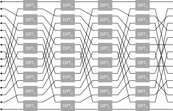
Figure 2: Dataflow of a Pease FFT on $16$ points from right (input) to left (output). Computing stages, consisting of DFTs on two points and pointwise multiplications (not shown), alternate with permutations.

Next, we provide a few more details on this application starting with the necessary background information. However, we only provide a sketch; a more complete treatment can be found in [9].

2.1 Linear permutations

For $0\leq i<2^{m+n}$, we denote with $i_{b}$ the associated (bit) vector in $\mathbb{F}_{2}^{m+n}$ that contains the radix-$2$ digits of $i$, with the most significant digit on top. For instance, for $m+n=4,$ we have

$$12_{b}=\begin{pmatrix}1\\ 1\\ 0\\ 0\end{pmatrix}\text{ and }7_{b}=\begin{pmatrix}0\\ 1\\ 1\\ 1\end{pmatrix}.$$

Any invertible $(m+n)\times(m+n)$ matrix $P$ over $\mathbb{F}_{2}$ induces a permutation $\pi(P)$ on $\{0,\dots,2^{m+n}-1\}$ that maps $i$ to $j$, where $j_{b}=P\cdot i_{b}$.

For example, if we define

$$V_{m+n}=\begin{pmatrix}1&&\\ \vdots&\ddots&\\ 1&&1\end{pmatrix},$$

then $\pi(V_{3})$ is the mapping $0\mapsto 0$, $1\mapsto 1$,$2\mapsto 2$,$3\mapsto 3$,$4\mapsto 7\mapsto 4$, $5\mapsto 6\mapsto 5$. More generally, $\pi(V_{m+n})$ is the permutation that leaves the first half of the elements unchanged, and that reverts the second half.

The mapping $\pi:GL_{m+n}(\mathbb{F}_{2})\rightarrow S_{2^{m+n}}$ is a group-homomorphism, and its range is called the group of linear permutations [8, 5]. This group contains many of the permutations used in signal processing and communication algorithms, including stride permutations, bit-reversal, Hadamard reordering, and the Grey code reordering.

2.2 Streamed linear permutations (SLP)

We want to implement a circuit that performs a linear permutation on $2^{m+n}$ points. If we assume that this circuit has $2^{n}$ input (and output) ports, this means that the dataset has to be split into $2^{m}$ parts that are fed (streamed) as input over $2^{m}$ cycles. Similarly, the permuted output will be produced streamed over $2^{m}$ cycles. As an example consider Fig. 3 in which $2^{n}=2$ and $2^{m}=4$.

Figure 3: Sketch of an implementation of the bit reversal permutation on $2^{3}$ elements streamed on two ports. The dataset enters within $4$ cycles (right), and is retrieved within $4$ cycles (left).

With this convention, the element with the index $i=c\cdot 2^{m}+p$ arrives as input in the $c^{th}$ cycle at the $p^{th}$ port. Particularly, the upper $m$ bits of $i_{b}$ are the bit representation $c_{b}$ of the input cycle $c$, while the lower $n$ bits are $p_{b}$. For example, if $m=3$ and $n=2$, then the element indexed with

$$14_{b}=\begin{pmatrix}0\\ 1\\ 1\\ \hline\cr 1\\ 0\end{pmatrix}=\begin{pmatrix}3_{b}\\ \hline\cr 2_{b}\end{pmatrix}$$

will arrive during the third cycle on the second port.

Thus, it is natural to block the desired linear permutation

$$P=\begin{pmatrix}P_{1}&P_{2}\\ P_{3}&P_{4}\end{pmatrix}$$

such that $P_{1}$ is $m\times m$. This implies that the element that arrives on port $p$ during the $c^{th}$ cycle has to be routed to the output port $P_{3}c_{b}+P_{4}p_{b}$ at output cycle $P_{1}c_{b}+P_{2}p_{b}$.

$P_{3}$ has a particular role here, as it represents “how the routing between the different ports must vary during time”, and directly influences the complexity of the implementation. For example, if $P_{3}=0$, then the output is always $P_{4}p_{b}$ without variation during time.

2.3 Implementing SLPs on hardware

Two special cases of SLPs can be directly translated to a hardware implementation. The first kind are the permutations that only permute across time, i.e., that do not change the port number of the elements. Thus, they satisfy $P_{3}c_{b}+P_{4}p_{b}=p_{b}$ for all $c$ and $p$, and therefore have the form

$$P=\begin{pmatrix}P_{1}&P_{2}\\ &I_{n}\end{pmatrix}.$$

These SLPs can be implemented using an array of $2^{n}$ blocks of RAMs as shown in Fig. 4(a).

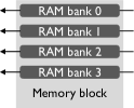
(a) RAM bank array

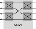
(b) Switching network

Figure 4: Two hardware blocks to implement particular types of SLPs. On the left, an array of $4$ RAM banks. Write and read addresses are used to delay differently elements. This block can be used to implement SLPs that do not permute across ports. On the right is an example of a switching network consisting of $4$ $2\!\times\!2$-switches. Switching networks can be used to implement SLPs that do not permute across time.

Conversely, SLPs that only permute across the ports within each cycle have the form

$$P=\begin{pmatrix}I_{m}&\\ P_{3}&P_{4}\end{pmatrix}.$$

They do not require memory and can be implemented using a network of $p_{3}\cdot 2^{n-1}$ $2\!\times\!2$-switches as was shown in [9]. This result, combined with decomposition (9) and Theorem 2 yields an immediate corollary:

Theorem 4.

For a given $P$, the associated SLP can be implemented using a RAM bank array (Fig. 4(a)) framed by two switching networks (Fig. 4(b)) with a total of $\max(p_{3},n+m-p_{4}-p_{1})\cdot 2^{n-1}$ $2\!\times\!2$-switches.

Our Algorithms 3 and 4, introduced later, provide an efficient method to compute this architecture.

3 Preliminaries

In this section, we will prove some basic lemmas that we will use throughout this article.

3.1 Properties of the blocks of an invertible matrix

In this subsection, we derive some direct consequences of the invertibility of $P$ on the range and the nullspace of its submatrices.

Lemma 2.

The following properties are immediate from the structure of $P$:

$$\ker P_{4}\cap\ker P_{2}=\{0\}$$ (11)

$$\ker P_{3}\cap\ker P_{1}=\{0\}$$ (12)

$$\operatorname{im}P_{4}+\operatorname{im}P_{3}=\mathbb{K}^{n}$$ (13)

$$\operatorname{im}P_{2}+\operatorname{im}P_{1}=\mathbb{K}^{m}$$ (14)

$$P_{3}(\ker P_{1})\cap P_{4}(\ker P_{2})=\{0\}$$ (15)

$$P_{1}(\ker P_{3})\cap P_{2}(\ker P_{4})=\{0\}$$ (16)

Proof.

We prove here equation (15). If $x\in\ker P_{1}$ and $y\in\ker P_{2}$ satisfy $P_{3}x=P_{4}y$, we have:

$$\begin{pmatrix}P_{1}&P_{2}\\ P_{3}&P_{4}\\ \end{pmatrix}\cdot\begin{pmatrix}x\\ -y\\ \end{pmatrix}=\begin{pmatrix}P_{1}x-P_{2}y\\ P_{3}x-P_{4}y\\ \end{pmatrix}=\begin{pmatrix}0\\ 0\\ \end{pmatrix}$$

Since $P$ is non-singular, $x=y=0$, as desired. ∎

These equalities yield the dimensions of the following subspaces:

Corollary 1.

$$\dim P_{2}(\ker P_{4})=\dim\ker P_{4}=n-p_{4}$$ (17)

$$\dim P_{1}(\ker P_{3})=\dim\ker P_{3}=m-p_{3}$$ (18)

$$\dim P_{4}(\ker P_{2})=\dim\ker P_{2}=n-p_{2}$$ (19)

$$\dim P_{3}(\ker P_{1})=\dim\ker P_{1}=m-p_{1}$$ (20)

$$\dim\operatorname{im}P_{4}\cap\operatorname{im}P_{3}=p_{4}+p_{3}-n$$ (21)

$$\dim\operatorname{im}P_{2}\cap\operatorname{im}P_{1}=p_{2}+p_{1}-m$$ (22)

Proof.

We prove equation (17). Since, by (11), $\ker P_{4}\cap\ker P_{2}=\{0\}$, the dimension of the image of $\ker P_{4}$ under $P_{2}$ has the same dimension as $\ker P_{4}$, which is $n-p_{4}$.

Equation (21) is a consequence of equation (13) and of the rank-nullity theorem. ∎

3.2 Algorithms on linear subspaces in matrix form

The algorithms we present in this article heavily rely on operations on subspaces of $\mathbb{K}^{m}$. To make the representation of these algorithms more practical for implementation, we introduce a matrix representation for subspaces and formulate the subspace operations needed in this paper on this representation.

We represent a linear subspace as an associated matrix whose columns form a basis of this subspace. In other words, if $\mathcal{A}$ is a subspace of $\mathbb{K}^{m}$ of dimension $n$, then we represent it using a $m\times n$ matrix $A$ such that $\operatorname{im}A=\mathcal{A}$. In this case, and only in this case, we will use the notation $\langle A\rangle=\operatorname{im}A$ to emphasize that the columns of $A$ form a linear independent set.

With this notation we can formulate subspace computations as computations on their associated matrices as explained in the following. To formally emphasize this correspondence, these operations on matrices will carry the same symbol as the subspace computation (e.g., $\cap$) they represent augmented with an overline (e.g., $\operatorname{\overline{\cap}}$). The operations are collected in Table 1. All algorithms in this paper are written as sequences of these matrix operations. Because of this, we implemented the algorithms by first designing an object oriented infrastructure that provides these operations. Then we could directly map the algorithms, as they are formulated, to code.

Operation related to subspaces	Associated matrix operation	Correspondence
Kernel of a matrix $M$	$\operatorname{\overline{\ker}}M$	$\langle\operatorname{\overline{\ker}}M\rangle=\ker M$
Direct sum of subspaces $\mathcal{A},\mathcal{B}$	$\begin{pmatrix}A&B\end{pmatrix}$	$\begin{pmatrix}A&B\end{pmatrix}=\mathcal{A}\oplus\mathcal{B}$
Intersection of subspaces $\mathcal{A},\mathcal{B}$	$A\operatorname{\overline{\cap}}B$	$\langle A\operatorname{\overline{\cap}}B\rangle=\mathcal{A}\cap\mathcal{B}$
Complement of a subspace $\mathcal{B}$ in $\mathcal{A}$	$A\operatorname{\overline{\ominus}}B$	$\langle A\operatorname{\overline{\ominus}}B\rangle\oplus\mathcal{B}=\mathcal{A}$

Table 1: We summarize matrix operators to perform basic operations on subspaces. $M$ is a general matrix, while $A$ and $B$ are matrices with $m$ rows that represent the subspaces $\mathcal{A}$ and $\mathcal{B}$; i.e. $\mathcal{A}=\langle A\rangle$ and $\mathcal{B}=\langle B\rangle$. Inspection of these routines shows that they all can be implemented with $O(m^{3})$ runtime.

Direct sum of two subspaces. If $\langle A\rangle,\langle B\rangle\leq\mathbb{K}^{m}$ are two subspaces, then the direct sum can be computed by concatenating the two matrices: $\langle A\rangle\oplus\langle B\rangle=\langle\begin{pmatrix}A&B\end{pmatrix}\rangle$.

Null space of a matrix. Gaussian elimination can be used to compute the null space of a given $m\times n$ matrix $M$. Indeed, if the reduced column echelon form of the matrix $\begin{pmatrix}M\\ I_{n}\end{pmatrix}$ is blocked into the form $\begin{pmatrix}M_{1}&\\ M_{3}&M_{4}\end{pmatrix},$ where $M_{1}$ has $m$ rows and no zero column, then $\ker M=\langle M_{4}\rangle$. We denote this computation with $\operatorname{\overline{\ker}}M=M_{4}$.

Intersection of two subspaces. For two subspaces $\operatorname{im}A,\operatorname{im}B\leq\mathbb{K}^{m}$, the intersection can be computed using the Zassenhaus algorithm. Namely, if the reduced column echelon form of $\begin{pmatrix}A&B\\ A&\end{pmatrix}$ is blocked into the form $\begin{pmatrix}C_{1}&&\\ C_{3}&C_{4}&\end{pmatrix},$ where $C_{1}$ and $C_{4}$ have $m$ rows and no zero column, then $\operatorname{im}A\cap\operatorname{im}B=\langle C_{4}\rangle$. We denote this computation with $A\operatorname{\overline{\cap}}B=C_{4}$.

Complement of a subspace within another one. Let $\operatorname{im}A\leq\operatorname{im}B\leq\mathbb{K}^{m}$. Then, a complement $\langle C\rangle$ of $\operatorname{im}A$ in $\operatorname{im}B$, i.e., a space that satisfies $\langle C\rangle\oplus\operatorname{im}A=\operatorname{im}B$, can be obtained as described in Algorithm 1. We denote this operation with $C=B\operatorname{\overline{\ominus}}A$.

Algorithm 1 Complement of a subspace within another

0:  Two matrices $A$ and $B$ with $m$ rows

0:  A matrix $A\operatorname{\overline{\ominus}}B$ such that $\langle A\operatorname{\overline{\ominus}}B\rangle\oplus\operatorname{im}B=\operatorname{im}A$

  $C\leftarrow$ A $m\times 0$ matrix

  for each column vector $b$ of $B$ do

     if $\operatorname{rk}\begin{pmatrix}A&C&b\end{pmatrix}>\operatorname{rk}\begin{pmatrix}A&C\end{pmatrix}$ then

        $C\leftarrow\begin{pmatrix}C&b\end{pmatrix}$

     end if

  end for

  return  $C$

3.3 Double complement

Lemma 3.

Let $\mathcal{C}$ be a finite-dimensional vector space and let $\mathcal{A},\mathcal{B}\leq\mathcal{C}$ with $\dim\mathcal{A}\geq\dim\mathcal{B}$. Then, there exists a space $\mathcal{S}\leq\mathcal{C}$ such that:

$$\left\{\begin{array}[]{l}\mathcal{S}\oplus\mathcal{A}=\mathcal{C}\\ \mathcal{S}\cap\mathcal{B}=\{0\}\end{array}\right.$$

Proof.

We first consider the case where $\mathcal{C}=\mathcal{A}+\mathcal{B}$. We denote with $\mathcal{P}$ (resp. $\mathcal{Q}$) a complement of $\mathcal{A}\cap\mathcal{B}$ in $\mathcal{A}$ (resp. in $\mathcal{B}$).

We show first that $\mathcal{P}\cap\mathcal{Q}=\{0\}$. Let $v\in\mathcal{P}\cap\mathcal{Q}$. As $\mathcal{P}\leq\mathcal{A}$ and $\mathcal{Q}\leq\mathcal{B}$, we have $v\in\mathcal{A}\cap\mathcal{B}$. Therefore, $v\in\mathcal{P}\cap\mathcal{A}\cap\mathcal{B}=\{0\},$ as desired.

We now denote with $b=\{b_{1},\dots,b_{p}\}$ (resp. $b^{\prime}=\{b^{\prime}_{1},\dots,b^{\prime}_{q}\}$) a basis of $\mathcal{P}$ (resp. $\mathcal{Q}$), implying $q\leq p$. Considering $w=\{b_{1}+b^{\prime}_{1},\dots,b_{q}+b^{\prime}_{q}\}$, the following holds:

$w$ is linear independent: if $\{\alpha_{1},\dots,\alpha_{q}\}\in\mathbb{K}^{q}$ is such that $\sum{\alpha_{i}w_{i}}=0$, then $\sum{\alpha_{i}b_{i}}=\sum{\alpha_{i}b^{\prime}_{i}}$. As $\sum{\alpha_{i}b_{i}}\in\mathcal{P}$ and $\sum{\alpha_{i}b^{\prime}_{i}}\in\mathcal{Q}$, it comes that $\sum\alpha_{i}b^{\prime}_{i}=\sum\alpha_{i}b_{i}=0$. It follows that for all $i$, $\alpha_{i}=0$, yielding the result.

$\langle w\rangle\cap\mathcal{A}=\{0\}$: If $v\in\langle w\rangle\cap\mathcal{A}$, then there exists $\{\alpha_{1},\dots,\alpha_{q}\}\in\mathbb{K}^{q}$ such that $v=\sum{\alpha_{i}(b_{i}+b^{\prime}_{i})}\in\mathcal{A}$. It implies $\sum{\alpha_{i}b^{\prime}_{i}}\in\mathcal{A}$. As the left hand side is in $\mathcal{Q}$, it comes that $\sum{\alpha_{i}b^{\prime}_{i}}=0$. It follows that for all $i$, $\alpha_{i}=0$, yielding the result.

$\langle w\rangle\cap\mathcal{B}=\{0\}$: Same proof as above.

Then, as $\dim\langle w\rangle=q=\dim\mathcal{C}-\dim\mathcal{A}$, $\mathcal{S}=\langle w\rangle$ satisfies the desired conditions.

In the general case, where $\mathcal{C}>\mathcal{A}+\mathcal{B}$, we use the same method, and simply add a complement $\mathcal{S}^{\prime}$ of $\mathcal{A}+\mathcal{B}$ in $\mathcal{C}$ to the solution.

∎

Algorithm 2 uses the method used in this proof to compute a basis of $\mathcal{S}$, given $\mathcal{A}$, $\mathcal{B}$ and $\mathcal{C}$. Note that if $\dim\mathcal{A}=\dim\mathcal{B}$, then $\mathcal{S}$ is a complement of both $\mathcal{A}$ and $\mathcal{B}$ in $\mathcal{C}$.

Algorithm 2 “Double complement” algorithm (Lemma 3)

0:  $A$, $B$ and $C$, such that $\operatorname{im}A,\operatorname{im}B\leq\operatorname{im}C$ and $\operatorname{rk}A\geq\operatorname{rk}B$

0:  A matrix $S$ such that $\langle S\rangle\oplus\operatorname{im}A=\operatorname{im}C$ and $\langle S\rangle\cap\operatorname{im}B=\{0\}$.

  $P\leftarrow A\operatorname{\overline{\ominus}}(A\operatorname{\overline{\cap}}B)$

  $Q\leftarrow B\operatorname{\overline{\ominus}}(A\operatorname{\overline{\cap}}B)$

  $P^{\prime}\leftarrow P$ truncated such that $P^{\prime}$ and $Q$ have the same size

  $S^{\prime}\leftarrow C\operatorname{\overline{\ominus}}\begin{pmatrix}A&B\end{pmatrix}$

  return  $\begin{pmatrix}S^{\prime}&P^{\prime}+Q\end{pmatrix}$

4 Proof of Theorem 1

We start with an auxiliary result that asserts that a decomposition of the form (3) is characterized by $L$.

Lemma 4.

Decomposition (3) exists if and only if $L$ is chosen such that $P_{4}-LP_{2}$ is non-singular. In this case,

$$\operatorname{rk}R=\operatorname{rk}(P_{3}-LP_{1}).$$ (23)

Proof.

We have:

$$\begin{pmatrix}I_{m}&\\ L&I_{n}\end{pmatrix}^{-1}P=\begin{pmatrix}P_{1}&P_{2}\\ P_{3}-LP_{1}&P_{4}-LP_{2}\end{pmatrix}$$ (24)

This matrix can be uniquely decomposed as in (2) if and only if $P_{4}-LP_{2}$ is non-singular, and we have the desired value for $\operatorname{rk}R$. ∎

Now we start the actual proof of Theorem 1. If we assume that decomposition (3) exists for $P$, then Lemma 4 yields

$$P=\begin{pmatrix}I_{m}&\\ L&I_{n}\end{pmatrix}\cdot\begin{pmatrix}P_{1}-P_{2}(P_{4}-LP_{2})^{-1}(P_{3}-LP_{1})&P_{2}\\ &P_{4}-LP_{2}\end{pmatrix}\cdot$$

$$\begin{pmatrix}I_{m}&\\ (P_{4}-LP_{2})^{-1}(P_{3}-LP_{1})&I_{n}\end{pmatrix}$$ (25)

It follows:

• (4) is obvious from (4).

• $\mathbb{K}^{n}=\operatorname{im}(P_{4}-LP_{2})\leq\operatorname{im}P_{4}+\operatorname{im}L$. Thus, $n\leq p_{4}+\operatorname{rk}L$, which yields (5).

• $\operatorname{im}(P_{3}-LP_{1})=(P_{3}-LP_{1})(\mathbb{K}^{n})\geq(P_{3}-LP_{1})(\ker P_{1})=P_{3}(\ker P_{1})$. (6) now follows from (20) and (23).

• (7) is a direct computation:

  $$\begin{array}[]{rcl}p_{3}&=&\operatorname{rk}(P_{3}-LP_{1}+LP_{1})\\ &\leq&\operatorname{rk}(P_{3}-LP_{1})+\operatorname{rk}(LP_{1})\\ &\leq&\operatorname{rk}R+\operatorname{rk}L.\end{array}$$

5 Proof of Theorem 2, case $p_{3}\leq m+n-p_{4}-p_{1}$

In this section, we provide an algorithm to construct an appropriate decomposition, in the case where $p_{3}\leq m+n-p_{4}-p_{1}$ (Figure 1 left). This means that, using Lemma 4, we have to build a matrix $L$ that satisfies

$$\begin{cases}P_{4}-LP_{2}\text{ is non-singular},\\ \operatorname{rk}L=n-p_{4},\\ \operatorname{rk}(P_{3}-LP_{1})=m-p_{1}.\end{cases}$$

5.1 Sufficient conditions

We first derive a set of sufficient conditions that ensure that $L$ satisfies the two following properties: $P_{4}-LP_{2}$ non singular (Lemma 5) and $\operatorname{rk}(P_{3}-LP_{1})=m-p_{1}$ (Lemma 6).

Lemma 5.

If $\operatorname{rk}L=n-p_{4}$ and $\operatorname{im}P_{4}\oplus LP_{2}(\ker P_{4})=\mathbb{K}^{n}$, then $P_{4}-LP_{2}$ is non-singular.

Proof.

We denote with $\mathcal{U}$ a complement of $\ker P_{4}$ in $\mathbb{K}^{n}$, i.e., $\mathbb{K}^{n}=\ker P_{4}\oplus\mathcal{U}$. This implies $\operatorname{im}P_{4}=P_{4}(\mathbb{K}^{n})=P_{4}(\mathcal{U})$. Now, let $\operatorname{im}P_{4}\oplus LP_{2}(\ker P_{4})=\mathbb{K}^{n}$. Hence, $\dim LP_{2}(\ker P_{4})=n-p_{4}=\operatorname{rk}L$ from which we get $\operatorname{im}L=LP_{2}(\ker P_{4})$. In particular, $LP_{2}(\mathcal{U})\leq\operatorname{im}L=LP_{2}(\ker P_{4})$. Further,

$$\begin{array}[]{rcl}\operatorname{im}(P_{4}-LP_{2})&=&(P_{4}-LP_{2})(\mathcal{U}\oplus\ker P_{4})\\ &=&(P_{4}-LP_{2})(\mathcal{U})+LP_{2}(\ker P_{4})\end{array}$$

As $LP_{2}(\mathcal{U})\leq LP_{2}(\ker P_{4})$ and $\operatorname{im}P_{4}\cap LP_{2}(\ker P_{4})=\{0\}$, we have:

$$\begin{array}[]{rcl}\operatorname{im}(P_{4}-LP_{2})&=&P_{4}(\mathcal{U})+LP_{2}(\ker P_{4})\\ &=&\operatorname{im}P_{4}+LP_{2}(\ker P_{4})\\ &=&\mathbb{K}^{n}\end{array}$$

as desired. ∎

Lemma 6.

If, for every vector $v$ of $\operatorname{im}P_{1}$, $L$ satisfies $Lv\in P_{3}P_{1}^{-1}(\{v\})$, then $\operatorname{rk}(P_{3}-LP_{1})=m-p_{1}$.

Proof.

Let $Lv\in P_{3}P_{1}^{-1}(\{v\})$ for all $v\in\operatorname{im}P_{1}$. If $u\in\mathbb{K}^{m}$, we have:

$$\begin{array}[]{rcl}(P_{3}-LP_{1})u&=&P_{3}u-LP_{1}u\\ &\in&P_{3}u-P_{3}P_{1}^{-1}(\{P_{1}u\})\\ &\in&P_{3}u-P_{3}(u+\ker P_{1})\\ &\in&P_{3}(\ker P_{1})\end{array}$$

Therefore, $\operatorname{im}(P_{3}-LP_{1})=P_{3}(\ker P_{1})$. Thus, $\operatorname{rk}P_{3}-LP_{1}=m-P_{1}$. ∎

The following lemma summarizes the two previous results:

Lemma 7.

Let $\mathcal{Y}$ be a complement of $\operatorname{im}P_{4}$ and $\mathcal{T}$ a complement of $P_{1}(\ker P_{3})$ in $\operatorname{im}P_{1}$. If

$$\begin{cases}\operatorname{im}L=\mathcal{Y},\\ L\cdot P_{2}(\ker P_{4})=\mathcal{Y},\\ L\cdot v\in P_{3}P_{1}^{-1}(\{v\}),\forall v\in\mathcal{T},\\ L\cdot P_{1}(\ker P_{3})=\{0\},\\ \end{cases}$$

then $L$ is an optimal solution.

5.2 Building $L$

We now build a matrix $L$ that satisfies the previous set of sufficient conditions. For all $v$ in a complement $\mathcal{T}$ of $P_{1}(\ker P_{3})$, $L$ has to satisfy $Lv\in P_{3}P_{1}^{-1}(\{v\})$. We first show that, given a suitable domain and image, it is possible to build a bijective linear mapping that satisfies this property.

Lemma 8.

Let $P_{1}(\ker P_{3})\oplus\mathcal{T}=\operatorname{im}P_{1}$ and $P_{3}(\ker P_{1})\oplus\mathcal{V}=\operatorname{im}P_{3}$. If

$$\mathcal{F}=P_{1}^{-1}(\mathcal{T})\cap P_{3}^{-1}(\mathcal{V}),$$

then the mapping $f:\mathcal{T}\rightarrow\mathcal{V}$ such that for all $v\in\mathcal{F},f(P_{1}v)=P_{3}v$ is well defined and is an isomorphism.

Proof.

We prove the lemma by first considering two functions $f_{1}$ and $f_{2}$ that are $P_{1}$ and $P_{3}$ restricted to $\mathcal{F}$ as shown in the diagram. We show that both are isomorphisms. Then $f=f_{2}\circ f_{1}^{-1}$ is the desired function.

We begin with the surjectivity of $f_{1}$. Let $x\in\mathcal{T}$. As $\mathcal{T}\leq\operatorname{im}P_{1}$, there exists a vector $v$ such that $P_{1}v=x$. The coset $v+\ker P_{1}$ is obviously a subset of $P_{1}^{-1}(\mathcal{T})$. Additionally, its image under $P_{3}$, the coset $P_{3}(v+\ker P_{1})=P_{3}v+P_{3}\ker P_{1}$ contains a unique representative $P_{3}v_{f}$ in $\mathcal{V}$, since $\operatorname{im}P_{3}=P_{3}(\ker P_{1})\oplus\mathcal{V}$. Therefore, $v_{f}\in P_{3}^{-1}(\mathcal{V})$, and thus $v_{f}\in\mathcal{F}$ and $f_{1}(v_{f})=x,$ as desired.

We now prove that $f_{1}$ is injective. Let $v\in\ker f_{1}\leq\mathcal{F}$. We have $P_{3}v\in\mathcal{V}$. Since $v\in\ker P_{1}$, $P_{3}v\in P_{3}\ker P_{1}$. Since $P_{3}(\ker P_{1})\cap\mathcal{V}=\{0\}$, $P_{3}v=0$ and thus $v\in\ker P_{3}$. Equation (12) shows that $v=0$, as desired. Thus, $f_{1}$ is bijective.

The proof that $f_{2}:\ \mathcal{F}\to\mathcal{V},\ v\mapsto P_{3}v$ is bijective is analogous. It follows that $f=f_{2}\circ f_{1}^{-1}$ is the desired isomorphism. ∎

As explained below, we now build a matrix $L$ that matches the conditions listed in Lemma 7. As they involve two spaces that may not be in a direct sum, $P_{2}(\ker P_{4})$ and a complement of $P_{1}(\ker P_{3})$ in $\operatorname{im}P_{1}$, some precautions must be taken.

We first construct the image $\mathcal{Y}$ of $L$. It must be a complement of $\operatorname{im}P_{4}$ and must contain a complement $\mathcal{Y}_{1}$ of $P_{3}(\ker P_{1})$ in $\operatorname{im}P_{3}$. As $p_{3}\leq m+n-p_{4}-p_{1}$, $m-p_{1}\geq p_{4}+p_{3}-n$, and we have $\dim(P_{3}(\ker P_{1}))\geq\dim(\operatorname{im}P_{4}\cap\operatorname{im}P_{3})$. Therefore, we can use the Lemma 3 to build a space $\mathcal{Y}_{1}$ such that:

$$\left\{\begin{array}[]{l}\mathcal{Y}_{1}\oplus P_{3}(\ker P_{1})=\operatorname{im}P_{3},\\ \mathcal{Y}_{1}\cap\operatorname{im}P_{4}\cap\operatorname{im}P_{3}=\{0\}.\end{array}\right.$$

We then complete $\mathcal{Y}_{1}$ to form a complement $\mathcal{Y}$ of $\operatorname{im}P_{4}$.

We now decompose $\mathbb{K}^{m}$ the following way:

We define $\mathcal{X}_{2}=P_{2}(\ker P_{4})\cap\operatorname{im}P_{1}$. $\mathcal{X}_{2}\cap P_{1}(\ker P_{3})=\{0\}$ according to equation (16). Then, we define $\mathcal{X}_{3}$ as a complement of $P_{1}(\ker P_{3})\oplus\mathcal{X}_{2}$ in $\operatorname{im}P_{1}$ and $\mathcal{X}_{1}$ as a complement of $\mathcal{X}_{2}$ in $P_{2}(\ker P_{4})$. $\mathcal{X}_{4}$ is defined as a complement of $\mathcal{X}_{1}\oplus\mathcal{X}_{2}\oplus\mathcal{X}_{3}\oplus P_{1}(\ker P_{3})$.

Finally, we build $L$ through the associated mapping, itself defined using a direct sum of linear mappings defined on the following subspaces of $\mathbb{K}^{m}$:

• We use Lemma 8 to construct a bijective linear mapping $f$ from $\mathcal{T}=\mathcal{X}_{2}\oplus\mathcal{X}_{3}$ over $\mathcal{Y}_{1}$. By definition, for all $v\in\mathcal{T}$, $f$ verifies $f(v)\in P_{3}P_{1}^{-1}(\{v\})$. Furthermore, as $f$ is bijective, its restriction on $\mathcal{X}_{2}$ is itself bijective over $f(\mathcal{X}_{2})$.

• We complete this bijective linear mapping with $g$, a bijective linear mapping between $\mathcal{X}_{1}$ and a complement $\mathcal{Y}_{2}$ of $f(\mathcal{X}_{2})$ in $\mathcal{Y}$. This way, the restriction of $f\oplus g$ on $\mathcal{X}_{1}\oplus\mathcal{X}_{2}=P_{2}(\ker P_{4})$ is bijective over $\mathcal{Y}$.

• We consider the mapping $h$ that maps $P_{1}(\ker P_{3})\oplus\mathcal{X}_{4}$ to $\{0\}$.

The matrix associated with the linear mapping $f\oplus g\oplus h$ satisfies all the conditions of Lemma 7, and is therefore an optimal solution.

This method is summarized in Algorithm 3, which allows us to construct a solution for Theorem 2. Its key part is the construction of a basis of $\mathcal{F}$, which uses a generalized pseudo-inverse $P_{1}^{\dagger}$ (resp. $P_{3}^{\dagger}$) of $P_{1}$ (resp. $P_{3}$), i.e., a matrix verifying $P_{1}P_{1}^{\dagger}P_{1}=P_{1}$ (resp. $P_{3}P_{3}^{\dagger}P_{3}=P_{3}$). This algorithm is a main contribution of this article.

Algorithm 3 Constructing $L$ (Theorem 2), case $p_{3}\leq m+n-p_{4}-p_{1}$

0:  $m$,$n$ and $P\in GL_{m+n}(\mathbb{K})$ such that $p_{3}\leq m+n-p_{4}-p_{1}$

0:  $L$

  $Y_{1}\leftarrow$ Alg. 2 with $A=P_{3}\cdot\operatorname{\overline{\ker}}P_{1}$, $B=P_{4}\operatorname{\overline{\cap}}P_{3}$, $C=P_{3}$

  $Y\leftarrow\begin{pmatrix}Y_{1}&I_{m}\operatorname{\overline{\ominus}}\begin{pmatrix}Y_{1}&P_{4}\end{pmatrix}\end{pmatrix}$

  $X_{2}\leftarrow(P_{2}\cdot\operatorname{\overline{\ker}}P_{4})\operatorname{\overline{\cap}}P_{1}$

  $X_{3}\leftarrow P_{1}\operatorname{\overline{\ominus}}\begin{pmatrix}(P_{1}\cdot\ker P_{3})&X_{2}\end{pmatrix})$

  $X_{1}\leftarrow(P_{2}\cdot\operatorname{\overline{\ker}}P_{4})\operatorname{\overline{\ominus}}X_{2}$

  $X_{4}\leftarrow I_{m}\operatorname{\overline{\ominus}}\begin{pmatrix}P_{1}&P_{2}\cdot\operatorname{\overline{\ker}}P_{4}\end{pmatrix}$

  $F\leftarrow\begin{pmatrix}\operatorname{\overline{\ker}}P_{1}&P_{1}^{\dagger}\cdot\begin{pmatrix}X_{2}&X_{3}\end{pmatrix}\end{pmatrix}\operatorname{\overline{\cap}}\begin{pmatrix}\operatorname{\overline{\ker}}P_{3}&P_{3}^{\dagger}\cdot Y_{1}\end{pmatrix}$

  $Y_{2}\leftarrow Y\operatorname{\overline{\ominus}}(P_{3}\cdot(\begin{pmatrix}\operatorname{\overline{\ker}}P_{1}&P_{1}^{\dagger}\cdot X_{2}\end{pmatrix}\operatorname{\overline{\cap}}F))$

  $L_{R}\leftarrow\begin{pmatrix}P_{1}\cdot F&X_{1}&P_{1}\cdot\operatorname{\overline{\ker}}P_{3}&X_{4}\end{pmatrix}$

  $L_{L}\leftarrow\begin{pmatrix}P_{3}\cdot F&Y_{2}&Z\end{pmatrix}$, where $Z$ is a zero filled matrix such that $L_{L}$ has the same number of columns as $L_{R}$

  return  $L_{L}\cdot L_{R}^{-1}$

Inspection of this algorithm shows that its arithmetic cost is $O((m+n)^{3})$.

5.3 Example

We illustrate our algorithm with a concrete example. Motivated by our main application (Section 2) we choose as base field $\mathbb{K}=\mathbb{F}_{2}$. For $m=4$ and $n=3$, we consider the matrix

$$P=\begin{pmatrix}P_{1}&P_{2}\\ P_{3}&P_{4}\\ \end{pmatrix}=\left(\begin{array}[]{cccc|ccc}1&1&&&1&&1\\ &&1&&&1&\\ 1&1&&1&1&1&1\\ &&&&&1&1\\ \hline\cr 1&&1&1&&&\\ 1&1&&&1&1&1\\ &1&&&&&\\ \end{array}\right).$$

We observe $p_{3}=3\leq m+n-p_{4}-p_{1}=4+3-1-3$. Therefore, we can use Algorithm 3 to compute a suitable $L$.

The first step is to compute $Y_{1}$. We have:

$$P_{3}\cdot\operatorname{\overline{\ker}}P_{1}=\begin{pmatrix}1\\ 0\\ 1\\ \end{pmatrix}\text{ and }P_{4}\operatorname{\overline{\cap}}P_{3}=\begin{pmatrix}0\\ 1\\ 0\\ \end{pmatrix}.$$

Using Algorithm 2, we get

$$Y_{1}=\begin{pmatrix}1&1\\ 1&0\\ 1&0\\ \end{pmatrix}.$$

Then, we complete it to form a complement of $\operatorname{\overline{\operatorname{im}}}P_{4}$:

$$Y=\begin{pmatrix}1&0\\ 0&1\\ 0&1\\ \end{pmatrix}.$$

The next step computes the different domains:

$$X_{2}=\begin{pmatrix}1\\ 1\\ 0\\ 0\\ \end{pmatrix}\text{, }X_{3}=\begin{pmatrix}1\\ 0\\ 0\\ 0\\ \end{pmatrix}\text{, }X_{1}=\begin{pmatrix}0\\ 0\\ 0\\ 1\\ \end{pmatrix}\text{ and }X_{4}=().$$

To compute $F$, we need pseudo-inverses of $P_{1}$ and $P_{2}$:

$$P_{1}^{\dagger}=\begin{pmatrix}0&0&0&0\\ 1&0&0&0\\ 0&1&0&0\\ 1&0&1&0\\ \end{pmatrix}\text{ and }P_{3}^{\dagger}=\begin{pmatrix}0&1&1\\ 0&0&1\\ 0&0&0\\ 1&1&1\\ \end{pmatrix}.$$

We then obtain:

$$F=\begin{pmatrix}0&0\\ 1&0\\ 0&1\\ 1&0\end{pmatrix}.$$

Then, we compute $Y_{2}$:

$$\mathcal{Y}_{2}=\begin{pmatrix}1\\ 0\\ 0\\ \end{pmatrix}.$$

Now we can compute $L$. With

$$L_{R}=\begin{pmatrix}1&0&0&0\\ 0&1&0&1\\ 0&0&0&1\\ 0&0&1&0\\ \end{pmatrix},L_{L}=\begin{pmatrix}1&1&1&0\\ 1&0&0&0\\ 1&0&0&0\\ \end{pmatrix}$$

we get

$$L=L_{L}\cdot L_{R}^{-1}=\begin{pmatrix}1&1&1&1\\ 1&0&0&0\\ 1&0&0&0\\ \end{pmatrix}.$$

The final decomposition is now obtained using (4):

$$P= \left(\begin{array}[]{cccc|ccc}1&&&&&&\\ &1&&&&&\\ &&1&&&&\\ &&&1&&&\\ \hline\cr 1&1&1&1&1&&\\ 1&&&&&1&\\ 1&&&&&&1\\ \end{array}\right)\cdot\left(\begin{array}[]{cccc|ccc}&1&&&1&&1\\ &&1&&&1&\\ &1&&1&1&1&1\\ 1&&&&&1&1\\ \hline\cr&&&&&1&1\\ &&&&&1&\\ &&&&1&&1\\ \end{array}\right)\cdot$$

$$\left(\begin{array}[]{cccc|ccc}1&&&&&&\\ &1&&&&&\\ &&1&&&&\\ &&&1&&&\\ \hline\cr&&&&1&&\\ &&&&&1&\\ 1&&&&&&1\\ \end{array}\right).$$

This decomposition satisfies $\operatorname{rk}L=2$ and $\operatorname{rk}R=1$, thus matching the bounds of Theorem 1.

If we consider the application presented in Section 2, this decomposition provides a way to implement in hardware the permutation associated with $P$ on $128$ elements, arriving in chunks of $8$ during $16$ cycles. This yields an implementation consisting of a permutation network of $4$ $2\!\times\!2$-switches, followed by a block of $8$ RAM banks, followed by another permutation network with $8$ $2\!\times\!2$-switches.

6 Proof of Theorem 2, case $p_{3}\geq m+n-p_{4}-p_{1}$

In this case, the third inequality in Theorem 1 is restrictive (Figure 1 right). Using again Lemma 4, we have to build a matrix $L$ satisfying:

$$\begin{cases}P_{4}-LP_{2}\text{ is non-singular}\\ \operatorname{rk}L=n-p_{4}\\ \operatorname{rk}(P_{3}-LP_{1})=p_{4}+p_{3}-n\end{cases}$$

As in the previous section, we will first provide a set of sufficient conditions for $L$ and then build it.

6.1 Sufficient conditions

The set of conditions that we will derive in this subsection will be slightly more complex than in the previous section, as we cannot reach the intrinsic bound of $\operatorname{rk}(P_{3}-LP_{1})$. Particularly, we cannot use Lemma 6 directly.

Lemma 9.

If $\mathcal{W}$ is such that $\mathcal{W}\oplus\operatorname{im}P_{4}=\mathbb{K}^{n}$ and $\mathcal{T}$ is such that:

$$\left\{\begin{array}[]{l}\mathcal{T}\cap P_{1}(\ker P_{3})=\{0\}\\ \mathcal{T}\leq\operatorname{im}P_{1}\\ \dim\mathcal{T}=n-p_{4},\\ \end{array}\right.$$

then if $L$ satisfies

$$\left\{\begin{array}[]{l}\operatorname{im}L=\mathcal{W}\\ L\cdot P_{2}(\ker P_{4})=\mathcal{W}\\ L\cdot v\in P_{3}P_{1}^{-1}(\{v\}),\forall v\in\mathcal{T}\\ L\cdot P_{1}(\ker P_{3})=\{0\}\\ \end{array}\right.$$

then $L$ is a solution that verifies $\operatorname{rk}L=n-p_{4}$ and $\operatorname{rk}(P_{3}-LP_{1})=p_{4}+p_{3}-n$.

Proof.

Let $L$ be a matrix that satisfies the conditions above. Using Lemma 5 as before, we get that $\operatorname{rk}L=n-p_{4}$ and $P_{4}-LP_{2}$ invertible.

Now, with the definition of $\mathcal{T}$, we can define a dimension $p_{4}+p_{3}+p_{1}-m-n$ space $\mathcal{T^{\prime}}$ such that $\operatorname{im}P_{1}=P_{1}(\ker P_{3})\oplus\mathcal{T}\oplus\mathcal{T^{\prime}}$. Then, we define a matrix $L^{\prime}$ such that:

$$\left\{\begin{array}[]{l}L^{\prime}\cdot v\in Lv-P_{3}P_{1}^{-1}(\{v\})\text{, for all }v\in\mathcal{T^{\prime}}\\ L^{\prime}\cdot v=0\text{, for all $v$ in $P_{1}(\ker P_{3})\oplus\mathcal{T}$}\\ L^{\prime}\cdot v=0\text{, for all $v$ in a complement of $\operatorname{im}P_{1}$},\\ \end{array}\right.$$

$L^{\prime}$ is therefore a rank $p_{4}+p_{3}+p_{1}-m-n$ matrix such that $\text{for all }v\in\operatorname{im}P_{1},(L-L^{\prime})v\in P_{3}P_{1}^{-1}(\{v\})$. We apply Lemma 6 on $L-L^{\prime}$ and get:

$$\begin{array}[]{rcl}\operatorname{rk}(P_{3}-LP_{1})&=&\operatorname{rk}(P_{3}-(L-L^{\prime})P_{1}-L^{\prime}P_{1})\\ &\leq&\operatorname{rk}(P_{3}-(L-L^{\prime})P_{1})+\operatorname{rk}(L^{\prime}P_{1})\\ &\leq&\dim P_{3}(\ker P_{1})+\operatorname{rk}L^{\prime}\\ &\leq&p_{4}+p_{3}-n,\\ \end{array}$$

as desired. ∎

6.2 Building $L$

We will build a matrix $L$ that matches the conditions listed in Lemma 9. As before, we consider the image $\mathcal{Y}$ of $L$ first. We will design it such that it is a complement of $\operatorname{im}P_{4}$, and that is contained in a complement $\mathcal{Y^{\prime}}$ of $P_{3}(\ker P_{1})$ in $\operatorname{im}P_{3}$. Using $p_{3}\geq m+n-p_{4}-p_{1}$ and Lemma 3, we can get a space $\mathcal{Y}$ such that:

$$\left\{\begin{array}[]{l}\mathcal{Y}\oplus(\operatorname{im}P_{4}\cap\operatorname{im}P_{3})=\operatorname{im}P_{3}\\ \mathcal{Y}\cap P_{3}(\ker P_{1})=\{0\}\end{array}\right.$$

This space satisfies $\mathcal{Y}\oplus\operatorname{im}P_{4}=\operatorname{im}P_{3}+\operatorname{im}P_{4}=\mathbb{K}^{n}$, and can be completed to a complement $\mathcal{Y^{\prime}}$ of $P_{3}(\ker P_{1})$ in $\operatorname{im}P_{3}$. Note that we will use $\mathcal{Y^{\prime}}$ only to define $f$; the image of $L$ will be $\mathcal{Y}$.

Now, as before, we build $L$ through the associated mapping, itself defined using a direct sum of linear mappings defined on the same subspaces of $\mathbb{K}^{m}$ as in Section 5.2.

• We use Lemma 8 to construct a first bijective linear mapping $f^{\prime}$ between $\mathcal{T^{\prime}}=\mathcal{X}_{2}\oplus\mathcal{X}_{3}$ and $\mathcal{Y^{\prime}}$. As $f^{\prime}$ is bijective, we can define $\mathcal{T}=f^{\prime-1}(\mathcal{Y})$ and $f=\mathchoice{{f^{\prime}\,\smash{\vrule height=6.80002pt,depth=1.65279pt}}_{\,\mathcal{T}}}{{f^{\prime}\,\smash{\vrule height=6.80002pt,depth=1.65279pt}}_{\,\mathcal{T}}}{{f^{\prime}\,\smash{\vrule height=4.77779pt,depth=1.16167pt}}_{\,\mathcal{T}}}{{f^{\prime}\,\smash{\vrule height=3.66667pt,depth=1.16167pt}}_{\,\mathcal{T}}}$. Thus, $\mathcal{T}$ satisfies the properties in Lemma 9 and $L$ the condition for all $v\in\mathcal{T},Lv\in P_{3}P_{1}^{-1}(\{v\})$.

• Then, we consider a complement $\mathcal{X}_{1}^{\prime}$ of $\mathcal{T}\cap\mathcal{X}_{2}$ in $P_{2}(\ker P_{4})$, a complement $\mathcal{Y}_{2}^{\prime}$ of $f(\mathcal{T}\cap\mathcal{X}_{2})$ in $\mathcal{Y}$ and a bijective linear mapping $g$ between $\mathcal{X}_{1}^{\prime}$ and $\mathcal{Y}_{2}^{\prime}$. This way, the restriction of $f\oplus g$ on $P_{2}(\ker P_{4})$ is bijective over $\mathcal{Y}$.

The rest of the algorithm in similar to the previous case:

• We consider the mapping $h$ that maps $P_{1}(\ker P_{3})$ to $\{0\}$.

• To complete the definition of $L$, we take a mapping $h^{\prime}$ between a complement $\mathcal{X}_{4}^{\prime}$ of $\mathcal{X}_{1}^{\prime}\oplus\mathcal{T}\oplus P_{1}(\ker P_{3})$ and $\{0\}$.

The matrix associated with the mapping $f\oplus g\oplus h\oplus h^{\prime}$ satisfies all the conditions of Lemma 9, and is therefore an optimal solution.

Algorithm 4 summarizes this method, and allows to construct a solution for Theorem 2, in the case where $p_{3}>m+n-p_{4}-p_{1}$. This algorithm is a main contribution of this article.

Algorithm 4 Constructing $L$ (Theorem 2), case $p_{3}>m+n-p_{4}-p_{1}$

0:  $m$,$n$, $P\in GL_{m+n}(\mathbb{K})$ such that $p_{3}>m+n-p_{4}-p_{1}$

0:  $L$

  $Y\leftarrow$ Alg. 2 with $A=P_{4}\operatorname{\overline{\cap}}P_{3}$, $B=P_{3}\cdot\operatorname{\overline{\ker}}P_{1}$ and $C=P_{3}$

  $X_{2}\leftarrow(P_{2}\cdot\operatorname{\overline{\ker}}P_{4})\operatorname{\overline{\cap}}P_{1}$

  $X_{3}\leftarrow P_{1}\operatorname{\overline{\ominus}}\begin{pmatrix}P_{1}\cdot\operatorname{\overline{\ker}}P_{3}&X_{2}\end{pmatrix}$

  $F\leftarrow\begin{pmatrix}\operatorname{\overline{\ker}}P_{1}&P_{1}^{\dagger}\cdot\begin{pmatrix}X_{2}&X_{3}\end{pmatrix}\end{pmatrix}\operatorname{\overline{\cap}}\begin{pmatrix}\operatorname{\overline{\ker}}P_{3}&P_{3}^{\dagger}\cdot Y\end{pmatrix}$

  $X_{1}^{\prime}\leftarrow(P_{2}\cdot\ker P_{4})\operatorname{\overline{\ominus}}((P_{1}\cdot F)\operatorname{\overline{\cap}}X_{2})$

  $X_{4}\leftarrow I_{m}\operatorname{\overline{\ominus}}\begin{pmatrix}X^{\prime}_{1}&P_{1}\cdot F&P_{1}\cdot\operatorname{\overline{\ker}}P_{3}\end{pmatrix}$

  $Y_{2}^{\prime}\leftarrow Y\operatorname{\overline{\ominus}}(P_{3}\cdot(F\operatorname{\overline{\cap}}\begin{pmatrix}P_{1}^{\dagger}\cdot X_{2}&\operatorname{\overline{\ker}}P_{1}\end{pmatrix}))$

  $L_{R}\leftarrow\begin{pmatrix}P_{1}\cdot F&X^{\prime}_{1}&P_{1}\cdot\operatorname{\overline{\ker}}P_{3}&X_{4}\end{pmatrix}$

  $L_{L}\leftarrow\begin{pmatrix}P_{3}\cdot F&Y^{\prime}_{2}&Z\end{pmatrix}$, where $Z$ is a zero filled matrix such that $L_{L}$ has the same number of columns as $L_{R}$

  return  $L_{L}\cdot L_{R}^{-1}$

As in the previous case, this algorithm has an arithmetic cost cubic in $m+n$.

6.3 Example

We now consider, for $\mathbb{K}=\mathbb{F}_{2}$, $m=4$ and $n=3$, the matrix

$$P=\begin{pmatrix}P_{1}&P_{2}\\ P_{3}&P_{4}\\ \end{pmatrix}=\left(\begin{array}[]{cccc|ccc}&1&1&1&1&&\\ 1&&&1&&1&1\\ &1&1&1&&1&1\\ 1&1&&1&&1&1\\ \hline\cr 1&&&1&&1&\\ &&&1&&1&\\ 1&&1&1&1&1&\\ \end{array}\right).$$

We observe $p_{3}=3>m+n-p_{4}-p_{1}=4+3-2-3$. Therefore, we use Algorithm 4 to compute a suitable $L$.

The first step is to compute $Y$. We have:

$$P_{3}\cdot\operatorname{\overline{\ker}}P_{1}=\begin{pmatrix}0\\ 1\\ 1\\ \end{pmatrix}\text{ and }P_{4}\operatorname{\overline{\cap}}P_{3}=\begin{pmatrix}0\\ 1\\ 0\\ \end{pmatrix}.$$

Using Algorithm 2, we get

$$Y_{1}=\begin{pmatrix}1&1\\ 1&0\\ 1&0\\ \end{pmatrix}.$$

Then, we complete it to form a complement of $\operatorname{im}P_{4}$:

$$Y=\begin{pmatrix}1&0\\ 1&0\\ 0&1\\ \end{pmatrix}.$$

The next step computes the different domains:

$$X_{2}=()\text{ and }X_{3}=\begin{pmatrix}1&0\\ 0&1\\ 1&0\\ 0&0\\ \end{pmatrix}.$$

To compute $F$, we need pseudo-inverses of $P_{1}$ and $P_{2}$:

$$P_{1}^{\dagger}=\begin{pmatrix}0&0&0&0\\ 0&1&0&1\\ 0&0&1&1\\ 0&1&0&0\\ \end{pmatrix}\text{ and }P_{3}^{\dagger}=\begin{pmatrix}1&1&0\\ 0&0&0\\ 1&0&1\\ 0&1&0\\ \end{pmatrix}$$

and get

$$F=\begin{pmatrix}1\\ 1\\ 0\\ 0\end{pmatrix}.$$

Next we compute the remaining subspaces that depend on $F$:

$$X_{1}^{\prime}=\begin{pmatrix}0\\ 1\\ 1\\ 1\end{pmatrix}\text{, }X_{4}=\begin{pmatrix}1\\ 0\\ 0\\ 0\end{pmatrix}\text{, and }Y_{2}^{\prime}=\begin{pmatrix}1\\ 0\\ 1\end{pmatrix}.$$

Noe we can compute $L$. With

$$L_{R}=\begin{pmatrix}1&0&1&1\\ 1&1&0&0\\ 1&1&1&0\\ 0&1&1&0\\ \end{pmatrix},L_{L}=\begin{pmatrix}1&1&0&0\\ 0&0&0&0\\ 1&1&0&0\\ \end{pmatrix}$$

we get

$$L=L_{L}\cdot L_{R}^{-1}=\begin{pmatrix}0&1&0&0\\ 0&0&0&0\\ 0&1&0&0\\ \end{pmatrix}.$$

The final decomposition is obtained using (4):

$$P= \left(\begin{array}[]{cccc|ccc}1&&&&&&\\ &1&&&&&\\ &&1&&&&\\ &&&1&&&\\ \hline\cr&1&&&&&\\ &&&&&&\\ &1&&&&&\\ \end{array}\right)\cdot\left(\begin{array}[]{cccc|ccc}&1&&1&1&&\\ 1&&&&&1&1\\ &1&1&&&1&1\\ 1&1&&&&1&1\\ \hline\cr&&&&&&1\\ &&&&&1&\\ &&&&1&&1\\ \end{array}\right)\cdot$$

$$\left(\begin{array}[]{cccc|ccc}1&&&&&&\\ &1&&&&&\\ &&1&&&&\\ &&&1&&&\\ \hline\cr&&1&&1&&\\ &&&1&&1&\\ &&&&&&1\\ \end{array}\right).$$

This decomposition satisfies $\operatorname{rk}L=1$ and $\operatorname{rk}R=2$, thus matching the bounds of Theorem 1.

As before, if we consider the application of Section 2. The decomposition shows that we can implement in hardware the permutation associated with $P$ on $128$ elements, arriving in chunks of $8$ during $16$ cycles through a permutation network of $8$ $2\!\times\!2$-switches, followed by a block of $8$ RAM banks, followed by another permutation network with $4$ $2\!\times\!2$-switches.

7 Rank exchange

The solution built in Section 6.2 satisfies $\operatorname{rk}L=n-p_{4}$ and $\operatorname{rk}P_{3}-LP_{1}=p_{4}+p_{3}-n$. In this section, we will show that it is possible to construct a solution for all possible pairs $(\operatorname{rk}L,\operatorname{rk}P_{3}-LP_{1})$ matching the bounds in Theorem 1. First, we will construct a rank $1$ matrix $L^{\prime}$ that will trade a rank of $L$ for a rank of $P_{3}-LP_{1}$ (i.e., $\operatorname{rk}(L+L^{\prime})=1+\operatorname{rk}L$, $\operatorname{rk}(P_{3}-(L+L^{\prime})P_{1})=\operatorname{rk}(P_{3}-LP_{1})-1$ and $P_{4}-(L+L^{\prime})P_{2}$ is non-singular) (see Figure 5). This method can then be applied several times, until $\operatorname{rk}(P_{3}-LP_{1})$ reaches its own bound, $m-p_{1}$.

Figure 5: $L^{\prime}$ trades a rank of $L$ for a rank of $R$ on the associated decomposition.

We assume that $L$ satisfies the following conditions:

$$\left\{\begin{array}[]{l}P_{4}-LP_{2}\text{ is non-singular}\\ \operatorname{rk}L+\operatorname{rk}(P_{3}-LP_{1})=p_{3}\\ \operatorname{rk}(P_{3}-LP_{1})>m-p_{1}\end{array}\right.$$

As in the previous sections, we first formulate sufficient conditions on $L^{\prime}$, before building it.

7.1 Sufficient conditions

We now define $C=P_{1}-P_{2}(P_{4}-LP_{2})^{-1}(P_{3}-LP_{1})$.

Lemma 10.

If $z\in\mathbb{K}^{m}$ satisfies $z\notin\ker(P_{3}-LP_{1})+\ker P_{1}$ and $L^{\prime}$ satisfies:

$$\left\{\begin{array}[]{l}\operatorname{rk}L^{\prime}=1\\ L^{\prime}P_{1}\ker(P_{3}-LP_{1})=\{0\}\\ L^{\prime}P_{1}z=(P_{3}-LP_{1})z\\ L^{\prime}Cz\neq 0\end{array}\right.$$

Then $L+L^{\prime}$ is an optimal solution to our problem that satisfies $\operatorname{rk}(P_{3}-(L+L^{\prime})P_{1})=\operatorname{rk}(P_{3}-LP_{1})-1$.

Proof.

We first prove that $P_{4}-(L+L^{\prime})P_{2}=(I-L^{\prime}P_{2}(P_{4}-LP_{2})^{-1})(P_{4}-LP_{2})$ is non singular. Let $x\in\ker(I-L^{\prime}P_{2}(P_{4}-LP_{2})^{-1})$. $x$ satisfies:

$$x-L^{\prime}P_{2}(P_{4}-LP_{2})^{-1}x=0.$$

Therefore, $x\in\operatorname{im}L^{\prime}$. As $\operatorname{rk}L^{\prime}=1$, $\exists\lambda\in\mathbb{K}$, $x=\lambda(P_{3}-LP_{1})z=\lambda L^{\prime}P_{1}z$. It comes that

$$\lambda L^{\prime}P_{1}z-\lambda L^{\prime}P_{2}(P_{4}-LP_{2})^{-1}(P_{3}-LP_{1})z=0.$$

Finally, $\lambda L^{\prime}Cz=0$, which implies, as $L^{\prime}Cz\neq 0$, $\lambda=0$, as desired.

We now prove that $\operatorname{rk}(P_{3}-(L+L^{\prime})P_{1})=\operatorname{rk}(P_{3}-LP_{1})-1$. We have already $\ker(P_{3}-(L+L^{\prime})P_{1})\leq\ker(P_{3}-LP_{1})$ as $L^{\prime}P_{1}\ker(P_{3}-LP_{1})=\{0\}$. We also have $(P_{3}-(L^{\prime}+L)P_{1})z=0$. As $z\notin\ker(P_{3}-LP_{1})+\ker P_{1}$, $\ker(P_{3}-(L+L^{\prime})P_{1})\geq\ker(P_{3}-LP_{1})\oplus\langle z\rangle$. Therefore,

$$\dim\ker(P_{3}-(L+L^{\prime})P_{1})\geq 1+\dim\ker(P_{3}-LP_{1}),$$

as desired. ∎

7.2 Building $L^{\prime}$

Lemma 11.

$\ker(P_{3}-LP_{1})\cap\ker P_{1}=\{0\}$

Proof.

This is a consequence of (24): the block column $\begin{pmatrix}P_{1}\\ P_{3}-LP_{1}\end{pmatrix}$ has full rank. ∎

Thus, we have $\dim(\ker(P_{3}-LP_{1})\oplus\ker P_{1})=2m-p_{1}-\operatorname{rk}(P_{3}-LP_{1})<m$. Decomposition (4) shows that $C$ is non-singular, and we have $\dim C^{-1}P_{1}\ker(P_{3}-LP_{1})=\dim P_{1}\ker(P_{3}-LP_{1})=\dim\ker(P_{3}-LP_{1})=m-\operatorname{rk}(P_{3}-LP_{1})$. Using Lemma 3, we can build a space $\mathcal{Z}$ such that:

$$\left\{\begin{array}[]{l}\mathcal{Z}\oplus\ker(P_{3}-LP_{1})\oplus\ker P_{1}=\mathbb{K}^{m}\\ \mathcal{Z}\cap C^{-1}P_{1}\ker(P_{3}-LP_{1})=\{0\}\end{array}\right.$$

We can now pick a nonzero element $z\in\mathcal{Z}$ and build a corresponding $L^{\prime}$:

• If $Cz\in P_{1}\ker(P_{3}-LP_{1})\oplus\langle P_{1}z\rangle$: We take a complement $\mathcal{A}$ of $P_{1}\ker(P_{3}-LP_{1})\oplus\langle P_{1}z\rangle$ and build $L^{\prime}$ such that:

  $$\left\{\begin{array}[]{l}L^{\prime}P_{1}z=(P_{3}-LP_{1})z\\ L^{\prime}(P_{1}\ker(P_{3}-LP_{1})\oplus\mathcal{A})=\{0\}\\ \end{array}\right.$$

  We have $L^{\prime}Cz\neq 0$. In fact, $Cz$ can be uniquely decomposed in the form $k+\lambda P_{4}z$, where $k\in P_{1}\ker(P_{3}-LP_{1})$ and $\lambda\in\mathbb{K}$. As $z\notin C^{-1}P_{1}\ker(P_{3}-LP_{1})$, $\lambda\neq 0$. Then, $L^{\prime}Cz=L^{\prime}k+L^{\prime}\lambda P_{4}z=0+\lambda(P_{3}-LP_{1})z\neq 0$.

• If $Cz\notin P_{1}\ker(P_{3}-LP_{1})\oplus\langle P_{1}z\rangle$: The vector $a=Cz-P_{1}z$ is outside of $P_{1}\ker(P_{3}-LP_{1})\oplus\langle P_{1}z\rangle$. Therefore, it is possible to build a complement $\mathcal{A}$ of $P_{1}\ker(P_{3}-LP_{1})\oplus\langle P_{1}z\rangle$ that contains $a$. Then, we build $L^{\prime}$ as before:

  $$\left\{\begin{array}[]{l}L^{\prime}P_{1}z=(P_{3}-LP_{1})z\\ L^{\prime}(P_{1}\ker(P_{3}-LP_{1})\oplus\mathcal{A})=\{0\}\\ \end{array}\right.$$

  As in the previous case, we have $L^{\prime}Cz=L^{\prime}a+L^{\prime}P_{1}z=0+(P_{3}-LP_{1})z\neq 0$.

In both cases, the matrix $L^{\prime}$ we built satisfies the conditions of Lemma 10. Therefore, $L+L^{\prime}$ is the desired solution.

Algorithm 5 summarizes this method, and allows to build a new optimal solution from a pre-existing one, with a different trade-off. This algorithm is a main contribution of this article.

Algorithm 5 Exchanging ranks between $L$ and $R$ (Theorem 3)

0:  $P$ and a solution $L$ such that $\operatorname{rk}(P_{3}-LP_{1})>m-p_{1}$

0:  A new optimal solution $L$ with a rank incremented by $1$

  $K\leftarrow\operatorname{\overline{\ker}}(P_{3}-LP_{1})$

  $C\leftarrow P_{1}-P_{2}(P_{4}-LP_{2})^{-1}(P_{3}-LP_{1})$

  $Z\leftarrow$ Alg. 2 with $A=\begin{pmatrix}K&\operatorname{\overline{\ker}}P_{1}\end{pmatrix},B=C^{-1}P_{1}K$ and $C=I_{m}$

  $z\leftarrow$ first column of $Z$

  if $Cz\in\begin{pmatrix}P_{1}\cdot K&P_{1}z\end{pmatrix}$ then

     $A\leftarrow I_{m}\operatorname{\overline{\ominus}}P_{1}\cdot\begin{pmatrix}K&z\end{pmatrix}$

  else

     $a\leftarrow(C-P_{1})z$

     $A\leftarrow\begin{pmatrix}I_{m}\operatorname{\overline{\ominus}}\begin{pmatrix}P_{1}K&P_{1}z&a\end{pmatrix}&a\end{pmatrix}$

  end if

  $L^{\prime}_{R}\leftarrow\begin{pmatrix}P_{1}z&P_{1}K&A\end{pmatrix}$

  $L^{\prime}_{L}\leftarrow\begin{pmatrix}(P_{3}-LP_{1})z&F\end{pmatrix}$, where $F$ is a zero filled matrix such that $L^{\prime}_{L}$ has the same number of columns as $L^{\prime}_{R}$

  return  $L+L^{\prime}_{L}\cdot L_{R}^{\prime-1}$

7.3 Example

To illustrate Algorithm 5, we continue the example of Section 6.3, and the matrix $L$ that we found. We have:

$$K=\begin{pmatrix}1&0\\ 0&1\\ 0&0\\ 0&0\\ \end{pmatrix}\text{ and }C=\begin{pmatrix}&1&&1\\ 1&&&\\ &1&1&\\ 1&1&&\\ \end{pmatrix}.$$

Using Algorithm 2, we get

$$Z=z=\begin{pmatrix}0\\ 0\\ 1\\ 0\end{pmatrix}.$$

As $Cz=\begin{pmatrix}0\\ 0\\ 1\\ 0\end{pmatrix}$ is not included in $\begin{pmatrix}P_{1}K&P_{1}z\end{pmatrix}=\begin{pmatrix}1&0&0\\ 0&1&0\\ 1&0&0\\ 0&0&1\\ \end{pmatrix}$, we compute $A$ as a complement of $\begin{pmatrix}P_{1}K&P_{1}z\end{pmatrix}$ that contains $a=\begin{pmatrix}1\\ 0\\ 0\\ 0\\ \end{pmatrix}$:

$$\mathcal{A}=\left\langle\begin{pmatrix}1\\ 0\\ 0\\ 0\\ \end{pmatrix}\right\rangle.$$

Now, we compute $L^{\prime}$, using:

$$L^{\prime}_{R}=\begin{pmatrix}1&0&1&1\\ 0&1&0&0\\ 1&0&1&0\\ 0&1&1&0\\ \end{pmatrix}\text{, }L^{\prime}_{L}=\begin{pmatrix}0&0&0&0\\ 0&0&0&0\\ 1&0&0&0\\ \end{pmatrix}\text{, and }L^{\prime}=\begin{pmatrix}0&0&0&0\\ 0&0&0&0\\ 0&1&1&1\\ \end{pmatrix}.$$

Finally, we get the new decomposition, using, as usual, Equation (4):

$$P= \left(\begin{array}[]{cccc|ccc}1&&&&&&\\ &1&&&&&\\ &&1&&&&\\ &&&1&&&\\ \hline\cr&1&&&1&&\\ &&&&&1&\\ &&1&1&&&1\\ \end{array}\right)\cdot\left(\begin{array}[]{cccc|ccc}&1&1&1&1&&\\ 1&&&&&1&1\\ &1&1&&&1&1\\ 1&1&&&&1&1\\ \hline\cr&&&&&&1\\ &&&&&1&\\ &&&&1&1&\\ \end{array}\right)\cdot$$

$$\left(\begin{array}[]{cccc|ccc}1&&&&&&\\ &1&&&&&\\ &&1&&&&\\ &&&1&&&\\ \hline\cr&&&&1&&\\ &&&1&&1&\\ &&&&&&1\\ \end{array}\right).$$

As expected, the left off-diagonal rank has increased by one, while the right one has decreased by one. The two different decompositions that we now have for $P$ cover all the possible tradeoffs that minimize the off-diagonal ranks.

8 Conclusion

In this paper, we introduced a novel block matrix decomposition that generalizes the classical block-LU factorization. A $2\!\times\!2$-blocked invertible matrix is decomposed into a product of three matrices: lower block unitriangular, upper block triangular, and lower block unitriangular matrix, such that the sum of the off-diagonal ranks are minimal. We provided an algorithm that computes an optimal solution with an asympotic number of operations cubic in the matrix size. We note that we implemented the algorithm for finite fields, for rational numbers, for Gaussian rational numbers and for exact real arithmetic for validation. For a floating point implementation, numerical issues may arise.

The origin of the considered decomposition, as we explained, is in the design of optimal circuits for a certain class of streaming permutations that are very relevant in practice. However, we believe that because of its simple and natural structure, the matrix decomposition is also of pure mathematical interest. Specifically, it would be interesting to investigate if the proposed decomposition is a special case of a more general problem that involves, for example, finer block structures.

References

• [1] D.ย Carlson, E.ย Haynsworth, and T.ย Markham. A generalization of the Schur complement by means of the Moore-Penrose inverse. SIAM Journal on Applied Mathematics, 26(1):169โ€“175, 1974.
• [2] E.ย Chow and Y.ย Saad. Approximate inverse techniques for block-partitioned matrices. SIAM Journal on Scientific Computing, 18(6):1657โ€“1675, 1997.
• [3] Richardย W. Cottle. Manifestations of the Schur complement. Linear Algebra and its Applications, 8(3):189 โ€“ 211, 1974.
• [4] Jamesย W. Demmel, Nicholasย J. Higham, and Robertย S. Schreiber. Block LU factorization. Numerical Linear Algebra with Applications, 2(2):173โ€“190, 1992.
• [5] Jacques Lenfant and Serge Tahรฉ. Permuting data with the Omega network. Acta Informatica, 21(6):629โ€“641, 1985.
• [6] Victor Pan. Structured matrices and polynomials: unified superfast algorithms. Springer Science & Business Media, 2001.
• [7] Keshabย K. Parhi. Systematic synthesis of DSP data format converters using life-time analysis and forward-backward register allocation. IEEE Transactions on Circuits and Systems II: Analog and Digital Signal Processing, 39(7):423โ€“440, Jul 1992.
• [8] Marshallย C. Pease. The indirect binary n-cube microprocessor array. IEEE Transactions on Computers, 26(5):458โ€“473, May 1977.
• [9] Markus Pรผschel, Peterย A. Milder, and Jamesย C. Hoe. Permuting streaming data using RAMs. Journal of the ACM, 56(2):10:1โ€“10:34, 2009.
• [10] R.ย Tolimieri, M.ย An, and C.ย Lu. Algorithms for Discrete Fourier Transforms and Convolution. Springer, 2nd edition, 1997.
• [11] Fuzhen Zhang. The Schur Complement and its Applications, volumeย 4. Springer, 2006.