A new correction of stellar oscillation frequencies for near-surface effects

Abstract

Context. Space-based observations of solar-like oscillations present an opportunity to constrain stellar models using individual mode frequencies. However, current stellar models are inaccurate near the surface, which introduces a systematic difference that must be corrected.

Aims. We introduce and evaluate two parametrizations of the surface corrections based on formulae given by Gough (1990). The first we call a cubic term proportional to $\nu^{3}/\mathcal{I}$ and the second has an additional inverse term proportional to $\nu^{-1}/\mathcal{I}$, where $\nu$ and $\mathcal{I}$ are the frequency and inertia of an oscillation mode.

Methods. We first show that these formulae accurately correct model frequencies of two different solar models (Model S and a calibrated MESA model) when compared to observed BiSON frequencies. In particular, even the cubic form alone fits significantly better than a power law. We then incorporate the parametrizations into a modelling pipeline that simultaneously fits the surface effects and the underlying stellar model parameters. We apply this pipeline to synthetic observations of a Sun-like stellar model, solar observations degraded to typical asteroseismic uncertainties, and observations of the well-studied CoRoT target HD 52265. For comparison, we also run the pipeline with the scaled power-law correction proposed by Kjeldsen et al. (2008).

Results. The fits to synthetic and degraded solar data show that the method is unbiased and produces best-fit parameters that are consistent with the input models and known parameters of the Sun. Our results for HD 52265 are consistent with previous modelling efforts and the magnitude of the surface correction is similar to that of the Sun. The fit using a scaled power-law correction is significantly worse but yields consistent parameters, suggesting that HD 52265 is sufficiently Sun-like for the same power-law to be applicable.

Conclusions. We find that the cubic term alone is suitable for asteroseismic applications and it is easy to implement in an existing pipeline. It reproduces the frequency dependence of the surface correction better than a power-law fit, both when comparing calibrated solar models to BiSON observations and when fitting stellar models using the individual frequencies. This parametrization is thus a useful new way to correct model frequencies so that observations of individual mode frequencies can be exploited.

1 Introduction

The Kepler (Borucki et al., 2010) and CoRoT (Auvergne et al., 2009) missions have ushered in a new era for asteroseismology. Hundreds of main-sequence and subgiant stars have now been observed at sufficiently short cadence to resolve their solar-like oscillations. Of these, individual oscillation frequencies have been identified in dozens of stars (e.g. Appourchaux et al., 2012) for which many have complementary spectroscopic observations (e.g Bruntt et al., 2012; Molenda-Żakowicz et al., 2013) and a handful additionally have interferometric constraints on their radii (Huber et al., 2012; White et al., 2013). This wealth of observational data presents the opportunity to better constrain stellar model parameters, as well as the physics of the models themselves.

The main obstruction to constraining stellar models using the individually-identified frequencies is the known systematic difference between models and observations caused by improper modelling of the near-surface layers. The frequency shifts are produced by several neglected or poorly-modelled physical processes and are collectively known as the surface effects or surface term. Specific examples include poor modelling of temperature gradients in the superadiabatic layer, the use of the adiabatic approximation when calculating oscillation frequencies, and the absence of a description of interactions between convection and the oscillations.

Several methods have already been employed to reduce the bias induced by these surface effects on the underlying parameters of stellar models. First, Kjeldsen et al. (2008) proposed modelling the surface effects as a power-law in frequency, calibrated to radial oscillations in the Sun around the frequency of maximum oscillation power $\nu_{\text{max}}$, and fit to the differences between observed and modelled frequencies, the latter rescaled by the mean stellar density relative to the Sun. This scaled power-law approach has been adopted widely (e.g. Tang & Gai, 2011; Mathur et al., 2012; Deheuvels et al., 2012). However, the fit overpredicts the magnitude of the surface effect at lower frequencies (see Figs 1 and 2), and the correction assumes that the frequency shifts follow the same power law in other stars.

Second, Roxburgh & Vorontsov (2003) suggested fitting models to observations using particular ratios of frequency differences, which have been used by several groups (e.g. Silva Aguirre et al., 2013) to fit stellar models. By approximating the eigenfunctions with partial wave solutions, one can express the surface effect as a phase shift that can be suppressed by choosing appropriate ratios of frequency differences. Otí Floranes et al. (2005) computed the structural sensitivity kernels for these ratios and demonstrated that they are indeed more sensitive to the stellar core. Because this method uses differences and ratios, there is some loss of information, but the advantage is that stellar model parameters should not be biased by uncertainty at the surface.

Third, Gruberbauer et al. (2012) proposed a Bayesian method in which an additional frequency offset parameter is introduced for each oscillation mode and then marginalized against some prior. They used their method to compare the statistical evidence for solar models with different input physics (Gruberbauer & Guenther, 2013), and to model a number of Kepler targets (Gruberbauer et al., 2013). The method appears successful in solar modelling, but, as noted by Gruberbauer et al. (2012) in their closing sections, the results appear biased towards larger masses when too few low-frequency modes are available.

Motivated by a lack of a leading method for modelling surface effects, we propose here a new method in which the surface effects are modelled by one or both of terms proportional to $\nu^{-1}/\mathcal{I}$ and $\nu^{3}/\mathcal{I}$, where $\nu$ is the frequency of an oscillation mode and $\mathcal{I}$ its corresponding inertia, normalized by the total displacement at the photosphere. In Section 2, we motivate these parametrizations and demonstrate the quality of fits to the differences between modelled and observed low-degree oscillations in the Sun. In Section 3, we test the robustness of the parametrizations against both synthetic and real solar data. In Section 4, we apply the method to the planet-hosting CoRoT target HD 52265, with promising results, given the quality of the fit and consistency with previous results. Finally, we discuss the performance of the method and its potential flaws.

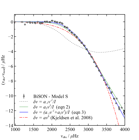
Figure 1: Frequency differences between a standard solar model (Model S, Christensen-Dalsgaard et al., 1996) and observations of low-degree modes ($\ell\leq 3$) by BiSON. The lines show fits made using an inverse term (dashed), cubic term (dotted) or both terms (solid). The fit with the inverse term is quite poor, with the cubic term much better and with both terms somewhat better still. The dot-dashed lines show a power law, fit to nine radial orders about $\nu_{\text{max}}=3090\hbox{\rm\thinspace$\mu$Hz}$, as is used in the frequency correction proposed by Kjeldsen et al. (2008).

2 Modelling and fitting of surface effects

2.1 Parametrizations

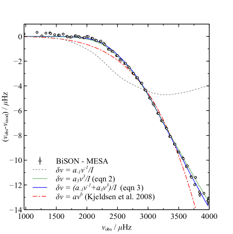
Figure 2: Frequency differences between a solar model calibrated with MESA and observations of low-degree modes ($\ell\leq 3$) by BiSON. The lines show fits made using an inverse term (dashed), cubic term (dotted) or both terms (solid). The relative performances of the fits is the same as Fig. 1. The dot-dashed lines show a power law, fit to nine radial orders about $\nu_{\text{max}}=3090\hbox{\rm\thinspace$\mu$Hz}$, as is used in the frequency correction proposed by Kjeldsen et al. (2008).

Gough (1990) discussed potential asymptotic forms for the frequency shifts observed by Libbrecht & Woodard (1990) over the solar activity cycle. By considering perturbations near the surface under a variational principle and taking the asymptotic form of the displacement eigenfunctions in the evanescent layer, Gough (1990) concluded that the frequency shifts should generally take the form (equation 9.3 of Gough, 1990)

$$\delta\nu\propto\frac{Q(\nu^{2})}{\nu\mathcal{I}}\text{,}$$ (1)

where $Q(x)$ is a quadratic function in $x$; $\nu$ is the cyclic frequency of an oscillation mode; and $\delta\nu$ is the frequency shift induced by a perturbation near the stellar surface. The normalized mode inertia $\mathcal{I}$ is defined by (e.g. Aerts et al., 2010, equation 3.140)

$$\mathcal{I}=\frac{4\pi\int_{0}^{R}\left[|\xi_{\text{r}}(r)|^{2}+\ell(\ell+1)|\xi_{\text{h}}(r)|^{2}\right]\rho r^{2}dr}{M\left[|\xi_{\text{r}}(R)|^{2}+\ell(\ell+1)|\xi_{\text{h}}(R)|^{2}\right]}\text{,}$$ (2)

where $\xi_{\text{r}}$ and $\xi_{\text{h}}$ are the radial and horizontal components of the displacement eigenvector, $R$ the photospheric radius, $\rho$ the unperturbed stellar density, $M$ the total stellar mass, and $\ell$ the degree of the mode. In the solar models, the mode inertia decreases rapidly with frequency below about $2000\hbox{\rm\thinspace$\mu$Hz}$ before levelling out and reaching a minimum around $4000\hbox{\rm\thinspace$\mu$Hz}$. This behaviour suppresses the magnitude of the frequency shifts at low frequency.

Gough (1990) further argued that a perturbation caused by a magnetic field concentrated into filaments, which would mostly modify the sound speed without much affecting the gas density, would cause a shift proportional to $\nu^{3}/\mathcal{I}$. This is the same form suggested by Goldreich et al. (1991) for photospheric perturbations. A perturbation caused by a change in the description of convection, which would presumably modify the pressure scale height, would cause a shift proportional to $\nu^{-1}/\mathcal{I}$. Following from their distinct dependences on frequency, we refer to these two terms as cubic and inverse surface effects, and to their combination as a combined surface effect.

Fig. 1 shows the difference between low-degree ($\ell\leq 3$) solar oscillation frequencies observed over 8640 days by the Birmingham Solar-Oscillations Network (BiSON, Broomhall et al., 2009) and adiabatic oscillation frequencies computed for a standard solar (Model S, Christensen-Dalsgaard et al., 1996). The curves represent uncertainty-weighted least-squares fits to the observed frequency differences using either the cubic term, the inverse term or both. The inverse term alone does not produce a good fit to the differences ($\chi^{2}=424\,092$), whereas the cubic term does ($\chi^{2}=16\,150$). The combination of both terms provides a significantly better fit ($\chi^{2}=11\,250$). Similarly, Fig. 2 shows the difference between the BiSON frequencies and a solar model computed using the solar calibration test case distributed with the Modules for Experiments in Stellar Astrophysics (MESA, Paxton et al., 2011, 2013). Again, the inverse term alone fits badly ($\chi^{2}=517\,678$), the cubic term better ($\chi^{2}=27\,287$), and their combination slightly better still ($\chi^{2}=25\,728$). The larger $\chi^{2}$ of the MESA solar model is chiefly contributed by a handful of modes below $1500\hbox{\rm\thinspace$\mu$Hz}$, where the MESA model shows systematically higher frequencies and the observed uncertainties are smallest. In fact, the two lowest-frequency modes alone contribute about $17\,000$ to $\chi^{2}$. Despite this difference, both solar models fit best with similar coefficients for the surface terms.

Figs 1 and 2 also show power-law fits as suggested by Kjeldsen et al. (2008). For each of the solar models, we fit a power law to the frequency differences for nine radial orders about $3090\hbox{\rm\thinspace$\mu$Hz}$. Though the fits are reasonably good in the fitted range, they are distinctly worse at higher and lower frequencies, as can be seen by the overprediction of the size of the correction around $2200\hbox{\rm\thinspace$\mu$Hz}$. When one considers all the modes, the power-law fits give $\chi^{2}=49\,981$ and $90\,657$ for Model S and the MESA solar model, or $46\,626$ and $75\,172$ when also fit to all the observed frequencies. The deviation is largely a result of the change of the frequency dependence of the mode inertiae around the $2500\hbox{\rm\thinspace$\mu$Hz}$. Thus, when restricted to frequencies around $3090\hbox{\rm\thinspace$\mu$Hz}$, the fit is comparably good, but its accuracy declines as the frequency range increases.

We thus propose two potential parametrizations for surface effects. Firstly, we suggest a purely cubic term,

$$\delta\nu=a_{3}(\nu/\nu_{\text{ac}})^{3}/\mathcal{I}\text{,}$$ (3)

or, secondly, a combined expression,

$$\delta\nu=\left(a_{-1}(\nu/\nu_{\text{ac}})^{-1}+a_{3}(\nu/\nu_{\text{ac}})^{3}\right)/\mathcal{I}\text{,}$$ (4)

where $a_{-1}$ and $a_{3}$ are coefficients that are to be fit for the stellar model under consideration, and $\nu_{\text{ac}}$ is the acoustic cutoff frequency, used here purely to non-dimensionalize the frequencies. For convenience, we compute $\nu_{\text{ac}}$ using the scaling relation

$$\nu_{\text{ac}}/\nu_{\text{ac},\odot}=\frac{g}{g_{\odot}}\left(\frac{T_{\text{eff}}}{T_{\text{eff},\odot}}\right)^{-1/2}$$ (5)

where we take $\nu_{\text{ac},\odot}=5000\hbox{\rm\thinspace$\mu$Hz}$.

2.2 Fitting the surface effect

This parametrization uses only global parameters of the oscillations (i.e. frequency $\nu$ and mode inertia $\mathcal{I}$), both of which are typically computed by oscillation packages (e.g. ADIPLS, Christensen-Dalsgaard, 2008). In addition, the parametrization only introduces linear terms, which can be fit analytically. It is not necessary to construct any additional stellar models or use iterative methods to compute the coefficients $a_{-1}$ and $a_{3}$, so the fit can easily be incorporated into existing model-fitting pipelines. We now describe in detail how this can be performed.

Suppose that we are comparing a stellar model, whose mode frequencies $\nu_{i,\text{mod}}$ and inertiae $\mathcal{I}_{i}$ have been computed, to a set of observed mode frequencies $\nu_{i,\text{obs}}$ with uncertainties $\sigma_{i}$. Here, $i\in\{1,\ldots,N_{\text{modes}}\}$, where $N_{\text{modes}}$ is the number of observed modes. The best-fitting coefficients for the surface effect are determined by minimizing

$$\chi^{2}_{\text{SE}}=\sum_{i=1}^{N_{\text{modes}}}\left(\frac{\nu_{i,\text{mod}}+\delta\nu_{i}-\nu_{i,\text{obs}}}{\sigma_{i}}\right)^{2}$$ (6)

with respect to the coefficients $a_{3}$ and $a_{-1}$, with $\delta\nu_{i}$ given by either of equations 3 or 4, above. Note that the coefficients are optimized with respect to all the observed frequencies rather than just the radial modes, as in the formula of Kjeldsen et al. (2008).

Because the surface effect is linear in the coefficients, the best-fitting values can be determined analytically by linear regression. Let us first define the vector $\@vec{y}$ by

$$y_{i}=\frac{\nu_{i,\text{obs}}-\nu_{i,\text{mod}}}{\sigma_{i}}\text{.}$$ (7)

For the cubic surface effect (equation 3), we further define the vector $\@vec{X}$ by

$$X_{i}=\frac{\nu_{i,\text{mod}}^{3}}{\mathcal{I}_{i}\sigma_{i}}\text{,}$$ (8)

in which case the best-fitting coefficient $a_{3}$ is

$$a_{3}=\frac{\sum_{i}{X_{i}y_{i}}}{\sum_{i}{X_{i}^{2}}}\text{.}$$ (9)

For the combined surface effect (equation 4), we instead define a matrix $\@tens{X}$ by

$$X_{i,1}=\frac{\nu_{i,\text{mod}}^{-1}}{\mathcal{I}_{i}\sigma_{i}}\text{,}\quad X_{i,2}=\frac{\nu_{i,\text{mod}}^{3}}{\mathcal{I}_{i}\sigma_{i}}\text{,}$$ (10)

in which case the best-fitting coefficients $a_{-1}$ and $a_{3}$ are given by

$$\left(\begin{array}[]{c}a_{-1}\\ a_{3}\end{array}\right)=\left(\@tens{X}^{\text{T}}\@tens{X}\right)^{-1}\@tens{X}^{\text{T}}\@vec{y}\text{.}$$ (11)

This matrix equation does not reduce to as simple a form as the cubic case but the equations are still easily solved analytically. The matrix $\@tens{X}^{\text{T}}\@tens{X}$ is only $2\times 2$-dimensional, so its inverse is trivially computed. Note that $(\@tens{X}^{\text{T}}\@tens{X})^{-1}\@tens{X}^{\text{T}}$ is simply the Moore–Penrose pseudoinverse of $\@tens{X}$.

Thus, given the mode frequencies and inertiae of a stellar model, the analytic calculation described above returns the optimal values of the coefficients in a least-squares sense. Unlike the method of Kjeldsen et al. (2008), the frequencies are not rescaled by the ratio of the modelled and observed large separation before being corrected. In their formulation, this constrains the overall scale of the frequency correction to the same as those models that have a similar large separation. Without such a rescaling, it is possible that an incorrect model could be found to fit well with unrealistically large values of the coefficients. In fact, in the new parametrization presented here, even the sign of the surface correction is currently not constrained, so there is nothing to prevent a best-fitting model that has a surface effect of opposite sign to that of the Sun. We have not found this to be a problem but we cannot demonstrate that it never will be.

A possible solution of this issue would be to penalize large values of the coefficients by choosing an appropriate prior. For example, one could assume that the logarithms of the coefficients are uniformly distributed, which is often done for parameters that represent a scale rather than a position in parameter space. This would also prevent values of opposite sign but would require modification of the analytic calculation above.

2.3 Stellar models and fitting procedure

We tested the parametrizations, using the method outline above, with the downhill simplex method (Nelder & Mead, 1965) implemented in MESA (revision 6022) optimizes the values of a stellar model’s age $t$, mass $M$, initial metallicity $[$Fe/H$]_{i}$, initial helium abundance $Y_{i}$ and mixing-length parameter $\alpha$. The combined spectroscopic constraints and corrected frequencies were used to evaluate the objective function given by

$$\chi^{2}=\sum_{i=1}^{N}\left(\frac{x_{i,\text{mod}}-x_{i,\text{obs}}}{\sigma_{i}}\right)^{2}\text{,}$$ (12)

where $x_{i,\text{obs}}$ represent all of the $N$ observations used–spectroscopic or seismic–, $\sigma_{i}$ their uncertainties, and $x_{i,\text{mod}}$ the corresponding model values. That is, we do not distinguish between any of the parameters in computing $\chi^{2}$, as in e.g. Metcalfe et al. (2014).

For comparison, we also ran the pipeline using the surface correction proposed by Kjeldsen et al. (2008), in which the surface correction is modelled as a power-law in frequency, calibrated to the Sun. By fitting the frequency differences between the BiSON data and the MESA solar model above for nine radial orders about $\nu=3090\hbox{\rm\thinspace$\mu$Hz}$, we determined the appropriate index to be $b=4.81$. This is similar to the value $b=4.9$ reported by Kjeldsen et al. (2008), which is often used without recalibration.

To compute an initial model for each evolutionary track, we first initialized a pre-main-sequence model with a central temperature $300\,000\rm\thinspace K$ and allowed it to evolve until $\log L/\hbox{$\rm\thinspace L_{\sun}$}=0.4$, where $L$ and $\rm\thinspace L_{\sun}$ are the total stellar and solar luminosities. At the beginning of each track, this model was then rescaled by mass to the value being evaluated, from its existing mass of $1\hbox{$\rm\thinspace M_{\sun}$}$ for the synthetic and degraded solar fits, and $1.2\hbox{$\rm\thinspace M_{\sun}$}$ for HD 52265. In both cases, these models had ages less than $2\rm\thinspace Myr$. Stellar models were evolved starting from the pre-main-sequence model described above until a minimum of $\chi^{2}$ had been found and one of the spectroscopic constraints was beyond its observed value by $5\sigma$. The parameters of the stellar model (including the age of the optimal fit along that track) are then used to update the simplex.

For the constitutive physics, we use opacities from the OPAL tables (Iglesias & Rogers, 1996) and Ferguson et al. (2005) at high and low temperatures, respectively, blended linearly in the range $4.00\leq\log T\leq 4.10$. A standard Eddington grey atmosphere is employed and convective processes are described by mixing-length theory according to Henyey et al. (1965). In the synthetic and Sun-as-a-star fits, convective overshooting was fixed at its solar-calibrated value. For HD 52265, no overshooting was included. The composition was scaled from the solar values given by Grevesse & Sauval (1998). Diffusion and gravitational settling are included through the method of Thoul et al. (1994). Nuclear reaction rates are drawn from Caughlan & Fowler (1988) or the NACRE collaboration (Angulo et al., 1999), with preference given to the latter when available. We used newer specific reaction rates for the reactions ${}^{14}\mathrm{N}(p,\gamma){}^{15}\mathrm{O}$ (Imbriani et al., 2005) and ${}^{12}\mathrm{C}(\alpha,\gamma){}^{16}\mathrm{O}$ (Kunz et al., 2002). All other options took default values, which are described in the MESA instrument papers (Paxton et al., 2011, 2013) and available in the source code.

The oscillation frequencies and mode inertiae were computed using the Aarhus adiabatic oscillation package (ADIPLS, Christensen-Dalsgaard, 2008), without remeshing the stellar model. The models were computed with a mesh-spacing coefficient $C=1/2$, which corresponds to about 1500 meshpoints. This is sufficient to correctly compute oscillation frequencies and mode inertiae along the main sequence. Calls to ADIPLS are made from MESA during the stellar evolution calculation and by default return the frequencies and inertiae.

We set the parameter tolerance in the downhill simplex method to $10^{-5}$. For the synthetic data, the initial parameters used the same parameters as for the input model. For the Sun, the initial parameters were the calibrated values given by Paxton et al. (2013). Finally, for HD 52265, we began with parameters computed by a fit to the spectroscopic parameters and averaged large and small separations, as measured by Ballot et al. (2011), and then found best-fit model parameters for the unperturbed observations with a cubic surface effect. These parameters were used as the initial guess for all the fits to HD 52265.

We then used the observed uncertainties to generate 100 random realizations of the observations and fit a stellar model to each realization, using the parameters of the primary model as the initial guess. The reported values are the $15.85$, $50$ and $84.15$ percentiles for the relevant distributions. i.e. the median and a $68.3$ per cent confidence interval for the sample of 100 fits.

Because different choices of timestep can lead to slightly different models for a given set of parameters, the timesteps were fixed at $10\rm\thinspace Myr$ when fitting the synthetic data, the same value used to compute the input model. For the fits to the degraded BiSON observations and HD 52265, the timestep was decreased adaptively from $30\rm\thinspace Myr$ to $300\,000\rm\thinspace yr$ based on partial evaluations of $\chi^{2}$ dropping below certain limits.

The results of all of the fits are presented in Table 1.

Table 1: Results of all fits presented here, as well as fits for HD 52265 presented by Escobar et al. (2012) and spectroscopic inputs for all fits (labelled Input). The central values are the medians and the upper and lower limits are the locations of the $15.85$ and $85.15$ percentiles. In the case of the synthetic data, we also include the parameter values used to generate the observations.

Synthetic	$t/\text{Gyr}$	$M/\hbox{$\rm\thinspace M_{\sun}$}$	$[$Fe/H$]_{i}$	$Y_{i}$	$\alpha$	$a_{3}/10^{-7}\hbox{\rm\thinspace$\mu$Hz}$	$a_{-1}/10^{-9}\hbox{\rm\thinspace$\mu$Hz}$	$T_{\text{eff}}/\text{K}$	$\log g$	$\log L/\hbox{$\rm\thinspace L_{\sun}$}$	$[$Fe/H$]_{s}$	$R/\hbox{$\rm\thinspace R_{\sun}$}$
Input	$4.61$	$1.000$	$0.097$	$0.2784$	$1.908$			$5773\pm 60$	$4.45\pm 0.09$	$-0.01\pm 0.05$	$0.04\pm 0.05$	$0.9918$
A	$4.64^{+0.23}_{-0.27}$	$0.999^{+0.002}_{-0.005}$	$0.098^{+0.011}_{-0.014}$	$0.2780^{+0.0006}_{-0.0004}$	$1.90^{+0.03}_{-0.05}$	$0.00^{+0.06}_{-0.10}$		$5766^{+43}_{-41}$	$4.4451^{+0.0006}_{-0.0008}$	$-0.010^{+0.012}_{-0.014}$	$0.040^{+0.012}_{-0.014}$	$0.9911^{+0.0006}_{-0.0016}$
B	$4.58^{+0.26}_{-0.21}$	$0.999^{+0.002}_{-0.005}$	$0.096^{+0.014}_{-0.020}$	$0.2781^{+0.0005}_{-0.0004}$	$1.91^{+0.03}_{-0.06}$	$-1.90^{+0.10}_{-0.08}$		$5769^{+46}_{-54}$	$4.4452^{+0.0004}_{-0.0009}$	$-0.010^{+0.014}_{-0.017}$	$0.038^{+0.014}_{-0.020}$	$0.9911^{+0.0006}_{-0.0014}$
C	$4.64^{+0.28}_{-0.25}$	$0.999^{+0.012}_{-0.009}$	$0.093^{+0.037}_{-0.019}$	$0.2778^{+0.0009}_{-0.0011}$	$1.91^{+0.08}_{-0.09}$	$-0.01^{+0.23}_{-0.20}$	$0.71^{+6.90}_{-7.88}$	$5772^{+70}_{-78}$	$4.4451^{+0.0016}_{-0.0015}$	$-0.009^{+0.023}_{-0.026}$	$0.035^{+0.039}_{-0.019}$	$0.9911^{+0.0041}_{-0.0032}$
D	$4.62^{+0.31}_{-0.23}$	$1.000^{+0.015}_{-0.011}$	$0.093^{+0.037}_{-0.033}$	$0.2778^{+0.0011}_{-0.0015}$	$1.91^{+0.11}_{-0.07}$	$-2.05^{+0.32}_{-0.24}$	$4.22^{+6.77}_{-6.37}$	$5768^{+78}_{-52}$	$4.4453^{+0.0017}_{-0.0019}$	$-0.011^{+0.029}_{-0.018}$	$0.034^{+0.040}_{-0.035}$	$0.9913^{+0.0053}_{-0.0035}$
Sun-as-a-star
Input								$5778\pm 60$	$4.44\pm 0.09$	$0.000\pm 0.024$	$0.00\pm 0.05$
E	$4.74^{+0.18}_{-0.19}$	$1.000^{+0.015}_{-0.010}$	$0.083^{+0.020}_{-0.045}$	$0.276^{+0.006}_{-0.018}$	$1.83^{+0.05}_{-0.07}$	$-2.47^{+0.14}_{-0.44}$		$5768^{+48}_{-46}$	$4.4382^{+0.0020}_{-0.0013}$	$-0.001^{+0.014}_{-0.017}$	$0.023^{+0.022}_{-0.047}$	$1.000^{+0.005}_{-0.003}$
F	$4.68^{+0.30}_{-0.19}$	$1.000^{+0.014}_{-0.007}$	$0.085^{+0.017}_{-0.043}$	$0.278^{+0.006}_{-0.017}$	$1.84^{+0.04}_{-0.05}$	$-2.45^{+0.15}_{-0.26}$	$2.34^{+7.62}_{-7.61}$	$5779^{+38}_{-43}$	$4.4383^{+0.0020}_{-0.0013}$	$0.002^{+0.012}_{-0.014}$	$0.026^{+0.017}_{-0.047}$	$1.000^{+0.004}_{-0.003}$
G	$4.75^{+0.25}_{-0.32}$	$1.003^{+0.010}_{-0.007}$	$0.091^{+0.012}_{-0.012}$	$0.277^{+0.005}_{-0.011}$	$1.87^{+0.04}_{-0.05}$			$5786^{+58}_{-50}$	$4.4381^{+0.0015}_{-0.0009}$	$0.007^{+0.014}_{-0.014}$	$0.033^{+0.013}_{-0.012}$	$1.001^{+0.003}_{-0.002}$
HD 52265
Input								$6100\pm 60$	$4.35\pm 0.09$	$0.328\pm 0.024$	$0.19\pm 0.05$
H	$2.44^{+0.16}_{-0.15}$	$1.215^{+0.030}_{-0.008}$	$0.259^{+0.030}_{-0.040}$	$0.292^{+0.006}_{-0.029}$	$1.64^{+0.07}_{-0.06}$	$-3.40^{+0.49}_{-0.51}$		$6056^{+40}_{-40}$	$4.2853^{+0.0052}_{-0.0012}$	$0.322^{+0.015}_{-0.013}$	$0.161^{+0.034}_{-0.042}$	$1.314^{+0.008}_{-0.002}$
I	$2.44^{+0.13}_{-0.09}$	$1.211^{+0.007}_{-0.007}$	$0.264^{+0.029}_{-0.026}$	$0.294^{+0.005}_{-0.004}$	$1.63^{+0.07}_{-0.04}$	$-3.41^{+0.39}_{-0.36}$	$11.19^{+7.39}_{-5.77}$	$6057^{+55}_{-38}$	$4.2842^{+0.0009}_{-0.0013}$	$0.320^{+0.014}_{-0.010}$	$0.164^{+0.033}_{-0.029}$	$1.313^{+0.004}_{-0.003}$
J	$2.26^{+0.18}_{-0.11}$	$1.222^{+0.020}_{-0.005}$	$0.312^{+0.024}_{-0.035}$	$0.301^{+0.006}_{-0.009}$	$1.66^{+0.08}_{-0.06}$			$6073^{+56}_{-58}$	$4.2854^{+0.0016}_{-0.0010}$	$0.329^{+0.018}_{-0.012}$	$0.218^{+0.030}_{-0.039}$	$1.319^{+0.008}_{-0.003}$
TGEC	$2.6\pm 0.2$	$1.24\pm 0.02$	$0.27\pm 0.04$	$0.28\pm 0.02$				$6120\pm 20$	$4.284\pm 0.002$	$0.348\pm 0.006$	$0.20\pm 0.04$	$1.33\pm 0.02$
AMP(a)	$3.00$	$1.22$	$0.23$	$0.280$				6019	4.282	0.313		1.321
AMP(b)	$2.38$	$1.20$	$0.215$	$0.298$				6097	4.282	0.328		1.310

3 Tests on synthetic and solar data

3.1 Synthetic data

We first tested whether our method correctly recovers synthetic input data. We constructed a stellar model with input parameters taken from the solar calibration presented by Paxton et al. (2013) and computed its oscillation frequencies and mode inertiae. We then used its observable properties as inputs for our modelling pipeline, using the same selection of observables as is available for HD 52265, along with the corresponding uncertainties. The spectroscopic parameters are the effective temperature $T_{\text{eff}}$, surface gravity $\log g$, metallicity $[$Fe/H$]_{s}$ and luminosity $\log L/\hbox{$\rm\thinspace L_{\sun}$}$. We fit the frequencies of 28 oscillation modes: 10 radial, 10 dipole, and 8 quadrupole modes, centred on $\nu_{\text{max}}\approx 3000$. These observable constraints are fairly typical for a star with good spectroscopic and intermediate seismic observations, with a timeseries of 117 days.

We first tested the cubic-only surface effect, first by fitting the synthetic data without any surface effect (case A) and second by fitting with a surface effect with $a_{3}=-1.87\times 10^{-7}\hbox{\rm\thinspace$\mu$Hz}$ (case B). We then tested the combined surface effect, again first without a surface effect (case C) and then with an artificial surface effect (case D) with $a_{-1}=2.07\times 10^{-7}\hbox{\rm\thinspace$\mu$Hz}$ and $a_{3}=-2.78\times 10^{-9}\hbox{\rm\thinspace$\mu$Hz}$. The results are labelled correspondingly in Table 1.

In all four cases, the fitted parameters are consistent with the input parameters, be it with or without a surface effect, cubic or combined. We also confirmed that the parameters of the input model give a perfect fit. i.e. $\chi^{2}=0$, as expected.

In cases C and D, $a_{-1}$ is consistent with the input value but comes with large uncertainties. In fact, in case D, the result is consistent with $a_{-1}=0$. This is unsurprising, given that the range of observed frequencies does not extend to the bend in the surface effect caused by the sharp frequency dependence of the mode inertiae at low frequencies. In addition, Figs 1 and 2 show that the surface effect is dominated by the cubic term, especially at frequencies about about $2500\hbox{\rm\thinspace$\mu$Hz}$.

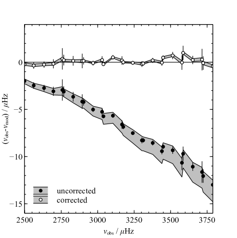
Figure 3: Uncorrected and corrected frequency differences between observed frequencies for the degraded solar data and MESA models fit using only the cubic term (equation 3). The solid and empty points show the uncorrected and corrected differences with error bars that correspond to the observed uncertainties. The shaded regions show the spread of the modelled frequencies. i.e. taken from the 100 fits to random realizations of the observations. There is no obvious remaining trend in the corrected frequencies.

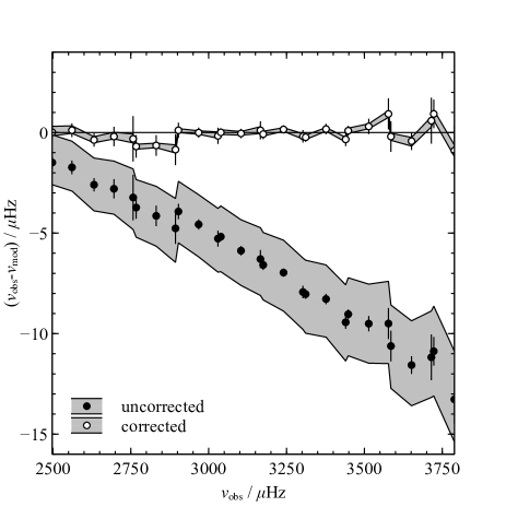
Figure 4: As in Fig. 3 but with a fit made using the combined surface term (equation 4).

Figure 5: As in Fig. 3 but with a fit made using the rescaled power law proposed by Kjeldsen et al. (2008). Note that, as seen for the fits to the solar data in Figs 1 and 2, the correction is slightly overestimated at low frequencies.

3.2 Solar data

As a second test, we perform a Sun-as-a-star experiment, where we degrade observations of the Sun to the same selection and uncertainties as observations of HD 52265. We fit the observations with the cubic term (case E), the combined terms (case F), or the scaled power law (case G), the results of which are presented in Table 1.

The fitted parameters are all consistent with our knowledge of the Sun, although the mixing length parameter $\alpha$ is consistently somewhat lower than the calibrated value of $1.908$. The oscillation frequencies tightly constrain the mechanical structure of the star and thus the mass, radius and combinations thereof, like mean density and surface gravity. As noted when fitting the synthetic data, the inverse term is not well-constrained, but its inclusion does not appear to greatly worsen the quality of the fit. The surface terms themselves are consistent with the coefficients determined by fitting the BiSON frequencies to the calibrated solar model (see Fig. 2): $a_{3}=-2.13\times 10^{-7}\hbox{\rm\thinspace$\mu$Hz}$ for the cubic fit, and $a_{3}=-2.25\times 10^{-7}\hbox{\rm\thinspace$\mu$Hz}$ and $a_{-1}=1.73\times 10^{-9}\hbox{\rm\thinspace$\mu$Hz}$ for the combined fit.

The frequency differences for cases E, F, and G are shown in Figs 3, 4, and 5. The error bars on the data points represent the observed uncertainties; the shaded regions around the corrected and uncorrected differences represent the spread in the 100 fits to independent realizations. The quality of the new fits to the corrected frequencies is encouraging, given that there are no obvious remaining trends in either case. The power-law fit shows a marginal trend in the residual differences, with the corrected model frequencies being too high at low frequencies. This is consistent with the fits to solar data in Figs 1 and 2.

It is clear from Figs 3 and 4 that simultaneously fitting the surface effect with the cubic or combined terms allows a greater range of models than the observed uncertainties. This can be seen in the fact that the envelope of model uncertainties is broader for the uncorrected than the corrected frequencies. In essence, the uncertainty about the surface effects is reflected in the uncertainties of the underlying stellar parameters but every model is optimally corrected to match the observed frequencies. For example, consider case E, where only the cubic term was used. The uncertainty in the coefficient $a_{3}$ is about 10 per cent, which naively permits an uncertainty of about $1\hbox{\rm\thinspace$\mu$Hz}$ for a $10\hbox{\rm\thinspace$\mu$Hz}$ frequency shift, all else being equal. In reality, the coefficients are correlated with the underlying model parameters, so this estimate is only approximate. When using both terms, an even greater range of models is allowed and the uncertainties are correspondingly larger.

In addition, the uncertainties of the corrected model frequencies are generally smaller than the observed uncertainties. This follows from the random realization process. In the observations, the uncertainties are uncorrelated, so the observed frequencies are perturbed independently. In the stellar models, the variations of the frequencies with respect to the stellar parameters are instead tightly correlated. It is highly unlikely that a random realization of the observations reproduces the correlated variations of the model frequencies, so the underlying parameters vary relatively little from their best-fitting values.

4 Application to HD 52265

HD 52265 is a metal-rich G0V planet-hosting star that was observed by CoRoT for 117 days between November 2008 and March 2009. Ballot et al. (2011) reported spectroscopic and seismic observations that Escobar et al. (2012) used to perform a detailed analysis of the star. This involved the direct comparison of manually-selected models (TGEC) and two automated fits using the Asteroseismic Modelling Portal (AMP, Metcalfe et al., 2009): one using all the frequencies given by Ballot et al. (2011) (fit (a)) and one omitting the lowest three frequencies, as is done here (fit (b)). Lebreton & Goupil (2012) estimated the extent of inward convective overshooting using stellar models with $t\approx 2\rm\thinspace Gyr$, $M\approx 1.25\hbox{$\rm\thinspace M_{\sun}$}$, and $R\approx 1.3\hbox{$\rm\thinspace R_{\sun}$}$, in reasonable agreement with the results presented here, although they do not report quantitative uncertainties on the model parameters. They do estimate the depth of the convective zone, with penetrative overshooting, to be $R_{\text{cz}}=0.800\pm 0.004\,R_{*}$, where $R_{*}$ is the radius of the star. This is compatible with our result of $R_{\text{cz}}/R_{*}=0.803$ for the best-fitting stellar model. Finally, HD 52265 was modelled using the SEEK pipeline (Quirion et al., 2010), as reported in Escobar et al. (2012) and Gizon et al. (2013), which returned best-fit parameters $t=2.37\pm 0.29\rm\thinspace Gyr$, $M=1.27\pm 0.03\hbox{$\rm\thinspace M_{\sun}$}$, and $R=1.34\pm 0.02\hbox{$\rm\thinspace R_{\sun}$}$. The higher mass is somewhat discrepant, and Escobar et al. (2012) argued that it represents a local, secondary, optimum of the model parameters. The spectroscopic observations are listed in Table 1, along with model parameters for the TGEC and AMP fits by Escobar et al. (2012), and the results presented in this paper. For the frequency selection, we used the reported frequencies for 10 $\ell=0$, 10 $\ell=1$ and 8 $\ell=2$ oscillation modes between $1600$ and $2550\hbox{\rm\thinspace$\mu$Hz}$. We omitted the lowest three frequencies given by Ballot et al. (2011), which are reportedly less reliable.

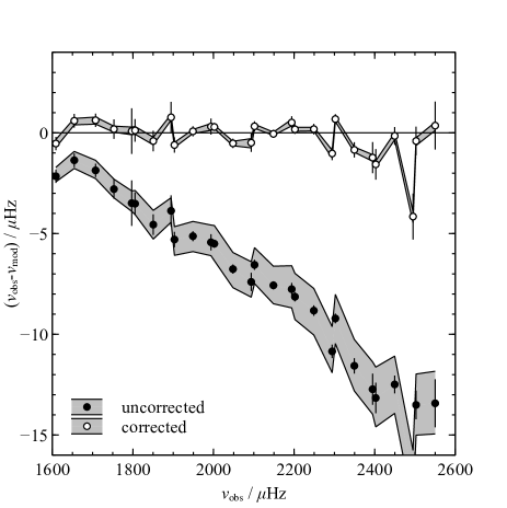
Figure 6: As in Fig. 3 for the fit to HD 52265 using the cubic term (equation 3).

The fits with the cubic, combined, and power-law surface terms (cases H, I, and J) are included in Table 1. We have also included the best-fit parameters reported by Escobar et al. (2012) for comparison, and our results with the cubic and combined surface terms are entirely consistent. Like previous models, we find that the surface gravity is lower (though not significantly) than the spectroscopic value. In addition, the parameter fits made with the combined surface term are consistent with those made with the cubic term only.

Figs 6, 7, and 8 show the frequency differences for the cubic, combined, and power-law surface terms. For the cubic and combined terms, there is again no obvious residual, though the highest-frequency $\ell=2$ mode shows a significant remaining difference. In both cases, the overall scale of the surface effect is similar to that of the Sun, taking a value of roughly $7\hbox{\rm\thinspace$\mu$Hz}$ at $\nu_{\text{max}}\approx 2100\hbox{\rm\thinspace$\mu$Hz}$. The coefficients of the cubic term also of similar size, when the oscillation frequencies are normalized against the acoustic cutoff frequency. The coefficient of the inverse term is non-zero at the $2\sigma$ level, although still consistent with the Sun-as-a-star value because of the large uncertainties. As noted before, the addition of the inverse term does not appear to improve the fit significantly, although it similarly does no harm. This is also presumably due to the limited number of radial orders covered by our frequency selection.

The power-law fit again shows a slight residual trend but the overall correction is similar. However, the quality of the fit is significantly worse than the cubic term. The differences between the corrected and observed frequencies for the best-fitting models give $\chi^{2}=124$ for the scaled power-law compared with $\chi^{2}=31$ for the cubic term. The underlying model parameters deviate only within uncertainties but we expect that they would deviate further as the number of observed modes increases and the shape of the surface effect deviates from a power law. Thus, given the smaller values of $\chi^{2}$ in both HD 52265 and the full set of BiSON frequencies, we believe that the cubic term produces better best-fit parameters than the scaled power law.

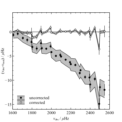
Figure 7: As in Fig. 3 for the fit to HD 52265 using the combined term (equation 4).

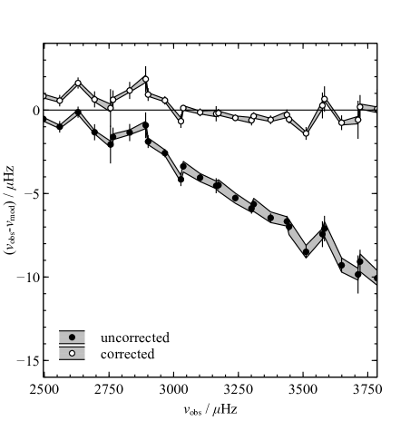
Figure 8: As in Fig. 3 but for a fit to HD 52265 made using the rescaled power law proposed by Kjeldsen et al. (2008). Again, the correction is slightly overestimated at low frequencies.

5 Discussion

5.1 Quality of parametrization fits

Based on the results presented here, it appears that the proposed parametrizations of the surface effects can adequately describe the true surface effects, certainly enough to correctly recover the underlying stellar model parameters. In all cases, the price to pay is increased uncertainties in the uncorrected frequencies, even though the corrected frequencies have small uncertainties. Despite this loss of accuracy, the exploitation of the full set of frequencies, even given a relatively meagre selection of mode frequencies, allows precise determination of the underlying stellar model parameters.

For the degraded BiSON data, the scaled power-law correction gives consistent results. In this case the index of the power law has been fit directly to the star in question, and the fit is about as good as the new parameterizations over the observed range. There is, however, an uncorrected trend, which would induce greater discrepancies in the stellar model parameters given a larger frequency range. In the case of HD 52265, the fit is significantly worse, although the stellar parameters continue to be consistent. The poor fit is not because a power law describes the frequency differences badly, but rather because the solar-calibrated value of the index is incorrect. For comparison, if we fit a power law to the frequency differences of the best fit model with the cubic term, we find $b=4.11$, which is smaller than the solar-calibrated value of $b=4.81$. The use of the mode inertia appears to capture the variation of the power law between the two stars studied here.

In the Sun, the surface effect appears to be dominated by the cubic term and the frequency range used here does not strongly constrain the inverse term. We recommend that stellar models are first fit using only the cubic term and that the inverse term be introduced as an additional parameter after the initial fit has been performed. A greater number of lower-order frequencies would better constrain the inverse term to determine whether its contribution remains small. In fact, generally speaking, lower order modes constrain any surface term better, because those modes are affected least. Such observations are most easily made when frequencies are determined from radial velocity data rather than photometric data. The proposed Stellar Observations Network Group (SONG, Grundahl et al., 2014), of which one node is now essentially operational, would be invaluable in making such observations.

5.2 Uncertainties

Our uncertainties for the parameters of HD 52265 are generally smaller than those reported by Escobar et al. (2012) for the TGEC models. Their model parameters were derived from the mean and standard deviation of three manually chosen best-fitting models. The results from the AMP are reported without uncertainties. Thus, our smaller uncertainties are not necessarily at odds with the TGEC fit. The uncertainty on the initial helium abundance $Y_{i}$ may seem particularly small, but it is consistent with the uncertainty on the initial metallicity. If we suppose that the initial helium and metal abundances are related by some enrichment law$Y=Y_{0}+(\Delta Y/\Delta Z)Z$ and that

$$[{\rm Fe/H}]=\log(Z/X)-\log(Z/X)_{\odot}\text{,}$$ (13)

with some primordial helium abundance $Y_{0}$, then it is possible to solve for the $Y$ given $[$Fe/H$]$. By taking, for example, $Y_{0}=0.245$ and $\Delta Y/\Delta Z=1.4$, then a change in $[$Fe/H$]_{i}$ from $0.27$ to $0.30$ induces a change of just $0.002$ in $Y_{i}$. Thus, the uncertainties, though small, are compatible with our knowledge of the initial metallicity, even though the helium and metal abundance were fit independently.

The uncertainties of the fits to the synthetic data are smaller still because the central values, about which the random realizations are made, are perfectly consistent. Similarly, central values of the degraded solar data are based on the BiSON data, for which the uncertainties are also very small. Thus, even though we have used greater uncertainties to randomly realize observations, the parameter space is dominated by a deeper optimal solution.

We also note that the uncertainties reported here are purely statistical. They do not reflect uncertainties in the input model physics that would be induced by changing, for example, the opacity tables, equation of state, or atmospheric model. This is an interesting problem that has not yet been extensively studied for fits using individual frequencies. Chaplin et al. (2014) analyzed several hundred Kepler short-cadence targets using six stellar evolution codes across 11 pipelines and concluded that the uncertainties induced by different codes and pipelines are about 3.7, 1.7, and 16 per cent in mass, radius, and age, when spectroscopic constraints on $T_{\text{eff}}$, $\log g$ and $[$Fe/H$]$ are available. These fits were not based on individually-resolved frequencies, which presumably constrain models better than overall seismic properties, but they still inform us on the differences caused by using different stellar models. In the future, we intend to study the systematic errors in detail by exploiting the modular design of MESA to isolate the effects of individual choices of input physics.

5.3 Potential shortcomings

Despite performing well on the targets studied here, the method does contain several potential flaws. First, as is always the case with optimization problems, we cannot guarantee that we have found the global best-fit solution. To some extent, the repeated random realizations mitigate this problem because if a much better minimum were available, we might expect at least a few of the random realizations to converge there. Indeed, this is the case in HD 52265 where, in cases H and I, about 15 and 3 models settled on a secondary minimum with a mass of roughly $1.30\hbox{$\rm\thinspace M_{\sun}$}$, close to the value identified by Escobar et al. (2012). The asymmetry of the uncertainties in Table 1 captures the existence of this alternative local optimum. An initial grid-based search could also rule out the existence of better minima in distinctly different regions of parameter space. The greater problem is that the introduction of one or two new free parameters, which are simultaneously optimized during the fit and currently not limited in scale or sign, might introduce new local minima that confuse the optimization process. We propose to mitigate this by choosing initial guesses that weight non-seismic observations more heavily, though the final sample of fits should continue to be performed without artificially weighting the observables.

Second, there is an additional implicit free parameter: the depth of the normalization of the mode inertiae, which controls the depth of the perturbation that produces the surface effect. Here, we have used the radius of the photosphere. This is a reasonable choice and fits the Sun well but there is no guarantee that this will be the case for stars significantly different from the Sun. Rosenthal et al. (1999) computed the frequency differences between a solar model and a detailed simulation of the Sun’s surface convection zone and found that the surface effect is largely (but not entirely) produced by the suspension of the envelope by turbulent pressure, which peaks in a narrow region that is essentially at the photosphere. Recent simulations (e.g. Beeck et al., 2013; Magic et al., 2013; Trampedach et al., 2013) should allow similar studies to be carried out for a range of stellar surface properties and allow some forward computation of the expected location and scale of the surface correction. Presently, it seems reasonable to continue to normalize the mode inertiae at the photosphere.

Third, our assessment of the parametrizations is specific to the traditional mixing-length theory and adiabatic pulsations. Though not widely implemented, other one-dimensional descriptions of convection exist (e.g. full spectrum turbulence, Canuto & Mazzitelli, 1991) and these predict different properties for the superadiabatic layers near the surfaces of Sun-like stars. Since this region introduces some component of the surface effect, the parametrizations presented here may no longer fit so well. Similarly, non-adiabatic pulsation frequencies exhibit a kind of surface effect, which also may or may not be described precisely by the parametrizations.

6 Conclusion

We have presented two parametrizations of the known systematic difference between modelled and observed stellar oscillation frequencies induced by poor-modelling of the near-surface layers. The first contains a term proportional to $\nu^{3}/\mathcal{I}$ (the cubic term, equation 3) and the second an additional term proportional to $\nu^{-1}/\mathcal{I}$ (the inverse term, equation 4). The second parametrization corrects most of the frequency differences between two calibrated solar models and observed solar oscillation frequencies, in the sense that no obvious trends remain. Both parametrizations fit the frequency differences significantly better than power laws.

We implemented a simultaneous fit to the surface effects in MESA and constructed a model-fitting pipeline that fits stellar models to 100 random realizations of the observable data. By testing the new pipeline on data for a synthetic target, the Sun, and the CoRoT target HD 52265, we have shown that these parametrizations give unbiased results that are compatible with independent measurements and model fits. We compared our results with calculations made with the same pipeline, but using the scaled power-law proposed by Kjeldsen et al. (2008). In the case of the Sun, both methods perform similarly well, but for HD 52265, the power-law fit produces a significantly worse fit to the frequencies but consistent stellar parameters. Thus, the cubic term alone is arguably an improvement over a scaled power law.

Generally, the cubic term dominates the surface correction. The contribution of the inverse term is clear when comparing observations to calibrated solar models, but poorly-constrained by the small range of radial orders that we have used in the fitting pipeline. In all cases, the stellar model parameters are consistent, irrelevant of which surface term is used, and the overall scale of the surface term is similar in the Sun and HD 52265.

The simultaneous fit potentially introduces new local minima to the models’ parameter space and we recommend that initial guesses be found by weighting complementary non-seismic observations more strongly. Given a reasonable initial guess, however, we have found that the pipeline converges on a reasonable solution even though the magnitudes and signs of the coefficients are not constrained. In upcoming work, we will apply our pipeline to more stars, covering a greater range of parameters, to ensure that the parametrizations are generally useful in allowing us to exploit present and future observations of resolved oscillation modes.