Bayesian estimation of realized stochastic volatility model by Hybrid Monte Carlo algorithm

Abstract

The hybrid Monte Carlo algorithm (HMCA) is applied for Bayesian parameter estimation of the realized stochastic volatility (RSV) model. Using the 2nd order minimum norm integrator (2MNI) for the molecular dynamics (MD) simulation in the HMCA, we find that the 2MNI is more efficient than the conventional leapfrog integrator. We also find that the autocorrelation time of the volatility variables sampled by the HMCA is very short. Thus it is concluded that the HMCA with the 2MNI is an efficient algorithm for parameter estimations of the RSV model.

1 Introduction

In empirical finance, volatility of asset returns plays an important role to manage financial risk. Since volatility is not directly observed in financial markets, one needs to estimate volatility from observed quantities in the markets. A typical way to estimate volatility is to use parametric models which mimic properties of asset returns. One of such models is the stochastic volatility (SV) model[1] which allows the volatility to be a stochastic process. Recently an SV-type model that further utilizes daily realized volatilities (RV) [2, 3] was proposed[4]. This model is called the RSV model. An advantage of the RSV model is that it uses the RV as additional information to the model and thus can estimate the daily volatility more accurately.

To estimate parameters of SV-type models one usually use the Markov Chain Monte Carlo (MCMC) method based on the Bayesian approach[5, 6, 7]. In the MCMC method of the SV model the most time-consuming part is the volatility update. The number of the volatility variables to be updated increases with the data size of time series. Generally a local update algorithm such as the Metropolis algorithm is not efficient for the update of volatility variables.

In this study we use an alternative MCMC method, the HMCA[8] to estimate the parameters of the RSV model. The main advantage of the HMCA is that it is a global update algorithm that can update volatility variables simultaneously. The HMCA has been tested for the SV model[9, 10, 11] and it is found that the HMCA can de-correlate MCMC samples of volatility variables faster than the Metropolis algorithm. In this study we investigate the performance of the HMCA for the RSV model. We also examine the efficiency of an improved integrator called the 2nd order minimum norm integrator (2MNI) used for the MD simulation in the HMCA.

2 Realized Stochastic Volatility Model

The basic realized stochastic volatility (RSV) model by Takahashi et al.[4] is given by

$$y_{t} = \exp(h_{t}/2)\epsilon_{t},\hskip 14.22636pt\epsilon_{t}\sim N(0,1),$$ (1)

$$\ln RV_{t} = \xi+h_{t}+u_{t},\hskip 14.22636ptu_{t}\sim N(0,\sigma_{u}^{2}),$$ (2)

$$h_{t+1} = \mu+\phi(h_{t}-\mu)+\eta_{t},\hskip 14.22636pt\eta_{t}\sim N(0,\sigma_{\eta}^{2}),$$ (3)

where $y_{t}$ and $RV_{t}$ are a daily return and a daily realized volatility at time $t$ respectively, and $h_{t}$ is a latent volatility defined by $\ln\sigma_{t}^{2}$. This model contains 5 parameters (${\bf\theta}=\phi,\mu,\xi,\sigma_{\eta}^{2},\sigma_{u}^{2}$) that have to be determined so that the model matches the underlying returns and realized volatilities. We apply the Bayesian inference for parameter estimations and perform the Bayesian inference by the MCMC method. For the MCMC simulation of volatility variables we use the HMCA. On the other hand, we update model parameters by the standard MCMC method previously used in parameter estimations of the SV model[5, 6, 7, 9].

3 Hybrid Monte Carlo Algorithm

Originally the HMCA was invented and developed for the MCMC simulations of the lattice Quantum Chromo Dynamics (QCD) calculations[8] where non-linear interactions between gauge variables are major obstacles to perform the MCMC method[14]. The basic idea of the HMCA is a combination of the MD simulation and the Metropolis accept/reject test. Candidates for next volatility variables in Markov chain are obtained by solving the Hamilton’s equations of motion (HEOM) in fictitious time $\tau$, $\displaystyle\frac{dh_{i}}{d\tau}=\frac{\partial H}{\partial p_{i}},\hskip 5.69054pt\frac{dp_{i}}{d\tau}=-\frac{\partial H}{\partial h_{i}},$ where $p_{i}$ is a conjugate momentum to $h_{i}$. The Hamiltonian $H$ is defined by $H(p,h)=\frac{1}{2}\sum_{i}^{n}p_{i}^{2}-\ln f(h,\theta)$, where $f(h,\theta)$ is the conditional posterior density of the RSV model[4]. Since in general HEOM can not be solved analytically, we integrate them numerically through the MD simulation. The conventional integrator for the MD simulation in the HMCA is the 2nd order leapfrog integrator (2LFI)[8] given by

$$h_{i}(\tau+\delta\tau/2)=h_{i}(\tau)+\frac{\delta\tau}{2}p_{i}(\tau),\hskip 14.22636ptp_{i}(\tau+\delta\tau)=p_{i}(\tau)-\delta\tau\frac{\partial H}{\partial h_{i}},$$ (4)

$$h_{i}(\tau+\delta\tau)=h_{i}(\tau+\delta\tau/2)+\frac{\delta\tau}{2}p_{i}(\tau+\delta\tau),$$

where $\delta\tau$ stands for the step size in the MD simulation. In the operator representation the 2LFI can be expressed as $\displaystyle e^{\lambda\delta\tau T/2}e^{\delta\tau V}e^{\lambda\delta\tau T/2}$, where $T$ and $V$ are the linear operators corresponding to the kinetic term and potential term of the Hamiltonian respectively[15, 16] Eqs.(3) are repeatedly applied and, volatility and momentum variables are integrated up to a certain time $l$ called the total integration length. The numerical integration introduces the integration errors that violate the conservation of the Hamiltonian. Let $h^{\prime}$ and $p^{\prime}$ be volatilities and momenta after integration. Then we define the difference of the Hamiltonian between after and before integration as $\Delta H=H(p^{\prime},h^{\prime})-H(p,h)$. Finally new candidates for volatilities $h_{t}^{\prime}$ are accepted according to the Metropolis probability, $\min\{1,\exp(-\Delta H)\}$.

The magnitude of $\Delta H$ depends on the integrator we choose. It is possible to use higher order integrators (HOI) that can decrease the magnitude of $\Delta H$ at the same step size and increase the Metropolis acceptance. On the other hand HOI are usually computationally expensive. Therefore the total performance of HOI is not known a priori and depends on the model we use[9, 10]. In Ref.[11] it is shown that an improved integrator called the 2MNIet al.[12] is superior to the 2LFI for the lattice QCD simulations. The 2MNI is expressed as $\displaystyle e^{\lambda\delta\tau T}e^{\delta\tau V/2}e^{(1-2\lambda)\delta\tau T}e^{\delta\tau V/2}e^{\lambda\delta\tau T}$ where $\lambda$ is a tunable parameter. $\lambda$ is set to 0.193183327. This value is approximately the optimum value that minimizes the error function of 2MNI[12]. In this study we also use the 2MNI for the HMCA and examine its efficiency for the HMCA of the RSV model.

4 Simulation Study

We generated artificially 4000 data with RSV parameters $(\phi,\mu,\xi,\sigma_{\eta}^{2},\sigma_{u}^{2})=(0.93,-1.0,0.3,0.1,0.2)$ and performed the Bayesian estimation of the RSV model for this artificial data.

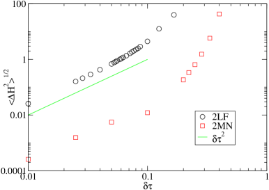
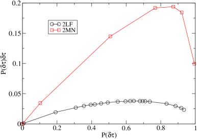
Fig. 1 shows the root mean square (RMS) of $\Delta H$ as a function of $\delta\tau$. Here the total integration length is set to 2. At small $\delta\tau$ the RMS of $\Delta H$ for both integrators is proportional to $\delta\tau^{2}$ as theoretically expected[19, 17]. As $\delta\tau$ increases higher order terms contribute the RMS of $\Delta H$ and the RMS of $\Delta H$ increases more rapidly with $\delta\tau$. The efficiency of the integrators can be measured by the efficiency function defined by $P(\delta\tau)\delta\tau$ where $P(\delta\tau)$ stands for the acceptance at $\delta\tau$. Fig.2 shows the efficiency function as a function of $P(\delta\tau)$. It is found that the efficiency function takes a maximum at a certain optimum acceptance $P_{opt}$. For the 2LFI, $P_{opt}$ is found to be around 0.65 which is consistent with the theoretical value 0.61[17] for the 2nd order integrators. On the other hand for the 2MNI, $P_{opt}$ is around $0.8\sim 0.9$ which is rather close to the optimum value for the higher order integrators[9]. This can be explained by that higher order error terms of the 2MNI dominate the RMS of $\Delta H$ already at lower $\langle\Delta H^{2}\rangle^{1/2}$. From fig.2 we see that the efficiency function of the 2MNI at the optimum is about 5 times bigger than that of the 2LFI. Since the computational cost of the 2MNI is 2 times bigger than that of the 2LFI[11], in total the 2MNI is about 2.5 times more efficient than the 2LFI.

Table 1 shows the results obtained by the MCMC simulations. Here the HMCA with the 2MNI is performed with $\delta\tau=0.222$ which corresponds to the optimum acceptance. We find that the results obtained by the MCMC simulations are consistent with the input values, which means that our MCMC algorithm worked correctly. The autocorrelation time (ACT), $2\tau_{int}$ is defined by $2\tau_{int}=1+2\sum_{t=1}^{\infty}ACF(t)$ where $ACF(t)$ stands for the autocorrelation function. In table 1 we only show the results of $h_{10}$ as a representative one for the volatility variables. $2\tau_{int}$ of $h_{10}$ is around $21$ which is very small compared to about 200 of the Metropolis algorithm[10].

Figure 1: $\langle\Delta H^{2}\rangle^{1/2}$ as a function of $\delta\tau$. The solid line shows a line proportional to $\delta\tau^{2}$.

Figure 2: The efficiency function $P(\delta\tau)\delta\tau$ versus $P(\delta\tau)$.

Table 1: Results obtained by MCMC simulations. S.D. stands for standard deviation.

	$\phi$	$\mu$	$\xi$	$\sigma_{\eta}^{2}$	$\sigma_{u}^{2}$	$h_{10}$
input	0.93	-1.0	0.3	0.1	0.2
average	0.926	-0.97	0.31	0.097	0.203	-9.77
S.D.	0.007	0.10	0.03	0.006	0.010	0.23
$2\tau_{int}$	8.8(20)	96(40)	1130(480)	64(18)	38(10)	21(6)

5 Empirical Study

As an empirical study we also performed the Bayesian inference of the RSV model for the stock price data of Panasonic Co. sampled from 3 July 2006 to 30 Dec. 2009 and estimated the model parameters of the RSV model. The RV is constructed by using 1min-sampling high-frequency returns. We use the 2MNI for the HMCA and set the step size to 0.1 and the total integration length to 1. We discarded the first 5000 MCMC samples and then accumulated 50000 samples for analysis.

Table 2 shows the results estimated from the MCMC simulation. The ACT of $h_{10}$ is found to be short, around 37. Thus MCMC samples of volatility variables are well de-correlated by the HMCA. The parameter $\xi$ corresponds to the bias correction of the RV[4]. The raw RV is distorted by bias such as microstructure noise and non-trading effects. To correct such bias Hansen and Lunde[20] introduced an adjustment factor $c$ which rescales the average of the RV to the variance of the daily returns. Using $c$, the raw $RV$ is corrected to $cRV$. If $\xi$ explains the same bias as the adjustment factor $c$ the relation $\xi=-\log(c)$ should hold. For the RV with 1min sampling frequency we obtain $c=1.244$, thus $-\log(c)=-0.2183$. On the other hand we obtain $\xi=-0.101$ which is considerably different from $-\log(c)$. Therefore this indicates that $\xi$ may also include other type of bias in the RV.

Table 2: Results obtained by MCMC simulations for Panasonic Co.

	$\phi$	$\mu$	$\xi$	$\sigma_{\eta}^{2}$	$\sigma_{u}^{2}$	$h_{10}$
average	0.958	-7.63	-0.101	0.0440	0.0176	-7.21
S.D.	0.013	0.14	0.049	0.0036	0.0031	0.12
$2\tau_{int}$	39(6)	24(0)	178(42)	65(11)	112(19)	37(11)

6 Conclusion

We have performed the Bayesian estimation of the RSV model by the HMCA. We find that the HMCA with the 2MNI is more efficient than the conventional 2LFI. We also find that the ACT of the volatility variables by the HMCA is short, which means that the HMCA can sample well de-correlated volatility variables. Finally we conclude that the HMCA with the 2MN integrator is efficient for the Bayesian parameter estimation of the RSV model.

References

- [1] Taylor S J 1986 Modelling Financial Time Series John Wiley & Sons, New Jersy
- [2] Andersen T G and Bollerslev T 1998 International Economic Review 39 885-905
- [3] Andersen T G, Bollerslev T, Diebold F X and Labys P 2001 J. Am. Statist. Assoc.A 96 42-55
- [4] Takahashi M, Omori Y and Watanabe T 2009 Compt. Stat. & Data anal. 53 2404-2425
- [5] Kim S, Shephard N and Chib S 1998 Review of Economic Studies 65 361-393
- [6] Shephard N and Pitt M K 1997 Biometrika 84 653-667
- [7] Watanabe T and Omori Y 2004 Biometrika 91 246-248
- [8] Duane S, Kennedy A D, Pendleton B J and Roweth D 1987 Phys. Lett. B 195 216-222
- [9] Takaishi T 2008 Lecture Notes in Computer Science 5226 929-936
- [10] Takaishi T 2009 Journal of Circuits, Systems, and Computers 18 1381-1396
- [11] Takaishi T 2013 J. Phys.: Conf. Ser. 423 012021
- [12] Omelyan I P, Mryglod I M and Folk R 2003 Comput. Phys. Commun. 151 272
- [13] Takaishi T and de Forcrand Ph 2008 Phys. Rev. E 73 036706
- [14] Montvay I and Münster G 1994 Quantum Fields on a Lattice Cambridge University Press
- [15] Forest E and Ruth R D 1990 Physica D 43 105-117
- [16] Yoshida H 1990 Phys. Lett. A 150 262-268
- [17] Takaishi T 2000 Comput. Phys. Commun. 133 6-17
- [18] Takaishi T 2002 Phys. Lett. B 540 159-165
- [19] Gupta S, Irbäck, Karsch F and Petersson B 1990 Phys. Lett. B 242 437
- [20] Hansen P R and Lunde A 2005 Journal of Applied Econometrics 20 873-889