The zero-patient problem with noisy observations

Abstract

A Belief Propagation approach has been recently proposed for the zero-patient problem in a SIR epidemics. The zero-patient problem consists in finding the initial source of an epidemic outbreak given observations at a later time. In this work, we study a harder but related inference problem, in which observations are noisy and there is confusion between observed states. In addition to studying the zero-patient problem, we also tackle the problem of completing and correcting the observations possibly finding undiscovered infected individuals and false test results.

Moreover, we devise a set of equations, based on the variational expression of the Bethe free energy, to find the zero patient along with maximum-likelihood epidemic parameters. We show, by means of simulated epidemics, how this method is able to infer details on the past history of an epidemic outbreak based solely on the topology of the contact network and a single snapshot of partial and noisy observations.

I Introduction

Epidemic compartment models provide a simple and useful mathematical description of the mechanisms behind disease transmission between individuals, in which only the most prominent ingredients are included Bailey (1975). One of the most celebrated of these models, Susceptible-Infected-Recovered (SIR)Kermack and McKendrick (1927), describes diseases in which the person contracting the disease becomes immune to future infections after recovery, such as measles, rubella, chicken pox and generic influenza. The same model can be applied to lethal diseases, such as HIV or Ebola, provided that the recovered state is replaced by a removed state. Being simple and mathematically appealing, models such as SIR can be employed to study under which conditions and with which consequences large epidemic outbreaks can occur. For most examples of infective diseases, contagion runs over a network of effective contacts between individuals. These contact networks have been inaccessible for decades, but thanks to recent advances in technology miniaturization (e.g. by means of RFID-endowed badges to signal the proximity between individuals) and the popularization of the Internet (e.g. for the construction of databases of self-reported interactions), at least in simple and controlled scenarios the interaction patterns of individual contacts can be almost entirely reconstructed Isella et al. (2011); Rocha et al. (2010). Modern computational epidemiology can thus rely on accurate data and on powerful computers to run large-scale simulations of stochastic compartment models on real contact networks Danon et al. (2011); Marathe and Vullikanti (2013).

In addition to epidemic forecast and control, a problem that has gained attention in recent years is the one of reconstructing the history of an epidemic outbreak Shah and Zaman (2010); Comin and da Fontoura Costa (2011); Shah and Zaman (2011); Fioriti and Chinnici (2012); Pinto et al. (2012); Antulov-Fantulin et al. (2013); Dong et al. (2013); Lokhov et al. (2013); Luo et al. (2013); Zhu and Ying (2013); Karamchandani and Franceschetti (2013); Altarelli et al. (2014), as e.g. the path of contagion to a specific infected individual. In particular, identifying the origin (or the set of seeds or sources) of an epidemic outbreak in the general case is an open problem, even assuming simple discrete-time stochastic epidemic models, such as the SI and SIR model. The reason becomes clear when the inference is formulated as a maximum likelihood estimation problem. Estimating the maximum of a properly defined likelihood function corresponds to solve a (generally non-convex) optimization problem in the space of all possible epidemic propagations that are compatible with the data. For propagations with a unique source on regular trees, a maximum likelihood estimator was proposed by Shah and Zaman Shah and Zaman (2010, 2011) under the name of rumor centrality (see also Dong et al. (2013)) and extended to probabilistic observations in Ref. Karamchandani and Franceschetti (2013). For a specific continuous-time epidemic process, an optimal estimator on general trees was put forward by Pinto et al. Pinto et al. (2012). On general graphs, the number of propagation paths grows exponentially with the number of nodes making the exact inference unfeasible in practice. Instead of evaluating the likelihood function, Zhu and Ying put forward a method to select the path that most likely leads to the observed snapshot Zhu and Ying (2013). For general graphs, other heuristic inference methods are based on centrality measures Comin and da Fontoura Costa (2011); Fioriti and Chinnici (2012), on the distance between observed data and typical outcome of propagations for given initial conditions Antulov-Fantulin et al. (2013) or on the assumption that the epidemic propagation follows a breadth-first search tree Pinto et al. (2012); Luo et al. (2013). Even fewer results exist for epidemic inference with multiple sources Luo et al. (2013). A message-passing approach for the computation of epidemic dynamics was first introduced by Karrer and Newman Karrer and Newman (2010) and applied to source detection in Ref. Lokhov et al. (2013), with a further mean-field approximation of the likelihood function.

Recently, a Belief Propagation (BP) approach was proposed for the Bayesian inference of the origin of an epidemics Altarelli et al. (2014). The main idea is that of exploiting a graphical model representation of the stochastic dynamics of the SI and SIR models to devise an efficient message-passing algorithm for the evaluation of the posterior distribution of the epidemic sources. The BP approach is exact on trees and it works very well also on general graphs, outperforming other methods on many graph topologies, in the presence of one or more sources, and also when observations are by large extent incomplete. In this work, we build on the BP approach by studying a harder variant of the inference problem in which either (a) it is not possible to distinguish between recovered or susceptible individuals or (b) the observation is noisy, i.e. there is a non-zero probability of making an error in the observation of each individual. The first case was already described in Ref. Zhu and Ying (2013) using the most likely infection path method on trees and similar heuristics on general graphs. The second case was not directly faced in the literature, although the problem of determining the causative network of epidemiological data in the presence of false negatives and positives has recently attracted some attention Milling et al. (2013); Meirom et al. (2014). We will show that the BP approach allows for more complete inference, as e.g. (a) to infer the epidemic parameters i.e. the probability of transmission in each contact and the distribution of recovery times; and (b) to infer missing data in a partial observation, e.g. correcting errors or finding which of the two states S, R in the confused state setup.

The work is organized as follows. Section 2 provides a detailed description of the graphical model representation of the stochastic epidemic dynamics. The BP equations of the model and the details of their efficient implementation are discussed in Section 3 (plus Appendices). The results of the Bayesian inference under different observation models are reported in Section 4. In Section 5, we present an efficient on-line method for the inference of the epidemic parameters by maximization of the log-likelihood by gradient ascent in the Bethe approximation.

II Graphical model representation of the epidemic process

We consider a discrete-time version of the susceptible-infected-recovered (SIR) model Kermack and McKendrick (1932) on a graph $G=(V,E)$ that represents the contact network of a set $V$ of individuals. A node $i$ can be in one of three possible states: susceptible $(S)$, infected $(I)$, and recovered/removed $(R)$. The state of node $i$ at time $t$ is represented by a variable $x_{i}^{t}\in\{S,I,R\}$. At each time step (e.g. a day) of the stochastic dynamics, an infected node $i$ can first spread the disease to each susceptible neighbor $j$ with given probability $\lambda_{ij}$, then recover with probability $\mu_{i}$. Once recovered, individuals do not get sick anymore. This process is Markovian, and satisfies $P(\mathbf{x}^{t+1}|\mathbf{x}^{t})=\prod_{i}P(x_{i}^{t+1}|\mathbf{x}^{t})$ where

$$P(x_{i}^{t+1}=S|\mathbf{x}^{t}) = \mathbb{I}[x_{i}^{t}=S]\prod_{j\in\partial i}(1-\lambda_{ji}\mathbb{I}[x_{j}^{t}=I])$$

$$P(x_{i}^{t+1}=I|\mathbf{x}^{t}) = (1-\mu_{i})\mathbb{I}[x_{i}^{t}=I]+\mathbb{I}[x_{i}^{t}=S](1-\prod_{j\in\partial i}(1-\lambda_{ji}\mathbb{I}[x_{j}^{t}=I]))$$

$$P(x_{i}^{t+1}=R|\mathbf{x}^{t}) = \mu_{i}\mathbb{I}[x_{i}^{t}=I]+\mathbb{I}[x_{i}^{t}=R].$$

A realization of the stochastic dynamics is fully specified by knowing for each individual $i$, her infection time $t_{i}=\min\{t:x_{i}^{t}=I\}$ and her recovery time $g_{i}=\min\{g:x_{i}^{t_{i}+g+1}=R\}$. It is easy to show that, for a given initial configuration $\{x_{i}^{0}\}$, a realization of the stochastic process can be generated by drawing randomly the recovery time $g_{i}$ of each node $i$ and an infection transmission delay $s_{ij}$ from node $i$ to node $j$, for all pairs $(ij)$. The recovery times $\{g_{i}\}$ are independent random variables extracted from geometric distributions $\mathcal{G}_{i}\left(g_{i}\right)=\mu_{i}\left(1-\mu_{i}\right)^{g_{i}}$, while the delays $\{s_{ij}\}$ are also independent random variables distributed according to a truncated geometric distribution,

$$\omega_{ij}\left(s_{ij}|g_{i}\right)=\begin{cases}\lambda_{ij}\left(1-\lambda_{ij}\right)^{s_{ij}},&s_{ij}\leq g_{i}\\ \sum_{s>g_{i}}\lambda_{ij}\left(1-\lambda_{ij}\right)^{s},&s_{ij}=\infty,\end{cases}$$

in which for convenience we concentrate in the value $s_{ij}=\infty$ the mass of the distribution beyond the hard cut-off $g_{i}$ imposed by the recovery time. Infection times are related by the deterministic equation

$$t_{i}=\min_{j\in\partial i}(t_{j}+s_{ji})+1$$ (1)

which is a constraint encoding the infection dynamics of the SIR model. Then individual $i$ recovers at time $t_{i}+g_{i}$.

The exact mapping from realizations of the epidemic process to realizations of the transmission delays and recovery times can be exploited to provide a graphical model representation of the stochastic dynamics of the SIR model on a graph. For a given initial condition, the joint probability distribution of infection and recovery times conditioned on the initial state is

$$\mathcal{P}\left(\mathbf{t},\mathbf{g}|\mathbf{x}^{0}\right) =\sum_{\mathbf{\{s_{ij}\}}}\mathcal{P}\left(\mathbf{s}|\mathbf{g}\right)\mathcal{P}\left(\mathbf{t}|\mathbf{x}^{0},\mathbf{g},\mathbf{s}\right)\mathcal{P\left(\mathbf{g}\right)}$$

$$=\sum_{\mathbf{\{s_{ij}\}}}\prod_{i,j}\omega_{ij}\left(s_{ij}|g_{i}\right)\prod_{i}\phi_{i}(t_{i},\{t_{k},s_{ki}\}_{k\in\partial i})\mathcal{G}_{i}(g_{i}),$$ (2)

where

$$\phi_{i}(t_{i},\{t_{k},s_{ki}\}_{k\in\partial i})=\delta(t_{i,}\mathbb{I}[x_{i}^{0}\neq I](\min_{k\in\partial i}(t_{k}+s_{ki})+1))$$ (3)

is a characteristic function which imposes on each node $i$ the dynamical constraint (1).

In the following we derive a method to reconstruct information about the origin of the epidemics given some observation at later times. We first need to compute the posterior probability of the initial configuration given an observation at time $T$. This is done by assuming to have a probabilistic prior on the initially infected nodes and by applying Bayes formula,

$$\mathcal{P}\left(\mathbf{x}^{0}|\mathbf{x}^{T}\right)\propto\sum_{\mathbf{t,g}}\mathcal{P}\left(\mathbf{x}^{T}|\mathbf{t},\mathbf{g}\right)\mathcal{P}\left(\mathbf{t},\mathbf{g}|\mathbf{x}^{0}\right)\mathcal{P}\left(\mathbf{x}^{0}\right)=\sum_{\mathbf{t},\mathbf{g},\mathbf{s}}\prod_{i,j}\omega_{ij}\prod_{i}\phi_{i}\mathcal{G}_{i}\gamma_{i}\zeta_{i}$$ (4)

where $\mathcal{P}\left(\mathbf{x}^{0}\right)=\prod_{i}\gamma_{i}\left(x_{i}^{0}\right)$ is a factorized prior on the initial infection and where we exploited the fact that the state $\mathbf{x}^{T}$ is a deterministic function of the set of infection and recovery times $(\mathbf{t},\mathbf{g})$ given by

$$\mathcal{P}\left(\mathbf{x}^{T}|\mathbf{t},\mathbf{g}\right)=\prod_{i}\zeta_{i}^{T}\left(t_{i},g_{i},x_{i}^{T}\right)$$ (5)

with

$$\zeta_{i}^{t}=\mathbb{I}\left[x_{i}^{t}=S,t<t_{i}\right]+\mathbb{I}\left[x_{i}^{t}=I,t_{i}\leq t<t_{i}+g_{i}\right]+\mathbb{I}\left[x_{i}^{t}=R,t_{i}+g_{i}\leq t\right].$$ (6)

The above formula can be generalized to the case in which the parameters $\mu$ and $\lambda$ have an explicit dependence on $t_{i}$. The problem of computing the marginals from (4) is in general intractable (NP-hard) and we need to resort to an efficient approximation. Here we choose to implement the BP approximation which preserves some non trivial correlations between variables and is exact in the limit cases in which correlation decay holds.

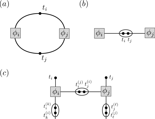
Figure 1: (a) Example of a loopy factor graph representations induced by constraints such as those in (1). (b) Disentangled factor graph. (c) A more convenient representation of the disentangled factor graph employed in the present work. For simplicity, the dependency on $\{s_{ij}\}$ is not considered.

We proceed by introducing a factor graph representation of (4), namely a bipartite graph composed of factor nodes and variable nodes. In the standard definition, each variable appearing in the problem is identified by a variable node, while each factorized term of the probability weight in (4) is represented by a factor node. A factor node is connected to the set of variable nodes appearing in the corresponding factorized term. However, with this definition the factor graph of (4) has a loopy structure both at local and global scale, and this could compromise the accuracy of the BP approximation. The existence of short loops can be easily verified even focusing only on the expression of the dynamical constraint (1): a pair of variable nodes corresponding to the infection times $t_{i}$ and $t_{j}$ of neighboring individuals are indeed involved in the two factors $\phi_{i}$ and $\phi_{j}$, inducing a short loop in the factor graph (see Fig.1a). We would like to use a factor graph representation that maintains the same topological properties of the original graph of contacts, in order to guarantee that BP is exact when the original graph of contacts is a tree. Following an approach proposed in Altarelli et al. (2013a, b), the factor graph can be disentangled by grouping pairs of infection times $(t_{i},t_{j})$ in the same variable node as in Fig.1b. For convenience, we will keep all variable nodes $\{t_{i}\}$ but we will also introduce for each edge $(i,j)$ emerging from a node $i$ a set of copies $t_{i}^{(j)}$ of the infection time $t_{i}$, that will be forced to take the common value $t_{i}$ (see Fig.1c) by including the constraint $\prod_{k\in\partial i}\delta(t_{i}^{(k)},t_{i})$ in the factor $\phi_{i}$.

We also observe that the factors $\phi_{i}$ depend on infection times and transmission delays just through the sums $t_{i}^{(j)}+s_{ij}$. It is thus more convenient to introduce the variables $t_{ij}=t_{i}^{(j)}+s_{ij}$ and express the dependencies through the pairs $(t_{i}^{(j)},t_{ij})$.

Finally it is convenient to group the variable $g_{i}$ with the corresponding infection times $t_{i}$ in the same variable node, replace $g_{i}$ and $g_{j}$ by their copies $g_{i}^{(j)}$ and $g_{j}^{(i)}$ in the edge constraints $\omega_{ij}(t_{ij}-t_{i}^{(j)}|g_{i}^{(i)})$ and $\omega_{ji}(t_{ji}-t_{j}|g_{j}^{(i)})$ and impose the identity $\prod_{k\in\partial i}\delta(g_{i}^{(k)},g_{i})$ for each node $i$.

We can now define the new factors

$$\phi_{ij}=\omega_{ij}(t_{ij}-t_{i}^{(j)}|g_{i}^{(i)})\omega_{ji}(t_{ji}-t_{j}^{(i)}|g_{j}^{(i)})$$ (7)

and

$$\psi_{i} =\delta(t_{i},\mathbb{I}[x_{i}^{0}\neq I](\min_{j\in\partial i}(t_{ji}+1)))\prod_{j\in\partial i}\delta(t_{i}^{(j)},t_{i})\text{$\delta$}(g_{i}^{(j)},g_{i})$$

$$=\phi_{i}(t_{i},\{{t}_{ji}\}_{j\in\partial i})\prod_{j\in\partial i}\delta(t_{i}^{(j)},t_{i})\text{$\delta$}(g_{i}^{(j)},g_{i}).$$ (8)

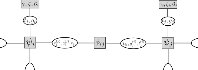
Figure 2: Factor graph representation of the graphical model associated with the distribution (10).

The posterior distribution can be written as

$$\mathcal{P}\left(\mathbf{x}^{0}|\mathbf{x}^{T}\right)\propto\sum_{\mathbf{{\bf}t},\{t_{ij}\},\mathbf{{\bf}g}}{\cal Q}({\bf g},{\bf t},\{t_{ij}\},x_{0})$$ (9)

where

$${\cal Q}({\bf g},{\bf t},\{t_{ij}\},x_{0})=\frac{1}{Z}\prod_{i<j}\phi_{ij}\prod_{i}\psi_{i}{\cal G}_{i}\gamma_{i}\zeta_{i}.$$ (10)

Figure 2 shows the factor graph representation of the distribution (10). The factor node grouping $\xi_{i},\zeta_{i}$ and $\mathcal{G}_{i}$ has in fact a more complex structure that is described in detail in Fig.3a: the function $\zeta_{i}^{t}$, defined in (6), connects the infection time $t_{i}$ with the state $x_{i}^{t}$ of the node at time $t$, $\gamma_{i}$ is the prior on the initial state, while $\mathcal{G}_{i}(g_{i})$ is the recovery time distribution. Having built a factor graph with the same topology of the original graph, we can now compute the exact posterior marginals for the SIR model with BP in the case of tree graphs and obtain a good approximation of it even on graphs that are not trees if the correlation decay assumption is correct.

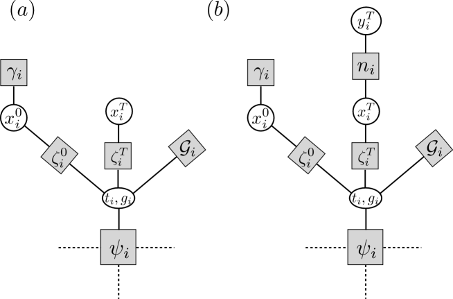
Figure 3: (a) Detailed description of the internal structure of the factor node containing $\gamma_{i},\zeta_{i},\mathcal{G}_{i}$ in Fig.2. (b) The modified factor graph used to include the observation models discussed in Section IV.

III BP Equations

Belief propagation consists in a set of equations for single-site probability distributions labeled by directed graph edges. These equations are solved by iteration, and on a fixed point give an approximation for single-site marginals and other quantities of interest like the partition function $Z$.

We recall the general form of the BP equations in the following. For a factorized probability measure on $\underline{z}=\{z_{i}\}$,

$$M(\underline{z})=\frac{1}{Z}\prod_{a}F_{a}(\underline{z}_{a})$$ (11)

where $\underline{z}_{a}$ is the subvector of variables that $F_{a}$ depends on, the general form of the equations is

$$p_{F_{a}\to i}\left(z_{i}\right) = \frac{1}{Z_{ai}}\sum_{\left\{z_{j}:j\in\partial a\setminus i\right\}}F_{a}\left(\left\{z_{i}\right\}_{i\in\partial a}\right)\prod_{j\in\partial a\setminus i}m_{j\to F_{a}}\left(z_{j}\right)$$ (12)

$$m_{i\to F_{a}}\left(z_{i}\right) = \frac{1}{Z_{ia}}\prod_{b\in\partial i\setminus a}p_{F_{b}\to i}\left(z_{i}\right)$$ (13)

$$m_{i}\left(z_{i}\right) = \frac{1}{Z_{i}}\prod_{b\in\partial i}p_{F_{b}\to i}\left(z_{i}\right)$$ (14)

where $F_{a}$ is a factor (i.e. $\psi_{i}$, $\phi_{ij}$, $\gamma_{i}$, $\zeta_{i}^{0}$, $\zeta_{i}^{T}$ or $\mathcal{G}_{i}$ in our case), $z_{i}$ is a variable (i.e. $(t_{i},g_{i})$, $(t_{i}^{\left(j\right)},g_{i}^{\left(j\right)},t_{ji})$, $x_{i}^{0}$ or $x_{i}^{T}$ in our case), $\partial a$ is the subset of indices of variables in factor $F_{a}$ and $\partial i$ is the subset of factors that depend on $z_{i}$. The terms $Z_{ia},Z_{ai}$ and $Z_{i}$ are normalization factors that can be calculated once the rest of the right-hand side is computed. While equations (13)-(14) can be always computed efficiently in general, the computation of the trace in (12) may need a time which is exponential in the number of participating variables. The update equations (12) for factors $\phi_{ij}$, $\gamma_{i}$, $\zeta_{i}^{0}$, $\zeta_{i}^{T}$ and $\mathcal{G}_{i}$ can be computed in a straightforward way because they involve a very small (constant) number of variables each. In Appendix A we show the derivation of an efficient version of equation (12) for factor $\psi_{i}$ that can be computed in linear time in the degree of vertex $i$, and we provide a change of variables that simplifies the messages and further reduces the computation time of the update.

IV Observation models

In the inference of the origin of epidemic propagations it is often assumed that the state of every node is known at the observation time $T$ with no uncertainty. This is also the case studied in Ref.Altarelli et al. (2014), where the BP approach for this problem was first introduced. In practice, every clinical test for determining the state of an individual is affected by some amount of error, and this possibility has to be taken into account in the inference problem. Therefore, it is realistic to assume that each observation carries some level of noise. We introduce a general concept of observation model for the inference problem, that allows dealing with several different cases of incomplete and noisy data using a common notation. We will assume that the noise level is known (as it is the case for the majority of clinical tests), and introduce a new variable ${y}^{T}_{i}\in\left\{S,I,R\right\}$ for the observed state of node $i$ and an additional evidence term that reflects the probability $n_{i}\left({y}^{T}_{i}|{x}^{T}_{i}\right)$ of the observed state ${y}^{T}_{i}$ given the true state ${x}^{T}_{i}$. In the factor graph, the observed-state variables ${y}^{T}_{i}$ are fixed to their value given by the experimental observation (by means of a delta function representing an infinite external field), while the true-state variables $x^{T}_{i}$ are traced over in the compatibility function $\zeta_{i}^{T}$. More explicitly, the modified factor graph shown in Fig. 3b, contains a $\zeta_{i}^{T}$ factor node attached to the true-state variable $x^{T}_{i}$, which is linked to the observed state ${y}^{T}_{i}$ (which is a constant) through the node $n_{i}\left({y}^{T}_{i}|x^{T}_{i}\right)$. The posterior distribution now takes the form:

$$\mathcal{P}\left(\mathbf{x}^{0}|\mathbf{y}^{T}\right)\propto\sum_{\mathbf{{\bf}x}^{T},\mathbf{{\bf}t},\mathbf{{\bf}t}_{ij},\mathbf{{\bf}g}}{\cal Q}^{\prime}({\bf x}^{T},{\bf g},{\bf t},{\bf t}_{ij},x_{0})$$ (15)

where

$${\cal Q}^{\prime}({\bf x}^{T},{\bf g},{\bf t},{\bf t}_{ij},x_{0})=\frac{1}{Z}\prod_{i<j}\phi_{ij}\prod_{i}\psi_{i}{\cal G}_{i}\gamma_{i}\zeta_{i}n_{i}.$$ (16)

In what follows, we introduce for convenience a map $\rho(s)$ from indices $i\in\{1,2,3\}$ into configurations of the $x$ variables, such that $\rho(1)=S,\leavevmode\nobreak\ \rho(2)=I,\leavevmode\nobreak\ \rho(3)=R$, and then define the observational transition matrix (OTM) $O^{(i)}_{s,t}$ whose elements are the transition probabilities:

$$O^{(i)}_{s,t}=n_{i}\left(\rho(s),\rho(t)\right).$$ (17)

The case in which observations are complete and noiseless corresponds to an identity matrix $O^{(i)}_{s,t}=\delta_{st}$. In the following sections, we will cover some interesting examples of applications of this scheme to confused and noisy observations. Note that, in this generalized scheme, we can also take into account the case of partial observations, by assuming a totally uniform OTM $O^{(i)}_{s,t}\equiv\frac{1}{3}$ for unobserved nodes.

IV.1 Inference of epidemic source from confused observations

In some situations, it could be hard to distinguish between nodes that already recovered from a disease and nodes that did not contract it at all. To take into account this fact, we follow the approach of Ref.Zhu and Ying (2013) and explore the efficiency of our inference machinery in a setting in which observations on Susceptible and Recovered nodes are confused. More specifically, we allow only two types of observed states $x_{i}^{T}\in\left\{I,N\right\}$, where $N$ stands for Not-Infected. This situation corresponds to choose the following OTM:

$$O^{(i)}=\left(\begin{array}[]{ccc}\frac{1}{2}&0&\frac{1}{2}\\ 0&1&0\\ \frac{1}{2}&0&\frac{1}{2}\end{array}\right).$$

We verified the performances of the BP algorithm on a completely uniform setting provided by random regular graphs with identical infection parameters $\left(\lambda,\mu\right)$ for all nodes and links. All epidemic propagations were initiated from a unique seed (the zero patient). For each node, the BP algorithm provides an estimate of the posterior probability that the node got infected at a certain time, and thus also the probability that the node was the origin of the epidemics. We can thus rank the nodes in decreasing order with respect of the estimated probability of being the origin of the observed epidemics: the position of the true origin in the ranking provided by the algorithm is a good measure of the efficacy of the method. In what follows, we indicate with $i_{0}$ the ranking of the true origin of the epidemics, and with $|G|$ the number of nodes in the graph $G$.

An important by-product of the algorithm is the ability to infer the true state of a node from the marginal of the infection time, providing in this way a method to “correct” observations. More precisely, in the present example we consider the problem of discriminating between Susceptible and Recovered nodes. An effective method for quantifying the accuracy of such binary classification problem is the Receiver Operating Characteristic (ROC) curve, namely a plot of the “true positive rate" against the “false positive rate". Constructing the ROC curve in the present case is very easy: we select the $N$ nodes and rank them on the base of their marginal $\mathcal{P}\left(t_{i}=\infty|\mathbf{x}^{0}\right)$, we then take one step upward in the ROC whenever a true positive case is encountered (${y}_{i}^{T}=x_{i}^{T}=S$) or one step rightward in case of a false positive (${y}_{i}^{T}\neq x_{i}^{T}$). We performed this discrimination analysis for each sample and then computed the average value of the area under the ROC curve, that gives indication of the fraction of correctly classified nodes. It turns out that the proposed algorithm can be effectively used as an ex-post-facto tool for discriminating Susceptible against Recovered individuals.

Figure 4 displays the average rank of the true infected site $i_{0}$, normalized to the network size $|G|$, for a set of $M=1000$ simulated epidemic propagations with $\lambda=0.6$ and $\mu=1$ on random regular graphs of size $N=1000$ and degree $d=4$ ($T=10$). The quantities of interest are plot as functions of the normalized epidemic size $N_{IR}=\frac{|I|+|R|}{|G|}$ (i.e. the fraction of infected or recovered sites), whose values are discretized with intervals of width equal to $0.05$. Note that in all the figures we show in the paper, we discarded the rare cases with very low epidemic size ($N_{IR}<0.3$ in Fig. 5, $N_{IR}<0.2$ elsewhere) where the number of infected is extremely low and the inference is practically unfeasible.

For each set of data, the symbols report the mean value obtained averaging over the samples belonging to that interval and the error bars indicate the corresponding standard deviation. The average fraction of Infected nodes and the fraction of samples in each bin are reported as a reference. The normalized average rank of the true origin is very low for all values of the normalized epidemic size, meaning that the algorithm is very effective in identifying the zero-patient. We also show the average ROC area, which reveals that the inference algorithm allows a very good discrimination between $S$ and $R$ nodes.

The same analysis for a random graph with power-law degree distribution, obtained using the Barabasi-Albert model Barabási and Albert (1999), is reported in Fig.5. When the observation time $T$ is sufficiently small ($T=7$ in Fig.5), the performance of the algorithm is high. When longer observation times are considered, epidemics tend to cover the whole network and convergence issues emerge. In this regime, most of the infected nodes have already recovered at the observation time $T$ (and thus they cannot be distinguished anymore from the susceptible ones). This causes a rapid decay of the available information content that explains the performance degradation. A similar effect arises also on random regular graphs, but at longer times, as we will see in Section IV.2.

In summary, even when supplied with confused observations, BP shows striking ability to discriminate between Recovered and Susceptible nodes, provided that there is enough information at the chosen observation time $T$.

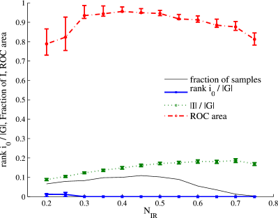
Figure 4: Average normalized rank of the true zero-patient (blue solid line), average ROC area (red dashed line) and average fraction of Infected nodes $\frac{|I|}{|G|}$ (green dotted line) as a function of the rescaled epidemic size $\frac{|I|+|R|}{|G|}$. The fraction of the $M$ samples belonging to each bin of the rescaled epidemic size is also indicated. The realization of the epidemic process is propagated for $T=10$ steps with $\lambda=0.6$ and $\mu=1$. Observations are confused, i.e. $x_{i}^{t}\in\left\{I,N\right\}$. Simulations were run over $M=1000$ samples of random regular graphs with $N=1000$ nodes and degree $d=4$.

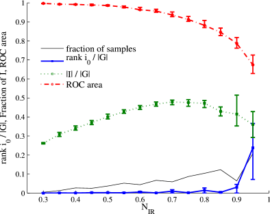
Figure 5: Average normalized rank of the true zero patient (blue solid line), average ROC area (red dashed line) and average fraction of Infected nodes $\frac{|I|}{|G|}$ (green dotted line) as a function of the rescaled epidemic size $\frac{|I|+|R|}{|G|}$. The fraction of the $M$ samples belonging to each bin of the rescaled epidemic size is also indicated. The realization of the epidemic process is propagated up to the time step $T=7$ with $\lambda=0.6$ and $\mu=0.5$. Observations are confused, i.e. $x_{i}^{t}\in\left\{I,N\right\}$. Simulations were run over $M=1000$ samples of Barabasi-Albert graphs with $N=1000$ nodes and average degree $\hat{d}=4$.

IV.2 Inference of the epidemic source with noisy observations

Let us now consider a simple type of observational noise. Suppose that a node on state $x$, has probability $1-\nu$ of being correctly observed in state $x$, and probability $\nu$ of being observed incorrectly in one of the two remaining states, distributed uniformly among the two. For example, node $i$ could be $I$ (Infected) at the observation time $T$, and, for a given noise level $\nu$, there will be an equal probability $\frac{\nu}{2}$ for node $i$ to be observed in the $R$ (Recovered) or $S$ (Susceptible) state. This setting corresponds to the following OTM:

$$O^{(i)}=\left(\begin{array}[]{ccc}1-\nu&\frac{\nu}{2}&\frac{\nu}{2}\\ \frac{\nu}{2}&1-\nu&\frac{\nu}{2}\\ \frac{\nu}{2}&\frac{\nu}{2}&1-\nu\end{array}\right).$$

We simulated a set of $M=1000$ single-source epidemic propagations with $\lambda=0.6$ and $\mu=1$ on random regular graphs with $N=1000$ nodes and degree $d=4$. In Fig. 6 we show the average rank of the true origin of the epidemics for various levels of the observational noise up to $\nu=0.4$. The low values of the average rank obtained demonstrate that the BP algorithm is able to perform extremely well up to very high levels of noise. The corresponding ROC curves are plotted in Fig. 7.

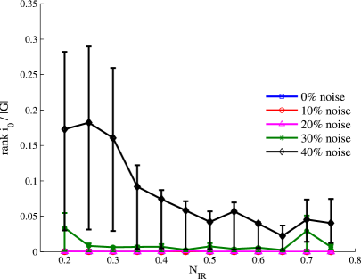
Figure 6: Average normalized rank of the true zero patient as a function of epidemic size $\frac{|I|+|R|}{|G|}$ for various levels of noise $\nu$ in the observation (the error-bars indicate the standard deviation computed on the sub-sample corresponding to a given epidemic size). Each curve refers to $M=1000$ samples of Random Regular graphs with $N=1000$ nodes and degree $d=4$. Epidemics is propagated until $T=10$ with $\lambda=0.6$ and $\mu=1$.

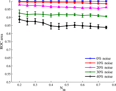
Figure 7: Average area of the ROC curve as a function of epidemic size $\frac{|I|+|R|}{|G|}$ for various levels of noise $\nu$ in the observation (the error-bars indicate the standard deviation computed on the sub-sample corresponding to a given epidemic size). Each curve refers to $M=1000$ samples of Random Regular graphs with $N=1000$ nodes and degree $d=4$. Epidemics is propagated until $T=10$ with $\lambda=0.6$ and $\mu=1$.

We investigated the role of observation time $T$ in relation to the amount of information needed for inferring the zero patient: simulations were run for given realizations of the epidemic process and observation time was systematically varied. In Fig. 8 we show a representative situation in random graphs (the picture is similar in scale-free graphs, as we argued in SectionIV.1). It turns out that the ratio of infected nodes to epidemic size is critical for inference: when observation time is too long so that the majority of infected individuals have recovered, it is much more difficult to find the zero-patient in the noisy and confused case. As it can be seen in the figure, this sharp change of behaviour (manifested at $T=11$) is present even in single instances.

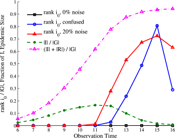
Figure 8: Normalized rank of the true zero-patient (solid lines), fraction of Infected nodes $\frac{|I|}{|G|}$ (green dotted line) and rescaled epidemic size $\frac{|I|+|R|}{|G|}$ (dotted purple line) as a function of observation time $T$ for a single realization of the epidemic process, propagated with $\lambda=0.6$ and $\mu=1$, on a random regular graph with $N=1000$ nodes and degree $d=4$. Observations are complete (black solid line, superimposed to x axes), confused (blue solid line), and with noise $20\%$ noise level (red solid line). Values of the normalized rank greater than $0.5$ are meaningless: they are the realization of a random variable with average close to 0.5, and they are evidence that for large $T$ the inference algorithm is unable to identify the zero-patient with better precision than pure chance.

V Inference of Epidemic Parameters

We have shown that if the parameters of the epidemics are known in advance, our inference method can effectively detect the zero patient. It is reasonable to assume that, for certain types of diseases, clinical information could dictate some plausible range for the average rates of infection and recovery. In the simplified case in which the infection parameters are uniform among the population, the BP method can be generalized in a way to infer both the zero patient and the epidemic parameters at the same time.

From our bayesian approach, $-f(\lambda,\mu)=\log Z(\lambda,\mu)$ is the log-likelihood of the epidemic parameters for the observation $\mathbf{x}^{T}$. Indeed, the log–likelihood of the parameters $-f(\lambda,\mu)$ equals $\log\mathcal{P}\left(\mathbf{x}^{T}|\lambda,\mu\right)$ and the latter can be computed as

$$\mathcal{P}\left(\mathbf{x}^{T}|\lambda,\mu\right)=\sum_{\mathbf{t,g,x^{0}}}\mathcal{P}\left(\mathbf{x}^{T}|\mathbf{t},\mathbf{g}\right)\mathcal{P}\left(\mathbf{t},\mathbf{g}|\mathbf{x}^{0}\right)\mathcal{P}\left(\mathbf{x}^{0}\right)=Z\left(\lambda,\mu\right).$$ (18)

In Ref. Altarelli et al. (2014), this observation was used to infer the epidemic parameters through an exaustive search in the space of parameters. This computation can be costly, wasting resources on noninteresting regions of the parameter space. Moreover, this type of experiments shows that the log-likelihood landscape with the Bethe approximation is generally very simple, presenting in most cases a single local maximum. Here we describe a different method to infer the parameters together with the source of the epidemic outbreak. The idea is to perform an on-line log-likelihood maximization through gradient ascent in the Bethe approximation of the log-likelihood, by means of the following updates:

$$\lambda \leftarrow \lambda+\epsilon\frac{\partial f}{\partial\lambda}$$ (19)

$$\mu \leftarrow \mu+\epsilon\frac{\partial f}{\partial\mu}$$ (20)

with $\epsilon$ a free convergence parameter. The free energy of the system can be approximated with the Bethe free energy, which in turn can be expressed as a sum of local terms depending on BP messages. A detailed derivation of the expression of the derivatives $\frac{\partial f}{\partial\lambda}$ and $\frac{\partial f}{\partial\mu}$ of the Bethe free energy is reported in Appendix B. In principle, the expressions obtained using the Bethe free energy are valid only at the BP fixed point, and one should let BP updates converge before making a step of gradient ascent. In practice, we found that it is sufficient to interleave BP and gradient ascent updates in order to obtain equivalent results. A fixed point of the interleaved updates is both a critical point of the Bethe log-likelihood and a BP approximation for the marginals. We performed extensive simulations with a wide range of parameters and found that, for reasonable fraction of infected nodes at the observation time, the inference can simultaneously identify the zero patient perfectly and find good estimates of the epidemic parameters. Some examples of inferred parameters are shown in Fig. 9 for six different configurations of $\left(\lambda,\mu\right)$ parameters, with each pair of box plots referring to $M=1000$ samples.

The method can be extended to treat the non-uniform case, at the expense of a higher computational effort, that would amount in computing local derivatives of the free-energy function for each edge in the graph with respect to edge-specific parameter. It should be clear that the number of parameters in the non-uniform case should not grow excessively for inference purposes: we could, nevertheless, account for age or gender-dependent differences in the probability to contract the disease or in the recovery rate with the introduction of additional information, attached to nodes and edges in the network. Notice that, even in this case, an exhaustive search in the parameter space could be computationally too expensive.

The inference of parameters can be performed also in the presence of observational noise. In Fig. 10 we show an example of inference for increasing levels of noise in the observation, as defined in the preceeding section. Also in this case the zero patient is detected with probability $1$ and the inferred parameters are good estimators of the true values even up to a significant fraction of noise.

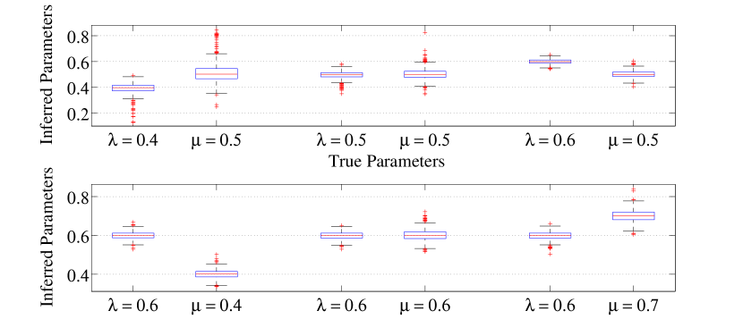
Figure 9: Inferred epidemic parameters for six different configurations of true $\left(\lambda,\mu\right)$ parameters. Forward epidemic is simulated until observation time $T=10$. Each pair of boxes refers to $M=1000$ instances of Random Regular graphs with $N=1000$ nodes and degree $g=4$. Box edges signal the $25$th and $75$th percentiles, the central red lines is the median. Whiskers extend to cover $99.3\%$ of the data for a gaussian distribution. Outliers are marked as red points outside the whiskers.

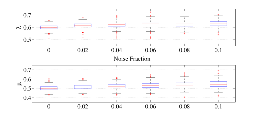
Figure 10: Inferred epidemic parameters for different observational noise rates $\nu$. Forward epidemic is simulated until observation time $T=10$. Each box refers to $M=1000$ instances of Random Regular graphs with $N=1000$ nodes and degree $g=4$. Box edges signal the $25$th and $75$th percentiles, the central red lines is the median. Whiskers extend up to cover $99.3\%$ of the data for a gaussian distribution. Outliers are marked as red points outside the whiskers.

We compared the ability of BP to infer the epidemic parameters with a simpler (though computationally expensive) procedure that does not require (nor provide) the simultaneous inference of the origin. The idea is to compare the statistical properties of the observation with the one of typical epidemics with given parameters $\lambda,\mu$, and choose those $\lambda,\mu$ that give properties that are closest (in a sense to be defined) to the ones observed. More precisely, for each $\lambda\in\{0.05,0.1,\dots,0.95\}$ and $\mu\in\{0,0.05,\dots,1\}$, we generate 1000 random epidemics and compute the mean of the number of infected $I_{mean}(\lambda,\mu)$ and recovered $R_{mean}(\lambda,\mu)$ individuals. Afterwards, given an observation with $I$ infected and $R$ recovered individuals, we find

$$(\lambda^{*},\mu^{*})=\arg\min_{\lambda,\mu}(I-I_{mean}(\lambda,\mu))^{2}+(R-R_{mean}(\lambda,\mu))^{2}.$$

We also repeated the procedure using the $median$ instead of the mean (and computing thus $I_{median}$ and $R_{median}$). In Fig. 11 we show the distributions of $\lambda^{*}$ and $\mu^{*}$ found by the above procedure based on 200 epidemic realizations with $\lambda=0.6$ and $\mu=0.5$, along by the same distribution as found by the interleaved BP gradient ascent of the likelihood function. The results show that the BP-based procedure is able to infer the correct parameter $\lambda=0.6$ and $\mu=0.5$ with much higher accuracy.

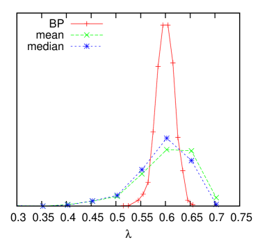
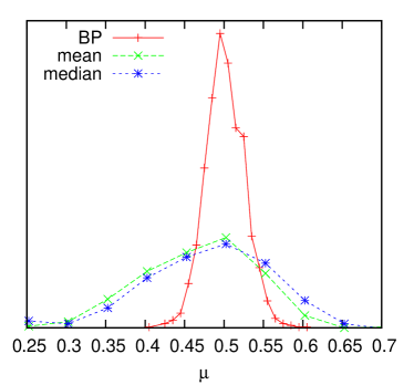
Figure 11: Comparison of inference of epidemic parameters for $200$ random realizations with $\lambda=0.6$, $\mu=0.5$ between BP and the naive method consisting in finding the couple $(\lambda^{*},\mu^{*})$ which is closest in terms of mean (resp. median) number of infected and recovered individuals in euclidean distance. The distributions for the inference with BP correspond to the fifth example reported in Fig.9 and the first in Fig.10.

VI Conclusion

BP was recently proposed as an efficient tool for the inference of the origins of an epidemic propagation on graphs from a snapshot of the system at a later time. In the present work, we generalized the analysis to more realistic cases in which observations are imperfect. Experimental results show that BP performs well even in the presence of strong sources of uncertainty, such as observational noise, inability to distinguish between observed states, and uncertainty on the intrinsic model parameter. We provided an exact solution on acyclic graphs for the first two problems, and a variational solution to compute the gradient of the likelihood of the parameters. The latter can be employed to find local maxima of the likelihood function. We also characterized, by means of simulations, the amount of information that can be extracted on random graphs of various types, both on the past origin of the epidemics and on the missing bits on the present-time observation. Besides giving an excellent algorithmic answer to these questions, related to the past and the present of an observed epidemics, the scheme can be easily generalized to give accurate predictions about the future evolution of an outbreak from which only a partial observation (noisy and/or incomplete) of the current state is available. Work is in progress in this direction.

Appendix A Efficient BP updates

An efficient form for the update equations of the $\psi_{i}$ factor nodes is the following:

$$p_{\psi_{i}\to j}\left(t_{i}^{\left(j\right)},t_{ji},g_{i}^{\left(j\right)}\right) \propto \sum_{g_{i},t_{i}}\sum_{\left\{t_{i}^{\left(k\right)},t_{ki},g_{i}^{\left(k\right)}\right\}}m_{i\to\psi_{i}}\left(t_{i},g_{i}\right)\times$$

$$\times\prod_{k\in\partial i\setminus j}m_{k\to\psi_{i}}\left(t_{i}^{\left(k\right)},t_{ki},g_{i}^{\left(k\right)}\right)\psi_{i}\left(t_{i},g_{i},\left\{\left(t_{i}^{(k)},t_{ki},g_{i}^{(k)}\right)\right\}_{k\in\partial i}\right)$$

$$\propto m_{i\to\psi_{i}}\left(t_{i}^{\left(j\right)},g_{i}^{\left(j\right)}\right)\sum_{t_{ki}}\prod_{k\in\partial i\setminus j}m_{k\to\psi_{i}}\left(t_{i}^{\left(j\right)},t_{ki},g_{i}^{\left(j\right)}\right)\times$$

$$\times\left[\delta\left(t_{i}^{(j)},0\right)+\delta\left(t_{i}^{(j)},\left(1+\min_{k\in\partial i}\left\{t_{ki}\right\}\right)\right)\right]$$

$$\propto \delta\left(t_{i}^{\left(j\right)},0\right)m_{i\to\psi_{i}}\left(0,g_{i}^{\left(j\right)}\right)\prod_{k\in\partial i\setminus j}\sum_{t_{ki}}m_{k\to\psi_{i}}\left(0,t_{ki},g_{i}^{\left(j\right)}\right)+$$

$$+\;m_{i\to\psi_{i}}\left(t_{i}^{\left(j\right)},g_{i}^{\left(j\right)}\right)\mathbb{I}\left(t_{i}^{\left(j\right)}\leq t_{ji}+1\right)\prod_{k\in\partial i\setminus j}\sum_{t_{ki}\geq t_{i}^{\left(j\right)}-1}m_{k\to\psi_{i}}\left(t_{i}^{\left(j\right)},t_{ki},g_{i}^{\left(j\right)}\right)$$

$$-\;m_{i\to\psi_{i}}\left(t_{i}^{\left(j\right)},g_{i}^{\left(j\right)}\right)\mathbb{I}\left(t_{i}^{\left(j\right)}<t_{ji}+1\right)\prod_{k\in\partial i\setminus j}\sum_{t_{ki}>t_{i}^{\left(j\right)}-1}m_{k\to\psi_{i}}\left(t_{i}^{\left(j\right)},t_{ki},g_{i}^{\left(j\right)}\right)$$

where in (A) we use the fact that

$$\delta\left(t_{i},\left(1+\min_{j\in\partial i}\left\{t_{ji}\right\}\right)\right)=\prod_{j\in\partial i}\mathbb{I}\left(t_{i}\leq t_{ji}+1\right)-\prod_{j\in\partial i}\mathbb{I}\left(t_{i}<t_{ji}+1\right).$$

It is also possibile to use a simpler representation for the messages, in which we just retain information on the relative timing of infection time $t_{i}^{\left(j\right)}$ for a node $i$ and infection propagation time $t_{ji}$ on its link with node $j$, introducing the variables $\sigma_{ji}=1+\mbox{sign}\left(t_{ji}-\left(t_{i}^{\left(j\right)}-1\right)\right)$.

In equation (A) we can easily group the sums over different configurations of $\left(t_{ki},t_{i}^{(j)}\right)$ and write:

$$p_{\psi_{i}\to j}\left(t_{i}^{\left(j\right)},\sigma_{ji},g_{i}^{\left(j\right)}\right) \propto \delta\left(t_{i}^{\left(j\right)},0\right)m_{i\to\psi_{i}}\left(0,g_{i}^{\left(j\right)}\right)\prod_{k\in\partial i\setminus j}\sum_{\sigma_{i}^{{}^{\prime}\left(k\right)}}m_{k\to\psi_{i}}\left(0,\sigma_{ki},g_{i}^{\left(j\right)}\right)+$$

$$+\;m_{i\to\psi_{i}}\left(t_{i}^{\left(j\right)},g_{i}^{\left(j\right)}\right)\mathbb{I}\left(\sigma_{ji}=1,2\right)\prod_{k\in\partial i\setminus j}\sum_{\sigma_{ki}=1,2}m_{k\to\psi_{i}}\left(t_{i}^{\left(j\right)},\sigma_{ki},g_{i}^{\left(j\right)}\right)$$

$$-\;m_{i\to\psi_{i}}\left(t_{i}^{\left(j\right)},g_{i}^{\left(j\right)}\right)\mathbb{I}\left(\sigma_{ji}=2\right)\prod_{k\in\partial i\setminus j}m_{k\to\psi_{i}}\left(t_{i}^{\left(j\right)},2,g_{i}^{\left(j\right)}\right)$$

Similarly, the outgoing message to the $i$ variable node is:

$$p_{\psi_{i}\to i}\left(t_{i},g_{i}\right) \propto \delta\left(t_{i},0\right)\prod_{k\in\partial i}\sum_{\sigma_{ki}}m_{k\to\psi_{i}}\left(0,\sigma_{ki},g_{i}\right)+$$

$$+\prod_{k\in\partial i}\sum_{\sigma_{ki}=1,2}m_{k\to\psi_{i}}\left(t_{i},\sigma_{ki},g_{i}\right)$$

$$-\prod_{k\in\partial i}m_{k\to\psi_{i}}\left(t_{i},2,g_{i}\right)$$

In the simplified  $\left(t,\sigma,g\right)$ representation for the messages, the update equation for the $\phi_{ij}$ nodes can be written in an easy way:

$$p_{\phi_{ij}\to j}\left(t_{j},\sigma_{ij},g_{j}\right)\propto\sum_{t_{i},\sigma_{ji},g_{i}}\Omega\left(t_{i},t_{j},\sigma_{ij},\sigma_{ji},g_{i},g_{j}\right)p_{i\to\phi_{ij}}\left(t_{i},\sigma_{ji},g_{i}\right)$$ (26)

where:

$$\Omega\left(t_{i},t_{j},\sigma_{ij},\sigma_{ji},g_{i},g_{j}\right)=\begin{cases}\chi\left(t_{i},t_{j},\sigma_{ij},g_{i}\right)&:t_{i}<t_{j},\leavevmode\nobreak\ \sigma_{ji}=2,\leavevmode\nobreak\ \sigma_{ij}\neq 2\\ \chi\left(t_{i},t_{j},\sigma_{ij},g_{i}\right)+\left(1-\lambda\right)^{g_{i}+1}&:t_{i}<t_{j},\leavevmode\nobreak\ \sigma_{ji}=2,\leavevmode\nobreak\ \sigma_{ji}=2\\ \chi\left(t_{j},t_{i},\sigma_{ji},g_{j}\right)&:t_{j}<t_{i},\leavevmode\nobreak\ \sigma_{ji}=2,\leavevmode\nobreak\ \sigma_{ji}\neq 2\\ \chi\left(t_{j},t_{i},\sigma_{ji},g_{j}\right)+\left(1-\lambda\right)^{g_{j}+1}&:t_{j}<t_{i},\leavevmode\nobreak\ \sigma_{ij}=2,\leavevmode\nobreak\ \sigma_{ji}=2\\ 1&:t_{i}=t_{j},\leavevmode\nobreak\ \sigma_{ji}=\sigma_{ij}=2\\ 0&:otherwise\end{cases}$$ (27)

and

$$\chi\left(t_{1},t_{2},\sigma,g\right)=\sum_{t=t_{1}}^{t_{1}+g}\delta\left(\sigma\left(t_{2},t\right),\sigma\right)\lambda\left(1-\lambda\right)^{t-t_{1}}$$ (28)

Note that it is possible to exploit the symmetry in $i$ and $j$ between the rows 1-2 and rows 3-4 in the definition (27) for $\Omega$: when one loops over the variables $\left(t_{j},\sigma_{ij},g_{j}\right)$ in order to fill in the output message $p_{\phi_{ij}\to j}\left(t_{j},\sigma_{ij},g_{j}\right)$, this consists in looping over the variables $\left(t_{j},\sigma_{ij},g_{j}\right)$ of the input message $p_{i\to\phi_{ij}}\left(t_{i},\sigma_{i},g_{i}\right)$, just with a switch in indices. In the implementation, this amounts in a significant reduction of a factor $G$ in the computational complexity for updates involving the factor node $\phi_{ij}$.

Appendix B Gradient ascent method for the inference of the epidemic parameters

The free energy of the system can be approximated with the Bethe free energy that can be expressed as a sum of local terms depending on the BP messages.

$$-f=\sum_{a}f_{a}+\sum_{i}f_{i}-\sum_{(ia)}f_{(ia)}$$ (29)

where

$$f_{a} = \log\left(\sum_{\left\{z_{i}:i\in\partial a\right\}}F_{a}\left(\left\{z_{i}\right\}_{i\in\partial a}\right)\prod_{i\in\partial a}m_{i\to a}(z_{i})\right)$$ (30)

$$f_{(ia)} = \log\left(\sum_{z_{i}}m_{i\to a}(z_{i})p_{F_{a}\to i}(z_{i})\right)$$ (31)

$$f_{i} = \log\left(\sum_{z_{i}}\prod_{b\in\partial i}p_{F_{b}\to i}(z_{i})\right)$$ (32)

The computation of the gradient of the free energy deserves some special attention: being $f$ a function of all the BP messages, one would argue that this messages depend on the model parameters too, at every step in the BP algorithm. Actually, there is no need to consider this implicit $(\lambda,\mu)$ dependence if BP has reached its fixed point, that is when BP equations are satisfied and the messages are nothing else but Lagrange multipliers with respect to the constraint minimization of the Bethe free energy functional Yedidia et al. (2001). In our scheme, the only explicit dependence of free energy on epidemic parameters is in the factor node terms $f_{a}$’s involving compatibility functions $\phi_{ij}=\omega_{ij}\left(t_{ij}-t_{i}|g_{i}\right)\omega_{ji}\left(t_{ji}-t_{j}|g_{j}\right)$ and $\mathcal{G}_{i}\left(g_{i}\right)=\mu_{i}\left(1-\mu_{i}\right)^{g_{i}}$, and the gradient can be computed very easily. For the $\phi_{ij}$ nodes we have:

$$\frac{\partial f_{\phi_{ij}}}{\partial\lambda}=\frac{\sum_{t_{i},t_{ji},g_{i},t_{j},t_{ij},g_{j}}\frac{\partial\phi_{ij}}{\partial\lambda}\left(t_{i},t_{ji},g_{i},t_{j},t_{ij},g_{j}\right)m_{i\to\phi_{ij}}\left(t_{i},t_{ji},g_{i}\right)m_{j\to\phi_{ij}}\left(t_{j},t_{ij},g_{j}\right)}{\sum_{t_{i},t_{ji},g_{i},t_{j},t_{ij},g_{j}}\phi_{ij}\left(t_{i},t_{ji},g_{i},t_{j},t_{ij},g_{j}\right)m_{i\to\phi_{ij}}\left(t_{i},t_{ji},g_{i}\right)m_{j\to\phi_{ij}}\left(t_{j},t_{ij},g_{j}\right)}$$ (33)

where

$$\frac{\partial\phi_{ij}}{\partial\lambda}=\begin{cases}1&t_{i}<t_{j}\mbox{ and }t_{i}=t_{ij}<t_{i}+g_{i}\\ -\left(g_{i}-t_{i}\right)\lambda\left(1-\lambda\right)^{g_{i}-t_{i}-1}&t_{i}<t_{j}\mbox{ and }t_{i}<t_{ij}=t_{i}+g_{i}\\ \left(1-\lambda\right)^{t_{ij}-t_{i}}-\left(t_{ij}-t_{i}\right)\lambda\left(1-\lambda\right)^{t_{ij}-t_{i}-1}&t_{i}<t_{j}\mbox{ and }t_{i}<t_{ij}<t_{i}+g_{i}\\ 1&t_{j}<t_{i}\mbox{ and }t_{j}=t_{j}<t_{j}+g_{j}\\ -\left(g_{j}-t_{j}\right)\lambda\left(1-\lambda\right)^{g_{j}-t_{j}-1}&t_{j}<t_{i}\mbox{ and }t_{j}<t_{ji}=t_{j}+g_{j}\\ \left(1-\lambda\right)^{t_{ji}-t_{j}}-\left(t_{ji}-t_{j}\right)\lambda\left(1-\lambda\right)^{t_{ji}-t_{j}-1}&t_{j}<t_{i}\mbox{ and }t_{j}<t_{ji}<t_{j}+g_{j}\\ 0&\mbox{else}\end{cases}$$ (34)

In the simplified $\left(t,\sigma,g\right)$ representation for the messages, equation (34) takes the form:

$$\frac{\partial\phi_{ij}}{\partial\lambda}=\begin{cases}\chi\left(t_{i},t_{j},\sigma_{ij},g_{i}\right)&t_{i}<t_{j},\sigma_{ji}=2,\sigma_{ij}\neq 2\\ \chi\left(t_{i},t_{j},\sigma_{ij},g_{i}\right)-\left(g_{i}+1\right)\left(1-\lambda\right)^{g_{i}}&t_{i}<t_{j},\sigma_{ji}=2,\sigma_{ij}=2\\ \chi\left(t_{j},t_{i},\sigma_{ji},g_{j}\right)&t_{j}<t_{i},\sigma_{ji}=2,\sigma_{ij}\neq 2\\ \chi\left(t_{j},t_{i},\sigma_{ji},g_{j}\right)-\left(g_{j}+1\right)\left(1-\lambda\right)^{g_{j}}&t_{j}<t_{i},\sigma_{ji}=2,\sigma_{ij}=2\\ 0&otherwise\end{cases}$$ (35)

where:

$$\chi\left(t_{1},t_{2},\sigma,g\right)=\sum_{t=t_{1}}^{t_{1}+g}\delta\left(\sigma\left(t_{2},t\right),\sigma\right)\left(1-\lambda\right)^{t-t_{1}}-\left(t-t_{1}\right)\lambda\left(1-\lambda\right)^{t-t_{1}-1}$$ (36)

For the $\mathcal{G}_{i}$ nodes we have:

$$\frac{\partial f_{\mathcal{G}_{i}}}{\partial\mu}=\frac{\sum_{g_{i}}\mathcal{\tilde{G}}_{i}(g_{i})m_{i\to\mathcal{G}_{i}}(g_{i})}{\sum_{g_{i}}\mathcal{G}_{i}(g_{i})m_{i\to\mathcal{G}_{i}}(g_{i})}$$ (37)

where

$$\mathcal{\tilde{G}}_{i}(g_{i})=\begin{cases}\left(1-\mu\right)^{g_{i}}-g_{i}\mu\left(1-\mu\right)^{g_{i}-1}&:g_{i}<G\\ G-G\left(1-\mu\right)^{G-1}&:g_{i}=G.\end{cases}$$ (38)

References

- Bailey (1975) N. T. J. Bailey, The mathematical theory of infectious diseases and its applications (Griffin, London, 1975).
- Kermack and McKendrick (1927) W. Kermack and A. McKendrick, “A contribution to the mathematical theory of epidemics,” Proceedings of the Royal Society of London. Series A 115, 700 (1927).
- Isella et al. (2011) L. Isella, J. Stehlé, A. Barrat, C. Cattuto, J.-F. Pinton, and W. Van den Broeck, “What’s in a crowd? analysis of face-to-face behavioral networks,” Journal of Theoretical Biology 271, 166 (2011).
- Rocha et al. (2010) L. E. C. Rocha, F. Liljeros, and P. Holme, “Information dynamics shape the sexual networks of internet-mediated prostitution,” PNAS 107, 5706 (2010), PMID: 20231480.
- Danon et al. (2011) L. Danon, A. P. Ford, T. House, C. P. Jewell, M. J. Keeling, G. O. Roberts, J. V. Ross, and M. C. Vernon, “Networks and the epidemiology of infectious disease,” Interdisciplinary perspectives on infectious diseases 2011 (2011).
- Marathe and Vullikanti (2013) M. Marathe and A. K. S. Vullikanti, “Computational epidemiology,” Commun. ACM 56, 88 (2013).
- Shah and Zaman (2010) D. Shah and T. Zaman, “Detecting sources of computer viruses in networks: theory and experiment,” SIGMETRICS 38, 203–214 (2010).
- Comin and da Fontoura Costa (2011) C. H. Comin and L. da Fontoura Costa, “Identifying the starting point of a spreading process in complex networks,” Phys. Rev. E 84, 056105 (2011).
- Shah and Zaman (2011) D. Shah and T. Zaman, “Rumors in a network: Who’s the culprit?” IEEE Trans Inf Theory 57, 5163–5181 (2011).
- Fioriti and Chinnici (2012) V. Fioriti and M. Chinnici, “Predicting the sources of an outbreak with a spectral technique,” arXiv preprint arXiv:1211.2333 (2012).
- Pinto et al. (2012) P. C. Pinto, P. Thiran, and M. Vetterli, “Locating the source of diffusion in large-scale networks,” Phys. Rev. Lett. 109, 068702 (2012).
- Antulov-Fantulin et al. (2013) N. Antulov-Fantulin, A. Lancic, H. Stefancic, M. Sikic, and T. Smuc, Statistical inference framework for source detection of contagion processes on arbitrary network structures, arXiv e-print 1304.0018 (2013).
- Dong et al. (2013) W. Dong, W. Zhang, and C. W. Tan, “Rooting out the rumor culprit from suspects,” in Information Theory Proceedings (ISIT), 2013 IEEE International Symposium on (2013) pp. 2671–2675.
- Lokhov et al. (2013) A. Y. Lokhov, M. Mézard, H. Ohta, and L. Zdeborová, Inferring the origin of an epidemy with dynamic message-passing algorithm, arXiv e-print 1303.5315 (2013).
- Luo et al. (2013) W. Luo, W. P. Tay, and M. Leng, “Identifying infection sources and regions in large networks,” IEEE Trans. Signal Process. 61, 2850 (2013).
- Zhu and Ying (2013) K. Zhu and L. Ying, “Information source detection in the SIR model: A sample path based approach,” in Information Theory and Applications Workshop (ITA), 2013 (2013) pp. 1–9.
- Karamchandani and Franceschetti (2013) N. Karamchandani and M. Franceschetti, “Rumor source detection under probabilistic sampling,” in Information Theory Proceedings (ISIT), 2013 IEEE International Symposium on (2013) pp. 2184–2188.
- Altarelli et al. (2014) F. Altarelli, A. Braunstein, L. Dall’Asta, A. Lage-Castellanos, and R. Zecchina, “Bayesian inference of epidemics on networks via belief propagation,” Phys. Rev. Lett. 112, 118701 (2014).
- Karrer and Newman (2010) B. Karrer and M. E. J. Newman, “Message passing approach for general epidemic models,” Phys. Rev. E 82, 016101 (2010).
- Milling et al. (2013) C. Milling, C. Caramanis, S. Mannor, and S. Shakkottai, “Detecting epidemics using highly noisy data,” in Proceedings of the fourteenth ACM international symposium on Mobile ad hoc networking and computing (ACM, 2013) pp. 177–186.
- Meirom et al. (2014) E. A. Meirom, C. Milling, C. Caramanis, S. Mannor, A. Orda, and S. Shakkottai, “Localized epidemic detection in networks with overwhelming noise,” arXiv preprint arXiv:1402.1263 (2014).
- Kermack and McKendrick (1932) W. O. Kermack and A. G. McKendrick, “Contributions to the mathematical theory of epidemics. ii. the problem of endemicity,” Proceedings of the Royal society of London. Series A 138, 55 (1932).
- Altarelli et al. (2013a) F. Altarelli, A. Braunstein, L. Dall’Asta, and R. Zecchina, “Large deviations of cascade processes on graphs,” Phys. Rev. E 87, 062115 (2013a).
- Altarelli et al. (2013b) F. Altarelli, A. Braunstein, L. Dall’Asta, and R. Zecchina, “Optimizing spread dynamics on graphs by message passing,” J. Stat. Mech. 2013, P09011 (2013b).
- Barabási and Albert (1999) A.-L. Barabási and R. Albert, “Emergence of scaling in random networks,” Science 286, 509 (1999), http://www.sciencemag.org/content/286/5439/509.full.pdf .
- Yedidia et al. (2001) J. S. Yedidia, W. T. Freeman, and Y. Weiss, “Bethe free energy, kikuchi approximations, and belief propagation algorithms,” Advances in neural information processing systems 13 (2001).