Formulation of relativistic dissipative
fluid dynamics and its applications in
heavy-ion collisions

Abstract

Relativistic fluid dynamics finds application in astrophysics, cosmology and the physics of high-energy heavy-ion collisions. In this thesis, we present our work on the formulation of relativistic dissipative fluid dynamics within the framework of relativistic kinetic theory. We employ the second law of thermodynamics as well as the relativistic Boltzmann equation to obtain the dissipative evolution equations.

We present a new derivation of the dissipative hydrodynamic equations using the second law of thermodynamics wherein all the second-order transport coefficients get determined uniquely within a single theoretical framework. An alternate derivation of the dissipative equations which does not make use of the two major approximations/assumptions namely, Grad’s 14-moment approximation and second moment of Boltzmann equation, inherent in the Israel-Stewart theory, is also presented. Moreover, by solving the Boltzmann equation iteratively in a Chapman-Enskog like expansion, we have derived the form of second-order viscous corrections to the distribution function. Furthermore, a novel third-order evolution equation for shear stress tensor is derived. Finally, we generalize the collision term in the Boltzmann equation to include non-local effects. We find that the second-order dissipative equations derived using this modified Boltzmann equation contains all possible terms allowed by symmetry.

In the case of one-dimensional scaling expansion, we demonstrate the numerical significance of these formulations on the evolution of the hot and dense matter created in ultra-relativistic heavy-ion collisions. We also study the effect of these new formulations on particle (hadron and thermal dilepton) spectra and femtoscopic radii.

Prof. Subrata Pal

DECLARATION

This thesis is a presentation of my original research work and has not been submitted earlier as a whole or in part for a degree/diploma at this or any other Institution/University. Wherever contributions of others are involved, every effort is made to indicate this clearly, with due reference to the literature, and acknowledgement of collaborative research and discussions.

The work was done under the guidance of Prof. Subrata Pal at the Tata Institute of Fundamental Research, Mumbai.

In my capacity as supervisor of the candidate’s thesis, I certify that the above statements are true to the best of my knowledge.

Date:

1. Introduction and motivation

Fluid dynamics is an effective theory describing the long-wavelength, low frequency limit of the microscopic dynamics of a system. It is an elegant framework to study the effects of the equation of state on the evolution of the system. Relativistic fluid dynamics has been quite successful in explaining the various collective phenomena observed in astrophysics, cosmology and the physics of high-energy heavy-ion collisions. The collective behaviour of the hot and dense matter created in ultra-relativistic heavy-ion collisions has been studied quite extensively within the framework of relativistic fluid dynamics.

In application of fluid dynamics, it is natural to first employ the zeroth-order (gradient expansion for dissipative quantities) or ideal fluid dynamics. However, as all fluids are dissipative in nature due to the uncertainty principle [1], the ideal fluid results serve only as a benchmark when dissipative effects become important. The earliest theoretical formulation of relativistic dissipative hydrodynamics also known as first-order theories, are due to Eckart [2] and Landau-Lifshitz [3]. However these formulations, collectively called relativistic Navier-Stokes (NS) theory, involve parabolic differential equations and suffer from acausality and numerical instability. The second-order Israel-Stewart (IS) theory [4], with its hyperbolic equations restores causality but may not guarantee stability [5].

Hydrodynamic analysis of the spectra and azimuthal anisotropy of particles produced in heavy-ion collisions at the Relativistic Heavy Ion Collider (RHIC) [6, 7] and recently at the Large Hadron Collider (LHC) [8, 9] suggests that the matter formed in these collisions is strongly-coupled quark-gluon plasma (QGP). Although IS hydrodynamics has been quite successful in modelling relativistic heavy ion collisions, there are several inconsistencies and approximations in its formulation which prevent proper understanding of the thermodynamic and transport properties of the QGP. The standard derivation of IS equations using the second-law of thermodynamics contains unknown transport coefficients related to relaxation times of the dissipative quantities viz., the bulk viscous pressure, the particle diffusion current and the shear stress tensor [4]. While IS equations derived from kinetic theory can provide reliable values for the shear relaxation time ($\tau_{\pi}$), the bulk relaxation time ($\tau_{\Pi}$) remains ambiguous. Moreover, IS derivation of second-order hydrodynamics from kinetic theory relies on additional approximations and assumptions: Grad’s 14-moment approximation for the single particle distribution function [4, 10] and use of the second moment of the Boltzmann equation (BE) to obtain evolution equations for dissipative quantities [4, 11].

Apart from these problems in the formulation, IS theory suffers from several other shortcomings. In one-dimensional Bjorken scaling expansion [12], IS theory leads to negative longitudinal pressure [13, 14] which limits its application within a certain temperature range. Further, the scaling solutions of IS equations when compared with transport results show disagreement for shear viscosity to entropy density ratio, $\eta/s>0.5$ indicating the breakdown of the second-order theory [5, 15]. Moreover, in the study of identical particle correlations, the experimentally observed $1/\sqrt{m_{T}}$ scaling of the Hanburry Brown-Twiss (HBT) radii ($m_{T}$ being the transverse mass of the hadron pair), which is also predicted by the ideal hydrodynamics, is broken when viscous corrections to the distribution function are included [16]. The correct formulation of the relativistic dissipative fluid dynamics is thus far from settled and is currently under intense investigation [5, 11, 15, 17, 18, 21, 22, 19, 20].

In this synopsis we report on some major progress we have made in the formulation of relativistic dissipative fluid dynamics within the framework of kinetic theory. The problem pertaining to $\tau_{\Pi}$ has been solved by considering entropy four-current defined using Boltzmann H-function [23]. Using this method, hydrodynamic evolution, production of thermal dileptons and subsequent hadronization of the strongly interacting matter has been studied [24]. An alternate derivation of the dissipative equations, which does not make use of the 14-moment approximation as well as the second moment of BE, has also been outlined [25]. The form of viscous corrections to the distribution function is derived up to second-order in gradients which restores the observed $1/\sqrt{m_{T}}$ scaling of the HBT radii [26]. Finally, with the motivation to improve the IS theory beyond its present scope, two rigorous investigations have been outlined in this synopsis: (a) Derivation of a novel third-order evolution equation for shear stress tensor [27], and (b) Derivation of second-order dissipative equations from the BE where the collision term is modified to include non-local effects [28].

This synopsis is organized in the following manner. In Section 2, relativistic kinetic theory and dissipative fluid dynamics are outlined. Section 3 describes a derivation of the dissipative hydrodynamic equations using the second law of thermodynamics wherein all the second-order transport coefficients get determined uniquely within a single theoretical framework. In Section 4, the results obtained using the methodology of Section 3 have been applied to study particle spectra. In Section 5, an alternate derivation of the dissipative equations which does not make use of the two major approximation/assumption namely, Grad’s 14-moment approximation and second moment of BE, inherent in IS theory, has been outlined. In Section 6, the form of second-order viscous corrections to the distribution function is derived and the effects of these corrections on particle spectra and HBT radii are compared with those due to the traditional Grad’s 14-moment approximation. The derivation of Section 5 has been extended to third-order in Section 7. In Section 8, the collision term in the BE is modified to include non-local effects and subsequently second-order dissipative equations have been derived using this modified BE. Finally, in Section 9 a summary is provided.

2. Relativistic kinetic theory and fluid dynamics

The various formulations of relativistic dissipative hydrodynamics, outlined in this synopsis, are obtained within the framework of relativistic kinetic theory. We briefly outline here the salient features of relativistic kinetic theory and dissipative hydrodynamics which have been employed in the subsequent calculations.

Macroscopic properties of a many-body system are governed by the interactions among its constituent particles and the external constraints on the system. Kinetic theory presents a statistical framework in which the macroscopic quantities are expressed in terms of single-particle phase-space distribution function. Various currents controlling the hydrodynamic evolution of the system, such as particle four-current ($N^{\mu}$), energy-momentum tensor ($T^{\mu\nu}$) and entropy four-current ($S^{\mu}$) are written as [29]

$$N^{\mu} =\int dp\ p^{\mu}f,$$ (1)

$$T^{\mu\nu} =\int dp\ p^{\mu}p^{\nu}f,$$ (2)

$$S^{\mu}_{r=0} =-\int dp~{}p^{\mu}f\left(\ln f-1\right),$$ (3)

$$S^{\mu}_{r=\pm 1} =-\int dp~{}p^{\mu}\left(f\ln f+r\tilde{f}\ln\tilde{f}\right).$$ (4)

Here, $dp=gd{\bf p}/[(2\pi)^{3}\sqrt{{\bf p}^{2}+m^{2}}]$, $g$ and $m$ being the degeneracy factor and particle rest mass, $p^{\mu}$ is the particle four-momentum, $f\equiv f(x,p)$ is the single particle phase-space distribution function. The quantity $\tilde{f}\equiv 1-rf$, where $r=1,-1,0$ for Fermi, Bose, and Boltzmann gas, respectively.

The conserved particle current and the energy-momentum tensor can be expressed as

$$N^{\mu}=nu^{\mu}+n^{\mu},\quad T^{\mu\nu}=\epsilon u^{\mu}u^{\nu}-(P+\Pi)\Delta^{\mu\nu}+\pi^{\mu\nu},$$ (5)

where $n,\epsilon,P$ are respectively number density, energy density, pressure, and $\Delta^{\mu\nu}=g^{\mu\nu}-u^{\mu}u^{\nu}$ is the projection operator on the three-space orthogonal to the hydrodynamic four-velocity $u^{\mu}$ defined in the Landau frame: $T^{\mu\nu}u_{\nu}=\epsilon u^{\mu}$. For small departures from equilibrium, $f(x,p)$ can be written as $f=f_{0}+\delta f$. The equilibrium distribution function is defined as $f_{0}=[\exp(\beta u\cdot p-\alpha)+r]^{-1}$ where the inverse temperature $\beta=1/T$ and $\alpha=\beta\mu$ ($\mu$ being the chemical potential) are defined by the equilibrium matching conditions $n\equiv n_{0}$ and $\epsilon\equiv\epsilon_{0}$. The scalar product is defined as $u\cdot p\equiv u_{\mu}p^{\mu}$. The dissipative quantities, viz., the bulk viscous pressure ($\Pi$), the particle diffusion current ($n^{\mu}$) and the shear stress tensor ($\pi^{\mu\nu}$) are respectively

$$\Pi = -\frac{\Delta_{\alpha\beta}}{3}\int dp\ p^{\alpha}p^{\beta}\,\delta f,$$ (6)

$$n^{\mu} = \Delta^{\mu\nu}\int dp\ p_{\nu}\,\delta f,$$ (7)

$$\pi^{\mu\nu} = \Delta^{\mu\nu}_{\alpha\beta}\int dp\ p^{\alpha}p^{\beta}\,\delta f.$$ (8)

Here $\Delta^{\mu\nu}_{\alpha\beta}=[\Delta^{\mu}_{\alpha}\Delta^{\nu}_{\beta}+\Delta^{\mu}_{\beta}\Delta^{\nu}_{\alpha}-(2/3)\Delta^{\mu\nu}\Delta_{\alpha\beta}]/2$ is the traceless symmetric projection operator.

Conservation of current, $\partial_{\mu}N^{\mu}=0$, and energy-momentum tensor, $\partial_{\mu}T^{\mu\nu}=0$, yield the fundamental evolution equations for $n$, $\epsilon$ and $u^{\mu}$

$$\dot{n}+n\theta+\partial_{\mu}n^{\mu} = 0,$$ (9)

$$\dot{\epsilon}+(\epsilon+P+\Pi)\theta-\pi^{\mu\nu}\sigma_{\mu\nu} = 0,$$ (10)

$$(\epsilon+P+\Pi)\dot{u}^{\alpha}-\nabla^{\alpha}(P+\Pi)+\Delta^{\alpha}_{\nu}\partial_{\mu}\pi^{\mu\nu} = 0.$$ (11)

Here the notations are $\dot{A}=u^{\mu}\partial_{\mu}A$, $\theta=\partial_{\mu}u^{\mu}$, $\nabla^{\alpha}=\Delta^{\mu\alpha}\partial_{\mu}$ and $\sigma^{\mu\nu}=\Delta^{\mu\nu}_{\alpha\beta}\nabla^{\alpha}u^{\beta}$. Even if the equation of state relating $\epsilon$ and $P$ is provided, the system of Eqs. (9)-(11) is not closed unless the evolution equations for the dissipative quantities, namely, $\Pi$, $\pi^{\mu\nu}$, $n^{\mu}$ are specified.

The evolution equations for the dissipative quantities expressed in terms of the non-equilibrium distribution function, as in Eqs. (6)- (8), can be obtained provided the evolution of distribution function is specified from some microscopic considerations. Boltzmann equation governs the evolution of the single-particle phase-space distribution function $f$ which provides a reliably accurate description of the microscopic dynamics. For microscopic interactions restricted to $2\leftrightarrow 2$ elastic collisions, the form of the BE is given by

$$p^{\mu}\partial_{\mu}f=C[f]=\frac{1}{2}\int dp^{\prime}dk\ dk^{\prime}\ W_{pp^{\prime}\to kk^{\prime}}(f_{k}f_{k^{\prime}}\tilde{f}_{p}\tilde{f}_{p^{\prime}}-f_{p}f_{p^{\prime}}\tilde{f}_{k}\tilde{f}_{k^{\prime}}),$$ (12)

where $C[f]$ is the collision functional and $W_{pp^{\prime}\to kk^{\prime}}$ is the collisional transition rate. The first and second terms within the integral of Eq. (12) refer to the processes $kk^{\prime}\to pp^{\prime}$ and $pp^{\prime}\to kk^{\prime}$, respectively. In the relaxation-time approximation (RTA), where it is assumed that the effect of the collisions is to restore the distribution function to its local equilibrium value exponentially, the collision integral reduces to $C[f]=-(u\cdot p)\delta f/\tau_{R}$ [30]. The results of these discussions will be used in the following sections.

3. Dissipative fluid dynamics from the entropy principle

The standard derivation of IS theory invoking the second-law of thermodynamics, $\partial_{\mu}S^{\mu}\geq 0$, contains unknown second-order transport coefficients in the entropy four current $S^{\mu}$. These coefficients have to be determined from an alternate theory and as a consequence, the evolution equations remain incomplete. In this section, a formal derivation of the dissipative hydrodynamic equations is outlined wherein all the second-order transport coefficients get determined uniquely within a single theoretical framework [23]. This is achieved by invoking the second law of thermodynamics for the generalized entropy four-current expressed in terms of the phase-space distribution function given by Grad’s 14-moment approximation.

The starting point for the derivation of the dissipative evolution equations is the entropy four-current expression generalized from Boltzmann’s H-function given in Eqs. (3)-(4). The divergence of $S^{\mu}_{r=0,\pm 1}$ leads to

$$\partial_{\mu}S^{\mu}=-\int dp~{}p^{\mu}\left(\partial_{\mu}f\right)\ln(f/\tilde{f}).$$ (13)

To proceed further, Grad’s 14-moment approximation [10] for the single-particle distribution in orthogonal basis [21] has been used

$$f=f_{0}+f_{0}\tilde{f}_{0}\phi,~{}~{}~{}\phi=\lambda_{\Pi}\Pi+\lambda_{n}n_{\alpha}p^{\alpha}+\lambda_{\pi}\pi_{\alpha\beta}p^{\alpha}p^{\beta}.$$ (14)

The coefficients ($\lambda_{\Pi},\lambda_{n},\lambda_{\pi}$) are typically assumed to be independent of four-momentum $p^{\mu}$ and are functions of $(\epsilon,\alpha,\beta)$. Expanding the logarithm in Eq. (13) in terms of $\phi$ and retaining all terms up to third-order in gradients (where $\phi$ is linear in dissipative quantities), Eq. (13) reduces to

$$\partial_{\mu}S^{\mu}=-\!\int\!dp~{}p^{\mu}\Big{[}\phi\left(\partial_{\mu}f_{0}\right)-\phi^{2}(\tilde{f}_{0}-1/2)(\partial_{\mu}f_{0})+\phi^{2}\partial_{\mu}(f_{0}\tilde{f}_{0})+\phi f_{0}\tilde{f}_{0}(\partial_{\mu}\phi)\Big{]}.$$ (15)

The various momentum integrals in the above equation can be performed by tensor decomposing them using hydrodynamic tensor degrees of freedom ($u^{\mu}$ and $g^{\mu\nu}$) with suitable coefficients.

The second law of thermodynamics, $\partial_{\mu}S^{\mu}\geq 0$, is guaranteed to be satisfied if linear relationships between thermodynamical fluxes and extended thermodynamic forces are imposed in Eq. (15), leading to the following evolution equations for bulk, charge current and shear

$$\Pi =-\zeta\Big{[}\theta+\beta_{0}\dot{\Pi}+\beta_{\Pi\Pi}\Pi\theta+\alpha_{0}\nabla_{\mu}n^{\mu}+\psi\alpha_{n\Pi}n_{\mu}\dot{u}^{\mu}+\psi\alpha_{\Pi n}n_{\mu}\nabla^{\mu}\alpha\Big{]},$$ (16)

$$n^{\mu} =\lambda\Big{[}T\nabla^{\mu}\alpha-\beta_{1}\dot{n}^{\langle\mu\rangle}-\beta_{nn}n^{\mu}\theta+\alpha_{0}\nabla^{\mu}\Pi+\alpha_{1}\Delta^{\mu}_{\rho}\nabla_{\nu}\pi^{\rho\nu}+\tilde{\psi}\alpha_{n\Pi}\Pi\dot{u}^{\langle\mu\rangle}$$

$$\quad\quad\;+\tilde{\psi}\alpha_{\Pi n}\Pi\nabla^{\mu}\alpha+\tilde{\chi}\alpha_{\pi n}\pi_{\nu}^{\mu}\nabla^{\nu}\alpha+\tilde{\chi}\alpha_{n\pi}\pi_{\nu}^{\mu}\dot{u}^{\nu}\Big{]},$$ (17)

$$\pi^{\mu\nu} =2\eta\Big{[}\sigma^{\mu\nu}-\beta_{2}\dot{\pi}^{\langle\mu\nu\rangle}-\beta_{\pi\pi}\theta\pi^{\mu\nu}-\alpha_{1}\nabla^{\langle\mu}n^{\nu\rangle}-\chi\alpha_{\pi n}n^{\langle\mu}\nabla^{\nu\rangle}\alpha-\chi\alpha_{n\pi}n^{\langle\mu}\dot{u}^{\nu\rangle}\Big{]},$$ (18)

with the coefficients of charge conductivity, bulk and shear viscosity, viz. $\lambda,\zeta,\eta\geq 0$. We define the notation $A^{\langle\mu\rangle}\equiv\Delta^{\mu}_{\alpha}A^{\alpha}$ and $B^{\langle\mu\nu\rangle}\equiv\Delta^{\mu\nu}_{\alpha\beta}B^{\alpha\beta}$. The general expressions for $\beta_{1},\alpha_{0},\alpha_{1}$ and $\beta_{0},\beta_{2}$ in the classical limit simplify to [23]

$$\beta_{1}=\frac{\epsilon+P}{n^{2}},\quad\alpha_{0}=\alpha_{1}=\frac{1}{n},\quad\beta_{0}=\frac{1}{P},\quad\beta_{2}=\frac{3}{\epsilon+P}+\frac{m^{2}\beta^{2}P}{2(\epsilon+P)^{2}}.$$ (19)

The other coefficients in Eqs. (16)-(18) are obtained in terms of $\beta_{0},\beta_{1},\beta_{2},\alpha_{0},\alpha_{1}$ and their derivatives. These coefficients are obtained consistently within the same theoretical framework. In contrast, in the standard derivation from entropy principles [4], these transport coefficients have to be estimated from an alternate theory.

The viscous relaxation times are defined as $\tau_{\Pi}=\zeta\,\beta_{0}$ and $\tau_{\pi}=2\,\eta\,\beta_{2}$. It is important to note that in the photon limit ($m/T\to 0$), $\beta_{0}$ in Eq. (19) and hence $\tau_{\Pi}$ in the present calculation remain finite unlike all other previous calculations where they diverged. In the absence of any reliable prediction for the bulk relaxation time $\tau_{\Pi}$, it has been customary to keep it fixed or set it equal to the shear relaxation time $\tau_{\pi}$ or parametrize it in such a way that it captures critical slowing-down of the medium near $T_{c}$ due to growing correlation lengths [31, 32, 33, 14]. Since $\zeta/s$ has a peak near the phase transition, the $\tau_{\Pi}$ obtained here naturally captures the phenomenon of critical slowing-down.

For one-dimensional scaling expansion of the matter formed in relativistic heavy-ion collisions [12], Eqs. (10), (16) and (18) are solved simultaneously in the Milne co-ordinate system ($\tau,x,y,\eta$), where $\tau=\sqrt{t^{2}-z^{2}}$, $\eta=\tanh^{-1}(z/t)$ and $u^{\mu}=(1,0,0,0)$. Recent lattice QCD results for the equation of state [34] and $\zeta/s$ [35] have been used. The results obtained in the present calculations are compared with those obtained by considering $\tau_{\Pi}=\tau_{\pi}$ and $\tau_{\Pi}={\rm Const.}$ In both these cases, the longitudinal pressure ($P_{L}=P+\Pi-\pi$) becomes negative near the phase-transition temperature $T_{c}$ leading to mechanical instabilities such as cavitation. In contrast, $\tau_{\Pi}$ obtained in the present calculation does not lead to cavitation and guarantees the applicability of hydrodynamics up to temperatures well below $T_{c}$ into the hadronic phase.

4. Viscous hydrodynamics and particle production

The method developed in the previous section is employed here to derive hydrodynamic equations and study hadron and dilepton production corresponding to two different forms of the non-equilibrium distribution function [21, 36] :

$$f=f_{0}\left(1+\phi_{1,2}\right),\quad\phi_{1}=\frac{\Pi}{P}+\frac{p^{\mu}p^{\nu}\pi_{\mu\nu}}{2(\epsilon+P)T^{2}},\quad\phi_{2}=\frac{p^{\mu}p^{\nu}}{2(\epsilon+P)T^{2}}\left(\pi_{\mu\nu}+\frac{2}{5}\Pi\Delta_{\mu\nu}\right).$$ (20)

As in the previous section, the evolution equations for bulk pressure and shear stress tensor are obtained as

$$\Pi=-\zeta\left[\theta+\beta_{0}\dot{\Pi}+\frac{4}{3}\beta_{0}\theta\Pi\right],\quad\pi^{\mu\nu}=2\eta\left[\sigma^{\mu\nu}-\beta_{2}\dot{\pi}^{\langle\mu\nu\rangle}-\frac{4}{3}\beta_{2}\theta\pi^{\mu\nu}\right],$$ (21)

where the transport coefficients corresponding to the two cases in Eq. (20) are found to be

$$\beta_{0}^{(1)}=\frac{1}{P},\quad\beta_{0}^{(2)}=\frac{18}{5(\epsilon+P)}+\frac{3m^{2}\beta^{2}P}{5(\epsilon+P)^{2}},\quad\beta_{2}^{(1)}=\beta_{2}^{(2)}=\frac{3}{\epsilon+P}+\frac{m^{2}\beta^{2}P}{2(\epsilon+P)^{2}}.$$ (22)

The evolution equations thus obtained are used to study the transverse momentum spectra of hadrons and thermal dileptons [24].

The Cooper-Frye freeze-out prescription to obtain hadronic spectra is given by [37]

$$\frac{dN}{d^{2}p_{T}dy}=\frac{g}{(2\pi)^{3}}\int p_{\mu}d\Sigma^{\mu}f.$$ (23)

where, $d\Sigma^{\mu}$ represents the volume element on the freeze-out hypersurface. The rate of thermal dilepton production is [38]

$$\frac{dN}{d^{4}xd^{4}p}=\int\frac{d^{3}\textbf{p}_{1}}{(2\pi)^{3}}\frac{d^{3}\textbf{p}_{2}}{(2\pi)^{3}}f(E_{1},T)f(E_{2},T)v_{rel}g^{2}\sigma(M^{2})\delta^{4}(p-p_{1}-p_{2}),$$ (24)

where $p_{i}=(E_{i},\textbf{p}_{i})$ are the four momenta of the initial particles with masses $m_{i}$, $M^{2}=(E_{1}+E_{2})^{2}-(\textbf{p}_{1}+\textbf{p}_{2})^{2}$, $v_{rel}=M\sqrt{(M^{2}-4m_{i}^{2})}/(2E_{1}E_{2})$ denotes the relative velocity and $\sigma(M^{2})$ is the thermal dilepton production cross section. For consistency, we use the same non-equilibrium distribution function in the calculation of the particle spectra as in the derivation of the evolution equations.

Within a one-dimensional scaling expansion of the matter formed in relativistic heavy-ion collisions, we observed that the transport coefficients obtained in Eq. (22) do not lead to cavitation. We also demonstrate that for the two cases described in Eq. (20) the transverse momentum spectra exhibit appreciable differences for hadron and especially for dileptons [24]. Further we find that an inconsistent treatment of the distribution function in hydrodynamic evolution and freezeout affects the particle spectra significantly.

5. Dissipative fluid dynamics from Boltzmann equation within relaxation-time approximation

Israel-Stewart’s derivation of second-order dissipative hydrodynamics from kinetic theory is based on two strong approximation/assumption viz. Grad’s 14-moment approximation for the distribution function and the use of the second moment of the Boltzmann equation (BE) to obtain evolution equations for dissipative quantities [4]. In this section, an alternate derivation of hydrodynamic equations for dissipative quantities has been outlined [25] which does not make use of these assumptions. Instead, the iterative solution of BE in relaxation-time approximation (RTA) has been used for the distribution function and the evolution equations for the dissipative quantities have been derived directly from their definitions.

Boltzmann equation with RTA for the collision term can be written as [30]

$$p^{\mu}\partial_{\mu}f=-\frac{u\cdot p}{\tau_{R}}(f-f_{0})~{},$$ (25)

In order to solve the above equation, the particle distribution function is expanded about its equilibrium value in powers of space-time gradients.

$$f=f_{0}+\delta f,\quad\delta f=\delta f^{(1)}+\delta f^{(2)}+\cdots,$$ (26)

where $\delta f^{(1)}$ is first-order in gradients, $\delta f^{(2)}$ is second-order, etc. The Boltzmann equation, (25), in the form $f=f_{0}-(\tau_{R}/u\cdot p)\,p^{\mu}\partial_{\mu}f$, can be solved iteratively as

$$f_{1}=f_{0}-\frac{\tau_{R}}{u\cdot p}\,p^{\mu}\partial_{\mu}f_{0},\quad f_{2}=f_{0}-\frac{\tau_{R}}{u\cdot p}\,p^{\mu}\partial_{\mu}f_{1},~{}~{}\,\cdots$$ (27)

where $f_{1}=f_{0}+\delta f^{(1)}$ and $f_{2}=f_{0}+\delta f^{(1)}+\delta f^{(2)}$. To first and second-order in gradients, we obtain

$$\delta f^{(1)}=-\frac{\tau_{R}}{u\cdot p}\,p^{\mu}\partial_{\mu}f_{0}~{},\quad\delta f^{(2)}=\frac{\tau_{R}}{u\cdot p}p^{\mu}p^{\nu}\partial_{\mu}\Big{(}\frac{\tau_{R}}{u\cdot p}\partial_{\nu}f_{0}\Big{)}~{}.$$ (28)

The first-order dissipative equations can be obtained from Eqs. (6)-(8) using $\delta f=\delta f^{(1)}$ from Eq. (28) and performing the integrals

$$\Pi =-\frac{\Delta_{\alpha\beta}}{3}\!\!\int\!\!dp\,p^{\alpha}p^{\beta}\left[-\frac{\tau_{R}}{u.p}\,p^{\mu}\partial_{\mu}f_{0}\right]=-\tau_{R}\beta_{\Pi}\theta,$$ (29)

$$n^{\mu} =\Delta^{\mu}_{\alpha}\!\!\int\!\!dp\,p^{\alpha}\left[-\frac{\tau_{R}}{u.p}\,p^{\mu}\partial_{\mu}f_{0}\right]=\tau_{R}\beta_{n}\nabla^{\mu}\alpha,$$ (30)

$$\pi^{\mu\nu} =\Delta^{\mu\nu}_{\alpha\beta}\int dp\ p^{\alpha}p^{\beta}\left[-\frac{\tau_{R}}{u.p}\,p^{\mu}\partial_{\mu}f_{0}\right]=2\tau_{R}\beta_{\pi}\sigma^{\mu\nu},$$ (31)

where,

$$\beta_{\Pi}= ~{}\frac{1}{3}\left(1-3c_{s}^{2}\right)(\epsilon+P)-\frac{2}{9}(\epsilon-3P)-\frac{m^{4}}{9}\left<(u.p)^{-2}\right>_{0},$$ (32)

$$\beta_{n}= ~{}-\frac{n^{2}}{\beta(\epsilon+P)}+\frac{2\left<1\right>_{0}}{3\beta}+\frac{m^{2}}{3\beta}\left<(u.p)^{-2}\right>_{0},$$ (33)

$$\beta_{\pi}= ~{}\frac{4P}{5}+\frac{\epsilon-3P}{15}-\frac{m^{4}}{15}\left<(u.p)^{-2}\right>_{0}.$$ (34)

Here, $\left<\cdots\right>_{0}=\int dp(\cdots)f_{0}$, and $c_{s}^{2}=(\partial P/\partial\epsilon)_{s/n}$ is the speed of sound squared ($s$ being the entropy density).

Second-order evolution equations can also be obtained similarly by substituting $\delta f=\delta f^{(1)}+\delta f^{(2)}$ from Eq. (28) in Eqs. (6)-(8). The second-order equations obtained after performing the integrals are

$$\frac{\Pi}{\tau_{R}}= -\dot{\Pi}-\beta_{\Pi}\theta-\delta_{\Pi\Pi}\Pi\theta+\lambda_{\Pi\pi}\pi^{\mu\nu}\sigma_{\mu\nu}-\tau_{\Pi n}n\cdot\dot{u}-\lambda_{\Pi n}n\cdot\nabla\alpha-\ell_{\Pi n}\partial\cdot n~{},$$ (35)

$$\frac{n^{\mu}}{\tau_{R}}= -\dot{n}^{\langle\mu\rangle}+\beta_{n}\nabla^{\mu}\alpha-n_{\nu}\omega^{\nu\mu}-\lambda_{nn}n^{\nu}\sigma_{\nu}^{\mu}-\delta_{nn}n^{\mu}\theta+\lambda_{n\Pi}\Pi\nabla^{\mu}\alpha-\lambda_{n\pi}\pi^{\mu\nu}\nabla_{\nu}\alpha$$

$$-\tau_{n\pi}\pi_{\nu}^{\mu}\dot{u}^{\nu}+\tau_{n\Pi}\Pi\dot{u}^{\mu}+\ell_{n\pi}\Delta^{\mu\nu}\partial_{\gamma}\pi_{\nu}^{\gamma}-\ell_{n\Pi}\nabla^{\mu}\Pi~{},$$ (36)

$$\frac{\pi^{\mu\nu}}{\tau_{R}}= -\dot{\pi}^{\langle\mu\nu\rangle}+2\beta_{\pi}\sigma^{\mu\nu}+2\pi_{\gamma}^{\langle\mu}\omega^{\nu\rangle\gamma}-\tau_{\pi\pi}\pi_{\gamma}^{\langle\mu}\sigma^{\nu\rangle\gamma}-\delta_{\pi\pi}\pi^{\mu\nu}\theta+\lambda_{\pi\Pi}\Pi\sigma^{\mu\nu}-\tau_{\pi n}n^{\langle\mu}\dot{u}^{\nu\rangle}$$

$$+\lambda_{\pi n}n^{\langle\mu}\nabla^{\nu\rangle}\alpha+\ell_{\pi n}\nabla^{\langle\mu}n^{\nu\rangle}~{}.$$ (37)

All the coefficients in the above equations have been calculated in terms of the thermodynamic variables. In one-dimensional scaling expansion of the viscous medium, the evolution of pressure anisotropy obtained from solving the second-order equations derived here shows reasonably good agreement with those obtained using parton cascade BAMPS simulation for relativistic heavy-ion collisions [18]. It is also demonstrated that heuristic inclusion of higher-order corrections in shear evolution equation significantly improves the agreement with transport calculation [25]. This concurrence also suggests that RTA for the collision term in BE is reasonably accurate when applied to heavy-ion collisions.

6. Effect of viscous corrections on hadronic spectra and Hanbury Brown-Twiss radii

In this section, we obtain the form of viscous corrections to the distribution function, Eq. (28), in terms of the hydrodynamic quantities. Further, we study the effect of these corrections on the hadronic spectra and Hanbury Brown-Twiss (HBT) radii and compare with the results obtained using Grad’s 14-moment approximation [10], Eq. (14).

For a system of massless particles at vanishing chemical potential, Eq. (28) can be rewritten up to second order in gradients as [26]

$$\delta f_{1}\!+\delta f_{2}\!=\ \frac{f_{0}\beta}{\beta_{\pi}}\bigg{[}\ \frac{1}{2(u\cdot p)}\left\{p^{\alpha}p^{\beta}\pi_{\alpha\beta}-2\tau_{\pi}\,p^{\alpha}p^{\beta}\pi^{\gamma}_{\alpha}\,\omega_{\beta\gamma}+\frac{5}{7\beta_{\pi}}\,p^{\alpha}p^{\beta}\pi^{\gamma}_{\alpha}\,\pi_{\beta\gamma}-\frac{2\tau_{\pi}}{3}\,p^{\alpha}p^{\beta}\pi_{\alpha\beta}\theta\right\}$$

$$-\frac{(u\cdot p)}{70\beta_{\pi}}\,\pi^{\alpha\beta}\pi_{\alpha\beta}-\frac{\tau_{\pi}}{5}\,p^{\alpha}\left(\nabla^{\beta}\pi_{\alpha\beta}\right)+\frac{6\tau_{\pi}}{5}\,p^{\alpha}\dot{u}^{\beta}\pi_{\alpha\beta}+\frac{3\tau_{\pi}}{(u\cdot p)^{2}}\,p^{\alpha}p^{\beta}p^{\gamma}\pi_{\alpha\beta}\dot{u}_{\gamma}$$

$$+\frac{\beta+(u\cdot p)^{-1}}{4(u\cdot p)^{2}\beta_{\pi}}\,p^{\alpha}p^{\beta}p^{\gamma}p^{\delta}\pi_{\alpha\beta}\pi_{\gamma\delta}-\frac{\tau_{\pi}}{2(u\cdot p)^{2}}\,p^{\alpha}p^{\beta}p^{\gamma}\left(\nabla_{\gamma}\pi_{\alpha\beta}\right)\bigg{]}.$$ (38)

The first term on the RHS of the above equation corresponds to the first-order correction and the rest are all of second order.

For one-dimensional scaling expansion of the viscous medium, we evolve the system using Eqs. (10) and (37) up to the freeze-out temperature. Subsequently, employing corrections to the distribution function from Eq. (38), the particle spectra are obtained using Eq. (23) and the HBT radii are calculated using the formula

$$R_{L}^{2}(K_{T})=\frac{\int K_{\mu}d\Sigma^{\mu}f(x,K)z^{2}}{\int K_{\mu}d\Sigma^{\mu}f(x,K)}.$$ (39)

We find that although the effect of the second-order correction is small, the effect of viscous corrections on spectra and HBT radii using Eq. (38) is considerably different from that using Grad’s expansion. While Grad’s 14-moment approximation results in the breakdown of the experimentally observed and ideal hydrodynamic prediction of $1/\sqrt{m_{T}}$ scaling of the HBT radii [16], we show that this scaling can be restored by using the form of the non-equilibrium distribution function obtained in Eq. (38) [26]. Moreover, while Grad’s approximation results in imaginary HBT radii for large transverse momenta, we find that the form in Eq. (38) is well behaved showing convergence at second-order.

7. Third-order dissipative fluid dynamics

In Section 5, it was found that a heuristic inclusion of higher-order terms in hydrodynamic equations improves the agreement with transport calculations. In this section, the treatment of the Section 5 is extended to derive a full third-order evolution equation of shear stress tensor for the case of massless Boltzmann gas, relevant for gluon dominated QGP [27].

Rewriting the BE in RTA, Eq. (25) as $\delta\dot{f}=-\dot{f}_{0}-p^{\gamma}\nabla_{\gamma}f/(u\cdot p)-\delta f/\tau_{R}$, the evolution of the shear stress tensor can be obtained from Eq. (8) as

$$\dot{\pi}^{\langle\mu\nu\rangle}=-\Delta^{\mu\nu}_{\alpha\beta}\int dp\,p^{\alpha}p^{\beta}\left(\dot{f}_{0}+\frac{1}{u\cdot p}p^{\gamma}\nabla_{\gamma}f\right)-\frac{\pi^{\mu\nu}}{\tau_{R}}.$$ (40)

For the dissipative equations to be third-order in gradients the distribution function in right hand side of Eqs. (40) need to be computed only till second-order ($f=f_{2}$), Eq. (27). After performing the integrations, the third-order evolution equation for shear stress tensor is finally obtained as

$$\dot{\pi}^{\langle\mu\nu\rangle}\!= -\frac{\pi^{\mu\nu}}{\tau_{\pi}}+2\beta_{\pi}\sigma^{\mu\nu}+2\pi_{\gamma}^{\langle\mu}\omega^{\nu\rangle\gamma}-\frac{10}{7}\pi_{\gamma}^{\langle\mu}\sigma^{\nu\rangle\gamma}-\frac{4}{3}\pi^{\mu\nu}\theta+\tau_{\pi}\bigg{[}\frac{50}{7}\pi^{\rho\langle\mu}\omega^{\nu\rangle\gamma}\sigma_{\rho\gamma}-\frac{10}{63}\pi^{\mu\nu}\theta^{2}$$

$$-\frac{76}{245}\pi^{\mu\nu}\sigma^{\rho\gamma}\sigma_{\rho\gamma}-\frac{44}{49}\pi^{\rho\langle\mu}\sigma^{\nu\rangle\gamma}\sigma_{\rho\gamma}-\frac{2}{7}\pi^{\rho\langle\mu}\omega^{\nu\rangle\gamma}\omega_{\rho\gamma}-\frac{2}{7}\omega^{\rho\langle\mu}\omega^{\nu\rangle\gamma}\pi_{\rho\gamma}+\frac{26}{21}\pi_{\gamma}^{\langle\mu}\omega^{\nu\rangle\gamma}\theta$$

$$-\frac{2}{3}\pi_{\gamma}^{\langle\mu}\sigma^{\nu\rangle\gamma}\theta\bigg{]}-\frac{24}{35}\nabla^{\langle\mu}\left(\pi^{\nu\rangle\gamma}\dot{u}_{\gamma}\tau_{\pi}\right)+\frac{6}{7}\nabla_{\gamma}\left(\tau_{\pi}\dot{u}^{\gamma}\pi^{\langle\mu\nu\rangle}\right)+\frac{4}{35}\nabla^{\langle\mu}\left(\tau_{\pi}\nabla_{\gamma}\pi^{\nu\rangle\gamma}\right)$$

$$-\frac{2}{7}\nabla_{\gamma}\left(\tau_{\pi}\nabla^{\langle\mu}\pi^{\nu\rangle\gamma}\right)-\frac{1}{7}\nabla_{\gamma}\left(\tau_{\pi}\nabla^{\gamma}\pi^{\langle\mu\nu\rangle}\right)+\frac{12}{7}\nabla_{\gamma}\left(\tau_{\pi}\dot{u}^{\langle\mu}\pi^{\nu\rangle\gamma}\right).$$ (41)

In the Bjorken scenario, the results obtained by solving the third-order equation derived here show an improved agreement with the exact solution of BE compared to second-order results. It is also demonstrated that the present derivations shows better agreement with the BAMPS [27] compared to an alternate third-order derivation from entropy considerations.

8. Nonlocal generalization of the collision term and dissipative fluid dynamics

All formulations of second-order dissipative hydrodynamics that employ the Boltzmann equation make a strict assumption of local collision term in the configuration space. In this section, a formal derivation of the dissipative hydrodynamic equations within kinetic theory has been presented using a nonlocal collision term in the Boltzmann equation [28]. New second-order terms have been obtained and the coefficients of the terms in the widely used traditional IS equations are also altered.

The starting point of this new derivation is the relativistic Boltzmann equation, Eq. (12). Traditionally, the collision term $C[f]$ in this equation is assumed to be a purely local functional of $f(x,p)$, independent of $\partial_{\mu}f$. This locality assumption is a powerful restriction [4] which is relaxed by including the gradients of $f(x,p)$ in $C[f]$.

$$p^{\mu}\partial_{\mu}f=C_{m}[f]=C[f]+\partial_{\mu}(A^{\mu}f)+\partial_{\mu}\partial_{\nu}(B^{\mu\nu}f)+\cdots,$$ (42)

The collision term in Eq. (12) assumes that the two processes $kk^{\prime}\to pp^{\prime}$ and $pp^{\prime}\to kk^{\prime}$ occur at the same space-time point $x^{\mu}$. This however is not realistic and a spacetime separation $\xi^{\mu}$ is provided between the two collisions. With this viewpoint, the second term in $C[f]$ of Eq. (12) involves $f(x-\xi,p)f(x-\xi,p^{\prime})\tilde{f}(x-\xi,k)\tilde{f}(x-\xi,k^{\prime})$, which on Taylor expansion at $x^{\mu}$ up to second order in $\xi^{\mu}$, results in the modified Boltzmann equation (42) with

$$A^{\mu}=\frac{1}{2}\int dp^{\prime}dk\ dk^{\prime}\ \xi^{\mu}W_{pp^{\prime}\to kk^{\prime}}f_{p^{\prime}}\tilde{f}_{k}\tilde{f}_{k^{\prime}},\quad B^{\mu\nu}=-\frac{1}{4}\int dp^{\prime}dk\ dk^{\prime}\ \xi^{\mu}\xi^{\nu}W_{pp^{\prime}\to kk^{\prime}}f_{p^{\prime}}\tilde{f}_{k}\tilde{f}_{k^{\prime}}.$$ (43)

The momentum dependence of the coefficients $A^{\mu}$ and $B^{\mu\nu}$ can be made explicit by expressing them in terms of the available tensors $p^{\mu}$ and the metric $g^{\mu\nu}\equiv{\rm diag}(1,-1,-1,-1)$ as $A^{\mu}=ap^{\mu}$ and $B^{\mu\nu}=b_{1}g^{\mu\nu}+b_{2}p^{\mu}p^{\nu}$. The coefficients $a$, $b_{1}$ and $b_{2}$ are functions of $x^{\mu}$. To constrain $\xi^{\mu}$, macroscopic conservation equations are demanded to hold for $C_{m}[f]$. Conservation of current and energy-momentum implies vanishing zeroth and first moments of the collision term $C_{m}[f]$. Moreover, the arbitrariness in $\xi^{\mu}$ requires that these conditions be satisfied at each order in $\xi^{\mu}$. This leads to three constraint equations for the coefficients ($a,b_{1},b_{2}$), namely $\partial_{\mu}a=0$,

$$\partial^{2}\left(b_{1}\langle 1\rangle_{0}\right)+\partial_{\mu}\partial_{\nu}\left(b_{2}\langle p^{\mu}p^{\nu}\rangle_{0}\right)=0,\quad u_{\alpha}\partial_{\mu}\partial_{\nu}\left(b_{2}\langle p^{\mu}p^{\nu}p^{\alpha}\rangle_{0}\right)+u_{\alpha}\partial^{2}\left(b_{1}nu^{\alpha}\right)=0.$$ (44)

In order to obtain the evolution equations for the dissipative quantities, the approach used to derive third-order evolution equation in the previous section has been followed. The comoving derivative of the dissipative quantities can be written directly from their definition, Eqs. (6)-(8), as

$$\dot{\Pi}=-\frac{\Delta_{\alpha\beta}}{3}\int dp\ p^{\alpha}p^{\beta}\delta\dot{f},\quad\dot{n}^{\langle\mu\rangle}=\Delta^{\mu\nu}\int dp\ p_{\nu}\delta\dot{f},\quad\dot{\pi}^{\langle\mu\nu\rangle}=\Delta^{\mu\nu}_{\alpha\beta}\int dp\ p^{\alpha}p^{\beta}\delta\dot{f},$$ (45)

Writing Eq. (42) in the form $\delta\dot{f}=-\dot{f}_{0}-(p^{\mu}\nabla_{\mu}f-C_{m}[f])/(u\cdot p)$ and using Grad’s 14 moment approximation we finally obtain the second-order evolution equations for the dissipative quantities as

$$\dot{\Pi}= ~{}-\frac{\Pi}{\tau_{\Pi}^{\prime}}-\beta_{\Pi}^{\prime}\theta+\tau_{\Pi n}n\cdot\dot{u}-l_{\Pi n}\partial\cdot n-\delta_{\Pi\Pi}\Pi\theta+\lambda_{\Pi n}n\cdot\nabla\alpha+\lambda_{\Pi\pi}\pi_{\mu\nu}\sigma^{\mu\nu}$$

$$+\Lambda_{\Pi\dot{u}}\dot{u}\cdot\dot{u}+\Lambda_{\Pi\omega}\omega_{\mu\nu}\omega^{\nu\mu}+(8\ {\rm terms}),$$ (46)

$$\dot{n}^{\langle\mu\rangle}= ~{}-\frac{n^{\mu}}{\tau_{n}^{\prime}}-\beta_{n}^{\prime}\nabla^{\mu}\alpha+\lambda_{nn}n_{\nu}\omega^{\nu\mu}-\delta_{nn}n^{\mu}\theta+l_{n\Pi}\nabla^{\mu}\Pi-l_{n\pi}\Delta^{\mu\nu}\partial_{\gamma}\pi^{\gamma}_{\nu}-\tau_{n\Pi}\Pi\dot{u}^{\mu}$$

$$-\tau_{n\pi}\pi^{\mu\nu}\dot{u}_{\nu}+\lambda_{n\pi}n_{\nu}\pi^{\mu\nu}+\lambda_{n\Pi}\Pi n^{\mu}+\Lambda_{n\dot{u}}\omega^{\mu\nu}\dot{u}_{\nu}+\Lambda_{n\omega}\Delta^{\mu}_{\nu}\partial_{\gamma}\omega^{\gamma\nu}+(9\ {\rm terms}),$$ (47)

$$\dot{\pi}^{\langle\mu\nu\rangle}= ~{}-\frac{\pi^{\mu\nu}}{\tau_{\pi}^{\prime}}-\beta_{\pi}^{\prime}\sigma^{\mu\nu}+\tau_{\pi n}n^{\langle\mu}\dot{u}^{\nu\rangle}+l_{\pi n}\nabla^{\langle\mu}n^{\nu\rangle}+\lambda_{\pi\pi}\pi_{\rho}^{\langle\mu}\omega^{\nu\rangle\rho}-\lambda_{\pi n}n^{\langle\mu}\nabla^{\nu\rangle}\alpha-\tau_{\pi\pi}\pi_{\rho}^{\langle\mu}\sigma^{\nu\rangle\rho}$$

$$-\delta_{\pi\pi}\pi^{\mu\nu}\theta+\Lambda_{\pi\dot{u}}\dot{u}^{\langle\mu}\dot{u}^{\nu\rangle}+\Lambda_{\pi\omega}\omega_{\rho}^{\langle\mu}\omega^{\nu\rangle\rho}+\chi_{1}\dot{b}_{2}\pi^{\mu\nu}+\chi_{2}\dot{u}^{\langle\mu}\nabla^{\nu\rangle}b_{2}+\chi_{3}\nabla^{\langle\mu}\nabla^{\nu\rangle}b_{2}.$$ (48)

The “8 terms” (“9 terms”) involve second-order, linear scalar (vector) combinations of derivatives of $b_{1},b_{2}$. Within one-dimensional scaling expansion, the solution of the above equation with small initial corrections due to $a,\ b_{1},\ b_{2}$, (nonlocal hydrodynamics) exhibits appreciable deviation from the local theory [28]. This clearly demonstrate the importance of the nonlocal effects, which should be incorporated in transport calculations as well.

9. Summary

This synopsis provides an outline of theoretical formulations of relativistic dissipative fluid dynamics from various approaches. Several longstanding problems in the formulation as well as in the application of relativistic hydrodynamics relevant to heavy-ion collisions have been addressed here. The evolution equations for the dissipative quantities along with the second-order transport coefficients have been derived using the second law of thermodynamics within a single theoretical framework. In particular, the problem pertaining to the relaxation time for the evolution of bulk viscous pressure has been solved here. Subsequently, using the same method for two different forms of non-equilibrium single-particle distribution functions, viscous evolution equations have been derived and applied to study the particle production and transverse momentum spectra of hadrons and thermal dileptons.

An alternate formulation of second-order dissipative hydrodynamics has been outlined in which iterative solution of the Boltzmann equation for non-equilibrium distribution function is employed instead of the 14-moment ansatz most commonly used in the literature. The equations for the dissipative quantities have been obtained directly from their definitions rather than an arbitrary moment of Boltzmann equation in the traditional Israel-Stewart formulation. Using the iterative solution of Boltzmann equation, the form of second-order viscous correction to the distribution function has been derived. The effects of these corrections on particle spectra and HBT radii are compared to those due to 14-moment ansatz. This method has been further extended to obtain third-order evolution equation for shear stress tensor.

Finally, the collision term in the Boltzmann equation corresponding to $2\to 2$ elastic collisions has been modified to include the gradients of the distribution function. This non-local collision term has then been used to derive second-order evolution equations for the dissipative quantities. The numerical significance of these new formulations has been demonstrated within the framework of one-dimensional boost-invariant Bjorken expansion of the matter formed in relativistic heavy-ion collisions.

LIST OF PUBLICATIONS

Publications contributing to this thesis

1. Rajeev S. Bhalerao, Amaresh Jaiswal, Subrata Pal, and V. Sreekanth, “Relativistic viscous hydrodynamics for heavy-ion collisions: A comparison between Chapman-Enskog and Grad’s methods” Phys. Rev. C 89, 054903 (2014) [arXiv:1312.1864].

2. Rajeev S. Bhalerao, Amaresh Jaiswal, Subrata Pal, and V. Sreekanth, “Particle production in relativistic heavy-ion collisions: A consistent hydrodynamic approach”, Phys. Rev. C 88, 044911 (2013) [arXiv:1305.4146].

3. Amaresh Jaiswal, “Relativistic third-order dissipative fluid dynamics from kinetic theory”, Phys. Rev. C 88, 021903(R) (2013) [arXiv:1305.3480].

4. Amaresh Jaiswal, “Relativistic dissipative hydrodynamics from kinetic theory with relaxation-time approximation”, Phys. Rev. C 87, 051901(R) (2013) [arXiv:1302.6311].

5. Amaresh Jaiswal, Rajeev S. Bhalerao, and Subrata Pal, “Complete relativistic second-order dissipative hydrodynamics from the entropy principle”, Phys. Rev. C 87, 021901(R) (2013) [arXiv:1302.0666].

6. Amaresh Jaiswal, Rajeev S. Bhalerao, and Subrata Pal, “New relativistic dissipative fluid dynamics from kinetic theory”, Phys. Lett. B 720, 347 (2013) [arXiv:1204.3779].

Publications not contributing to this thesis

1. Amaresh Jaiswal, Radoslaw Ryblewski, and Michael Strickland, “Transport coefficients for bulk viscous evolution in the relaxation time approximation”, Submitted to Phys. Rev. C (2014) [arXiv:1407.7231].

Conference proceedings

1. Amaresh Jaiswal, “Relaxation-time approximation and relativistic viscous hydrodynamics from kinetic theory”, To appear in Nucl. Phys. A, Proceedings of the XXIV International Conference on Ultrarelativistic Nucleus-Nucleus Collisions, Quark-Matter 2014, [arXiv:1407.0837].

2. Amaresh Jaiswal, “Relativistic third-order viscous hydrodynamics”, To appear in Proceedings of the International Conference on Matter at Extreme Conditions : Then & Now (2014).

3. Amaresh Jaiswal, Rajeev S. Bhalerao, and Subrata Pal, “Boltzmann H-theorem and relativistic second-order dissipative hydrodynamics”, Proceedings of the DAE Symp. on Nucl. Phys. 58 (2013) pp. 684-685.

4. Amaresh Jaiswal, Rajeev S. Bhalerao and Subrata Pal, “Boltzmann equation with a nonlocal collision term and the resultant dissipative fluid dynamics”, J. Phys. Conf. Ser.  422, 012003 (2013) [arXiv:1210.8427].

5. Amaresh Jaiswal, Rajeev S. Bhalerao, and Subrata Pal, “New derivation of relativistic dissipative fluid dynamics”, Proceedings of the DAE Symp. on Nucl. Phys. 57 (2012) pp. 760-761.

6. Amaresh Jaiswal, Rajeev S. Bhalerao, and Subrata Pal, “Relativistic hydrodynamics from Boltzmann equation with modified collision term”, Proceedings of the QGP Meet 2012, Narosa Publication, New Delhi, India [arXiv:1303.1892].

Contents

1. 1 Introduction
   1. 1.1 Relativistic fluid dynamics
   2. 1.2 Problems in relativistic dissipative fluid dynamics
   3. 1.3 Organization of the thesis
   4. 1.4 Conventions and notations used
2. 2 Thermodynamics, relativistic fluid dynamics and kinetic theory
   1. 2.1 Thermodynamics
   2. 2.2 Relativistic ideal fluid dynamics
   3. 2.3 Covariant thermodynamics
   4. 2.4 Relativistic dissipative fluid dynamics
      1. 2.4.1 Matching conditions
      2. 2.4.2 Tensor decompositions of dissipative quantities
      3. 2.4.3 Definition of the velocity field
      4. 2.4.4 Relativistic Navier-Stokes theory
      5. 2.4.5 Causal fluid dynamics: Israel-Stewart theory
   5. 2.5 Relativistic kinetic theory
3. 3 Boltzmann H-theorem and relativistic dissipative fluid dynamics
   1. 3.1 Introduction
   2. 3.2 Boltzmann’s H-function and dissipative equations
   3. 3.3 Numerical results and discussions
   4. 3.4 Summary and conclusions
4. 4 A consistent hydrodynamic approach to particle production
   1. 4.1 Introduction
   2. 4.2 Viscous hydrodynamics
   3. 4.3 Thermal dilepton and hadron production
   4. 4.4 Bjorken scenario
   5. 4.5 Numerical results and discussion
   6. 4.6 Summary and conclusions
5. 5 Chapman-Enskog expansion and relativistic dissipative hydrodynamics
   1. 5.1 Introduction
   2. 5.2 Chapman-Enskog expansion
   3. 5.3 Relativistic hydrodynamics
   4. 5.4 Numerical results and discussions
   5. 5.5 Summary and conclusions
6. 6 Chapman-Enskog vs Grad’s methods: Effects on spectra and HBT radii
   1. 6.1 Introduction
   2. 6.2 Relativistic viscous hydrodynamics
   3. 6.3 Chapman-Enskog expansion
   4. 6.4 Viscous evolution equation
   5. 6.5 Corrections to the distribution function
   6. 6.6 Bjorken scenario
   7. 6.7 Hadronic spectra
   8. 6.8 HBT radii
   9. 6.9 Summary and Conclusions
7. 7 Relativistic third-order viscous fluid dynamics from kinetic theory
   1. 7.1 Introduction
   2. 7.2 Relativistic hydrodynamics
   3. 7.3 Chapman-Enskog expansion
   4. 7.4 Evolution equations for shear stress tensor
   5. 7.5 Numerical results and discussion
   6. 7.6 Summary and conclusions
8. 8 Nonlocal generalization of collision term and dissipative fluid dynamics
   1. 8.1 Introduction
   2. 8.2 Nonlocal collision term
   3. 8.3 Hydrodynamic equations
   4. 8.4 Numerical results
   5. 8.5 Summary and conclusions
9. 9 Summary and future outlook
10. A Coordinates and Transformations
    1. A.1 Bjorken Flow
11. B Fluid dynamics from Chapman- Enskog expansion: Derivation details
    1. B.1 General structure
    2. B.2 First-order equations
    3. B.3 Second-order evolution equations
12. C Effect of second-order viscous correction to the distribution function
    1. C.1 Constraints on the viscous correction to the distribution function
    2. C.2 Second-order viscous corrections to hadron spectra and HBT radii
13. D Glossary

List of Figures

1. 1.1 Illustration of the QCD phase diagram
2. 1.2 Various stages of relativistic heavy ion collisions
3. 3.1 Temperature dependence of bulk and shear relaxation times
4. 3.2 Evolution of viscous pressures and pressure anisotropy
5. 4.1 Evolution of shear and bulk viscous pressures, and pressure anisotropy
6. 4.2 Particle spectra as a function of the transverse momentum
7. 4.3 Ratios of particle yields
8. 4.4 Dilepton yields as a function of the invariant mass
9. 5.1 Time evolution of pressure anisotropy in various cases
10. 6.1 Pion spectra as a function of the transverse momentum
11. 6.2 Longitudinal HBT radius as a function of the transverse momentum
12. 7.1 Time evolution of temperature and pressure anisotropy
13. 7.2 Pressure anisotropy comparison with exact solution of Boltzmann equation
14. 7.3 Pressure anisotropy comparison with BAMPS
15. 8.1 Collisions within an infinitesimal fluid element
16. 8.2 Time evolution of various hydrodynamic quantities
17. 8.3 Comparison of pressure anisotropy in various cases

Chapter 1 Introduction

Nuclear physics is the branch of modern physics that deals with the study of the constituents and interactions of atomic nuclei. Much of current research in high energy nuclear physics relates to the study of nuclei under extreme conditions of temperature and density. Investigation of the thermodynamic and transport properties of the nuclear matter at extremely high temperatures (trillions of Kelvin, million times hotter than the core of the sun) and high densities (quadrillion times that of water) has gained widespread interest and is a topic of extensive research in recent times, see [Rischke:2003mt] and references therein.

The nucleus of an atom is made up of nucleons, i.e., neutrons and protons, which belong to a larger group of particles collectively known as hadrons. Hadrons interact among themselves through strong force and constitute the building blocks of all known nuclear matter. In the early 1930’s, the only hadrons measured experimentally were the neutrons and protons. They were considered to be elementary particles which interacted by exchange of force carriers called pions [Yukawa]. Experimentally, pions were detected later in 1947 by Lattes et al. [Lattes]. However, during the next decade, multitude of new hadrons were discovered which led to the conclusion that they could not be all elementary particles, but instead, should have an inner substructure. In 1968, deep inelastic scattering experiments performed at the Stanford Linear Accelerator Center (SLAC) located at California, USA, conclusively proved that the proton was not an elementary particle [Bloom, Breidenbach], but appeared to be made up of point-like particles, originally called partons by Feynman [Feynman].

It is now well established that Quantum Chromodynamics (QCD) is the fundamental theory of strong interactions. According to QCD, hadrons can be described in terms of elementary particles called quarks and gluons [Gell-Mann]. Gluons are the mediators of the strong force in a way similar to photons that are the mediators of the electromagnetic force. Analogous to the electric charge carried by electromagnetically interacting particles, strongly interacting objects also carry a so-called color charge, or simply color. However, in contrast to electromagnetic quantum field theory where there is only one charge namely the electric charge, there are three colors in QCD [Greenberg, Han, Swartz:1995hc]. This property of QCD allows gluons to interact with each other, unlike photons. Additionally, QCD enjoys two other very interesting properties [Gross:1973id, Politzer:1973fx, Peskin]:

1. Confinement: It is a property of QCD that does not allow particles with a color charge to exist as an asymptotic state. In other words, it is the phenomenon that color charged particles (such as quarks) cannot be isolated, and therefore cannot be directly observed. Therefore in the vacuum, quarks must always combine to form colorless bound states, i.e., hadrons. Within the framework of QCD, all the hadrons observed experimentally so far can be described as bound states formed by quarks.

2. Asymptotic freedom: This property of QCD causes interactions between quarks and gluons to become asymptotically weaker as energy increases and distance decreases. This implies that at very high energies, quarks and gluons should behave as almost free particles. Therefore at very high energies, the QCD matter can be treated as a weakly coupled system and approximative schemes like perturbation theory become applicable.

The existence of both confinement and asymptotic freedom has led to many speculations about the thermodynamic and transport properties of QCD. Due to confinement, the nuclear matter must be made of hadrons at low energies, hence it is expected to behave as a weakly interacting gas of hadrons. On the other hand, at very high energies asymptotic freedom implies that quarks and gluons interact only weakly and the nuclear matter is expected to behave as a weakly coupled gas of quarks and gluons. In between these two configurations there must be a phase transition where the hadronic degrees of freedom disappear and a new state of matter, in which the quark and gluon degrees of freedom manifest directly over a certain volume, is formed. This new phase of matter, referred to as Quark-Gluon Plasma (QGP), is expected to be created when sufficiently high temperatures or densities are reached [Lee, Collins:1974ky].

The QGP is believed to have existed in the very early universe (a few microseconds after the Big Bang), or some variant of which possibly still exists in the inner core of a neutron star where it is estimated that the density can reach values ten times higher than those of ordinary nuclei. It was conjectured theoretically that such extreme conditions can also be realized on earth, in a controlled experimental environment, by colliding two heavy nuclei with ultra-relativistic energies [Baumgardt:1975qv]. This may transform a fraction of the kinetic energies of the two colliding nuclei into heating the QCD vacuum within an extremely small volume where temperatures million times hotter than the core of the sun may be achieved.

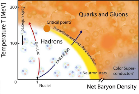
Figure 1.1: Schematic phase diagram of the QCD matter. The net baryon density on x-axis is normalized to that of the normal nuclear matter [gsi.de].

With the advent of modern accelerator facilities, ultra-relativistic heavy-ion collisions have provided an opportunity to systematically create and study different phases of the bulk nuclear matter. It is widely believed that the QGP phase is formed in heavy-ion collision experiments at Relativistic Heavy-Ion Collider (RHIC) located at Brookhaven National Laboratory, USA and Large Hadron Collider (LHC) at European Organization for Nuclear Research (CERN), Geneva. A number of indirect evidences found at the Super Proton Synchrotron (SPS) at CERN, strongly suggested the formation of a “new state of matter” [CERN], but quantitative and clear results were only obtained at RHIC energies [Tannenbaum:2006ch, Kolb, Gyulassy, Tomasik, Muller, Arsene:2004fa, Adcox:2004mh, Back:2004je, Adams:2005dq], and recently at LHC energies [Aamodt:2010pa, Aamodt:2010pb, Aamodt:2010cz, ALICE:2011ab]. The regime with relatively large baryon chemical potential will be probed by the upcoming experimental facilities like Facility for Anti-proton and Ion Research (FAIR) at GSI, Darmstadt. An illustration of the QCD phase diagram and the regions probed by these experimental facilities is shown in Fig. 1.1 [gsi.de].

It is possible to create hot and dense nuclear matter with very high energy densities in relatively large volumes by colliding ultra-relativistic heavy ions. In these conditions, the nuclear matter created may be close to (local) thermodynamic equilibrium, providing the opportunity to investigate the various phases and the thermodynamic and transport properties of QCD. It is important to note that, even though it appears that a deconfined state of matter is formed in these colliders, investigating and extracting the transport properties of QGP from heavy-ion collisions is not an easy task since it cannot be observed directly. Experimentally, it is only feasible to measure energy and momenta of the particles produced in the final stages of the collision, when nuclear matter is already relatively cold and non-interacting. Hence, in order to study the thermodynamic and transport properties of the QGP, the whole heavy ion collision process from the very beginning till the end has to be modelled: starting from the stage where two highly Lorentz contracted heavy nuclei collide with each other, the formation and thermalization of the QGP or de-confined phase in the initial stages of the collision, its subsequent space-time evolution, the phase transition to the hadronic or confined phase of matter, and eventually, the dynamics of the cold hadronic matter formed in the final stages of the collision. The different stages of ultra-relativistic heavy ion collisions are schematically illustrated in Fig. 1.2 [duke.edu].

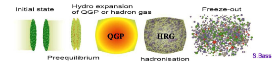
Figure 1.2: Various stages of ultra-relativistic heavy ion collisions [duke.edu].

Assuming that thermalization is achieved in the early stages of heavy-ion collisions and that the interaction between the quarks is strong enough to maintain local thermodynamic equilibrium during the subsequent expansion, the time evolution of the QGP and hadronic matter can be described by the laws of fluid dynamics [Stoecker:1986ci, Rischke:1995ir, Rischke:1995mt, Shuryak:2003xe]. Fluid dynamics, also loosely referred to as hydrodynamics, is an effective approach through which a system can be described by macroscopic variables, such as local energy density, pressure, temperature and flow velocity. Application of viscous hydrodynamics to high-energy heavy-ion collisions has evoked widespread interest ever since a surprisingly small value for the shear viscosity to entropy density ratio $\eta/s$ was estimated from the analysis of the elliptic flow data [Romatschke:2007mq]. Indeed the estimated $\eta/s$ was close to the conjectured lower bound $\eta/s|_{\rm KSS}=1/4\pi$ from ADS/CFT[Policastro:2001yc, Kovtun:2004de]. This led to the claim that the QGP formed at RHIC was the most perfect fluid ever observed. A precise estimate of $\eta/s$ is vital to the understanding of the properties of the QCD matter and is presently a topic of intense investigation, see [Chaudhuri] and references therein.

1.1 Relativistic fluid dynamics

The physical characterization of a system consisting of many degrees of freedom is in general a non-trivial task. For instance, the mathematical formulation of a theory describing the microscopic dynamics of a system containing a large number of interacting particles is one of the most challenging problems of theoretical physics. However, it is possible to provide an effective macroscopic description, over large distance and time scales, by taking into account only the degrees of freedom that are relevant at these scales. This is a consequence of the fact that on macroscopic distance and time scales the actual degrees of freedom of the microscopic theory are imperceptible. Most of the microscopic variables fluctuate rapidly in space and time, hence only average quantities resulting from the interactions at the microscopic level can be observed on macroscopic scales. These rapid fluctuations lead to very small changes of the average values, and hence are not expected to contribute to the macroscopic dynamics. On the other hand, variables that do vary slowly, such as the conserved quantities, are expected to play an important role in the effective description of the system. Fluid dynamics is one of the most common examples of such a situation. It is an effective theory describing the long-wavelength, low frequency limit of the underlying microscopic dynamics of a system.

A fluid is defined as a continuous system in which every infinitesimal volume element is assumed to be close to thermodynamic equilibrium and to remain near equilibrium throughout its evolution. Hence, in other words, in the neighbourhood of each point in space, an infinitesimal volume called fluid element is defined in which the matter is assumed to be homogeneous, i.e., any spatial gradients can be ignored, and is described by a finite number of thermodynamic variables. This implies that each fluid element must be large enough, compared to the microscopic distance scales, to guarantee the proximity to thermodynamic equilibrium, and, at the same time, must be small enough, relative to the macroscopic distance scales, to ensure the continuum limit. The co-existence of both continuous (zero volume) and thermodynamic (infinite volume) limits within a fluid volume might seem paradoxical at first glance. However, if the microscopic and the macroscopic length scales of the system are sufficiently far apart, it is always possible to establish the existence of a volume that is small enough compared to the macroscopic scales, and at the same time, large enough compared to the microscopic ones. In this thesis, we will assume the existence of a clear separation between microscopic and macroscopic scales to guarantee the proximity to local thermodynamic equilibrium.

Relativistic fluid dynamics has been quite successful in explaining the various collective phenomena observed in astrophysics, cosmology and the physics of high-energy heavy-ion collisions. In cosmology and certain areas of astrophysics, one needs a fluid dynamics formulation consistent with the General Theory of Relativity [Ibanez]. On the other hand, a formulation based on the Special Theory of Relativity is quite adequate to treat the evolution of the strongly interacting matter formed in high-energy heavy-ion collisions when it is close to a local thermodynamic equilibrium. In fluid dynamical approach, although no detailed knowledge of the microscopic dynamics is needed, however, knowledge of the equation of state relating pressure, energy density and baryon density is required. The collective behaviour of the hot and dense quark-gluon plasma created in ultra-relativistic heavy-ion collisions has been studied quite extensively within the framework of relativistic fluid dynamics. In application of fluid dynamics, it is natural to first employ the simplest version which is ideal hydrodynamics [26, 27] which neglects the viscous effects and assumes that local equilibrium is always perfectly maintained during the fireball expansion. Microscopically, this requires that the microscopic scattering time be much shorter than the macroscopic expansion (evolution) time. In other words, ideal hydrodynamics assumes that the mean free path of the constituent particles is much smaller than the system size. However, as all fluids are dissipative in nature due to the quantum mechanical uncertainty principle [Danielewicz:1984ww], the ideal fluid results serve only as a benchmark when dissipative effects become important.

When discussing the application of relativistic dissipative fluid dynamics to heavy-ion collision, one is faced with yet another predicament: the theory of relativistic dissipative fluid dynamics is not yet conclusively established. In fact, introducing dissipation in relativistic fluids is not at all a trivial task and still remains one of the important topics of research in high-energy physics. Therefore, in order to quantify the transport properties of the QGP from experiment and confirm the claim that it is indeed the most perfect fluid ever created, the theoretical foundations of relativistic dissipative fluid dynamics must be first addressed and clearly understood.

1.2 Problems in relativistic dissipative fluid dynamics

Ideal hydrodynamics assumes that local thermodynamic equilibrium is perfectly maintained and each fluid element is homogeneous, i.e., spatial gradients are absent (zeroth order in gradient expansion). If this is not satisfied, dissipative effects come into play. The earliest theoretical formulations of relativistic dissipative hydrodynamics also known as first-order theories, are due to Eckart [Eckart:1940zz] and Landau-Lifshitz [Landau]. However, these formulations, collectively called relativistic Navier-Stokes (NS) theory, suffer from acausality and numerical instability. The reason for the acausality is that in the gradient expansion the dissipative currents are linearly proportional to gradients of temperature, chemical potential, and velocity, resulting in parabolic equations. Thus, in Navier-Stokes theory the gradients have an instantaneous influence on the dissipative currents. Such instantaneous effects tend to violate causality and cannot be allowed in a covariant setup, leading to the instabilities investigated in Refs. [Hiscock:1983zz, Hiscock:1985zz, Hiscock:1987zz].

The second-order Israel-Stewart (IS) theory [Israel:1979wp], restores causality but may not guarantee stability [Huovinen:2008te]. The acausality problems were solved by introducing a time delay in the creation of the dissipative currents from gradients of the fluid-dynamical variables. In this case, the dissipative quantities become independent dynamical variables obeying equations of motion that describe their relaxation towards their respective Navier-Stokes values. The resulting equations are hyperbolic in nature which preserves causality. Israel-Stewart theory has been widely applied to ultra-relativistic heavy-ion collisions in order to describe the time evolution of the QGP and the subsequent freeze-out process of the hadron resonance gas.

Hydrodynamic analysis of the spectra and azimuthal anisotropy of particles produced in heavy-ion collisions at RHIC [Romatschke:2007mq, Song:2010mg] and recently at LHC [Luzum:2010ag, Qiu:2011hf] suggests that the matter formed in these collisions is strongly-coupled quark-gluon plasma (sQGP). Although IS hydrodynamics has been quite successful in modelling relativistic heavy ion collisions, there are several inconsistencies and approximations in its formulation which prevent proper understanding of the thermodynamic and transport properties of the QGP. The standard derivation of IS equations using the second-law of thermodynamics contains unknown transport coefficients related to relaxation times of the dissipative quantities viz., the bulk viscous pressure, the particle diffusion current and the shear stress tensor [Israel:1979wp]. While IS equations derived from kinetic theory can provide reliable values for the shear relaxation time ($\tau_{\pi}$), the bulk relaxation time ($\tau_{\Pi}$) still remains ambiguous.

Israel and Stewart’s derivation of second-order hydrodynamics from kinetic theory relies on two additional approximations and assumptions:

1. Grad’s 14-moment approximation: For small departures from equilibrium, the single-particle distribution function is obtained by using a truncated expansion in a Taylor-like series in powers of particle four-momenta $p^{\mu}$ [Israel:1979wp, Grad]. This approximation contains fourteen dynamic variables hence the name 14-moment approximation. Here it is implicitly assumed that the power series in momenta is convergent and is truncated at quadratic order.

2. Choice of second moment of the Boltzmann equation: In a theory with conserved charges the integral over momenta (or zeroth moment) of the Boltzmann equation (BE) leads to conservation of charge current. The first moment of the BE, i.e., momentum integral of the BE weighted with $p^{\mu}$, gives the conservation of the energy-momentum tensor. The derivation of second-order fluid dynamics from kinetic theory by Israel and Stewart is based on the assumption that the second moment of BE must contain information about the non-equilibrium (or dissipative) dynamics of the system [Israel:1979wp, Baier:2006um]. This choice is arbitrary in the sense that higher moments of BE combined with the 14-moment approximation lead to different evolution equations for the dissipative quantities.

Apart from these problems in the formulation, IS theory suffers from several other shortcomings. In one-dimensional Bjorken scaling expansion [Bjorken:1982qr], IS theory leads to negative longitudinal pressure [Martinez:2009mf, Rajagopal:2009yw] which limits its application within a certain temperature range. Further, the scaling solutions of IS equations when compared with transport results show disagreement for shear viscosity to entropy density ratio, $\eta/s>0.5$ indicating the breakdown of the second-order theory [Huovinen:2008te, El:2008yy]. Moreover, in the study of identical particle pair-correlations, the experimentally observed $1/\sqrt{m_{T}}$ scaling of the Hanburry Brown-Twiss (HBT) radii ($m_{T}$ being the transverse mass of the hadron pair), which is also predicted by the ideal hydrodynamics, is broken when viscous corrections to the distribution function are included [Teaney:2003kp]. The correct formulation of the relativistic dissipative fluid dynamics is thus far from settled and is currently under intense investigation [Huovinen:2008te, Baier:2006um, El:2008yy, Betz:2008me, El:2009vj, Martinez:2010sc, Denicol:2010xn, Denicol:2012cn, Jaiswal:2014isa].

In this thesis, we report on some major progress we have made in the formulation of relativistic dissipative fluid dynamics within the framework of kinetic theory. The problem pertaining to the bulk pressure relaxation time, $\tau_{\Pi}$, has been solved by considering entropy four-current defined using Boltzmann H-function [Jaiswal:2013fc]. Using this method, hydrodynamic evolution, production of thermal dileptons and subsequent hadronization of the strongly interacting matter have been studied [Bhalerao:2013aha]. An alternate derivation of the dissipative equations, which does not make use of the 14-moment approximation as well as the second moment of BE, has also been presented [Jaiswal:2013npa]. The form of viscous corrections to the distribution function is derived up to second-order in gradients which restores the observed $1/\sqrt{m_{T}}$ scaling of the HBT radii [Bhalerao:2013pza]. Finally, with the motivation to improve the IS theory beyond its present scope, two rigorous investigations have been presented in this thesis: (a) Derivation of a novel third-order evolution equation for shear stress tensor [Jaiswal:2013vta, Jaiswal:2014raa], and (b) Derivation of second-order dissipative equations from the BE where the collision term is modified to include non-local effects [Jaiswal:2012qm, Jaiswal:2012dd, Jaiswal:2013jja].

1.3 Organization of the thesis

The derivation of a relativistic fluid-dynamical theory consistent with causality, which is applicable to the physics of ultra-relativistic heavy-ion collisions, is the main purpose of this thesis. This thesis is organized in the following manner:

In Chapter 2, we review relativistic fluid dynamics from a phenomenological perspective. We start by deriving the equations of motion of an ideal relativistic fluid and introduce dissipation in a phenomenological manner. Next, the equations of relativistic Navier-Stokes theory are derived via the second law of thermodynamics, and then subsequently extended to Israel-Stewart theory. Then we briefly discuss relativistic kinetic theory and express various hydrodynamic quantities in terms of single-particle, phase-space distribution function. Finally, this chapter concludes with a discussion about the evolution of the phase-space distribution function via Boltzmann equation.

In Chapter 3, we present a derivation of relativistic dissipative hydrodynamic equations, which invokes the second law of thermodynamics for the entropy four-current expressed in terms of the single-particle phase-space distribution function obtained from Grad’s 14-moment approximation. In this derivation all the second-order transport coefficients are uniquely determined within a single theoretical framework. In particular, this removes the long-standing ambiguity in the relaxation time for bulk viscous pressure. We find that in the one-dimensional scaling expansion, these transport coefficients prevent the occurrence of cavitation (negative pressure) even for rather large values of the bulk viscosity estimated in lattice QCD.

In Chapter 4, using the derivation methodology of Chapter 3, we derive relativistic viscous hydrodynamic equations for two different forms of the non-equilibrium single-particle distribution function. These equations are used to study thermal dilepton and hadron spectra within longitudinal scaling expansion of the matter formed in relativistic heavy-ion collisions. We observe that an inconsistent treatment of the nonequilibrium effects influences the particle production significantly.

In Chapter 5, starting from the Boltzmann equation with the relaxation-time approximation for the collision term and using Chapman-Enskog like expansion for distribution function close to equilibrium, we derive hydrodynamic evolution equations for the dissipative quantities directly from their definitions. This derivation does not make use of the two major approximations/assumptions namely, Grad’s 14-moment approximation and second moment of BE, inherent in IS theory. In the case of one-dimensional scaling expansion, we demonstrate that our results are in better agreement with numerical solution of Boltzmann equation as compared to Israel-Stewart results and also show that including approximate higher-order corrections in viscous evolution significantly improves this agreement.

In Chapter 6, we derive the form of viscous corrections to the distribution function up to second-order in gradients by employing iterative solution of Boltzmann equation in relaxation time approximation. Within one dimensional scaling expansion, we demonstrate that while Grad’s 14-moment approximation leads to the violation of the observed $1/\sqrt{m_{T}}$ scaling of HBT radii, the viscous corrections obtained here does not exhibit such unphysical behaviour.

In Chapter 7, we present the derivation of a novel third-order hydrodynamic evolution equation for shear stress tensor from kinetic theory. We quantify the significance of the new derivation within one-dimensional scaling expansion and demonstrate that the results obtained using third-order viscous equations derived here provide a very good approximation to the exact solution of Boltzmann equation in relaxation time approximation. We also show that our results are in better agreement with transport results when compared with an existing third-order calculation based on the second-law of thermodynamics.

In Chapter 8, starting with the relativistic Boltzmann equation where the collision term is generalized to include nonlocal effects via gradients of the phase-space distribution function, and using Grad’s 14-moment approximation for the distribution function, we derive equations for the relativistic dissipative fluid dynamics. This method generates all the second-order terms that are allowed by symmetry, some of which have been missed by the traditional approaches based on the 14-moment approximation. We find that nonlocality of the collision term has a rather strong influence on the evolution of the viscous medium via hydrodynamic equations.

Finally, in Chapter 9 we summarize our results and also discuss the future perspectives for further studies.

1.4 Conventions and notations used

In this thesis, unless stated otherwise, all physical quantities are expressed in terms of natural units, where, $\hbar=c=k_{\rm B}=1$, with $\hbar=h/2\pi$ where $h$ is the Planck constant, $c$ the velocity of light, and $k_{\rm B}$ the Boltzmann constant. Unless stated otherwise, the spacetime is always taken to be Minkowskian where the metric tensor is given by $g_{\mu\nu}=\mbox{diag}(+1,-1,-1,-1)$. Apart from Minkowskian coordinates $x^{\mu}=(t,x,y,z)$, we will also regularly employ Milne coordinate system $x^{\mu}=(\tau,x,y,\eta_{s})$ or $x^{\mu}=(\tau,r,\varphi,\eta_{s})$, with proper time $\tau=\sqrt{t^{2}-z^{2}}$, the radial coordinate $r=\sqrt{x^{2}+y^{2}}$, the azimuthal angle $\varphi=\tan^{-1}(y/x)$, and spacetime rapidity $\eta_{s}=\tanh^{-1}(z/t)$. Hence, $t=\tau\cosh\eta_{s}$, $x=r\cos\varphi$, $y=r\sin\varphi$, and $z=\tau\sinh\eta_{s}$. For the coordinate system $x^{\mu}=(\tau,x,y,\eta_{s})$, the metric becomes $g_{\mu\nu}=\mbox{diag}(1,-1,-1,-\tau^{2})$, whereas for $x^{\mu}=(\tau,r,\varphi,\eta_{s})$, the metric is $g_{\mu\nu}=\mbox{diag}(1,-1,-r^{2},-\tau^{2})$.

Roman letters are used to indicate indices that vary from 1-3 and Greek letters for indices that vary from 0-3. Covariant and contravariant four-vectors are denoted as $p_{\mu}$ and $p^{\mu}$, respectively. The notation $p\cdot q\equiv p_{\mu}q^{\mu}$ represents scalar product of a covariant and a contravariant four-vector. Tensors without indices shall always correspond to Lorentz scalars. We follow Einstein summation convention, which states that repeated indices in a single term are implicitly summed over all the values of that index.

We denote the fluid four-velocity by $u^{\mu}$ and the Lorentz contraction factor by $\gamma$. The projector onto the space orthogonal to $u^{\mu}$ is defined as: $\Delta^{\mu\nu}\equiv g^{\mu\nu}-u^{\mu}u^{\nu}$. Hence, $\Delta^{\mu\nu}$ satisfies the conditions $\Delta^{\mu\nu}u_{\mu}=\Delta^{\mu\nu}u_{\nu}=0$ with trace $\Delta^{\mu}_{\mu}=3$. The partial derivative $\partial^{\mu}$ can then be decomposed as:

$$\partial^{\mu}=\nabla^{\mu}+u^{\mu}D,\quad\mathrm{where~{}}\quad\nabla^{\mu}\equiv\Delta^{\mu\nu}\partial_{\nu}\quad\mathrm{and}\quad D\equiv u^{\mu}\partial_{\mu}.$$

In the fluid rest frame, $D$ reduces to the time derivative and $\nabla^{\mu}$ reduces to the spacial gradient. Hence, the notation $\dot{f}\equiv Df$ is also commonly used. We also frequently use the symmetric, anti-symmetric and angular brackets notations defined as

$$A_{(\mu}B_{\nu)} \equiv \frac{1}{2}\left(A_{\mu}B_{\nu}+A_{\nu}B_{\mu}\right),$$

$$A_{[\mu}B_{\nu]} \equiv \frac{1}{2}\left(A_{\mu}B_{\nu}-A_{\nu}B_{\mu}\right),$$

$$A_{\langle\mu}B_{\nu\rangle} \equiv \Delta^{\alpha\beta}_{\mu\nu}A_{\alpha}B_{\beta}.$$

where,

$$\Delta^{\alpha\beta}_{\mu\nu}\equiv\frac{1}{2}\left(\Delta^{\alpha}_{\mu}\Delta^{\beta}_{\nu}+\Delta^{\alpha}_{\nu}\Delta^{\beta}_{\mu}-\frac{2}{3}\Delta^{\alpha\beta}\Delta_{\mu\nu}\right)$$

is the traceless symmetric projection operator orthogonal to $u^{\mu}$ satisfying the conditions $\Delta^{\alpha\beta}_{\mu\nu}\Delta_{\alpha\beta}=\Delta^{\alpha\beta}_{\mu\nu}\Delta^{\mu\nu}=0$.

Using the above notations, the commonly used local fluid rest frame variables in dissipative viscous hydrodynamics are expressed in terms of the energy momentum tensor $T^{\mu\nu}$, charge four-current $N^{\mu}$ and entropy four-current $S^{\mu}$ as follows:

$$n \equiv \makebox[108.405pt][l]{$u_{\mu}N^{\mu}$}\mbox{net charge density};\hskip 85.35826pt$$

$$n^{\mu} \equiv \makebox[108.405pt][l]{$\bigtriangleup^{\mu}_{\nu}N^{\nu}$}\mbox{net flow of charge};$$

$$\varepsilon \equiv \makebox[108.405pt][l]{$u_{\mu}T^{\mu\nu}u_{\nu}$}\mbox{energy density};$$

$$P+\Pi \equiv -1/3\bigtriangleup_{\mu\nu}T^{\mu\nu} \Pi$$ P: thermal pressure, : bulk pressure;

$$h \equiv (\epsilon+P)/n$$ enthalpy;

$$\pi^{\mu\nu} \equiv \makebox[108.405pt][l]{$T^{\langle\mu\nu\rangle}$ }\mbox{shear stress tensor};$$

$$h^{\mu} \equiv \makebox[108.405pt][l]{$u_{\nu}T^{\nu\lambda}\bigtriangleup^{\mu}_{\lambda}$}\mbox{energy flow};$$

$$q^{\mu} \equiv \makebox[108.405pt][l]{$h^{\mu}-h\,n^{\mu}$}\mbox{heat flow};$$

$$s \equiv \makebox[108.405pt][l]{$u_{\mu}\,S^{\mu}$}\mbox{entropy density};$$

$$\Phi^{\mu} \equiv \makebox[108.405pt][l]{$\bigtriangleup^{\mu}_{\nu}S^{\nu}$}\mbox{entropy flux};$$

$$c_{s}^{2} \equiv \makebox[108.405pt][l]{$(dP/d\epsilon)_{s/n}$}\mbox{adiabatic speed of sound squared}.$$

We also define the following scalar and tensors constructed from the gradients of the fluid four-velocity $u^{\mu}$:

$$\theta \equiv \makebox[216.81pt][l]{$\partial\cdot u$}\mbox{expansion rate},$$

$$\sigma^{\mu\nu} \equiv \makebox[216.81pt][l]{$\nabla^{\langle\mu}u^{\nu\rangle}=\frac{1}{2}(\nabla^{\mu}u^{\nu}+\nabla^{\nu}u^{\mu})-\frac{1}{3}\nabla^{\mu\nu}\partial_{\alpha}u^{\alpha}$}\mbox{velocity stress tensor},$$

$$\omega^{\mu\nu} \equiv \makebox[216.81pt][l]{$\nabla^{[\mu}u^{\nu]}$}\mbox{vorticity tensor}.$$

Chapter 2 Thermodynamics, relativistic fluid dynamics and kinetic theory

The most appealing feature of relativistic fluid dynamics is the fact that it is simple and general. It is simple in the sense that all the information of the system is contained in its thermodynamic and transport properties, i.e., its equation of state and transport coefficients. Fluid dynamics is also general because it relies on only one assumption: the system remains close to local thermodynamic equilibrium throughout its evolution. Although the hypothesis of proximity to local equilibrium is quite strong, it saves us from making any further assumption regarding the description of the particles and fields, their interactions, the classical or quantum nature of the phenomena involved etc. In this chapter, we review the basic aspects of thermodynamics and discuss relativistic fluid dynamics from a phenomenological perspective. The salient features of kinetic theory in the context of fluid dynamics will also be discussed. The concepts introduced in this Chapter will be required in the following Chapters to derive dissipative hydrodynamic equations for applications in high-energy heavy-ion physics.

This chapter is organized as follows: In Sec. 2.1, we introduce the basic laws of thermodynamics and derive the thermodynamic relations that will be used later in this thesis. Section 2.2 contains a brief review of relativistic ideal fluid dynamics. We derive the general form of the conserved currents of an ideal fluid and their equations of motion. In Sec. 2.3, we postulate the thermodynamic relations in a covariant notation using the definition of hydrodynamic four-velocity from the previous section. In Sec. 2.4 we introduce dissipation in fluid dynamics, explain the basic aspects of dissipative fluid dynamics and derive a covariant version of Navier-Stokes theory using the second law of thermodynamics. We discuss the problems of Navier-Stokes theory in the relativistic regime, i.e., the acausality and instability of this theory. We also review Israel-Stewart theory and show how to derive causal fluid dynamical equations from the second law of thermodynamics. Finally, Sec. 2.5 contains a discussion about the relativistic kinetic theory, where we express fluid dynamical currents in terms of single-particle phase-space distribution function. We also outline the basic aspects of relativistic Boltzmann equation and its implications on the evolution of the distribution function.

2.1 Thermodynamics

Thermodynamics is an empirical description of the macroscopic or large-scale properties of matter and it makes no hypotheses about the small-scale or microscopic structure. It is concerned only with the average behaviour of a very large number of microscopic constituents, and its laws can be derived from statistical mechanics. A thermodynamic system can be described in terms of a small set of extensive variables, such as volume ($V$), the total energy ($E$), entropy ($S$), and number of particles ($N$), of the system. Thermodynamics is based on four phenomenological laws that explain how these quantities are related and how they change with time [Fermi, Reif, Reichl].

• Zeroth Law: If two systems are both in thermal equilibrium with a third system then they are in thermal equilibrium with each other. This law helps define the notion of temperature.

• First Law: All the energy transfers must be accounted for to ensure the conservation of the total energy of a thermodynamic system and its surroundings. This law is the principle of conservation of energy.

• Second Law: An isolated physical system spontaneously evolves towards its own internal state of thermodynamic equilibrium. Employing the notion of entropy, this law states that the change in entropy of a closed thermodynamic system is always positive or zero.

• Third Law: Also known an Nernst’s heat theorem, states that the difference in entropy between systems connected by a reversible process is zero in the limit of vanishing temperature. In other words, it is impossible to reduce the temperature of a system to absolute zero in a finite number of operations.

The first law of thermodynamics postulates that the changes in the total energy of a thermodynamic system must result from: (1) heat exchange, (2) the mechanical work done by an external force, and (3) from particle exchange with an external medium. Hence the conservation law relating the small changes in state variables, $E$, $V$, and $N$ is

$$\delta E=\delta Q-P\delta V+\mu\,\delta N,$$ (2.1)

where $P$ and $\mu$ are the pressure and chemical potential, respectively, and $\delta Q$ is the amount of heat exchange.

The heat exchange takes into account the energy variations due to changes of internal degrees of freedom that are not described by the state variables. The heat itself is not a state variable since it can depend on the past evolution of the system and may take several values for the same thermodynamic state. However, when dealing with reversible processes (in time), it becomes possible to assign a state variable related to heat. This variable is the entropy, $S$ , and is defined in terms of the heat exchange as $\delta Q=T\delta S$, with the temperature $T$ being the proportionality constant. Then, when considering variations between equilibrium states that are infinitesimally close to each other, it is possible to write the first law of thermodynamics in terms of differentials of the state variables,

$$dE=TdS-PdV+\mu\,dN.$$ (2.2)

Hence, using Eq. (2.2), the intensive quantities, $T$, $\mu$ and $P$, can be obtained in terms of partial derivatives of the entropy as

$$\left.{\frac{\partial S}{\partial E}}\right|_{N,V}=\frac{1}{T},\qquad\left.{\frac{\partial S}{\partial V}}\right|_{N,E}=\frac{P}{T},\qquad\left.{\frac{\partial S}{\partial N}}\right|_{E,V}=-\frac{\mu}{T}.$$ (2.3)

The entropy is mathematically defined as an extensive and additive function of the state variables, which means that

$$S(\lambda E,\lambda V,\lambda N)=\lambda S(E,V,N).$$ (2.4)

Differentiating both sides with respect to $\lambda$, we obtain

$$S=E\left.{\frac{\partial S}{\partial\lambda E}}\right|_{\lambda N,\lambda V}+V\left.{\frac{\partial S}{\partial\lambda V}}\right|_{\lambda N,\lambda E}+N\left.{\frac{\partial S}{\partial\lambda N}}\right|_{\lambda E,\lambda V},$$ (2.5)

which holds for any arbitrary value of $\lambda$. Setting $\lambda=1$ and using Eq. (2.3), we obtain the so-called Euler’s relation

$$E=-PV+TS+\mu\,N.$$ (2.6)

Using Euler’s relation, Eq. (2.6), along with the first law of thermodynamics, Eq. (2.2), we arrive at the Gibbs-Duhem relation

$$VdP=SdT+Nd\mu.$$ (2.7)

In terms of energy, entropy and number densities defined as $\epsilon\equiv E/V$, $s\equiv S/V$, and $n\equiv N/V$ respectively, the Euler’s relation, Eq. (2.6) and Gibbs-Duhem relation, Eq. (2.7), reduce to

$$\epsilon =-P+Ts+\mu\,n$$ (2.8)

$$dP =s\,dT+n\,d\mu.$$ (2.9)

Differentiating Eq.(2.8) and using Eq. (2.9), we obtain the relation analogous to first law of thermodynamics

$$d\epsilon=Tds+\mu\,dn\quad\Rightarrow\quad ds=\frac{1}{T}\,d\epsilon-\frac{\mu}{T}\,dn.$$ (2.10)

It is important to note that all the densities defined above $(\epsilon,~{}s,~{}n)$ are intensive quantities.

The equilibrium state of a system is defined as a stationary state where the extensive and intensive variables of the system do not change. We know from the second law of thermodynamics that the entropy of an isolated thermodynamic system must either increase or remain constant. Hence, if a thermodynamic system is in equilibrium, the entropy of the system being an extensive variable, must remain constant. On the other hand, for a system that is out of equilibrium, the entropy must always increase. This is an extremely powerful concept that will be extensively used in this chapter to constrain and derive the equations of motion of a dissipative fluid. This concludes a brief outline of the basics of thermodynamics; for a more detailed review, see Ref. [Reichl]. In the next section, we introduce and derive the equations of relativistic ideal fluid dynamics.

2.2 Relativistic ideal fluid dynamics

An ideal fluid is defined by the assumption of local thermal equilibrium, i.e., all fluid elements must be exactly in thermodynamic equilibrium [Landau, Weinberg]. This means that at each space-time coordinate of the fluid $x\equiv x^{\mu}$, there can be assigned a temperature $T(x)$, a chemical potential $\mu(x)$, and a collective four-velocity field,

$$u^{\mu}(x)\equiv\frac{dx^{\mu}}{d\tau}.$$ (2.11)

The proper time increment $d\tau$ is given by the line element

$$(d\tau)^{2}=g_{\mu\nu}dx^{\mu}dx^{\nu}=(dt)^{2}-(d\vec{x})^{2}=(dt)^{2}\left[1-(\vec{v})^{2}\right],$$ (2.12)

where $\vec{v}\equiv d\vec{x}/dt$. This implies that

$$u^{\mu}(x)=\frac{dt}{d\tau}\frac{dx^{\mu}}{dt}=\gamma(\vec{v})\binom{1}{\vec{v}}$$ (2.13)

where $\gamma(\vec{v})=1/\sqrt{1-\vec{v}^{2}}$. In the non-relativistic limit, we obtain $u^{\mu}(x)=(1,\vec{v})$. It is important to note that the four-vector $u^{\mu}(x)$ only contains three independent components since it obeys the relation

$$u^{2}\equiv u^{\mu}(x)g_{\mu\nu}u^{\nu}(x)=\gamma^{2}(\vec{v})\left(1-\vec{v}^{2}\right)=1.$$ (2.14)

The quantities $T$, $\mu$ and $u^{\mu}$ are often referred to as the primary fluid-dynamical variables.

The state of a fluid can be completely specified by the densities and currents associated with conserved quantities, i.e., energy, momentum, and (net) particle number. For a relativistic fluid, the state variables are the energy- momentum tensor, $T^{\mu\nu}$, and the (net) particle four-current, $N^{\mu}$. To obtain the general form of these currents for an ideal fluid, we first define the local rest frame (LRF) of the fluid. In this frame, $\vec{v}=0$, and the energy-momentum tensor, $T^{\mu\nu}_{LRF}$, the (net) particle four-current, $N^{\mu}_{LRF}$, and the entropy four-current, $S^{\mu}_{LRF}$, should have the characteristic form of a system in static equilibrium. In other words, in local rest frame, there is no flow of energy ($T^{i0}_{LRF}=0$), the force per unit surface element is isotropic ($T^{ij}_{LRF}=\delta^{ij}P$) and there is no particle and entropy flow ($\vec{N}=0$ and $\vec{S}=0$). Consequently, the energy-momentum tensor, particle and entropy four-currents in this frame take the following simple forms

$$T^{\mu\nu}_{LRF}=\left(\begin{array}[]{cccc}\epsilon&0&0&0\\ 0&P&0&0\\ 0&0&P&0\\ 0&0&0&P\end{array}\right)\!,\quad N^{\mu}_{LRF}=\left(\begin{array}[]{c}n\\ 0\\ 0\\ 0\end{array}\right)\!,\quad S^{\mu}_{LRF}=\left(\begin{array}[]{c}s\\ 0\\ 0\\ 0\end{array}\right)\!.$$ (2.15)

For an ideal relativistic fluid, the general form of the energy-momentum tensor, $T^{\mu\nu}_{(0)}$, (net) particle four-current, $N^{\mu}_{(0)}$, and the entropy four-current, $S^{\mu}_{(0)}$, has to be built out of the hydrodynamic tensor degrees of freedom, namely the vector, $u^{\mu}$, and the metric tensor, $g_{\mu\nu}$. Since $T^{\mu\nu}_{(0)}$ should be symmetric and transform as a tensor, and, $N^{\mu}_{(0)}$ and $S^{\mu}_{(0)}$ should transform as a vector, under Lorentz transformations, the most general form allowed is therefore

$$T^{\mu\nu}_{(0)}=c_{1}u^{\mu}u^{\nu}+c_{2}g^{\mu\nu},\quad N^{\mu}_{(0)}=c_{3}u^{\mu},\quad S^{\mu}_{(0)}=c_{4}u^{\mu}.$$ (2.16)

In the local rest frame, $\vec{v}=0\Rightarrow u^{\mu}=(1,\vec{0})$. Hence in this frame, Eq. (2.16) takes the form

$$T^{\mu\nu}_{(0)LRF}=\left(\begin{array}[]{cccc}c_{1}+c_{2}&0&0&0\\ 0&-c_{2}&0&0\\ 0&0&-c_{2}&0\\ 0&0&0&-c_{2}\end{array}\right)\!\!,\quad N^{\mu}_{(0)LRF}=\left(\begin{array}[]{c}c_{3}\\ 0\\ 0\\ 0\end{array}\right)\!\!,\quad S^{\mu}_{(0)LRF}=\left(\begin{array}[]{c}c_{4}\\ 0\\ 0\\ 0\end{array}\right)\!\!.$$ (2.17)

By comparing the above equation with the corresponding general expressions in the local rest frame, Eq. (2.15), one obtains the following expressions for the coefficients

$$c_{1}=\epsilon+P,\quad c_{2}=-P,\quad c_{3}=n,\quad c_{4}=s.$$ (2.18)

The conserved currents of an ideal fluid can then be expressed as

$$T^{\mu\nu}_{(0)}=\epsilon u^{\mu}u^{\nu}-P\Delta^{\mu\nu},\quad N^{\mu}_{(0)}=nu^{\mu},\quad S^{\mu}_{(0)}=su^{\mu},$$ (2.19)

where $\Delta^{\mu\nu}=g^{\mu\nu}-u^{\mu}u^{\nu}$ is the projection operator onto the three-space orthogonal to $u^{\mu}$, and satisfies the following properties of an orthogonal projector,

$$u_{\mu}\Delta^{\mu\nu}=\Delta^{\mu\nu}u_{\nu}=0,\quad\Delta^{\mu}_{\rho}\Delta^{\rho\nu}=\Delta^{\mu\nu},\quad\Delta^{\mu}_{\mu}=3.$$ (2.20)

The dynamical description of an ideal fluid is obtained using the conservation laws of energy, momentum and (net) particle number. These conservation laws can be mathematically expressed using the four-divergences of energy-momentum tensor and particle four-current which leads to the following equations,

$$\partial_{\mu}T^{\mu\nu}_{(0)}=0,\quad\partial_{\mu}N^{\mu}_{(0)}=0,$$ (2.21)

where the partial derivative $\partial_{\mu}\equiv\partial/\partial x^{\mu}$ transforms as a covariant vector under Lorentz transformations. Using the four-velocity, $u^{\mu}$, and the projection operator, $\Delta^{\mu\nu}$, the derivative, $\partial_{\mu}$, can be projected along and orthogonal to $u^{\mu}$

$$D\equiv u^{\mu}\partial_{\mu},\quad\nabla_{\mu}\equiv\Delta_{\mu}^{\rho}\partial_{\rho},\quad\Rightarrow\quad\partial_{\mu}=u_{\mu}D+\nabla_{\mu}.$$ (2.22)

Projection of energy-momentum conservation equation along and orthogonal to $u^{\mu}$ together with the conservation law for particle number, leads to the equations of motion of ideal fluid dynamics,

$$u_{\mu}\partial_{\nu}T^{\mu\nu}_{(0)}=0 \quad\Rightarrow\quad D\epsilon+(\epsilon+P)\theta=0,$$ (2.23)

$$\Delta^{\alpha}_{\mu}\partial_{\nu}T^{\mu\nu}_{(0)}=0 \quad\Rightarrow\quad(\epsilon+P)Du^{\alpha}-\nabla^{\alpha}P=0,$$ (2.24)

$$\partial_{\mu}N^{\mu}_{(0)}=0 \quad\Rightarrow\quad Dn+n\theta=0,$$ (2.25)

where $\theta\equiv\partial_{\mu}u^{\mu}$. It is important to note that an ideal fluid is described by four fields, $\epsilon$, $P$, $n$, and $u_{\mu}$, corresponding to six independent degrees of freedom. The conservation laws, on the other hand, provide only five equations of motion. The equation of state of the fluid, $P=P(n,\epsilon)$, relating the pressure to other thermodynamic variables has to be specified to close this system of equations. The existence of equation of state is guaranteed by the assumption of local thermal equilibrium and hence the equations of ideal fluid dynamics are always closed.

2.3 Covariant thermodynamics

In the following, we re-write the equilibrium thermodynamic relations derived in Sec. 2.1, Eqs. (2.8), (2.9), and (2.10), in a covariant form [Israel:1979wp, Israel:1976tn]. For this purpose, it is convenient to introduce the following notations

$$\beta\equiv\frac{1}{T},\quad\alpha\equiv\frac{\mu}{T},\quad\beta^{\mu}\equiv\frac{u^{\mu}}{T}.$$ (2.26)

In these notations, the covariant version of the Euler’s relation, Eq. (2.8), and the Gibbs-Duhem relation, Eq. (2.9), can be postulated as,

$$S^{\mu}_{(0)} =P\beta^{\mu}+\beta_{\nu}T^{\mu\nu}_{(0)}-\alpha N^{\mu}_{(0)},$$ (2.27)

$$d\left(P\beta^{\mu}\right) =N^{\mu}_{(0)}d\alpha-T^{\mu\nu}_{(0)}d\beta_{\nu},$$ (2.28)

respectively. The above equations can then be used to derive a covariant form of the first law of thermodynamics, Eq. (2.10),

$$dS^{\mu}_{(0)}=\beta_{\nu}dT^{\mu\nu}_{(0)}-\alpha dN^{\mu}_{(0)}.$$ (2.29)

The covariant thermodynamic relations were constructed in a such a way that when Eqs. (2.27), (2.28) and (2.29) are contracted with $u_{\mu}$,

$$u_{\mu}\left[S^{\mu}_{(0)}-P\beta^{\mu}-\beta_{\nu}T^{\mu\nu}_{(0)}+\alpha N^{\mu}_{(0)}\right] =0\quad\Rightarrow\quad s+\alpha n-\beta(\epsilon+P)=0,$$ (2.30)

$$u_{\mu}\left[d\left(P\beta^{\mu}\right)-N^{\mu}_{(0)}d\alpha+T^{\mu\nu}_{(0)}d\beta_{\nu}\right] =0\quad\Rightarrow\quad d(\beta P)-nd\alpha+\epsilon d\beta=0,$$ (2.31)

$$u_{\mu}\left[dS^{\mu}_{(0)}-\beta_{\nu}dT^{\mu\nu}_{(0)}+\alpha dN^{\mu}_{(0)}\right] =0\quad\Rightarrow\quad ds-\beta d\epsilon+\alpha dn=0,$$ (2.32)

we obtain the usual thermodynamic relations, Eqs. (2.8), (2.9), and (2.10). Here we have used the property of the fluid four-velocity, $u_{\mu}u^{\mu}=1\Rightarrow u_{\mu}du^{\mu}=0$. The projection of Eqs. (2.27), (2.28) and (2.29) onto the three-space orthogonal to $u^{\mu}$ just leads to trivial identities,

$$\Delta^{\alpha}_{\mu}\left[S^{\mu}_{(0)}-P\beta^{\mu}-\beta_{\nu}T^{\mu\nu}_{(0)}+\alpha N^{\mu}_{(0)}\right] =0\quad\Rightarrow\quad 0=0,$$ (2.33)

$$\Delta^{\alpha}_{\mu}\left[d\left(P\beta^{\mu}\right)-N^{\mu}_{(0)}d\alpha+T^{\mu\nu}_{(0)}d\beta_{\nu}\right] =0\quad\Rightarrow\quad 0=0,$$ (2.34)

$$\Delta^{\alpha}_{\mu}\left[dS^{\mu}_{(0)}-\beta_{\nu}dT^{\mu\nu}_{(0)}+\alpha dN^{\mu}_{(0)}\right] =0\quad\Rightarrow\quad 0=0.$$ (2.35)

From the above equations we conclude that the covariant thermodynamic relations do not contain more information than the usual thermodynamic relations.

The first law of thermodynamics, Eq. (2.29), leads to the following expression for the entropy four-current divergence,

$$\partial_{\mu}S^{\mu}_{(0)}=\beta_{\mu}\partial_{\nu}T^{\mu\nu}_{(0)}-\alpha\partial_{\mu}N^{\mu}_{(0)}.$$ (2.36)

After employing the conservation of energy-momentum and net particle number, Eq. (2.21), the above equation leads to the conservation of entropy, $\partial_{\mu}S^{\mu}_{(0)}=0$. It is important to note that within equilibrium thermodynamics, the entropy conservation is a natural consequence of energy-momentum and particle number conservation, and the first law of thermodynamics. The equation of motion for the entropy density is then obtained as

$$\partial_{\mu}S^{\mu}_{(0)}=0\quad\Rightarrow\quad Ds+s\theta=0.$$ (2.37)

We observe that the rate equation of the entropy density in the above equation is identical to that of the net particle number, Eq. (2.25). Therefore, we conclude that for ideal hydrodynamics, the ratio of entropy density to number density ($s/n$) is a constant of motion.

2.4 Relativistic dissipative fluid dynamics

The derivation of relativistic ideal fluid dynamics proceeds by employing the properties of the Lorentz transformation, the conservation laws, and most importantly, by imposing local thermodynamic equilibrium. It is important to note that while the properties of Lorentz transformation and the conservation laws are robust, the assumption of local thermodynamic equilibrium is a strong restriction. The deviation from local thermodynamic equilibrium results in dissipative effects, and, as all fluids are dissipative in nature due to the uncertainty principle [Danielewicz:1984ww], the assumption of local thermodynamic equilibrium is never strictly realized in practice. In the following, we consider a more general theory of fluid dynamics that attempts to take into account the dissipative processes that must happen, because a fluid can never maintain exact local thermodynamic equilibrium throughout its dynamical evolution.

Dissipative effects in a fluid originate from irreversible thermodynamic processes that occur during the motion of the fluid. In general, each fluid element may not be in equilibrium with the whole fluid, and, in order to approach equilibrium, it exchanges heat with its surroundings. Moreover, the fluid elements are in relative motion and can also dissipate energy by friction. All these processes must be included in order to obtain a reasonable description of a relativistic fluid.

The earliest covariant formulation of dissipative fluid dynamics were due to Eckart [Eckart:1940zz], in 1940, and, later, by Landau and Lifshitz [Landau], in 1959. The formulation of these theories, collectively known as first-order theories (order of gradients), was based on a covariant generalization of the Navier-Stokes theory. The Navier-Stokes theory, at that time, had already become a successful theory of dissipative fluid dynamics. It was employed efficiently to describe a wide variety of non-relativistic fluids, from weakly coupled gases such as air, to strongly coupled fluids such as water. Hence, a relativistic generalisation of Navier-Stokes theory was considered to be the most effective and promising way to describe relativistic dissipative fluids.

The formulation of relativistic dissipative hydrodynamics turned out to be more subtle since the relativistic generalisation of Navier-Stokes theory is intrinsically unstable [Hiscock:1983zz, Hiscock:1985zz, Hiscock:1987zz]. The source of such instability is attributed to the inherent acausal behaviour of this theory [Denicol:2008ha, Pu:2009fj]. A straightforward relativistic generalisation of Navier-Stokes theory allows signals to propagate with infinite speed in a medium. While in non-relativistic theories, this does not give rise to an intrinsic problem and can be ignored, in relativistic systems where causality is a physical property that is naturally preserved, this feature leads to intrinsically unstable equations of motion. Nevertheless, it is instructive to review the first-order theories as they are an important initial step to illustrate the basic features of relativistic dissipative fluid-dynamics.

As in the case of ideal fluids, the basic equations governing the motion of dissipative fluids are also obtained from the conservation laws of energy-momentum and (net) particle number,

$$\partial_{\mu}T^{\mu\nu}=0,\quad\partial_{\mu}N^{\mu}=0.$$ (2.38)

However, for dissipative fluids, the energy-momentum tensor is no longer diagonal and isotropic in the local rest frame. Moreover, due to diffusion, the particle flow is expected to appear in the local rest frame of the fluid element. To account for these effects, dissipative currents $\tau^{\mu\nu}$ and $n^{\mu}$ are added to the previously derived ideal currents, $T^{\mu\nu}_{(0)}$ and $N^{\mu}_{(0)}$,

$$T^{\mu\nu}=T^{\mu\nu}_{(0)}+\tau^{\mu\nu}=\epsilon u^{\mu}u^{\nu}-P\Delta^{\mu\nu}+\tau^{\mu\nu},\quad N^{\mu}=N^{\mu}_{(0)}+n^{\mu}=nu^{\mu}+n^{\mu},$$ (2.39)

where, $\tau^{\mu\nu}$ is required to be symmetric ($\tau^{\mu\nu}=\tau^{\nu\mu}$) in order to satisfy angular momentum conservation. The main objective then becomes to find the dynamical or constitutive equations satisfied by these dissipative currents.

2.4.1 Matching conditions

The introduction of the dissipative currents causes the equilibrium variables to be ill-defined, since the fluid can no longer be considered to be in local thermodynamic equilibrium. Hence, in a dissipative fluid, the thermodynamic variables can only be defined in terms of an artificial equilibrium state, constructed such that the thermodynamic relations are valid as if the fluid were in local thermodynamic equilibrium. The first step to construct such an equilibrium state is to define $\epsilon$ and $n$ as the total energy and particle density in the local rest frame of the fluid, respectively. This is guaranteed by imposing the so-called matching or fitting conditions [Israel:1979wp],

$$\epsilon\equiv u_{\mu}u_{\nu}T^{\mu\nu},\quad n\equiv u_{\mu}N^{\mu}.$$ (2.40)

These matching conditions enforces the following constraints on the dissipative currents

$$u_{\mu}u_{\nu}\tau^{\mu\nu}=0,\quad u_{\mu}n^{\mu}=0.$$ (2.41)

Subsequently, using $n$ and $\epsilon$, an artificial equilibrium state can be constructed with the help of the equation of state. It is however important to note that while the energy and particle densities are physically defined, all the other thermodynamic quantities ($s,~{}P,~{}T,~{}\mu,\cdots$) are defined only in terms of an artificial equilibrium state and do not necessarily retain their usual physical meaning.

2.4.2 Tensor decompositions of dissipative quantities

To proceed further, it is convenient to decompose $\tau^{\mu\nu}$ in terms of its irreducible components, i.e., a scalar, a four-vector, and a traceless and symmetric second-rank tensor. Moreover, this tensor decomposition must be consistent with the matching or orthogonality condition, Eq. (2.41), satisfied by $\tau^{\mu\nu}$. To this end, we introduce another projection operator, the double symmetric, traceless projector orthogonal to $u^{\mu}$,

$$\Delta^{\mu\nu}_{\alpha\beta}\equiv\frac{1}{2}\left(\Delta^{\mu}_{\alpha}\Delta^{\nu}_{\beta}+\Delta^{\mu}_{\beta}\Delta^{\nu}_{\alpha}-\frac{2}{3}\Delta^{\mu\nu}\Delta_{\alpha\beta}\right),$$ (2.42)

with the following properties,

$$\Delta^{\mu\nu}_{~{}~{}~{}\alpha\beta}=\Delta^{~{}~{}~{}\mu\nu}_{\alpha\beta},\quad\Delta^{\mu\nu}_{\rho\sigma}\Delta^{\rho\sigma}_{\alpha\beta}=\Delta^{\mu\nu}_{\alpha\beta},\quad u_{\mu}\Delta^{\mu\nu}_{\alpha\beta}=g_{\mu\nu}\Delta^{\mu\nu}_{\alpha\beta}=0,\quad\Delta^{\mu\nu}_{\mu\nu}=5.$$ (2.43)

The parentheses in the above equation denote symmetrization of the Lorentz indices, i.e., $A^{(\mu\nu)}\equiv(A^{\mu\nu}+A^{\nu\mu})/2$. The dissipative current $\tau^{\mu\nu}$ then can be tensor decomposed in its irreducible form by using $u^{\mu}$, $\Delta^{\mu\nu}$ and $\Delta^{\mu\nu}_{\alpha\beta}$ as

$$\tau^{\mu\nu}\equiv-\Pi\Delta^{\mu\nu}+2u^{(\mu}h^{\nu)}+\pi^{\mu\nu},$$ (2.44)

where we have defined

$$\Pi\equiv-\frac{1}{3}\Delta_{\alpha\beta}\tau^{\alpha\beta},\quad h^{\mu}\equiv\Delta^{\mu}_{\alpha}u_{\beta}\tau^{\alpha\beta},\quad\pi^{\mu\nu}\equiv\Delta^{\mu\nu}_{\alpha\beta}\tau^{\alpha\beta}.$$ (2.45)

The scalar $\Pi$ is the bulk viscous pressure, the vector $h^{\mu}$ is the energy-diffusion four-current, and the second-rank tensor $\pi^{\mu\nu}$ is the shear-stress tensor. The properties of the projection operators $\Delta^{\mu}_{\alpha}$ and $\Delta^{\mu\nu}_{\alpha\beta}$ imply that both $h^{\mu}$ and $\pi^{\mu\nu}$ are orthogonal to $u^{\mu}$ and, additionally, $\pi^{\mu\nu}$ is traceless. Armed with these definitions, all the irreducible hydrodynamic fields are expressed in terms of $N^{\mu}$ and $T^{\mu\nu}$ as

$$\epsilon =u_{\alpha}u_{\beta}T^{\alpha\beta},\quad n=u_{\alpha}N^{\alpha},\quad\Pi=-P-\frac{1}{3}\Delta_{\alpha\beta}T^{\alpha\beta},$$

$$h^{\mu} =u_{\alpha}T^{\langle\mu\rangle\alpha},\quad n^{\mu}=N^{\langle\mu\rangle},\quad\pi^{\mu\nu}=T^{\langle\mu\nu\rangle},$$ (2.46)

where the angular bracket notations are defined as, $A^{\langle\mu\rangle}\equiv\Delta^{\mu}_{\alpha}A^{\alpha}$ and $B^{\langle\mu\nu\rangle}\equiv\Delta^{\mu\nu}_{\alpha\beta}B^{\alpha\beta}$.

We observe that $T^{\mu\nu}$ is a symmetric second-rank tensor with ten independent components and $N^{\mu}$ is a four-vector; overall they have fourteen independent components. Next we count the number of independent components in the tensor decompositions of $T^{\mu\nu}$ and $N^{\mu}$. Since $n^{\mu}$ and $h^{\mu}$ are orthogonal to $u^{\mu}$, they can have only three independent components each. The shear-stress tensor $\pi^{\mu\nu}$ is symmetric, traceless and orthogonal to $u^{\mu}$, and hence, can have only five independent components. Together with $u^{\mu}$, $\epsilon$, $n$ and $\Pi$, which have in total six independent components ($P$ is related to $\epsilon$ via equation of state), we count a total of seventeen independent components, three more than expected. The reason being that so far, the velocity field $u^{\mu}$ was introduced as a general normalized four-vector and was not specified. Hence $u^{\mu}$ has to be defined to reduce the number of independent components to the correct value.

2.4.3 Definition of the velocity field

In the process of formulating the theory of dissipative fluid dynamics, the next important step is to fix $u^{\mu}$. In the case of ideal fluids, the local rest frame was defined as the frame in which there is, simultaneously, no net energy and particle flow. While the definition of local rest frame was unambiguous for ideal fluids, this definition is no longer possible in the case of dissipative fluids due to the presence of both energy and particle diffusion. From a mathematical perspective, the fluid velocity can be defined in numerous ways. However, from the physical perspective, there are two natural choices. The Eckart definition [Eckart:1940zz], in which the velocity is defined by the flow of particles

$$N^{\mu}=nu^{\mu}\quad\Rightarrow\quad n^{\mu}=0,$$ (2.47)

and the Landau definition [Landau], in which the velocity is specified by the flow of the total energy

$$u_{\nu}T^{\mu\nu}=\epsilon u^{\mu}\quad\Rightarrow\quad h^{\mu}=0.$$ (2.48)

We note that the above two definitions of $u^{\mu}$ impose different constraints on the dissipative currents. In the Eckart definition the particle diffusion is always set to zero, while in the Landau definition, the energy diffusion is zero. In other words, the Eckart definition of the velocity field eliminates any diffusion of particles whereas the Landau definition eliminates any diffusion of energy. In this thesis, we shall always use the Landau definition, Eq. (2.48). The conserved currents in this frame take the following form

$$T^{\mu\nu}=\epsilon u^{\mu}u^{\nu}-(P+\Pi)\Delta^{\mu\nu}+\pi^{\mu\nu},\quad N^{\mu}=nu^{\mu}+n^{\mu}.$$ (2.49)

As done for ideal fluids, the energy-momentum conservation equation in Eq. (2.38) is decomposed parallel and orthogonal to $u^{\mu}$. Using Eq. (2.49) together with the conservation law for particle number in Eq. (2.38), leads to the equations of motion for dissipative fluids,

$$u_{\mu}\partial_{\nu}T^{\mu\nu}=0 \quad\Rightarrow\quad\dot{\epsilon}+(\epsilon+P+\Pi)\theta-\pi^{\mu\nu}\sigma_{\mu\nu}=0,$$ (2.50)

$$\Delta^{\alpha}_{\mu}\partial_{\nu}T^{\mu\nu}=0 \quad\Rightarrow\quad(\epsilon+P+\Pi)\dot{u}^{\alpha}-\nabla^{\alpha}(P+\Pi)+\Delta^{\alpha}_{\mu}\partial_{\nu}\pi^{\mu\nu}=0,$$ (2.51)

$$\partial_{\mu}N^{\mu}=0 \quad\Rightarrow\quad\dot{n}+n\theta+\partial_{\mu}n^{\mu}=0,$$ (2.52)

where $\dot{A}\equiv DA=u^{\mu}\partial_{\mu}A$, and the shear tensor $\sigma^{\mu\nu}\equiv\nabla^{\langle\mu}u^{\nu\rangle}=\Delta^{\mu\nu}_{\alpha\beta}\nabla^{\alpha}u^{\beta}$.

We observe that while there are fourteen total independent components of $T^{\mu\nu}$ and $N^{\mu}$, Eqs. (2.50)-(2.52) constitute only five equations. Therefore, in order to derive the complete set of equations for dissipative fluid dynamics, one still has to obtain the additional nine equations of motion that will close Eqs. (2.50)-(2.52). Eventually, this corresponds to finding the closed dynamical or constitutive relations satisfied by the dissipative tensors $\Pi$, $n^{\mu}$ and $\pi^{\mu\nu}$.

2.4.4 Relativistic Navier-Stokes theory

In the presence of dissipative currents, the entropy is no longer a conserved quantity, i.e., $\partial_{\mu}S^{\mu}\neq 0$. Since the form of the entropy four-current for a dissipative fluid is not known a priori, it is not trivial to obtain its equation. We proceed by recalling the form of the entropy four-current for ideal fluids, Eq. (2.27), and extending it for dissipative fluids,

$$S^{\mu}=P\beta^{\mu}+\beta_{\nu}T^{\mu\nu}-\alpha N^{\mu}.$$ (2.53)

The above extension remains valid because an artificial equilibrium state was constructed using the matching conditions to satisfy the thermodynamic relations as if in equilibrium. This was the key step proposed by Eckart, Landau and Lifshitz in order to derive the relativistic Navier-Stokes theory [Eckart:1940zz, Landau]. The next step is to calculate the entropy generation, $\partial_{\mu}S^{\mu}$, in dissipative fluids. To this end, we substitute the form of $T^{\mu\nu}$ and $N^{\mu}$ for dissipative fluids from Eq. (2.49) in Eq. (2.53). Taking the divergence and using Eqs. (2.50)-(2.52), we obtain

$$\partial_{\mu}S^{\mu}=-\beta\Pi\theta-n^{\mu}\nabla_{\mu}\alpha+\beta\pi^{\mu\nu}\sigma_{\mu\nu}.$$ (2.54)

The relativistic Navier-Stokes theory can then be obtained by applying the second law of thermodynamics to each fluid element, i.e., by requiring that the entropy production $\partial_{\mu}S^{\mu}$ must always be positive,

$$-\beta\Pi\theta-n^{\mu}\nabla_{\mu}\alpha+\beta\pi^{\mu\nu}\sigma_{\mu\nu}\geq 0.$$ (2.55)

The above inequality can be satisfied for all possible fluid configurations if one assumes that the bulk viscous pressure $\Pi$, the particle-diffusion four-current $n^{\mu}$, and the shear-stress tensor $\pi^{\mu\nu}$ are linearly proportional to $\theta$, $\nabla^{\mu}\alpha$, and $\sigma^{\mu\nu}$, respectively. This leads to

$$\Pi=-\zeta\theta,\quad n^{\mu}=\kappa\nabla^{\mu}\alpha,\quad\pi^{\mu\nu}=2\eta\sigma^{\mu\nu},$$ (2.56)

where the proportionality coefficients $\zeta$, $\kappa$ and $\eta$ refer to the bulk viscosity, the particle diffusion, and the shear viscosity, respectively. Substituting the above equation in Eq. (2.54), we observe that the source term for entropy production becomes a quadratic function of the dissipative currents

$$\partial_{\mu}S^{\mu}=\frac{\beta}{\zeta}\,\Pi^{2}-\frac{1}{\kappa}\,n_{\mu}n^{\mu}+\frac{\beta}{2\eta}\,\pi_{\mu\nu}\pi^{\mu\nu}.$$ (2.57)

In the above equation, since $n^{\mu}$ is orthogonal to the timelike four-vector $u^{\mu}$, it is spacelike and hence $n_{\mu}n^{\mu}<0$. Moreover, $\pi^{\mu\nu}$ is symmetric in its Lorentz indices, and in the local rest frame $\pi^{0\mu}=\pi^{\mu 0}=0$. Since the trace of the square of a symmetric matrix is always positive, therefore $\pi_{\mu\nu}\pi^{\mu\nu}>0$. Hence, as long as $\zeta,\kappa,\eta\geq 0$, the entropy production is always positive. Constitutive relations for the dissipative quantities, Eq. (2.56), along with Eqs. (2.50)-(2.52) are known as the relativistic Navier-Stokes equations.

The relativistic Navier-Stokes theory in this form was obtained originally by Landau and Lifshitz [Landau]. A similar theory was derived independently by Eckart, using a different definition of the fluid four-velocity [Eckart:1940zz]. However, as already mentioned, the Navier-Stokes theory is acausal and, consequently, unstable. The source of the acausality can be understood from the constitutive relations satisfied by the dissipative currents, Eq. (2.56). The linear relations between dissipative currents and gradients of the primary fluid-dynamical variables imply that any inhomogeneity of $\alpha$ and $u^{\mu}$, immediately results in dissipative currents. This instantaneous effect is not allowed in a relativistic theory which eventually causes the theory to be unstable. Several theories have been developed to incorporate dissipative effects in fluid dynamics without violating causality: Grad-Israel-Stewart theory [Israel:1979wp, Grad, Israel:1976tn], the divergence-type theory [Muller:1967zza, Muller:1999in], extended irreversible thermodynamics [Jou], Carter’s theory [Carter], Öttinger-Grmela theory [Grmela:1997zz], among others. Israel and Stewart’s formulation of causal relativistic dissipative fluid dynamics is the most popular and widely used; in the following we briefly review their approach.

2.4.5 Causal fluid dynamics: Israel-Stewart theory

The main idea behind the Israel-Stewart formulation was to apply the second law of thermodynamics to a more general expression of the non-equilibrium entropy four-current [Israel:1979wp, Grad, Israel:1976tn]. In equilibrium, the entropy four-current was expressed exactly in terms of the primary fluid-dynamical variables, Eq. (2.27). Strictly speaking, the nonequilibrium entropy four-current should depend on a larger number of independent dynamical variables, and, a direct extension of Eq. (2.27) to Eq. (2.53) is, in fact, incomplete. A more realistic description of the entropy four-current can be obtained by considering it to be a function not only of the primary fluid-dynamical variables, but also of the dissipative currents. The most general off-equilibrium entropy four-current is then given by

$$S^{\mu}=P\beta^{\mu}+\beta_{\nu}T^{\mu\nu}-\alpha N^{\mu}-Q^{\mu}\left(\delta N^{\mu},\delta T^{\mu\nu}\right).$$ (2.58)

where $Q^{\mu}$ is a function of deviations from local equilibrium, $\delta N^{\mu}\equiv N^{\mu}-N^{\mu}_{(0)}$, $\delta T^{\mu\nu}\equiv T^{\mu\nu}-T^{\mu\nu}_{(0)}$. Using Eq. (2.49) and Taylor-expanding $Q^{\mu}$ to second order in dissipative fluxes, we obtain

$$S^{\mu}=su^{\mu}-\alpha n^{\mu}-\left(\beta_{0}\Pi^{2}-\beta_{1}n_{\nu}n^{\nu}+\beta_{2}\pi_{\rho\sigma}\pi^{\rho\sigma}\right)\frac{u^{\mu}}{2T}-\left(\alpha_{0}\Pi\Delta^{\mu\nu}+\alpha_{1}\pi^{\mu\nu}\right)\frac{n_{\nu}}{T}+{\cal O}(\delta^{3}),$$ (2.59)

where ${\cal O}(\delta^{3})$ denotes third order terms in the dissipative currents and $\beta_{0},~{}\beta_{1},~{}\beta_{2},~{}\alpha_{0},~{}\alpha_{1}$ are the thermodynamic coefficients of the Taylor expansion and are complicated functions of the temperature and chemical potential.

We observe that the existence of second-order contributions to the entropy four-current in Eq. (2.59) should lead to constitutive relations for the dissipative quantities which are different from relativistic Navier-Stokes theory obtained previously by employing the second law of thermodynamics. The relativistic Navier-Stokes theory can then be understood to be valid only up to first order in the dissipative currents (hence also called first-order theory). Next, we re-calculate the entropy production, $\partial_{\mu}S^{\mu}$, using the more general entropy four-current given in Eq. (2.59),

$$\partial_{\mu}S^{\mu}= -\beta\Pi\left[\theta+\beta_{0}\dot{\Pi}+\beta_{\Pi\Pi}\Pi\theta+\alpha_{0}\nabla_{\mu}n^{\mu}+\psi\alpha_{n\Pi}n_{\mu}\dot{u}^{\mu}+\psi\alpha_{\Pi n}n_{\mu}\nabla^{\mu}\alpha\right]$$

$$-\beta n^{\mu}\Big{[}T\nabla_{\mu}\alpha-\beta_{1}\dot{n}_{\mu}-\beta_{nn}n_{\mu}\theta+\alpha_{0}\nabla_{\mu}\Pi+\alpha_{1}\nabla_{\nu}\pi^{\nu}_{\mu}+\tilde{\psi}\alpha_{n\Pi}\Pi\dot{u}_{\mu}$$

$$\qquad\quad~{}~{}+\tilde{\psi}\alpha_{\Pi n}\Pi\nabla_{\mu}\alpha+\tilde{\chi}\alpha_{\pi n}\pi^{\nu}_{\mu}\nabla_{\nu}\alpha+\tilde{\chi}\alpha_{n\pi}\pi^{\nu}_{\mu}\dot{u}_{\nu}\Big{]}$$

$$+\beta\pi^{\mu\nu}\left[\sigma_{\mu\nu}-\beta_{2}\dot{\pi}_{\mu\nu}-\beta_{\pi\pi}\theta\pi_{\mu\nu}-\alpha_{1}\nabla_{\langle\mu}n_{\nu\rangle}-\chi\alpha_{\pi n}n_{\langle\mu}\nabla_{\nu\rangle}\alpha-\chi\alpha_{n\pi}n_{\langle\mu}\dot{u}_{\nu\rangle}\right],$$ (2.60)

As argued before, the only way to explicitly satisfy the second law of thermodynamics is to ensure that the entropy production is a positive definite quadratic function of the dissipative currents.

The second law of thermodynamics, $\partial_{\mu}S^{\mu}\geq 0$, is guaranteed to be satisfied if we impose linear relationships between thermodynamical fluxes and extended thermodynamic forces, leading to the following evolution equations for bulk pressure, particle-diffusion four-current and shear stress tensor,

$$\Pi=\, -\zeta\left[\theta+\beta_{0}\dot{\Pi}+\beta_{\Pi\Pi}\Pi\theta+\alpha_{0}\nabla_{\mu}n^{\mu}+\psi\alpha_{n\Pi}n_{\mu}\dot{u}^{\mu}+\psi\alpha_{\Pi n}n_{\mu}\nabla^{\mu}\alpha\right],$$ (2.61)

$$n^{\mu}=\ \lambda\Big{[}T\nabla^{\mu}\alpha-\beta_{1}\dot{n}^{\langle\mu\rangle}-\beta_{nn}n^{\mu}\theta+\alpha_{0}\nabla^{\mu}\Pi+\alpha_{1}\Delta^{\mu}_{\rho}\nabla_{\nu}\pi^{\rho\nu}+\tilde{\psi}\alpha_{n\Pi}\Pi\dot{u}^{\langle\mu\rangle}$$

$$\quad~{}+\tilde{\psi}\alpha_{\Pi n}\Pi\nabla^{\mu}\alpha+\tilde{\chi}\alpha_{\pi n}\pi_{\nu}^{\mu}\nabla^{\nu}\alpha+\tilde{\chi}\alpha_{n\pi}\pi_{\nu}^{\mu}\dot{u}^{\nu}\Big{]},$$ (2.62)

$$\pi^{\mu\nu}=\ 2\eta\Big{[}\sigma^{\mu\nu}-\beta_{2}\dot{\pi}^{\langle\mu\nu\rangle}-\beta_{\pi\pi}\theta\pi^{\mu\nu}-\alpha_{1}\nabla^{\langle\mu}n^{\nu\rangle}-\chi\alpha_{\pi n}n^{\langle\mu}\nabla^{\nu\rangle}\alpha-\chi\alpha_{n\pi}n^{\langle\mu}\dot{u}^{\nu\rangle}\Big{]},$$ (2.63)

where $\lambda\equiv\kappa/T$. This implies that the dissipative currents must satisfy the dynamical equations,

$$\dot{\Pi}+\frac{\Pi}{\tau_{\Pi}}=\, -\frac{1}{\beta_{0}}\left[\theta+\beta_{\Pi\Pi}\Pi\theta+\alpha_{0}\nabla_{\mu}n^{\mu}+\psi\alpha_{n\Pi}n_{\mu}\dot{u}^{\mu}+\psi\alpha_{\Pi n}n_{\mu}\nabla^{\mu}\alpha\right],$$ (2.64)

$$\dot{n}^{\langle\mu\rangle}+\frac{n^{\mu}}{\tau_{n}}=\ \frac{1}{\beta_{1}}\Big{[}T\nabla^{\mu}\alpha-\beta_{nn}n^{\mu}\theta+\alpha_{0}\nabla^{\mu}\Pi+\alpha_{1}\Delta^{\mu}_{\rho}\nabla_{\nu}\pi^{\rho\nu}+\tilde{\psi}\alpha_{n\Pi}\Pi\dot{u}^{\langle\mu\rangle}$$

$$\quad~{}+\tilde{\psi}\alpha_{\Pi n}\Pi\nabla^{\mu}\alpha+\tilde{\chi}\alpha_{\pi n}\pi_{\nu}^{\mu}\nabla^{\nu}\alpha+\tilde{\chi}\alpha_{n\pi}\pi_{\nu}^{\mu}\dot{u}^{\nu}\Big{]},$$ (2.65)

$$\dot{\pi}^{\langle\mu\nu\rangle}+\frac{\pi^{\mu\nu}}{\tau_{\pi}}=\ \frac{1}{\beta_{2}}\Big{[}\sigma^{\mu\nu}-\beta_{\pi\pi}\theta\pi^{\mu\nu}-\alpha_{1}\nabla^{\langle\mu}n^{\nu\rangle}-\chi\alpha_{\pi n}n^{\langle\mu}\nabla^{\nu\rangle}\alpha-\chi\alpha_{n\pi}n^{\langle\mu}\dot{u}^{\nu\rangle}\Big{]}.$$ (2.66)

The above equations for the dissipative quantities are relaxation-type equations with the relaxation times defined as

$$\tau_{\Pi}\equiv\zeta\,\beta_{0},\quad\tau_{n}\equiv\lambda\,\beta_{1}=\kappa\,\beta_{1}/T,\quad\tau_{\pi}\equiv 2\,\eta\,\beta_{2},$$ (2.67)

Since the relaxation times must be positive, the Taylor expansion coefficients $\beta_{0}$, $\beta_{1}$ and $\beta_{2}$ must all be larger than zero.

The most important feature of the Israel-Stewart theory is the presence of relaxation times corresponding to the dissipative currents. These relaxation times indicate the time scales within which the dissipative currents react to hydrodynamic gradients, in contrast to the relativistic Navier-Stokes theory where this process occurs instantaneously. The introduction of such relaxation processes restores causality and transforms the dissipative currents into independent dynamical variables that satisfy partial differential equations instead of constitutive relations. However, it is important to note that this welcome feature comes with a price: five new parameters, $\beta_{0}$, $\beta_{1}$, $\beta_{2}$, $\alpha_{0}$ and $\alpha_{1}$, are introduced in the theory. These coefficients cannot be determined within the present framework, i.e., within the framework of thermodynamics alone, and as a consequence the evolution equations remain incomplete. Microscopic theories, such as kinetic theory, have to be invoked in order to determine these coefficients. In the next section, we review the basics of relativistic kinetic theory and Boltzmann transport equation.

2.5 Relativistic kinetic theory

Macroscopic properties of a many-body system are governed by the interactions among its constituent particles and the external constraints on the system. Kinetic theory presents a statistical framework in which the macroscopic quantities are expressed in terms of single-particle phase-space distribution function. The various formulations of relativistic dissipative hydrodynamics, presented in this thesis, are obtained within the framework of relativistic kinetic theory. In the following, we briefly outline the salient features of relativistic kinetic theory and dissipative hydrodynamics which have been employed in the subsequent calculations [deGroot].

Let us consider a system of relativistic particles, each having rest mass $m$, momentum $\vec{p}$ and energy $p^{0}$. Therefore from relativity, we have, $p^{0}=\sqrt{(\vec{p})^{2}+m^{2}}$. For a large number of particles, we introduce a single-particle distribution function $f(x,p)$ which gives the distribution of the four-momentum $p=p^{\mu}=(p^{0},\vec{p})$ at each space-time point such that $f(x,p)\Delta^{3}x\Delta^{3}p$ gives the average number of particles at a given time $t$ in the volume element $\Delta^{3}x$ at point $\vec{x}$ with momenta in the range $(\vec{p},\vec{p}+\Delta\vec{p})$. However, this definition of the single-particle phase-space distribution function $f(x,p)$ assumes that, while on one hand, the number of particles contained in $\Delta^{3}x$ is large, on the other hand, $\Delta^{3}x$ is small compared to macroscopic point of view.

The particle density $n(x)$ is introduced to describe, in general, a non-uniform system, such that $n(x)\Delta^{3}x$ is the average number of particles in volume $\Delta^{3}x$ at $(\vec{x},~{}t)$. Similarly, particle flow $\vec{j}(x)$ is defined as the particle current. With the help of the distribution function, the particle density and particle flow are given by

$$n(x)=\int d^{3}p~{}f(x,p),\quad\vec{j}(x)=\int d^{3}p~{}\vec{v}\,f(x,p),$$ (2.68)

where $\vec{v}=\vec{p}/p^{0}$ is the particle velocity. These two local quantities, particle density and particle flow constitute a four-vector field $N^{\mu}=(n,\vec{j})$, called particle four-flow, and can be written in a unified way as

$$N^{\mu}(x)=\int\frac{d^{3}p}{p^{0}}\,p^{\mu}\,f(x,p).$$ (2.69)

Note that since $d^{3}p/p^{0}$ is a Lorentz invariant quantity, $f(x,p)$ should be a scalar in order that $N^{\mu}$ transforms as a four-vector.

Since the energy per particle is $p^{0}$, the average energy density and the energy flow can be written in terms of the distribution function as

$$T^{00}(x)=\int d^{3}p~{}p^{0}\,f(x,p),\quad T^{0i}(x)=\int d^{3}p~{}p^{0}\,v^{i}\,f(x,p).$$ (2.70)

The momentum density is defined as the average value of particle momenta $p^{i}$, and, the momentum flow or pressure tensor is defined as the flow in direction $j$ of momentum in direction $i$. For these two quantities, we have

$$T^{i0}(x)=\int d^{3}p~{}p^{i}\,f(x,p),\quad T^{ij}(x)=\int d^{3}p~{}p^{i}\,v^{j}\,f(x,p).$$ (2.71)

Combining all these in a compact covariant form using $v^{i}=p^{i}/p^{0}$, we obtain the energy-momentum tensor of a macroscopic system

$$T^{\mu\nu}(x)=\int\frac{d^{3}p}{p^{0}}\,p^{\mu}\,p^{\nu}\,f(x,p).$$ (2.72)

Observe that the above definition of the energy momentum tensor corresponds to second moment of the distribution function, and hence, it is a symmetric quantity.

The H-function introduced by Boltzmann implies that the nonequilibrium local entropy density of a system can be written as

$$s(x)=-\int d^{3}p~{}f(x,p)\left[\ln f(x,p)-1\right].$$ (2.73)

The entropy flow corresponding to the above entropy density is

$$\vec{S}(x)=-\int d^{3}p~{}\vec{v}\,f(x,p)\left[\ln f(x,p)-1\right].$$ (2.74)

These two local quantities, entropy density and entropy flow constitute a four-vector field $S^{\mu}=(s,\vec{S})$, called entropy four-flow, and can be written in a unified way as

$$S^{\mu}(x)=-\int\frac{d^{3}p}{p^{0}}\,p^{\mu}\,f(x,p)\left[\ln f(x,p)-1\right].$$ (2.75)

The above definition of entropy four-current is valid for a system comprised of Maxwell-Boltzmann gas. This expression can also be extended to a system consisting of particles obeying Fermi-Dirac statistics ($r=1$), or Bose-Einstein statistics ($r=-1$) as

$$S^{\mu}(x)=-\int\frac{d^{3}p}{p^{0}}\,p^{\mu}\left[f(x,p)\ln f(x,p)+r\tilde{f}(x,p)\ln\tilde{f}(x,p)\right],$$ (2.76)

where $\tilde{f}\equiv 1-rf$. The expressions for the entropy four-current given in Eqs. (2.75) and (2.76) can be used to formulate the generalized second law of thermodynamics (entropy law), and, define thermodynamic equilibrium.

For small departures from equilibrium, $f(x,p)$ can be written as $f=f_{0}+\delta f$. The equilibrium distribution function $f_{0}$ is defined as

$$f_{0}(x,p)=\frac{1}{\exp(\beta u\cdot p-\alpha)+r},$$ (2.77)

where the scalar product is defined as $u\cdot p\equiv u_{\mu}p^{\mu}$ and $r=0$ for Maxwell-Boltzmann statistics. Note that in equilibrium, i.e., for $f(x,p)=f_{0}(x,p)$, the particle four-flow and energy momentum tensor given in Eqs. (2.69) and (2.72) reduce to that of ideal hydrodynamics $N^{\mu}_{(0)}$ and $T^{\mu\nu}_{(0)}$. Therefore using Eq. (2.49), the dissipative quantities, viz., the bulk viscous pressure $\Pi$, the particle diffusion current $n^{\mu}$, and the shear stress tensor $\pi^{\mu\nu}$ can be written as

$$\Pi=-\frac{1}{3}\,\Delta_{\alpha\beta}\int\frac{d^{3}p}{p^{0}}\,p^{\alpha}p^{\beta}\,\delta f,\quad n^{\mu}=\Delta^{\mu\nu}\int\frac{d^{3}p}{p^{0}}\,p_{\nu}\,\delta f,\quad\pi^{\mu\nu}=\Delta^{\mu\nu}_{\alpha\beta}\int\frac{d^{3}p}{p^{0}}\,p^{\alpha}p^{\beta}\delta f.$$ (2.78)

The evolution equations for the dissipative quantities expressed in terms of the non-equilibrium distribution function, Eq. (2.78), can be obtained provided the evolution of distribution function is specified from some microscopic considerations. Boltzmann equation governs the evolution of the phase-space distribution function which provides a reliably accurate description of the microscopic dynamics. For microscopic interactions restricted to $2\leftrightarrow 2$ elastic collisions, the form of the Boltzmann equation is given by

$$p^{\mu}\partial_{\mu}f=C[f]=\frac{1}{2}\int dp^{\prime}dk\ dk^{\prime}\ W_{pp^{\prime}\to kk^{\prime}}(f_{k}f_{k^{\prime}}\tilde{f}_{p}\tilde{f}_{p^{\prime}}-f_{p}f_{p^{\prime}}\tilde{f}_{k}\tilde{f}_{k^{\prime}}),$$ (2.79)

where $dp\equiv d^{3}p/p^{0}$, $C[f]$ is the collision functional and $W_{pp^{\prime}\to kk^{\prime}}$ is the collisional transition rate. The first and second terms within the integral of Eq. (2.79) refer to the processes $kk^{\prime}\to pp^{\prime}$ and $pp^{\prime}\to kk^{\prime}$, respectively. In the relaxation-time approximation, where it is assumed that the effect of the collisions is to restore the distribution function to its local equilibrium value exponentially, the collision integral reduces to $C[f]=-(u\cdot p)\delta f/\tau_{R}$ [Anderson_Witting]. The results of these discussions will be used in the following chapters.

Chapter 3 Boltzmann H-theorem and relativistic dissipative fluid dynamics

3.1 Introduction

Implementation of viscous hydrodynamics to study ultra-relativistic heavy-ion collisions has evoked widespread interest ever since a surprisingly small value of the shear viscosity to entropy density ratio, $\eta/s$, was estimated from the analysis of the elliptic flow data [Romatschke:2007mq]. A precise estimate of $\eta/s$ is vital to the understanding of the properties of the QCD matter. However, the extraction of $\eta/s$ from hydrodynamic modelling of high-energy heavy-ion collisions is fraught with many uncertainties. Apart from the uncertainties prevailing in setting up the boundary conditions, there are ambiguities arising from the formulation of dissipative fluid dynamics equations itself.

In this chapter, we provide a solution to one of the major uncertainties that hinders an accurate extraction of the viscous corrections to the ideal fluid behaviour, namely the inadequate knowledge of the second-order transport coefficients. In the standard derivation of second-order evolution equations for dissipative quantities from the requirement of positive divergence of the entropy four-current, the most general algebraic form of the entropy current is parametrized in terms of unknown thermodynamic coefficients [Israel:1979wp]. These coefficients which are related to relaxation times and coupling lengths of the shear and bulk pressures and heat current, however, remain undetermined within the framework of thermodynamics alone [Muronga:2003ta]. While kinetic theory for massless particles [Baier:2006um] and strongly coupled ${\cal N}=4$ supersymmetric Yang-Mills theory [Baier:2007ix] predict different shear relaxation times $\tau_{\pi}=3/2\pi T$ and $(2-\ln 2)/2\pi T$, respectively, for $\eta/s=1/4\pi$, the bulk relaxation time $\tau_{\Pi}$ remains completely ambiguous. Hence ad hoc choices have been made for the value of $\tau_{\Pi}$ in hydrodynamic studies [Fries:2008ts, Denicol:2009am, Song:2009rh, Roy:2011pk, Rajagopal:2009yw].

Lattice QCD studies for gluonic plasma in fact predict large values of bulk viscosity to entropy density ratio, $\zeta/s$, of about (6-25) $\eta/s|_{\rm KSS}$ near the QCD phase-transition temperature $T_{c}$ [Meyer:2007dy]. This would translate into large values of the bulk pressure and bulk relaxation time, and may affect the evolution of the system significantly [Denicol:2009am, Song:2009rh]. Further, the large bulk pressure could result in a negative longitudinal pressure leading to mechanical instabilities (cavitation) whereby the fluid breaks up into droplets [Torrieri:2008ip, Rajagopal:2009yw, Bhatt:2010cy]. Thus the theoretical uncertainties arising from the absence of reliable estimates for the second-order transport coefficients should be eliminated for a proper understanding of the system evolution.

We present here a formal derivation of the dissipative hydrodynamic equations where all the second-order transport coefficients get determined uniquely within a single theoretical framework. This is achieved by invoking the second law of thermodynamics for the generalized entropy four-current obtained using Boltzmann’s H-function in terms of the phase-space distribution function, where the nonequilibrium distribution function is given by Grad’s 14-moment approximation. Significance of these coefficients is demonstrated in one-dimensional scaling expansion of the viscous medium.

Hydrodynamic evolution of a medium is governed by the conservation equations for the energy-momentum tensor and the particle four-flow [deGroot]. We recall the expressions of the energy-momentum tensor and the particle four-flow from the previous chapter

$$T^{\mu\nu} =\int dp\ p^{\mu}p^{\nu}f=\epsilon u^{\mu}u^{\nu}-(P+\Pi)\Delta^{\mu\nu}+\pi^{\mu\nu},$$

$$N^{\mu} =\int dp\ p^{\mu}f=nu^{\mu}+n^{\mu},$$ (3.1)

where $dp=gd{\bf p}/[(2\pi)^{3}\sqrt{{\bf p}^{2}+m^{2}}]$, $g$ and $m$ being the degeneracy factor and particle rest mass, $p^{\mu}$ is the particle four-momentum, $f\equiv f(x,p)$ is the single-particle phase-space distribution function. The above integral expressions assume the system to be dilute so that the effects of interaction are small [deGroot]. In the above tensor decompositions, $\epsilon,P,n$ are respectively energy density, pressure, net number density, and the dissipative quantities are the bulk viscous pressure $(\Pi)$, shear stress tensor $(\pi^{\mu\nu})$ and particle diffusion current $(n^{\mu})$. Here $\Delta^{\mu\nu}=g^{\mu\nu}-u^{\mu}u^{\nu}$ is the projection operator on the three-space orthogonal to the hydrodynamic four-velocity $u^{\mu}$ defined in the Landau frame: $T^{\mu\nu}u_{\nu}=\epsilon u^{\mu}$.

Energy-momentum conservation, $\partial_{\mu}T^{\mu\nu}=0$ and current conservation, $\partial_{\mu}N^{\mu}=0$ yield the fundamental evolution equations for $\epsilon$, $u^{\mu}$ and $n$.

$$D\epsilon+(\epsilon+P+\Pi)\partial_{\mu}u^{\mu}-\pi^{\mu\nu}\nabla_{(\mu}u_{\nu)} =0,$$

$$(\epsilon+P+\Pi)Du^{\alpha}-\nabla^{\alpha}(P+\Pi)+\Delta^{\alpha}_{\nu}\partial_{\mu}\pi^{\mu\nu} =0,$$

$$Dn+n\partial_{\mu}u^{\mu}+\partial_{\mu}n^{\mu} =0.$$ (3.2)

We use the standard notation $A^{(\alpha}B^{\beta)}=(A^{\alpha}B^{\beta}+A^{\beta}B^{\alpha})/2$, $D=u^{\mu}\partial_{\mu}$, and $\nabla^{\alpha}=\Delta^{\mu\alpha}\partial_{\mu}$. Even if the equation of state is given, the system of Eqs. (3.1) is not closed unless the evolution equations for the dissipative quantities $\Pi$, $\pi^{\mu\nu}$, $n^{\mu}$ are specified.

Traditionally the dissipative equations have been obtained by invoking the second law of thermodynamics, viz., $\partial_{\mu}S^{\mu}\geq 0$, from the algebraic form of the entropy four-current $S^{\mu}$ [Israel:1979wp, Baier:2006um, Muronga:2003ta]. We recall that $S^{\mu}$ can be expressed in terms of hydrodynamic variables as obtained in Eqs. (2.58) and (2.59)

$$S^{\mu}= \ P\beta u^{\mu}-\alpha N^{\mu}+\beta u_{\nu}T^{\mu\nu}-Q^{\mu}(\delta N^{\mu},\delta T^{\mu\nu})$$

$$= \ su^{\mu}-\frac{\mu n^{\mu}}{T}-\left(\beta_{0}\Pi^{2}-\beta_{1}n_{\nu}n^{\nu}+\beta_{2}\pi_{\rho\sigma}\pi^{\rho\sigma}\right)\frac{u^{\mu}}{2T}-\left(\alpha_{0}\Pi\Delta^{\mu\nu}+\alpha_{1}\pi^{\mu\nu}\right)\frac{n_{\nu}}{T}.$$ (3.3)

Here $\beta=1/T$ is the inverse temperature, $\mu$ is the chemical potential, $\alpha=\beta\mu$, and $Q^{\mu}$ is a function of deviations from local equilibrium. The second equality is obtained by using the definition of the equilibrium entropy density $s=\beta(\epsilon+P-\mu n)$ and Taylor-expanding $Q^{\mu}$ to second order in dissipative fluxes. In this expansion, $\beta_{i}(\epsilon,n)\geq 0$ and $\alpha_{i}(\epsilon,n)\geq 0$ are the thermodynamic coefficients corresponding to pure and mixed terms. These coefficients can be obtained within the kinetic theory approach such as the IS theory [Israel:1979wp]. However, it is important to note that they cannot be determined solely from thermodynamics using Eq. (3.1) and as a consequence the evolution equations remain incomplete.

3.2 Boltzmann’s H-function and dissipative equations

In contrast to the above approach, our starting point for the derivation of the dissipative evolution equations is the entropy four-current expression generalized from Boltzmann’s H-function, Eqs. (2.75) and (2.76):

$$S^{\mu}_{r=0} = -\int dp~{}p^{\mu}\left(f\ln f-1\right),$$

$$S^{\mu}_{r=\pm 1} = -\int dp~{}p^{\mu}\left(f\ln f+r\tilde{f}\ln\tilde{f}\right),\quad$$ (3.4)

where $\tilde{f}\equiv 1-rf$ and $r=1,-1,0$ for Fermi, Bose, and Boltzmann gas, respectively. The divergence of $S^{\mu}_{r=0,\pm 1}$ leads to

$$\partial_{\mu}S^{\mu}=-\int dp~{}p^{\mu}\left(\partial_{\mu}f\right)\ln\!\left(\frac{f}{\tilde{f}}\right).$$ (3.5)

For small departures from equilibrium, $f$ can be written as $f=f_{0}+\delta f$. The equilibrium distribution functions are defined as $f_{0}=[\exp(\beta u\cdot p-\alpha)+r]^{-1}$, where $\beta=1/T$ and $\alpha=\mu/T$ are obtained from the equilibrium matching conditions $n\equiv n_{0}$ and $\epsilon\equiv\epsilon_{0}$.

To proceed further, we take recourse to Grad’s 14-moment approximation for $\delta f$ which can be obtained from a Taylor-like expansion in the powers of momenta [Grad, Israel:1979wp]

$$\delta f=f_{0}\tilde{f}_{0}\left[\varepsilon(x)+\varepsilon_{\alpha}(x)p^{\alpha}+\varepsilon_{\alpha\beta}(x)p^{\alpha}p^{\beta}\right],$$ (3.6)

where $\varepsilon$’s are the momentum-independent coefficients in the expansion, which, however, may depend on thermodynamic and dissipative quantities. The above expression for $\delta f$ can be written in an orthogonal basis [Denicol:2010xn, Jaiswal:2012qm]

$$\delta f=f_{0}\tilde{f}_{0}\left[\varepsilon(x)+\varepsilon_{\alpha}(x)p^{\langle\alpha\rangle}+\varepsilon_{\alpha\beta}(x)p^{\langle\alpha}p^{\beta\rangle}\right],$$ (3.7)

where the notations, $A^{\langle\mu\rangle}=\Delta^{\mu}_{\nu}A^{\nu}$ and $B^{\langle\mu\nu\rangle}=\Delta^{\mu\nu}_{\alpha\beta}B^{\alpha\beta}$ represent space-like and traceless symmetric projections respectively, both orthogonal to $u^{\mu}$, where $\Delta^{\mu\nu}_{\alpha\beta}=[\Delta^{\mu}_{\alpha}\Delta^{\nu}_{\beta}+\Delta^{\mu}_{\beta}\Delta^{\nu}_{\alpha}-(2/3)\Delta^{\mu\nu}\Delta_{\alpha\beta}]/2$. In this orthogonal expansion, we obtain

$$\delta f\equiv f_{0}\tilde{f}_{0}\phi,\quad\phi=\lambda_{\Pi}\Pi+\lambda_{n}n_{\alpha}\,p^{\alpha}+\lambda_{\pi}\pi_{\alpha\beta}\,p^{\alpha}p^{\beta}.$$ (3.8)

The coefficients ($\lambda_{\Pi},\lambda_{n},\lambda_{\pi}$) are assumed to be independent of four-momentum $p^{\mu}$ and are functions of $(\epsilon,\alpha,\beta)$.

From Eqs. (3.5) and (3.8), we obtain

$$\partial_{\mu}S^{\mu}=-\int dp~{}p^{\mu}\left(\partial_{\mu}f\right)\!\left[\ln\!\left(\frac{f_{0}}{\tilde{f}_{0}}\right)+\ln\!\left(1+\frac{\phi}{1-rf_{0}\phi}\right)\right].$$ (3.9)

The $\phi$-independent terms on the right vanish due to energy-momentum and current conservation equations. To obtain second-order evolution equations for dissipative quantities, one should consider $S^{\mu}$ up to the same order. Hence $\partial_{\mu}S^{\mu}$ necessarily becomes third-order. Expanding the $\phi$ -dependent terms in Eq. (3.9) and retaining all terms up to third order in gradients (where $\phi$ is linear in dissipative quantities), we get

$$\partial_{\mu}S^{\mu}=-\int dp~{}p^{\mu}\left[\phi(\partial_{\mu}f_{0})-\phi^{2}(\tilde{f}_{0}-1/2)(\partial_{\mu}f_{0})+\phi^{2}\partial_{\mu}(f_{0}\tilde{f}_{0})+\phi f_{0}\tilde{f}_{0}(\partial_{\mu}\phi)\right].$$ (3.10)

The various integrals in the above equation can be decomposed into hydrodynamic tensor degrees of freedom via the definitions:

$$I^{\mu_{1}\mu_{2}\cdots\mu_{n}}\equiv\int dp\ p^{\mu_{1}}\cdots p^{\mu_{n}}f_{0}=I_{n0}u^{\mu_{1}}\cdots u^{\mu_{n}}+I_{n1}(\Delta^{\mu_{1}\mu_{2}}u^{\mu_{3}}\cdots u^{\mu_{n}}+\mathrm{perms.})+\cdots,$$ (3.11)

where ‘perms’ denotes all non-trivial permutations of the Lorentz indices. We similarly define the integrals $J^{\mu_{1}\mu_{2}\cdots\mu_{n}}$ and $K^{\mu_{1}\mu_{2}\cdots\mu_{n}}$ such that

$$J^{\mu_{1}\mu_{2}\cdots\mu_{n}} \equiv\int dp\ p^{\mu_{1}}\cdots p^{\mu_{n}}f_{0}\tilde{f}_{0}=J_{n0}u^{\mu_{1}}\cdots u^{\mu_{n}}+J_{n1}(\Delta^{\mu_{1}\mu_{2}}u^{\mu_{3}}\cdots u^{\mu_{n}}+\mathrm{perms.})+\cdots,$$

$$K^{\mu_{1}\mu_{2}\cdots\mu_{n}} \equiv\int dp\ p^{\mu_{1}}\cdots p^{\mu_{n}}f_{0}\tilde{f}_{0}^{2}=K_{n0}u^{\mu_{1}}\cdots u^{\mu_{n}}+K_{n1}(\Delta^{\mu_{1}\mu_{2}}u^{\mu_{3}}\cdots u^{\mu_{n}}+\mathrm{perms.})+\cdots.$$ (3.12)

The coefficients $I_{nq}$, $J_{nq}$ and $K_{nq}$ can be obtained by suitable contractions of the integrals $I^{\mu_{1}\mu_{2}\cdots\mu_{n}}$, $J^{\mu_{1}\mu_{2}\cdots\mu_{n}}$ and $K^{\mu_{1}\mu_{2}\cdots\mu_{n}}$, repectively, and are related to each other by

$$2K_{nq} =J_{nq}+\frac{1}{\beta}\big{[}-J_{n-1,q-1}+(n-2q)J_{n-1,q}\big{]},$$

$$J_{nq} =\frac{1}{\beta}\big{[}-I_{n-1,q-1}+(n-2q)I_{n-1,q}\big{]},$$ (3.13)

and also satisfy the differential relations

$$2K_{nq} =J_{nq}-\frac{d}{d\beta}J_{n-1,q}=J_{nq}+\frac{d}{d\alpha}J_{nq},$$

$$J_{nq} =-\frac{d}{d\beta}I_{n-1,q}=\frac{d}{d\alpha}I_{nq}.$$ (3.14)

With the help of these relations and Grad’s 14-moment approximation, Eq. (3.10) reduces to

$$\partial_{\mu}S^{\mu}= -\beta\Pi\left[\theta+\beta_{0}\dot{\Pi}+\beta_{\Pi\Pi}\Pi\theta+\alpha_{0}\nabla_{\mu}n^{\mu}+\psi\alpha_{n\Pi}n_{\mu}\dot{u}^{\mu}+\psi\alpha_{\Pi n}n_{\mu}\nabla^{\mu}\alpha\right]$$

$$-\beta n^{\mu}\Big{[}T\nabla_{\mu}\alpha-\beta_{1}\dot{n}_{\mu}-\beta_{nn}n_{\mu}\theta+\alpha_{0}\nabla_{\mu}\Pi+\alpha_{1}\nabla_{\nu}\pi^{\nu}_{\mu}+\tilde{\psi}\alpha_{n\Pi}\Pi\dot{u}_{\mu}$$

$$\qquad\quad~{}~{}+\tilde{\psi}\alpha_{\Pi n}\Pi\nabla_{\mu}\alpha+\tilde{\chi}\alpha_{\pi n}\pi^{\nu}_{\mu}\nabla_{\nu}\alpha+\tilde{\chi}\alpha_{n\pi}\pi^{\nu}_{\mu}\dot{u}_{\nu}\Big{]}$$

$$+\beta\pi^{\mu\nu}\left[\sigma_{\mu\nu}-\beta_{2}\dot{\pi}_{\mu\nu}-\beta_{\pi\pi}\theta\pi_{\mu\nu}-\alpha_{1}\nabla_{\langle\mu}n_{\nu\rangle}-\chi\alpha_{\pi n}n_{\langle\mu}\nabla_{\nu\rangle}\alpha-\chi\alpha_{n\pi}n_{\langle\mu}\dot{u}_{\nu\rangle}\right],$$ (3.15)

where $\alpha_{i},~{}\beta_{i},~{}\alpha_{XY},~{}\beta_{XX}$ are known functions of $\beta,~{}\alpha$ and the integral coefficients $I_{nq},~{}J_{nq}$ and $K_{nq}$. Two new parameters $\psi$ and $\chi$ with $\tilde{\psi}=1-\psi$ and $\tilde{\chi}=1-\chi$ are introduced to ‘share’ the contributions stemming from the cross terms of $\Pi$ and $\pi^{\mu\nu}$ with $n^{\mu}$.

The second law of thermodynamics, $\partial_{\mu}S^{\mu}\geq 0$, is guaranteed to be satisfied if we impose linear relationships between thermodynamical fluxes and extended thermodynamic forces, leading to the following evolution equations for bulk pressure, charge current and shear stress tensor

$$\Pi=\, -\zeta\left[\theta+\beta_{0}\dot{\Pi}+\beta_{\Pi\Pi}\Pi\theta+\alpha_{0}\nabla_{\mu}n^{\mu}+\psi\alpha_{n\Pi}n_{\mu}\dot{u}^{\mu}+\psi\alpha_{\Pi n}n_{\mu}\nabla^{\mu}\alpha\right],$$ (3.16)

$$n^{\mu}=\ \lambda\Big{[}T\nabla^{\mu}\alpha-\beta_{1}\dot{n}^{\langle\mu\rangle}-\beta_{nn}n^{\mu}\theta+\alpha_{0}\nabla^{\mu}\Pi+\alpha_{1}\Delta^{\mu}_{\rho}\nabla_{\nu}\pi^{\rho\nu}+\tilde{\psi}\alpha_{n\Pi}\Pi\dot{u}^{\langle\mu\rangle}$$

$$\quad~{}+\tilde{\psi}\alpha_{\Pi n}\Pi\nabla^{\mu}\alpha+\tilde{\chi}\alpha_{\pi n}\pi_{\nu}^{\mu}\nabla^{\nu}\alpha+\tilde{\chi}\alpha_{n\pi}\pi_{\nu}^{\mu}\dot{u}^{\nu}\Big{]},$$ (3.17)

$$\pi^{\mu\nu}=\ 2\eta\Big{[}\sigma^{\mu\nu}-\beta_{2}\dot{\pi}^{\langle\mu\nu\rangle}-\beta_{\pi\pi}\theta\pi^{\mu\nu}-\alpha_{1}\nabla^{\langle\mu}n^{\nu\rangle}-\chi\alpha_{\pi n}n^{\langle\mu}\nabla^{\nu\rangle}\alpha-\chi\alpha_{n\pi}n^{\langle\mu}\dot{u}^{\nu\rangle}\Big{]},$$ (3.18)

with the coefficients of charge conductivity, bulk and shear viscosity, viz. $\lambda,\zeta,\eta\geq 0$. The coefficients of particle diffusion $\kappa$ can be written in terms of the coefficient of charge conductivity $\lambda$ as $\kappa=\lambda T$. It may be noted that although the forms of the Eqs. (3.16)-(3.18) are the same as in the standard Israel-Stewart theory [Israel:1979wp, Muronga:2003ta], Eqs. (2.61)-(2.63), all the transport coefficients are explicitly determined in the present derivation:

$$\beta_{0} =\lambda^{2}_{\Pi}J_{10}/\beta,\quad\beta_{1}=-\lambda^{2}_{n}J_{31}/\beta,\quad\beta_{2}=2\lambda^{2}_{\pi}J_{52}/\beta,$$

$$\alpha_{0} =\lambda_{\Pi}\lambda_{n}J_{21}/\beta,\quad\alpha_{1}=-2\lambda_{\pi}\lambda_{n}J_{42}/\beta.$$ (3.19)

As a consequence, the relaxation times defined as,

$$\tau_{\Pi}=\zeta\,\beta_{0},\quad\tau_{n}=\lambda\,\beta_{1},\quad\tau_{\pi}=2\,\eta\,\beta_{2},$$ (3.20)

can be obtained directly. With $\lambda_{\Pi}=-1/J_{21}$, $\lambda_{n}=1/J_{21}$, $\lambda_{\pi}=1/(2J_{42})$, $n=I_{10}$, $\epsilon=I_{20}$, and $P=-I_{21}$, the expressions for $\beta_{1},\alpha_{0},\alpha_{1}$ simplify to

$$\beta_{1}=(\epsilon+P)/n^{2},\quad\alpha_{0}=\alpha_{1}=1/n.$$ (3.21)

For a classical Boltzmann gas ($\tilde{f}_{0}=1$), the coefficients $\beta_{0}$ and $\beta_{2}$ take the simple forms

$$\beta_{0}=1/P,\quad\beta_{2}=3/(\epsilon+P)+m^{2}\beta^{2}P/[2(\epsilon+P)^{2}].$$ (3.22)

Equations (3.16)-(3.18) in conjunction with the second-order transport coefficients (3.21) and (3.22) constitute one of the main results in this derivation. These coefficients are obtained consistently within the same theoretical framework. In contrast, in the standard derivation from entropy principles [Israel:1979wp], the transport coefficients have to be estimated from an alternate theory. For instance, in the Israel-Stewart derivation based on kinetic theory, these involve complicated expressions which in the photon limit ($m\beta\to 0$) reduce to [Israel:1976tn]

$$\beta_{0}^{IS}=216/(m^{4}\beta^{4}P),\quad\beta_{2}^{IS}=3/4P.$$ (3.23)

An alternate derivation from kinetic theory (KT) using directly the definition of dissipative currents yields [Denicol:2010xn]

$$\beta_{0}^{KT}= \left[\left(\frac{1}{3}-c_{s}^{2}\right)(\epsilon+P)-\frac{2}{9}(\epsilon-3P)-\frac{m^{4}}{9}\left\langle(u.p)^{-2}\right\rangle\right]^{-1},$$

$$\beta_{2}^{KT}= \,\frac{1}{2}\left[\frac{4P}{5}+\frac{1}{15}(\epsilon-3P)-\frac{m^{4}}{15}\left\langle(u.p)^{-2}\right\rangle\right]^{-1},$$ (3.24)

where $c_{s}$ is the speed of sound and $\left\langle\cdots\right\rangle\equiv\int dp(\cdots)f_{0}$. A field-theoretical (FT) approach gives [Huang:2011ez]

$$\beta_{0}^{FT}= \left[\left(\frac{1}{3}-c_{s}^{2}\right)(\epsilon+P)-\frac{a}{9}(\epsilon-3P)\right]^{-1},$$

$$\beta_{2}^{FT}= \,1/[2(3-a)P],$$ (3.25)

where $a=2$ for charged scalar bosons and $a=3$ for fermions. We find that our expression for $\beta_{2}$ (Eq. (3.22)) in the massless limit, agrees with the IS result (Eq. (3.23)) and also with those obtained in Refs. [Baier:2006um, El:2009vj]. Thus the shear relaxation times $\tau_{\pi}$ (Eq. (3.20)) obtained here and in these studies are also identical. As $\beta_{0}$ in Eqs. (3.23)-(3.2) diverge in the massless limit, so does the bulk relaxation time $\tau_{\Pi}$ (Eq. (3.20)), thereby stopping the evolution of the bulk pressure. It is important to note that $\beta_{0}$ in Eq. (3.22) and hence $\tau_{\Pi}$ in the present calculation remain finite in this limit. For a more detailed comparison of IS, KT and FT results, the reader is referred to [Denicol:2010br]. The two parameters $\psi$ and $\chi$ occurring in Eq. (3.2) remain undetermined as in [Israel:1979wp]; however, these do not contribute to the scaling expansion.

3.3 Numerical results and discussions

To demonstrate the numerical significance of the new coefficients derived here, we consider the evolution equations in the boost-invariant Bjorken hydrodynamics at vanishing net baryon number density [Bjorken:1982qr]. In terms of the coordinates ($\tau,x,y,\eta_{s}$) where $\tau=\sqrt{t^{2}-z^{2}}$ and $\eta_{s}=\tanh^{-1}(z/t)$, the initial four-velocity becomes $u^{\mu}=(1,0,0,0)$. For this scenario $n^{\mu}=0$ and the evolution equations for $\epsilon$, $\Phi\equiv-\tau^{2}\pi^{\eta_{s}\eta_{s}}$ and $\Pi$ reduce to (see Appendix A for details)

$$\frac{d\epsilon}{d\tau} =-\frac{1}{\tau}\left(\epsilon+P+\Pi-\Phi\right),$$ (3.26)

$$\tau_{\pi}\frac{d\Phi}{d\tau} =\frac{4\eta}{3\tau}-\Phi-\frac{4\tau_{\pi}}{3\tau}\Phi,$$ (3.27)

$$\tau_{\Pi}\frac{d\Pi}{d\tau} =-\frac{\zeta}{\tau}-\Pi-\frac{4\tau_{\Pi}}{3\tau}\Pi.$$ (3.28)

Noting that $\beta_{0}=1/P$, $\beta_{2}=3/(\epsilon+P)$ and $s=(\epsilon+P)/T$, the relaxation times defined in Eq. (3.20) reduce to

$$\tau_{\Pi}=\frac{\epsilon+P}{PT}\left(\frac{\zeta}{s}\right),\quad\tau_{\pi}=\frac{6}{T}\left(\frac{\eta}{s}\right).$$ (3.29)

We have used the state-of-the-art equation of state [Huovinen:2009yb], which is based on a recent lattice QCD result [Bazavov:2009zn]. For $\zeta/s$ at $T\geq T_{c}\approx 184$ MeV, we use the parametrized form [Rajagopal:2009yw] of the lattice QCD results of Meyer [Meyer:2007dy] which suggest a peak near $T_{c}$. At $T<T_{c}$, the sharp drop in $\zeta/s$ reflects its extremely small value found in the hadron resonance gas model [Prakash:1993bt]; see inset of Fig. 3.1. For the $\eta/s$ ratio, we use the minimal KSS bound [Kovtun:2004de] value of $1/4\pi$.

In the absence of any reliable prediction for the bulk relaxation time $\tau_{\Pi}$, it has been customary to keep it fixed [Song:2009rh, Roy:2011pk] or set it equal to the shear relaxation time $\tau_{\pi}$ [Fries:2008ts, Rajagopal:2009yw] or parametrize it in such a way that it captures critical slowing-down of the medium near $T_{c}$ due to growing correlation lengths [Denicol:2009am, Song:2009rh]. Since $\zeta/s$ has a peak near the phase transition, the $\tau_{\Pi}$ obtained here (Eq. (3.29)) and shown in Fig. 3.1, naturally captures the phenomenon of critical slowing-down.

The evolution equations (3.26)-(3.28) are solved simultaneously with an initial temperature $T_{0}=310$ MeV [Rajagopal:2009yw] and initial time $\tau_{0}=0.5$ fm/c typical for the RHIC beam energy scan. We take initial values for bulk stress and shear stress, $\Pi=\Phi=0$ GeV/fm³ which corresponds to an isotropic initial pressure configuration.

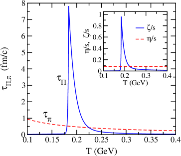
Figure 3.1: Temperature dependence of bulk and shear relaxation times. Inset shows $\zeta/s$ (see text) and $\eta/s=1/4\pi$.

Figure 3.2(a) shows time evolution of the shear pressure $\Phi$ and the magnitude of the bulk pressure $\Pi$. At early times $\tau\lesssim 2$ fm/c or equivalently at $T\gtrsim 1.2T_{c}$, shear dominates bulk. This implies that eccentricity-driven elliptic flow which develops early in the system would be controlled more by the shear pressure [Song:2009rh]. At later times (when $T\sim T_{c}$), the large value of $\zeta/s$ makes the bulk pressure dominant. This leads to sizeable entropy generation (Eq. (3.2)) and consequently enhanced particle production.

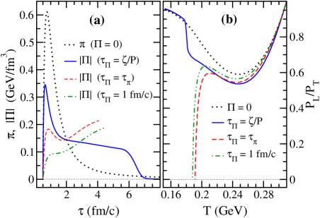
Figure 3.2: (a) Time evolution of shear stress in the absence of bulk ($\Pi=0$) and magnitude of bulk stress for $\tau_{\Pi}=\zeta/P$ and $\tau_{\Pi}=\tau_{\pi}$. The arrow indicates the time when $T_{c}$ is reached. (b) Temperature dependence of pressure anisotropy, $P_{L}/P_{T}$, for these three cases. The results are for initial $T=310$ MeV, $\tau_{0}=0.5$ fm/c and $\eta/s=1/4\pi$. The evolution is stopped when $P_{L}$ vanishes.

Figure 3.2(a) also compares the $\Pi$ evolution for bulk relaxation time, $\tau_{\Pi}$, calculated from Eq. (3.29) (solid line) and $\tau_{\Pi}=\tau_{\pi}$ (dashed line) and $\tau_{\Pi}=1$ fm/c (dashed-dotted line). At early times, the larger value of $\tau_{\Pi}$ in the latter cases (see Fig. 3.1) results in a relatively smaller growth of $|\Pi|$ as evident from Eq. (3.28). Near $T_{c}$, the rapid increase in $\zeta/s$ causes $|\Pi|$ to increase. Subsequently the longitudinal pressure $P_{L}=(P+\Pi-\Phi)$ vanishes leading to cavitation [Fries:2008ts, Rajagopal:2009yw, Torrieri:2008ip, Bhatt:2010cy]. In contrast, with our $\tau_{\Pi}$, this rise in $\zeta/s$ is overcompensated by a faster increase in $\tau_{\Pi}$ thereby slowing down the evolution of $\Pi$. This behaviour prevents the onset of cavitation and guarantees the applicability of hydrodynamics with bulk and shear up to temperatures well below $T_{c}$ into the hadronic phase. Furthermore, this slowing down of the medium followed by its rapid expansion, has the right trend to explain the identical-pion correlation measurements (Hanbury Brown-Twiss puzzle) [Paech:2006st, Pratt:2008qv].

The absence of cavitation in the present calculation is clearly evident in Fig. 3.2(b) which shows the variation of pressure anisotropy, $P_{L}/P_{T}=(P+\Pi-\Phi)/(P+\Pi+\Phi/2)$, with temperature. Near $T_{c}$, the longitudinal pressure $P_{L}$ vanishes if one assumes $\tau_{\Pi}=\tau_{\pi}$ (dashed line) or a constant value $\tau_{\Pi}=1$ fm/c (dashed-dotted line) leading to cavitation, whereas it is found to be positive for all temperatures with $\tau_{\Pi}$ derived here (solid line). In fact, we have found that in the latter case, cavitation is completely avoided for the entire range of $\zeta/s$ values ($0.5<\zeta/s<2.0$ near $T_{c}$) estimated in lattice QCD [Meyer:2007dy]. The sizeable difference between the $\Pi=0$ case (dot-dashed line) and the $\tau_{\Pi}=\zeta/P$ case (solid line) clearly underscores the importance of bulk pressure near $T_{c}$, which can have significant implications for the elliptic flow $v_{2}$ [Denicol:2009am] thus affecting the extraction of $\eta/s$. Further, the large bulk pressure when incorporated in the freezeout prescription could also affect the final particle abundances and spectra.

We have also found that the evolution of $\Pi$ is insensitive to the choice of initial conditions such as $\Pi(\tau_{0})=0$ and the Navier-Stokes value $-\zeta(T_{0})/\tau_{0}$. This is due to very small $\tau_{\Pi}$ at early times (or higher temperatures) which causes $\Pi$ to quickly lose the memory of its initial condition and to relax to the same value at $\tau\gtrsim 1$ fm/c.

3.4 Summary and conclusions

To summarize, we have presented a new derivation of the relativistic dissipative hydrodynamic equations from entropy considerations. We arrive at the same form of dissipative evolution equations as in the standard derivation but with all second-order transport coefficients such as the relaxation times and the entropy flux coefficients determined consistently within the same framework. We find that in the Bjorken scenario, although the bulk pressure can be large, the relaxation time derived here prevents the onset of cavitation due to the critical slowing down of bulk evolution near $T_{c}$.

In the next chapter, we employ the method developed here to derive relativistic viscous hydrodynamic equations for two different forms of the non-equilibrium single-particle distribution function. These equations are used to study thermal dilepton and hadron spectra within longitudinal scaling expansion of the matter formed in relativistic heavy-ion collisions. For consistency, the same non-equilibrium distribution function will be used in the particle production prescription as in the derivation of the viscous evolution equations.

Chapter 4 A consistent hydrodynamic approach to particle production

4.1 Introduction

Evolution of the strongly-interacting matter produced in high-energy heavy-ion collisions, when the system is close to local thermodynamic equilibrium, has been studied extensively within the framework of the relativistic dissipative hydrodynamics; for a recent review see Ref. [Heinz:2013th]. As the system expands and becomes dilute enough the hydrodynamic description breaks down, leading to a freezeout or a transition from the hydrodynamic description to a particle description [Cooper:1974mv]. The dissipative effects are important not only during the hydrodynamic evolution, but also in the particle production [Teaney:2003kp], and both have to be treated in a consistent manner. Moreover, the transport coefficients and relaxation times which constitute an external input to the hydrodynamic equations need to be in conformity with the theoretical framework used to derive the hydrodynamic equations [Jaiswal:2013fc]. Ad hoc choices or inconsistent treatments could significantly affect the final-state particle yields, spectra and other observables derived from them.

As already mentioned in the previous chapters, hydrodynamics is formulated as an order-by-order expansion in gradients of the hydrodynamic four-velocity $u^{\mu}$ where the ideal hydrodynamics is zeroth order and relativistic Navier-Stokes equation is first order in gradients; the latter violates causality. Derivation of the (causal) second-order dissipative hydrodynamic equations proceeds in a variety of ways [Romatschke:2009im]. For instance, in the derivations based on kinetic theory the non-equilibrium phase-space distribution function, $f(x,p)$, needs to be specified. This is commonly achieved by taking recourse to Grad’s 14-moment approximation [Grad]. The hydrodynamic equations are then derived by suitable coarse-graining of the microscopic dynamics. For consistency, the same $f(x,p)$ ought to be used in the particle-production prescription [Cooper:1974mv, McLerran:1984ay] as well. This important consideration has been overlooked in several hydrodynamic studies of heavy-ion collisions.

An alternate derivation of hydrodynamic equations starts from a generalized entropy four-current, $S^{\mu}$, expressed in terms of a few unknown coefficients and then invokes the second law of thermodynamics ($\partial_{\mu}S^{\mu}\geq 0$) [Romatschke:2009im]. These coefficients which are related to relaxation times for shear and bulk pressures remain undetermined, and have to be obtained from kinetic theory [Israel:1979wp, Muronga:2003ta]. Even then the bulk relaxation time remains ambiguous. Ideally, a single theoretical framework should give rise to dissipative evolution equations as well as determine these unknown coefficients [Jaiswal:2013fc]. The bulk relaxation time obtained in Ref. [Jaiswal:2013fc] exhibits critical slowing down near the QCD phase transition and does not lead to cavitation.

In this chapter, we employ the method of the previous chapter based on the entropy four-current to derive second-order viscous hydrodynamics corresponding to two different forms of the non-equilibrium distribution function. These distribution functions are formally different and one of them is used here for the first time to study the particle production in heavy-ion collisions. For consistency, we use the same non-equilibrium distribution function in the calculation of the particle spectra as in the derivation of the evolution equations. We perform a comparative numerical study of these two formalisms in the Bjorken scaling expansion. As an application, we study the production of thermal dileptons and hadrons in various scenarios.

4.2 Viscous hydrodynamics

From Eq. (2.75), the entropy four-current for particles obeying the Boltzmann statistics is given by [deGroot]

$$S^{\mu}(x)=-\int dp~{}p^{\mu}f\left(\ln f-1\right),$$ (4.1)

where $dp=gd{\bf p}/[(2\pi)^{3}\sqrt{{\bf p}^{2}+m^{2}}]$, $g$ and $m$ being the degeneracy factor and the particle rest mass, $p^{\mu}$ is the particle four-momentum, and $f\equiv f(x,p)$ is the single-particle phase-space distribution function. For a system close to equilibrium, $f$ can be written as $f=f_{0}+\delta f\equiv f_{0}(1+\phi)$, where the equilibrium distribution function is defined as $f_{0}=\exp(-\beta u\cdot p)$. Here $\beta\equiv 1/T$ is the inverse temperature, $u^{\mu}$ is defined in the Landau frame [deGroot], and we have assumed the baryo-chemical potential to be zero.

The divergence of $S^{\mu}$ reads

$$\partial_{\mu}S^{\mu} =-\int dp~{}p^{\mu}\left(\partial_{\mu}f\right)\ln f$$

$$=-\int dp~{}p^{\mu}\left[\phi(1+\phi/2)(\partial_{\mu}f_{0})+\phi(\partial_{\mu}\phi)f_{0}\right],$$ (4.2)

where in the second equality terms up to third order in gradients have been retained.

To proceed further, the non-equilibrium part of the distribution function $\delta f\equiv f_{0}\phi$ needs to be specified. In the present chapter, we consider two different forms of $\phi$. The first form is obtained using Grad’s 14-moment approximation [Grad] for the single-particle distribution function in orthogonal basis [Denicol:2012cn]. We propose

$$\phi_{1}=\frac{\Pi}{P}+\frac{p^{\mu}p^{\nu}\pi_{\mu\nu}}{2(\epsilon+P)T^{2}},$$ (4.3)

where corrections up to second order in momenta are present. Equation (4.3) has not been used before to study particle production in heavy-ion collisions. The second form is obtained by considering the corrections which are only quadratic in momenta [Dusling:2007gi]:

$$\phi_{2}=\frac{p^{\mu}p^{\nu}}{2(\epsilon+P)T^{2}}\left(\pi_{\mu\nu}+\frac{2}{5}\Pi\Delta_{\mu\nu}\right).$$ (4.4)

In Eqs. (4.3) and (4.4), $\epsilon$ and $P$ are the thermodynamic energy density and pressure, $\Pi$ the bulk viscous pressure, $\pi^{\mu\nu}$ the shear stress tensor, and $\Delta^{\mu\nu}=g^{\mu\nu}-u^{\mu}u^{\nu}$. The energy-momentum tensor can be expressed in terms of these quantities as $T^{\mu\nu}=\epsilon u^{\mu}u^{\nu}-(P+\Pi)\Delta^{\mu\nu}+\pi^{\mu\nu}$. Note that although the contributions due to shear in Eqs. (4.3) and (4.4) are identical, those due to bulk viscosity are distinct. In the following, we shall refer to analyses performed using Eqs. (4.3) and (4.4) as ‘Case 1’ and ‘Case 2’, respectively.

Performing the integrals in Eq. (4.2) as outlined in Ref. [Jaiswal:2013fc], we obtain

$$\partial_{\mu}S^{\mu}=-\beta\Pi\left[\theta+\!\beta_{0}\dot{\Pi}+\frac{4}{3}\beta_{0}\theta\Pi\right]+\beta\pi^{\mu\nu}\left[\sigma_{\mu\nu}-\beta_{2}\dot{\pi}_{\mu\nu}-\frac{4}{3}\beta_{2}\theta\pi_{\mu\nu}\right],$$ (4.5)

where $\beta_{0}$ and $\beta_{2}$ are functions of thermodynamic quantities $\epsilon$ and $T$, $\dot{X}\equiv u^{\mu}\partial_{\mu}X$, $\theta=\partial_{\mu}u^{\mu}$, and $\sigma^{\mu\nu}=\nabla^{\langle\mu\nu\rangle}$. The notation $A^{\langle\mu\nu\rangle}=\Delta^{\mu\nu}_{\alpha\beta}A^{\alpha\beta}$, where $\Delta^{\mu\nu}_{\alpha\beta}=[\Delta^{\mu}_{\alpha}\Delta^{\nu}_{\beta}+\Delta^{\mu}_{\beta}\Delta^{\nu}_{\alpha}-(2/3)\Delta^{\mu\nu}\Delta_{\alpha\beta}]/2$, represents the traceless symmetric projection orthogonal to $u^{\mu}$.

The second law of thermodynamics, $\partial_{\mu}S^{\mu}\geq 0$, is guaranteed to be satisfied if linear relationships between thermodynamical fluxes and extended thermodynamic forces are imposed. This leads to the following evolution equations for bulk and shear

$$\Pi =-\zeta\left[\theta+\beta_{0}\dot{\Pi}+\frac{4}{3}\beta_{0}\theta\Pi\right],$$ (4.6)

$$\pi^{\mu\nu} =2\eta\left[\sigma^{\mu\nu}-\beta_{2}\dot{\pi}^{\langle\mu\nu\rangle}-\frac{4}{3}\beta_{2}\theta\pi^{\mu\nu}\right],$$ (4.7)

where the coefficients of bulk and shear viscosity satisfy $\zeta,\eta\geq 0$. The bulk and shear relaxation times defined as $\tau_{\Pi}=\zeta\beta_{0}$ and $\tau_{\pi}=2\eta\beta_{2}$, can be obtained directly from the transport coefficients $\beta_{0}$ and $\beta_{2}$ which are determined explicitly in the above derivations.

For Case 1, the coefficients $\beta_{0}$ and $\beta_{2}$ become

$$\beta_{0}^{(1)}=1/P,\quad\beta_{2}^{(1)}=3/(\epsilon+P)+m^{2}\beta^{2}P/[2(\epsilon+P)^{2}],$$ (4.8)

whereas for Case 2, they reduce to

$$\beta_{0}^{(2)}=\frac{18}{5(\epsilon+P)}+\frac{3m^{2}\beta^{2}P}{5(\epsilon+P)^{2}},\quad\beta_{2}^{(2)}=\beta_{2}^{(1)}.$$ (4.9)

We note that although the relaxation time corresponding to shear ($\beta_{2}$) is the same for both the cases, that corresponding to bulk ($\beta_{0}$) is different. We stress that these coefficients have been obtained consistently within a single theoretical framework. This is in contrast to the standard derivation [Israel:1979wp], where the transport coefficients have to be estimated from an alternate theory.

4.3 Thermal dilepton and hadron production

Particle production is influenced by viscosity in two ways: first through the viscous hydrodynamic evolution of the system and second through corrections to the particle production rate via the non-equilibrium distribution function [Teaney:2003kp]. Hydrodynamic evolution was considered in the previous section; here we will concentrate on the thermal dilepton and hadron production rates in heavy-ion collisions. While the hadrons are emitted mostly in the final stages of the evolution, the dileptons are emitted at all stages and thus probe the entire temperature history of the system.

In the quark-gluon plasma (QGP) phase, the dominant production mechanism for dileptons is $q\bar{q}\rightarrow\gamma^{*}\rightarrow l^{+}l^{-}$, whereas in the hadronic phase the main contribution arises from $\pi^{+}\pi^{-}\rightarrow\rho^{0}\rightarrow l^{+}l^{-}$. The dilepton production rate for these processes is given by [rvogt]

$$\frac{dN}{d^{4}xd^{4}p}=g^{2}\int\frac{d^{3}\textbf{p}_{1}}{(2\pi)^{3}}\frac{d^{3}\textbf{p}_{2}}{(2\pi)^{3}}f(E_{1},T)f(E_{2},T)v_{rel}\sigma(M^{2})\delta^{4}(p-p_{1}-p_{2}),$$ (4.10)

where $p_{i}=(E_{i},\textbf{p}_{i})$ are the four momenta of the incoming particles having equal masses $m_{i}$ and relative velocity $v_{rel}=M(M^{2}-4m_{i}^{2})^{1/2}/2E_{1}E_{2}$. Further, $M$ and $\sigma(M^{2})$ are the dilepton invariant mass and production cross section, respectively. Substituting for $f=f_{0}+\delta f$ and retaining only the terms linear in $\delta f$, the dilepton production rate can be expressed as a sum of contributions due to ideal, shear and bulk:

$$\frac{dN}{d^{4}xd^{4}p}=\frac{dN^{(0)}}{d^{4}xd^{4}p}+\frac{dN^{(\pi)}}{d^{4}xd^{4}p}+\frac{dN^{(\Pi)}}{d^{4}xd^{4}p}.$$ (4.11)

For the case $M\gg T\gg m_{i}$, the equilibrium distribution functions can be approximated by the Maxwell-Boltzmann form $f(E,T)=\exp(-E/T)$ and $v_{rel}\simeq M^{2}/2E_{1}E_{2}$. In the QGP phase (for $q\bar{q}$ annihilation) we have $M^{2}g^{2}\sigma(M^{2})=(80\pi/9)\alpha^{2}$ (with $N_{f}$=2 and $N_{c}=3$) and in the hadronic phase (for $\pi^{+}\pi^{-}$ annihilation) we have $M^{2}g^{2}\sigma(M^{2})=(4\pi/3)\alpha^{2}|F_{\pi}(M^{2})|^{2}$ [rvogt]. The electromagnetic pion form factor is $|F_{\pi}(M^{2})|^{2}=m_{\rho}^{4}/[(m_{\rho}^{2}-M^{2})^{2}+m_{\rho}^{2}\Gamma_{\rho}^{2}]$, where $m_{\rho}=775$ MeV and $\Gamma_{\rho}=149$ MeV are the mass and decay width of the $\rho(770)$ meson [Song:2010fk].

With the above approximations, the integrals in Eq. (4.11) can be performed. The ideal part is given by [rvogt]

$$\frac{dN^{(0)}}{d^{4}xd^{4}p}=\frac{1}{2}~{}\frac{M^{2}g^{2}\sigma(M^{2})}{(2\pi)^{5}}~{}e^{-p_{0}/T}.$$ (4.12)

The shear viscosity contribution is the same for $\phi_{1}$ and $\phi_{2}$, Eqs. (4.3) and (4.4), and is given by [Dusling:2008xj]

$$\frac{dN^{(\pi)}}{d^{4}xd^{4}p}=\frac{2}{3}\left(\frac{p^{\mu}p^{\nu}}{2sT^{3}}\pi_{\mu\nu}\right)\frac{dN^{(0)}}{d^{4}xd^{4}p},$$ (4.13)

where $s=(\epsilon+P)/T$ is the equilibrium entropy density. The bulk viscosity contributions for $\phi_{1}$ is

$$\frac{dN^{(\Pi)}_{1}}{d^{4}xd^{4}p}=\frac{\Pi}{P}\,\frac{dN^{(0)}}{d^{4}xd^{4}p},$$ (4.14)

and that for $\phi_{2}$ can be expressed as [Bhatt:2011kx]

$$\frac{dN^{(\Pi)}_{2}}{d^{4}xd^{4}p}=\frac{2}{5sT^{3}}\left(\frac{M^{2}}{12}g^{\alpha\beta}-\frac{1}{3}p^{\alpha}p^{\beta}\right)\Delta_{\alpha\beta}\Pi\,\frac{dN^{(0)}}{d^{4}xd^{4}p}.$$ (4.15)

The hadron spectra are obtained using the Cooper-Frye freezeout prescription [Cooper:1974mv]

$$\frac{dN}{d^{2}p_{T}dy}=\frac{g}{(2\pi)^{3}}\int p_{\mu}d\Sigma^{\mu}f(x,p),$$ (4.16)

where, $d\Sigma^{\mu}$ represents the element of the three-dimensional freezeout hypersurface and $f(x,p)$ represents the phase-space distribution function at freezeout.

For the two cases discussed above we shall study the evolution of the hydrodynamic variables and their influence on the dilepton and hadron production rates.

4.4 Bjorken scenario

We consider the evolution of the system in longitudinal scaling expansion at vanishing net baryon number density [Bjorken:1982qr]. In terms of the Milne coordinates ($\tau,r,\varphi,\eta_{s}$), where $\tau=\sqrt{t^{2}-z^{2}}$ and $\eta_{s}=\tanh^{-1}(z/t)$, and with $u^{\mu}=(1,0,0,0)$, evolution equations for $\epsilon$, $\Phi\equiv-\tau^{2}\pi^{\eta_{s}\eta_{s}}$ and $\Pi$ become (see Appendix A for details)

$$\frac{d\epsilon}{d\tau} =-\frac{1}{\tau}\left(\epsilon+P+\Pi-\Phi\right),$$ (4.17)

$$\tau_{\pi}\frac{d\Phi}{d\tau} =\frac{4\eta}{3\tau}-\Phi-\frac{4\tau_{\pi}}{3\tau}\Phi,$$ (4.18)

$$\tau_{\Pi}\frac{d\Pi}{d\tau} =-\frac{\zeta}{\tau}-\Pi-\frac{4\tau_{\Pi}}{3\tau}\Pi.$$ (4.19)

The bulk and shear relaxation times $\tau_{\Pi}=\zeta\beta_{0}$ and $\tau_{\pi}=2\eta\beta_{2}$, reduce to

$$\tau_{\Pi}^{(1)}=\frac{\epsilon+P}{PT}\left(\frac{\zeta}{s}\right),\quad\tau_{\Pi}^{(2)}=\frac{18}{5T}\left(\frac{\zeta}{s}\right),\quad\tau_{\pi}=\frac{6}{T}\left(\frac{\eta}{s}\right),$$ (4.20)

for the two different forms of $\phi$, Eqs. (4.3) and (4.4).

Once the temperature evolution is known from the hydrodynamical model, the total dilepton spectrum is obtained by integrating the total rate over the space-time evolution of the system

$$\frac{dN_{1,2}}{d^{2}p_{T}dM^{2}dy}=A_{\perp}\int_{\tau_{0}}^{\tau_{fo}}d\tau~{}\tau\int_{-\infty}^{\infty}d\eta_{s}\left(\frac{1}{2}\frac{dN_{1,2}}{d^{4}xd^{4}p}\right),$$ (4.21)

where $A_{\perp}$ is the transverse area of the overlap zone of the colliding nuclei and, $\tau_{0}$ and $\tau_{fo}$ are the initial and freezeout times for the hydrodynamic evolution. We note that for the Bjorken expansion, $d^{4}x=A_{\perp}d\eta_{s}\tau d\tau$. For central ($b=0$) collisions, $A_{\perp}=\pi R_{A}^{2}$ where $R_{A}=1.2A^{1/3}$ is the nuclear radius, $A$ being the mass number of the colliding nuclei.

In $(\tau,r,\varphi,\eta_{s})$ coordinates, particle four momentum is $p^{\mu}=(m_{T}\cosh(y-\eta_{s}),~{}p_{T}\cos(\varphi_{p}-\varphi),~{}p_{T}\sin(\varphi_{p}-\varphi)/r,~{}m_{T}\sinh(y-\eta_{s})/\tau)$, where $m_{T}^{2}$ = $p_{T}^{2}+m^{2}$. The other factors appearing in the rate expressions, Eqs. (4.13)-(4.16), are then given by

$$p^{\alpha}p^{\beta}\pi_{\alpha\beta} = \frac{\Phi}{2}p_{T}^{2}-\Phi~{}m_{T}^{2}~{}\sinh^{2}(y-\eta_{s}),$$ (4.22)

$$p^{\alpha}p^{\beta}\Delta_{\alpha\beta} = -p_{T}^{2}-m_{T}^{2}~{}\sinh^{2}(y-\eta_{s}).$$ (4.23)

Similar to the dilepton spectra, the hadronic spectra can also be split up into three parts. Writing the momentum flux through the hypersurface element as $p_{\mu}d\Sigma^{\mu}=m_{T}\cosh(y-\eta_{s})\tau d\eta_{s}rdrd\varphi$, and performing the $\eta_{s}$ integration, we get for the ideal case,

$$\frac{dN^{(0)}}{d^{2}p_{T}dy}=\frac{g}{4\pi^{3}}m_{T}\tau_{fo}A_{\perp}K_{1}(z_{m}),$$ (4.24)

where $K_{n}$ are the modified Bessel functions of the second kind and $z_{m}\equiv m_{T}/T$. The contribution due to the shear viscosity to the hadron production reduces to

$$\frac{dN^{(\pi)}}{d^{2}p_{T}dy}=\frac{\Phi}{4(\epsilon+P)}\left[z_{p}^{2}-2z_{m}\frac{K_{2}(z_{m})}{K_{1}(z_{m})}\right]\frac{dN^{(0)}}{d^{2}p_{T}dy},$$ (4.25)

where $z_{p}\equiv p_{T}/T$. The bulk viscosity contribution in Case 1, Eq. (4.3), is calculated to be

$$\frac{dN^{(\Pi)}_{1}}{d^{2}p_{T}dy}=\frac{\Pi}{P}\frac{dN^{(0)}}{d^{2}p_{T}dy},$$ (4.26)

whereas in Case 2, Eq. (4.4), it reduces to

$$\frac{dN^{(\Pi)}_{2}}{d^{2}p_{T}dy}=\frac{-\Pi}{5(\epsilon+P)}\left[z_{p}^{2}+z_{m}\frac{K_{2}(z_{m})}{K_{1}(z_{m})}\right]\frac{dN^{(0)}}{d^{2}p_{T}dy}.$$ (4.27)

Here we have used the recurrence relation $K_{n+1}(z)=2nK_{n}(z)/z+K_{n-1}(z)$. It is important to note that the bulk viscosity contribution in Case 1 is negative, whereas that in Case 2 is positive ($\Pi<0$).

4.5 Numerical results and discussion

We now present numerical results for the Bjorken expansion of the medium for the initial temperature $T_{0}=310$ MeV and time $\tau_{0}=0.5$ fm/c, typical for the Relativistic Heavy-Ion Collider. The freezeout temperature was taken to be $T_{fo}=160$ MeV. Initial pressure configuration was assumed to be isotropic: $\Phi=0=\Pi$. We employ the equation of state of Refs. [Huovinen:2009yb, Bazavov:2009zn] based on a recent lattice QCD simulation. The shear viscosity to entropy density ratio $\eta/s$ was taken to be $1/4\pi$ corresponding to the conjectured lower bound obtained in Ref. [Kovtun:2004de]. For the bulk viscosity to entropy density ratio $\zeta/s$ at $T\geq T_{c}\approx 184$ MeV we adopted a parametrized form of the lattice QCD result; see Refs. [Meyer:2007dy, Rajagopal:2009yw]. For $T<T_{c}$, we parametrized $\zeta/s$ given in Ref. [Prakash:1993bt].

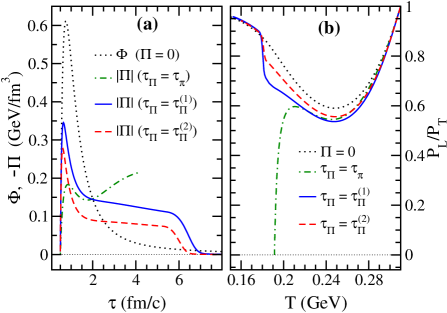
Figure 4.1: (a) Time evolution of shear, $\Phi$ and bulk, $\Pi$ viscous pressures, and (b) temperature dependence of the ratio of the longitudinal to transverse pressures $P_{L}/P_{T}$, for the various bulk relaxation times $\tau_{\Pi}$ defined in Eq. (4.20). Note that for $\tau_{\Pi}=\tau_{\pi}$, cavitation ($P_{L}<0$) sets in.

Figure 4.1(a) presents the time evolution of shear ($\Phi$) and bulk ($\Pi$) viscous pressures for the various bulk relaxation times $\tau_{\Pi}$ defined in Eq. (4.20). At times $\tau\gtrsim 3$ fm/c, corresponding to temperatures $T\lesssim 1.2~{}T_{c}$, the bulk dominates the shear pressure which can influence the particle production appreciably. The widely used choice $\tau_{\Pi}=\tau_{\pi}$ (dot-dashed line) leads to vanishing longitudinal pressure $P_{L}$ and cavitation [Rajagopal:2009yw] as is evident in Fig. 4.1(b). On the other hand, $\tau_{\Pi}=\tau_{\Pi}^{(1,2)}$ does not lead to cavitation as discussed in [Jaiswal:2013fc]. As $\tau_{\Pi}^{(1)}>\tau_{\Pi}^{(2)}$ at all times, the magnitude of $\Pi$ is found to be larger in Case 1 (solid line). This leads to enhanced pressure anisotropy, i.e., a larger departure of $P_{L}/P_{T}=(P+\Pi-\Phi)/(P+\Pi+\Phi/2)$ from unity.

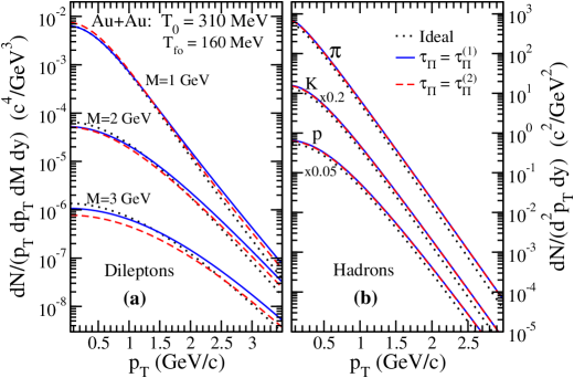
Figure 4.2: Particle spectra as a function of the transverse momentum $p_{T}$, for ideal and viscous hydrodynamics with bulk relaxation times $\tau_{\Pi}$ defined in Eq. (4.20) for (a) dileptons of invariant mass $M=1,~{}2,~{}3$ GeV/$c^{2}$, and (b) hadrons.

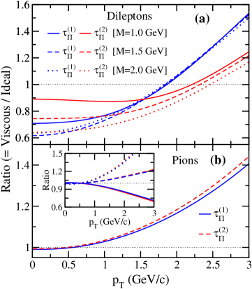
Figure 4.3: Ratios of particle yields for viscous and ideal hydrodynamics as a function of $p_{T}$, for the two bulk relaxation times $\tau_{\Pi}$ defined in Eq. (4.20) for (a) dileptons of invariant mass $M=1,~{}1.5,~{}2$ GeV/$c^{2}$, and (b) pions. Inset: Pion yields in various evolution and production scenarios scaled by the consistent second-order calculation for Case 1 (blue) and Case 2 (red). Solid lines: second-order evolution with ideal production rate; Dashed lines: second-order evolution with first-order correction to the production rate; Dotted lines: ideal evolution with first-order correction to the production rate.

Figure 4.2 displays dilepton and hadron transverse momentum spectra for the two choices of $\tau_{\Pi}$, in comparison with the ideal hydrodynamic calculation, and Fig. 4.3 shows the same spectra normalized by the ideal case. Note the enhancement of the dilepton spectra at high $p_{T}$, and suppression at low $p_{T}$ compared to the ideal case. The high-$p_{T}$ dileptons emerge predominantly at early times when the temperature and density are high. Viscosity slows down the cooling of the system [Muronga:2003ta] producing relatively larger number of hard dileptons. We observe that at high $p_{T}$, the viscous correction to the dilepton production rate due to shear is positive and dominates that due to bulk. The low-$p_{T}$ dileptons are produced mainly at later stages of the evolution when the negative correction due to the bulk viscosity dominates (Fig. 4.1) leading to the suppression of the spectra compared to the ideal case. Further for Case 2 (red lines), the $p_{T}^{2}$ dependence of the viscous correction, Eqs. (4.15) and (4.23), implies a smaller enhancement (suppression) at high (low) $p_{T}$, compared to Case 1 (blue lines). The $M$-dependent splitting is consistent with Eqs. (4.14)-(4.15).

Figure 4.3(b) shows the pion spectra scaled by the ideal case for the two choices of $\tau_{\Pi}$. The negative contribution from the bulk viscous correction for Case 1, Eq. (4.26), causes suppression of the ratio relative to Case 2, Eq. (4.27), where the correction is positive. More massive hadrons display qualitatively similar behaviour. Interestingly, at high $p_{T}$, dileptons and hadrons display opposite trends for $\tau_{\Pi}^{(1)}$ and $\tau_{\Pi}^{(2)}$ (Fig. 4.3).

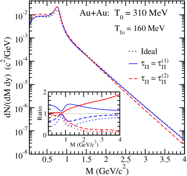
Figure 4.4: Dilepton yields as a function of the invariant mass $M$, in ideal and viscous hydrodynamics with the two bulk relaxation times $\tau_{\Pi}$ defined in Eq. (4.20). Inset: Same as Fig. 4.3 inset but for dileptons.

Finally, Fig. 4.4 shows the dilepton invariant mass spectra for the two cases (Eqs. (4.3)-(4.4)) in comparison with the ideal case. Results based on Case 1 (blue solid) are almost the same as those obtained in the ideal case at all invariant masses. This is essentially due to the fact that the invariant mass spectrum is dictated by the yields at small $p_{T}$ where the two are nearly identical (Fig. 4.2(a)). For Case 2 (red dashed) the spectrum exhibits enhanced low-mass and suppressed high-mass dilepton yields. This again can be traced back to the trend seen in Fig. 4.2(a). Note that the peak at $M=0.77$ GeV corresponds to the dilepton production from the $\rho(770)$ decay.

In contrast to the consistent approach adopted here, in Refs. [Monnai:2009ad, Dusling:2008xj], ideal hydrodynamical evolution was followed by particle production with non-ideal $f(x,p)$ up to first order in gradients. On the other hand, in Refs. [Bhatt:2011kx, Denicol:2009am, Dusling:2011fd], although the evolution was according to the second-order viscous hydrodynamics, the freezeout procedure involved ideal [Denicol:2009am] or Navier-Stokes [Bhatt:2011kx, Dusling:2011fd] corrections to the $f(x,p)$. To illustrate the differences arising due to inconsistent approaches, we show in the insets of Figs. 4.3 and 4.4, pion and dilepton production rates in various evolution and production scenarios scaled by the rate obtained in a consistent second-order calculation. We find that the results deviate from unity significantly which may have important implications for the on-going efforts to extract transport properties of QGP within hydrodynamic framework.

4.6 Summary and conclusions

We have derived viscous hydrodynamic equations for two different forms of the non-equilibrium distribution function, and have consistently used the same distribution function in the particle production prescription. In the Bjorken scaling expansion, we found appreciable differences between these two cases, for both dilepton and hadron production rates. Further, we showed that the dilepton and pion yields are significantly affected if the viscous effects in hydrodynamic evolution and particle production are not mutually consistent.

The derivation of second-order dissipative hydrodynamics from the entropy principles, as discussed in the present and previous chapter, is not complete in the sense that it misses several terms in the dynamical equations for dissipative quantities, compared to the derivations based on Boltzmann equation [Romatschke:2009im]. Moreover, as the non-equilibrium distribution function can be obtained by solving the Boltzmann equation, Grad’s 14-moment approximation is unnecessary in the formulation of dissipative hydrodynamics based on Boltzmann equation. In the next chapter, we derive second-order hydrodynamic evolution equations for the dissipative quantities, directly from their definitions, by solving the Boltzmann kinetic equation iteratively to obtain the non-equilibrium distribution function.

Chapter 5 Chapman-Enskog expansion and relativistic dissipative hydrodynamics

5.1 Introduction

The earliest theoretical formulation of relativistic dissipative hydrodynamics also known as first-order theories (order of gradients), are due to Eckart [Eckart:1940zz] and Landau-Lifshitz [Landau]. The Chapman-Enskog (CE) expansion has been the most common method to obtain first-order hydrodynamics from Boltzmann Equation (BE) [Chapman]. However, as discussed in Chapter 2, these theories involve parabolic differential equations and suffer from acausality and numerical instability. The derivation of second-order fluid-dynamics by Israel and Stewart (IS) from kinetic theory uses extended Grad’s method [Israel:1979wp]. The approach by Israel and Stewart may not guarantee stability but solves the acausality problem [Huovinen:2008te] at the cost of introducing two additional approximations: (a) 14-moment approximation for the distribution function and, (b) use of second moment of BE to obtain evolution equations for dissipative quantities.

Grad’s method, originally proposed for non-relativistic systems, was modified by Israel and Stewart so that it could be applicable to the relativistic case. In this extension, known as 14-moment approximation, the distribution function is Taylor expanded in powers of four-momenta around its local equilibrium value, see Chapter 3. Truncating the Taylor expansion at second-order in momenta results in 14 unknowns that have to be determined to describe the distribution function. This expansion implicitly assumes a converging series in powers of momenta. In addition, it is assumed that the order of expansion in 14-moment approximation (expanded as a series in momenta) coincides with that of gradient expansion of hydrodynamics. This is evident because Grad’s approximation truncated at second-order in momenta is not consistent with second-order hydrodynamics.

Another assumption inherent in IS derivation is the choice of second moment of the BE to extract the equation of motion for the dissipative quantities. This choice is arbitrary in the sense that once the distribution function is specified, any moment of the BE will lead to a closed set of equations for the dissipative currents but with different transport coefficients. In fact, it has been pointed out in Ref. [Denicol:2010xn] that instead of this ambiguous choice of the second-moment of BE by IS, the dissipative quantities can be obtained directly from their definition. Consistent and accurate formulation of relativistic dissipative hydrodynamics is still unresolved and is currently an active research area [Denicol:2010xn, Jaiswal:2013fc, Jaiswal:2012qm, El:2009vj, Denicol:2012cn].

In this chapter, we present an alternative derivation of hydrodynamic equations for dissipative quantities which do not make use of both these assumptions. We revisit the CE expansion of the distribution function using BE in Relaxation Time Approximation (RTA). The RTA for the collision term in BE is based on the assumption that the effect of the collisions is to exponentially restore the distribution function to its local equilibrium value. Although the information about the microscopic interactions of the constituent particles is not retained here, it is a reasonably good approximation to describe a system which is close to local equilibrium. Using this expansion, we derive the first and second-order equations of motion for the dissipative quantities from their definition. In one-dimensional boost-invariant Bjorken scenario, we demonstrate that our second-order results are in better agreement with transport results as compared to those obtained by using IS equations. We also illustrate that heuristic incorporation of higher-order corrections in viscous evolution equation significantly improves this agreement.

5.2 Chapman-Enskog expansion

Fluid dynamics is best described as a long-wavelength, low-frequency limit of an underlying microscopic theory. Further, BE governs the temporal evolution of single particle phase-space distribution function $f\equiv f(x,p)$ which provides a reliably accurate description of the microscopic dynamics in the dilute limit. With this motivation, our starting point for the derivation of hydrodynamic equations is relativistic BE with RTA for the collision term [Anderson_Witting]

$$p^{\mu}\partial_{\mu}f=-\frac{u\!\cdot\!p}{\tau_{R}}(f-f_{0})~{},$$ (5.1)

where, $p^{\mu}$ is the particle four-momentum, $u_{\mu}$ is the fluid four-velocity and $\tau_{R}$ is the relaxation time. We define the scalar product $u\cdot p\equiv u_{\mu}p^{\mu}$. The equilibrium distribution functions for Fermi, Bose, and Boltzmann particles ($r=1,-1,0$) are

$$f_{0}=\frac{1}{\exp(\beta\,u\!\cdot\!p-\alpha)+r}~{}.$$ (5.2)

Here, $\beta=1/T$ is the inverse temperature and $\alpha=\mu/T$ is the ratio of chemical potential to temperature.

In the CE expansion, the particle distribution function is expanded about its equilibrium value in powers of space-time gradients.

$$f=f_{0}+\delta f,\quad\delta f=\delta f^{(1)}+\delta f^{(2)}+\cdots,$$ (5.3)

where $\delta f^{(1)}$ is first-order in gradients, $\delta f^{(2)}$ is second-order and so on. The Boltzmann equation, (5.1), in the form $f=f_{0}-(\tau_{R}/u\cdot p)\,p^{\mu}\partial_{\mu}f$, can be solved iteratively as [Jaiswal:2013npa, Romatschke:2011qp]

$$f_{1}=f_{0}-\frac{\tau_{R}}{u\!\cdot\!p}\,p^{\mu}\partial_{\mu}f_{0},\quad f_{2}=f_{0}-\frac{\tau_{R}}{u\!\cdot\!p}\,p^{\mu}\partial_{\mu}f_{1},\quad\cdots$$ (5.4)

where $f_{1}=f_{0}+\delta f^{(1)}$ and $f_{2}=f_{0}+\delta f^{(1)}+\delta f^{(2)}$. To first and second-order in gradients, we obtain

$$\delta f^{(1)} =-\frac{\tau_{R}}{u\!\cdot\!p}\,p^{\mu}\partial_{\mu}f_{0},$$ (5.5)

$$\delta f^{(2)} =\frac{\tau_{R}}{u\!\cdot\!p}p^{\mu}p^{\nu}\partial_{\mu}\Big{(}\frac{\tau_{R}}{u\!\cdot\!p}\partial_{\nu}f_{0}\Big{)}.$$ (5.6)

For the sake of comparison, we also write down the Grad’s 14-moment expansion [Grad] in orders of momenta as suggested by IS [Israel:1979wp] in orthogonal basis [Denicol:2012cn],

$$\delta f=f_{0}\tilde{f}_{0}\left(\lambda_{\Pi}\Pi+\lambda_{n}n_{\alpha}p^{\alpha}+\lambda_{\pi}\pi_{\alpha\beta}p^{\alpha}p^{\beta}\right)+\mathcal{O}(p^{3}),$$ (5.7)

where, $\tilde{f}_{0}=1-rf_{0}$ and $\lambda_{\Pi}$, $\lambda_{n}$, $\lambda_{\pi}$ are determined from the definition of the dissipative quantities, Eqs. (5.10)-(5.12). Since hydrodynamics involves expansion in orders of gradients, hence for consistency, CE should be preferred over 14-moment approximation in derivation of hydrodynamic equations.

5.3 Relativistic hydrodynamics

The conserved energy-momentum tensor and particle current can be expressed in terms of distribution function, as described in Chapter 2,

$$T^{\mu\nu} =\int dp\ p^{\mu}p^{\nu}f=\epsilon u^{\mu}u^{\nu}-(P+\Pi)\Delta^{\mu\nu}+\pi^{\mu\nu},$$

$$N^{\mu} =\int dp\ p^{\mu}f=nu^{\mu}+n^{\mu},$$ (5.8)

where $dp=gd{\bf p}/[(2\pi)^{3}\sqrt{{\bf p}^{2}+m^{2}}]$, $g$ and $m$ being the degeneracy factor and particle mass. In the tensor decompositions, $\epsilon,P,n$ are respectively energy density, pressure, net number density, and $\Delta^{\mu\nu}=g^{\mu\nu}-u^{\mu}u^{\nu}$ is the projection operator on the three-space orthogonal to the hydrodynamic four-velocity $u^{\mu}$ defined in the Landau frame: $T^{\mu\nu}u_{\nu}=\epsilon u^{\mu}$. The metric tensor is $g^{\mu\nu}\equiv\mathrm{diag}(+,-,-,-)$. The bulk viscous pressure $(\Pi)$, shear stress tensor $(\pi^{\mu\nu})$ and particle diffusion current $(n^{\mu})$ are the dissipative quantities.

Energy-momentum conservation, $\partial_{\mu}T^{\mu\nu}=0$ and current conservation, $\partial_{\mu}N^{\mu}=0$, yields the fundamental evolution equations for $n$, $\epsilon$ and $u^{\mu}$

$$\dot{\epsilon}+(\epsilon+P+\Pi)\theta-\pi^{\mu\nu}\nabla_{(\mu}u_{\nu)} =0,$$

$$(\epsilon+P+\Pi)\dot{u}^{\alpha}-\nabla^{\alpha}(P+\Pi)+\Delta^{\alpha}_{\nu}\partial_{\mu}\pi^{\mu\nu} =0,$$

$$\dot{n}+n\theta+\partial_{\mu}n^{\mu} =0~{}.$$ (5.9)

We use the standard notation $\dot{A}=u^{\mu}\partial_{\mu}A$ for co-moving derivative, $\nabla^{\alpha}=\Delta^{\mu\alpha}\partial_{\mu}$ for space-like derivative, $\theta=\partial_{\mu}u^{\mu}$ for expansion scalar and $A^{(\alpha}B^{\beta)}=(A^{\alpha}B^{\beta}+A^{\beta}B^{\alpha})/2$ for symmetrization.

Even if the equation of state relating $\epsilon$ and $P$ is provided, the system of Eqs. (5.3) is not closed unless the dissipative quantities $\Pi$, $n^{\mu}$ and $\pi^{\mu\nu}$ are specified. To obtain the expressions for these dissipative quantities, we write them using Eq. (5.3) in terms of away from equilibrium part of the distribution functions, $\delta f$, as

$$\Pi =-\frac{\Delta_{\alpha\beta}}{3}\int dp\,p^{\alpha}p^{\beta}\delta f,$$ (5.10)

$$n^{\mu} =\Delta^{\mu}_{\alpha}\int dp\,p^{\alpha}\delta f,$$ (5.11)

$$\pi^{\mu\nu} =\Delta^{\mu\nu}_{\alpha\beta}\int dp\,p^{\alpha}p^{\beta}\delta f,$$ (5.12)

where $\Delta^{\mu\nu}_{\alpha\beta}=[\Delta^{\mu}_{\alpha}\Delta^{\nu}_{\beta}+\Delta^{\mu}_{\beta}\Delta^{\nu}_{\alpha}-(2/3)\Delta^{\mu\nu}\Delta_{\alpha\beta}]/2$.

The first-order dissipative equations can be obtained from Eqs. (5.10)-(5.12) using $\delta f=\delta f^{(1)}$ from Eq. (5.5)

$$\Pi =-\frac{\Delta_{\alpha\beta}}{3}\!\!\int\!\!dp\,p^{\alpha}p^{\beta}\left(-\frac{\tau_{R}}{u\!\cdot\!p}\,p^{\gamma}\partial_{\gamma}f_{0}\right),$$ (5.13)

$$n^{\mu} =\Delta^{\mu}_{\alpha}\!\!\int\!\!dp\,p^{\alpha}\left(-\frac{\tau_{R}}{u\!\cdot\!p}\,p^{\gamma}\partial_{\gamma}f_{0}\right),$$ (5.14)

$$\pi^{\mu\nu} =\Delta^{\mu\nu}_{\alpha\beta}\int dp\ p^{\alpha}p^{\beta}\left(-\frac{\tau_{R}}{u\!\cdot\!p}\,p^{\gamma}\partial_{\gamma}f_{0}\right).$$ (5.15)

Assuming the relaxation time $\tau_{R}$ to be independent of four-momenta, the integrals in Eqs. (5.13)-(5.15) reduce to

$$\Pi=-\tau_{R}\beta_{\Pi}\theta,~{}~{}n^{\mu}=\tau_{R}\beta_{n}\nabla^{\mu}\alpha,~{}~{}\pi^{\mu\nu}=2\tau_{R}\beta_{\pi}\sigma^{\mu\nu},$$ (5.16)

where $\sigma^{\mu\nu}=\Delta^{\mu\nu}_{\alpha\beta}\nabla^{\alpha}u^{\beta}$. The coefficients $\beta_{\Pi},~{}\beta_{n}$ and $\beta_{\pi}$ are found to be

$$\beta_{\Pi}= ~{}\frac{1}{3}\left(1-3c_{s}^{2}\right)(\epsilon+P)-\frac{2}{9}(\epsilon-3P)-\frac{m^{4}}{9}\left<(u\!\cdot\!p)^{-2}\right>_{0},$$ (5.17)

$$\beta_{n}= ~{}-\frac{n^{2}}{\beta(\epsilon+P)}+\frac{2\left<1\right>_{0^{-}}}{3\beta}+\frac{m^{2}}{3\beta}\left<(u\!\cdot\!p)^{-2}\right>_{0},$$ (5.18)

$$\beta_{\pi}= ~{}\frac{4P}{5}+\frac{\epsilon-3P}{15}-\frac{m^{4}}{15}\left<(u\!\cdot\!p)^{-2}\right>_{0},$$ (5.19)

where $\left<\cdots\right>_{0}=\int dp(\cdots)f_{0}$, and $c_{s}^{2}=(dP/d\epsilon)_{s/n}$ is the adiabatic speed of sound squared ($s$ being the entropy density). It is interesting to note that these coefficients are in perfect agreement with those obtained in the Ref. [Denicol:2010xn] in which the evolution equations are derived directly from their definition. This is due to the fact that in Ref. [Denicol:2010xn], the coefficients $\beta_{\Pi},~{}\beta_{n}$ and $\beta_{\pi}$, are associated with first-order terms and do not involve 14-moment approximation. In the massless limit, $\beta_{\pi}=4P/5$ is also in agreement with that obtained in Ref. [Romatschke:2011qp] employing CE expansion in BE with medium-dependent masses.

In the process to obtain second-order equations, we discover that CE expansion for the distribution function does not support derivation of hydrodynamic evolution equations from arbitrary moment choice of BE. Using the definition of dissipative quantities to obtain their evolution equations comes naturally when employing CE expansion as demonstrated while deriving first-order equations, Eq. (5.16). Second-order evolution equations can also be obtained similarly by substituting $\delta f=\delta f^{(1)}+\delta f^{(2)}$ from Eqs. (5.5) and (5.6) in Eqs. (5.10)-(5.12).

$$\frac{\Pi}{\tau_{R}}= \ \frac{\Delta_{\alpha\beta}}{3}\int dp\,p^{\alpha}p^{\beta}\left[\frac{p^{\gamma}}{u\!\cdot\!p}\partial_{\gamma}f_{0}-\frac{p^{\gamma}p^{\rho}}{u\!\cdot\!p}\partial_{\gamma}\Big{(}\frac{\tau_{R}}{u\!\cdot\!p}\partial_{\rho}f_{0}\Big{)}\right],$$ (5.20)

$$\frac{n^{\mu}}{\tau_{R}}= -\Delta^{\mu}_{\alpha}\int dp\,p^{\alpha}\left[\frac{p^{\gamma}}{u\!\cdot\!p}\partial_{\gamma}f_{0}-\frac{p^{\gamma}p^{\rho}}{u\!\cdot\!p}\partial_{\gamma}\Big{(}\frac{\tau_{R}}{u\!\cdot\!p}\partial_{\rho}f_{0}\Big{)}\right],$$ (5.21)

$$\frac{\pi^{\mu\nu}}{\tau_{R}}= -\Delta^{\mu\nu}_{\alpha\beta}\int dp\,p^{\alpha}p^{\beta}\left[\frac{p^{\gamma}}{u\!\cdot\!p}\partial_{\gamma}f_{0}-\frac{p^{\gamma}p^{\rho}}{u\!\cdot\!p}\partial_{\gamma}\Big{(}\frac{\tau_{R}}{u\!\cdot\!p}\partial_{\rho}f_{0}\Big{)}\right].$$ (5.22)

The derivatives of equilibrium distribution function ($\partial_{\mu}f_{0},~{}\partial_{\mu}\partial_{\nu}f_{0}$) appearing in above equations can be obtained by successively differentiating Eq. (5.2). The momentum integrations can be decomposed into hydrodynamic tensor degrees of freedom via the definitions:

$$I^{\mu_{1}\cdots\mu_{n}}_{(m)}\equiv\int\frac{dp}{(u\!\cdot\!p)^{m}}p^{\mu_{1}}\cdots p^{\mu_{n}}f_{0}=I_{n0}^{(m)}u^{\mu_{1}}\cdots u^{\mu_{n}}+I_{n1}^{(m)}(\Delta^{\mu_{1}\mu_{2}}u^{\mu_{3}}\cdots u^{\mu_{n}}+\mathrm{perms})+\cdots,$$ (5.23)

where ‘perms’ denotes all non-trivial permutations of the Lorentz indices. We similarly define $J^{\mu_{1}\mu_{2}\cdots\mu_{n}}_{(m)}$ where the momentum integrals are weighted with $f_{0}\tilde{f}_{0}$, and are tensor decomposed with coefficients $J_{nq}^{(m)}$.

After performing the integration, the relaxation time appearing on the right hand side of Eqs. (5.20)-(5.22) are absorbed using the first-order equations for the dissipative quantities, Eq. (5.16). Using the identity $\nabla^{\mu}\beta=-\beta\dot{u}^{\mu}+[n/(\epsilon+P)]\nabla^{\mu}\alpha+\mathcal{O}(\delta^{2})$, the terms containing derivatives of the relaxation time cancel each other up to second-order in gradients and hence the right hand side of Eqs. (5.20)-(5.22) can be made independent of $\tau_{R}$, see Appendix B. The second-order evolution equations of the dissipative quantities are finally obtained as

$$\frac{\Pi}{\tau_{R}}= -\dot{\Pi}-\beta_{\Pi}\theta-\delta_{\Pi\Pi}\Pi\theta+\lambda_{\Pi\pi}\pi^{\mu\nu}\sigma_{\mu\nu}-\tau_{\Pi n}n\cdot\dot{u}-\lambda_{\Pi n}n\cdot\nabla\alpha-\ell_{\Pi n}\partial\cdot n~{},$$ (5.24)

$$\frac{n^{\mu}}{\tau_{R}}= -\dot{n}^{\langle\mu\rangle}+\beta_{n}\nabla^{\mu}\alpha-n_{\nu}\omega^{\nu\mu}-\lambda_{nn}n^{\nu}\sigma_{\nu}^{\mu}-\delta_{nn}n^{\mu}\theta+\lambda_{n\Pi}\Pi\nabla^{\mu}\alpha-\lambda_{n\pi}\pi^{\mu\nu}\nabla_{\nu}\alpha$$

$$-\tau_{n\pi}\pi_{\nu}^{\mu}\dot{u}^{\nu}+\tau_{n\Pi}\Pi\dot{u}^{\mu}+\ell_{n\pi}\Delta^{\mu\nu}\partial_{\gamma}\pi_{\nu}^{\gamma}-\ell_{n\Pi}\nabla^{\mu}\Pi~{},$$ (5.25)

$$\frac{\pi^{\mu\nu}}{\tau_{R}}= -\dot{\pi}^{\langle\mu\nu\rangle}+2\beta_{\pi}\sigma^{\mu\nu}+2\pi_{\gamma}^{\langle\mu}\omega^{\nu\rangle\gamma}-\tau_{\pi\pi}\pi_{\gamma}^{\langle\mu}\sigma^{\nu\rangle\gamma}-\delta_{\pi\pi}\pi^{\mu\nu}\theta+\lambda_{\pi\Pi}\Pi\sigma^{\mu\nu}-\tau_{\pi n}n^{\langle\mu}\dot{u}^{\nu\rangle}$$

$$+\lambda_{\pi n}n^{\langle\mu}\nabla^{\nu\rangle}\alpha+\ell_{\pi n}\nabla^{\langle\mu}n^{\nu\rangle}~{},$$ (5.26)

where $\omega^{\mu\nu}=(\nabla^{\mu}u^{\nu}-\nabla^{\nu}u^{\mu})/2$ is the definition of the vorticity tensor. All the coefficients in the above equations have been obtained in terms of $\beta$ and the integral coefficients $I_{nq}^{(m)}$ and $J_{nq}^{(m)}$, see Appendix B. It is clear that in Eqs. (5.24)-(5.26), the Boltzmann relaxation time $\tau_{R}$ can be replaced by those of the individual dissipative quantities $\tau_{\Pi},~{}\tau_{n},~{}\tau_{\pi}$. At this stage, it seems as though the three relaxation times $\tau_{\Pi},~{}\tau_{n},~{}\tau_{\pi}$ are all equal to $\tau_{R}$. This is because the collision term in the BE, Eq. (5.1) is written in RTA which does not entirely capture the microscopic interactions. This apparent equality vanishes if the first-order equation, Eq. (5.16) is compared with the relativistic Navier-Stokes equations for dissipative quantities ($\Pi=-\zeta\theta$, $n^{\mu}=\kappa\nabla^{\mu}\alpha$ and $\pi^{\mu\nu}=2\eta\sigma^{\mu\nu}$). The dissipative relaxation times are then obtained in terms of first-order transport coefficients $\zeta,~{}\kappa$ and $\eta$ which can be calculated independently taking into account the full microscopic behaviour of the system [Kovtun:2004de, Meyer:2007dy].

We remark that although the form of the evolution equations for dissipative quantities obtained here, Eqs. (5.24)-(5.26), are the same as those obtained in the previous calculations using both 14-moment approximation and second moment of BE [Betz:2008me], the coefficients obtained are different. In the following discussion, we refer to the results in Ref. [Betz:2008me] as the IS results although the power counting scheme differs from the one employed originally by Israel and Stewart.

For the special case of a system consisting of single species of massless Boltzmann gas, we find that

$$\beta_{\pi}=\frac{4P}{5},\quad\tau_{\pi\pi}=\frac{10}{7},\quad\delta_{\pi\pi}=\frac{4}{3};$$ (5.27)

while these coefficients obtained via IS approach are [Betz:2008me]

$$\beta_{\pi}^{\rm{IS}}=\frac{2P}{3},\quad\tau_{\pi\pi}^{\rm{IS}}=2,\quad\delta_{\pi\pi}^{\rm{IS}}=\frac{4}{3}.$$ (5.28)

In this limit, although the coefficients of $\pi^{\mu\nu}\theta$ are same for both the cases ($\delta_{\pi\pi}=\delta_{\pi\pi}^{\rm{IS}}$), the coefficient of $\sigma^{\mu\nu}$ and $\pi_{\gamma}^{\langle\mu}\sigma^{\nu\rangle\gamma}$ are different ($\beta_{\pi}\neq\beta_{\pi}^{\rm{IS}},~{}\tau_{\pi\pi}\neq\tau_{\pi\pi}^{\rm{IS}}$).

We note that CE expansion, as opposed to 14-moment approximation, can be done iteratively to arbitrarily higher orders. Hence using CE expansion, dissipative hydrodynamic equations of any order can in principle be derived. To obtain $n$th-order evolution equations for dissipative quantities, $\delta f=\delta f^{(1)}+\delta f^{(2)}+\cdots+\delta f^{(n)}$ should be used in Eqs. (5.10)- (5.12). For instance, substitution of $\delta f=\delta f^{(1)}+\delta f^{(2)}+\delta f^{(3)}$ in Eqs. (5.10)-(5.12) will eventually lead to third-order evolution equations. Derivation of third-order hydrodynamics, as outlined above, is done in Chapter 7.

5.4 Numerical results and discussions

To demonstrate the numerical significance of the new coefficients derived here, we consider evolution in the boost invariant Bjorken case of a massless Boltzmann gas ($\epsilon=3P$) at vanishing net baryon number density [Bjorken:1982qr]. In terms of the Milne co-ordinates $(\tau,x,y,\eta_{s})$, where $\tau=\sqrt{t^{2}-z^{2}}$ and $\eta_{s}=\tanh^{-1}(z/t)$, the initial four-velocity becomes $u^{\mu}=(1,0,0,0)$. For this scenario, $\Pi=n^{\mu}=0$, and the evolution equations for $\epsilon$, $\Phi\equiv-\tau^{2}\pi^{\eta_{s}\eta_{s}}$ reduces to (see Appendix A for details)

$$\frac{d\epsilon}{d\tau} =-\frac{1}{\tau}\left(\epsilon+P-\Phi\right),$$ (5.29)

$$\frac{d\Phi}{d\tau} =-\frac{\Phi}{\tau_{R}}+\beta_{\pi}\frac{4}{3\tau}-\lambda\frac{\phi}{\tau}.$$ (5.30)

The second-order transport coefficients simplify to

$$\lambda\equiv\frac{1}{3}\tau_{\pi\pi}+\delta_{\pi\pi}=\frac{38}{21},\quad\lambda^{\rm{IS}}=2.$$ (5.31)

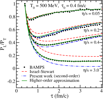
Figure 5.1: Time evolution of $P_{L}/P_{T}$ in BAMPS (dots), IS (dashed lines), present work (dashed-dotted line), and a heuristic higher-order approximation (solid line) for isotropic initial pressure configuration $(\Phi_{0}=0)$.

Initial temperature $T_{0}=500$ MeV at proper time $\tau_{0}=0.4$ fm/c are chosen to solve the coupled differential Eqs. (5.29) and (5.30). These values correspond to LHC initial conditions [El:2007vg]. We assume isotropic initial pressure configuration i.e. $\Phi_{0}=0$. Fig. 5.1, shows the proper time dependence of pressure anisotropy defined as $P_{L}/P_{T}=(P-\Phi)/(P+\Phi/2)$. The dashed and dashed-dotted lines represent the results from IS theory and our second-order results, respectively. The dots correspond to the results of a transport model, the Boltzmann Approach of MultiParton Scatterings (BAMPS), which is based on parton cascade simulations [El:2009vj, Xu:2004mz]. The calculations in BAMPS are performed with variable values for the cross section such that the shear viscosity to entropy density ratio is a constant.

We note that the results from IS theory always overestimate the pressure anisotropy as compared to the transport results even for viscosities as small as $\eta/s=0.05$. It is evident from the figure that our results are in better agreement with BAMPS as compared to the results of IS. For very high viscosity, i.e., for $\eta/s=3.0$, although at early times we have a better agreement with BAMPS as compared to IS, at later times there is a large deviation. This disagreement may be attributed to the fact that the present hydrodynamic calculation is terminated at second-order in gradients. Inclusion of higher-order corrections may improve the agreement of dissipative hydrodynamic calculation results with those obtained using BAMPS as illustrated in the following.

In Ref. [El:2009vj], while performing a third-order calculation it was demonstrated that within one-dimensional scaling expansion, the higher-order gradient terms can acquire the form $(\frac{\Phi}{\epsilon})^{n}\frac{\epsilon}{\tau}$, where, $n=r-1$ for $r$th-order corrections. The other forms of higher-order corrections is reducible to this structure through lower-order evolution equations. Here we assume a similar heuristic expression for higher-order corrections

$$\frac{d\Phi}{d\tau}=-\frac{\Phi}{\tau_{R}}+\beta_{\pi}\frac{4}{3\tau}-\lambda\frac{\Phi}{\tau}-\chi\frac{\Phi^{2}}{\beta_{\pi}\tau},$$ (5.32)

where the coefficient $\chi$ contains corrections to shear stress evolution due to higher-order gradients. This coefficient can be obtained by demanding that the above equation be valid for a free streaming of particles in the limit of infinite shear viscosity ($\eta\to\infty$). In this limit, $\tau_{R}\to\infty$, and within one-dimensional scaling expansion the energy density evolves as $\dot{\epsilon}=-\epsilon/\tau$ which implies that $\dot{P}=-P/\tau$. For this case, using Eq. (5.29), we arrive at $\Phi=\epsilon/3=P$ which indicates disappearance of the longitudinal pressure. Substituting all these in Eq. (5.32), we obtain $\chi=36/175$.

Fig. 5.1, also shows $P_{L}/P_{T}$ evolution for the results obtained after including higher-order corrections (solid lines). We observe that the incorporation of higher-order corrections significantly improves the agreement with BAMPS. It is important to note that the BAMPS calculations are performed with the form of the collision term that captures the realistic microscopic interactions whereas the derivation of dissipative hydrodynamic equations in this chapter uses RTA for the collision term. Within CE formalism, more sophisticated ways exist for solving the BE, for eg., by using variational methods [Chapman] or by considering momentum dependent relaxation time [Prakash:1993bt, Teaney:2009qa]. It is, in principle, possible to derive second-order dissipative hydrodynamic evolution equations using momentum dependent relaxation time provided the dependence is specified explicitly. While this is left for future work, we observe that the near perfect agreement of the BAMPS results with those obtained using higher-order corrections clearly suggest that the momentum independent relaxation time for the BE used in the present derivation is sufficiently reliable for the range of $\eta/s$ considered here. However, the results obtained by using a momentum dependent relaxation time may show a better agreement with BAMPS data already at second-order.

RTA for the collision term assumes that the effect of the collisions is to restore the distribution function to its local equilibrium value exponentially. This is a very good approximation as long as the deviations from local equilibrium are small. As discussed above, we find that for the range of $\eta/s$ considered here, the deviation from equilibrium is not so large because the RTA is still valid. It is also important to note that large values of $\eta/s$ ($>0.4$) are not relevant to the physics of strongly coupled systems like Quark Gluon Plasma (QGP). The QGP formed at RHIC and LHC behaves as a near perfect fluid with a small estimated $\eta/s\approx 0.08-0.2$ [Romatschke:2007mq, Song:2010mg]. Using second-order evolution equations derived here, we get reasonably good agreement with BAMPS results for $\eta/s\leq 0.4$ (Fig. 5.1). This suggests that BE with RTA for the collision term can be successfully applied in understanding the hydrodynamic behaviour of QGP formed in relativistic heavy-ion collisions.

5.5 Summary and conclusions

To summarize, we have presented a new derivation of relativistic second-order hydrodynamics from BE. We use Chapman-Enskog expansion for out of equilibrium distribution function instead of 14-moment approximation and derive evolution equations for dissipative quantities directly from their definitions rather than employing second moment of Boltzmann equation. In this new approach, we get rid of two powerful assumptions of Israel-Stewart kind of derivation which is 14-moment approximation and choice of second moment of Boltzmann equation. Although the form of the evolution equation remains the same, the coefficients are found to be different. For small $\eta/s$, our second-order results show reasonably good agreement with the parton cascade BAMPS for the $P_{L}/P_{T}$ evolution. We find that heuristic inclusion of higher-order corrections in shear evolution equation significantly improves the agreement with transport calculation for large $\eta/s$ as well. This concurrence also suggests that relaxation time approximation for the collision term in Boltzmann equation is reasonably accurate when applied to heavy-ion collisions.

A very important consequence of Chapman-Enskog like expansion is that, unlike Grad’s approximation which is linear in dissipative quantities, higher-order nonlinear corrections to the equilibrium distribution function can also be obtained. This has interesting implications for the formulation of dissipative hydrodynamics as well as its implementation to the physics of high-energy heavy-ion collisions. For example, a different form of nonequilibrium distribution function in the particle production prescription [Cooper:1974mv], may affect the observables significantly. In the next chapter, we derive an explicit expression for the viscous correction to the equilibrium distribution function up to second-order in gradients by employing Chapman-Enskog like expansion. We compare the hadronic spectra and longitudinal Hanbury Brown-Twiss (HBT) radii obtained using this alternate form of the viscous correction and Grad’s 14-moment approximation.

Chapter 6 Chapman-Enskog vs Grad’s methods: Effects on spectra and HBT radii

6.1 Introduction

The Standard Model of relativistic heavy-ion collisions relies on relativistic hydrodynamics to simulate the intermediate-stage evolution of the high-energy-density fireball formed in these collisions [Heinz:2013th]. Recent simulations generally make use of some version of the Müller-Israel-Stewart second-order theory of causal dissipative hydrodynamics [Israel:1979wp, Muronga:2003ta]. Hydrodynamics has achieved remarkable success in explaining, for example, the observed mass ordering of the elliptic flow [Adams:2005dq, Adcox:2004mh, Song:2013qma], higher harmonics of the azimuthal anisotropic flow [Adare:2011tg, Chatrchyan:2013kba], and the ridge and shoulder structure in long-range rapidity correlations [ATLAS:2012at]. The recently measured correlators between event planes of different harmonics [Jia:2012sa] too can be understood qualitatively within event-by-event hydrodynamics [Qiu:2012uy]. Notwithstanding these successes, the basic formulation of the dissipative hydrodynamic equations continues to be an area of considerable activity, largely because of the ambiguities arising due to the variety of ways in which these equations can be derived [El:2009vj, Romatschke:2009im, Denicol:2012cn, Jaiswal:2012qm, Jaiswal:2013fc, Jaiswal:2013npa, Bazow:2013ifa].

For a system that is out of equilibrium, the existence of thermodynamic gradients results in thermodynamic forces, which give rise to various transport phenomena. To quantify these nonequilibrium effects, it is convenient to first specify the nonequilibrium phase-space distribution function $f(x,p)$ and then calculate the various transport coefficients. In the context of hydrodynamics, two most commonly used methods to determine the form of the distribution function close to local thermodynamic equilibrium are: (1) Grad’s 14-moment approximation [Grad] and (2) the Chapman-Enskog method [Chapman]. Although both the methods involve expanding $f(x,p)$ around the equilibrium distribution function $f_{0}(x,p)$, there are important differences.

In the relativistic version of Grad’s 14-moment approximation, the small deviation from equilibrium is usually approximated by means of a Taylor-like series expansion in momenta truncated at quadratic order [Israel:1979wp, Romatschke:2009im]. Further, the 14 coefficients in this expansion are assumed to be linear in dissipative fluxes. However, it is not apparent why a power series in momenta should be convergent and whether one is justified in making such an ansatz, without a small expansion parameter.

The Chapman-Enskog method, on the other hand, aims at obtaining a perturbative solution of the Boltzmann transport equation using the Knudsen number (ratio of mean free path to a typical macroscopic length) as a small expansion parameter. This is equivalent to making a gradient expansion about the local equilibrium distribution function [deGroot]. This method of obtaining the form of the nonequilibrium distribution function is consistent [Jaiswal:2013npa] with dissipative hydrodynamics which is also formulated as a gradient expansion.

The above two methods have been compared and shortcomings of Grad’s approximation have been pointed out in the literature [velasco, Calzetta:2013vma, Tsumura:2013uma]. In spite of these shortcomings, the derivations of relativistic second-order dissipative hydrodynamic equations, as well as particle-production prescriptions, rely almost exclusively on Grad’s approximation. The Chapman-Enskog method, on the other hand, has seldom been employed in the hydrodynamic modelling of the relativistic heavy-ion collisions. The focus of this chapter is to explore the applicability of the latter method.

In this chapter, the Boltzmann equation in the relaxation-time approximation is solved iteratively, which results in a Chapman-Enskog-like expansion of the nonequilibrium distribution function. Truncating the expansion at the second order, we derive an explicit expression for the viscous correction to the equilibrium distribution function. We compare the hadronic spectra and longitudinal Hanbury Brown-Twiss (HBT) radii obtained using the form of the viscous correction derived here and Grad’s 14-moment approximation, within one dimensional scaling expansion. We find that at large transverse momenta, the present method yields smaller hadron multiplicities. We also show analytically that while Grad’s approximation leads to the violation of the experimentally observed $1/\sqrt{m_{T}}$ scaling of HBT radii [Bearden:2001sy, Adcox:2002uc], the viscous correction obtained here does not exhibit such unphysical behaviour. Finally, we demonstrate the rapid convergence of the Chapman-Enskog-like expansion up to second order.

6.2 Relativistic viscous hydrodynamics

Within the framework of relativistic hydrodynamics, the variables that characterize the macroscopic state of a system are the energy-momentum tensor, $T^{\mu\nu}$, particle four-current, $N^{\mu}$, and entropy four-current, $S^{\mu}$. The local conservation of net charge ($\partial_{\mu}N^{\mu}=0$) and energy-momentum ($\partial_{\mu}T^{\mu\nu}=0$) lead to the equations of motion of a relativistic fluid, whereas, the second law of thermodynamics requires $\partial_{\mu}S^{\mu}\geq 0$. For a system with no net conserved charges, hydrodynamic evolution is governed only by the conservation equations for energy and momentum.

The energy-momentum tensor of a macroscopic system can be expressed in terms of a single-particle phase-space distribution function, and can be tensor decomposed into hydrodynamic degrees of freedom [deGroot]. Here we restrict ourselves to a system of massless particles (ultrarelativistic limit) for which the bulk viscosity vanishes, leading to

$$T^{\mu\nu} =\!\int\!dp\ p^{\mu}p^{\nu}\,f(x,p)=\epsilon u^{\mu}u^{\nu}-P\Delta^{\mu\nu}+\pi^{\mu\nu},$$ (6.1)

where $dp\equiv gd{\bf p}/[(2\pi)^{3}|\bf p|]$, $g$ being the degeneracy factor, $p^{\mu}$ is the particle four-momentum, and $f(x,p)$ is the phase-space distribution function. In the tensor decomposition, $\epsilon$, $P$, and $\pi^{\mu\nu}$ are energy density, thermodynamic pressure, and shear stress tensor, respectively. The projection operator $\Delta^{\mu\nu}\equiv g^{\mu\nu}-u^{\mu}u^{\nu}$ is orthogonal to the hydrodynamic four-velocity $u^{\mu}$ defined in the Landau frame: $T^{\mu\nu}u_{\nu}=\epsilon u^{\mu}$. The metric tensor is Minkowskian, $g^{\mu\nu}\equiv\mathrm{diag}(+,-,-,-)$.

The evolution equations for $\epsilon$ and $u^{\mu}$,

$$\dot{\epsilon}+(\epsilon+P)\theta-\pi^{\mu\nu}\nabla_{(\mu}u_{\nu)} =0,$$

$$(\epsilon+P)\dot{u}^{\alpha}-\nabla^{\alpha}P+\Delta^{\alpha}_{\nu}\partial_{\mu}\pi^{\mu\nu} =0,$$ (6.2)

are obtained from the conservation of the energy-momentum tensor. We use the standard notation $\dot{A}\equiv u^{\mu}\partial_{\mu}A$ for comoving derivative, $\theta\equiv\partial_{\mu}u^{\mu}$ for expansion scalar, $A^{(\alpha}B^{\beta)}\equiv(A^{\alpha}B^{\beta}+A^{\beta}B^{\alpha})/2$ for symmetrization, and $\nabla^{\alpha}\equiv\Delta^{\mu\alpha}\partial_{\mu}$ for space-like derivatives. In the ultrarelativistic limit, the equation of state relating energy density and pressure is $\epsilon=3P\propto\beta^{-4}$. The inverse temperature, $\beta\equiv 1/T$, is determined by the Landau matching condition $\epsilon=\epsilon_{0}$ where $\epsilon_{0}$ is the equilibrium energy density. In this limit, the derivatives of $\beta$,

$$\dot{\beta} =\frac{\beta}{3}\theta-\frac{\beta}{12P}\pi^{\rho\gamma}\sigma_{\rho\gamma},$$ (6.3)

$$\nabla^{\alpha}\beta =-\beta\dot{u}^{\alpha}-\frac{\beta}{4P}\Delta^{\alpha}_{\rho}\partial_{\gamma}\pi^{\rho\gamma},$$ (6.4)

can be obtained from Eq. (6.2), where $\sigma^{\rho\gamma}\equiv\nabla^{(\rho}u^{\gamma)}-(\theta/3)\Delta^{\rho\gamma}$ is the velocity stress tensor [Jaiswal:2013vta]. The above identities will be used later in the derivations of viscous corrections to the distribution function and shear evolution equation.

For a system close to local thermodynamic equilibrium, the phase-space distribution function can be written as $f=f_{0}+\delta f$, where the deviation from equilibrium is assumed to be small $(\delta f\ll f)$. Here $f_{0}$ represents the equilibrium distribution function of massless Boltzmann particles at vanishing chemical potential, $f_{0}=\exp(-\beta\,u\cdot p)$. From Eq. (6.1), the shear stress tensor, $\pi^{\mu\nu}$, can be expressed in terms of the nonequilibrium part of the distribution function, $\delta f$, as [Romatschke:2009im]

$$\pi^{\mu\nu} =\Delta^{\mu\nu}_{\alpha\beta}\int dp\,p^{\alpha}p^{\beta}\,\delta f,$$ (6.5)

where $\Delta^{\mu\nu}_{\alpha\beta}\equiv\Delta^{\mu}_{(\alpha}\Delta^{\nu}_{\beta)}-(1/3)\Delta^{\mu\nu}\Delta_{\alpha\beta}$ is a traceless symmetric projection operator orthogonal to $u^{\mu}$. To make further progress, the form of $\delta f$ has to be determined. In the following, we adopt a Chapman-Enskog-like expansion for the distribution function, to obtain $\delta f$ order-by-order in gradients, by solving the Boltzmann equation iteratively in the relaxation-time approximation.

6.3 Chapman-Enskog expansion

Determination of the nonequilibrium phase-space distribution function is one of the central problems in statistical mechanics. This can be achieved by solving a kinetic equation such as the Boltzmann equation. Our starting point is the relativistic Boltzmann equation with the relaxation-time approximation for the collision term, as given in Eq. (5.1),

$$p^{\mu}\partial_{\mu}f=C[f]=-\left(u\!\cdot\!p\right)\frac{\delta f}{\tau_{R}},$$ (6.6)

where $\tau_{R}$ is the relaxation time. We recall that the zeroth and first moments of the collision term, $C[f]$, should vanish to ensure the conservation of particle current and energy-momentum tensor [deGroot]. This requires that $\tau_{R}$ is independent of momenta, and $u^{\mu}$ is defined in the Landau frame [Anderson_Witting]. Therefore, within the relaxation-time approximation, Landau frame is mandatory and not a choice.

Exact solutions of the Boltzmann equation are possible only in rare circumstances. The most common technique of generating an approximate solution to the Boltzmann equation is the Chapman-Enskog expansion where the distribution function is expanded about its equilibrium value in powers of space-time gradients, as done in Eq. (5.3),

$$f=f_{0}+\delta f,\quad\delta f=\delta f^{(1)}+\delta f^{(2)}+\cdots,$$ (6.7)

where $\delta f^{(n)}$ is n$th$-order in derivatives. As done in the previous chapter, the Boltzmann equation can be solved iteratively by rewriting Eq. (6.6) in the form $f=f_{0}-(\tau_{R}/u\cdot p)\,p^{\mu}\partial_{\mu}f$ [Romatschke:2011qp, Jaiswal:2013npa, Teaney:2013gca]. We obtain

$$f_{1}=f_{0}-\frac{\tau_{R}}{u\cdot p}\,p^{\mu}\partial_{\mu}f_{0},\quad f_{2}=f_{0}-\frac{\tau_{R}}{u\cdot p}\,p^{\mu}\partial_{\mu}f_{1},~{}~{}\,\cdots$$ (6.8)

where $f_{n}=f_{0}+\delta f^{(1)}+\delta f^{(2)}+\cdots+\delta f^{(n)}$. To first- and second-orders in derivatives, we have

$$\delta f^{(1)}=-\frac{\tau_{R}}{u\cdot p}\,p^{\mu}\partial_{\mu}f_{0},\quad\delta f^{(2)}=\frac{\tau_{R}}{u\cdot p}p^{\mu}p^{\nu}\partial_{\mu}\Big{(}\frac{\tau_{R}}{u\cdot p}\partial_{\nu}f_{0}\Big{)}.$$ (6.9)

In the next section, the above expressions for $\delta f$ along with Eq. (6.5) will be used in the derivation of the evolution equation for the shear stress tensor.

6.4 Viscous evolution equation

In order to complete the set of hydrodynamic equations, Eq. (6.2), we need to derive an expression for the shear stress tensor, $\pi^{\mu\nu}$. The first-order expression for $\pi^{\mu\nu}$ can be obtained from Eq. (6.5) using $\delta f=\delta f^{(1)}$ from Eq. (6.9),

$$\pi^{\mu\nu} =\Delta^{\mu\nu}_{\alpha\beta}\int dp\ p^{\alpha}p^{\beta}\left(-\frac{\tau_{R}}{u.p}\,p^{\gamma}\partial_{\gamma}\,f_{0}\right).$$ (6.10)

Using Eqs. (6.3) and (6.4) and keeping only those terms which are first-order in gradients, the integral in the above equation reduces to

$$\pi^{\mu\nu}=2\tau_{R}\beta_{\pi}\sigma^{\mu\nu},$$ (6.11)

where $\beta_{\pi}=4P/5$ [Jaiswal:2013npa].

The second-order evolution equation for shear stress tensor can also be obtained in a similar way by using $\delta f=\delta f^{(1)}+\delta f^{(2)}$ from Eq. (6.9) in Eq. (6.5). Performing the integrations, we get [Jaiswal:2013vta, Jaiswal:2014raa]

$$\dot{\pi}^{\langle\mu\nu\rangle}+\frac{\pi^{\mu\nu}}{\tau_{R}}=2\beta_{\pi}\sigma^{\mu\nu}+2\pi_{\gamma}^{\langle\mu}\omega^{\nu\rangle\gamma}-\frac{10}{7}\pi_{\gamma}^{\langle\mu}\sigma^{\nu\rangle\gamma}-\frac{4}{3}\pi^{\mu\nu}\theta,$$ (6.12)

where $\omega^{\mu\nu}\equiv(\nabla^{\mu}u^{\nu}-\nabla^{\nu}u^{\mu})/2$ is the vorticity tensor, and we have used Eq. (6.11). It is clear from the form of the above equation that the relaxation time $\tau_{R}$ can be identified with the shear relaxation time $\tau_{\pi}$. By comparing the first-order evolution Eq. (6.11) with the relativistic Navier-Stokes equation $\pi^{\mu\nu}=2\eta\sigma^{\mu\nu}$, we obtain $\tau_{\pi}=\eta/\beta_{\pi}$, where $\eta$ is the coefficient of shear viscosity.

6.5 Corrections to the distribution function

In this section, we derive the expression for the nonequilibrium part of the distribution function, $\delta f$, up to second order in gradients of $u^{\mu}$. For this purpose, we employ Eq. (6.9) which was obtained using a Chapman-Enskog-like expansion. We then recall the derivation of the standard Grad’s 14-moment approximation for $\delta f$, and compare these two expressions.

Using Eqs. (6.3) and (6.4) for the derivatives of $\beta$, and Eq. (6.12) for $\sigma^{\mu\nu}$, in Eq. (6.9), we arrive at the form of the second-order viscous correction to the distribution function:

$$\delta f\!=\ \frac{f_{0}\beta}{2\beta_{\pi}(u\!\cdot\!p)}\,p^{\alpha}p^{\beta}\pi_{\alpha\beta}-\frac{f_{0}\beta}{\beta_{\pi}}\bigg{[}\frac{\tau_{\pi}}{u\!\cdot\!p}\,p^{\alpha}p^{\beta}\pi^{\gamma}_{\alpha}\,\omega_{\beta\gamma}-\frac{5}{14\beta_{\pi}(u\!\cdot\!p)}\,p^{\alpha}p^{\beta}\pi^{\gamma}_{\alpha}\,\pi_{\beta\gamma}+\frac{\tau_{\pi}}{3(u\!\cdot\!p)}\,p^{\alpha}p^{\beta}\pi_{\alpha\beta}\theta$$

$$-\frac{6\tau_{\pi}}{5}\,p^{\alpha}\dot{u}^{\beta}\pi_{\alpha\beta}+\frac{(u\!\cdot\!p)}{70\beta_{\pi}}\,\pi^{\alpha\beta}\pi_{\alpha\beta}+\frac{\tau_{\pi}}{5}\,p^{\alpha}\left(\nabla^{\beta}\pi_{\alpha\beta}\right)-\frac{3\tau_{\pi}}{(u\!\cdot\!p)^{2}}\,p^{\alpha}p^{\beta}p^{\gamma}\pi_{\alpha\beta}\dot{u}_{\gamma}$$

$$+\frac{\tau_{\pi}}{2(u\!\cdot\!p)^{2}}\,p^{\alpha}p^{\beta}p^{\gamma}\left(\nabla_{\gamma}\pi_{\alpha\beta}\right)-\frac{\beta+(u\!\cdot\!p)^{-1}}{4(u\!\cdot\!p)^{2}\beta_{\pi}}\,\left(p^{\alpha}p^{\beta}\pi_{\alpha\beta}\right)^{2}\bigg{]}+{\cal O}(\delta^{3}),$$ (6.13)

$$\equiv~{} \delta f_{1}+\delta f_{2}+{\cal O}(\delta^{3}).$$ (6.14)

The first term on the right-hand side of Eq. (6.13) corresponds to the first-order correction, $\delta f_{1}$, whereas the terms within square brackets are of second order, $\delta f_{2}$ (see Appendix C). Note that $\delta f_{1}\neq\delta f^{(1)}$ and $\delta f_{2}\neq\delta f^{(2)}$, due to the nonlinear nature of Eqs. (6.3), (6.4), and (6.12). It is straightforward to show that the form of $\delta f$ in Eq. (6.13) satisfies the matching condition $\epsilon=\epsilon_{0}$ and the Landau frame definition $u_{\nu}T^{\mu\nu}=\epsilon u^{\mu}$ [deGroot], i.e.,

$$\int dp\,(u\cdot p)^{2}\,\delta f=0,\quad\int dp\,\Delta_{\mu\alpha}u_{\beta}\,p^{\alpha}p^{\beta}\,\delta f=0,$$ (6.15)

order-by-order in gradients, see Appendix C.

On the other hand, Grad’s 14-moment approximation for $\delta f$ can be obtained from a Taylor-like expansion in the powers of momenta [Israel:1979wp, Romatschke:2009im]

$$\delta f_{G}=f_{0}\left[\varepsilon(x)+\varepsilon_{\alpha}(x)p^{\alpha}+\varepsilon_{\alpha\beta}(x)p^{\alpha}p^{\beta}\right],$$ (6.16)

where $\varepsilon$’s are the momentum-independent coefficients in the expansion, which, however, may depend on thermodynamic and dissipative quantities. For a system of massless particles with no net conserved charges, i.e., in the absence of bulk viscosity and charge diffusion current, the above equation reduces to

$$\delta f_{G}=\frac{f_{0}\beta^{2}}{10\beta_{\pi}}\,p^{\alpha}p^{\beta}\pi_{\alpha\beta},$$ (6.17)

where the coefficient is obtained using Eq. (6.5). We observe that unlike Eq. (6.13) for the Chapman-Enskog case, Eq. (6.17) for Grad’s is linear in shear stress tensor. However, it is important to note that both the forms of $\delta f$, i.e., $\delta f_{1}$ and $\delta f_{G}$, lead to identical evolution equations for the shear stress tensor, Eq. (6.12), with the same coefficients [Denicol:2012cn, Jaiswal:2013vta].

6.6 Bjorken scenario

In order to model the hydrodynamical evolution of the matter formed in the heavy-ion collision experiments, we use the Bjorken prescription [Bjorken:1982qr] for one-dimensional expansion. We consider the evolution of a system of massless particles ($\epsilon=3P$) at vanishing net baryon number density. In terms of the Milne coordinates ($\tau,r,\varphi,\eta_{s}$), where $\tau=\sqrt{t^{2}-z^{2}}$, $r=\sqrt{x^{2}+y^{2}}$, $\varphi=\tan^{-1}(y/x)$, and $\eta_{s}=\tanh^{-1}(z/t)$, and with $u^{\mu}=(1,0,0,0)$, evolution equations for $\epsilon$ and $\Phi\equiv-\tau^{2}\pi^{\eta_{s}\eta_{s}}$ become (see Appendix A for details)

$$\frac{d\epsilon}{d\tau} =-\frac{1}{\tau}\left(\epsilon+P-\Phi\right),$$ (6.18)

$$\frac{d\Phi}{d\tau} =-\frac{\Phi}{\tau_{\pi}}+\beta_{\pi}\frac{4}{3\tau}-\lambda\frac{\Phi}{\tau}.$$ (6.19)

The transport coefficients appearing in the above equation reduce to [Jaiswal:2013npa]

$$\tau_{\pi}=\frac{\eta}{\beta_{\pi}},\quad\beta_{\pi}=\frac{4P}{5},\quad\lambda=\frac{38}{21}.$$ (6.20)

In $(\tau,r,\varphi,\eta_{s})$ coordinates, the components of particle four momenta are given by

$$p^{\tau} =m_{T}\cosh(y-\eta_{s}),\quad p^{r}=p_{T}\cos(\varphi_{p}-\varphi),$$ (6.21)

$$p^{\varphi} =p_{T}\sin(\varphi_{p}-\varphi)/r,\quad p^{\eta_{s}}=m_{T}\sinh(y-\eta_{s})/\tau,$$

where $m_{T}^{2}=p_{T}^{2}+m^{2}$, $p_{T}$ is the transverse momentum, $y$ the particle rapidity, and $\varphi_{p}$ the azimuthal angle in the momentum space. We note that for the Bjorken expansion, $\theta=1/\tau$, $\dot{u}^{\mu}=0$, $\omega^{\mu\nu}=0$ and $p_{\mu}d\Sigma^{\mu}=m_{T}\cosh(y-\eta_{s})\tau d\eta_{s}rdrd\varphi$. In this scenario, the non-vanishing factors appearing in Eq. (6.13) reduce to $u\cdot p=m_{T}\cosh(y-\eta_{s})$, $\pi_{\alpha\beta}\pi^{\alpha\beta}=3\Phi^{2}/2$, and

$$p^{\alpha}p^{\beta}\pi_{\alpha\beta} =\frac{\Phi}{2}\,p_{T}^{2}-\Phi\,m_{T}^{2}\,\sinh^{2}(y-\eta_{s}),$$

$$p^{\alpha}p^{\beta}\pi^{\gamma}_{\alpha}\pi_{\gamma\beta} =-\frac{\Phi^{2}}{4}\,p_{T}^{2}-\Phi^{2}\,m_{T}^{2}\,\sinh^{2}(y-\eta_{s}),$$

$$p^{\alpha}p^{\beta}p^{\gamma}\nabla_{\alpha}\pi_{\beta\gamma} =2\,\frac{\Phi}{\tau}\,m_{T}^{3}\,\sinh^{2}(y-\eta_{s})\cosh(y-\eta_{s}),$$

$$p^{\alpha}\nabla^{\beta}\pi_{\alpha\beta} =-\frac{\Phi}{\tau}\,m_{T}\,\cosh(y-\eta_{s}).$$ (6.22)

Within the framework of the relativistic hydrodynamics, observables pertaining to heavy-ion collisions are influenced by viscosity in two ways: first through the viscous hydrodynamic evolution of the system and second through corrections to the particle production rate via the nonequilibrium distribution function [Teaney:2003kp]. Hydrodynamic evolution and the nonequilibrium corrections to the distribution function were considered in the previous sections; in the following sections, we focus on two observables, namely transverse-momentum spectra and HBT radii of hadrons.

6.7 Hadronic spectra

The hadron spectra can be obtained using the Cooper-Frye freezeout prescription [Cooper:1974mv]

$$\frac{dN}{d^{2}p_{T}dy}=\frac{g}{(2\pi)^{3}}\int p_{\mu}d\Sigma^{\mu}f(x,p),$$ (6.23)

where $p^{\mu}$ is the particle four momentum, $d\Sigma^{\mu}$ represents the element of the three-dimensional freezeout hypersurface and $f(x,p)$ represents the phase-space distribution function at freezeout.

For the ideal freezeout case ($f=f_{0}$), we get

$$\frac{dN^{(0)}}{d^{2}p_{T}dy}=\frac{g}{4\pi^{3}}\,m_{T}\,\tau\,A_{\perp}\,K_{1},$$ (6.24)

where $A_{\perp}$ denotes the transverse area of the overlap zone of colliding nuclei and $K_{n}\equiv K_{n}(z_{m})$ are the modified Bessel functions of the second kind with argument $z_{m}\equiv m_{T}/T$. In Eq. (6.24) and hereafter, the hydrodynamical quantities such as $T,~{}\tau,~{}\Phi,~{}P$, etc. correspond to their values at freezeout. The expression for hadron production up to first order ($f=f_{0}+\delta f_{1}$) is obtained as

$$\frac{dN^{(1)}}{d^{2}p_{T}dy}=\left[1+\frac{\Phi}{4\beta_{\pi}z_{m}}\left\{z_{p}^{2}\,\frac{K_{0}}{K_{1}}-2z_{m}\right\}\right]\frac{dN^{(0)}}{d^{2}p_{T}dy},$$ (6.25)

where $z_{p}\equiv p_{T}/T$. Here we have used the recurrence relation $K_{n+1}(z)=2nK_{n}(z)/z+K_{n-1}(z)$. The derivation of the hadron spectra up to second order, $dN^{(2)}/d^{2}p_{T}dy$, (by setting $f=f_{0}+\delta f_{1}+\delta f_{2}$) is presented in the Appendix C.

For comparison, we also present the result for hadron production obtained using Grad’s 14-moment approximation ($f=f_{0}+\delta f_{G}$) [Teaney:2003kp, Bhalerao:2013aha]

$$\frac{dN^{(G)}}{d^{2}p_{T}dy}=\left[1+\frac{\Phi}{20\beta_{\pi}}\left\{z_{p}^{2}-2z_{m}\frac{K_{2}}{K_{1}}\right\}\right]\frac{dN^{(0)}}{d^{2}p_{T}dy}.$$ (6.26)

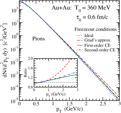
Figure 6.1: Pion spectra as a function of the transverse momentum $p_{T}$, obtained with the second-order hydrodynamic evolution, followed by freezeout in various scenarios: ideal, Grad’s 14-moment approximation, first- and second-order Chapman-Enskog. Inset: Pion yields in the above four cases scaled by the corresponding values in the ideal case.

We solve the evolution equations (6.18)-(6.19) with initial temperature $T_{0}=360$ MeV, time $\tau_{0}=0.6$ fm/$c$, and isotropic pressure configuration $\Phi_{0}=0$, corresponding to central ($b=0$) Au-Au collisions at the Relativistic Heavy-Ion Collider. The system is evolved with shear viscosity to entropy density ratio $\eta/s=1/4\pi$ corresponding to the KSS lower bound [Kovtun:2004de], until the freezeout temperature $T=150$ MeV is reached. In order to study the effects of the various forms of $\delta f$ via the freezeout prescription, Eq. (6.23), we evolve the system using the second-order viscous hydrodynamic equations (6.18) and (6.19) in all the cases.

In Fig. 6.1, we present the pion transverse-momentum spectra for the four freezeout conditions discussed above, namely ideal, first- and second-order Chapman-Enskog, and Grad’s 14-moment approximation. We observe that nonideal freezeout conditions tend to increase the high-$p_{T}$ particle production. While the Chapman-Enskog corrections are small, Grad’s 14-moment approximation results in rather large corrections to the ideal case. This is clearly evident in the inset where we show the pion yields in the four cases scaled by the values in the ideal case. These features can be easily understood from Eqs. (6.25) and (6.26): The first-order Chapman-Enskog correction is essentially linear in $p_{T}$ whereas that due to Grad is quadratic. The second-order Chapman-Enskog correction is small, indicating rapid convergence of the expansion up to second order.

6.8 HBT radii

HBT interferometry provides a powerful tool to unravel the space-time structure of the particle emitting sources in heavy-ion collisions, because of its ability to measure source sizes, lifetimes and particle emission durations [Lisa:2005dd]. The source function, $S(x,K)$ for on-shell particle emission is defined such that it satisfies

$$\frac{dN}{d^{2}K_{T}dy}\equiv\int d^{4}x\,S(x,K).$$ (6.27)

Comparing the above equation with Eq. (6.23), we see that the source function is restricted to the freezeout hypersurface and is given by

$$S(x,K)=\frac{g}{(2\pi)^{3}}\int p_{\mu}d\Sigma^{\mu}(x^{\prime})f(x^{\prime},p)\delta^{4}(x-x^{\prime}).$$ (6.28)

At relatively small momenta, certain space-time variances of the source function can be obtained, to a good approximation, from the correlation between particle pairs [Wiedemann:1999qn]. Space-time averages with respect to the source function are defined as

$$\left\langle\alpha\right\rangle_{K}\equiv\frac{\int d^{4}x\,S(x,K)\alpha}{\int d^{4}x\,S(x,K)}=\frac{\int K_{\mu}d\Sigma^{\mu}f(x,K)\alpha}{\int K_{\mu}d\Sigma^{\mu}f(x,K)},$$ (6.29)

where $K_{\mu}$ is the pair four-momentum.

The longitudinal HBT radius, $R_{L}$, is calculated in terms of the transverse momentum, $K_{T}$, of the identical-particle pair [Wiedemann:1999qn]:

$$R_{L}^{2}(K_{T})=\frac{\int K_{\mu}d\Sigma^{\mu}f(x,K)z^{2}}{\int K_{\mu}d\Sigma^{\mu}f(x,K)}.$$ (6.30)

In the central-rapidity region, the pair four momentum is given by $K^{\mu}=(K^{\tau},K^{r},K^{\varphi},K^{\eta_{s}})=(m_{T},K_{T},0,0)$. The integration measure is given by $K_{\mu}d\Sigma^{\mu}=m_{T}\cosh(\eta_{s})\tau d\eta_{s}rdrd\varphi$ with $m_{T}=\sqrt{K_{T}^{2}+m_{p}^{2}}$, $m_{p}$ being the particle mass. Using the relation $z=\tau\,\sinh(\eta_{s})$, we get

$$R_{L}^{2}(K_{T}) =\tau^{2}\left[\frac{\int K_{\mu}d\Sigma^{\mu}f(x,K){\cosh^{2}(\eta_{s})}}{\int K_{\mu}d\Sigma^{\mu}f(x,K)}-1\right],$$

$$\equiv\tau^{2}\left[\frac{N[f]}{D[f]}-1\right].$$ (6.31)

Note that the integral, $D[f]$, in the denominator in the above equation is the same as that occurring in the Cooper-Frye prescription for particle production, Eq. (6.23), and was already calculated in the previous section. We next calculate the integral, $N[f]$, in the numerator.

In the ideal case, $f=f_{0}$, we have

$$N[f_{0}]=\frac{2A_{\perp}\tau z_{m}}{4\beta}\left(K_{3}+3K_{1}\right).$$ (6.32)

This leads to the well known result of Hermann and Bertsch [Herrmann:1994rr]

$$(R_{L}^{2})^{(0)}=\frac{\tau^{2}}{z_{m}}\,\frac{K_{2}}{K_{1}},$$ (6.33)

which for large values of $z_{m}$ results in the Makhlin-Sinyukov formula $(R_{L}^{2})^{(0)}=\tau^{2}T/m_{T}$ [Makhlin:1987gm, Csorgo:1995bi]. Thus in the ideal case, $(R_{L})^{(0)}$ exhibits the so-called $1/\sqrt{m_{T}}$ scaling.

The first-order calculation requires $N[\delta f_{1}]$ which is given by

$$N[\delta f_{1}]=\frac{2A_{\perp}\tau\Phi}{16\beta\beta_{\pi}}\Big{[}\left(2z_{p}^{2}+z_{m}^{2}\right)K_{0}+2z_{p}^{2}K_{2}-z_{m}^{2}K_{4}\Big{]}.$$ (6.34)

The second-order calculation requires $N[\delta f_{2}]$ which is given in the Appendix C. For comparison we also calculate $R_{L}$ in Grad’s 14-moment approximation. This requires $N[\delta f_{G}]$, which we obtain as

$$N[\delta f_{G}]=\frac{2A_{\perp}\tau\Phi z_{m}}{160\beta\beta_{\pi}}\Big{[}\left(2z_{p}^{2}-6z_{m}^{2}\right)K_{1}+\left(2z_{p}^{2}-z_{m}^{2}\right)K_{3}-z_{m}^{2}K_{5}\Big{]}.$$ (6.35)

In the following, we show that the viscous correction to $R_{L}$ due to Grad’s 14-moment approximation violates the experimentally observed $1/\sqrt{m_{T}}$ scaling [Bearden:2001sy, Adcox:2002uc], whereas it is preserved in the Chapman-Enskog case. To this end, we calculate the first-order viscous correction to $R_{L}$ in both the cases. Expanding the $R_{L}$ in Eq. (6.30) to first order in $\delta f$ and using the relation $z=\tau\sinh(\eta_{s})$ we obtain the ideal contribution

$$(R_{L}^{2})^{(0)}= ~{}\frac{\int K^{\mu}d\Sigma_{\mu}\,f_{0}\,\tau^{2}\sinh^{2}(\eta_{s})}{\int K^{\mu}d\Sigma_{\mu}\,f_{0}},$$ (6.36)

and the first viscous correction in the two cases

$$\left(\delta R_{L}^{2}\right)^{(1,G)}=-(R_{L}^{2})^{(0)}\left(\frac{dN^{(1,G)}}{d^{2}K_{T}}-\frac{dN^{(0)}}{d^{2}K_{T}}\right)\!\!\Big{/}\frac{dN^{(0)}}{d^{2}K_{T}}+\frac{\int K^{\mu}d\Sigma_{\mu}\,\tau^{2}\sinh^{2}(\eta_{s})\,\delta f_{1,G}}{\int K^{\mu}d\Sigma_{\mu}\,f_{0}}.$$ (6.37)

The ideal radius $(R_{L}^{2})^{(0)}$ was obtained in Eq. (6.33). Viscous corrections due to the Chapman-Enskog method and Grad’s 14-moment approximation can be obtained similarly. Substituting the viscous correction, $\delta f_{1}$, from Eq. (6.13) into Eq. (6.37), using the results for the particle spectra, Eqs. (6.24), (6.25) and the ideal radius, Eq. (6.33), and performing the $\eta_{s}$ integrals, we obtain

$$\frac{\left(\delta R_{L}^{2}\right)^{(1)}}{\left(R_{L}^{2}\right)^{(0)}}=-\frac{\Phi}{16\beta_{\pi}}\left[16+\frac{4z_{p}^{2}}{z_{m}}\left(\frac{K_{0}}{K_{1}}-\frac{K_{1}}{K_{2}}\right)\right].$$ (6.38)

Similarly, for Grad’s approximation, Eq. (6.17), we obtain

$$\frac{\left(\delta R_{L}^{2}\right)^{(G)}}{\left(R_{L}^{2}\right)^{(0)}}=-\frac{\Phi}{20\beta_{\pi}}\left[20-2z_{m}\left(\frac{K_{0}}{K_{1}}-\frac{K_{1}}{K_{2}}\right)+4z_{m}\frac{K_{1}}{K_{2}}\right].$$ (6.39)

Using the asymptotic expansion of modified Bessel functions of the second kind [abramowitz],

$$K_{n}(z_{m})=\left(\frac{\pi}{2z_{m}}\right)^{\frac{1}{2}}e^{-z_{m}}\left[1+\frac{4n^{2}-1}{8z_{m}}+\cdots\right],$$ (6.40)

for large $z_{m}$, we have

$$\frac{K_{0}}{K_{1}}-\frac{K_{1}}{K_{2}}=\frac{1}{z_{m}}+{\mathcal{O}}\left(\frac{1}{z_{m}^{2}}\right).$$ (6.41)

Hence, for large values of $z_{m}$, we find

$$\left(\delta R_{L}^{2}\right)^{(1)} =-\frac{5\tau^{2}T\Phi}{4\beta_{\pi}m_{T}},$$ (6.42)

$$\left(\delta R_{L}^{2}\right)^{(G)} =-\frac{\tau^{2}T\Phi}{5\beta_{\pi}m_{T}}\left(3+\frac{m_{T}}{T}\right).$$ (6.43)

It is clear from the above two equations that the viscous correction to $R_{L}$ in the Chapman-Enskog case preserves the $1/\sqrt{m_{T}}$ scaling, whereas in Grad’s 14-moment approximation it grows as $m_{T}/T$, and thus violates the scaling [Teaney:2003kp].

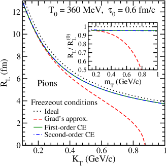
Figure 6.2: Longitudinal HBT radius as a function of the transverse momentum $K_{T}$ of the pion pair, obtained with the second-order hydrodynamic evolution, followed by freezeout in various scenarios: ideal, Grad’s 14-moment approximation, first- and second-order Chapman-Enskog. Inset: HBT radius in the above cases scaled by the corresponding values in the ideal case.

Results for the longitudinal HBT radius, $R_{L}$, for identical-pion pairs in central Au-Au collisions, for the four cases discussed above, are displayed in Fig. 6.2. We note that while there is no noticeable difference between first- and second-order Chapman-Enskog results compared to the ideal case, they predict a slightly smaller value for $R_{L}$. On the other hand, $R_{L}$ corresponding to Grad’s approximation exhibits a qualitatively different behaviour and even becomes imaginary for $K_{T}\gtrsim 0.9$ GeV/$c$, which is clearly unphysical. More importantly, the ratio $R_{L}/R_{L}^{(0)}$ shown in the inset of Fig. 6.2, illustrates that the $1/\sqrt{m_{T}}$ scaling which is violated in Grad’s approximation, survives in the Chapman-Enskog case.

6.9 Summary and Conclusions

We derived the form of the viscous correction to the equilibrium distribution function, up to second order in gradients, by employing a Chapman-Enskog-like iterative solution of the Boltzmann equation in the relaxation time approximation. This approach is in accordance with the formulation of hydrodynamics which is also a gradient expansion. We used this form of the viscous correction to calculate the hadronic transverse-momentum spectra and longitudinal Hanbury Brown-Twiss radii, and compared them with those obtained in Grad’s 14-moment approximation within the one-dimensional scaling expansion. These results demonstrate the rapid convergence of the Chapman-Enskog expansion up to second order, and thus it is sufficient to retain only the first-order correction in the freezeout prescription. We found that the Chapman-Enskog method results in softer hadron spectra compared with Grad’s approximation. We further showed that the experimentally observed $1/\sqrt{m_{T}}$ scaling of HBT radii which is also seen in the ideal freezeout calculation, is maintained in the Chapman-Enskog method. In contrast, the Grad’s 14-moment approximation leads to the violation of this scaling as well as an imaginary value for $R_{L}$ at large momenta. For initial conditions typical of heavy-ion collisions at the Large Hadron Collider ($T_{0}=500$ MeV and $\tau_{0}=0.4$ fm/$c$), we have found that the above conclusions remain unchanged.

Unlike Grad’s approximation which is linear in dissipative quantities, the form of viscous correction to the distribution function obtained here using Chapman-Enskog like expansion contains higher-order nonlinear corrections to the equilibrium distribution function. This has important implications for the formulation of dissipative hydrodynamics as an order-by-order expansion in gradients. For example, by calculating the nonequilibrium distribution function to any given order, the dissipative evolution equation up to that order can be derived. In the next chapter, we present the derivation of a novel third-order hydrodynamic evolution equation for shear stress tensor from kinetic theory and quantify the significance of this new derivation within one-dimensional scaling expansion.

We conclude by recalling the well-known form of the viscous correction due to Grad’s 14-moment approximation:

$$\delta f_{G}=\frac{f_{0}\tilde{f}_{0}}{2(\epsilon+P)T^{2}}\,p^{\alpha}p^{\beta}\pi_{\alpha\beta},$$ (6.44)

and the alternate form due to Chapman-Enskog method proposed here:

$$\delta f_{CE}=\frac{5f_{0}\tilde{f}_{0}}{8PT(u\!\cdot\!p)}\,p^{\alpha}p^{\beta}\pi_{\alpha\beta},$$ (6.45)

where $\tilde{f}_{0}\equiv 1-rf_{0}$, with $r=1,-1,0$ for Fermi, Bose, and Boltzmann gases, respectively. In view of the arguments presented in this chapter, we advocate that the form of $\delta f_{CE}$ proposed here should be a better alternative for hydrodynamic modelling of relativistic heavy-ion collisions.

Chapter 7 Relativistic third-order viscous fluid dynamics from kinetic theory

7.1 Introduction

Despite the success of IS theory in explaining a wide range of collective phenomena observed in heavy-ion collisions, its formulation is based on strong assumptions and approximations. The original IS theory derived from Boltzmann equation (BE) uses two powerful assumptions in the derivation of dissipative equations: use of second moment of BE and the 14-moment approximation [Israel:1979wp, Grad]. In Ref. [Denicol:2010xn], although the dissipative equations were derived directly from their definitions without resorting to second-moment of BE, however the 14-moment approximation was still employed. In Chapter 5, it was shown that both these assumptions are unnecessary, and instead of 14-moment approximation, iterative solution of BE was used to obtain the dissipative evolution equations from their definitions.

Apart from these problems in the formulation, IS theory suffers from several other shortcomings. In one-dimensional Bjorken scaling expansion [Bjorken:1982qr], for large viscosities or small initial time, IS theory has resulted in unphysical effects such as reheating of the expanding medium [Muronga:2003ta] and negative longitudinal pressure [Martinez:2009mf]. Further, the scaling solutions of IS equations when compared with transport results show disagreement for $\eta/s>0.5$ indicating the breakdown of second-order theory [Huovinen:2008te, El:2008yy]. With this motivation, in Ref. [Jaiswal:2012qm], second-order dissipative equations were derived from BE where the collision term was generalized to include nonlocal effects via gradients of the distribution function. Moreover, in Refs. [Jaiswal:2013npa, El:2009vj] it was demonstrated that a heuristic inclusion of higher-order corrections led to an improved agreement with transport results. In fact, the derivation of higher-order constitutive equations from kinetic theory for non-relativistic systems has been known for a long time [Cha]. Thus it is of interest to improvise the relativistic second-order theory by incorporating higher-order corrections.

In this chapter, we derive a new relativistic third-order evolution equation for shear stress tensor from kinetic theory. Without resorting to the widely used Grad’s 14-moment approximation [Grad], we iteratively solve the BE in relaxation time approximation (RTA) to obtain nonequilibrium phase-space distribution function. We subsequently derive equation of motion for shear stress tensor up-to third-order, directly from its definition. Within one-dimensional scaling expansion, the results obtained using third-order evolution equations derived here shows improved agreement with exact solution of BE as compared to second-order equations. We also demonstrate that the evolution of pressure anisotropy obtained using our equations shows better agreement with the transport results as compared to those obtained by using an existing third-order equation derived from entropy considerations.

7.2 Relativistic hydrodynamics

The hydrodynamic evolution of a system is governed by the conservation equations for energy and momentum. The conserved energy-momentum tensor can be expressed in terms of single-particle, phase-space distribution function and tensor decomposed into hydrodynamic variables [deGroot]. For a system of massless particles, bulk viscosity vanishes leading to

$$T^{\mu\nu} =\!\int\!dp\ p^{\mu}p^{\nu}\,f(x,p)=\epsilon u^{\mu}u^{\nu}-P\Delta^{\mu\nu}+\pi^{\mu\nu},$$ (7.1)

where $dp\equiv gd{\bf p}/[(2\pi)^{3}|\bf p|]$, $g$ being the degeneracy factor, $p^{\mu}$ is the particle four-momentum and $f(x,p)$ is the phase-space distribution function. In the tensor decompositions, $\epsilon$, $P$ and $\pi^{\mu\nu}$ are respectively energy density, pressure and the shear stress tensor. The projection operator $\Delta^{\mu\nu}\equiv g^{\mu\nu}-u^{\mu}u^{\nu}$ is orthogonal to the hydrodynamic four-velocity $u^{\mu}$ defined in the Landau frame: $T^{\mu\nu}u_{\nu}=\epsilon u^{\mu}$. The metric tensor is Minkowskian, $g^{\mu\nu}\equiv\mathrm{diag}(+,-,-,-)$.

Energy-momentum conservation, $\partial_{\mu}T^{\mu\nu}=0$ yields the fundamental evolution equations for $\epsilon$ and $u^{\mu}$

$$\dot{\epsilon}+(\epsilon+P)\theta-\pi^{\mu\nu}\nabla_{(\mu}u_{\nu)} =0,$$

$$(\epsilon+P)\dot{u}^{\alpha}-\nabla^{\alpha}P+\Delta^{\alpha}_{\nu}\partial_{\mu}\pi^{\mu\nu} =0.$$ (7.2)

As in the previous chapters, we use the notation $\dot{A}\equiv u^{\mu}\partial_{\mu}A$ for comoving derivative, $\theta\equiv\partial_{\mu}u^{\mu}$ for the expansion scalar, $A^{(\alpha}B^{\beta)}\equiv(A^{\alpha}B^{\beta}+A^{\beta}B^{\alpha})/2$ for symmetrization and $\nabla^{\alpha}\equiv\Delta^{\mu\alpha}\partial_{\mu}$ for space-like derivative. In the massless limit, the energy density and pressure are related as $\epsilon=3P\propto\beta^{-4}$. The inverse temperature, $\beta\equiv 1/T$, is defined by the Landau matching condition $\epsilon=\epsilon_{0}$ where $\epsilon_{0}$ is the equilibrium energy density. In this limit, Eqs. (7.2) can be used to obtain the derivatives of $\beta$ as

$$\dot{\beta}=\frac{\beta}{3}\theta-\frac{\beta}{12P}\pi^{\rho\gamma}\sigma_{\rho\gamma},\quad\nabla^{\alpha}\beta=\!-\beta\dot{u}^{\alpha}-\frac{\beta}{4P}\Delta^{\alpha}_{\rho}\partial_{\gamma}\pi^{\rho\gamma},$$ (7.3)

where $\sigma^{\rho\gamma}\equiv\nabla^{(\rho}u^{\gamma)}-(\theta/3)\Delta^{\rho\gamma}$ is the velocity stress tensor. The above identities will be helpful in the derivation of shear evolution equation.

The expression for shear stress tensor ($\pi^{\mu\nu}$) can be obtained in terms of the out-of-equilibrium part of the distribution function. To this end, we write the nonequilibrium distribution function as $f=f_{0}+\delta f$, where the deviation from equilibrium is assumed to be small $(\delta f\ll f)$. The equilibrium distribution function represents Boltzmann statistics of massless particles at vanishing chemical potential, $f_{0}=\exp(-\beta\,u\cdot p)$, where $u\cdot p\equiv u_{\mu}p^{\mu}$. From Eq. (7.1), $\pi^{\mu\nu}$ can be expressed in terms of $\delta f$ as

$$\pi^{\mu\nu} =\Delta^{\mu\nu}_{\alpha\beta}\int dp\,p^{\alpha}p^{\beta}\,\delta f,$$ (7.4)

where $\Delta^{\mu\nu}_{\alpha\beta}\equiv\Delta^{\mu}_{(\alpha}\Delta^{\nu}_{\beta)}-(1/3)\Delta^{\mu\nu}\Delta_{\alpha\beta}$ is a traceless symmetric projection operator orthogonal to $u^{\mu}$. To proceed further, the form of $\delta f$ has to be specified. In the following, Boltzmann equation in RTA will be solved iteratively to obtain $\delta f$ order-by-order in gradients.

7.3 Chapman-Enskog expansion

As demonstrated in the previous chapters, nonequilibrium phase-space distribution function can be obtained by solving the one-body kinetic equation such as the Boltzmann equation. The most common technique of generating solutions to such equations is the Chapman-Enskog expansion where the particle distribution function is expanded about its equilibrium value in powers of space-time gradients [Chapman], which we repeat for convenience.

$$f=f_{0}+\delta f,\quad\delta f=\delta f^{(1)}+\delta f^{(2)}+\cdots,$$ (7.5)

where $\delta f^{(1)}$ is first-order in derivatives, $\delta f^{(2)}$ is second-order and so on. Subsequently, the relativistic Boltzmann equation with relaxation time approximation for the collision term [Anderson_Witting],

$$p^{\mu}\partial_{\mu}f=-u\!\cdot\!p\frac{\delta f}{\tau_{R}}\;\Rightarrow\;f=f_{0}-(\tau_{R}/u\!\cdot\!p)\,p^{\mu}\partial_{\mu}f,$$ (7.6)

can be solved iteratively as [Jaiswal:2013npa, Romatschke:2011qp]

$$f_{1}=f_{0}-\frac{\tau_{R}}{u\!\cdot\!p}\,p^{\mu}\partial_{\mu}f_{0},\quad f_{2}=f_{0}-\frac{\tau_{R}}{u\!\cdot\!p}\,p^{\mu}\partial_{\mu}f_{1},\quad\cdots$$ (7.7)

where $f_{n}=f_{0}+\delta f^{(1)}+\delta f^{(2)}+\cdots+\delta f^{(n)}$. To first and second-order in derivatives, we obtain

$$\delta f^{(1)}=-\frac{\tau_{R}}{u\!\cdot\!p}\,p^{\mu}\partial_{\mu}f_{0},\quad\delta f^{(2)}=\frac{\tau_{R}}{u\!\cdot\!p}p^{\mu}p^{\nu}\partial_{\mu}\Big{(}\frac{\tau_{R}}{u\!\cdot\!p}\partial_{\nu}f_{0}\Big{)}.$$ (7.8)

The above expressions for nonequilibrium part of the distribution function along with Eq. (7.4) will be used in the derivation of shear evolution equations.

As a side remark, note that the RTA for the collision term, $C[f]=-(u\cdot p)\delta f/\tau_{R}$ in Eq. (7.6), should satisfy current and energy-momentum conservation, i.e., the zeroth and first moment of the collision term should vanish [deGroot]. Assuming the relaxation time $\tau_{R}$ to be independent of momenta, these conservation equations are satisfied only if the fluid four-velocity is defined in the Landau frame [Anderson_Witting]. Hence, within RTA, the Landau frame is imposed and is not a choice.

7.4 Evolution equations for shear stress tensor

The first-order expression for shear stress tensor can be obtained from Eq. (7.4) using $\delta f=\delta f^{(1)}$ from Eq. (7.8),

$$\pi^{\mu\nu} =\Delta^{\mu\nu}_{\alpha\beta}\int dp\ p^{\alpha}p^{\beta}\left(-\frac{\tau_{R}}{u\!\cdot\!p}\,p^{\mu}\partial_{\mu}\,f_{0}\right).$$ (7.9)

Using Eqs. (7.3) and keeping only those terms which are first-order in gradients, the integrals in the above equation reduce to

$$\pi^{\mu\nu}=2\tau_{R}\beta_{\pi}\sigma^{\mu\nu},\quad\beta_{\pi}=\frac{4}{5}P.$$ (7.10)

To obtain the second-order evolution equation, we follow the methodology discussed in Ref. [Denicol:2010xn]. The evolution of the shear stress tensor can be obtained by considering the comoving derivative of Eq. (7.4),

$$\dot{\pi}^{\langle\mu\nu\rangle}=\Delta^{\mu\nu}_{\alpha\beta}\int dp\,p^{\alpha}p^{\beta}\,\delta\dot{f},$$ (7.11)

where the notation $A^{\langle\mu\nu\rangle}\equiv\Delta^{\mu\nu}_{\alpha\beta}A^{\alpha\beta}$ represents traceless symmetric projection orthogonal to $u^{\mu}$.

The comoving derivative of the nonequilibrium part of the distribution function ($\delta\dot{f}$) can be obtained by rewriting Eq. (7.6) in the form

$$\delta\dot{f}=-\dot{f}_{0}-\frac{1}{u\!\cdot\!p}p^{\gamma}\nabla_{\gamma}f-\frac{\delta f}{\tau_{R}},$$ (7.12)

Using this expression for $\delta\dot{f}$ in Eq. (7.11), we obtain

$$\dot{\pi}^{\langle\mu\nu\rangle}+\frac{\pi^{\mu\nu}}{\tau_{R}}=-\Delta^{\mu\nu}_{\alpha\beta}\!\int\!dp\,p^{\alpha}p^{\beta}\!\left(\dot{f}_{0}+\frac{1}{u\!\cdot\!p}p^{\gamma}\nabla_{\gamma}f\right)\!.$$ (7.13)

It is clear that in the above equation, the Boltzmann relaxation time $\tau_{R}$ can be replaced by the shear relaxation time $\tau_{\pi}$. By comparing the first-order evolution Eq. (7.10) with the relativistic Navier-Stokes equation $\pi^{\mu\nu}=2\eta\sigma^{\mu\nu}$, the shear relaxation time is obtained in terms of the first-order transport coefficient, $\tau_{\pi}=\eta/\beta_{\pi}$.

Note that for the shear evolution equations to be second-order in gradients, the distribution function on the right hand side of Eq. (7.13) need to be computed only till first-order, i.e., $f=f_{1}=f_{0}+\delta f^{(1)}$. Using Eq. (7.8) for $\delta f^{(1)}$ and Eqs. (7.3) for derivatives of $\beta$, and keeping terms up to quadratic order in gradients, the second-order shear evolution equation is obtained as [Jaiswal:2013npa]

$$\dot{\pi}^{\langle\mu\nu\rangle}\!+\frac{\pi^{\mu\nu}}{\tau_{\pi}}\!=2\beta_{\pi}\sigma^{\mu\nu}\!+2\pi_{\gamma}^{\langle\mu}\omega^{\nu\rangle\gamma}\!-\frac{10}{7}\pi_{\gamma}^{\langle\mu}\sigma^{\nu\rangle\gamma}\!-\frac{4}{3}\pi^{\mu\nu}\theta,$$ (7.14)

where $\omega^{\mu\nu}\equiv(\nabla^{\mu}u^{\nu}-\nabla^{\nu}u^{\mu})/2$ is the vorticity tensor. We have used the first-order expression for shear stress tensor, Eq. (7.10), to replace $\sigma^{\mu\nu}\to\pi^{\mu\nu}$ such that the relaxation times appearing on the right hand side of Eq. (7.13) are absorbed.

To derive a third-order evolution equation for shear stress tensor, the distribution function on the right hand side of Eq. (7.13) needs to be computed till second-order ($\delta f=\delta f^{(1)}+\delta f^{(2)}$). In order to account for all the higher-order terms, Eq. (7.14) was used to substitute for $\sigma^{\mu\nu}$. Employing Eqs. (7.3) for derivatives of $\beta$ and keeping terms up to cubic order in derivatives, we finally obtain a unique third-order evolution equation for shear stress tensor after a straightforward but tedious algebra

$$\dot{\pi}^{\langle\mu\nu\rangle}= -\frac{\pi^{\mu\nu}}{\tau_{\pi}}+2\beta_{\pi}\sigma^{\mu\nu}+2\pi_{\gamma}^{\langle\mu}\omega^{\nu\rangle\gamma}-\frac{10}{7}\pi_{\gamma}^{\langle\mu}\sigma^{\nu\rangle\gamma}-\frac{4}{3}\pi^{\mu\nu}\theta+\frac{25}{7\beta_{\pi}}\pi^{\rho\langle\mu}\omega^{\nu\rangle\gamma}\pi_{\rho\gamma}-\frac{1}{3\beta_{\pi}}\pi_{\gamma}^{\langle\mu}\pi^{\nu\rangle\gamma}\theta$$

$$-\frac{38}{245\beta_{\pi}}\pi^{\mu\nu}\pi^{\rho\gamma}\sigma_{\rho\gamma}-\frac{22}{49\beta_{\pi}}\pi^{\rho\langle\mu}\pi^{\nu\rangle\gamma}\sigma_{\rho\gamma}-\frac{24}{35}\nabla^{\langle\mu}\left(\pi^{\nu\rangle\gamma}\dot{u}_{\gamma}\tau_{\pi}\right)+\frac{4}{35}\nabla^{\langle\mu}\left(\tau_{\pi}\nabla_{\gamma}\pi^{\nu\rangle\gamma}\right)$$

$$-\frac{2}{7}\nabla_{\gamma}\left(\tau_{\pi}\nabla^{\langle\mu}\pi^{\nu\rangle\gamma}\right)+\frac{12}{7}\nabla_{\gamma}\left(\tau_{\pi}\dot{u}^{\langle\mu}\pi^{\nu\rangle\gamma}\right)-\frac{1}{7}\nabla_{\gamma}\left(\tau_{\pi}\nabla^{\gamma}\pi^{\langle\mu\nu\rangle}\right)+\frac{6}{7}\nabla_{\gamma}\left(\tau_{\pi}\dot{u}^{\gamma}\pi^{\langle\mu\nu\rangle}\right)$$

$$-\frac{2}{7}\tau_{\pi}\omega^{\rho\langle\mu}\omega^{\nu\rangle\gamma}\pi_{\rho\gamma}-\frac{2}{7}\tau_{\pi}\pi^{\rho\langle\mu}\omega^{\nu\rangle\gamma}\omega_{\rho\gamma}-\frac{10}{63}\tau_{\pi}\pi^{\mu\nu}\theta^{2}+\frac{26}{21}\tau_{\pi}\pi_{\gamma}^{\langle\mu}\omega^{\nu\rangle\gamma}\theta.$$ (7.15)

The above equation constitutes the main result of this chapter. We note that Eq. (7.4) represents only a subset of all possible third order terms because bulk viscosity and heat current has been neglected.

We compare the third-order shear evolution equation derived here with that obtained by El et al., in Ref. [El:2009vj]. In the latter work, the shear evolution equation was derived by invoking second law of thermodynamics from kinetic definition of entropy four-current, expanded till third-order in $\pi^{\mu\nu}$. For ease of comparison, we write the evolution equation obtained in Ref. [El:2009vj] in the form

$$\dot{\pi}^{\langle\mu\nu\rangle}=-\frac{\pi^{\mu\nu}}{\tau_{\pi}^{\prime}}+2\beta_{\pi}^{\prime}\sigma^{\mu\nu}-\frac{4}{3}\pi^{\mu\nu}\theta+\frac{5}{36\beta_{\pi}^{\prime}}\pi^{\mu\nu}\pi^{\rho\gamma}\sigma_{\rho\gamma}-\frac{16}{9\beta_{\pi}^{\prime}}\pi^{\langle\mu}_{\gamma}\pi^{\nu\rangle\gamma}\theta,$$ (7.16)

where $\beta_{\pi}^{\prime}=2P/3$ and $\tau_{\pi}^{\prime}=\eta/\beta_{\pi}^{\prime}$. We observe that the right-hand-side of Eq. (7.16) contains one second-order and two third-order terms compared to three second-order and fourteen third-order terms obtained here, i.e., Eq. (7.4). It is well known that the approach based on entropy method fails to capture all the terms in the dissipative evolution equations even at second-order. Moreover, the discrepancy at third-order confirms the fact that the evolution equation obtained by invoking second law of thermodynamics is incomplete.

7.5 Numerical results and discussion

To demonstrate the numerical significance of the third-order shear evolution equation derived here, we consider boost-invariant Bjorken expansion of a system consisting of massless Boltzmann gas [Bjorken:1982qr]. Working in Milne coordinates $(\tau,x,y,\eta_{s})$, where $\tau=\sqrt{t^{2}-z^{2}}$, $\eta_{s}=\tanh^{-1}(z/t)$, and with $u^{\mu}=(1,0,0,0)$, we observe that only the $\eta_{s}\eta_{s}$ component of Eq. (7.4) survives. In this scenario, $\omega^{\mu\nu}=\dot{u}^{\mu}=\nabla^{\mu}\tau_{\pi}=0$, $\theta=1/\tau$ and $\sigma^{\eta_{s}\eta_{s}}=-2/(3\tau^{3})$. Defining $\Phi\equiv-\tau^{2}\pi^{\eta_{s}\eta_{s}}$, we find that $\pi^{\rho\gamma}\sigma_{\rho\gamma}=\Phi/\tau$, and

$$\dot{\pi}^{\langle\eta_{s}\eta_{s}\rangle}=-\frac{1}{\tau^{2}}\frac{d\Phi}{d\tau},\quad\pi^{\langle\eta_{s}}_{\gamma}\sigma^{\eta_{s}\rangle\gamma}=-\frac{\Phi}{3\tau^{3}},\quad\pi^{\langle\eta_{s}}_{\gamma}\pi^{\eta_{s}\rangle\gamma}=-\frac{\Phi^{2}}{2\tau^{2}},\quad\pi^{\rho\langle\eta_{s}}\pi^{\eta_{s}\rangle\gamma}\sigma_{\rho\gamma}=-\frac{\Phi^{2}}{2\tau^{3}},$$

$$\nabla^{\langle\eta_{s}}\nabla_{\gamma}\pi^{\eta_{s}\rangle\gamma}=\frac{2\Phi}{3\tau^{4}},\quad\nabla_{\gamma}\nabla^{\langle\eta_{s}}\pi^{\eta_{s}\rangle\gamma}=\frac{4\Phi}{3\tau^{4}},\quad\nabla^{2}\pi^{\langle\eta_{s}\eta_{s}\rangle}=\frac{4\Phi}{3\tau^{4}},$$ (7.17)

see Appendix A for details. Using the above results, evolution of $\epsilon$ and $\Phi$ from Eqs. (7.2) and (7.4) reduces to

$$\frac{d\epsilon}{d\tau} =-\frac{1}{\tau}\left(\epsilon+P-\Phi\right),$$ (7.18)

$$\frac{d\Phi}{d\tau} =-\frac{\Phi}{\tau_{\pi}}+\beta_{\pi}\frac{4}{3\tau}-\lambda\frac{\Phi}{\tau}-\chi\frac{\Phi^{2}}{\beta_{\pi}\tau}.$$ (7.19)

The term with coefficient $\chi$ in the above equation contains correction only due to third-order. The first-order shear expression, $\Phi=4\beta_{\pi}\tau_{\pi}/3\tau$, has been used to rewrite some of the third-order contributions in the form $\Phi^{2}/(\beta_{\pi}\tau)$. The transport coefficients in our calculation simplify to

$$\tau_{\pi}=\frac{\eta}{\beta_{\pi}},\quad\beta_{\pi}=\frac{4P}{5},\quad\lambda=\frac{38}{21},\quad\chi=\frac{72}{245}.$$ (7.20)

We compare these transport coefficients with those obtained from Eq. (7.16), where they reduce to

$$\tau_{\pi}^{\prime}=\frac{\eta}{\beta_{\pi}^{\prime}},\quad\beta_{\pi}^{\prime}=\frac{2P}{3},\quad\lambda^{\prime}=\frac{4}{3},\quad\chi^{\prime}=\frac{3}{4}.$$ (7.21)

For comparison, we also state the exact solution of Eq. (7.6) in one-dimensional scaling expansion [Baym:1984np, Florkowski:2013lza]:

$$f(\tau)=D(\tau,\tau_{0})f_{\rm in}+\int_{\tau_{0}}^{\tau}\frac{d\tau^{\prime}}{\tau_{R}(\tau^{\prime})}D(\tau,\tau^{\prime})f_{0}(\tau^{\prime}),$$ (7.22)

where, $f_{\rm in}$ and $\tau_{0}$ are the initial distribution function and proper time respectively, and

$$D(\tau_{2},\tau_{1})=\exp\left[-\int_{\tau_{1}}^{\tau_{2}}\frac{d\tau^{\prime\prime}}{\tau_{R}(\tau^{\prime\prime})}\right].$$ (7.23)

The damping function $D(\tau_{2},\tau_{1})$ has the following properties:

$$D(\tau,\tau)=1,\quad D(\tau_{3},\tau_{2})D(\tau_{2},\tau_{1})=D(\tau_{3},\tau_{1}),\quad\frac{\partial D(\tau_{2},\tau_{1})}{\partial\tau_{2}}=-\frac{D(\tau_{2},\tau_{1})}{\tau_{R}(\tau_{2})}.$$ (7.24)

To obtain the exact solution, the Boltzmann relaxation time is taken to be the same as the shear relaxation time $(\tau_{R}=\tau_{\pi})$. The hydrodynamic quantities can then be calculated by using Eq. (7.22) for the distribution function in Eq. (7.1) and performing the integrations numerically.

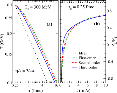
Figure 7.1: Time evolution of (a) temperature and (b) pressure anisotropy ($P_{L}/P_{T}$), in ideal (dotted line), first-order (dashed-dotted lines), second-order (dashed line) and third-order (solid lines) hydrodynamics, for Navier-Stokes initial condition, $(\Phi_{0}=4\eta/3\tau_{0})$.

To quantify the differences between ideal, first-order, second-order, and third-order theories, we solve the evolution equations with initial temperature $T_{0}=300$ MeV at initial time $\tau_{0}=0.25$ fm/c. These values correspond to the Relativistic Heavy-Ion Collider initial conditions [El:2007vg]. Figure 7.1 shows proper time evolution of temperature and pressure anisotropy $P_{L}/P_{T}\equiv(P-\Phi)/(P+\Phi/2)$ in ideal (dotted line), first-order (dashed-dotted lines), second-order (dashed line) and third-order (solid lines) hydrodynamics. Here we have assumed Navier-Stokes initial condition for shear pressure $(\Phi_{0}=4\eta/3\tau_{0})$ and solved the evolution equations for a representative shear viscosity to entropy density ratio, $\eta/s=3/4\pi$.

In Fig. 7.1 (a), we observe that while ideal hydrodynamics predicts a rapid cooling of the system, evolution based on third-order equation also shows faster temperature drop compared to first-order and second-order evolutions. This implies that the thermal photon and dilepton spectra, which are sensitive to temperature evolution, may be suppressed by including third-order corrections. Moreover, with third-order evolution, the freeze-out temperature is attained at an earlier time which may affect the hadronic spectra as well. In Fig. 7.1 (b), note that at early times the third-order evolution results in faster isotropization of pressure anisotropy compared to first-order and second-order. However at later time, the pressure anisotropy obtained using second and third-order equations merge indicating the convergence of gradient expansion in fluid dynamics.

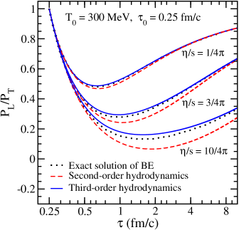
Figure 7.2: Time evolution of $P_{L}/P_{T}$ obtained using exact solution of Boltzmann equation (dotted line), second-order equations (dashed lines), and third-order equations (solid lines), for isotropic initial pressure configuration $(\Phi_{0}=0)$ and various $\eta/s$.

Figure 7.2, shows the proper time dependence of pressure anisotropy for various $\eta/s$ values with isotropic initial pressure configuration, i.e., $\Phi_{0}=0$. The improved agreement of third-order results (solid lines) with the exact solution of BE (dotted line) as compared to second-order results (dashed line) also suggests the convergence of the derivative expansion in hydrodynamics.

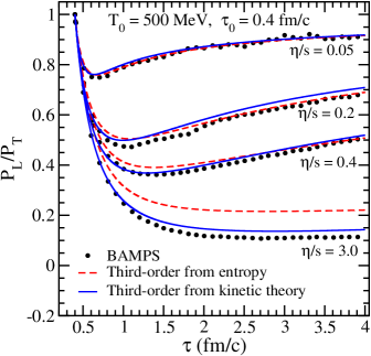
Figure 7.3: Time evolution of $P_{L}/P_{T}$ in BAMPS (dots), third-order calculation from entropy method, Eq. (7.16) (dashed lines), and the present work (solid lines), for isotropic initial pressure configuration $(\Phi_{0}=0)$ and various $\eta/s$.

Figure 7.3, also shows the time evolution of pressure anisotropy for initial temperature $T_{0}=500$ MeV at initial time $\tau_{0}=0.4$ fm/c which corresponds to Large Hadron Collider initial conditions [El:2007vg]. The initial pressure configuration is assumed to be isotropic and the evolution is shown for various $\eta/s$ values. The solid lines represent the results obtained in the present work by solving Eqs. (7.18) and (7.19) with transport coefficients of Eq. (7.20). The dashed lines corresponds to results of another third-order theory derived based on second-law of thermodynamics with transport coefficients given in Eq. (7.21). The dots represent the results of numerical solution of BE using a transport model, the parton cascade BAMPS [El:2009vj, Xu:2004mz]. The calculations in BAMPS are performed by changing the cross section such that $\eta/s$ remains constant. While the results from entropy derivation overestimate the pressure anisotropy for $\eta/s>0.2$, those obtained in the present work (kinetic theory) are in better agreement with the BAMPS results.

The RTA for the collision term in BE is based on the assumption that the effect of the collisions is to exponentially restore the distribution function to its local equilibrium value. Although the information about the microscopic interactions of the constituent particles is not retained here, it is a reasonably good approximation to describe a system which is close to local equilibrium. It is important to note that although the third-order viscous equations derived here uses BE with RTA for the collision term, the evolution shows good quantitative agreement with BAMPS results which employs realistic collision kernel [Xu:2004mz]. Indeed in Ref. [Dusling:2009df], it has been shown that for a purely gluonic system at weak coupling and hadron gas with large momenta, BE in RTA is a fairly accurate description. Furthermore, the experimentally observed $1/\sqrt{m_{T}}$ scaling of the HBT radii, which was shown to be broken by including viscous corrections to the distribution function [Teaney:2003kp], can be restored by using the form of the non-equilibrium distribution function obtained here [Bhalerao:2013pza]. All these factors clearly suggests that the BE in RTA can be applied quite successfully in understanding the hydrodynamic behaviour of the strongly interacting matter formed in heavy-ion collisions.

7.6 Summary and conclusions

To summarize, we have derived a novel third-order evolution equation for the shear stress tensor from kinetic theory within relaxation time approximation. Instead of Grad’s 14-moment approximation, iterative solution of Boltzmann equation was used for the nonequilibrium distribution function and the evolution equation for shear tensor is derived directly from its definition. Within one-dimensional scaling expansion, we have demonstrated that the third-order hydrodynamics derived here provides a very good approximation to the exact solution of Boltzmann equation in relaxation time approximation. Our results also show a better agreement with the parton cascade BAMPS for the $P_{L}/P_{T}$ evolution compared to those obtained from entropy derivation.

As discussed previously, the approach based on the generalized second law of thermodynamics fails to capture all the terms in the evolution equations of the dissipative quantities when compared with similar equations derived from kinetic theory. However, derivation of dissipative evolution equations from kinetic theory also fails to capture all the terms allowed by symmetry up to a given order in derivatives. Starting with the relativistic Boltzmann equation where the collision term is generalized to include nonlocal effects via gradients of the phase-space distribution function, and using Grad’s 14-moment approximation for the distribution function, we derive second-order evolution equations for relativistic dissipative fluids in the next chapter. Our method generates all the second-order terms that are allowed by symmetry, some of which have been missed by the traditional approaches based on the Boltzmann equation with local collision term.

Chapter 8 Nonlocal generalization of collision term and dissipative fluid dynamics

8.1 Introduction

The second-order viscous hydrodynamics has been quite successful in explaining the spectra and azimuthal anisotropy of particles produced in heavy-ion collisions at the Relativistic Heavy Ion Collider (RHIC) [Romatschke:2007mq, Song:2010mg] and recently at the Large Hadron Collider (LHC) [Luzum:2010ag, Qiu:2011hf]. However, IS theory can lead to unphysical effects such as reheating of the expanding medium [Muronga:2003ta] and to a negative pressure [Martinez:2009mf] at large viscosity indicating its breakdown. Furthermore, from comparison to the transport theory it was demonstrated [Huovinen:2008te, El:2008yy] that IS approach becomes marginal when the shear viscosity to entropy density ratio $\eta/s\gtrsim 1.5/(4\pi)$. With this motivation, the dissipative hydrodynamic equations were extended [El:2009vj, Jaiswal:2013vta, Jaiswal:2014raa] to third order, which led to an improved agreement with the kinetic theory even for moderately large values of $\eta/s$.

While it is well known that the approach based on the generalized second law of thermodynamics fails to capture several terms in the evolution equations of the dissipative quantities when compared with similar equations derived from transport theory [Baier:2006um], the derivation from kinetic theory also fails to capture all the terms allowed by symmetry. It was pointed out that using directly the definitions of the dissipative currents, instead of the second moment of the Boltzmann equation as in IS theory, one obtains identical equations of motion but with different coefficients [Denicol:2010xn]. Recently, it has been shown [Denicol:2012cn] that a generalization of Grad’s 14-moment method [Grad] results in additional terms in the dissipative equations.

It is important to note that all formulations that employ the Boltzmann equation make a strict assumption of a local collision term in the configuration space [Israel:1979wp, Denicol:2010xn]. In other words, within an infinitesimal fluid element containing a large number of particles and extending over many interparticle spacings [Landau], the different collisions that increase or decrease the number of particles with a given momentum $p$ are all assumed to occur at the same point $x^{\mu}$. This makes the collision integral a purely local functional of the single-particle phase-space distribution function $f(x,p)$ independent of the derivatives $\partial_{\mu}f(x,p)$. In kinetic theory, $f(x,p)$ is assumed to vary slowly over space-time, i.e., it changes negligibly over the range of interparticle interaction [deGroot]. However, its variation over the fluid element may not be insignificant; see Fig. 8.1. Inclusion of the gradients of $f(x,p)$ in the collision term will affect the evolution of dissipative quantities and thus the entire dynamics of the system.

In this chapter, we shall provide a new formal derivation of the dissipative hydrodynamic equations within kinetic theory but using a nonlocal collision term in the Boltzmann equation. We obtain new second-order terms and show that the coefficients of the other terms are altered. These modifications do have a rather strong influence on the evolution of the viscous medium as we shall demonstrate in the case of one-dimensional scaling expansion.

8.2 Nonlocal collision term

Our starting point is the relativistic Boltzmann equation for the evolution of the phase-space distribution function, $p^{\mu}\partial_{\mu}f=C[f]$, where the collision term $C[f]$ is required to be consistent with the energy-momentum and current conservation. Traditionally $C[f]$ is also assumed to be a purely local functional of $f(x,p)$, independent of $\partial_{\mu}f$. This locality assumption is a powerful restriction [Israel:1979wp] which we relax by including the gradients of $f(x,p)$ in $C[f]$. This necessarily leads to the modified Boltzmann equation

$$p^{\mu}\partial_{\mu}f=C_{m}[f]=C[f]+\partial_{\mu}(A^{\mu}f)+\partial_{\mu}\partial_{\nu}(B^{\mu\nu}f)+\cdots,$$ (8.1)

where $A^{\mu}$ and $B^{\mu\nu}$ depend on the type of the collisions ($2\leftrightarrow 2,~{}2\leftrightarrow 3,\ldots$).

For instance, for $2\leftrightarrow 2$ elastic collisions,

$$C[f]=\frac{1}{2}\int dp^{\prime}dk\ dk^{\prime}\ W_{pp^{\prime}\to kk^{\prime}}(f_{k}f_{k^{\prime}}\tilde{f}_{p}\tilde{f}_{p^{\prime}}-f_{p}f_{p^{\prime}}\tilde{f}_{k}\tilde{f}_{k^{\prime}}),$$ (8.2)

where $W_{pp^{\prime}\to kk^{\prime}}$ is the collisional transition rate, $f_{p}\equiv f(x,p)$ and $\tilde{f}_{p}\equiv 1-rf(x,p)$ with $r=1,-1,0$ for Fermi, Bose, and Boltzmann gas, and $dp=gd{\bf p}/[(2\pi)^{3}\sqrt{{\bf p}^{2}+m^{2}}]$, $g$ and $m$ being the degeneracy factor and particle rest mass. The first and second terms in Eq. (8.2) refer to the processes $kk^{\prime}\to pp^{\prime}$ and $pp^{\prime}\to kk^{\prime}$, respectively. These processes are traditionally assumed to occur at the same space-time point $x^{\mu}$ with an underlying assumption that $f(x,p)$ is constant not only over the range of interparticle interaction but also over the entire infinitesimal fluid element of size $dR$, which is large compared to the average interparticle separation [Landau]; see Fig. 8.1. Equation (1) together with this crucial assumption has been used to derive the standard second-order dissipative hydrodynamic equations [Romatschke:2009im, Israel:1979wp, Denicol:2010xn]. We, however, emphasize that the space-time points at which the above two kinds of processes occur should be separated by an interval $|\xi^{\mu}|\leq dR$ within the volume $d^{4}R$. It may be noted that the large number of particles within $d^{4}R$ collide among themselves with various separations $\xi^{\mu}$. Further, $\xi^{\mu}$ is independent of the arbitrary point $x^{\mu}$ at which the Boltzmann equation is considered, and is a function of $(p^{\prime},k,k^{\prime})$. Of course, the points $(x^{\mu}-\xi^{\mu})$ must lie within the past light-cone of the point $x^{\mu}$ (i.e., $\xi^{2}>0$ and $\xi^{0}>0$) to ensure that the evolution of $f(x,p)$ in Eq. (8.1) does not violate causality. With this realistic viewpoint, the second term in Eq. (8.2) involves $f(x-\xi,p)f(x-\xi,p^{\prime})\tilde{f}(x-\xi,k)\tilde{f}(x-\xi,k^{\prime})$, which on Taylor expansion at $x^{\mu}$ up to second order in $\xi^{\mu}$, results in the modified Boltzmann equation (8.1) with

$$A^{\mu} = \frac{1}{2}\int dp^{\prime}dk\ dk^{\prime}\ \xi^{\mu}W_{pp^{\prime}\to kk^{\prime}}f_{p^{\prime}}\tilde{f}_{k}\tilde{f}_{k^{\prime}},$$

$$B^{\mu\nu} = -\frac{1}{4}\int dp^{\prime}dk\ dk^{\prime}\ \xi^{\mu}\xi^{\nu}W_{pp^{\prime}\to kk^{\prime}}f_{p^{\prime}}\tilde{f}_{k}\tilde{f}_{k^{\prime}}.$$ (8.3)

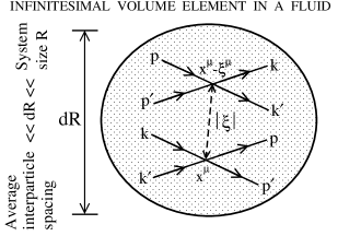
Figure 8.1: Collisions $kk^{\prime}\to pp^{\prime}$ and $pp^{\prime}\to kk^{\prime}$ occurring at points $x^{\mu}$ and $x^{\mu}-\xi^{\mu}$ within an infinitesimal fluid element of size $dR$, around $x^{\mu}$, containing a large number of particles represented by dots.

In general, for all collision types ($2\leftrightarrow 2,~{}2\leftrightarrow 3,\ldots$), the momentum dependence of the coefficients $A^{\mu}$ and $B^{\mu\nu}$ can be made explicit by expressing them in terms of the available tensors $p^{\mu}$ and the metric $g^{\mu\nu}\equiv{\rm diag}(1,-1,-1,-1)$ as $A^{\mu}=a(x)p^{\mu}$ and $B^{\mu\nu}=b_{1}(x)g^{\mu\nu}+b_{2}(x)p^{\mu}p^{\nu}$, in the spirit of Grad’s 14-moment approximation. Equation (8.1) forms the basis of our derivation of the second-order dissipative hydrodynamics.

8.3 Hydrodynamic equations

As mentioned in Chapter 2, we can express the conserved particle current and the energy-momentum tensor as [deGroot]

$$N^{\mu}=\int dp\ p^{\mu}f,\quad T^{\mu\nu}=\int dp\ p^{\mu}p^{\nu}f.$$ (8.4)

The standard tensor decomposition of the above quantities results in

$$N^{\mu} = nu^{\mu}+n^{\mu},$$

$$T^{\mu\nu} = \epsilon u^{\mu}u^{\nu}-(P+\Pi)\Delta^{\mu\nu}+\pi^{\mu\nu},$$ (8.5)

where $P,n,\epsilon$ are respectively pressure, number density, energy density, and $\Delta^{\mu\nu}=g^{\mu\nu}-u^{\mu}u^{\nu}$ is the projection operator on the three-space orthogonal to the hydrodynamic four-velocity $u^{\mu}$ defined in the Landau frame: $T^{\mu\nu}u_{\nu}=\epsilon u^{\mu}$. For small departures from equilibrium, $f(x,p)$ can be written as $f=f_{0}+\delta f$. The equilibrium distribution function is defined as $f_{0}=[\exp(\beta u\cdot p-\alpha)+r]^{-1}$ where the inverse temperature $\beta=1/T$ and $\alpha=\beta\mu$ ($\mu$ being the chemical potential) are defined by the equilibrium matching conditions $n\equiv n_{0}$ and $\epsilon\equiv\epsilon_{0}$. The scalar product is defined as $u.p\equiv u_{\mu}p^{\mu}$. The dissipative quantities, viz., the bulk viscous pressure, the particle diffusion current and the shear stress tensor are

$$\Pi = -\frac{\Delta_{\alpha\beta}}{3}\int dp\ p^{\alpha}p^{\beta}\delta f,$$

$$n^{\mu} = \Delta^{\mu\nu}\int dp\ p_{\nu}\delta f,$$

$$\pi^{\mu\nu} = \Delta^{\mu\nu}_{\alpha\beta}\int dp\ p^{\alpha}p^{\beta}\delta f.$$ (8.6)

Here $\Delta^{\mu\nu}_{\alpha\beta}=[\Delta^{\mu}_{\alpha}\Delta^{\nu}_{\beta}+\Delta^{\mu}_{\beta}\Delta^{\nu}_{\alpha}-(2/3)\Delta^{\mu\nu}\Delta_{\alpha\beta}]/2$ is the traceless symmetric projection operator. Conservation of current, $\partial_{\mu}N^{\mu}=0$ and energy-momentum tensor, $\partial_{\mu}T^{\mu\nu}=0$, yield the fundamental evolution equations for $n$, $\epsilon$ and $u^{\mu}$

$$Dn+n\partial_{\mu}u^{\mu}+\partial_{\mu}n^{\mu} = 0,$$

$$D\epsilon+(\epsilon+P+\Pi)\partial_{\mu}u^{\mu}-\pi^{\mu\nu}\nabla_{(\mu}u_{\nu)} = 0,$$

$$(\epsilon+P+\Pi)Du^{\alpha}-\nabla^{\alpha}(P+\Pi)+\Delta^{\alpha}_{\nu}\partial_{\mu}\pi^{\mu\nu} = 0.$$ (8.7)

We use the standard notation $A^{(\alpha}B^{\beta)}=(A^{\alpha}B^{\beta}+A^{\beta}B^{\alpha})/2$, $D=u^{\mu}\partial_{\mu}$, and $\nabla^{\alpha}=\Delta^{\mu\alpha}\partial_{\mu}$. For later use we introduce $X^{\langle\mu\rangle}=\Delta^{\mu}_{\nu}X^{\nu}$ and $X^{\langle\mu\nu\rangle}=\Delta^{\mu\nu}_{\alpha\beta}X^{\alpha\beta}$.

Conservation of current and energy-momentum implies vanishing zeroth and first moments of the collision term $C_{m}[f]$ in Eq. (8.1), i.e., $\int dp\ C_{m}[f]=0=\int dp\ p^{\mu}C_{m}[f]$. Moreover, the arbitrariness in $\xi^{\mu}$ requires that these conditions be satisfied at each order in $\xi^{\mu}$. Retaining terms up to second order in derivatives leads to three constraint equations for the coefficients ($a,b_{1},b_{2}$), namely $\partial_{\mu}a=0$,

$$\partial^{2}\left(b_{1}\langle 1\rangle_{0}\right)+\partial_{\mu}\partial_{\nu}\left(b_{2}\langle p^{\mu}p^{\nu}\rangle_{0}\right) = 0,$$

$$u_{\alpha}\partial_{\mu}\partial_{\nu}\left(b_{2}\langle p^{\mu}p^{\nu}p^{\alpha}\rangle_{0}\right)+u_{\alpha}\partial^{2}\left(b_{1}nu^{\alpha}\right) = 0,$$ (8.8)

where we define $\langle\cdots\rangle_{0}=\int dp(\cdots)f_{0}$. It is straightforward to show using Eq. (8.3) that the validity of the second law of thermodynamics, $\partial_{\mu}s^{\mu}\geq 0$, enforces a further constraint $|a|<1$, on the collision term $C_{m}[f]$.

In order to obtain the evolution equations for the dissipative quantities, we follow the approach as described by Denicol-Koide-Rischke (DKR) in Ref. [Denicol:2010xn]. This approach employs directly the definitions of the dissipative currents in contrast to the IS derivation which uses the second moment of the Boltzmann equation. The comoving derivatives of the dissipative quantities can be written from their definitions, Eq. (8.3), as

$$\dot{\Pi} = -\frac{\Delta_{\alpha\beta}}{3}\int dp\ p^{\alpha}p^{\beta}\delta\dot{f},$$

$$\dot{n}^{\langle\mu\rangle} = \Delta^{\mu\nu}\int dp\ p_{\nu}\delta\dot{f},$$

$$\dot{\pi}^{\langle\mu\nu\rangle} = \Delta^{\mu\nu}_{\alpha\beta}\int dp\ p^{\alpha}p^{\beta}\delta\dot{f},$$ (8.9)

where, $\dot{X}=DX$. Comoving derivative of the nonequilibrium part of the distribution function, $\delta\dot{f}$, can be obtained by writing the Boltzmann equation (8.1) in the form,

$$\delta\dot{f}=-\dot{f}_{0}-\frac{1}{u.p}p^{\mu}\nabla_{\mu}f+\frac{1}{u.p}C_{m}[f].$$ (8.10)

We note that the collision term in the Boltzmann equation, Eq. (8.2), is not written in the relaxation-time approximation, thus making it difficult to solve for the nonequilibrium distribution function using Chapman-Enskog like expansion. Therefore to proceed further, we take recourse to Grad’s 14-moment approximation [Grad] for the single-particle distribution in orthogonal basis [Denicol:2010xn], Eq. (3.8),

$$f=f_{0}+f_{0}\tilde{f}_{0}\left(\lambda_{\Pi}\Pi+\lambda_{n}n_{\alpha}p^{\alpha}+\lambda_{\pi}\pi_{\alpha\beta}p^{\alpha}p^{\beta}\right).$$ (8.11)

The coefficients ($\lambda_{\Pi},\lambda_{n},\lambda_{\pi}$) are functions of ($n,\epsilon,\beta,\alpha$). Using Eqs. (8.3)-(8.11) and introducing first-order shear tensor $\sigma_{\mu\nu}=\nabla_{\langle\mu}u_{\nu\rangle}$, vorticity $\omega_{\mu\nu}=(\nabla_{\mu}u_{\nu}-\nabla_{\nu}u_{\mu})/2$ and expansion scalar $\theta=\partial\cdot u$, we finally obtain the following evolution equations for the dissipative fluxes defined in Eq. (8.3):

$$\dot{\Pi}= -\frac{\Pi}{\tau_{\Pi}^{\prime}}-\beta_{\Pi}^{\prime}\theta-\tau_{\Pi n}^{\prime}n\cdot\dot{u}-l_{\Pi n}^{\prime}\partial\cdot n-\delta_{\Pi\Pi}^{\prime}\Pi\theta-\lambda_{\Pi n}^{\prime}n\cdot\nabla\alpha+\lambda_{\Pi\pi}^{\prime}\pi_{\mu\nu}\sigma^{\mu\nu}$$

$$+\Lambda_{\Pi\dot{u}}\dot{u}\cdot\dot{u}+\Lambda_{\Pi\omega}\omega_{\mu\nu}\omega^{\nu\mu}+(8\ {\rm terms}),$$ (8.12)

$$\dot{n}^{\langle\mu\rangle}= -\frac{n^{\mu}}{\tau_{n}^{\prime}}+\beta_{n}^{\prime}\nabla^{\mu}\alpha-\lambda_{n\omega}^{\prime}n_{\nu}\omega^{\nu\mu}-\delta_{nn}^{\prime}n^{\mu}\theta-l_{n\Pi}^{\prime}\nabla^{\mu}\Pi+l_{n\pi}^{\prime}\Delta^{\mu\nu}\partial_{\gamma}\pi^{\gamma}_{\nu}+\tau_{n\Pi}^{\prime}\Pi\dot{u}^{\mu}$$

$$-\tau_{n\pi}^{\prime}\pi^{\mu\nu}\dot{u}_{\nu}-\lambda_{n\pi}^{\prime}n_{\nu}\pi^{\mu\nu}+\lambda_{n\Pi}^{\prime}\Pi n^{\mu}+\Lambda_{n\dot{u}}\omega^{\mu\nu}\dot{u}_{\nu}+\Lambda_{n\omega}\Delta^{\mu}_{\nu}\partial_{\gamma}\omega^{\gamma\nu}+(9\ {\rm terms}),$$ (8.13)

$$\dot{\pi}^{\langle\mu\nu\rangle}= -\frac{\pi^{\mu\nu}}{\tau_{\pi}^{\prime}}+2\beta_{\pi}^{\prime}\sigma^{\mu\nu}\!-\tau_{\pi n}^{\prime}n^{\langle\mu}\dot{u}^{\nu\rangle}\!+l_{\pi n}^{\prime}\nabla^{\langle\mu}n^{\nu\rangle}\!+2\lambda_{\pi\pi}^{\prime}\pi_{\rho}^{\langle\mu}\omega^{\nu\rangle\rho}\!+\lambda_{\pi n}^{\prime}n^{\langle\mu}\nabla^{\nu\rangle}\alpha-\tau_{\pi\pi}^{\prime}\pi_{\rho}^{\langle\mu}\sigma^{\nu\rangle\rho}$$

$$-\delta_{\pi\pi}^{\prime}\pi^{\mu\nu}\theta+\Lambda_{\pi\dot{u}}\dot{u}^{\langle\mu}\dot{u}^{\nu\rangle}+\Lambda_{\pi\omega}\omega_{\rho}^{\langle\mu}\omega^{\nu\rangle\rho}+\chi_{1}\dot{b}_{2}\pi^{\mu\nu}+\chi_{2}\dot{u}^{\langle\mu}\nabla^{\nu\rangle}b_{2}+\chi_{3}\nabla^{\langle\mu}\nabla^{\nu\rangle}b_{2}.$$ (8.14)

The “8 terms” (“9 terms”) involve second-order, linear scalar (vector) combinations of derivatives of $b_{1},b_{2}$. All the terms in the above equations are inequivalent, i.e., none can be expressed as a combination of others via equations of motion [Bhattacharyya:2012ex]. All the coefficients in Eqs. (8.12)-(8.14) are obtained as functions of hydrodynamic variables. For example, some of the transport coefficients related to shear are

$$\tau_{\pi}^{\prime}=\; \beta_{\dot{\pi}}\tau_{\pi},\quad\beta_{\pi}^{\prime}=\tilde{a}\beta_{\pi}/\beta_{\dot{\pi}},\quad\beta_{\dot{\pi}}=\tilde{a}+\frac{b_{2}}{3\eta\tilde{a}}\left[\langle(u.p)^{3}\rangle_{0}-m^{2}n\right],$$

$$\beta_{\pi}=\; \frac{4}{5}P+\frac{1}{15}(\epsilon-3P)-\frac{m^{4}}{15}\left<(u.p)^{-2}\right>_{0},$$ (8.15)

where ${\tilde{a}}=(1-a)$. The rest of the coefficients can be readily calculated by performing the integrations in Eq. (8.3), in a way similar to that demonstrated in Appendix B.

Retaining only the first-order terms in Eqs. (8.12)-(8.14), and using DKR values of bulk viscosity $\zeta$, particle diffusion $\kappa$, and shear viscosity $\eta$, we get the modified first-order equations for bulk pressure $\Pi=-\tau_{\Pi}^{\prime}\beta_{\Pi}^{\prime}\theta=-\tilde{a}\zeta\theta$, heat current $n^{\mu}=\beta_{n}^{\prime}\tau_{n}^{\prime}\nabla^{\mu}\alpha$ and shear stress tensor $\pi^{\mu\nu}=2\tau_{\pi}^{\prime}\beta_{\pi}^{\prime}\sigma^{\mu\nu}=2\tilde{a}\tau_{\pi}\beta_{\pi}\sigma^{\mu\nu}=2\eta{\tilde{a}}\sigma^{\mu\nu}$. Thus the nonlocal collision term modifies even the first-order dissipative equations. This constitutes one of the main results in the present study.

If $a,\ b_{1}$ and $b_{2}$ are all set to zero, Eqs. (8.12)-(8.14) reduce to those obtained by DKR [Denicol:2010xn] with the same coefficients. Otherwise coefficients of all the terms occurring in the DKR equations get modified. Furthermore, our derivation results in new terms, for instance those with coefficients $\Lambda_{k\dot{u}}$, $\Lambda_{k\omega}$, ($k=\Pi,n,\pi$), which are absent in [Denicol:2010xn] as well as in the standard Israel-Stewart approach [Israel:1979wp]. Hence these terms have also been missed so far in the numerical studies of heavy-ion collisions in the hydrodynamic framework [Romatschke:2007mq, Song:2007ux, Luzum:2010ag]. Indeed Eqs. (8.12)-(8.14) contain all possible second-order terms allowed by symmetry considerations [Bhattacharyya:2012ex]. This is a consequence of the nonlocality of the collision term $C_{m}[f]$. However, we note that a generalization of the 14-moment approximation is also able to generate all these terms as shown recently in Ref. [Denicol:2012cn].

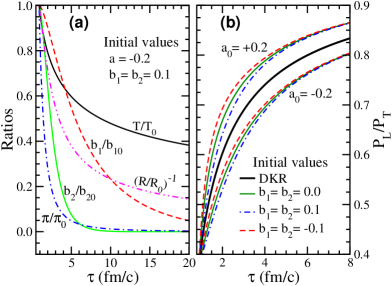
Figure 8.2: Time evolution of (a) temperature, shear pressure, inverse Reynolds number and parameters ($b_{1},\ b_{2}$) normalized to their initial values, and (b) anisotropy parameter $P_{L}/P_{T}$. Initial values are $\tau_{0}=0.9$ fm/c, $T_{0}=360$ MeV, $\eta/s=0.16$, $\pi_{0}=4\eta/(3\tau_{0})$. Units of $b_{2}$ are GeV^-2. The curve labelled DKR is obtained by setting $a=b_{1}=b_{2}=0$ in Eqs. (8.16) and (8.17).

8.4 Numerical results

To demonstrate the numerical significance of the new dissipative equations derived here, we consider evolution of a massless Boltzmann gas, with equation of state $\epsilon=3P$, at vanishing net baryon number density in the Bjorken model [Bjorken:1982qr]. The new terms, namely $\dot{u}\cdot\dot{u}$, $\omega_{\mu\nu}\omega^{\nu\mu}$, $\omega^{\mu\nu}\dot{u}_{\nu}$, $\Delta^{\mu}_{\nu}\partial_{\gamma}\omega^{\gamma\nu}$, $\dot{u}^{\langle\mu}\dot{u}^{\nu\rangle}$ and $\omega_{\rho}^{\langle\mu}\omega^{\nu\rangle\rho}$ containing acceleration and vorticity do not contribute in this case. However, they are expected to play an important role in the full 3D viscous hydrodynamics.

In terms of the coordinates ($\tau,x,y,\eta_{s}$) where $\tau=\sqrt{t^{2}-z^{2}}$ and $\eta_{s}=\tanh^{-1}(z/t)$, the initial four-velocity becomes $u^{\mu}=(1,0,0,0)$. In this scenario $\Pi=0=n^{\mu}$ and the equation for $\Phi\equiv-\tau^{2}\pi^{\eta_{s}\eta_{s}}$ reduces to (see Appendix A for details)

$$\frac{\Phi}{\tau_{\pi}}+\beta_{\dot{\pi}}\frac{d\Phi}{d\tau}=\beta_{\pi}\frac{4}{3\tau}-\lambda\frac{\Phi}{\tau}-\psi\Phi\frac{db_{2}}{d\tau},$$ (8.16)

where the coefficients are

$$\beta_{\dot{\pi}}=\tilde{a}+\frac{b_{2}(\epsilon+P)}{\tilde{a}\beta\eta},\quad\beta_{\pi}=\frac{4}{5}\tilde{a}P,\quad\psi=\frac{9(\epsilon+P)}{5\tilde{a}\beta\eta},\quad\lambda=\frac{38}{21}\tilde{a}-\!\left(\!\frac{b_{1}\beta}{5}-\frac{8b_{2}}{7\beta}\!\right)\!\frac{\epsilon+P}{\tilde{a}\eta}.$$ (8.17)

For comparison we quote the IS results [Israel:1979wp]: $\beta_{\pi}=2P/3,~{}\lambda=2$. The coupled differential equations (8.3), (8.3) and (8.16) are solved simultaneously for a variety of initial conditions: temperature $T=360$ or 500 MeV corresponding to typical RHIC and LHC energies, and shear pressure $\Phi=0$ or $\Phi=\Phi_{\rm NS}=4\eta/(3\tau_{0})$ corresponding to isotropic and anisotropic pressure configurations. Since the nonlocal effects embodied in the Taylor expansion (8.1) are not large, the initial $a,~{}b_{1},~{}b_{2}$ are so constrained that the corrections to first-order and second-order terms remain small; recall also the additional constraints $|a|<1$ and Eq. (8.3).

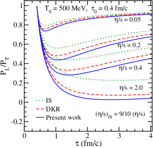
Figure 8.3: Time evolution of $P_{L}/P_{T}$ in IS [Israel:1979wp], DKR ($a=b_{1}=b_{2}=0$), and the present work, for isotropic initial pressure configuration $(\Phi_{0}=0)$. The scaling $(\eta/s)_{\rm IS}=9/10(\eta/s)$ ensures that all the results are compared at the same cross section [Denicol:2010xn].

Figure 8.2 (a) illustrates the evolution of these quantities for a choice of initial conditions. $T$ decreases monotonically to the crossover temperature $~{}170$ MeV at time $\tau\simeq 10$ fm/c, which is consistent with the expected lifetime of quark-gluon plasma. Parameter $a$ is constant whereas $b_{1}$ and $b_{2}$ vary smoothly and tend to zero at large times indicating reduced but still significant presence of nonlocal effects in the collision term at late times. This is also evident in Fig. 8.2 (b) where the pressure anisotropy $P_{L}/P_{T}=(P-\Phi)/(P+\Phi/2)$ shows marked deviation from IS, controlled mainly by $a$. At late times $P_{L}/P_{T}$ is largely unaffected by the choice of initial values of $b_{1},~{}b_{2}$. Although the shear pressure $\Phi$ vanishes rapidly indicating approach to ideal fluid dynamics, the $P_{L}/P_{T}$ is far from unity. Faster isotropization for initial $a>0$ may be attributed to a smaller effective shear viscosity $(1-a)\eta$ in the modified NS equation, and conversely. Figure 8.2 (b) also indicates the convergence of the Taylor expansion that led to Eq. (8.1).

Figure 8.3 shows the evolution of $P_{L}/P_{T}$ for isotropic initial pressure configuration, at various $\eta/s$ for the LHC energy regime. Compared to IS, DKR leads to larger pressure anisotropy. Further, with small initial corrections ($10$% to first-order and $\simeq 20$% to the second-order terms) due to $a,\ b_{1},\ b_{2}$, the nonlocal hydrodynamics (solid lines) exhibits appreciable deviation from the (local) DKR theory. The above results clearly demonstrate the importance of the nonlocal effects, which should be incorporated in transport calculations as well. Comparison of nonlocal hydrodynamics to nonlocal transport would be illuminating.

In a realistic 2+1 or 3+1 D calculation, one has to choose the thermalization time and the freeze-out temperature together with suitable initial conditions for hydrodynamic velocity, energy density, shear pressure as well as for the nonlocal coefficients $a,~{}b_{1},~{}b_{2}$ to fit $dN/d\eta$ and $p_{T}$ spectra of hadrons, and then predict, for example, the anisotropic flow $v_{n}$ for a given $\eta/s$. Nonlocal effects (especially via $a$) will affect the extraction of $\eta/s$ from fits to the measured $v_{n}$. It may also be noted that although (local) viscous hydrodynamics explains the gross features of $\pi^{-}$ and $K^{-}$ spectra for the (0-5)% most central Pb-Pb collisions at $\sqrt{s_{NN}}=2.76$ TeV, it strongly disagrees with the measured $\bar{p}$ spectrum [Floris:2011ru]. Further the constituent quark number scaling violation has been observed in the $v_{2}$ and $v_{3}$ data for $\bar{p}$, at this LHC energy [Krzewicki:2011ee]. The above discrepancies may be attributed partly to the nonlocal effects which can have different implications for two- and three-particle correlations and thus affect the meson and baryon spectra differently.

8.5 Summary and conclusions

To summarize, we have presented a new derivation of the relativistic dissipative hydrodynamic equations by introducing a nonlocal generalization of the collision term in the Boltzmann equation. The first-order and second-order equations are modified: new terms occur and coefficients of others are altered. While it is well known that the derivation based on the generalized second law of thermodynamics misses some terms in the second-order equations, we have shown that the standard derivation based on kinetic theory and 14-moment approximation also misses other terms. The method presented in this chapter is able to generate all possible terms to a given order that are allowed by symmetry. It can also be extended to derive higher order fluid dynamic equations. Within one-dimensional scaling expansion, we find that nonlocality of the collision term has a rather strong influence on the evolution of the viscous medium via hydrodynamic equations.

Chapter 9 Summary and future outlook

This thesis presents our work on the theoretical formulation of relativistic dissipative fluid dynamics from various approaches within the framework of relativistic kinetic theory. Several longstanding problems in the formulation as well as in the application of relativistic hydrodynamics relevant to heavy-ion collisions have been addressed here. The evolution equations for the dissipative quantities along with the second-order transport coefficients have been derived using the second law of thermodynamics within a single theoretical framework. In particular, the problem pertaining to the relaxation time for the evolution of bulk viscous pressure has been solved here. Subsequently, using the same method for two different forms of non-equilibrium single-particle distribution functions, viscous evolution equations have been derived and applied to study the particle production and transverse momentum spectra of hadrons and thermal dileptons.

An alternate formulation of second-order dissipative hydrodynamics has been presented in which iterative solution of the Boltzmann equation for non-equilibrium distribution function is employed instead of the 14-moment ansatz most commonly used in the literature. The evolution equations for the dissipative quantities have been obtained directly from their definitions rather than an arbitrary moment of Boltzmann equation in the traditional Israel-Stewart formulation. Using the iterative solution of Boltzmann equation, the form of second-order viscous correction to the distribution function has been derived. The effects of these corrections on particle spectra and HBT radii are compared to those due to 14-moment ansatz. This method has been further extended to obtain third-order evolution equation for shear stress tensor.

Finally, the collision term in the Boltzmann equation corresponding to $2\to 2$ elastic collisions has been modified to include the gradients of the distribution function. This non-local collision term has then been used to derive second-order evolution equations for the dissipative quantities. The numerical significance of these new formulations has been demonstrated within the framework of one-dimensional boost-invariant Bjorken expansion of the matter formed in relativistic heavy-ion collisions.

Further development of the theory of relativistic dissipative fluid dynamics requires to consider the following aspects in the future:

• More robust relaxation-time approximation: The relaxation-time approximation for the collision term significantly reduces the complexity of solving the Boltzmann equation iteratively in contrast to the situation in which the collision term captures the microscopic interaction between the constituent particles. The relaxation time $\tau_{R}$ may be either assumed to be independent of momenta or parametrized as a simple power law to reflect the momentum dependence [Dusling:2009df]. However this parametrization, commonly known as the quadratic ansatz, violates the fundamental current and energy-momentum conservation as well as the matching conditions [Jaiswal:2013vta]. To remove these inconsistencies, the momentum dependence of the relaxation time can be incorporated in a parametric form such that the conservation equations as well as the matching conditions are not violated. Further, causal dissipative relativistic fluid dynamic equations can be derived by taking into account the momentum dependence of the relaxation time via the nonequilibrium distribution function. The momentum dependence of the relaxation time may have important bearing on the extraction of $\eta/s$ of the QGP from the hydrodynamic analysis of the flow harmonics $v_{n}(p_{T})$.

• Fluid dynamics in presence of external forces: The derivation of relativistic dissipative fluid dynamics from kinetic theory proceeds by assuming Boltzmann equation in the absence of external force fields. However, experiments suggests that strong electromagnetic fields are produced in relativistic heavy-ion collisions which may have important implications on the phenomenology of QGP [Kharzeev:2007jp]. Moreover, the mean field effects due to strong interactions are non negligible and may affect the dynamics of evolution. Hence it is important to formulate fluid dynamic equations in the presence of external forces by considering the field term in the Boltzmann equation. For example, the derivation of hydrodynamic equation by employing the electromagnetic Lorentz force as the field term in the Boltzmann equation may change the effective $\eta/s$. The effects due to strong interactions can also be incorporated as a mean field term in the Boltzmann equation and then derive relativistic fluid dynamic equations.

• Complete third-order dissipative fluid dynamics: In order to improve the second-order Israel-Stewart hydrodynamics beyond its present scope, third-order evolution equations for the shear stress tensor was derived [El:2009vj, Jaiswal:2013vta, Jaiswal:2014raa]. However, these formulations are incomplete in the sense that they do not take into account the other dissipative effects such as bulk viscosity and charge diffusion current and are restricted to massless Boltzmann particles. A complete theory of relativistic third-order dissipative hydrodynamics from Boltzmann equation can be formulated. This involves extending the work done in Ref. [Jaiswal:2013vta, Jaiswal:2014raa] to a more general system, i.e. for Fermi, Bose and Boltzmann particles, and deriving evolution equations for shear stress tensor as well as bulk viscous pressure and charge diffusion current.

• General relativistic dissipative fluid dynamics: Although the Boltzmann equation can be written for a general background spacetime, in the derivation of second-order relativistic dissipative fluid dynamic equations from kinetic theory the metric is assumed to be Minkowskian [Israel:1979wp]. The resultant dissipative equations are therefore valid only in flat spacetime and are not applicable to cosmology and astrophysics. It is thus of interest to formulate hydrodynamics from kinetic theory in a metric independent manner and extend the validity of dissipative equations to a general background spacetime. Without assuming a specific form of the metric tensor, the nonequilibrium distribution function obtained after iteratively solving the general relativistic Boltzmann equation in relaxation time approximation can be used to formulate a general relativistic theory of second-order dissipative hydrodynamics. The resultant second-order coefficients can then be compared with those obtained from the strongly coupled ${\cal N}=4$ supersymmetric Yang-Mills theory [Baier:2007ix].

In conclusion, the theoretical formulation of relativistic dissipative fluid dynamics is experiencing a rapid development, with contributions from several different groups. Some major progress that we have made in the formulation of relativistic dissipative fluid dynamics, within the framework of kinetic theory, has been covered in this thesis. The work developed in this thesis has several applications to heavy-ion collisions, with implications on the evolution of the strongly interacting fluid-like matter created at RHIC and LHC. However, as outlined above, there still remains numerous interesting aspects in the formulation of relativistic dissipative fluid dynamics that need further investigation.

Appendix A Coordinates and Transformations

The three spatial coordinates and time form a four dimensional coordinate system $x^{\mu}=(t,x,y,z)$, called Cartesian coordinates. Throughout this thesis, we use the metric tensor $g_{\mu\nu}=g^{\mu\nu}=\mathrm{diag}(1,-1,-1,-1)$, such that four vectors ($x^{\mu}$, for example) transform as follows:

$$x^{\mu}=(t,x,y,z),\qquad x_{\mu}=g_{\mu\nu}x^{\nu}=(t,-x,-y,-z).$$ (A.1)

One generally sets the $z$-axis parallel to the beam direction, and correspondingly calls the $(x,y)$ plane the transverse plan (with x pointing in the direction of the impact parameter). Within the forward light-cone $|z|<t$, $\eta-\tau$ coordinates $x^{\mu}=(\tau,x,y,\eta)$ (with $\tau=\sqrt{t^{2}-z^{2}}$ and $\eta=\frac{1}{2}\ln\frac{t+z}{t-z}$) prove more useful in high energy particle and nuclear physics. The metric in this coordinate system reads $g^{\mu\nu}=\mathrm{diag}(1,-1,-1,-1/\tau^{2})$, $g_{\mu\nu}=\mathrm{diag}(1,-1,-1,-\tau^{2})$.

Here we list the transformation between Cartesian and $\eta-\tau$ coordinates:

$$\!\!\!\!\!x^{\mu}=(t,x,y,z) \!\!\!\!\!x^{\mu}=(\tau,x,y,\eta)$$

$$\!\!\!\!\!t=\tau\cosh\eta\ \ \ \!\!\!\!\!\tau=\sqrt{t^{2}-z^{2}}$$

$$\!\!\!\!\!z=\tau\sinh\eta\ \ \ \!\!\!\!\!\eta=\arctan(z/t)$$

A.1 Bjorken Flow

Bjorken’s notion of “boost invariance” is the statement that at longitudinal distance $z$ away from the point of collision and time $t$ after the collision, the matter should be moving with a velocity $v^{z}=z/t$. We neglect transverse dynamics $(v^{x}=v^{y}=0)$ and introduce Milne coordinates proper time $\tau=\sqrt{t^{2}-z^{2}}$ and spacetime rapidity $\eta=\mathrm{tanh}^{-1}(z/t)$. Hence, $t=\tau~{}\mathrm{cosh}~{}\eta$ and $z=\tau~{}\mathrm{sinh}~{}\eta$. Boost invariance for hydrodynamics simply translates into

$$u^{t}=\frac{t}{\tau}\quad;\quad u^{z}=\frac{z}{\tau}\quad;\quad u^{\eta}=-u^{t}\frac{\mathrm{sinh}~{}\eta}{\tau}+u^{z}\frac{\mathrm{cosh}~{}\eta}{\tau}=0$$ (A.2)

Hence, $u^{\mu}=(1,0,0,0)$ and as a consequence $\epsilon$, $P$, $u^{\mu}$ and $\pi^{\mu\nu}$ are all independent of $\eta$ and therefore remains unchanged when performing a Lorentz-boost. Even though in this highly simplified model the hydrodynamic degrees of freedom now only depend on proper time $\tau$, the system dynamics is not entirely trivial. The reason for this is that in Milne coordinates, the metric is given by $g_{\mu\nu}=$diag$(1,-1,-1,-\tau^{2})$ and hence is no longer co-ordinate invariant. The Christoffel symbols are non-zero and are given by

$$\Gamma^{\eta}_{\eta\tau}=\Gamma^{\eta}_{\tau\eta}=\frac{1}{\tau}\quad;\quad\Gamma^{\tau}_{\eta\eta}=\tau$$ (A.3)

Since the metric is non-trivial, we need to replace our normal derivatives with covariant derivatives. The rule for covariant differentiation of a scalar is trivial. If covariant differentiation is denoted by $d_{\mu}$ and $A$ is some scalar, then we have

$$d_{\mu}A=\partial_{\mu}A.$$ (A.4)

The rule for covariant differentiation of a vector $A^{\alpha}$ and $A_{\alpha}$ is

$$d_{\mu}A^{\alpha}=\partial_{\mu}A^{\alpha}+\Gamma^{\alpha}_{\mu\lambda}A^{\lambda}\quad;\quad d_{\mu}A_{\alpha}=\partial_{\mu}A_{\alpha}-\Gamma^{\lambda}_{\mu\alpha}A_{\lambda}.$$ (A.5)

For $\theta=\partial_{\mu}u^{\mu}$,

$$\theta=\nabla_{\mu}u^{\mu}=\Delta^{\rho}_{\mu}d_{\rho}u^{\mu}=(g^{\rho}_{\mu}-u^{\rho}u_{\mu})(\partial_{\rho}u^{\mu}+\Gamma^{\mu}_{\rho\lambda}u^{\lambda})=\Gamma^{\mu}_{\mu\lambda}u^{\lambda}=\Gamma^{\eta}_{\eta\tau}u^{\tau}=\frac{1}{\tau}.$$ (A.6)

Lets assume that $\pi^{\mu\nu}$ is diagonal with $\pi^{\tau\tau}=0$ and introduce $\Phi=-\tau^{2}\pi^{\eta\eta}$. For $\pi^{\mu\nu}$ to be traceless,

$$\pi^{\eta\eta}=-\Phi/\tau^{2}~{};\quad\pi^{xx}=\pi^{yy}=\Phi/2.$$ (A.7)

With these assumption, $\sigma^{\mu\nu}$ becomes

$$\sigma^{\mu\nu} =\Delta^{\mu\nu}_{\alpha\beta}\nabla^{\alpha}u^{\beta}=\Delta^{\mu\nu}_{\alpha\beta}\Delta^{\alpha\rho}d_{\rho}u^{\beta}=\Delta^{\mu\nu}_{\alpha\beta}\Delta^{\alpha\rho}(\partial_{\rho}u^{\beta}+\Gamma^{\beta}_{\rho\gamma}u^{\gamma})$$

$$=\Delta^{\mu\nu}_{\eta\eta}g^{\eta\eta}\Gamma^{\eta}_{\eta\tau}\quad\quad[\because\partial_{\rho}u^{\beta}=0~{}~{}\mathrm{and~{}only~{}u^{\tau}}\neq 0]$$

$$=\frac{1}{\tau}[g^{\mu}_{\eta}g^{\nu\eta}-\frac{1}{3}(g^{\mu\nu}-u^{\mu}u^{\nu})].$$ (A.8)

Therefore

$$\sigma^{\eta\eta}=\frac{1}{\tau}[g^{\eta}_{\eta}g^{\eta\eta}-\frac{1}{3}(g^{\eta\eta}-u^{\eta}u^{\eta})]=\frac{1}{\tau}[g^{\eta\eta}-\frac{1}{3}g^{\eta\eta}]=\frac{2}{3\tau}g^{\eta\eta}=-\frac{2}{3\tau^{3}}.$$ (A.9)

Next we calculate the form of the second-order terms in Bjorken case,

$$\dot{\pi}^{<\eta\eta>} =\Delta^{\eta\eta}_{\alpha\beta}u^{\mu}d_{\mu}\pi^{\alpha\beta}=[g^{\eta}_{\alpha}g^{\eta}_{\beta}-\frac{1}{3}g^{\eta\eta}(g_{\alpha\beta}-u_{\alpha}u_{\beta})]u^{\mu}d_{\mu}\pi^{\alpha\beta}=g^{\eta}_{\alpha}g^{\eta}_{\beta}u^{\mu}d_{\mu}\pi^{\alpha\beta}$$

$$=g^{\eta}_{\alpha}g^{\eta}_{\beta}u^{\mu}(\partial_{\mu}\pi^{\alpha\beta}+2\Gamma^{\alpha}_{\lambda\mu}\pi^{\lambda\beta})=\partial_{\tau}\pi^{\eta\eta}+2\frac{\pi^{\eta\eta}}{\tau}=-\frac{1}{\tau^{2}}\frac{\partial}{\partial\tau}(-\tau^{2}\pi^{\eta\eta})=-\frac{1}{\tau^{2}}\frac{\partial\Phi}{\partial\tau},$$ (A.10)

and

$$\pi^{<\eta}_{\gamma}\sigma^{\eta>\gamma} =\Delta^{\eta\eta}_{\alpha\beta}\pi^{\alpha}_{\gamma}\sigma^{\beta\gamma}=[g^{\eta}_{\alpha}g^{\eta}_{\beta}-\frac{1}{3}g^{\eta\eta}(g_{\alpha\beta}-u_{\alpha}u_{\beta})]\pi^{\alpha}_{\gamma}\sigma^{\beta\gamma}$$

$$=\pi^{\eta}_{\eta}\sigma^{\eta\eta}-\frac{1}{3}g^{\eta\eta}\pi_{\beta\gamma}\sigma^{\beta\gamma}=-\frac{2\Phi}{3\tau^{3}}+\frac{\Phi}{3\tau^{3}}=-\frac{\Phi}{3\tau^{3}}.$$ (A.11)

Hence,

$$-\tau_{\pi\pi}\,\pi^{<\eta}_{\gamma}\sigma^{\eta>\gamma}-\delta_{\pi\pi}\,\pi^{\eta\eta}\theta=\tau_{\pi\pi}\,\frac{\Phi}{3\tau^{3}}+\delta_{\pi\pi}\,\frac{\Phi}{\tau^{3}}=\left(\frac{1}{3}\tau_{\pi\pi}+\delta_{\pi\pi}\right)\frac{\Phi}{\tau^{3}}.$$ (A.12)

For the scalar $\pi^{\alpha\beta}\sigma_{\alpha\beta}$, we obtain.

$$\pi^{\alpha\beta}\sigma_{\alpha\beta} =\pi^{\alpha\beta}(\nabla_{\alpha}u_{\beta}-\frac{1}{3}\Delta_{\alpha\beta}\theta)=\pi^{\alpha\beta}\nabla_{\alpha}u_{\beta}=\pi^{\alpha\beta}\Delta^{\lambda}_{\alpha}d_{\lambda}u_{\beta}=\pi^{\lambda\beta}(\partial_{\lambda}u_{\beta}-\Gamma^{\alpha}_{\lambda\beta}u_{\alpha})$$

$$=-\pi^{\eta\eta}\tau=\frac{\Phi}{\tau}.$$ (A.13)

Similarly for third-order terms, we find that

$$\pi^{\langle\eta}_{\gamma}\pi^{\eta\rangle\gamma}\theta=-\frac{\Phi^{2}}{2\tau^{3}},\quad\pi^{\rho\langle\eta}\pi^{\eta\rangle\gamma}\sigma_{\rho\gamma}=-\frac{\Phi^{2}}{2\tau^{3}},$$ (A.14)

and

$$\nabla_{\gamma}\nabla^{<\eta}\pi^{\eta>\gamma} =\Delta^{\eta\eta}_{\alpha\beta}\nabla_{\gamma}\nabla^{\alpha}\pi^{\beta\gamma}=\frac{4\Phi}{3\tau^{4}},$$

$$\nabla^{<\eta}\nabla_{\gamma}\pi^{\eta>\gamma} =\Delta^{\eta\eta}_{\alpha\beta}\nabla^{\alpha}\nabla_{\gamma}\pi^{\beta\gamma}=\frac{2\Phi}{3\tau^{4}},$$

$$\nabla^{2}\pi^{<\eta\eta>} =\Delta^{\eta\eta}_{\alpha\beta}\nabla^{\gamma}\nabla_{\gamma}\pi^{\alpha\beta}=\frac{4\Phi}{3\tau^{4}}.$$ (A.15)

Appendix B Fluid dynamics from Chapman- Enskog expansion: Derivation details

B.1 General structure

The conserved particle current and energy-momentum tensor can be expressed in terms of the distribution function as

$$N^{\mu} =\int dp\ p^{\mu}f=nu^{\mu}+n^{\mu},$$

$$T^{\mu\nu} =\int dp\ p^{\mu}p^{\nu}f=\epsilon u^{\mu}u^{\nu}-(P+\Pi)\Delta^{\mu\nu}+\pi^{\mu\nu},$$ (B.1)

where $dp=gd{\bf p}/[(2\pi)^{3}\sqrt{{\bf p}^{2}+m^{2}}]$, $g$ and $m$ being the degeneracy factor and particle mass. In the tensor decompositions, $\epsilon,P,n$ are respectively energy density, pressure, net number density, and $\Delta^{\mu\nu}=g^{\mu\nu}-u^{\mu}u^{\nu}$ is the projection operator on the three-space orthogonal to the hydrodynamic four-velocity $u^{\mu}$ defined in the Landau frame: $T^{\mu\nu}u_{\nu}=\epsilon u^{\mu}$. The metric tensor is $g^{\mu\nu}\equiv\mathrm{diag}(+,-,-,-)$. The bulk viscous pressure $(\Pi)$, shear stress tensor $(\pi^{\mu\nu})$ and particle diffusion current $(n^{\mu})$ are the dissipative quantities. The net number density, energy density and pressure can be expressed as

$$n =u_{\mu}\int dp\ p^{\mu}f_{0},$$

$$\epsilon =u_{\mu}u_{\nu}\int dp\ p^{\mu}p^{\nu}f_{0},$$

$$P =-\frac{1}{3}\Delta_{\mu\nu}\int dp\ p^{\mu}p^{\nu}f_{0}.$$ (B.2)

The equilibrium distribution functions $f_{0}=\frac{1}{\mathrm{exp}(\beta\,u\cdot p-\alpha)+r}$ with $r=1,-1,0$ for Fermi, Bose, and Boltzmann particles. Here, $\beta=1/T$ is the inverse temperature and $\alpha=\mu/T$ is the ratio of chemical potential to temperature.

Current conservation, $\partial_{\mu}N^{\mu}=0$, and energy-momentum conservation, $\partial_{\mu}T^{\mu\nu}=0$ yields the fundamental evolution equations for $n$, $\epsilon$ and $u^{\mu}$

$$\dot{n}+n\theta+\partial_{\mu}n^{\mu} =0~{},$$ (B.3)

$$\dot{\epsilon}+(\epsilon+P+\Pi)\theta-\pi^{\mu\nu}\nabla_{(\mu}u_{\nu)} =0~{},$$ (B.4)

$$(\epsilon+P+\Pi)\dot{u}^{\alpha}-\nabla^{\alpha}(P+\Pi)+\Delta^{\alpha}_{\nu}\partial_{\mu}\pi^{\mu\nu} =0,$$ (B.5)

where, $\theta\equiv\partial_{\mu}u^{\mu}$, $\nabla^{\mu}\equiv\Delta^{\mu\nu}\partial_{\nu}$ and $\dot{u}^{\mu}\equiv Du^{\mu}=u^{\alpha}\partial_{\alpha}u^{\mu}$. Obtaining co-moving derivatives $\dot{n}$ and $\dot{\epsilon}$ from Eq. (B.2) and substituting in Eqs. (B.3) and (B.4), we arrive at

$$\dot{\beta}=\frac{J_{20}^{(0)}n-J_{10}^{(0)}(\epsilon+P)}{J_{20}^{(0)}J_{20}^{(0)}-J_{30}^{(0)}J_{10}^{(0)}}~{}\theta+\mathcal{O}(\delta^{2}),\quad\dot{\alpha}=\frac{J_{30}^{(0)}n-J_{20}^{(0)}(\epsilon+P)}{J_{20}^{(0)}J_{20}^{(0)}-J_{30}^{(0)}J_{10}^{(0)}}~{}\theta+\mathcal{O}(\delta^{2}),$$ (B.6)

where $\mathcal{O}(\delta^{2})$ means second-order in gradients. We define the thermodynamic functions,

$$J_{nq}^{(m)}=\frac{(-1)^{q}}{(2q+1)!!}\int dp~{}(u\!\cdot\!p)^{n-2q-m}(\Delta_{\alpha\beta}p^{\alpha}p^{\beta})^{q}f_{0}\tilde{f}_{0},$$ (B.7)

where $\tilde{f}_{0}=1-rf_{0}$. We similarly define

$$I_{nq}^{(m)}=\frac{(-1)^{q}}{(2q+1)!!}\int dp~{}(u\!\cdot\!p)^{n-2q-m}(\Delta_{\alpha\beta}p^{\alpha}p^{\beta})^{q}f_{0},$$ (B.8)

and state the relations

$$J_{nq}^{(0)}=\frac{1}{\beta}\left[-I_{n-1,q-1}^{(0)}+(n-2q)I_{n-1,q}^{(0)}\right];\quad I_{10}^{(0)}=n,\quad I_{20}^{(0)}=\epsilon,\quad I_{21}^{(0)}=-P.$$ (B.9)

Substituting the space-like derivative of pressure ($\nabla^{\alpha}P$) obtained from Eq. (B.2) in Eq. (B.5) and using Eq. (B.9), we get,

$$\nabla^{\mu}\beta=-\beta\dot{u}^{\mu}+\frac{n}{\epsilon+P}\nabla^{\mu}\alpha+\mathcal{O}(\delta^{2}),$$ (B.10)

The expressions for the dissipative quantities in terms of away from equilibrium part of the distribution functions ($\delta f$), can be written using Eq. (B.1) as

$$\Pi =-\frac{\Delta_{\alpha\beta}}{3}\int dp\,p^{\alpha}p^{\beta}\delta f,$$ (B.11)

$$n^{\mu} =\Delta^{\mu}_{\alpha}\int dp\,p^{\alpha}\delta f,$$ (B.12)

$$\pi^{\mu\nu} =\Delta^{\mu\nu}_{\alpha\beta}\int dp\,p^{\alpha}p^{\beta}\delta f,$$ (B.13)

where $\Delta^{\mu\nu}_{\alpha\beta}=[\Delta^{\mu}_{\alpha}\Delta^{\nu}_{\beta}+\Delta^{\mu}_{\beta}\Delta^{\nu}_{\alpha}-(2/3)\Delta^{\mu\nu}\Delta_{\alpha\beta}]/2$.

To obtain $\delta f$, we solve Boltzmann equation in relaxation time approximation using Chapman-Enskog (CE) expansion. In the CE expansion, the particle distribution function is expanded about its equilibrium value in powers of space-time gradients.

$$f=f_{0}+\delta f,\quad\delta f=\delta f^{(1)}+\delta f^{(2)}+\cdots,$$ (B.14)

where $\delta f^{(1)}$ is first-order in gradients, $\delta f^{(2)}$ is second-order, etc. The Boltzmann equation, $p^{\mu}\partial_{\mu}f=-(u\!\cdot\!p)\delta f/\tau_{R}$, in the form $f=f_{0}-(\tau_{R}/u\!\cdot\!p)\,p^{\mu}\partial_{\mu}f$, can be solved iteratively as

$$f_{1}=f_{0}-\frac{\tau_{R}}{u\!\cdot\!p}\,p^{\mu}\partial_{\mu}f_{0},\quad f_{2}=f_{0}-\frac{\tau_{R}}{u\!\cdot\!p}\,p^{\mu}\partial_{\mu}f_{1},~{}~{}\,\cdots$$ (B.15)

where $f_{1}=f_{0}+\delta f^{(1)}$ and $f_{2}=f_{0}+\delta f^{(1)}+\delta f^{(2)}$. To first and second-order in gradients,

$$\delta f^{(1)}=-\frac{\tau_{R}}{u\!\cdot\!p}\,p^{\mu}\partial_{\mu}f_{0},\quad\delta f^{(2)}=\frac{\tau_{R}}{u\!\cdot\!p}p^{\mu}p^{\nu}\partial_{\mu}\Big{(}\frac{\tau_{R}}{u\!\cdot\!p}\partial_{\nu}f_{0}\Big{)}.$$ (B.16)

B.2 First-order equations

The first-order dissipative equations can be obtained from Eqs. (B.11)-(B.13) using $\delta f=\delta f^{(1)}$ from Eq. (B.16)

$$\Pi =-\frac{\Delta_{\alpha\beta}}{3}\int dp\,p^{\alpha}p^{\beta}\left(-\frac{\tau_{R}}{u\!\cdot\!p}\,p^{\gamma}\partial_{\gamma}f_{0}\right),$$ (B.17)

$$n^{\mu} =\Delta^{\mu}_{\alpha}\int dp\,p^{\alpha}\left(-\frac{\tau_{R}}{u\!\cdot\!p}\,p^{\gamma}\partial_{\gamma}f_{0}\right),$$ (B.18)

$$\pi^{\mu\nu} =\Delta^{\mu\nu}_{\alpha\beta}\int dp\ p^{\alpha}p^{\beta}\left(-\frac{\tau_{R}}{u\!\cdot\!p}\,p^{\gamma}\partial_{\gamma}f_{0}\right).$$ (B.19)

Assuming the relaxation time $\tau_{R}$ to be independent of four-momenta, the integrals in Eqs. (B.17)-(B.19) reduce to (see next section for details)

$$\Pi=-\tau_{R}\beta_{\Pi}\theta,~{}~{}n^{\mu}=\tau_{R}\beta_{n}\nabla^{\mu}\alpha,~{}~{}\pi^{\mu\nu}=2\tau_{R}\beta_{\pi}\sigma^{\mu\nu},$$ (B.20)

where $\sigma^{\mu\nu}=\Delta^{\mu\nu}_{\alpha\beta}\nabla^{\alpha}u^{\beta}$. The coefficients $\beta_{\Pi},~{}\beta_{n}$ and $\beta_{\pi}$ are found to be

$$\beta_{\Pi}= ~{}\frac{1}{3}\left(1-3c_{s}^{2}\right)(\epsilon+P)-\frac{2}{9}(\epsilon-3P)-\frac{m^{4}}{9}\left<(u\!\cdot\!p)^{-2}\right>_{0},$$ (B.21)

$$\beta_{n}= ~{}-\frac{n^{2}}{\beta(\epsilon+P)}+\frac{2\left<1\right>_{0}}{3\beta}+\frac{m^{2}}{3\beta}\left<(u\!\cdot\!p)^{-2}\right>_{0},$$ (B.22)

$$\beta_{\pi}= ~{}\frac{4P}{5}+\frac{\epsilon-3P}{15}-\frac{m^{4}}{15}\left<(u\!\cdot\!p)^{-2}\right>_{0},$$ (B.23)

where $\left<\cdots\right>_{0}=\int dp(\cdots)f_{0}$, and $c_{s}^{2}=(dP/d\epsilon)_{s/n}$ is the adiabatic speed of sound squared ($s$ being the entropy density).

B.3 Second-order evolution equations

Substituting $\delta f=\delta f^{(1)}+\delta f^{(2)}$ from Eq. (B.16) in Eq. (B.13) and assuming a momentum-independent relaxation time, we obtain

$$\frac{\pi^{\mu\nu}}{\tau_{R}}=-\Delta^{\mu\nu}_{\alpha\beta}\int dp\,p^{\alpha}p^{\beta}\left[\frac{p^{\gamma}}{u\!\cdot\!p}\partial_{\gamma}f_{0}-\frac{p^{\gamma}p^{\rho}}{u\!\cdot\!p}\partial_{\gamma}\left(\frac{\tau_{R}}{u\!\cdot\!p}\partial_{\rho}f_{0}\right)\right].$$ (B.24)

The first-order term can be solved as

$$\frac{\pi^{\mu\nu}_{(1)}}{\tau_{R}} =\Delta^{\mu\nu}_{\alpha\beta}\int dp\,p^{\alpha}p^{\beta}\left(-\frac{1}{u\!\cdot\!p}\,p^{\gamma}\partial_{\gamma}f_{0}\right)$$

$$=\Delta^{\mu\nu}_{\alpha\beta}\int\frac{dp}{u\!\cdot\!p}\,p^{\alpha}p^{\beta}p^{\gamma}\left[\{(u\!\cdot\!p)\partial_{\gamma}\beta+\beta(\partial_{\gamma}u_{\lambda})p^{\lambda}-(\partial_{\gamma}\alpha)\}f_{0}\tilde{f}_{0}\right]$$

$$=\Delta^{\mu\nu}_{\alpha\beta}\left[(\partial_{\gamma}\beta)J_{(0)}^{\alpha\beta\gamma}+\beta(\partial_{\gamma}u_{\lambda})J_{(1)}^{\alpha\beta\gamma\lambda}-(\partial_{\gamma}\alpha)J_{(1)}^{\alpha\beta\gamma}\right]$$

$$=2\,\beta J^{(1)}_{42}\sigma^{\mu\nu},$$ (B.25)

where $\sigma^{\mu\nu}=\Delta^{\mu\nu}_{\alpha\beta}(\nabla_{\alpha}u_{\beta})$ and $\beta J^{(1)}_{42}$ can be reduced to $\beta_{\pi}$ after some algebra.

The second-order terms are given by

$$\frac{\pi^{\mu\nu}_{(2)}}{\tau_{R}} =\Delta^{\mu\nu}_{\alpha\beta}\int dp\,p^{\alpha}p^{\beta}~{}\frac{p^{\gamma}p^{\rho}}{u\!\cdot\!p}\partial_{\gamma}\left(\frac{\tau_{R}}{u\!\cdot\!p}\partial_{\rho}f_{0}\right)$$

$$=\Delta^{\mu\nu}_{\alpha\beta}\int dp\,p^{\alpha}p^{\beta}\Big{[}\underbrace{D\left(\frac{\tau_{R}}{u\!\cdot\!p}p^{\rho}\partial_{\rho}f_{0}\right)}_{{}(I)}+\underbrace{\frac{p^{\gamma}}{u\!\cdot\!p}\nabla_{\gamma}(\tau_{R}\dot{f}_{0})}_{{}(II)}+\underbrace{\frac{p^{\gamma}}{u\!\cdot\!p}\nabla_{\gamma}\left(\frac{\tau_{R}}{u\!\cdot\!p}p^{\rho}\nabla_{\rho}f_{0}\right)}_{{}(III)}\Big{]}.$$ (B.26)

We perform the integrals one-by-one.

$$(I) =\Delta^{\mu\nu}_{\alpha\beta}D\left(\tau_{R}\!\int\!\frac{dp}{u\!\cdot\!p}\,p^{\alpha}p^{\beta}p^{\rho}\partial_{\rho}f_{0}\right)$$

$$=-\Delta^{\mu\nu}_{\alpha\beta}D\left[\tau_{R}\!\int\!\frac{dp}{u\!\cdot\!p}\,p^{\alpha}p^{\beta}p^{\rho}\left\{(u\!\cdot\!p)\partial_{\rho}\beta+\beta(\partial_{\rho}u_{\lambda})p^{\lambda}-(\partial_{\rho}\alpha)\right\}f_{0}\tilde{f}_{0}\right]$$

$$=-\Delta^{\mu\nu}_{\alpha\beta}D\left[\tau_{R}\,\beta\,(\nabla_{\rho}u_{\lambda})J^{\alpha\beta\rho\lambda}_{(1)}\right]$$

$$=-\Delta^{\mu\nu}_{\alpha\beta}D\left[2\,\tau_{R}\,\beta\,J^{(1)}_{42}\sigma_{\alpha\beta}\right]$$

$$=-\dot{\pi}^{\langle\mu\nu\rangle},$$ (B.27)

where $A^{\langle\mu\nu\rangle}=\Delta^{\mu\nu}_{\alpha\beta}A_{\alpha\beta}$. Eqs. (B.9) and (B.10) has been used to arrive at the third step. In the last step, the first-order Eq. (B.25) has been used ($\dot{\pi}^{\langle\mu\nu\rangle}_{(1)}=\dot{\pi}^{\langle\mu\nu\rangle}+\mathcal{O}(\delta^{3})$).

Keeping in mind that $\dot{f}_{0}=-[(u\cdot p)\dot{\beta}+\beta p^{\lambda}\dot{u}_{\lambda}-\dot{\alpha}]f_{0}\tilde{f}_{0}$, we solve the second term

$$(II) =\Delta^{\mu\nu}_{\alpha\beta}\!\int\!\frac{dp}{u\!\cdot\!p}\,p^{\alpha}p^{\beta}p^{\gamma}\,\nabla_{\gamma}(\tau_{R}\dot{f}_{0})$$

$$=\Delta^{\mu\nu}_{\alpha\beta}\nabla_{\gamma}\left(\tau_{R}\!\int\!\frac{dp}{u\!\cdot\!p}\,p^{\alpha}p^{\beta}p^{\gamma}\,\dot{f}_{0}\right)+\Delta^{\mu\nu}_{\alpha\beta}(\nabla_{\gamma}u_{\rho})\tau_{R}\!\int\!\frac{dp}{(u\!\cdot\!p)^{2}}\,p^{\alpha}p^{\beta}p^{\gamma}p^{\rho}\,\dot{f}_{0}$$

$$=-2\,\tau_{R}\left[\left(J^{(0)}_{31}+J^{(1)}_{42}\right)\dot{\beta}-\left(J^{(1)}_{31}+J^{(2)}_{42}\right)\dot{\alpha}\right]\sigma^{\mu\nu}-2\nabla^{\langle\mu}\left(\dot{u}^{\nu\rangle}\tau_{R}\beta J^{(1)}_{42}\right).$$ (B.28)

Similarly, writing $\nabla_{\rho}f_{0}=-[(u\cdot p)\nabla_{\rho}\beta+\beta(\nabla_{\rho}u_{\lambda})p^{\lambda}-(\nabla_{\rho}\alpha)]f_{0}\tilde{f}_{0}$, and using Eq. (B.10) the third term becomes

$$(III)= ~{}2\nabla^{\langle\mu}\!\left(\dot{u}^{\nu\rangle}\tau_{R}\beta J^{(1)}_{42}\right)\!+2\nabla^{\langle\mu}\!\left[\left(\nabla^{\nu\rangle}\alpha\right)\tau_{R}\left(J^{(2)}_{42}\!-\frac{n}{\epsilon+P}J^{(1)}_{42}\right)\!\right]\!+4\tau_{R}\beta J^{(1)}_{42}\sigma_{\gamma}^{\langle\mu}\omega^{\nu\rangle\gamma}$$

$$-\frac{4}{3}\,\beta\tau_{R}\left(7J^{(3)}_{63}+5J^{(1)}_{42}\right)\theta\sigma^{\mu\nu}-4\beta\tau_{R}\left(2J^{(3)}_{63}+J^{(1)}_{42}\right)\sigma_{\gamma}^{\langle\mu}\sigma^{\nu\rangle\gamma}.$$ (B.29)

We observe that the last term in Eq. (B.28) and the first term in Eq. (B.29) cancels. Adding Eqs. (B.27)-(B.29), we obtain

$$\frac{\pi^{\mu\nu}_{(2)}}{\tau_{R}}= -\dot{\pi}^{\langle\mu\nu\rangle}-2\,\tau_{R}\left[\left(J^{(0)}_{31}+J^{(1)}_{42}\right)\dot{\beta}-\left(J^{(1)}_{31}+J^{(2)}_{42}\right)\dot{\alpha}\right]\sigma^{\mu\nu}+4\tau_{R}\beta J^{(1)}_{42}\sigma_{\gamma}^{\langle\mu}\omega^{\nu\rangle\gamma}$$

$$+2\nabla^{\langle\mu}\!\left[\left(\nabla^{\nu\rangle}\alpha\right)\tau_{R}\left(J^{(2)}_{42}-\frac{n}{\epsilon+P}J^{(1)}_{42}\right)\!\right]-\frac{4}{3}\,\beta\tau_{R}\left(7J^{(3)}_{63}+5J^{(1)}_{42}\right)\theta\sigma^{\mu\nu}$$

$$-4\beta\tau_{R}\left(2J^{(3)}_{63}+J^{(1)}_{42}\right)\sigma_{\gamma}^{\langle\mu}\sigma^{\nu\rangle\gamma}.$$ (B.30)

Adding Eqs. (B.25) and (B.30) and using Eq. (B.6) and (B.10), we get the final evolution equation for shear stress tensor,

$$\frac{\pi^{\mu\nu}}{\tau_{R}}= -\dot{\pi}^{\langle\mu\nu\rangle}+2\beta_{\pi}\sigma^{\mu\nu}+2\pi_{\gamma}^{\langle\mu}\omega^{\nu\rangle\gamma}-\tau_{\pi\pi}\pi_{\gamma}^{\langle\mu}\sigma^{\nu\rangle\gamma}-\delta_{\pi\pi}\pi^{\mu\nu}\theta+\lambda_{\pi\Pi}\Pi\sigma^{\mu\nu}-\tau_{\pi n}n^{\langle\mu}\dot{u}^{\nu\rangle}$$

$$+\lambda_{\pi n}n^{\langle\mu}\nabla^{\nu\rangle}\alpha+\ell_{\pi n}\nabla^{\langle\mu}n^{\nu\rangle},$$ (B.31)

where,

$$\tau_{\pi\pi}=\, 2\beta\!\left(\!2J^{(3)}_{63}+J^{(1)}_{42}\!\right)\!\!/\beta_{\pi},\quad\delta_{\pi\pi}=\frac{1}{3}\beta\!\left(\!7J^{(3)}_{63}+5J^{(1)}_{42}\!\right)\!\!/\beta_{\pi},\quad\ell_{\pi n}=2\!\left(\!J^{(2)}_{42}-\frac{n}{\epsilon+P}J^{(1)}_{42}\!\right)\!\!/\beta_{n}$$

$$\lambda_{\pi\Pi}=\, 2\bigg{[}\left(J^{(0)}_{31}+J^{(1)}_{42}\right)\frac{J_{20}^{(0)}n-J_{10}^{(0)}(\epsilon+P)}{J_{20}^{(0)}J_{20}^{(0)}-J_{30}^{(0)}J_{10}^{(0)}}-\left(J^{(1)}_{31}+J^{(2)}_{42}\right)\frac{J_{30}^{(0)}n-J_{20}^{(0)}(\epsilon+P)}{J_{20}^{(0)}J_{20}^{(0)}-J_{30}^{(0)}J_{10}^{(0)}}$$

$$\quad+\frac{1}{3}\beta\left(7J^{(3)}_{63}+5J^{(1)}_{42}\right)\bigg{]}/\beta_{\Pi}.$$ (B.32)

The coefficients $\tau_{\pi n}$ and $\lambda_{\pi n}$ contain derivatives of $\ell_{\pi n}$.

Proceeding in a similar way, the evolution equations for bulk pressure and particle diffusion current can also be obtained. For bulk pressure, we get the expression

$$\frac{\Pi}{\tau_{R}}=-\dot{\Pi}-\beta_{\Pi}\theta-\delta_{\Pi\Pi}\Pi\theta+\lambda_{\Pi\pi}\pi^{\mu\nu}\sigma_{\mu\nu}-\tau_{\Pi n}n\cdot\dot{u}-\lambda_{\Pi n}n\cdot\nabla\alpha-\ell_{\Pi n}\partial\cdot n,\\$$ (B.33)

where,

$$\delta_{\Pi\Pi}=\, \frac{5}{3}\bigg{[}\left(J^{(0)}_{31}+J^{(1)}_{42}\right)\frac{J_{20}^{(0)}n-J_{10}^{(0)}(\epsilon+P)}{J_{20}^{(0)}J_{20}^{(0)}-J_{30}^{(0)}J_{10}^{(0)}}-\left(J^{(1)}_{31}+J^{(2)}_{42}\right)\frac{J_{30}^{(0)}n-J_{20}^{(0)}(\epsilon+P)}{J_{20}^{(0)}J_{20}^{(0)}-J_{30}^{(0)}J_{10}^{(0)}}$$

$$\quad~{}+\frac{1}{3}\,\beta\left(7J^{(3)}_{63}+\frac{23}{5}J^{(1)}_{42}\right)\bigg{]}/\beta_{\Pi},$$

$$\lambda_{\Pi\pi}=\, \frac{1}{3}\,\beta\left(7J^{(3)}_{63}+J^{(1)}_{42}\right)\!/\beta_{\pi},\quad\ell_{\Pi n}=\frac{5}{3}\left(J^{(2)}_{42}-\frac{n}{\epsilon+P}J^{(1)}_{42}\right)\!/\beta_{n}.$$ (B.34)

The coefficients $\tau_{\Pi n}$ and $\lambda_{\Pi n}$ contain derivatives of $\ell_{\Pi n}$.

Finally, the second-order evolution equation for particle diffusion current can also be derived by performing a similar kind of calculation.

$$\frac{n^{\mu}}{\tau_{R}}= -\dot{n}^{\langle\mu\rangle}+\beta_{n}\nabla^{\mu}\alpha-n_{\nu}\omega^{\nu\mu}-\lambda_{nn}n^{\nu}\sigma_{\nu}^{\mu}-\delta_{nn}n^{\mu}\theta+\lambda_{n\Pi}\Pi\nabla^{\mu}\alpha-\lambda_{n\pi}\pi^{\mu\nu}\nabla_{\nu}\alpha-\tau_{n\pi}\pi_{\nu}^{\mu}\dot{u}^{\nu}$$

$$+\tau_{n\Pi}\Pi\dot{u}^{\mu}+\ell_{n\pi}\Delta^{\mu\nu}\partial_{\gamma}\pi_{\nu}^{\gamma}-\ell_{n\Pi}\nabla^{\mu}\Pi~{},$$ (B.35)

where,

$$\lambda_{nn}=\, 1\!+\!2\!\left(\!\frac{nJ^{(2)}_{42}}{\epsilon+P}-J^{(3)}_{42}\!\right)\!\!/\beta_{n},\quad\delta_{nn}=\frac{4}{3}\!+\!\frac{5}{3}\!\left(\!\frac{nJ^{(2)}_{42}}{\epsilon+P}-J^{(3)}_{42}\!\right)\!\!/\beta_{n},\quad\ell_{n\pi}=-\left(\!\beta J^{(2)}_{42}\!\right)\!\!/\beta_{\pi},$$

$$\ell_{n\Pi}=\, -\left(\!J^{(0)}_{21}\frac{J_{20}^{(0)}n-J_{10}^{(0)}(\epsilon+P)}{J_{20}^{(0)}J_{20}^{(0)}-J_{30}^{(0)}J_{10}^{(0)}}-J^{(1)}_{21}\frac{J_{30}^{(0)}n-J_{20}^{(0)}(\epsilon+P)}{J_{20}^{(0)}J_{20}^{(0)}-J_{30}^{(0)}J_{10}^{(0)}}+\frac{5}{3}\beta J^{(1)}_{42}\!\right)\!\!/\beta_{\Pi}.$$ (B.36)

The coefficients $\tau_{n\pi}$ and $\lambda_{n\pi}$ contain derivatives of $\ell_{n\pi}$ and the coefficients $\tau_{n\Pi}$ and $\lambda_{n\Pi}$ contain derivatives of $\ell_{n\Pi}$.

Appendix C Effect of second-order viscous correction to the distribution function

C.1 Constraints on the viscous correction to the distribution function

In this appendix, we show that the form of the viscous correction to the distribution function, $\delta f$, given in Eq. (6.13) satisfies the matching condition $\epsilon=\epsilon_{0}$ and the Landau frame definition $u_{\nu}T^{\mu\nu}=\epsilon u^{\mu}$, at each order in gradients [deGroot]. We also show that $\delta f$ is consistent with the definition of the shear stress tensor, Eq. (6.5).

The first- and second-order viscous corrections to the distribution function can be written separately using Eq. (6.13). The first-order correction is given by

$$\delta f_{1}=\frac{f_{0}\beta}{2\beta_{\pi}(u\!\cdot\!p)}\,p^{\alpha}p^{\beta}\pi_{\alpha\beta},$$ (C.1)

whereas the second-order correction is

$$\delta f_{2}\!= -\frac{f_{0}\beta}{\beta_{\pi}}\bigg{[}\frac{\tau_{\pi}}{u\!\cdot\!p}\,p^{\alpha}p^{\beta}\pi^{\gamma}_{\alpha}\,\omega_{\beta\gamma}-\frac{5}{14\beta_{\pi}(u\!\cdot\!p)}\,p^{\alpha}p^{\beta}\pi^{\gamma}_{\alpha}\,\pi_{\beta\gamma}$$

$$+\!\frac{\tau_{\pi}}{3(u\!\cdot\!p)}p^{\alpha}p^{\beta}\pi_{\alpha\beta}\theta-\frac{6\tau_{\pi}}{5}p^{\alpha}\dot{u}^{\beta}\pi_{\alpha\beta}+\!\frac{(u\!\cdot\!p)}{70\beta_{\pi}}\pi^{\alpha\beta}\pi_{\alpha\beta}$$

$$+\frac{\tau_{\pi}}{5}p^{\alpha}\!\left(\!\nabla^{\beta}\pi_{\alpha\beta}\!\right)\!-\frac{3\tau_{\pi}}{(u\!\cdot\!p)^{2}}\,p^{\alpha}p^{\beta}p^{\gamma}\pi_{\alpha\beta}\dot{u}_{\gamma}\!+\frac{\tau_{\pi}}{2(u\!\cdot\!p)^{2}}$$

$$\times\!p^{\alpha}p^{\beta}p^{\gamma}\!\left(\nabla_{\gamma}\pi_{\alpha\beta}\!\right)-\frac{\beta\!+\!(u\!\cdot\!p)^{-1}}{4(u\!\cdot\!p)^{2}\beta_{\pi}}\!\left(p^{\alpha}p^{\beta}\pi_{\alpha\beta}\!\right)^{\!2}\!\bigg{]}.$$ (C.2)

In the following, we show that the $\delta f_{i}$ given in Eqs. (C.1) and (C.1) satisfies the conditions

$$L_{1}[\delta f_{i}]\equiv\int dp\,(u\cdot p)^{2}\,\delta f_{i}=0,$$ (C.3)

corresponding to $\epsilon=\epsilon_{0}$, and

$$L_{2}[\delta f_{i}]\equiv\int dp\,\Delta_{\mu\alpha}u_{\beta}\,p^{\alpha}p^{\beta}\,\delta f_{i}=0,$$ (C.4)

corresponding to $u_{\nu}T^{\mu\nu}=\epsilon u^{\mu}$.

At first order, we obtain

$$L_{1}[\delta f_{1}]=\frac{\beta}{2\beta_{\pi}}\pi_{\alpha\beta}u_{\gamma}I_{(0)}^{\alpha\beta\gamma},\quad\!L_{2}[\delta f_{1}]=\frac{\beta}{2\beta_{\pi}}\pi_{\alpha\beta}\Delta_{\mu\gamma}I_{(0)}^{\alpha\beta\gamma},$$ (C.5)

where we define the integral

$$I^{\mu_{1}\mu_{2}\cdots\mu_{n}}_{(r)}\equiv\int\frac{dp}{(u\!\cdot\!p)^{r}}p^{\mu_{1}}p^{\mu_{2}}\cdots p^{\mu_{n}}f_{0}.$$ (C.6)

The above momentum integral can be decomposed into hydrodynamic tensor degrees of freedom as

$$I^{\mu_{1}\mu_{2}\cdots\mu_{n}}_{(r)}=\ I_{n0}^{(r)}u^{\mu_{1}}u^{\mu_{2}}\cdots u^{\mu_{n}}+I_{n1}^{(r)}\big{(}\Delta^{\mu_{1}\mu_{2}}u^{\mu_{3}}\cdots u^{\mu_{n}}$$

$$+\mathrm{perms}\big{)}+\cdots,$$ (C.7)

where we readily identify $I_{20}^{(0)}=\epsilon$ and $I_{21}^{(0)}=-P$. Using the above tensor decomposition for $I_{(0)}^{\alpha\beta\gamma}$ in Eq. (C.5), we obtain

$$L_{1}[\delta f_{1}]=0,\quad L_{2}[\delta f_{1}]=0.$$ (C.8)

Similarly, for second-order corrections given in Eq. (C.1), we obtain

$$L_{1}[\delta f_{2}]= \,0+\!\frac{5\beta}{14\beta_{\pi}^{2}}\pi_{\alpha\beta}\pi^{\alpha\beta}\!I_{31}^{(0)}\!+0+0-\!\frac{\beta}{70\beta_{\pi}^{2}}\pi_{\alpha\beta}\pi^{\alpha\beta}\!I_{30}^{(0)}$$

$$-\frac{\beta\tau_{\pi}}{5\beta_{\pi}}(\nabla^{\alpha}\pi_{\alpha\beta})I_{30}^{(0)}u^{\beta}+0-\frac{\beta\tau_{\pi}}{\beta_{\pi}}(\nabla_{\gamma}\pi_{\alpha\beta})I_{31}^{(0)}$$

$$\times\!u^{(\alpha}\Delta^{\beta)\gamma}+\frac{\beta}{2\beta_{\pi}^{2}}\pi_{\alpha\beta}\pi^{\alpha\beta}\!\left(\beta I_{42}^{(0)}+I_{42}^{(1)}\right).$$ (C.9)

Using the identities

$$I_{nq}^{(r)} =-\frac{1}{2q+1}I_{n-1,q-1}^{(r-1)},$$ (C.10)

$$I_{nq}^{(0)} =\frac{1}{\beta}\left[-I_{n-1,q-1}^{(0)}+(n-2q)I_{n-1,q}^{(0)}\right],$$ (C.11)

and Eq. (6.11), we obtain

$$L_{1}[\delta f_{2}]= \,-\frac{25}{14\beta_{\pi}}\pi_{\alpha\beta}\pi^{\alpha\beta}\!-\frac{3}{14\beta_{\pi}}\pi_{\alpha\beta}\pi^{\alpha\beta}\!+\frac{12}{8\beta_{\pi}}\pi_{\alpha\beta}\pi^{\alpha\beta}$$

$$-\frac{5}{2\beta_{\pi}}\pi_{\alpha\beta}\pi^{\alpha\beta}+\frac{3}{\beta_{\pi}}\pi_{\alpha\beta}\pi^{\alpha\beta}$$

$$= \,0.$$ (C.12)

A similar calculation leads to

$$L_{2}[\delta f_{2}]= \,0+0+0+\frac{6\beta\tau_{\pi}}{5\beta_{\pi}}I_{31}^{(0)}\Delta_{\mu}^{\alpha}\dot{u}^{\beta}\pi_{\alpha\beta}+0$$

$$-\frac{\beta\tau_{\pi}}{5\beta_{\pi}}I_{31}^{(0)}\Delta_{\mu}^{\alpha}\left(\!\nabla^{\beta}\pi_{\alpha\beta}\!\right)-\frac{6\beta\tau_{\pi}}{5\beta_{\pi}}I_{31}^{(0)}\Delta_{\mu}^{\alpha}\dot{u}^{\beta}\pi_{\alpha\beta}$$

$$-\frac{\beta\tau_{\pi}}{\beta_{\pi}}I_{42}^{(1)}\Delta_{\mu}^{\alpha}\left(\!\nabla^{\beta}\pi_{\alpha\beta}\!\right)+0$$

$$= \,0.$$ (C.13)

To obtain the second equality, we have used Eq. (C.10) to replace $I_{42}^{(1)}=-I_{31}^{(0)}/5$.

Next we show that the form of the viscous correction to the distribution function, $\delta f=\delta f_{1}+\delta f_{2}$ given in Eqs. (C.1) and (C.1), is consistent with the definition of the shear stress tensor given in Eq. (6.5). In other words, we show that $\pi^{\mu\nu}=L_{3}[\delta f_{1}]+L_{3}[\delta f_{2}]$, where

$$L_{3}[\delta f_{i}]\equiv\Delta^{\mu\nu}_{\alpha\beta}\int dp\,p^{\alpha}p^{\beta}\,\delta f_{i}.$$ (C.14)

At first order, we get

$$L_{3}[\delta f_{1}]=\frac{\beta}{2\beta_{\pi}}\,\Delta^{\mu\nu}_{\alpha\beta}\,\pi_{\gamma\delta}\,I_{(1)}^{\alpha\beta\gamma\delta}.$$ (C.15)

Using the tensor decomposition for $I_{(1)}^{\alpha\beta\gamma\delta}$ in the above equation, we obtain

$$L_{3}[\delta f_{1}]=\frac{\beta}{\beta_{\pi}}\,I^{(1)}_{42}\,\pi^{\mu\nu}=\pi^{\mu\nu}.$$ (C.16)

Here we have used $I^{(1)}_{42}=\beta_{\pi}/\beta$, obtained by employing the recursion relations, Eqs. (C.10) and (C.11).

Similarly, for the second-order correction $\delta f_{2}$ given in Eq. (C.1), we obtain

$$L_{3}[\delta f_{2}]= \,-2\tau_{\pi}\pi_{\gamma}^{\langle\mu}\omega^{\nu\rangle\gamma}+\frac{5}{7\beta_{\pi}}\pi_{\gamma}^{\langle\mu}\pi^{\nu\rangle\gamma}-\frac{2}{3}\tau_{\pi}\pi^{\mu\nu}\theta+0$$

$$+0+0+0+\Big{(}\frac{1}{\beta_{\pi}}\pi_{\gamma}^{\langle\mu}\pi^{\nu\rangle\gamma}+2\tau_{\pi}\pi_{\gamma}^{\langle\mu}\omega^{\nu\rangle\gamma}$$

$$+\frac{2}{3}\tau_{\pi}\pi^{\mu\nu}\theta\Big{)}-\frac{12}{7\beta_{\pi}}\pi_{\gamma}^{\langle\mu}\pi^{\nu\rangle\gamma}$$

$$= \ 0.$$ (C.17)

Hence $L_{3}[\delta f]=L_{3}[\delta f_{1}]+L_{3}[\delta f_{2}]=\pi^{\mu\nu}$. This result was expected because no second-order term (e.g., $\pi\pi$, $\pi\omega$, etc.) or their linear combinations, when substituted in Eq. (6.5), can result in a first-order term ($\pi$) which we have on the left-hand side of Eq. (6.5). In fact, each higher-order correction ($\delta f_{n}$) when substituted in Eq. (6.5) will vanish. The fact that $\delta f$ given in Eq. (6.13) satisfies the constraints, as demonstrated in this Appendix, shows that our method of obtaining the viscous corrections to the distribution function is quite robust.

C.2 Second-order viscous corrections to hadron spectra and HBT radii

Within the one-dimensional scaling expansion, $\dot{u}=0=\omega^{\mu\nu}$, which reduces the number of terms in Eq. (C.1). The non-vanishing terms can be simplified using Eq. (6.22) as

$$\delta f_{2}\!=\frac{f_{0}\beta}{\beta_{\pi}}\Bigg{[} -\frac{5\Phi^{2}m_{T}\left\{p_{T}^{2}/(4m_{T}^{2})+\sinh^{2}(y-\eta_{s})\right\}}{14\beta_{\pi}\cosh(y-\eta_{s})}-\frac{\tau_{\pi}\Phi\,m_{T}\left\{p_{T}^{2}/(2m_{T}^{2})-\sinh^{2}(y-\eta_{s})\right\}}{3\tau\cosh(y-\eta_{s})}$$

$$-\frac{3\Phi^{2}m_{T}\cosh(y-\eta_{s})}{140\beta_{\pi}}+\frac{\tau_{\pi}\Phi\,m_{T}\cosh(y-\eta_{s})}{5\tau}-\frac{\tau_{\pi}\Phi\,m_{T}\sinh^{2}(y-\eta_{s})}{\tau\cosh(y-\eta_{s})}$$

$$+\frac{\Phi^{2}\beta}{4\beta_{\pi}\cosh^{2}(y-\eta_{s})}\left\{\!1+\frac{(\beta m_{T})^{-1}}{\cosh(y-\eta_{s})}\!\right\}\left\{\!\frac{p_{T}^{2}}{2m_{T}^{2}}-\sinh^{2}(y-\eta_{s})\!\right\}^{\!2}\Bigg{]}.$$ (C.18)

The contribution to the hadronic spectra resulting from these second-order terms is calculated using Eq. (6.23) as

$$\frac{\delta dN^{(2)}}{d^{2}p_{T}dy}\equiv \ \frac{g}{(2\pi)^{3}}\int m_{T}\cosh(y-\eta_{s})\tau d\eta_{s}rdrd\varphi\,\delta f_{2}$$

$$= \ \frac{g\,\tau\,A_{\perp}}{4\pi^{3}\beta\beta_{\pi}}\Bigg{[}\!-\frac{5\Phi^{2}}{56\beta_{\pi}}\left(z_{p}^{2}\,K_{0}+4z_{m}\,K_{1}\right)-\frac{\Phi\tau_{\pi}}{6\tau}\!\left(z_{p}^{2}K_{0}\!-2z_{m}K_{1}\right)-\frac{3\Phi^{2}z_{m}^{2}}{280\beta_{\pi}}\!\left(K_{0}\!+\!K_{2}\right)$$

$$\qquad\qquad~{}+\frac{\Phi\tau_{\pi}z_{m}^{2}}{10\tau}\left(K_{0}+K_{2}\right)-\frac{\Phi\tau_{\pi}z_{m}}{\tau}K_{1}+\frac{\Phi^{2}z_{m}^{2}}{4\beta_{\pi}}\Big{\{}z_{m}X^{2}{\mathcal{I}}_{1}-2z_{m}XK_{1}$$

$$\qquad\qquad~{}+\frac{z_{m}}{4}\left(K_{3}+3K_{1}\right)+X^{2}{\mathcal{I}}_{2}-2XK_{0}+\frac{1}{2}\left(K_{0}+K_{2}\right)\Big{\}}\Bigg{]},$$ (C.19)

where $X\equiv z_{p}^{2}/(2z_{m}^{2})+1$, $K_{n}(z_{m})$ are the modified Bessel functions of the second kind

$$K_{n}(z)\equiv\int_{0}^{\infty}e^{-z\cosh(t)}\cosh(nt)\,dt,$$ (C.20)

and ${\mathcal{I}}_{n}$ are the integrals defined as

$${\mathcal{I}}_{n}(z)\equiv\int_{0}^{\infty}e^{-z\cosh(t)}\,{\rm sech}^{n}(t),$$ (C.21)

with the following properties

$$\frac{d^{n}{\mathcal{I}}_{n}(z)}{dz^{n}}=(-1)^{n}\,K_{0}(z),\quad{\mathcal{I}}_{0}(z)=K_{0}(z).$$ (C.22)

The expression for hadron spectra up to second order, by setting $f=f_{0}+\delta f_{1}+\delta f_{2}$ in the freezeout prescription, Eq. (6.23), becomes

$$\frac{dN^{(2)}}{d^{2}p_{T}dy}=\frac{dN^{(1)}}{d^{2}p_{T}dy}+\frac{\delta dN^{(2)}}{d^{2}p_{T}dy}.$$ (C.23)

Similarly, within the Bjorken model, one can calculate the longitudinal HBT radii by including the second-order viscous corrections in Eq. (6.8) using Eq. (C.18). To this end, we calculate $N[\delta f_{2}]$ by setting $f=f_{0}+\delta f_{1}+\delta f_{2}$ in Eq. (6.8) and performing the integrations

$$N[\delta f_{2}]= \ \int m_{T}\cosh^{3}(y-\eta_{s})\tau d\eta_{s}rdrd\varphi\,\delta f_{2}$$

$$= \ \frac{2A_{\perp}\tau}{\beta\beta_{\pi}}\Bigg{[}\!\!-\frac{5\Phi^{2}}{112\beta_{\pi}}\Big{\{}\!\!\left(z_{p}^{2}-z_{m}^{2}\right)K_{0}+z_{p}^{2}\,K_{2}+z_{m}^{2}\,K_{4}\!\Big{\}}-\frac{\Phi\tau_{\pi}}{24\tau}\Big{\{}\!\!\left(2z_{p}^{2}+z_{m}^{2}\right)\!K_{0}+2z_{p}^{2}\,K_{2}$$

$$\qquad\quad~{}-z_{m}^{2}\,K_{4}\Big{\}}-\frac{3\Phi^{2}z_{m}^{2}}{1120\beta_{\pi}}\left(3K_{0}+4K_{2}+K_{4}\right)+\frac{\Phi\tau_{\pi}z_{m}^{2}}{40\tau}\left(3K_{0}+4K_{2}+K_{4}\right)$$

$$\qquad\quad~{}-\frac{\Phi\tau_{\pi}z_{m}^{2}}{8\tau}\big{(}K_{4}-K_{0}\big{)}\!+\frac{\Phi^{2}z_{m}^{2}}{4\beta_{\pi}}\bigg{\{}\!\!\left(\!\!X^{2}-X+\frac{3}{8}\right)\!\!K_{0}+\!\left(\!\!z_{m}X^{2}\!-\frac{3}{2}z_{m}X\!+\frac{5}{8}z_{m}\!\!\right)$$

$$\qquad\quad~{}\times\!K_{1}+\!\left(\frac{1}{2}-X\!\right)\!K_{2}+\bigg{(}\!\frac{5}{16}z_{m}-\frac{1}{2}z_{m}X\!\bigg{)}K_{3}+\frac{1}{8}K_{4}+\frac{1}{16}z_{m}K_{5}\bigg{\}}\Bigg{]}.$$ (C.24)

Appendix D Glossary

RHIC: Relativistic Heavy Ion Collider

LHC: Large Hadron Collider

QCD: Quantum Chromo-Dynamics

QGP: Quark Gluon Plasma

LRF: Local Rest Frame

RTA: Relaxation Time Approximation

BAMPS: Boltzmann Approach of MultiParton Scatterings

NS: Navier-Stokes

IS: Israel-Stewart

BE: Boltzmann Equation

CE: Chapman-Enskog

HBT: Hanburry Brown-Twiss

KSS: Kovtun-Son-Starinets

DKR: Denicol-Koide-Rischke

$g^{\mu\nu}$: metric tensor

$u^{\mu}$: fluid four velocity

$\tau$: longitudinal proper time

$\eta_{s}$: space time rapidity

$\gamma$: Lorentz contraction factor

$\epsilon$: energy density

$n$: number density

$P$: pressure

$T$: temperature

$s$: entropy density

$c_{s}$: speed of sound

$f(x,p)$: distribution function

$f_{0}(x,p)$: equilibrium distribution function

$\delta f(x,p)$: non-equilibrium part in the distribution function $f=f_{0}+\delta f$

$T^{\mu\nu}$: energy momentum tensor

$N^{\mu}$: conserved charge flow

$\pi^{\mu\nu}$: shear pressure tensor

$\Pi$: bulk pressure

$n^{\mu}$: particle diffusion current

$\sigma^{\mu\nu}$, $\nabla^{\langle\mu}u^{\nu\rangle}$ : velocity stress tensor

$\omega^{\mu\nu}$: vorticity tensor

$\theta$: expansion scalar

$\zeta$: bulk viscosity

$\eta$: shear viscosity

$\lambda$: charge conductivity

$\tau_{\pi}$: relaxation time for shear pressure tensor

$\tau_{\Pi}$: relaxation time for bulk pressure

$\tau_{n}$: relaxation time for charge current

$A$: atomic number

$R_{A}$: nuclear radius

$A_{\perp}$: transverse area of the overlap zone of colliding nuclei

$b$: impact parameter

$\tau_{0}$: initial time

$T_{0}$: initial temperature

$T_{c}$: critical temperature

$T_{fo}$: freeze-out temperature

$y$: momentum rapidity

$p_{T}$: particle transverse momentum

$m_{T}$: particle transverse mass

References

- [1] P. Danielewicz and M. Gyulassy, Phys. Rev. D 31, 53 (1985).
- [2] C. Eckart, Phys. Rev. 58, 267 (1940).
- [3] L.D. Landau and E.M. Lifshitz, Fluid Mechanics (Butterworth-Heinemann, Oxford, 1987).
- [4] W. Israel and J. M. Stewart, Annals Phys. 118, 341 (1979).
- [5] P. Huovinen and D. Molnar, Phys. Rev. C 79, 014906 (2009).
- [6] P. Romatschke and U. Romatschke, Phys. Rev. Lett. 99 (2007) 172301.
- [7] H. Song, S. A. Bass, U. Heinz, T. Hirano and C. Shen, Phys. Rev. Lett. 106 (2011) 192301.
- [8] M. Luzum, Phys. Rev. C 83 (2011) 044911.
- [9] Z. Qiu, C. Shen and U. W. Heinz, Phys. Lett. B 707 (2012) 151.
- [10] H. Grad, Comm. Pure Appl. Math. 2, 331 (1949).
- [11] R. Baier, P. Romatschke and U. A. Wiedemann, Phys. Rev. C 73, 064903 (2006).
- [12] J. D. Bjorken, Phys. Rev. D 27, 140 (1983).
- [13] M. Martinez and M. Strickland, Phys. Rev. C 79, 044903 (2009).
- [14] K. Rajagopal and N. Tripuraneni, JHEP 1003, 018 (2010).
- [15] A. El, A. Muronga, Z. Xu and C. Greiner, Phys. Rev. C 79, 044914 (2009).
- [16] D. Teaney, Phys. Rev. C 68, 034913 (2003).
- [17] B. Betz, D. Henkel and D. H. Rischke, Prog. Part. Nucl. Phys. 62, 556 (2009), J. Phys. G 36, 064029 (2009).
- [18] A. El, Z. Xu and C. Greiner, Phys. Rev. C 81, 041901(R) (2010).
- [19] M. Martinez and M. Strickland, Nucl. Phys. A 848, 183 (2010).
- [20] A. Jaiswal, R. Ryblewski and M. Strickland, arXiv:1407.7231 [hep-ph].
- [21] G. S. Denicol, T. Koide and D. H. Rischke, Phys. Rev. Lett. 105, 162501 (2010).
- [22] G. S. Denicol, H. Niemi, E. Molnar and D. H. Rischke, Phys. Rev. D 85, 114047 (2012).
- [23] A. Jaiswal, R. S. Bhalerao and S. Pal, Phys. Rev. C 87, 021901(R) (2013).
- [24] R. S. Bhalerao, A. Jaiswal, S. Pal and V. Sreekanth, Phys. Rev. C 88, 044911 (2013).
- [25] A. Jaiswal, Phys. Rev. C 87, 051901(R) (2013).
- [26] R. S. Bhalerao, A. Jaiswal, S. Pal and V. Sreekanth, Phys. Rev. C 89, 054903 (2014).
- [27] A. Jaiswal, Phys. Rev. C 88, 021903(R) (2013); arXiv:1407.0837 [nucl-th].
- [28] A. Jaiswal, R. S. Bhalerao and S. Pal, Phys. Lett. B 720, 347 (2013); J. Phys. Conf. Ser. 422, 012003 (2013); arXiv:1303.1892 [nucl-th].
- [29] S.R. de Groot, W.A. van Leeuwen, and Ch.G. van Weert, Relativistic Kinetic Theory — Principles and Applications (North-Holland, Amsterdam, 1980).
- [30] J. L. Anderson and H. R. Witting Physica 74, 466 (1974).
- [31] R. J. Fries, B. Muller and A. Schafer, Phys. Rev. C 78, 034913 (2008).
- [32] G. S. Denicol, T. Kodama, T. Koide and P. .Mota, Phys. Rev. C 80, 064901 (2009).
- [33] H. Song and U. W. Heinz, Phys. Rev. C 81, 024905 (2010).
- [34] A. Bazavov et al., Phys. Rev. D 80, 014504 (2009).
- [35] H. B. Meyer, Phys. Rev. Lett. 100, 162001 (2008).
- [36] K. Dusling and D. Teaney, Phys. Rev. C 77, 034905 (2008).
- [37] F. Cooper and G. Frye, Phys. Rev. D 10, 186 (1974).
- [38] R. Vogt, Ultrarelativistic Heavy-Ion Collisions, Elsevier, (2007).