Numerical simulations of impulsively generated Alfvén waves in solar magnetic arcades

Abstract

We perform numerical simulations of impulsively generated Alfvén waves in an isolated solar arcade, which is gravitationally stratified and magnetically confined. We study numerically the propagation of Alfvén waves along such magnetic structure that extends from the lower chromosphere, where the waves are generated, to the solar corona, and analyze influence of the arcade size and width of the initial pulses on the wave propagation and reflection. Our model of the solar atmosphere is constructed by adopting the temperature distribution based on the semi-empirical VAL-C model and specifying the curved magnetic field lines that constitute the asymmetric magnetic arcade. The propagation and reflection of Alfvén waves in this arcade is described by 2.5D magnetohydrodynamic equations that are numerically solved by the FLASH code. Our numerical simulations reveal that the Alfvén wave amplitude decreases as a result of a partial reflection of Alfvén waves in the solar transition region, and that the waves which are not reflected leak through the transition region and reach the solar corona. We also find the decrement of the attenuation time of Alfvén waves for wider initial pulses. Moreover, our results show that the propagation of Alfvén waves in the arcade is affected by spatial dependence of the Alfvén speed, which leads to phase-mixing that is stronger for more curved and larger magnetic arcades. We discuss processes that affect the Alfvén wave propagation in an asymmetric solar arcade and conclude that besides phase-mixing in the magnetic field configuration, plasma properties of the arcade and size of the initial pulse as well as structure of the solar transition region all play a vital role in the Alfvén wave propagation.

1. Introduction

Arcades are gravitationally stratified and magnetically confined structures in the solar atmosphere. Their physical properties are determined by flows of plasma along these arcades and the heating resulting from the energy dissipation by different waves (Čadez et al. 1994, Innes et al. 2003, McKenzie & Savage 2009). Investigations of magnetic topology of such arcades (Biskamp & Welter 1989, Mikić et al. 1989) and magnetohydrodynamic (MHD) wave propagation in these structures (e.g., Del Zanna et al. 2005, Selwa et al. 2005, Selwa et al. 2006, Díaz et al. 2006) are potential areas of research that reveal both the wave heating and plasma dynamics. In more recent studies carried on by Gruszecki & Nakariakov (2011), the excitation of slow magnetoacustic waves was investigated in a system of magnetic arcades. Specifically, the antisymmetric kink mode of magnetoacustic waves was modelled in the magnetic arcades and used for determination of the arcade magnetic field, which is often referred as a MHD seismology.

Theoretical predictions resulting from the above studies have been supplemented by several significant efforts to observe such waves in the magnetic arcades. Verwichte et al. (2004) detected the damped standing kink oscillations in the arcades using the Transition Region and Coronal Explorer (TRACE) observations. Verwichte et al. (2010) reported on the transversal kink oscillations in the coronal arcades obtained by SOHO/EIT and STEREO observations, and used the results to invoke the spatial MHD seismology of these magnetic structures to estimate their local plasma conditions.

The previous studies of magnetoacoustic waves were also supplemented by investigations of the propagation of purely incompressible transverse (Alfvén) waves in such magnetic arcades in the solar atmosphere. Since the magnetic field serves as a guide for Alfvén waves, it is worth to study these waves in magnetic field structures like arcades. Arregui et al. (2004) studied MHD waves, including Alfvén, coupled Alfvén and fast magnetoacoustic (fast, henceforth) waves, and the magnetic arcade oscillations connected with the propagation of these waves. In a cold plasma approximation, they showed that the linear coupling of discrete fast modes, which are characterized by a discrete spectrum of frequencies and a global velocity structure, and Alfvén continuum modes, which are characterized by a continuous spectrum of frequencies and a velocity perturbation confined to given magnetic surfaces, leads to modes with mixed properties that arise in the magnetic arcades.

Similarly, Oliver et al. (1996) also investigated the mixed fast magnetoacoustic and Alfvén waves in the form of MHD perturbations excited in the magnetic arcades. Due to the resonant coupling, Rial et al. (2010) found that the fast wave transfers its energy to Alfvénic oscillations localized around a particular magnetic surface within the arcade, thus producing the attenuation of the initial fast MHD mode. Moreover, they discussed another case in which the generated fast wavefront leaves its energy on several magnetic surfaces within the arcade. The system is therefore able to trap energy in the form of Alfvénic oscillations, which are subsequently phase-mixed to smaller spatial scales.

Gruszecki et al. (2007) considered the energy loss by Alfvén waves for straight and curved magnetic fields, and found a relation between the energy loss and the amplitude of the initial wave pulse. Results clearly showed that Alfvén waves in a magnetic arcade experience a decrease of their amplitude and that this decrease is caused by partial reflection of the waves from the solar transition region (Gruszecki at al. 2007). The partial reflection of Alfvén waves results from a steep gradient of Alfvén speed in the transition region, because of a significant density drop in this region of the solar atmosphere.

An important problem of Alfvén waves chromospheric leakage in coronal loops was studied by Ofman (2002) in a normalized visco-resistive nonlinear 1.5D MHD model, for which the Alfvén leakage time was computed. Moreover, Ofman & Wang (2007) constructed a MHD model that allowed them to examine the periodic oscillations in their coronal loop and compare the results those observed by Solar Optical Telescope (SOT) on the board of Hinode.

Del Zanna et al. (2005) performed numerical studies of Alfvén waves triggered by solar flare events in an isothermal and symmetric arcade model, and showed that these waves propagate back and forth along the arcade and rapidly decay. According to the authors, the fast decay of these waves explains the observed damping of the amplitudes of oscillations, and the efficiency of Alfvén waves decay is related to the stratification of solar atmosphere as well as to a gradient of magnetic field along the arcade. Miyagoshi et al. (2004) investigated oscillations of a symmetric solar arcade and show that the amplitude of the loop oscillations decreases exponentially in time due to the energy transport by fast-mode MHD waves.

Based on the above results, we may conclude that curved magnetic fields, such as those existing in solar magnetic arcades, effectively increase the wave energy leakage. Moreover, the stronger Alfvén wave pulse amplitudes are the more efficient generation of fast magnetoacoustic waves occurs. Nevertheless, additional studies, in which the solar atmosphere model is extended to include the solar chromosphere and transition region and a broader range of physical parameters for an asymmetric magnetic field configuration is considered, are urgently needed. Therefore, the main goal of this paper is to perform such studies and significantly extend the previous work of Del Zanna et al. (2005) and Miyagoshi et al. (2004).

In our approach, we consider an asymmetric, stratified and non-isothermal solar arcade, assume that the temperature profile along the arcade is based on the VAL-C semi-empirical model of the solar atmosphere (Vernazza et al. 1981), and follow Low (1985) to construct a magnetic field model of the arcade. An important difference between our approach and that presented by Del Zanna et al. and Miyagoshi et al. is that we impulsively generate Alfvén waves by launching them in the solar chromosphere, just above the solar photosphere, whereas in Del Zanna’s work the waves are triggered by an onset of solar flare in the solar corona. Since flares are highly episodic transients that only occur in solar active regions, where even more complex loops can exist with highly changeable ambient medium, Del Zanna et al. (2005) model is designed to study short lived Alfvén waves in post flare loops, which are most dynamic and transient loop systems. Similarly, Miyagoshi et al. (2004) implemented transversal velocity pulses at the top of the coronal loop to excite the waves. In contrary, our model allows us to investigate the effects caused by trains of Alfvén waves resulting from wave reflection in the solar transition region in a stable and more realistic solar coronal arcade. As a consequence of this fundamental difference between these two models, we are able to explore different physical aspects of the Alfvén wave propagation in the arcade than those studied by Del Zanna et al. (2005) and Miyagoshi et al. (2004).

In this paper, we use the publicly available numerical code FLASH to perform parametric studies of the propagation of impulsively generated Alfvén waves in the arcade by varying an initial pulse position and its width. Our model of solar arcade and the location of Alfvén wave sources in the solar chromosphere (just above the solar photosphere) allows us to investigate the efficiency of Alfvén wave propagation through the solar transition region, the resulting partial wave reflection, and the wave energy leakage through this region. We use our numerical results to identify the basic physical processes that affect the propagation of Alfvén waves in our solar arcade model.

The paper is organized as follows. Our model of solar magnetic arcades and description of our numerical method are introduced in Sects. 2 and 3, respectively. Results of our numerical simulations of the Alfvén wave propagation in magnetic arcades are presented and discussed in Sect. 4. Conclusions are given in Sect. 5.

2. Numerical model of Alfvén waves

2.1. MHD equations

We consider a gravitationally stratified and magnetically confined plasma in a structure that resembles an arcade, which is described by the following set of ideal MHD equations:

$${{\partial\varrho}\over{\partial t}}+\nabla\cdot(\varrho{\bf V})=0\,,$$ (1)

$$\varrho{{\partial{\bf V}}\over{\partial t}}+\varrho\left({\bf V}\cdot\nabla\right){\bf V}=-\nabla p+\frac{1}{\mu}(\nabla\times{\bf B})\times{\bf B}+\varrho{\bf g}\,,$$ (2)

$${{\partial{\bf B}}\over{\partial t}}=\nabla\times({\bf V}\times{\bf B})\,,$$ (3)

$$\nabla\cdot{\bf B}=0\,,$$ (4)

$${\partial p\over\partial t}+{\bf V}\cdot\nabla p=-\gamma p\nabla\cdot{\bf V}\,,$$ (5)

$$p=\frac{k_{\rm B}}{m}\varrho T\,,$$ (6)

where ${\varrho}$ is mass density, $p$ is gas pressure, ${\bf V}$, ${\bf B}$ and ${\bf g}=(0,-g,0)$ represent the plasma velocity, the magnetic field and gravitational acceleration, respectively. In addition, $T$ is a temperature, $m$ is a particle mass, that was specified by mean molecular weight value of $1.24$ (Oskar Steiner, private communication), $k_{\rm B}$ is Boltzmann’s constant, $\gamma=5/3$ is the adiabatic index, and $\mu$ is the magnetic permeability of plasma. The value of $g$ is equal to $274$ m s^-2.

Note that Del Zanna et al. (2005) worked in the framework of isothermal plasma assumption, $\gamma=1$, which resulted in the elimination of energy equation and thermal pressure was described by the ideal gas law of Eq. (6). This approximation greatly simplifies numerical methods, particularly in regions of strongly magnetized plasma, where negative gas pressure can set in.

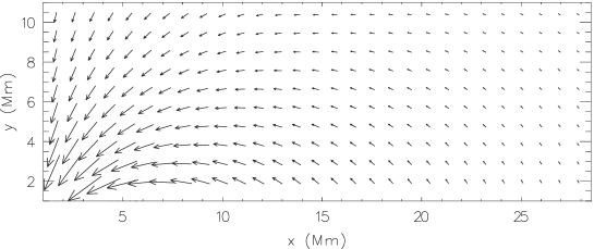
Figure 1.— Vectors of equilibrium magnetic field.

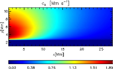
Figure 2.— Equilibrium profiles of the temperature along a fixed $x$ (top panel) and the Alfvén speed (bottom panel).

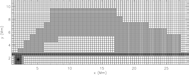
Figure 3.— Numerical blocks used in the numerical simulations for the case of $x_{\rm 0}=3$ Mm.

2.2. A model of the static solar atmosphere

We consider a model of the static ($\partial/\partial t=0$) solar atmosphere with an invariant coordinate $z$ ($\partial/\partial z=0$), but allow the $z$-components of velocity ($V_{\rm z}$) and magnetic field ($B_{\rm z}$) to vary with $x$ and $y$. In such 2.5 dimensional (2.5D) model, the solar atmosphere is in static equilibrium (${\bf V}_{\rm e}={\bf 0}$) with the force-free and current-free magnetic field defined by

$$\ (\nabla\times{\bf B}_{\rm e})\times{\bf B}_{\rm e}={\bf 0}\,,\hskip 11.38109pt\nabla\times{\bf B}_{\rm e}={\bf 0}\,.$$ (7)

Here the subscript _e corresponds to equilibrium quantities. We adopt a realistic magnetic flux-tube model originally developed for 3D by Low (1985), in which

$$\ {\bf B}_{\rm e}(x,y)=\nabla\times\left(A{\bf\hat{z}}\right)\,,$$ (8)

is an equilibrium magnetic field with ${\bf\hat{z}}$ being a unit vector along the $z$-direction and $A$ denoting the magnetic flux function given by

$$\ A(x,y)=\frac{x(y_{\rm ref}-b)^{2}}{(y-b)^{2}-x^{2}}B_{\rm ref}\,.$$ (9)

Here $b$ is a constant, which we choose and set equal to, $b=-5$ Mm, and $B_{\rm ref}$ is the magnetic field at the reference level, $y_{\rm ref}$ = 10 Mm.

Vectors of magnetic field, resulting from Eq. (8), are displayed in Fig. 1. The magnetic field is defined by the magnetic pole that is located at the point ($x$ = 0 Mm, $y$ = $-$5 Mm). Note that at a given altitude $y$ magnetic field is strongest around the line $x=0$ Mm, where it is essentially vertical. However, further out the magnetic field declines with larger values of $|x|$, revealing its curved structure. Such magnetic field corresponds to an isolated asymmetric magnetic arcade.

As a result of Eqs. (2) and (7), the pressure gradient is balanced by the force of gravity,

$$-\nabla p_{\rm e}+\varrho_{\rm e}{\bf g}={\bf 0}\,.$$ (10)

With the use of the ideal gas law given by Eq. (6) and the $y$-component of the hydrostatic pressure balance described by Eq. (10), we express the equilibrium gas pressure and mass density as

$$p_{\rm e}(y)=p_{\rm ref}~{}{\rm exp}\left(-\int_{y_{\rm r}}^{y}\frac{dy^{{}^{\prime}}}{\Lambda(y^{{}^{\prime}})}\right)\,,$$ (11)

$$\varrho_{\rm e}(y)=\frac{p_{\rm e}(y)}{g\Lambda(y)}\,,$$ (12)

where

$$\Lambda(y)=\frac{k_{\rm B}T_{\rm e}(y)}{mg}\ ,$$ (13)

is the pressure scale-height, and $p_{\rm ref}$ denotes the gas pressure at the reference level.

We adopt a realistic plasma temperature profile given by the semi-empirical VAL-C model (Vernazza et al. 1981) that is extrapolated into the solar corona, (Fig. 2, top panel). In our model, the temperature attains a value of about $5\times 10^{3}$ K at $y=1.5$ Mm and it increases to about $1.5\times 10^{6}$ K in the solar corona at $y=10$ Mm. Higher up in the solar corona the temperature is assumed to be constant. The temperature profile determines uniquely the equilibrium mass density and gas pressure profiles. At the transition region, which is located at $y\simeq 2.7$ Mm, $T_{\rm e}$ exhibits an abrupt jump (Fig. 2, top panel), but $\varrho_{\rm e}(y)$ and $p_{\rm e}(y)$ experience a sudden fall off with the atmospheric height (not shown).

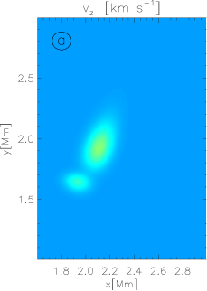
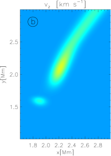
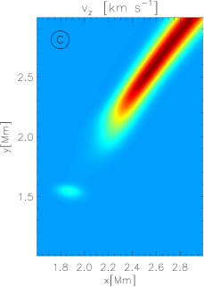
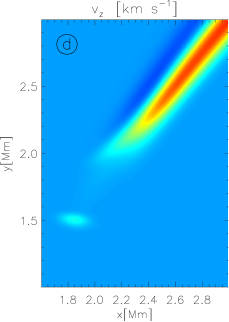
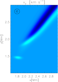
Figure 4.— Spatial profiles of the velocity $V_{\rm z}(x,y,t)$ near the point of initial perturbation for the case of $x_{\rm 0}=2$ Mm, $w_{\rm x}=0.1$ Mm at $t=5$ s, $t=8$ s, $t=11$ s, $t=14$ s, $t=18$ s and $t=21$ s, presenting propagation through the transition region and evolution of the initial pulse. A full-colour version of above figure and movie is available at www.pchmiel.republika.pl/store/Fig4.avi.

Figure 5.— The Alfvén speed, $c_{\rm A}$, along the magnetic line, which crosses the point $(x_{\rm 0},y_{\rm 0})=(2~{}$Mm$,1.75~{}$Mm$)$ (solid line) and the point $(x_{\rm 0},y_{\rm 0})=(3~{}$Mm$,1.75~{}$Mm$)$ (dashed line).

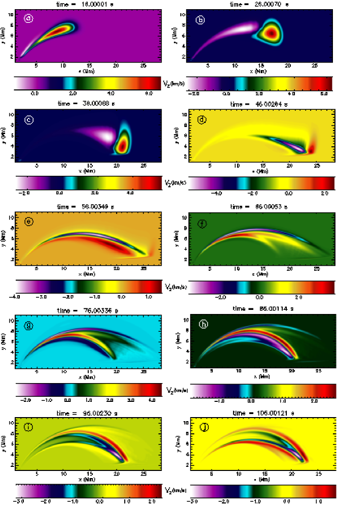
Figure 6.— Spatial profiles of transverse velocity $V_{\rm z}(x,y,t)$ for $x_{\rm 0}=2$ Mm, $w_{\rm x}=0.2$ Mm at $t=16$ s , $t=26$ s, $t=36$ s, $t=46$ s, $t=56$ s, $t=66$ s, $t=76$ s, $t=86$ s, $t=96$ s and $t=106$ s (from top-left to bottom-right). A full-colour version of above figure and movie is available at www.pchmiel.republika.pl/store/Fig6.avi.

In this model the Alfvén speed, $c_{\rm A}$, varies in both the $x$ and $y$ directions and it is expressed as follows:

$$c_{\rm A}(x,y)=\frac{|{\bf B}_{\rm e}(x,y)|}{\sqrt{\mu\varrho_{\rm e}(y)}}\,.$$ (14)

Its profile is displayed in Fig. 2 (bottom panel). Note that the Alfvén speed is non-isotropic; higher values are located near $x_{\rm 0}=0$ Mm, where the magnetic field is stronger, while $c_{\rm A}$ decreases with larger values of $x_{\rm 0}$. In the chromosphere $c_{\rm A}(x=0\,{\rm Mm},y=1.75\ {\rm Mm})$ is about $25$ km s^-1. The Alfvén speed rises abruptly through the solar transition region, reaching a value of $c_{\rm A}(x=0\,{\rm Mm},y=10\,{\rm Mm})=10^{3}$ km s^-1 (Fig. 2, bottom panel). The increase of $c_{\rm A}(x=0~{}{\rm Mm},y)$ with height results from a faster decrease of $\varrho_{\rm e}(y)$ than $B_{\rm e}(x=0\,{\rm Mm},y)$ with the atmospheric height.

3. Numerical simulations of MHD equations

To solve Eqs (1)-(6) numerically, we use the FLASH code (Fryxell et al. 2000; Lee & Deane 2009; Lee 2013), in which a third-order unsplit Godunov-type solver with various slope limiters and Riemann solvers as well as Adaptive Mesh Refinement (AMR) (MacNeice et al. 1999) are implemented. The minmod slope limiter and the Roe Riemann solver (e.g., Tóth 2000) are used. We set the simulation box as $(1\,{\rm Mm},28.5\,{\rm Mm})\times(1\,{\rm Mm},11\,{\rm Mm})$ and impose fixed in time boundary conditions for all plasma quantities in the $x$- and $y$-directions, while all plasma quantities remain invariant along the $z$-direction; however, note that both $V_{\rm z}$ and $B_{\rm z}$ differ from zero.

In our present work, we use a static, non-uniform grid with a minimum (maximum) level of refinement set to $4$ ($6$). We performed the grid convergence studies by refining this by a factor of two. As the numerical results remained essentially similar for the grid of maximum blocks levels 6 and 7, we adopted the former to get the results presented in this paper. Note that small size blocks of numerical grid occupy the solar transition region and the region located along Alfvén wave propagation path (Fig. 3), and every numerical block consists of $8\times 8$ identical numerical cells. This results in an excellent resolution of steep spatial profiles and greatly reduces the numerical diffusion in these regions.

3.1. Initial perturbations

We perturb initially (at $t=0$ s) the equilibrium described in Sec. 2.2 by a Gaussian pulse in the $z$-component of velocity given by

$$V_{\rm z}(x,y,t=0)=A_{\rm v}e^{-\frac{(x-x_{\rm 0})^{2}}{w_{\rm x}^{2}}-\frac{(y-y_{\rm 0})^{2}}{w_{\rm y}^{2}}}\,,$$ (15)

where $A_{\rm v}$ is the amplitude of the pulse, $(x_{\rm 0},y_{\rm 0})$ is its initial position and $w_{\rm x}$ and $w_{\rm y}$ denote its widths along $x$- and $y$-directions, respectively. We set and hold fixed $y_{\rm 0}=1.75$ Mm, $A_{\rm v}=3$ km s^-1 and $w_{\rm y}=0.1$ Mm, but allow $x_{\rm 0}$ and $w_{\rm x}$ to vary. This shows that Alfvén waves in our model are generated in the solar chromosphere just above the photosphere, which makes our model significantly different than that considered by Del Zanna et al. (2005) and Miyagoshi et al. (2004), who launched the initial pulses in the solar corona. Physical consequences of these differences are described in Sect. 4. It is clear that our more realistic model significantly extends the model considered by Del Zanna et al. (2005) and provides a platform to pursue the modelling of Alfvén wave phase-mixing in realistic solar atmosphere where an appropriate driver (dynamical phenomena in the solar chromosphere) is responsible for excitation of such waves.

Note that in our 2.5D model, the Alfvén waves decouple from magnetoacoustic waves and it can be described solely by $V_{\rm z}(x,y,t)$. As a result, the initial pulse triggers Alfvén waves that in the linear limit are approximately described by the following wave equation:

$$\frac{\partial^{2}V_{\rm z}}{\partial t^{2}}=c_{\rm A}^{2}(x,y)\frac{\partial^{2}V_{\rm z}}{\partial s^{2}}\,,$$ (16)

where $s$ is the coordinate along a magnetic field line.

4. Results of numerical simulations

We simulate small amplitude and impulsively excited Alfvén waves and investigate their propagation along magnetic field lines which are parallel to magnetic vectors shown in Fig. 1. This magnetic field configuration mimics an asymmetric solar arcade, which is more realistic than that considered by Del Zanna et al. (2005).

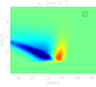
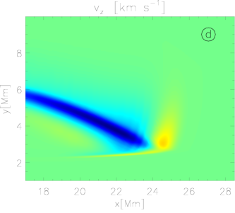
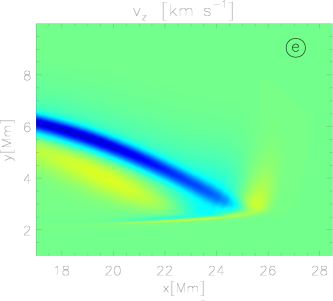
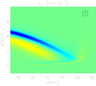
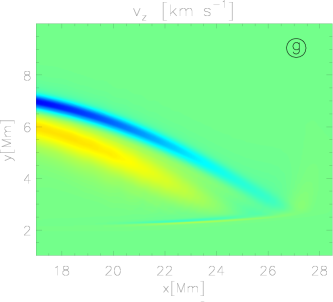
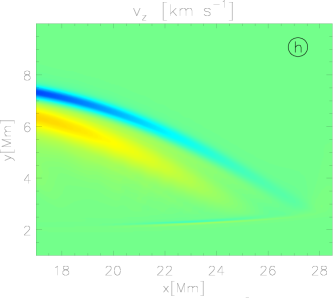
Figure 7.— Spatial profiles of transverse velocity $V_{\rm z}(x,y,t)$ for $x_{\rm 0}=2$ Mm, $w_{\rm x}=0.2$ Mm at $t=36$ s, $t=40$ s, $t=44$ s, $t=48$ s, $t=52$ s, $t=56$ s, $t=60$ s and $t=64$ s (from top-left to bottom-right), illustrating a partial reflection of Alfvén waves from the transition region.

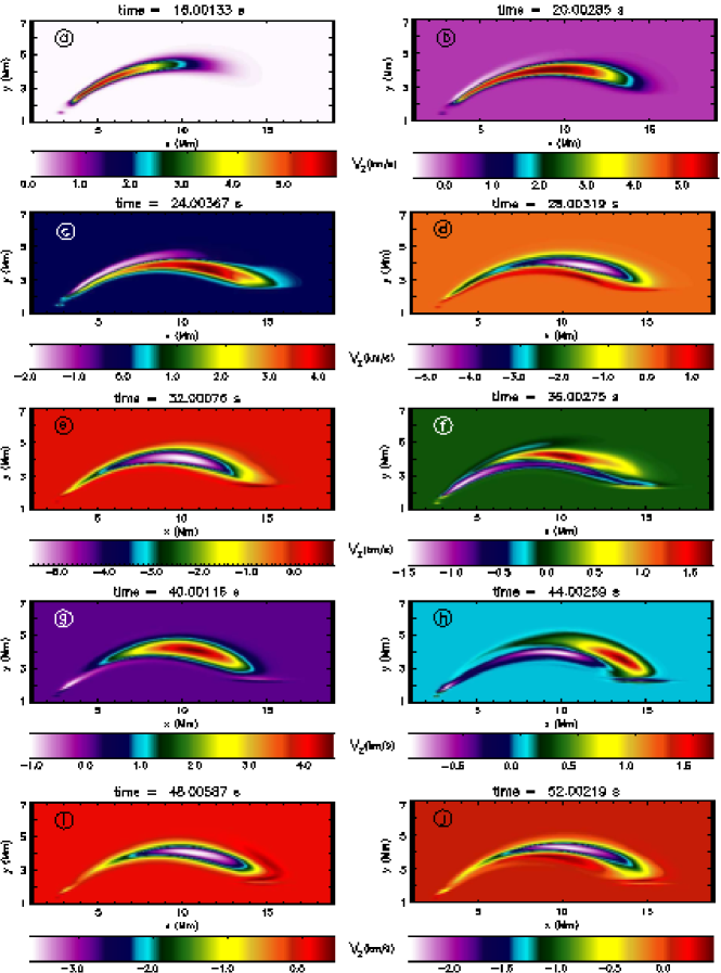
Figure 8.— Spatial profiles of transverse velocity $V_{\rm z}(x,y,t)$ for $x_{\rm 0}=3$ Mm, $w_{\rm x}=0.2$ Mm at $t=16$ s, $t=20$ s, $t=24$ s, $t=28$ s, $t=32$ s, $t=36$ s, $t=40$ s, $t=44$ s, $t=48$ s and $t=52$ s (from top-left to bottom-right). A full-colour version of above figure and movie is available at www.pchmiel.republika.pl/store/Fig8.avi.

Figure 9.— Vertical profiles of $V_{\rm z}(x=12\,{\rm Mm})$ for the case of $x_{\rm 0}=2\,{\rm Mm}$ (top panel) at $t=22$ s (solid line), $t=74$ s (dashed line) and $t=124$ s (dotted line), and $V_{\rm z}(x=9\,{\rm Mm})$ for the case of $x_{\rm 0}=3\,{\rm Mm}$ (bottom panel) at $t=20$ s (solid line), $t=40$ s (dashed line) and $t=60$ s (dotted line).

Figure 10.— Time-signatures of $V_{\rm z}$ for $w_{\rm x}=0.2$ Mm, $x_{\rm 0}=2$ Mm (top panel), $x_{\rm 0}=2.5$ Mm (middle panel) and $x_{\rm 0}=3$ Mm (bottom panel). Detection points are located at ($x=12$ Mm, $y=7$ Mm) (top panel), ($x=11$ Mm, $y=5.1$ Mm) (middle panel) and ($x=9$ Mm, $y=4.2$ Mm) (bottom panel).

4.1. Initial stage of wave propagation

The Gaussian pulse of initial perturbation in the $z$-component of velocity, described by Eq. (15), decouples into two moving in opposite directions pulses. The downwardly propagating pulse fades very fast, however the second one propagates through the chromosphere and transition region to the solar corona (Fig. 4).

As a result of several effects such as finite size of the Alfvén wave pulse, inclination of the magnetic field, and highly inhomogeneous Alfvén speed, $c_{\rm A}(x,y)$, the wave signal in our numerical simulations is deformed and elongated while passing in the arcade through the transition region. In Fig. 4, we observe the Alfvén waves reaching the transition region located at $y\simeq 2.7$ Mm, and accelerated due to a sudden increase of local Alfvén speed (panels $a$ and $b$). The wave signal penetrates gradually through the transition region. First, the initially circular wave profile is distorted to ellipsoidal shape because Alfvén speed slightly raise along the inclined magnetic field lines (Fig. 5), and next becomes significantly elongated above the transition region (Fig. 4, panel $c$) due to sudden increase of the Alfvén speed (Fig. 5).

This clearly shows that the upper part of the wave signal, propagating along the magnetic field lines, penetrates the solar corona earlier than the middle and bottom parts of the signal (Fig. 4, panel $b$). Moreover, the upper part of the wave follows along different (upper) magnetic field line than the right part of the wave that propagates over the lower magnetic field line, which results in deformation of the initial pulse and finally intensifies the phase-mixing that can be seen at the panels $d$ and $e$ of Fig. 4. Here, the upper part of the wave signal located at the upper magnetic field lines illustrated as a white patch (Fig. 4, panels $d$ and $e$) is in a different phase than the signal located at the lower magnetic field line, that already passed the transition region. This additional process of the wave deformation at the transition region significantly influences Alfvén wave propagation in the curved coronal arcades, introducing different phases of the wave signal in the arcade at beginning stage. Notice, that the Alfvén waves suffer from the partial reflection from the transition region and a small signal propagates backward into the solar surface, which can be spotted at $(x,y)\simeq(2$ Mm$,1.8$ Mm$)$ in Fig. 4, panels $e$ and $f$.

4.2. Different spatial positions of initial pulses

In our approach for a fixed value of $y_{0}$, the length and curvature of magnetic field lines vary with $x_{\rm 0}$. For a smaller value of $x_{\rm 0}$ a magnetic line is longer, more curved, and less inclined to the horizontal direction (Fig. 1) as well as Alfvén speed $c_{\rm A}(x,y)$ experiences a larger structuring there (Fig. 2, bottom panel). While a larger value of $x_{\rm 0}$ corresponds to a shorter, less curved and more inclined magnetic field lines as well as less varying $c_{\rm A}(x,y)$. Here, we consider two different cases of initial pulse position: $x_{\rm 0}=2$ Mm and $x_{\rm 0}=3$ Mm. In the first case, the Alfvén waves propagate higher up along longer and more curved magnetic field lines. However, in the case of $x_{\rm 0}=3$ Mm, the inclination of magnetic field lines to $x$-axis is much larger and this results in approximately two times smaller size of the arcade with less curved field lines. In Fig. 5, we notice that $c_{\rm A}(s)$ varies less along the magnetic field line, $s$, for a small arcade, reaching a value of $2$ Mm s^-1 (dashed line), while for a large arcade it attains $2.4$ Mm s^-1 (solid line). Here, a value of $s=0$ corresponds to the point at which the initial perturbation was launched, $(x_{\rm 0},y_{\rm 0})$, equal to $(2$ Mm$,1.75$ Mm$)$ for the large arcade (solid line) and $(3$ Mm$,1.75$ Mm$)$ for the small arcade (dashed line).

4.2.1 Large arcade

Our numerical results are presented in Fig. 6, which illustrates spatial profiles of Alfvén waves generated by the initial Gaussian pulse given by Eq. (15). This pulse triggers counter-propagating Alfvén waves (e.g., Murawski & Musielak 2010). The wave that propagates downward enters a region of small Alfvén speed, which results from high mass density there. The presented results show that the evolution of the downwardly propagating waves (Fig. 4) is much less dynamic than the evolution of Alfvén waves that already reach the upper regions of the solar atmosphere.

The upwardly propagating Alfvén waves, reaching the transition region, accelerate due to increase of local Alfvén speed (Fig. 2, bottom panel, and Fig. 5, solid line) and penetrate into the solar corona. In Fig. 6, panel $a$, the wave signal arrived to the level $y=9$ Mm. At $t=26$ s (panel $b$), the Alfvén waves are at the apex while fanning its spatial profile as a result of diverging magnetic field lines (Fig. 1), and the spatial variation of the Alfvén speed (Fig. 2, bottom panel). This process becomes even more pronounced in time as the Alfvén waves penetrate the regions of more diverged field lines. Behind the Alfvén wave signal, there is visible fanning of a negative value of $V_{\rm z}$ (violet-white patch), that is a remnant after the Alfvén wave passing through the plasma medium (Murawski & Musielak 2010).

Now, the violet patch seen in Fig. 6 becomes elongated and it contains a white subregion located at $x=12$ Mm, $y=7$ Mm (panel $b$). This white subregion corresponds to negative ($V_{\rm z}\approx-2.1$ km s^-1) values of transversal velocity while nearby laying positive velocity ($V_{\rm z}\approx 6.4$ km s^-1) region is represented by a red patch. This results from the finite-size of the initial pulse whose left and right-sides have to pass significantly different distances, because the magnetic field line along the left-side path is longer than the magnetic field line along the right-side in the considered arcade. Moreover, a strong fanning of the wave signal spatial profile is a consequence of the Alfvén speed, $c_{\rm A}(x,y)$, which attains different values along different magnetic interfaces (Fig. 2, bottom panel). At $t=36$ s, the already downwardly propagating Alfvén waves reach the transition region (panel $c$) and they undergo partial reflection from this region.

The resulting wave reflection is well seen at the consecutive moments of time, e.g., at $t=46$ s (panel $d$) and at $t=56$ s (panel $e$), respectively. However, at later moments of time the Alfvén waves profiles become more complicated; we can notice a partial reflection of the wave signal with negative value of $V_{\rm z}$, illustrated by narrow elongated violet-white patch (panels $e$ and $f$). At $t=66$ s the Alfvén waves reflect again at the left side, near $x_{\rm 0}=2$ Mm and propagate with positive phase velocity (red patch) at $t=76$ s with amplitude $V_{\rm z}\approx 4.2$ km s^-1 in right direction. We observe a long narrow signal seen as a red patch, which reaches the transition region near $x_{\rm 0}=21$ Mm at $t=86$ s (panel $h$). Reflections of the Alfvén waves are well seen at $t=86$ s (panel $h$) and $t=96$ s (panel $i$) as violet-white patches near $x_{\rm 0}=21$ Mm. Such reflections result in complex Alfvén waves spatial profiles. We provide details on the partial reflection in Sect. 4.4, where we evaluate the corresponding reflection coefficient.

Fig. 7 presents in some details the Alfvén waves reflection. The arriving waves (panel $a$, red patch) hit the transition region and start reflecting in there, decreasing its amplitude, which is well seen in consecutive moments of time. In panel $b$, the reflected, backwardly propagating wave is illustrated by a violet-white patch, superimpose on the arriving negative phase waves. The effect of superimposition of the wave signals is significant, because of fanning of the wave spatial profiles, which are a consequence of large arcade, where Alfvén speed gradient and diverged magnetic field lines are large. At later moments of time (panels $e$ to $h$), we also see the evolution of the lagging wave signals reflected from the transition region as a red patch under the backward propagating main signal (violet-white patch).

Note that there is clearly seen small partially non-reflected (transmitted) Alfvén waves propagating downwardly into the solar surface under the transition region. These waves are in phase and their amplitude is about $1$ km s^-1.

It is worth to compare our results to those previously obtained by Del Zanna et al. (2005), who considered an isothermal symmetric solar arcade with the transverse signal undergoing reflection from the transition region. In our non-isothermal asymmetric arcade, the numerical results show how the Alfvén wave pulse is widened by the diverged magnetic field lines, becomes gradually reflected in the transition region, and creates a non-regular structure of the reflected wave signal (see Fig. 6, bottom-right). Later on, the diverged magnetic field configuration, inhomogeneous Alfvén speed, difference of magnetic field lengths and the reflected waves interaction with the ongoing wave train complicates even more the spatial velocity profiles in the arcade.

4.2.2 Short arcade

Spatial profiles of Alfvén waves, which result from the initial Gaussian pulse given by Eq. (15), with $x_{\rm 0}=3$ Mm and $w_{\rm x}=0.2$ Mm are presented in Fig. 8. Initial pulse triggers the counter-propagating Alfvén waves in a comparatively less curved magnetic arcade. In this case, process of initial deformation of the wave pulse during propagation throughout the transition region is more effective because magnetic field lines are more horizontal than in the case of $x_{\rm 0}=3$ Mm. The upper part of the signal propagates earlier than the rest of the pulse and strongly influences on phase-mixing. On the other hand, a smaller arcade results in less diverged magnetic lines and less ${\bf\nabla}c_{\rm A}(x,y)$, that in consequence significantly reduces the fanning process of the wave signal.

Such a smaller arcade causes that a wave signal ranges all arcade region. At $t=20$ s (panel $b$) and later on, the outer edge of the arcade with its large length clearly reveals a phase difference of transversal wave velocity profiles as compared to the same in the core of the arcade. We observe several wave signal reflections from the transition region in Fig. 8. The violet-white patch in panels $d$ and $e$ represents reflected Alfvén waves that propagate to the left-hand side. When they reach the transition region near $x=3$ Mm, they become reflected and propagate again into the right-hand side (panels $f$ and $g$) to suffer reflection once again near $x=16$ Mm, which is clearly seen at $t=44$ s (panel $h$), and go back into $x=3$ Mm (panels $i$ and $j$). It should be noted that the initial pulse-width was assumed to be the same as in the case of $x_{\rm 0}=2$ Mm (Fig. 6).

4.2.3 Comparison

In the presented vertical cross-sections of the Alfvén wave profiles, we observe difference in wave propagation for large (Fig. 9, top panel) and small arcades (Fig. 9, bottom panel). The cross-section for the case of $x_{\rm 0}=2$ Mm ($x_{\rm 0}=3$ Mm) shows the region near the apex of the arcade, $x=12$ Mm ($x=9$ Mm), and three moments of time, when the wave signal passing the apex: $t=22$ s ($t=20$ s), $t=72$ s ($t=40$ s) and $t=124$ s ($t=60$ s), that are illustrated in the top (bottom) panel of Fig. 9 by solid, dashed and dotted line, respectively. The main difference between these two cross-sections is a compact shape of the Alfvén wave in the short arcade during all three moments of time in comparison to the large arcade. This is a result of less diverged magnetic lines, which spread the signal up to width equal $5$ Mm in the case of $x_{\rm 0}=2$ Mm, while in the case of $x_{\rm 0}=3$ Mm a pulse width is about $2$ Mm.

We also find a difference in negative phase amplitudes. The Alfvén wave cross-section in the large arcade (Fig. 9, top panel) already after one period exhibits minima with negative values of $V_{\rm z}$ accompanying the main wave signal. At $t=72$ s (dashed line), the first opposite-sign phase with amplitude $V_{\rm z}\simeq-2.2$ km s^-1 at $y\simeq 8.8$ Mm is a part of the elongated main wave signal still following into the transition region located near $x=2$ Mm to suffer reflection (Fig. 6, panel $g$, upper violet white patch), while the second opposite-sign phase with amplitude $V_{\rm z}\simeq-0.8$ km s^-1 at $y\simeq 6.6$ Mm is a signal that lags behind the main Alfvén signal, well seen in panel $g$ of Fig. 6 (lower violet patch). In later moment of time, at $t=124$ s (dotted line) the negative value of $V_{\rm z}$ has a similar form, however the amplitudes are $V_{\rm z}\simeq-1.4$ km s^-1 at $y\simeq 7.6$ Mm and $V_{\rm z}\simeq-0.8$ km s^-1 at $y\simeq 6.7$ Mm.

In the case of a short arcade (Fig. 9, bottom panel), for which divergence of magnetic lines and the gradient of $c_{\rm A}$ are smaller, the opposite-sign phases at the cross-section states only $0.9$% of the main wave signal amplitude equal to $V_{\rm z}\simeq 5.6$ km s^-1 at $t=20$ s (solid line), $7$% of the amplitude equal to $V_{\rm z}\simeq 3.8$ km s^-1 at $t=40$ s (dashed line) and $15.2$% of the amplitude equal to $V_{\rm z}\simeq 2.5$ km s^-1 at $t=60$ s (dotted line).

Figure 10 illustrates the time-signatures of $V_{\rm z}$ collected at points near the apex of each arcade. The time-signatures for cases of $x_{\rm 0}=2$ Mm, $x_{\rm 0}=2.5$ Mm and $x_{\rm 0}=3$ Mm are presented in top, middle and bottom panels, respectively. We set the detection point for the case of $x_{\rm 0}=2$ Mm to be at ($x=12$ Mm, $y=7$ Mm), for the case of $x_{\rm 0}=2.5$ Mm to be at ($x=11$ Mm, $y=5.1$ Mm) and for the case of $x_{\rm 0}=3$ Mm at ($x=9$ Mm, $y=4.2$ Mm). Time-signatures for smaller arcades ($x_{\rm 0}=2.5$ Mm and $x_{\rm 0}=2$ Mm) have a regular harmonic shape, but the time-signature for the large arcade exhibits action on fanning process that results in superimposition of incoming and reflected wave signals in $V_{\rm z}$ and finally in non-regular shape of $V_{\rm z}$ oscillations. Note that the amplitude of the Alfvén waves decays with time and that $V_{\rm z}$ oscillates with its characteristic wave period equal to $P=50.7$ s for $x_{\rm 0}=2$ Mm, $P=27.2$ s for $x_{\rm 0}=2.5$ Mm and $P=20.4$ s for $x_{\rm 0}=3$ Mm. These different wave periods result from the different arcade lengths and different Alfvén speeds along the corresponding magnetic lines for $x_{\rm 0}=2$ Mm, $x_{\rm 0}=2.5$ Mm and $x_{\rm 0}=3$ Mm.

Figure 11.— Travel time vs. the horizontal initial position, $x_{\rm 0}$, along the magnetic field line crossing the point $(x_{\rm 0},1.75$ Mm$)$.

We calculate a travel time of the Alfvén waves, $t_{\rm t}$, for the first bounce along few magnetic field lines, which cross the given point $(x_{\rm 0},y_{\rm 0})$,

$$t_{\rm t}=\int_{0}^{l}\frac{ds}{c_{\rm A}(s)}\,.$$ (17)

Here, a coordinate along the magnetic line has the value of $s=0$ at $(x_{\rm 0},y_{\rm 0})$, while for $s=l$ the magnetic line ends at the transition region, $y=2.75$ Mm. In Fig. 11 the travel time is displayed depending on the initial point $x_{\rm 0}$. Its value gradually decreases with $x_{\rm 0}$ from $t_{\rm t}\simeq 39$ s at $x_{\rm 0}=2$ Mm, reaching $t_{\rm t}\simeq 26$ s at $x_{\rm 0}=3$ Mm. Because of almost linear decrease of the magnetic field length from $l=23.4$ Mm at $x_{\rm 0}=2$ Mm up to $l=11.6$ Mm at $x_{\rm 0}=3$ Mm (not shown), these results show that the time of the Alfvén wave traveling along longer magnetic field lines is much bigger, than for shorter magnetic lines. This effect is especially important in case of the large arcade, where the travel time falls off rapidly, contributing to the wave signal profile fanning.

Our results show the complex picture of Alfvén waves caused by wave reflection from the transition region, and difficulties in direct studies of the interaction of counter-propagating waves in the asymmetric solar arcade. Because of these difficulties, we instead focus on evaluating a global attenuation time. This allows us to investigate integrally the attenuation processes affecting the transverse waves, like interactions of the counter-propagating waves, partial wave reflection from the transition region, and the wave energy leakage along a curved magnetic field lines of the arcade.

Figure 12.— The ratio of the attenuation time over wave period, $\tau$/$P$, vs. pulse width $w_{\rm x}$ for the case of $x_{0}=2$ Mm (top panel) and $x_{0}=3$ Mm (bottom panel).

Figure 13.— The value of arcade full width at half maximum (FWHM) vs. $x_{\rm 0}$ for the chosen $x=11$ Mm.

Figure 14.— The reflection coefficient, $C_{\rm r}$, vs. $x_{\rm 0}$.

4.3. Different pulses width

For a wider initial pulse, $w_{\rm x}$, the process of phase-mixing becomes stronger. The reason is that both sides of such pulse experience a larger phase difference due to a larger difference in field lines curvatures on both magnetic interfaces and pulse deformation process in the transition region as compared to a narrower pulse. Hence, for the wider pulse more strongly Alfvén waves propagation is affected.

Basing on data signal of $V_{\rm z}$ collected at point ($x=12$ Mm, $y=7$ Mm) for the case of longer arcade ($x_{\rm 0}=2$ Mm) and ($x=9$ Mm, $y=4.2$ Mm) for the case of shorter arcade ($x_{\rm 0}=3$ Mm), we evaluate a wave period $P$ using fast Fourier transform method and an attenuation time $\tau$. The ratio of attenuation time $\tau$ to a wave period $P$ with respect to the width of the initial pulse is presented in Fig. 12, which shows that $\tau/P$ first increases for small values of $w_{\rm x}$ but then falls off slightly with $w_{\rm x}$.

When we look at the individual $\tau/P$ versus the pulse width profiles of the two types of arcades, they exhibit a similar trend that is some increment up to a certain pulse width and then decrement. In the case of the considered geometry of more curved and larger magnetic arcade, the $\tau/P$ first increases up to $100$ km pulse width (Fig. 12, top panel), which means that up to this limit of the pulse width the attenuation of Alfvén waves decreases in the arcade.

Similarly in the case of the considered geometry of less curved and smaller magnetic arcade, the $\tau/P$ first increases up to $400$ km pulse width (Fig. 12, bottom panel), which means that up to this limit of pulse width the attenuation of Alfvén waves decreases in the arcade. For $w_{\rm x}>400$ km, the $\tau/P$ decreases (Fig. 12, bottom panel), which is the signature of the increment in the wave attenuation. In other words, for the Alfvén waves launched with the pulse widths larger than $400$ km, the generated long wavelengths do not fit within the considered loop geometry and the wave leakage again causes a wave attenuation (Gruszecki et al. 2007).

It is also found that the attenuation of the Alfvén waves is smaller (larger the attenuation time with respect to the wave period) in the more curved and larger magnetic arcades ($x_{\rm 0}=2$ Mm), while it is larger (smaller the attenuation time with respect to the wave period) in the case of the less curved and comparatively smaller arcades ($x_{\rm 0}=3$ Mm). We found $\tau/P=1.75$ s for the core of $x_{\rm 0}=2$ Mm and $\tau/P=1.89$ s for $x_{\rm 0}=3$ Mm, for $w_{\rm x}=0.2$ Mm.

The arcade full width at half maximum (FWHM) dependence on the position of initial pulse $x_{\rm 0}$, and in consequence on a size of the arcade, is shown in Fig. 13, which clearly illustrates that a smaller arcade (bigger $x_{\rm 0}$) has a smaller width (FWHM); a smaller arcade consists of weakly diverged magnetic field lines.

If one considers the phase-mixing to be the only candidate for the wave dissipation (e.g., Heyvaerts & Priest 1983), then the strong phase-mixing in the more curved and larger arcades (cf., Fig. 6) must cause a greater attenuation as compared to the less strong phase-mixing in the less curved and smaller arcades (cf., Fig. 8). Nevertheless, the simulation results demonstrate a more complicated scenario of the wave attenuation, which simply implies that the phase-mixing may not be the only candidate responsible for the wave attenuation; actually, the magnetic field configuration and plasma properties of the arcade such as a spatial profile of the Alfvén speed, strength and dimension of the pulse, and the structure of the transition region, all play the vital role in this phenomenon.

4.4. Partial reflection from the transition region

Decay of the Alfvén wave amplitude results from the wave energy leakage caused by the curvature and divergence of magnetic field lines, inhomogeneous Alfvén speed $c_{\rm A}(x,y)$ and a partial penetration of Alfvén wave signal into the chromosphere (Gruszecki et al. 2007). We clearly observe in our simulation that Alfvén waves experience partial reflection from the transition region and Alfvén waves signal penetrates into solar atmospheric layers under the transition region (Figs. 6 and  7, panels $d-h$). The amplitude of the waves penetrating into the lower region of the atmosphere drops from about $V_{\rm z}=1$ km s^-1 at $t=48$ s just under the transition region (Fig. 7, panel $d$), through $V_{\rm z}=0.5$ km s^-1 after about $16$ s (Fig. 7, panel $h$) and finally disappears. We can evaluate the reflection coefficient,

$$C_{\rm r}=\frac{A_{\rm r}}{A_{\rm i}}\,,$$ (18)

where $A_{\rm i}$ ($A_{\rm r}$) is the amplitude of the incident (transmitted) waves. Substituting $A_{\rm i}=6$ km s^-1 and $A_{\rm r}=4.01$ km s^-1 into the above formula we get $C_{\rm r}=0.668$, which means that $66.8$% of the waves amplitude became reflected in the transition region and $33.2$% was transmitted into lower atmospheric layers. The reflection coefficient, $C_{\rm r}$, vs. initial pulse position $x_{\rm 0}$ for the first reflection from the transition region is presented in Fig. 14. We expect that the amplitude of the wave signal reflected in the transition region is smaller for Alfvén waves in larger inclined magnetic field lines, which corresponds to larger values of $x_{\rm 0}$.

In the case of the largely curved arcades, the lateral leakage of the Alfvén wave energy may also be largely dominant as compared to the one associated with less curved arcades (Gruszecki et al. 2007). The partial Alfvén wave reflection results from a steep gradient of Alfvén speed in the transition region because of a significant mass density drop in this region of the solar atmosphere.

It must be also noted that in case of linear Alfvén waves generated by small initial velocity pulses, $V_{\rm z}=3$ km s^-1 with the maximum amplitude reaching only $V_{\rm z}\approx 6$ km s^-1, there are no associated density variations.

5. Summary and Conclusions

To determine the role played by Alfvén waves in the coronal heating and solar wind acceleration, a number of authors investigated physical processes responsible for the excitation and attenuation of Alfvén waves in the solar atmosphere (e.g., Priest 1982; Ofman & Davila 1995; Ofman 2002; Miyagoshi et al. 2004; Dwivedi & Srivastava 2006; Ofman & Wang 2007; Chmielewski et al. 2013, and references therein). In general, Alfvén waves are difficult to dissipate their energy and possible mechanisms involve the collisional dissipative agents, such as viscosity and resistivity, or non-classical plasma processes, such as mode-coupling and phase-mixing (cf., Heyvaerts & Priest 1983; Nakariakov et al. 1997; Zaqarashvili et al. 2006; Dwivedi & Srivastava 2006, and references there). Overall, the collisional dissipative processes are found to be less important for the Alfvén wave dissipation than the non-classical plasma processes, especially phase-mixing (e.g., Nakariakov et al. 1997). Extensive observational searches were performed to find signatures of the Alfvén waves dissipation in the solar corona (e.g., Banerjee et al. 1998; Harrison et al. 2002; O’Shea et al. 2005; Bemporad et al. 2012, and references therein). However, as of today, there is no convincing observational evidence for the existence of Alfvén waves dissipation in the solar atmosphere.

In this paper, we simulated impulsively generated Alfvén waves in a stratified and magnetically confined solar arcade with the VAL-C temperature profile (Vernazza et al. 1981) as an initial realistic plasma condition in the curved magnetic field topology. Asymmetric solar magnetic arcades and the Alfvén waves propagation in these arcades were modeled by the time-dependent MHD equations that were solved numerically by the publicly available FLASH code (Lee & Deane 2009). We analyzed the effects of changing the horizontal position of the initial pulse and its width on the Alfvén wave propagation in the asymmetric solar arcade, the Alfvén wave deformation and phase-mixing resulting from inhomogeneous Alfvén wave velocity, and different lengths and divergence of magnetic field lines, and the partial wave reflection in the solar transition region.

We found that the more curved and larger arcade, then the stronger attenuation of the Alfvén waves. Our results also demonstrated attenuation of Alfvén waves resulted from the curvature and divergence of magnetic field lines, inhomogeneous Alfvén wave velocity, partial reflection in the solar transition region, as well as the decrement of the attenuation time of Alfvén waves for wider initial pulses in the given magnetic configuration of various types of arcades. Moreover, our numerical simulations also showed that Alfvén waves, which are partially reflected in the solar transition region return to the solar chromosphere as slowly downward propagating Alfvén waves.

The approach presented in this paper allowed us to investigate the effects caused by trains of Alfvén waves propagating in our arcade model as a result of the wave reflection in the solar transition region. Our results clearly show that the pulse deformation process in the transition region has a strong influence on the Alfvén waves propagation and on the wave damping in the curved magnetic field of the solar arcade together with the asymmetric magnetic field configuration, the plasma properties of the arcade, the horizontal size of the pulse, and the structure of the solar transition region.

In the previous work, Nakariakov et al. (1999) investigated the transverse oscillations of EUV loops as observed by the Transition Region and Coronal Explorer (TRACE), and demonstrated that the damping time was three times longer than the period of oscillations. They considered kink oscillations of coronal loops and their damping caused by non-classical viscosity and resistivity. Then, Ofman et al. (2002) showed that the dissipation of Alfvén waves due to chromospheric wave leakage was not sufficient to describe such fast damping of the observed transversal oscillations in the solar atmosphere. Finally, Del Zanna et al. (2005) demonstrated that dissipation of Alfvén pulses within their coronal arcade led to a change in the local Alfvén speed at various heights, and depending upon various localized conditions that determine the observed damping of these transverse oscillations.

In our work, the damping/attenuation time of the Alfvén waves are almost three times longer than that computed in both the longer and shorter arcades for a given pulse-width of 0.2 Mm. It should be noted that this damping time is due to the Alfvén wave dissipation caused by the phase mixing. The ratio of attenuation time and wave period is almost the same to what is observed for the transverse wave dissipation in coronal loops. An important point that must be mentioned is that transverse kink waves with their radial velocity perturbations in the cylindrical thin tube geometry (Roberts 2000) are different than Alfvén waves studied in this paper, which are essentially azimuthal. Nevertheless, there is a similar dissipation mechanism (e.g., phase-mixing) that may work for these two types of waves; its efficiency highly depends on the localized plasma, magnetic field configuration, nature of wave drivers, and Alfvén velocity, and others (see Ofman et al. 2002, 2007; Del Zanna et al. 2005). Therefore, our parametric studies presented in this provide some likely physical scenario for dissipation of Alfvén waves through phase-mixing.

Finally, we would like to point out that our approach is significantly different from that developed by Del Zanna et al. (2005), who considered a symmetric coronal arcade, which was embedded in the isothermal plasma with the constant (in time) temperature specified by the hyperbolic tangent profile, and designed it in such a way that it described short lived Alfvén waves in post flare settings. Similarly, Miyagoshi et al. (2004) simulated Alfvén waves that were excited by perturbations imposed in the solar corona. By using our more realistic arcade model with the asymmetric magnetic field configuration, we were able to explore different physical aspects of the Alfvén wave propagation than those studied in the past. Essentially, our model significantly generalizes the model originally considered by Del Zanna et al. (2005) and by Miyagoshi et al. (2004). Nevertheless, further improvements of our model are possible and it is our hope that they would lead to even better understanding of the inherent physical complexity of phase-mixing process and its role in heating of the solar corona by Alfvén wave dissipation.

References

- (1)
- (2) Arregui, I., Oliver, R., & Ballester, J. L. 2004, ApJ, 602, 1006
- (3) Banerjee, D., Teriaca, L., Doyle, J. G., & Wilhelm, K. 1998, A&A, 339, 208
- (4) Bemporad, A., & Abbo, L. 2012, ApJ, 751, 110
- (5) Biskamp, D., & Welter, H. 1989, Sol. Phys., 120, 49
- (6) Čadez, V. M., Oliver, R., & Ballester, J. L. 1994, A&A, 282, 934
- (7) Chmielewski, P., Srivastava, A. K., Murawski, K., & Musielak, Z. E. 2013, MNRAS, 428, 4
- (8) Del Zanna, L., Schaekens, E., and Velli, M. 2005, A&A, 431, 1095
- (9) Díaz, A. J., Zaqarashvili, T., & Roberts, B. 2006, A&A, 455, 709
- (10) Dwivedi, B. N., & Srivastava, A. K. 2006, Sol. Phys., 237, 143
- (11) Fryxell, B., Olson, K., Ricker, P., et al. 2000, ApJS, 131, 273
- (12) Gruszecki, M., Murawski, K., Selwa, M., & Ofman, L. 2006, A&A, 460, 887
- (13) Gruszecki, M., Murawski, K., Solanki, S. K., & Ofman, L. 2007, A&A, 469, 1117
- (14) Gruszecki, M., & Nakariakov, V. M. 2011, A&A, 536, A68
- (15) Harrison, R. A., Hood, A. W., & Pike, C. D. 2002, A&A, 392, 319
- (16) Heyvaerts, J., & Priest, E. R. 1983, A&A, 117, 220
- (17) Innes, D. E., McKenzie, D. E., & Wang, T. 2003, Sol. Phys., 217, 267
- (18) Lee, D. 2013, J. Comp. Phys., 243, 26
- (19) Lee, D., & Deane, A. E. 2009, J. Comp. Phys., 228, 952
- (20) Low, B.C. 1985, ApJ, 293, 31
- (21) MacNeice, P., Spicer, D. S., & Antiochos, S. 1999, 8th SOHO Workshop: Plasma Dynamics and Diagnostics in the Solar Transition Region and Corona, 446, 457
- (22) McKenzie, D. E., & Savage, S. L. 2009, ApJ, 697, 1569
- (23) Mikic, Z., Schnack, D. D., & van Hoven, G. 1989, ApJ, 338, 114
- (24) Miyagoshi, T., Yokoyama, T., & Shimojo, M. 2004, PASJ, 56, 207
- (25) Murawski, K., & Musielak, Z. E. 2010, A&A, 518, A37
- (26) Nakariakov, V. M., Roberts, B., & Murawski, K. 1997, Sol. Phys., 175, 93
- (27) Oliver, R., Hood, A. W., & Priest, E. R. 1996, ApJ, 461, 424
- (28) O’Shea, E., Banerjee, D., & Doyle, J. G. 2005, A&A, 436, L43
- (29) Ofman, L., & Davila, J. M. 1995, J. Geophys. Res., 100, 23427
- (30) Ofman, L. 2002, ApJ, 568, L135
- (31) Ofman, L., & Wang, T. 2007, AGU Fall Meeting Abstracts, 2
- (32) Priest, E. R. 1982, Dordrecht, Holland ; Boston : D. Reidel Pub. Co. ; Hingham,, 74P
- (33) Rial, S., Arregui, I., Terradas, J., Oliver, R., & Ballester, J. L. 2010, ApJ, 713, 651
- (34) Robert, B., 2000, SoHO , 4.
- (35)
- (36) Selwa, M., Murawski, K., Solanki, S. K., Wang, T. J., & Tóth, G. 2005, A&A, 440, 385
- (37) Selwa, M., Solanki, S. K., Murawski, K., Wang, T. J., & Shumlak, U. 2006, A&A, 454, 653
- (38) Toth, G. 2000, J. Comp. Phys., 161, 605
- (39) Vernazza, J. E., Avrett, E. H., & Loeser, R. 1981, ApJS, 45, 635
- (40) Verwichte, E., Nakariakov, V. M., Ofman, L., & Deluca, E. E. 2004, Sol. Phys., 223, 77
- (41) Verwichte, E., Foullon, C., & Van Doorsselaere, T. 2010, ApJ, 717, 45
- (42) Zaqarashvili, T. V., Oliver, R., & Ballester, J. L. 2006, A&A, 456, L13