Adaptive Learning in Cartesian Product of Reproducing Kernel Hilbert Spaces

Abstract

We propose a novel adaptive learning algorithm based on iterative orthogonal projections in the Cartesian product of multiple reproducing kernel Hilbert spaces (RKHSs). The task is estimating/tracking nonlinear functions which are supposed to contain multiple components such as (i) linear and nonlinear components, (ii) high- and low- frequency components etc. In this case, the use of multiple RKHSs permits a compact representation of multicomponent functions. The proposed algorithm is where two different methods of the author meet: multikernel adaptive filtering and the algorithm of hyperplane projection along affine subspace (HYPASS). In a certain particular case, the ‘sum’ space of the RKHSs is isomorphic to the product space and hence the proposed algorithm can also be regarded as an iterative projection method in the sum space. The efficacy of the proposed algorithm is shown by numerical examples.

I Introduction

Using reproducing kernels for nonlinear adaptive filtering tasks has widely been investigated [1, 2, 3, 4, 5, 6, 7, 8, 9, 10, 11]. See, e.g., [12, 13, 14, 15, 16, 17, 18, 19, 20, 21] for the theory and applications of reproducing kernels. The author has proposed and studied multikernel adaptive filtering, using ‘multiple’ kernels [22, 23, 24]. Different approaches using multiple kernels have also been proposed subsequently. Pokharel et al. have proposed a mixture-kernel approach [25], and Gao et al. have proposed convex-combinations of kernel adaptive filters [26]. Tobar et al. have proposed a multikernel least mean square algorithm for vector-valued functions [27]. Multikernel adaptive filtering is effective particularly in the following situations.

1. The unknown system to be estimated contains multiple components with different characteristics such as (i) linear and nonlinear components and (ii) high- and low- frequency components. See [28, 29, 30, 31].

2. An adequate kernel is unavailable because (i) the amount of prior information about the unknown system is limited, and/or (ii) the unknown system is time-varying and so is the adequate kernel for the system.

The situation (b) has mainly been supposed in [22, 23, 24]. Use of many, say fifty, kernels has been investigated and kernel-dictionary joint-refinement techniques have been proposed based on double regularization with a pair of block $\ell_{1}$ norms [32, 33]. Our primal focus in the current study is on the situation (a) in which the use of multiple kernels is expected to allow a compact representation of the unknown system.

Separately from the study of multikernel adaptive filtering, the author has proposed an efficient single-kernel adaptive filtering algorithm named hyperplane projection along affine subspace (HYPASS) [34, 35]. The HYPASS algorithm is a natural extension of the naive online $R_{\rm reg}$ minimization algorithm (NORMA) proposed by Kivinen et al. [1]. NORMA seeks to minimize a risk functional in terms of a nonlinear function by using the stochastic gradient descent method in a reproducing kernel Hilbert space (RKHS). This approach builds a dictionary (the set of basic nonlinear functions to generate an estimate of the unknown system) by using all the observed data. This implies that the dictionary size grows with the number of data observed. As a remedy for this issue, a simple truncation rule has been introduced [1]. It would be more realistic to build a dictionary in a selective manner based on some criterion to evaluate the novelty of a new datum; simple criteria include Platt’s criterion [36], the approximate linear dependency [2], and the coherence criterion [7]. Introducing one of those criteria to NORMA raises another issue: if a new datum is regarded to be not sufficiently novel and does not enter into the dictionary, then this observed datum is simply discarded and makes no contributions to estimation even though it can be informative enough to adjust the coefficients. Moreover, the coefficient of each dictionary element is updated only when that element enters into the dictionary. The HYPASS algorithm systematically eliminates this limitation by enforcing the update direction to lie in the dictionary subspace which is spanned by the dictionary elements. It has been extended to a parallel-projection-based algorithm [37, 35]. HYPASS includes the method of Dodd et al. [38] and the quantized kernel LMS (QKLMS) [39] as its particular case. There are a similarity, and also a considerable dissimilarity, between HYPASS and the kernel normalized least mean square (KNLMS) algorithm [7] proposed by Richard et al. Both algorithms share the philosophy of projecting the current estimate onto a hyperplane which makes the instantaneous error to be zero. The difference is that HYPASS operates the projection in a functional space (i.e., in a RKHS) while KNLMS operates the projection in a Euclidean space of the coefficient vector (see[40, 35]). The multikernel adaptive filtering algorithms presented in [22, 23, 24] are basically extensions of the KNLMS algorithm. Our recent study, on the other hand, reveals significant advantages of HYPASS over KNLMS (cf. [34, 37, 35]). It is therefore of significant interests how the two different streams (multikernel adaptive filtering and HYPASS) meet.

\psfrag{MKNLMS}[Bl][Bl][0.9]{MKNLMS \cite[cite]{[\@@bibref{}{yukawa_sip10_multi,yukawa_eusipco11,yukawa_tsp12}{}{}]}}\psfrag{CHYPASS}[Bl][Bl][0.9]{{\color[rgb]{1,0,0}CHYPASS (Proposed)}}\psfrag{KNLMS}[Bl][Bl][0.9]{KNLMS \cite[cite]{[\@@bibref{}{richard09}{}{}]}}\psfrag{NORMA}[Bl][Bl][0.9]{NORMA \cite[cite]{[\@@bibref{}{kivinen04}{}{}]}}\psfrag{QKLMS}[Bl][Bl][0.9]{QKLMS \cite[cite]{[\@@bibref{}{chen_TNNLS12}{}{}]}}\psfrag{Dodd}[Bl][Bl][0.9]{Dodd {\it et al.}~{}\cite[cite]{[\@@bibref{}{dodd03}{}{}]}}\psfrag{HYPASS}[Bl][Bl][0.9]{HYPASS \cite[cite]{[\@@bibref{}{hypass,takizawa_tsp14}{}{}]}}\psfrag{Cartesian}[Bl][Bl][0.9]{{\color[rgb]{1,0,0}Cartesian product}}\psfrag{formulation}[Bl][Bl][0.9]{{\color[rgb]{1,0,0}formulation}}\includegraphics[width=284.52756pt]{fig1.eps}

Figure 1: The orientation of the present study. The two streams, MKNLMS (multikernel adaptive filtering) and HYPASS, are united into a single scheme (CHYPASS) based on the Cartesian-product formulation.

In the present article, we propose an efficient multikernel adaptive filtering algorithm based on iterative orthogonal projections in a functional space, inheriting the spirit of HYPASS (see Fig. 1). A multikernel adaptive filter is characterized as a superposition of vectors lying in multiple RKHSs, namely as a vector in the sum space of multiple RKHSs. In general, a vector in the sum space can be decomposed, in infinitely many ways, into vectors in the multiple RKHSs, and this would cause a difficulty in computing the inner product in the sum space. To avoid the difficulty, we first consider the particular case that any pair of the multiple RKHSs intersects only trivially; i.e., any pair of the RKHSs shares only the zero vector. It covers the important case of using linear and Gaussian kernels simultaneously (see Corollary 2 in Section III-A). In this case, the decomposition is unique, which means that the sum space is the direct sum of the RKHSs, and the inner product can be computed easily in the sum space. This allows us to derive an efficient algorithm by reformulating the HYPASS algorithm in the sum space which is known to be a RKHS (Theorem 1). Due to the uniqueness of decomposition, the sum space is isomorphic, as a Hilbert space, to the Cartesian-product of the multiple RKHSs. This implies that the same derivation is possible through the Cartesian formulation instead of the sum-space formulation. This is the key to extending the algorithm to the general case.

Now, let us turn our attention to another important case of using multiple Gaussian kernels simultaneously. It is widely known that Gaussian RKHSs have a nested structure [41, 42, 43] (see also Theorem 5 in Section IV-B). This means that the multiple-Gaussian case is not covered by the first particular case. We therefore consider the general case in which some pair of the RKHSs may intersect non-trivially; i.e., some pair of the RKHSs may share common nonzero vectors. In this case, the inner product in the sum space has no closed-form expression, and hence it is generally intractable to derive an algorithm through the sum-space formulation. The inner product in the Cartesian product, on the other hand, is always expressed in a closed form. As a result, the algorithm formulated in the product space for the general case boils down to the same formula as obtained from the sum-space algorithm for the first case. The proposed algorithm is an iterative projection method in the Cartesian product and, only in the first particular case, it can be viewed as a sum-space projection method. The proposed algorithm is thus referred to as the Cartesian HYPASS (CHYPASS) algorithm. The computational complexity is low due to a selective updating technique, which is also employed in HYPASS. Numerical examples with toy models demonstrate that (i) CHYPASS with linear and Gaussian kernels is effective in the case that the unknown system contains linear and nonlinear components and (ii) CHYPASS with two Gaussian kernels is effective in the case that the unknown system contains high- and low- frequency components. We also apply CHYPASS to real-world data and show its efficacy over the KNLMS and HYPASS algorithms.

The rest of the paper is organized as follows. Section II presents the sum space model. In Section III, we derive the proposed algorithm through the sum-space formulation for the particular case mentioned above. We show that the use of linear and single-Gaussian kernels corresponds to the particular case based on a theorem proved recently by Minh [44]. In Section IV, we present the CHYPASS algorithm for the general case as well as its computational complexity for the two useful cases: the linear-Gaussian and two-Gaussian cases. Section V presents numerical examples, followed by concluding remarks in Section VI.

II Sum Space Model

II-A Basic Mathematics

We denote by ${\mathbb{R}}$ and ${\mathbb{N}}$ the sets of all real numbers and nonnegative integers, respectively. Vectors and matrices are denoted by lower-case and upper-case letters in bold-face, respectively. The identity matrix is denoted by ${\boldsymbol{I}}$ and the transposition of a vector/matrix is denoted by $(\cdot)^{\sf T}$. We denote the null (zero) function by $0$.

Let $\mathcal{U}\subset{\mathbb{R}}^{L}$ and ${\mathbb{R}}$ be the input and output spaces, respectively. We consider a problem of estimating/tracking a nonlinear unknown function $\psi:\mathcal{U}\rightarrow{\mathbb{R}}$ by means of sequentially arriving input-output measurements. Our particular attention is focused on the case where $\psi$ contains several distinctive components; e.g., linear and nonlinear (but smooth) components, high- and low- frequency components, etc. To generate a minimal model to describe such a multicomponent function $\psi$, it would be natural to use multiple RKHSs $({\mathcal{H}}_{1},\left\langle{\cdot},{\cdot}\right\rangle_{{\mathcal{H}}_{1}})$, $({\mathcal{H}}_{2},\left\langle{\cdot},{\cdot}\right\rangle_{{\mathcal{H}}_{2}})$, $\cdots$, $({\mathcal{H}}_{Q},\left\langle{\cdot},{\cdot}\right\rangle_{{\mathcal{H}}_{Q}})$ over $\mathcal{U}$; i.e., each of the ${\mathcal{H}}_{q}$s consists of functions mapping from $\mathcal{U}$ to ${\mathbb{R}}$. Here, $Q$ is the number of components of $\psi$ and each RKHS is associated with each component. The positive definite kernel associated with the $q$th RKHS ${\mathcal{H}}_{q}$, $q\in\mathcal{Q}:=\{1,2,\cdots,Q\}$, is denoted by $\kappa_{q}:\mathcal{U}\times\mathcal{U}\rightarrow{\mathbb{R}}$, and the norm induced by $\left\langle{\cdot},{\cdot}\right\rangle_{{\mathcal{H}}_{q}}$ is denote by $\left\|\cdot\right\|_{{\mathcal{H}}_{q}}$. The $\psi$ is modeled as an element of the sum space

$${\mathcal{H}}^{+}:={\mathcal{H}}_{1}+{\mathcal{H}}_{2}+\cdots+{\mathcal{H}}_{Q}:=\ \left\{\sum_{q\in\mathcal{Q}}f_{q}:f_{q}\in{\mathcal{H}}_{q}\right\}.$$

Given an $f\in{\mathcal{H}}^{+}$, decomposition $f=\sum_{q\in\mathcal{Q}}f_{q}$, $f_{q}\in{\mathcal{H}}_{q}$, is not necessarily unique in general. If such decomposition is unique for any $f\in{\mathcal{H}}^{+}$, the sum space is specially called the direct sum of ${\mathcal{H}}_{q}$s [45] and is usually indicated as ${\mathcal{H}}^{+}={\mathcal{H}}_{1}\oplus{\mathcal{H}}_{2}\oplus\cdots\oplus{\mathcal{H}}_{Q}$.

Theorem 1 (Reproducing kernel of sum space ${\mathcal{H}}^{+}$ [12])

The sum space ${\mathcal{H}}^{+}$ equipped with the norm

$$\left\|f\right\|_{{\mathcal{H}}^{+}}^{2}:=\min\left\{\sum_{q\in\mathcal{Q}}\left\|f_{q}\right\|^{2}_{{\mathcal{H}}_{q}}\mid f=\sum_{q\in\mathcal{Q}}f_{q},~{}f_{q}\in{\mathcal{H}}_{q}\right\},~{}f\in{\mathcal{H}}^{+},$$ (1)

is a RKHS with the reproducing kernel $\kappa:=\sum_{q\in\mathcal{Q}}\kappa_{q}$.

Proof: One can apply [12, Theorem in Part I Section 6] recursively to verify the claim. $\Box$

Theorem 2

Let $\kappa:\mathcal{U}\times\mathcal{U}\rightarrow{\mathbb{R}}$ be the reproducing kernel of a real Hilbert space $({\mathcal{H}},\left\langle{\cdot},{\cdot}\right\rangle_{{\mathcal{H}}})$. Then, given an arbitrary $w>0$, $\kappa_{w}({\boldsymbol{u}},{\boldsymbol{v}}):=w\kappa({\boldsymbol{u}},{\boldsymbol{v}})$, ${\boldsymbol{u}},{\boldsymbol{v}}\in\mathcal{U}$, is the reproducing kernel of the RKHS $({\mathcal{H}},\left\langle{\cdot},{\cdot}\right\rangle_{{\mathcal{H}},w})$ with the inner product $\left\langle{{\boldsymbol{u}}},{{\boldsymbol{v}}}\right\rangle_{{\mathcal{H}},w}:=w^{-1}\left\langle{{\boldsymbol{u}}},{{\boldsymbol{v}}}\right\rangle_{{\mathcal{H}}}$, ${\boldsymbol{u}},{\boldsymbol{v}}\in\mathcal{U}$.

Proof: It is clear that $\kappa_{w}(\cdot,{\boldsymbol{u}})\in{\mathcal{H}}$ for any ${\boldsymbol{u}}\in\mathcal{U}$. Also, for any $f\in{\mathcal{H}}$ and ${\boldsymbol{u}}\in\mathcal{U}$, we have $\left\langle{f},{\kappa_{w}(\cdot,{\boldsymbol{u}})}\right\rangle_{{\mathcal{H}},w}=w^{-1}\left\langle{f},{w\kappa(\cdot,{\boldsymbol{u}})}\right\rangle_{{\mathcal{H}}}=f({\boldsymbol{u}})$. $\Box$

By Theorems 1 and 2, we can immediately obtain the following result.

Corollary 1 (Weighted norm and reproducing kernel)

Given any $w_{q}>0,~{}q\in\mathcal{Q}$, $\kappa_{{\boldsymbol{w}}}({\boldsymbol{u}},{\boldsymbol{v}}):=\sum_{q\in\mathcal{Q}}$ $w_{q}\kappa_{q}({\boldsymbol{u}},{\boldsymbol{v}})$, ${\boldsymbol{u}},{\boldsymbol{v}}\in\mathcal{U}$, is the reproducing kernel of the sum space ${\mathcal{H}}^{+}$ equipped with the weighted norm $\left\|\cdot\right\|_{{\mathcal{H}}^{+},{\boldsymbol{w}}}$ defined as $\left\|f\right\|_{{\mathcal{H}}^{+},{\boldsymbol{w}}}^{2}:=\min\big{\{}\sum_{q\in\mathcal{Q}}w_{q}^{-1}\left\|f_{q}\right\|^{2}_{{\mathcal{H}}_{q}}\mid f=\sum_{q\in\mathcal{Q}}f_{q},~{}f_{q}\in{\mathcal{H}}_{q}\big{\}}$, $f\in{\mathcal{H}}^{+}$.

Without loss of generality, we let $w_{q}=1$, $\forall q\in\mathcal{Q}$, in the following. For some batch processing techniques such as the kernel ridge regression, the sum space ${\mathcal{H}}^{+}$ is easy to handle; see Appendix A. For online/adaptive processing, on the other hand, it is hard due to the fact that the inner product in ${\mathcal{H}}^{+}$ has no closed-form expression in general. Fortunately, however, the inner product has a simple closed-form expression in the case of direct sum, allowing us to build an adaptive algorithm in ${\mathcal{H}}^{+}$ as shown in Section III.

II-B Multikernel Adaptive Filter

We denote by $\mathcal{D}_{q,n}\subset\{\kappa_{q}(\cdot,{\boldsymbol{u}})\mid{\boldsymbol{u}}\in\mathcal{U}\}$ the dictionary constructed for the $q$th kernel at time $n\in{\mathbb{N}}$. The kernel-by-kernel dictionary subspaces are defined as $\mathcal{M}_{q,n}:={\rm span}~{}\mathcal{D}_{q,n}\subset{\mathcal{H}}_{q}$, $q\in\mathcal{Q}$, $n\in{\mathbb{N}}$, and their sum $\mathcal{M}_{n}^{+}:=\mathcal{M}_{1,n}+\mathcal{M}_{2,n}+\cdots+\mathcal{M}_{Q,n}$ is the dictionary subspace of the sum space ${\mathcal{H}}^{+}$. The multikernel adaptive filter at time $n$ is given in the following form:

$$\varphi_{n}:=\sum_{q\in\mathcal{Q}}\varphi_{q,n}\in\mathcal{M}_{n-1}^{+}\subset{\mathcal{H}}^{+},\ n\in{\mathbb{N}},$$ (2)

where $\varphi_{q,n}\in\mathcal{M}_{q,n-1}$. Thus, the dictionary $\mathcal{D}_{q,n}$ contains the atoms (vectors) that form the next estimate $\varphi_{q,n+1}$. If some a priori information is available, we may accordingly define an initial dictionary $\mathcal{M}_{q,-1}$ and an initial filter $\varphi_{0}$. Otherwise, we simply let $\mathcal{M}_{q,-1}:=\{0\}$ and $\varphi_{0}:=0$. We assume that ‘active’ elements in $\mathcal{D}_{q,n-1}$ remain in $\mathcal{D}_{q,n}$ so that

$$\varphi_{n}\in\mathcal{M}_{n}^{+}\cap\mathcal{M}_{n-1}^{+}.$$ (3)

III Special Case: ${\mathcal{H}}_{p}\cap{\mathcal{H}}_{q}=\{0\}$ for any $p\neq q$

In this section, we focus on the particular case that ${\mathcal{H}}_{p}\cap{\mathcal{H}}_{q}=\{0\}$ for any $p\neq q$. This is the case of direct sum (in which any $f\in{\mathcal{H}}^{+}$ can be decomposed uniquely into $f=\sum_{q\in\mathcal{Q}}f_{q}$, $f_{q}\in{\mathcal{H}}_{q}$) and includes some useful examples as will be discussed precisely in Section III-A. Due to the unique decomposability, the norm in (1) is reduced to

$$\left\|f\right\|_{{\mathcal{H}}^{+}}^{2}=\sum_{q\in\mathcal{Q}}\left\|f_{q}\right\|^{2}_{{\mathcal{H}}_{q}},$$ (4)

and accordingly the inner product between $f=\sum_{q\in\mathcal{Q}}f_{q}\in{\mathcal{H}}^{+}$ and $g=\sum_{q\in\mathcal{Q}}g_{q}\in{\mathcal{H}}^{+}$ is given by

$$\left\langle{f},{g}\right\rangle_{{\mathcal{H}}^{+}}:=\sum_{q\in\mathcal{Q}}\left\langle{f_{q}},{g_{q}}\right\rangle_{{\mathcal{H}}_{q}}.$$ (5)

It is clear that, under the correspondence between $f$ and the $Q$-tuple $(f_{q})_{q\in\mathcal{Q}}$, the sum space ${\mathcal{H}}^{+}$ is isomorphic to the Cartesian product

$${\mathcal{H}}^{\times}:={\mathcal{H}}_{1}\times{\mathcal{H}}_{2}\times\cdots\times{\mathcal{H}}_{Q}:=\ \left\{(f_{1},f_{2},\cdots,f_{Q}):f_{q}\in{\mathcal{H}}_{q},~{}q\in\mathcal{Q}\right\},$$

which is a real Hilbert space equipped with the inner product defined as

$$\left\langle{f},{g}\right\rangle_{{\mathcal{H}}^{\times}}:=\sum_{q\in\mathcal{Q}}\left\langle{f_{q}},{g_{q}}\right\rangle_{{\mathcal{H}}_{q}},~{}f=(f_{q})_{q\in\mathcal{Q}},~{}g=(g_{q})_{q\in\mathcal{Q}}\in{\mathcal{H}}^{\times}.$$ (6)

III-A Examples

We present three cerebrated examples of positive definite kernel below (see, e.g., [16]).

Example 1 (Positive definite kernels)

1. Linear kernel: Given $c\geq 0$,

   $$\kappa_{\rm L}({\boldsymbol{x}},{\boldsymbol{y}}):={\boldsymbol{x}}^{\sf T}{\boldsymbol{y}}+c,~{}{\boldsymbol{x}},{\boldsymbol{y}}\in\mathcal{U}.$$ (7)

2. Polynomial kernel: Given $c\geq 0$ and $m\in{\mathbb{N}}^{*}:={\mathbb{N}}\setminus\{0\}$,

   $$\kappa_{\rm P}({\boldsymbol{x}},{\boldsymbol{y}}):=({\boldsymbol{x}}^{\sf T}{\boldsymbol{y}}+c)^{m},~{}{\boldsymbol{x}},{\boldsymbol{y}}\in\mathcal{U}.$$ (8)

3. Gaussian kernel (normalized): Given $\sigma>0$,

   $$\kappa_{{\rm G},\sigma}({\boldsymbol{x}},{\boldsymbol{y}}):=\frac{1}{(\sqrt{2\pi}\sigma)^{L}}\exp\left(-\frac{\left\|{\boldsymbol{x}}-{\boldsymbol{y}}\right\|_{{\mathbb{R}}^{L}}^{2}}{2\sigma^{2}}\right),~{}{\boldsymbol{x}},{\boldsymbol{y}}\in\mathcal{U}.$$ (9)

For the linear kernel, $c=1$ is a typical choice. If one knows that the linear component of $\psi$ is zero-passing, one can simply let $c=0$. The following theorem has been shown by Minh in 2010 [44].

Theorem 3 ([44])

Let $\mathcal{U}\subset{\mathbb{R}}^{L}$ be any set with nonempty interior and ${\mathcal{H}}_{\kappa_{{\rm G},\sigma}}$ the RKHS associated with a Gaussian kernel $\kappa_{{\rm G},\sigma}({\boldsymbol{x}},{\boldsymbol{y}})$ for an arbitrary $\sigma>0$ together with the input space $\mathcal{U}$. Then, ${\mathcal{H}}_{\kappa_{{\rm G},\sigma}}$ does not contain any polynomial on $\mathcal{U}$, including the nonzero constant function.

The following corollary is obtained as a direct consequence of Theorem 3.

Corollary 2 (Polynomial and Gaussian RKHSs)

Assume that the input space $\mathcal{U}$ has nonempty interior. Given arbitrary $c\geq 0$, $m\in{\mathbb{N}}^{*}$, and $\sigma>0$, denote by ${\mathcal{H}}_{\kappa_{\rm P}}$ and ${\mathcal{H}}_{\kappa_{{\rm G},\sigma}}$ the RKHSs associated respectively with the polynomial and Gaussian kernels $\kappa_{\rm P}$ and $\kappa_{{\rm G},\sigma}$. Then,

$${\mathcal{H}}_{\kappa_{\rm P}}\cap{\mathcal{H}}_{\kappa_{{\rm G},\sigma}}=\{0\}.$$ (10)

In particular, (10) for $m=1$ implies that

$${\mathcal{H}}_{\kappa_{\rm L}}\cap{\mathcal{H}}_{\kappa_{{\rm G},\sigma}}=\{0\}.$$ (11)

We mention that a (manually-tuned) convex combination of linear and Gaussian kernels has been used in [46] within a single-kernel adaptive filtering framework for nonlinear acoustic echo cancellation. The case of linear plus Gaussian kernels is of particular interest when the unknown function $\psi$ contains linear and nonlinear (smooth) components [28, 29, 30]. (Our recent work in [47] is devoted to this important case.) We will present a dictionary design for this case in the following subsection.

III-B Dictionary Design: Linear Plus Gaussian Case

The dictionaries are designed on a kernel-by-kernel basis. With Corollary 2 in mind, we present a possible dictionary design for the case of $Q=2$ with $\kappa_{1}:=\kappa_{\rm L}$ for $c:=1$ and $\kappa_{2}:=\kappa_{{\rm G},\sigma}$, assuming that the input space $\mathcal{U}$ has nonempty interior. Due to the interior assumption on $\mathcal{U}$, it is seen that the dimension of ${\mathcal{H}}_{1}$ is $L+1$. It is clear that $\kappa_{1}(\cdot,{\boldsymbol{0}})=c$ and $\kappa_{1}(\cdot,{\boldsymbol{e}}_{j})-\kappa_{1}(\cdot,{\boldsymbol{0}})={\boldsymbol{e}}_{j}^{\sf T}(\cdot)$, where ${\boldsymbol{e}}_{j}\in{\mathbb{R}}^{L}$ is the unit vector having one at the $j$th entry and zeros elsewhere. Based on this observation, one can see that

$$\mathcal{D}_{{1}}:=\{\kappa_{1}(\cdot,{\boldsymbol{e}}_{j})-\kappa_{1}(\cdot,{\boldsymbol{0}})\}_{j=1}^{L}\cup\{\kappa_{1}(\cdot,{\boldsymbol{0}})\}$$ (12)

gives an orthonormal basis of the $L+1$ dimensional space ${\mathcal{H}}_{1}$. We thus let $\mathcal{D}_{1,n}:=\mathcal{D}_{1}$ for all $n\in{\mathbb{N}}$, which implies that $\mathcal{M}_{1,n}={\mathcal{H}}_{1}$ and hence $P_{\mathcal{M}_{1,n}}(\kappa_{1}(\cdot,{\boldsymbol{u}}))=\kappa_{1}(\cdot,{\boldsymbol{u}})$ for any ${\boldsymbol{u}}\in\mathcal{U}$. Note that, in the case of $c:=0$, the dimension of ${\mathcal{H}}_{1}$ is $L$ and one can remove $\kappa_{1}(\cdot,{\boldsymbol{0}})$ from the dictionary $\mathcal{D}_{1}$.

On the other hand, the dictionary $\mathcal{D}_{2,n}$ for the Gaussian kernel needs to be constructed in online fashion. In general, one may consider growing and pruning strategies to construct an adequate dictionary. A growing strategy is given as follows: (i) start with $\mathcal{D}_{2,-1}:=\emptyset$, and (ii) add a new candidate $\kappa_{2}(\cdot,{\boldsymbol{u}}_{n})$ into the dictionary at each time $n\in{\mathbb{N}}$ only when it is sufficiently novel. In this case, $\mathcal{D}_{2,n}=\{\kappa_{2}(\cdot,{\boldsymbol{u}}_{j})\}_{j\in\mathcal{J}_{n}}$ for some $\mathcal{J}_{n}\subset\{0,1,2,\cdots,n\}$. As a possible novelty criterion for the present example, we use Platt’s criterion [36] with a slight modification: $\kappa_{2}(\cdot,{\boldsymbol{u}}_{n})$ is regarded to be novel if $c_{{\mathcal{H}}_{2}}(\mathcal{D}_{2,n},\kappa_{2}(\cdot,{\boldsymbol{u}}_{n}))=\displaystyle\max_{j\in\mathcal{J}_{n}}\exp\left(-\dfrac{\left\|{\boldsymbol{u}}_{j}-{\boldsymbol{u}}_{n}\right\|_{{\mathbb{R}}^{L}}^{2}}{2\sigma^{2}}\right)<\delta$ for some $\delta\in(0,1)$ and if $\left|d_{n}-\varphi_{n}({\boldsymbol{u}}_{n})\right|^{2}>\varepsilon\left|\varphi_{n}({\boldsymbol{u}}_{n})\right|^{2}$ for some $\varepsilon>0$. Here, given a RKHS ${\mathcal{H}}$ with its associated kernel $\kappa:\mathcal{U}\times\mathcal{U}\rightarrow{\mathbb{R}}$ and a dictionary $\mathcal{D}:=\{\kappa(\cdot,{\boldsymbol{u}}_{j})\}_{j\in\mathcal{J}}$ with an index set $\mathcal{J}\subset{\mathbb{N}}$, the coherence is defined as $c_{{\mathcal{H}}}(\mathcal{D},\kappa(\cdot,{\boldsymbol{u}})):=\displaystyle\max_{j\in\mathcal{J}}\dfrac{\left|\kappa({\boldsymbol{u}}_{j},{\boldsymbol{u}})\right|}{\sqrt{\kappa({\boldsymbol{u}}_{j},{\boldsymbol{u}}_{j})}\sqrt{\kappa({\boldsymbol{u}},{\boldsymbol{u}})}}$. Pruning can be done based, e.g., on $\ell_{1}$ regularization; see, e.g., [24, 48, 49, 40].

III-C Adaptive Learning Algorithm in Sum Space

At every time instant $n\in{\mathbb{N}}$, a new measurement ${\boldsymbol{u}}_{n}$ and $d_{n}$ arrives, and $\varphi_{n}$ is updated to $\varphi_{n+1}$ based on the new measurement. A question is how to exploit the new measurement for obtaining a better estimator within the subspace $\mathcal{M}_{n}^{+}$. A simple strategy accepted widely in adaptive filtering is the way of the normalized least mean square (NLMS) algorithm [50, 51], projecting the current estimate onto a zero-instantaneous-error hyperplane in a relaxed sense. See [52, 53, 9] and the references therein for more about the projection-based adaptive methods. As we assume that the search space is restricted to $\mathcal{M}_{n}^{+}$, we consider the following hyperplane in $\mathcal{M}_{n}^{+}$:

$$\Pi_{n}:=\left\{f\in\mathcal{M}_{n}^{+}\mid f({\boldsymbol{u}}_{n})=\left\langle{f},{\kappa(\cdot,{\boldsymbol{u}}_{n})}\right\rangle_{{\mathcal{H}}^{+}}=d_{n}\right\}.$$ (13)

Note here that $\Pi_{n}$ can also be represented as

$$\Pi_{n}=\mathcal{M}_{n}^{+}\cap\Pi_{n}^{\mathcal{H}^{+}},$$

where $\Pi_{n}^{\mathcal{H}^{+}}:=\left\{f\in\mathcal{H}^{+}\mid f({\boldsymbol{u}}_{n})=\left\langle{f},{\kappa(\cdot,{\boldsymbol{u}}_{n})}\right\rangle_{{\mathcal{H}}^{+}}=d_{n}\right\}$ is a hyperplane in the whole space ${\mathcal{H}}^{+}$. The update equation is given by

$$\varphi_{n+1}:=\varphi_{n}+\lambda_{n}(P_{\Pi_{n}}(\varphi_{n})-\varphi_{n})\in\mathcal{M}_{n}^{+},~{}n\in{\mathbb{N}},$$ (14)

where $\lambda_{n}\in(0,2)$ is the step size. Here, for any $f\in{\mathcal{H}}^{+}$ and any linear variety (affine set) $\mathcal{V}\subset{\mathcal{H}}^{+}$, $P_{\mathcal{V}}(f):=\operatornamewithlimits{argmin}_{g\in\mathcal{V}}\left\|f-g\right\|_{{\mathcal{H}}^{+}}$ denotes the orthogonal projection of $f$ onto the set $\mathcal{V}$ [45]. The projection $P_{\Pi_{n}}(\varphi_{n})$ in (14) can be computed with the following theorem.

Theorem 4 (Orthogonal projection in sum space)

Let $({\mathcal{H}}_{q},\left\langle{\cdot},{\cdot}\right\rangle_{{\mathcal{H}}_{q}})$, $q\in\mathcal{Q}$, be a RKHS over $\mathcal{U}$ with its reproducing kernel $\kappa_{q}$ and define the sum space ${\mathcal{H}}^{+}:={\mathcal{H}}_{1}+{\mathcal{H}}_{2}+\cdots+{\mathcal{H}}_{Q}$ with its kernel $\kappa:=\sum_{q\in\mathcal{Q}}\kappa_{q}$. Let $\mathcal{M}_{q}$ be a subspace of ${\mathcal{H}}_{q}$ and define its sum $\mathcal{M}^{+}:=\mathcal{M}_{1}+\mathcal{M}_{2}+\cdots+\mathcal{M}_{Q}$. Also define $\Pi:=\left\{f\in\mathcal{M}^{+}\mid f({\boldsymbol{u}})=\left\langle{f},{\kappa(\cdot,{\boldsymbol{u}})}\right\rangle_{{\mathcal{H}}^{+}}\right.$ $\left.=d\right\}$ for some ${\boldsymbol{u}}\in\mathcal{U}$ and $d\in{\mathbb{R}}$. Then, the following hold.

1. For any $\phi\in\mathcal{M}^{+}$,

   $$P_{\Pi}(\phi)=\phi+\frac{d-\phi({\boldsymbol{u}})}{\left\|P_{\mathcal{M}^{+}}(\kappa(\cdot,{\boldsymbol{u}}))\right\|_{{\mathcal{H}}^{+}}^{2}}P_{\mathcal{M}^{+}}(\kappa(\cdot,{\boldsymbol{u}})).$$ (15)

2. Assume that ${\mathcal{H}}_{p}\cap{\mathcal{H}}_{q}=\{0\}$ for any $p\neq q$. Then, for any $f=\sum_{q\in\mathcal{Q}}f_{q}\in{\mathcal{H}}^{+}$ with $(f_{q})_{q\in\mathcal{Q}}\in{\mathcal{H}}^{\times}$,

   $$P_{\mathcal{M}^{+}}(f)=\sum_{q\in\mathcal{Q}}P_{\mathcal{M}_{q}}(f_{q}).$$ (16)

Proof: See [35] for (15). Define $\mathcal{M}^{\times}:=\mathcal{M}_{1}\times\mathcal{M}_{2}\times\cdots\times\mathcal{M}_{Q}\subset{\mathcal{H}}^{\times}$. By (4), we have

$$P_{\mathcal{M}^{+}}(f) =\operatornamewithlimits{argmin}_{g\in\mathcal{M}^{+}}\left\|f-g\right\|_{{\mathcal{H}}^{+}}$$

$$=\operatornamewithlimits{argmin}_{\begin{tabular}[]{c}{\footnotesize$\sum_{q\in\mathcal{Q}}g_{q}\in\mathcal{M}^{+}$}\\ {\footnotesize s.t.~{}$(g_{q})_{q\in\mathcal{Q}}\in\mathcal{M}^{\times}$}\end{tabular}}\sum_{q\in\mathcal{Q}}\left\|f_{q}-g_{q}\right\|_{{\mathcal{H}}_{q}}^{2}$$

$$=\sum_{q\in\mathcal{Q}}\operatornamewithlimits{argmin}_{g_{q}\in\mathcal{M}_{q}}\left\|f_{q}-g_{q}\right\|_{{\mathcal{H}}_{q}}$$

$$=\sum_{q\in\mathcal{Q}}P_{\mathcal{M}_{q}}(f_{q}).$$

$\Box$

We stress that Theorem 4.2 only holds under the assumption that ${\mathcal{H}}_{p}\cap{\mathcal{H}}_{q}=\{0\}$ for any $p\neq q$. From (15) and (16), the computation of $P_{\Pi}(\phi)$ involves $P_{\mathcal{M}_{q}}(\kappa_{q}(\cdot,{\boldsymbol{u}}))$ which can be computed with the following lemma.

Lemma 1 ([45])

Let ${\mathcal{H}}$ denote a RKHS associated with an input space $\mathcal{U}$ and a positive definite kernel $\kappa:\mathcal{U}\times\mathcal{U}\rightarrow{\mathbb{R}}$. Let $\mathcal{D}:=\{\kappa(\cdot,{\boldsymbol{x}}_{j})\}_{j=1}^{r}$ for ${\boldsymbol{x}}_{j}\in\mathcal{U}$, $j=1,2,\cdots,r$, and $\mathcal{M}:={\rm span}~{}\mathcal{D}$. Then, given any $f\in\mathcal{H}$,

$$P_{\mathcal{M}}(f)=\sum_{j=1}^{r}\alpha_{j}\kappa(\cdot,{\boldsymbol{x}}_{j}),~{}\alpha_{j}\in{\mathbb{R}},$$ (17)

where the coefficient vector ${\boldsymbol{\alpha}}:=[\alpha_{1},\alpha_{2},\cdots,\alpha_{r}]^{\sf T}\in{\mathbb{R}}^{r}$ is characterized as a solution of the following normal equation:

$${\boldsymbol{K}}{\boldsymbol{\alpha}}={\boldsymbol{b}},$$ (18)

where ${\boldsymbol{K}}\in{\mathbb{R}}^{r\times r}$ is the kernel (or Gram) matrix whose $(i,j)$ entry is $\kappa({\boldsymbol{x}}_{i},{\boldsymbol{x}}_{j})$ and ${\boldsymbol{b}}:=[f({\boldsymbol{x}}_{1}),f({\boldsymbol{x}}_{2}),\cdots,$ $f({\boldsymbol{x}}_{r})]^{\sf T}\in{\mathbb{R}}^{r}$.

If $f=\kappa(\cdot,{\boldsymbol{x}}_{j})$ for some $j\in\{1,2,\cdots,r\}$, we obtain a trivial solution $\alpha_{j}=1$ and $\alpha_{i}=0$ for $i\neq j$ which yields $P_{\mathcal{M}}(\kappa(\cdot,{\boldsymbol{x}}_{j}))=\kappa(\cdot,{\boldsymbol{x}}_{j})$.

III-D The Sum-space HYPASS Algorithm: Complexity Issue and Practical Remedy

Theorem 4 and Lemma 1 indicate that the computation of $P_{\Pi_{n}}(\varphi_{n})$ in (14) would involve the inversion of the kernel matrix (if invertible) for each kernel as well as the multiplication of the inverse matrix by a vector, where the size of the kernel matrix and the vector is determined by the dictionary size. Note here that this computation is unnecessary when the dictionary is orthonormal such as in the case of linear kernel (see Section III-A). In the case of Gaussian kernels, the inversion needs to be computed and a practical remedy to reduce the complexity is the selective update which is described below.

Let $\tilde{\mathcal{D}}_{q,n}$ be a selected subset of the dictionary $\mathcal{D}_{q,n}$ for the $q$th kernel $\kappa_{q}$. For instance, in the case of $\kappa_{1}:=\kappa_{\rm L}$ and $\kappa_{2}:=\kappa_{{\rm G},\sigma}$ (the case of linear and Gaussian kernels), one can simply let $\tilde{\mathcal{D}}_{1,n}:=\mathcal{D}_{1}$ and design $\tilde{\mathcal{D}}_{2,n}$ by selecting a few $\kappa_{2}(\cdot,{\boldsymbol{u}}_{j})$s in $\mathcal{D}_{2,n}$ that are most coherent to $\kappa_{2}(\cdot,{\boldsymbol{u}})$; i.e., choose $\kappa_{2}(\cdot,{\boldsymbol{u}}_{j})$ such that $\kappa_{2}({\boldsymbol{u}}_{j},{\boldsymbol{u}})$ is the largest [34, 37, 35]. In other words, we choose ${\boldsymbol{u}}_{j}$s such that $\left\|{\boldsymbol{u}}_{j}-{\boldsymbol{u}}_{n}\right\|_{{\mathbb{R}}^{L}}$ is the smallest (or the neighbors of ${\boldsymbol{u}}_{n}$ are collected in short). Geometrically, the maximal coherence implies the least angle between $\kappa_{2}(\cdot,{\boldsymbol{u}}_{j})$ and $P_{\mathcal{M}_{2,n}}(\kappa_{2}(\cdot,{\boldsymbol{u}}_{n}))$ which gives the direction of update in the exact form of (14); see [37, 35]. This means that the selected $\kappa_{2}(\cdot,{\boldsymbol{u}}_{j})$ approximates the exact direction $P_{\mathcal{M}_{2,n}}(\kappa_{2}(\cdot,{\boldsymbol{u}}_{n}))$ best in the Gaussian dictionary $\mathcal{D}_{2,n}$. The coherence-based selection is therefore reasonable, as justified by numerical examples in Section V.

Now, we define the subspace spanned by each selected dictionary as

$$\tilde{\mathcal{M}}_{q,n}:={\rm span}~{}\tilde{\mathcal{D}}_{q,n}\subseteq\mathcal{M}_{q,n}$$ (19)

and its sum $\tilde{\mathcal{M}}_{n}^{+}:=\tilde{\mathcal{M}}_{1,n}\oplus\tilde{\mathcal{M}}_{2,n}\oplus\cdots\oplus\tilde{\mathcal{M}}_{Q,n}$. To update only the coefficient(s) of the selected dictionary element(s) and keep the other coefficients fixed, the next estimate $\varphi_{n+1}$ is restricted to $\mathcal{V}_{n}^{+}:=\tilde{\mathcal{M}}_{n}^{+}+\varphi_{n}$, rather than to $\mathcal{M}_{n}^{+}$ (cf. (13)). Accordingly, the update equation in (14) is modified into

$$\varphi_{n+1}:=\varphi_{n}+\lambda_{n}(P_{\tilde{\Pi}_{n}}(\varphi_{n})-\varphi_{n})\in\mathcal{M}_{n}^{+},~{}n\in{\mathbb{N}},$$ (20)

where

$$\tilde{\Pi}_{n}:=\left\{f\in\mathcal{V}_{n}^{+}\mid f({\boldsymbol{u}}_{n})=\left\langle{f},{\kappa(\cdot,{\boldsymbol{u}}_{n})}\right\rangle_{{\mathcal{H}}^{+}}=d_{n}\right\}.$$ (21)

In the trivial case that $\tilde{\mathcal{D}}_{q,n}=\mathcal{D}_{q,n}$ for all $q\in\mathcal{Q}$, (20) is reduced to (14). Indeed, the algorithm in (20) is a sum-space extension of the HYPASS algorithm proposed in [34]. The following proposition can be used, together with Theorem 4 and Lemma 1, to compute $P_{\tilde{\Pi}_{n}}(\varphi_{n})$.

Proposition 1

For any $\phi\in{\mathcal{H}}^{+}$ and a subspace $\mathcal{M}^{+}$ of ${\mathcal{H}}^{+}$, let $\mathcal{V}^{+}:=\mathcal{M}^{+}+\phi$ and $\Pi_{\mathcal{V}^{+}}:=\left\{f\in\mathcal{V}^{+}\mid f({\boldsymbol{u}})=\right.$ $\left.\left\langle{f},{\kappa(\cdot,{\boldsymbol{u}})}\right\rangle_{{\mathcal{H}}^{+}}=d\right\}$ for some ${\boldsymbol{u}}\in\mathcal{U}$ and $d\in{\mathbb{R}}$. Then, for any $f\in\mathcal{V}^{+}$,

$$P_{\Pi_{\mathcal{V}^{+}}}(f)=f+\frac{d-f({\boldsymbol{u}})}{\left\|P_{\mathcal{M}^{+}}(\kappa(\cdot,{\boldsymbol{u}}))\right\|_{{\mathcal{H}}^{+}}^{2}}P_{\mathcal{M}^{+}}(\kappa(\cdot,{\boldsymbol{u}})).$$ (22)

The computational complexity of the proposed algorithm under the selective updating strategy stated above will be given in Section IV-E.

IV General Case

We consider the general case in which it may happen that ${\mathcal{H}}_{p}\cap{\mathcal{H}}_{q}\neq\{0\}$ for some $p\neq q$. In this case, given an $f\in{\mathcal{H}}^{+}$, decomposition $f=\sum_{q\in\mathcal{Q}}f_{q}$, $f_{q}\in{\mathcal{H}}_{q}$, is not necessarily unique, and thus Theorem 4.2 does not generally hold anymore, although Theorem 4.1 and Proposition 1 still hold. This implies that $P_{\tilde{\Pi}_{n}}(\varphi_{n})$ in (22) cannot be obtained simply in general. In the following, we show that this issue can be overcome by considering the Cartesian product ${\mathcal{H}}^{\times}$ rather than sticking to the sum space ${\mathcal{H}}^{+}$.

IV-A Examples

We show below, in a slightly general form, the known fact that the class of Gaussian kernels has a nested structure.

Theorem 5

Let $\mathcal{U}\subset{\mathbb{R}}^{L}$ be an arbitrary subset and $\kappa_{1}:=w_{1}\kappa_{{\rm G},\sigma_{1}}$ and $\kappa_{2}:=w_{2}\kappa_{{\rm G},\sigma_{2}}$ Gaussian kernels for $\sigma_{1}>\sigma_{2}>0$ and $w_{1},w_{2}>0$. Then, the associated RKHSs ${\mathcal{H}}_{1}$ and ${\mathcal{H}}_{2}$ satisfy the following.

1. ${\mathcal{H}}_{1}\subset{\mathcal{H}}_{2}$.

2. $\sqrt{w_{1}}\left\|f\right\|_{{\mathcal{H}}_{1}}\geq\sqrt{w_{2}}\left\|f\right\|_{{\mathcal{H}}_{2}}$ for any $f\in{\mathcal{H}}_{1}$.

Proof: Let $\kappa({\boldsymbol{u}},{\boldsymbol{v}}):=\kappa_{{\rm G},\sigma_{2}}({\boldsymbol{u}},{\boldsymbol{v}})-\kappa_{{\rm G},\sigma_{1}}({\boldsymbol{u}},{\boldsymbol{v}})$, ${\boldsymbol{u}},{\boldsymbol{v}}\in{\mathbb{R}}^{L}$ and define $\gamma:{\mathbb{R}}^{L}\rightarrow{\mathbb{R}},~{}{\boldsymbol{u}}\mapsto\kappa({\boldsymbol{u}},{\boldsymbol{0}})$. Then, its Fourier transform is given by $\hat{\gamma}({\boldsymbol{w}}):=\int_{{\mathbb{R}}^{L}}\gamma({\boldsymbol{u}})\exp\left(-\sqrt{-1}{\boldsymbol{u}}^{\sf T}{\boldsymbol{w}}\right)d{\boldsymbol{u}}=\exp\left(-\frac{\sigma_{2}^{2}}{2}\left\|{\boldsymbol{w}}\right\|_{{\mathbb{R}}^{L}}^{2}\right)-\exp\left(-\frac{\sigma_{1}^{2}}{2}\left\|{\boldsymbol{w}}\right\|_{{\mathbb{R}}^{L}}^{2}\right)$ for ${\boldsymbol{w}}\in{\mathbb{R}}^{L}$. The function $\hat{\gamma}({\boldsymbol{w}})$ is clearly bounded and also satisfies $\hat{\gamma}({\boldsymbol{w}})\geq 0$ because $\sigma_{1}>\sigma_{2}>0$. Hence, Bochner’s theorem [17] ensures that $\gamma({\boldsymbol{u}}-{\boldsymbol{v}})=\kappa({\boldsymbol{u}},{\boldsymbol{v}})$ is a positive definite kernel on ${\mathbb{R}}^{L}$, and so on $\mathcal{U}$ as well by the definition of positive definite kernels. Applying [12, Theorem I in Part I Section 7], we obtain ${\mathcal{H}}_{\kappa_{{\rm G},\sigma_{1}}}\subset{\mathcal{H}}_{\kappa_{{\rm G},\sigma_{2}}}$ and $\left\|f\right\|_{{\mathcal{H}}_{\kappa_{{\rm G},\sigma_{1}}}}\geq\left\|f\right\|_{{\mathcal{H}}_{\kappa_{{\rm G},\sigma_{2}}}}$, which verifies the case of $w_{1}=w_{2}=1$. This is generalized to any $w_{1},w_{2}>0$ because one can verify under the light of Theorem 2 that $\sqrt{w_{q}}\left\|f\right\|_{{\mathcal{H}}_{q}}=\left\|f\right\|_{{\mathcal{H}}_{\kappa_{{\rm G},\sigma_{q}}}}$ for any $f\in{\mathcal{H}}_{q}={\mathcal{H}}_{\kappa_{{\rm G},\sigma_{q}}}$ ($q=1,2$). We remark here that the two RKHSs ${\mathcal{H}}_{q}$ (associated with $\kappa_{q}:=w_{q}\kappa_{{\rm G},\sigma_{q}}$) and ${\mathcal{H}}_{\kappa_{{\rm G},\sigma_{q}}}$ (associated with $\kappa_{{\rm G},\sigma_{q}}$) shares the common elements — this is what is meant by ${\mathcal{H}}_{q}={\mathcal{H}}_{\kappa_{{\rm G},\sigma_{q}}}$ above — but are equipped with different inner products when $w_{q}\neq 1$. $\Box$

There exist several articles that show some results related to Theorem 5. For instance, a special case of Theorem 5 for $\mathcal{U}={\mathbb{R}}^{L}$ and $w_{1}=w_{2}=1$ can be found in [41]. The proof in [41] is based on a characterization of a Gaussian RKHS in terms of Fourier transform. It is straightforward to generalize it to any subset $\mathcal{U}\subset{\mathbb{R}}^{L}$ with nonempty interior by exploiting [44, Theorem 1] which gives another characterization of a Gaussian RKHS. Note that Theorem 5 holds with no assumption on the existence of interior of $\mathcal{U}$. To verify Theorem 5, one can also follow the way in [43] which proves the case of $L=1$ and $w_{1}=w_{2}=1$ by using another theorem in place of Bochner’s theorem. The inclusion operator “id” appearing in [42] would imply Theorem 5.1, and a result related to a special case of Theorem 5.2 for $w_{1}=w_{2}=1$ can also be found in [42, Corollary 6].

IV-B Dictionary Design: Two Gaussian Case

We present our dictionary selection strategy for the case of two Gaussian kernels $\kappa_{1}:=w_{1}\kappa_{{\rm G},\sigma_{1}}$ and $\kappa_{2}:=w_{2}\kappa_{{\rm G},\sigma_{2}}$ for $\sigma_{1}>\sigma_{2}>0$ and $w_{1},w_{2}>0$. In analogy with Section III-A, we define the dictionary for each kernel as $\mathcal{D}_{q,n}:=\{\kappa_{q}(\cdot,{\boldsymbol{u}}_{j})\}_{j\in\mathcal{J}_{q,n}}$ for $q=1,2$, where $\mathcal{J}_{q,n}\subset\{0,1,2,\cdots,n\}$. For the kernel $\kappa_{1}$, we simply adopt the coherence criterion [7]: $\kappa_{1}(\cdot,{\boldsymbol{u}}_{n})$ is regarded to be novel if $c_{{\mathcal{H}}_{1}}(\mathcal{D}_{1,n},\kappa_{1}(\cdot,{\boldsymbol{u}}_{n}))<\delta_{1}$ for some $\delta_{1}\in(0,1)$. The kernel $\kappa_{2}$ is complementary in the sense that it only needs to be used in those regions (of the input space $\mathcal{U}$) where the unknown system $\psi$ contains high frequency components which make the ‘wider’ kernel $\kappa_{1}$ underfit the system. To do so, a new element $\kappa_{2}(\cdot,{\boldsymbol{u}}_{n})$ enters into the dictionary $\mathcal{D}_{2,n}$ only when all of the following three conditions are satisfied: (i) $\kappa_{1}(\cdot,{\boldsymbol{u}}_{n})$ does not enter into the dictionary $\mathcal{D}_{1,n}$ (the no-simultaneous-entrance condition), (ii) $c_{{\mathcal{H}}_{2}}(\mathcal{D}_{2,n},\kappa_{2}(\cdot,{\boldsymbol{u}}_{n}))<\delta$ for some $\delta\in(0,1)$ (the small-coherence condition), and (iii) $\left|d_{n}-\varphi_{n}({\boldsymbol{u}}_{n})\right|^{2}>\varepsilon\left|\varphi_{n}({\boldsymbol{u}}_{n})\right|^{2}$ for some $\varepsilon>0$ (the large-error condition).

IV-C The Cartesian HYPASS Algorithm

By virtue of the isomorphism between the sum space ${\mathcal{H}}^{+}$ and the product space ${\mathcal{H}}^{\times}$ in the case of ${\mathcal{H}}_{p}\cap{\mathcal{H}}_{q}=\{0\}$, $\forall p\neq q$, the arguments as in Section III can be translated into the product space ${\mathcal{H}}^{\times}$. (See [54] for the direct derivation in the product space.) Fortunately, the translated arguments can be applied to the general case, including the case that ${\mathcal{H}}_{p}\cap{\mathcal{H}}_{q}\neq\{0\}$ for some $p\neq q$. This is because, even when $f\in{\mathcal{H}}^{+}$ can be decomposed in two different ways like $f=\sum_{q\in\mathcal{Q}}f_{q}=\sum_{q\in\mathcal{Q}}\hat{f}_{q}$, the two functions $\sum_{q\in\mathcal{Q}}f_{q}$ and $\sum_{q\in\mathcal{Q}}\hat{f}_{q}$ are distinguished in the product space as $(f_{q})_{q\in\mathcal{Q}}\neq(\hat{f}_{q})_{q\in\mathcal{Q}}\in{\mathcal{H}}^{\times}$. Therefore, the product-space formulation delivers the following algorithm for the general case:

$$\varphi_{n+1}\!:=\!\varphi_{n}\!\!+\!\!\lambda_{n}\frac{d_{n}-\varphi_{n}({\boldsymbol{u}}_{n})}{\!\displaystyle\sum_{q\in\mathcal{Q}}\!\bigg{\|}P_{\tilde{\mathcal{M}}_{q,n}}\!\!(\kappa_{q}(\cdot,{\boldsymbol{u}}_{n})\!)\bigg{\|}_{{\mathcal{H}}_{q}}^{2}}\!\!\displaystyle\sum_{q\in\mathcal{Q}}\!P_{\tilde{\mathcal{M}}_{q,n}}\!\!(\kappa_{q}(\cdot,{\boldsymbol{u}}_{n})\!),~{}n\in{\mathbb{N}},$$ (23)

which is seemingly identical to (20) under Proposition 1. We emphasize here that (20) can be written in the form of (23) only in the case of ${\mathcal{H}}_{p}\cap{\mathcal{H}}_{q}=\{0\}$, $\forall p\neq q$. Namely, in the case of ${\mathcal{H}}_{p}\cap{\mathcal{H}}_{q}\neq\{0\}$, $\exists p\neq q$, (23) can be regarded as a hyperplane projection algorithm in the product space ${\mathcal{H}}^{\times}$, but not in the sum space ${\mathcal{H}}^{+}$. We call the general algorithm in (23) the Cartesian HYPASS (CHYPASS) algorithm, since it is a product-space extension of the HYPASS algorithm. In the case of two Gaussian kernels, the coherence-based selective updating strategy discussed in Section III-D is applied to each Gaussian kernel.

IV-D Alternative Algorithm: Parameter-space Approach

We present a simple alternative to the CHYPASS algorithm. Let us parametrize $\varphi_{q,n}$ by

$$\varphi_{q,n}=\sum_{f\in\mathcal{D}_{q,n}}h_{f,n}^{(q)}f,~{}q\in\mathcal{Q},~{}n\in{\mathbb{N}},$$ (24)

where $h_{f,n}^{(q)}\in{\mathbb{R}}$. Then, $\varphi_{q,n}({\boldsymbol{u}}_{n})$ can be expressed as

$$\varphi_{q,n}({\boldsymbol{u}}_{n})=\sum_{f\in\mathcal{D}_{q,n}}h_{f,n}^{(q)}f({\boldsymbol{u}}_{n})={\boldsymbol{h}}_{q,n}^{\sf T}{\boldsymbol{k}}_{q,n}$$ (25)

by defining the vectors ${\boldsymbol{h}}_{q,n}\in{\mathbb{R}}^{r_{q,n}}$ and ${\boldsymbol{k}}_{q,n}\in{\mathbb{R}}^{r_{q,n}}$ appropriately that consist of $h_{f,n}^{(q)}$s and $f({\boldsymbol{u}}_{n})$s for $f\in\mathcal{D}_{q,n}$, respectively, where $r_{q,n}:=\left|\mathcal{D}_{q,n}\right|$. Concatenating $Q$ vectors yields ${\boldsymbol{h}}_{n}:=[{\boldsymbol{h}}_{1,n}^{\sf T}{\boldsymbol{h}}_{2,n}^{\sf T}\cdots{\boldsymbol{h}}_{Q,n}^{\sf T}]^{\sf T}\in{\mathbb{R}}^{r_{n}}$ and ${\boldsymbol{k}}_{n}:=[{\boldsymbol{k}}_{1,n}^{\sf T}{\boldsymbol{k}}_{2,n}^{\sf T}\cdots{\boldsymbol{k}}_{Q,n}^{\sf T}]^{\sf T}\in{\mathbb{R}}^{r_{n}}$ with $r_{n}:=\sum_{q\in\mathcal{Q}}r_{q,n}$. Then, $\varphi_{n}({\boldsymbol{u}}_{n})$ is simply expressed by

$$\varphi_{n}({\boldsymbol{u}}_{n})={\boldsymbol{h}}_{n}^{\sf T}{\boldsymbol{k}}_{n}=\left\langle{{\boldsymbol{h}}_{n}},{{\boldsymbol{k}}_{n}}\right\rangle_{{\mathbb{R}}^{r_{n}}}.$$ (26)

One can therefore build an algorithm that projects the current coefficient vector ${\boldsymbol{h}}_{n}$ onto the following zero-instantaneous-error hyperplane in the Euclidean space:

$$H_{n}:=\left\{{\boldsymbol{h}}\in{\mathbb{R}}^{r_{n}}\mid\left\langle{{\boldsymbol{h}}},{{\boldsymbol{k}}_{n}}\right\rangle_{{\mathbb{R}}^{r_{n}}}=d_{n}\right\}.$$ (27)

This is the idea of the alternative algorithm. The next coefficient vector $\hat{{\boldsymbol{h}}}_{n+1}\in{\mathbb{R}}^{r_{n}}$ containing $h_{f,n+1}^{(q)}$s for $f\in\mathcal{D}_{q,n}$ is computed as

$$\hat{{\boldsymbol{h}}}_{n+1}:={\boldsymbol{h}}_{n}+\lambda_{n}\left(P_{H_{n}}({\boldsymbol{h}}_{n})-{\boldsymbol{h}}_{n}\right),~{}n\in{\mathbb{N}},$$ (28)

where $\lambda_{n}\in(0,2)$. At the next iteration, if $\mathcal{D}_{q,n}=\mathcal{D}_{q,n+1}$ ($\Rightarrow r_{n}=r_{n+1}$), ${\boldsymbol{h}}_{n+1}\in{\mathbb{R}}^{r_{n+1}}$ is given by $\hat{{\boldsymbol{h}}}_{n+1}$ itself. Otherwise, ${\boldsymbol{h}}_{n+1}$ is obtained with $\hat{{\boldsymbol{h}}}_{n+1}$ and $h_{f,n+1}^{(q)}=0$ for $f\in\mathcal{D}_{q,n+1}\setminus\mathcal{D}_{q,n}$. We call the alternative algorithm the multikernel NLMS (MKNLMS) since it is essentially the same as the algorithm presented in [24, Section III.A] except that the dictionary is designed individually for each kernel. MKNLMS with two Gaussian kernels with individual dictionaries has been studied earlier in [55].

IV-E Computational Complexity

The computational complexity is discussed in terms of the number of multiplications required for each update, including the dictionary update, for CHYPASS and MKNLMS in the linear-Gaussian and two-Gaussian cases, respectively. The complexity is summarized in Table I.

IV-E1 Linear-Gaussian case

The complexity of CHYPASS is $(L+3)r_{2,n}+3L+\min\{L,s_{n}\}+O(s_{n}^{3})$, where $r_{2,n}:=\left|\mathcal{D}_{2,n}\right|$ is the size of the Gaussian dictionary $\mathcal{D}_{2,n}$ and $s_{n}:=|\tilde{\mathcal{D}}_{2,n}|$ is the size of its selected subset $\tilde{\mathcal{D}}_{2,n}$. Here, $\left|S\right|$ denotes the cardinality of a set $S$. The term $O(s_{n}^{3})$ is for the inversion of an $s_{n}\times s_{n}$ submatrix (which is supposed to be small) of the $r_{2,n}\times r_{2,n}$ kernel matrix. If one does not make use of the selective updating strategy and updates all the coefficients of $\mathcal{D}_{2,n}$, the matrix inversion of the $r_{2,n}\times r_{2,n}$ kernel matrix can be computed in the $O((r_{2,n}-1)^{2})$ complexity by using the formula for the inverse of a partitioned matrix together with the matrix inversion lemma [56]. In addition to that, the inversion needs to be computed only when the dictionary is updated. The complexity in this computationally demanding case is $(L+5)r_{2,n}+3L+\min\{L,r_{2,n}\}+r_{2,n}^{2}$. The complexity of MKNLMS is $(L+5)r_{2,n}+3L+4+\min\{L,r_{2,n}\}$.

IV-E2 Two-Gaussian case

Assume that, for both Gaussian kernels, the number of coefficients updated at the $n$th iteration is equal to $s_{n}$. Let $r_{n}:=r_{1,n}+r_{2,n}$ with $r_{q,n}:=\left|\mathcal{D}_{q,n}\right|$ for $q=1,2$. The complexity of CHYPASS in this case is $(L+3)r_{n}+O(s_{n}^{3})$. In the computationally demanding case of no coefficient selection, the complexity is $(L+5)r_{n}+r_{1,n}^{2}+r_{2,n}^{2}+\min\{r_{1,n},r_{2,n}\}$ for the same reason as described in Section IV-E1. The complexity of MKNLMS in this case is $(L+5)r_{n}+\min\{r_{1,n},r_{2,n}\}$.

TABLE I: Computational complexity of the algorithms. The number $s_{n}$ of selected coefficients typically satisfies $s_{n}\leq 5$.

NLMS	$3L+2$
KNLMS	$(L+5)r_{n}+2$
HYPASS	$(L+3)r_{n}+O(s_{n}^{3})$
CHYPASS	$(L+3)r_{2,n}+3L+\min\{L,s_{n}\}+O(s_{n}^{3})$
(Linear-Gaussian)
CHYPASS	$(L+3)r_{n}+O(s_{n}^{3})$
(Two-Gaussian)
MKNLMS	$(L+5)r_{2,n}+3L+\min\{L,r_{2,n}\}+4$
(Linear-Gaussian)
MKNLMS	$(L+5)r_{n}+\min\{r_{1,n},r_{2,n}\}+4$
(Two-Gaussian)

IV-E3 Efficiency of CHYPASS

In analogy with HYPASS [34, 35] and KNLMS [7], the dictionary size of CHYPASS is finite under the dictionary construction rules presented in Sections III and IV, provided that the input space $\mathcal{U}$ is compact (cf. [7]). This property comes directly from the fact that the coherence is exploited in a part of the dictionary construction. To enhance the efficiency of CHYPASS, one may extend the shrinkage-based pruning strategy that has been proposed for HYPASS in [40]. To keep the dictionary size bounded strictly by a prespecified number, one can extend the simple technique presented for MKNLMS in [33] as well as the pruning strategy.

We emphasize that CHYPASS (as well as MKNLMS) has a potential to be more efficient than the single kernel approaches such as HYPASS and KNLMS whenever the unknown system $\psi$ contains multiple components. This is because the use of multiple kernels allows to represent such a ‘multi-component’ function $\psi$ with a smaller size of dictionary (i.e., more compactly), as shown in the following section.

V Numerical Examples

We show the efficacy of the proposed algorithm for three toy examples and two real data. Throughout the section, we present the curves for CHYPASS and MKNLMS with linear and Gaussian kernels in red and magenta colors, respectively, and those for CHYPASS and MKNLMS with two Gaussian kernels in green and light-green colors, respectively. The curves for the existing single-kernel algorithms, KNLMS [7] and HYPASS [34], are presented in blue and light-blue colors. It is worth mentioning that, in the particular case that $s_{n}=1$ and a Gaussian kernel is employed, HYPASS is reduced to QKLMS [39]; this is the case for Section V-A, but not for Section V-B.

TABLE II: Parameter settings and complexities for Experiment A1.

	parameter		complexity
NLMS	$\lambda_{n}=0.1$		5
KNLMS	$\lambda_{n}=0.1$	$\delta=0.99$	193
HYPASS	$\sigma=0.5$	$\delta=0.99$, $s_{n}=1$	132
MKNLMS	$\varepsilon=0.05$	$\delta=0.95$, $w_{2}=0.5$	107
(Linear-Gaussian)
CHYPASS		$\delta=0.95$, $w_{2}=0.5$	75
(Linear-Gaussian)		$s_{n}=1$

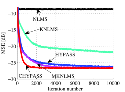
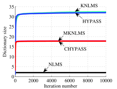
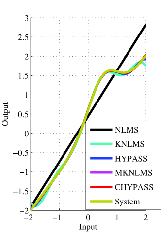
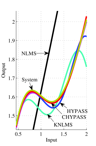
Figure 2: Results for Experiment A1: the linear-Gaussian case.

V-A Toy Models

V-A1 Experiment A1 - Linear Plus Gaussian Case

We consider the following linear-Gaussian model: $\psi(u):=u+\exp\left(-\dfrac{(u-0.5)^{2}}{2\times 0.5^{2}}\right)$ for $u\in\mathcal{U}:=(-2,2)\subset{\mathbb{R}}$ (i.e., $L=1$). We compare the performance of the proposed multikernel adaptive filtering algorithm (CHYPASS) with its alternative (MKNLMS) as well as KNLMS and HYPASS. For fairness, we adopt the same novelty criterion as described in Section III-A, which is basically Platt’s criterion [36], for KNLMS and HYPASS in all experiments. For the multikernel adaptive filtering algorithms, we employ the linear kernel $\kappa_{1}:=w_{1}\kappa_{\rm L}$ for $c:=1$ and a Gaussian kernel $\kappa_{2}:=w_{2}\kappa_{{\rm G},\sigma}$ for $\sigma:=0.5$ (i.e., $Q=2$); the weight is chosen as $w_{1}=w_{2}=0.5$ ($w_{1}+w_{2}=1$). An input sequence $(u_{n})_{n\in{\mathbb{N}}}\subset\mathcal{U}$ is randomly drawn from the uniform distribution over the input space $\mathcal{U}$. The output of the unknown system is corrupted by an additive white Gaussian noise; the observed data is given by $d_{n}:=\psi(u_{n})+v_{n}$ with the Gaussian noise $v_{n}\sim\mathcal{N}(0,2.0\times 10^{-3})$, $n\in{\mathbb{N}}$. We test 300 independent trials and compute the mean squared error (MSE) and the mean dictionary size by averaging the values of $(d_{n}-\varphi_{n}(u_{n}))^{2}$ and $r_{n}:=r_{1,n}+r_{2,n}$, respectively, over the 300 trials at each iteration $n\in{\mathbb{N}}$. The parameters and complexities for each algorithm are summarized in Table II.

Fig. 2 shows (a) the MSE learning curves, (b) the evolutions of the dictionary size, and (c) an instance of the final estimate of each algorithm as well as the system $\psi$ to be estimated. For reference, the results of NLMS (the special case of CHYPASS with $Q=1$, $\kappa_{1}:=\kappa_{\rm L}$ for $c=1$) are included. The mean dictionary size was: KNLMS 31.9, HYPASS 31.6, MKNLMS 17.8, and CHYPASS 17.7. It is seen that both CHYPASS and MKNLMS outperform their single-kernel counterparts with lower complexity. This is due to the simultaneous use of linear and Gaussian kernels under the multikernel adaptive filtering framework. In the left panel of Fig. 2(c), it is seen that all the nonlinear algorithms can estimate $\psi$ well globally. The right panel shows the local behaviors in the specific range $[0.5,2.0]$ of the input space. One can see that the multikernel algorithms better estimate $\psi$ than the single-kernel ones.

V-A2 Experiment A2 - Sinusoid Plus Gaussian Case

We consider the following model which has a low-frequency component (sinusoid) and a high-frequency component (Gaussian): $\psi(u):=\sin\left(\dfrac{\pi}{3}u\right)-\exp\left(-\dfrac{(u-0.5)^{2}}{2\times 0.1^{2}}\right)$ for $u\in\mathcal{U}:=(-2,2)\subset{\mathbb{R}}$ (i.e., $L=1$). We compare CHYPASS and MKNLMS with KNLMS and HYPASS. For the multikernel adaptive filtering algorithms, we employ two Gaussian kernels $\kappa_{1}:=w_{1}\kappa_{{\rm G},\sigma_{1}}$ and $\kappa_{2}:=w_{2}\kappa_{{\rm G},\sigma_{2}}$ for $w_{2}:=0.1$, $w_{1}:=1-w_{2}$, $\sigma_{1}:=1.0$, and $\sigma_{2}:=0.02$ (i.e., $Q=2$). The input and observed data sequences are generated in a way similar to the previous experiment with the noise variance $1.0\times 10^{-3}$. The parameters and complexities for each algorithm are summarized in Table III.

Fig. 3 depicts the results. In Fig. 3(b), the curves labeled as CHYPASS-r1 and MKNLMS-r1 show the evolution of $r_{1,n}$ for each algorithm. The mean dictionary size was: KNLMS 205.0, HYPASS 205.8, MKNLMS 147.6, and CHYPASS 149.3. As in the results of Experiment A1, CHYPASS and MKNLMS outperform their single-kernel counterparts with lower complexity. It is also seen that CHYPASS significantly outperforms MKNLMS. This is because the autocorrelation matrix of the kernelized input vector ${\boldsymbol{k}}_{n}$ has a large eigenvalue spread, whereas the condition number is improved in CHYPASS by using another metric (cf. [40]). Fig. 3(c) shows that the multikernel algorithms better estimate $\psi$ around the edge.

V-A3 Experiment A3 - Partially Linear Case

We consider the following nonlinear dynamic system which has a partially linear structure [30]: $d_{n}:=0.5d_{n-1}+0.2x_{n}+0.3\sin(d_{n-1}x_{n})+v_{n}$, $n\in{\mathbb{N}}$. Here, $x_{n}\sim\mathcal{N}(0,1)$ is the excitation signal and $v_{n}\sim\mathcal{N}(0,1.0\times 10^{-2})$ is the noise. Each datum $d_{n}$ is a function of $u_{n}$ and $d_{n-1}$ and is therefore predicted with ${\boldsymbol{u}}_{n}:=[u_{n},d_{n-1}]^{\sf T}$ (i.e., $L=2$). We employ the linear kernel $\kappa_{1}:=w_{1}\kappa_{\rm L}$ for $c:=1$ and a Gaussian kernel $\kappa_{2}:=w_{2}\kappa_{{\rm G},\sigma}$ for $\sigma:=0.5$ (i.e., $Q=2$). The parameters and complexities for each algorithm are summarized in Table IV. Fig. 4 depicts the results. The mean dictionary size was: KNLMS 181.9, HYPASS 180.0, MKNLMS 104.8, and CHYPASS 104.7. It is consistently observed that CHYPASS and MKNLMS outperform their single-kernel counterparts with lower complexity.

V-B Real Data: Time Series Prediction

V-B1 Experiment B1 - Laser Signal

We use the chaotic laser time series from the Santa Fe time series competition [57] (cf. [2]). The dataset contains 1,000 samples and we use it twice for learning. The maximum value of the data is normalized to one and is then corrupted by noise $v_{n}\sim\mathcal{N}(0,1.0\times 10^{-2})$. We predict each datum $d_{n}$ with a collection of past data ${\boldsymbol{u}}_{n}:=[d_{n-1},d_{n-2}\cdots,d_{n-L+1}]^{\sf T}\in{\mathbb{R}}^{L}$, $n\in{\mathbb{N}}$, for $L=10$. We test two cases of CHYPASS: the linear-Gaussian case (referred to as CHYPASS-LG) and the two-Gaussian case (referred to as CHYPASS-GG). The parameters and complexities for each algorithm are summarized in Table V. Note that the Gaussian kernel is normalized as in (9). In the present case, $(\sqrt{2\pi}\sigma_{1})^{L}\approx 0.98\times 10^{4}$ and $(\sqrt{2\pi}\sigma_{2})^{L}\approx 1.0\times 10^{-3}$. The unbalance due to the use of large $L$ makes the scale of the autocorrelation matrix of ${\boldsymbol{k}}_{2,n}$ be much greater than that of ${\boldsymbol{k}}_{1,n}$ both for CHYPASS and MKNLMS. This causes extremely slow convergence in terms of those coefficients associated with $\kappa_{1}$ and, as a result, the performance of the algorithms becomes almost the same as obtained by the sole use of $\kappa_{2}$. To emphasize the effect of $\kappa_{1}$, a very small value is allocated to $w_{2}$ so that $w_{1}:=1-w_{2}\approx 1.0$. Fig. 5 depicts the results. The mean dictionary size was: HYPASS 62.2, CHYPASS-LG 49.4, and CHYPASS-GG 43.9. It is seen that CHYPASS outperforms HYPASS with lower complexity.

TABLE III: Parameter settings and complexities for Experiment A2.

	parameter		complexity
NLMS	$\lambda_{n}=0.1$		$5$
KNLMS	$\lambda_{n}=0.1$	$\delta=0.8$	$1232$
HYPASS	$\sigma=\sigma_{2}=0.02$	$\delta=0.8$, $s_{n}=1$	$829$
MKNLMS	$\varepsilon=0.01$	$\sigma_{1}=1.0$, $\delta_{1}=0.92$	$897$
(Two-Gaussian)		$\delta=0.6$, $w_{2}=0.1$
CHYPASS		$\sigma_{1}=1.0$, $\delta_{1}=0.92$	$609$
(Two-Gaussian)		$\delta=0.65$, $w_{2}=0.1$
		$s_{n}=1$

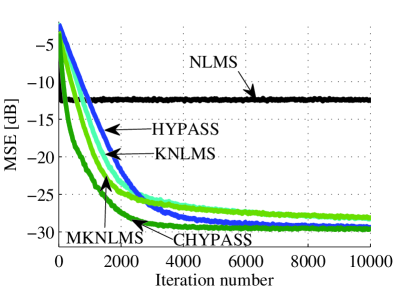
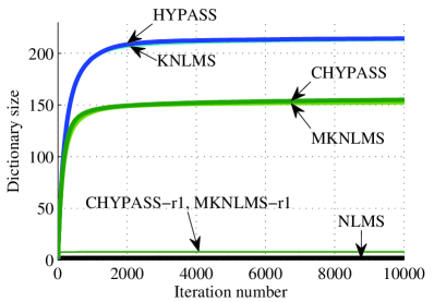
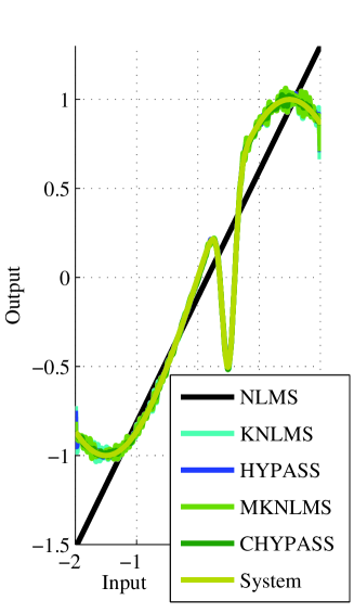
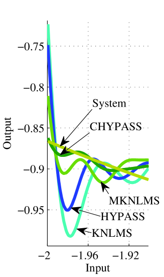
Figure 3: Results for Experiment A2: the sinusoid-Gaussian case.

V-B2 Experiment B2 - CO2 Emission Data

We use a real data of the carbon dioxide emissions from energy consumption in the industrial sector during Jan. 1973 to Jun. 2013, available at the Data Market website (http://datamarket.com/). The dataset contains 486 samples and we use it repeatedly for learning. As in Section V-B1, the maximum value of the data is normalized to one and is then corrupted by noise $v_{n}\sim\mathcal{N}(0,1.0\times 10^{-2})$. Each datum $d_{n}$ is predicted with ${\boldsymbol{u}}_{n}:=[d_{n-1},d_{n-2}\cdots,d_{n-L+1}]^{\sf T}\in{\mathbb{R}}^{L}$, $n\in{\mathbb{N}}$, for $L=20$. We test CHYPASS with two-Gaussian kernels and compare its performance with that of HYPASS. The parameters and complexities for each algorithm are summarized in Table VI. Due to the same idea as in Section V-B1, the weight is designed as $w_{2}:=(\sqrt{2\pi}\sigma_{2})^{L}/(\sqrt{2\pi}\sigma_{1})^{L}\approx 3.5\times 10^{-11}$ and $w_{1}:=1-w_{2}\approx 1.0$. Fig. 6 depicts the results. The mean dictionary size was: HYPASS 268.2, and CHYPASS 191.4. It is seen that CHYPASS significantly outperforms HYPASS, particularly in the initial phase, with lower complexity.

TABLE IV: Parameter settings and complexities for Experiment A3.

	parameter		complexity
NLMS	$\lambda_{n}=0.1$		8
KNLMS	$\lambda_{n}=0.1$	$\delta=0.95$	1275
HYPASS	$\sigma=0.5$	$\delta=0.95$, $s_{n}=1$	906
MKNLMS	$\varepsilon=0.05$	$\delta=0.9$, $w_{1}=0.2$	729
(Linear-Gaussian)
CHYPASS		$\delta=0.9$, $w_{1}=0.1$	524
(Linear-Gaussian)		$s_{n}=1$

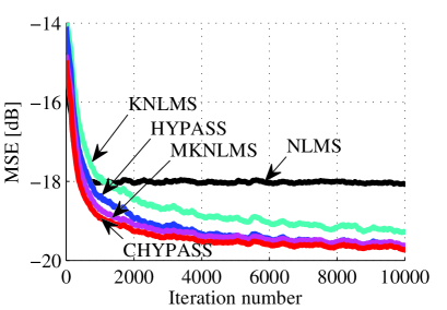
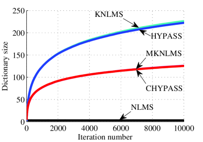
Figure 4: Results for Experiment A3: the partially linear case.

V-C Wrap-up

We finally wrap up this experimental section by reviewing the results from three aspects.

V-C1 Multikernel and Single-kernel Approaches

Comparing the CHYPASS and MKNLMS algorithms with their respective single-kernel counterparts, we can see that the multikernel approach exhibit better MSE performances with smaller dictionary sizes. This indicates that the use of multiple kernels would allow compact representations of unknown systems as mentioned in Section IV-E3.

V-C2 Functional and Parameter-space Approaches

It can be observed that the functional approaches (CHYPASS and HYPASS) outperform the parameter-space approaches (MKNLMS and KNLMS). This would be due to the decorrelation effect inherent in the functional approach according to our experimental studies of HYPASS and CHYPASS. To be specific, we have empirically found that the multiplication of the inverse of the kernel matrix (see Lemma 1) decorrelates the kernelized input vector, yielding the improvements of convergence behaviors.

V-C3 Efficacy of the Selective Updating Strategy

In all the experiments, the size $s_{n}$ of selected subsets is chosen so that any further increase of $s_{n}$ does not improve the performance significantly. In other words, each functional approach for $s_{n}\leq 5$ achieves the best possible performance that is realized by its exact version (i.e., $s_{n}=r_{n}$) which is computationally expensive as explained in Section IV-E. This clearly shows the efficacy of the selective updating strategy.

TABLE V: Parameter settings and complexities for Experiment B1.

	parameter		complexity
HYPASS	$\lambda_{n}=0.1$	$\delta=0.4$, $s_{n}=5$	971
CHYPASS	$\sigma=\sigma_{2}=0.2$	$\delta=0.2$, $s_{n}=5$	698
(Linear-Gaussian)	$\varepsilon=0.05$	$w_{2}=1.0\times 10^{-3}$
CHYPASS		$\sigma_{1}=1$, $\delta_{1}=0.6$	900
(Two-Gaussian)		$\delta=0.2$, $s_{n}=5$
		$w_{2}=1.0\times 10^{-5}$

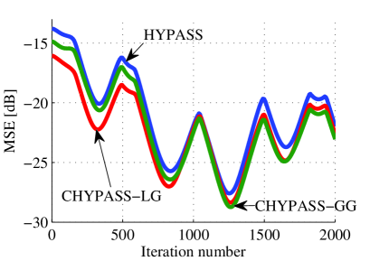
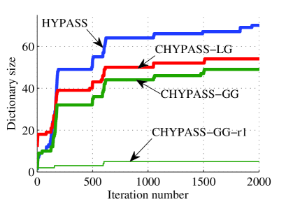
Figure 5: Results for Experiment B1: the laser signal.

TABLE VI: Parameter settings and complexities for Experiment B2.

	parameter		complexity
HYPASS	$\lambda_{n}=0.1$	$s_{n}=5$	6331
CHYPASS	$\sigma=\sigma_{2}=0.3$	$\sigma_{1}=1$, $\delta_{1}=0.95$	4731
(Two-Gaussian)	$\delta=0.95$	$s_{n}=5$
	$\varepsilon=0.01$	$w_{2}=3.5\times 10^{-11}$

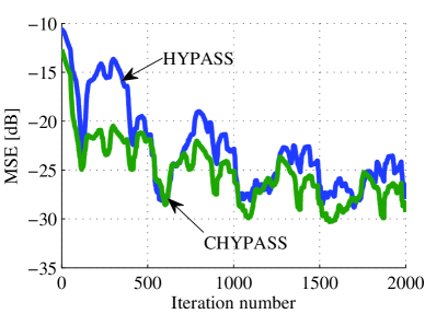
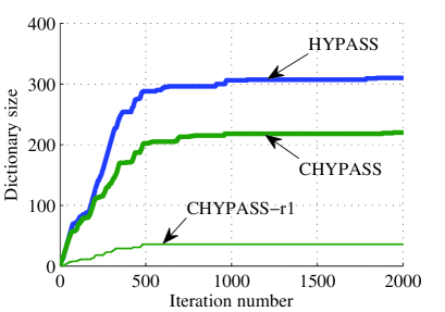
Figure 6: Results for Experiment B2: the CO2 emission data.

VI Concluding Remarks

We proposed the CHYPASS algorithm for the task of estimating/tracking nonlinear functions which contain multiple components. The proposed algorithm is based on iterative orthogonal projections in the Cartesian product of multiple RKHSs. The proposed algorithm was derived by reformulating the HYPASS algorithm in the product space. In the particular case (including the linear-Gaussian case), the proposed algorithm can also be regarded as operating iterative projections in the ‘sum’ space of the RKHSs. The numerical examples with three toy models and two real data demonstrated that the simultaneous use of multiple kernels led to a compact representation of the nonlinear functions and yielded better performance than the single-kernel algorithms.

The two streams of multikernel adaptive filtering and HYPASS have met and united. The key idea for the union was presented in the simplest possible way by focusing on the NLMS-type algorithm. It is our future work of significant interest to extend CHYPASS to a more sophisticated one such as a $\Phi$-PASS type algorithm; $\Phi$-PASS is based on parallel projection and thus enjoys better convergence properties than HYPASS [37, 35]. Further investigations are definitely required to verify the practical value of the proposed Cartesian-product projection approach in real-world applications. It is also our important future issue to verify the decorrelation effect mentioned in Section V-C2 from the theoretical and/or experimental viewpoints.

Appendix A Kernel Ridge Regression in Sum Space

We present a basic theorem for the batch case.

Theorem A.1 (Kernel Ridge Regression in Sum Space)

Given a set of finite samples $\{({\boldsymbol{u}}_{j},d_{j})\}_{j=1}^{r}$, define a regularized risk functional $R_{c}(f)$ of $f\in{\mathcal{H}}^{+}$ as

$$R_{c}(f):=\frac{1}{r}\sum_{j=1}^{r}\left(f({\boldsymbol{u}}_{j})-d_{j}\right)^{2}+\eta\left\|f\right\|_{{\mathcal{H}}^{+}}^{2},~{}~{}~{}\eta>0.$$ (A.1)

Then, the minimizer $f^{*}:=\operatornamewithlimits{argmin}_{f\in{\mathcal{H}}^{+}}R_{c}(f)$ is given by $f^{*}=\sum_{j=1}^{r}\alpha_{j}\kappa(\cdot,{\boldsymbol{u}}_{j})$ with $[\alpha_{1},\alpha_{2},\cdots,\alpha_{r}]^{\sf T}:=({\boldsymbol{K}}+\eta r{\boldsymbol{I}})^{-1}[d_{1},d_{2},\cdots,d_{r}]^{\sf T}$, where ${\boldsymbol{K}}\in{\mathbb{R}}^{r\times r}$ is the kernel matrix whose $(i,j)$ entry is $\kappa({\boldsymbol{u}}_{i},{\boldsymbol{u}}_{j})$.

The result in [31, Theorem 1] can be reproduced by applying Theorem A.1 with a weighted norm and its associated kernel given in Corollary 1.

References

- [1] J. Kivinen, A. J. Smola, and R. C. Williamson, “Online learning with kernels,” IEEE Trans. Signal Process., vol. 52, no. 8, pp. 2165–2176, Aug. 2004.
- [2] Y. Engel, S. Mannor, and R. Meir, “The kernel recursive least-squares algorithm,” IEEE Trans. Signal Process., vol. 52, no. 8, pp. 2275–2285, Aug. 2004.
- [3] A. V. Malipatil, Y.-F. Huang, S. Andra, and K. Bennett, “Kernelized set-membership approach to nonlinear adaptive filtering,” in Proc. IEEE ICASSP, 2005, pp. 149–152.
- [4] W. Liu and J. Príncipe, “Kernel affine projection algorithms,” EURASIP J. Adv. Signal Process., vol. 2008, pp. 1–12, 2008, article ID 784292.
- [5] K. Slavakis, S. Theodoridis, and I. Yamada, “Online kernel-based classification using adaptive projection algorithms,” IEEE Trans. Signal Process., vol. 56, no. 7, pp. 2781–2796, July 2008.
- [6] ——, “Adaptive constrained learning in reproducing kernel Hilbert spaces: the robust beamforming case,” IEEE Trans. Signal Process., vol. 57, no. 12, pp. 4744–4764, Dec. 2009.
- [7] C. Richard, J. Bermudez, and P. Honeine, “Online prediction of time series data with kernels,” IEEE Trans. Signal Process., vol. 57, no. 3, pp. 1058–1067, Mar. 2009.
- [8] W. Liu, J. Príncipe, and S. Haykin, Kernel Adaptive Filtering. New Jersey: Wiley, 2010.
- [9] S. Theodoridis, K. Slavakis, and I. Yamada, “Adaptive learning in a world of projections: a unifying framework for linear and nonlinear classification and regression tasks,” IEEE Signal Process. Mag., vol. 28, no. 1, pp. 97–123, Jan. 2011.
- [10] S. Van Vaerenbergh, M. Lázaro-Gredilla, and I. Santamaría, “Kernel recursive least-squares tracker for time-varying regression,” IEEE Trans. Neural Networks and Learning Systems, vol. 23, no. 8, pp. 1313–1326, Aug. 2012.
- [11] K. Slavakis, P. Bouboulis, and S. Theodoridis, “Online learning in reproducing kernel Hilbert spaces,” in Academic Press Library in Signal Processing: 1st Edition, Signal Processing Theory and Machine Learning. Elsevier, 2014, vol. 1, pp. 883–987.
- [12] N. Aronszajn, “Theory of reproducing kernels,” Trans. Amer. Math. Soc., vol. 68, no. 3, pp. 337–404, May 1950.
- [13] S. Saitoh, Integral Transforms, Reproducing Kernels and Their Applications, ser. Pitman Research Notes in Mathematics. Addison Wesley Longman, 1997, vol. 369.
- [14] V. N. Vapnik, Statistical Learning Theory. New York: Wiley, 1998.
- [15] K.-R. Müller, S. Mika, G. Rätsch, K. Tsuda, and B. Schölkopf, “An introduction to kernel-based learning algorithms,” IEEE Trans. Neural Networks, vol. 12, no. 2, pp. 181–201, Mar. 2001.
- [16] B. Schölkopf and A. J. Smola, Learning with Kernels. Cambridge, MA: MIT Press, 2001.
- [17] A. Berlinet and C. Thomas-Agnan, Reproducing kernel Hilbert spaces in probability and statistics. Boston: MA: Kluwer Academic, 2004.
- [18] J. Shawe-Taylor and N. Cristianini, Kernel Methods for Pattern Analysis. Cambridge University Press, 2004.
- [19] S. Theodoridis and K. Koutroumbas, Pattern Recognition, 4th ed. New York: Academic, 2008.
- [20] IEEE Signal Processing Magazine, Special Section: Advances in Kernel-based Learning for Signal Processing, July 2013.
- [21] Y. Motai, “Kernel association for classification and prediction: a survey,” IEEE Trans. Neural Networks and Learning Systems, 2014, to appear.
- [22] M. Yukawa, “On use of multiple kernels in adaptive learning —Extended reproducing kernel Hilbert space with Cartesian product,” in Proc. IEICE Signal Processing Symposium, Nov. 2010, pp. 59–64.
- [23] ——, “Nonlinear adaptive filtering techniques with multiple kernels,” in European Signal Processing Conference (EUSIPCO), 2011, pp. 136–140.
- [24] ——, “Multikernel adaptive filtering,” IEEE Trans. Signal Processing, vol. 60, no. 9, pp. 4672–4682, Sept. 2012.
- [25] R. Pokharel, J. Príncipe, and S. Seth, “Mixture kernel least mean square,” in IEEE IJCNN, 2013.
- [26] W. Gao, C. Richard, J.-C. M. Bermudez, and J. Huang, “Convex combinations of kernel adaptive filters,” in IEEE Int. Workshop on MLSP, 2014.
- [27] F. A. Tobar, S.-Y. Kung, and D. P. Mandic, “Multikernel least mean square algorithm,” IEEE Trans. Neural Networks and Learning Systems, vol. 25, no. 2, pp. 265–277, Feb. 2014.
- [28] W. Härdle, H. Liang, and J. Gao, Partially Linear Models. Heidelberg, Germany: Physica-Verlag, 2000.
- [29] M. Espinoza, J. A. K. Suykens, and B. D. Moor, “Kernel based partially linear models and nonlinear identification,” IEEE Trans. Autom. Control, vol. 50, no. 10, pp. 1602–1606, Oct. 2005.
- [30] Y.-L. Xu and D.-R. Chen, “Partially-linear least-squares regularized regression for system identification,” IEEE Trans. Autom. Control, vol. 54, no. 11, pp. 2637–2641, Nov. 2009.
- [31] Y.-L. Xu, D.-R. Chen, H.-X. Li, and L. Liu, “Least square regularized regression in sum space,” IEEE Trans. Neural Networks and Learning Systems, vol. 24, no. 4, pp. 635–646, Apr. 2013.
- [32] M. Yukawa and R. Ishii, “Online model selection and learning by multikernel adaptive filtering,” in Proc. EUSIPCO, 2013.
- [33] ——, “On adaptivity of online model selection method based on multikernel adaptive filtering,” in Proc. APSIPA Annual Summit and Conference, 2013.
- [34] ——, “An efficient kernel adaptive filtering algorithm using hyperplane projection along affine subspace,” in Proc. EUSIPCO, 2012, pp. 2183–2187.
- [35] M. Takizawa and M. Yukawa, “Adaptive nonlinear estimation based on parallel projection along affine subspaces in reproducing kernel Hilbert space”,” IEEE Trans. Signal Processing, 2014, submitted.
- [36] J. Platt, “A resource-allocating network for function interpolation,” Neural Computation, vol. 3, no. 2, pp. 213–225, 1991.
- [37] M. Takizawa and M. Yukawa, “An efficient data-reusing kernel adaptive filtering algorithm based on parallel hyperslab projection along affine subspaces,” in Proc. IEEE ICASSP, 2013, pp. 3557–3561.
- [38] T. J. Dodd, V. Kadirkamanathan, and R. F. Harrison, “Function estimation in Hilbert space using sequential projections,” in IFAC Conf. Intell. Control Syst. Signal Process., 2003, pp. 113–118.
- [39] B. Chen, S. Zhao, P. Zhu, and J. C. Príncipe, “Quantized kernel least mean square algorithm,” IEEE Trans. Neural Networks and Learning Systems, vol. 23, no. 1, pp. 22–32, Jan. 2012.
- [40] M. Takizawa and M. Yukawa, “An efficient sparse kernel adaptive filtering algorithm based on isomorphism between functional subspace and Euclidean space,” in Proc. IEEE ICASSP, 2014, pp. 4541–4545.
- [41] R. Vert and J. P. Vert, “Consistency and convergence rates of one-class SVMs and related algorithms,” J. Mach. Learn. Res., vol. 5, pp. 817–854, 2006.
- [42] I. Steinwart, D. Hush, and C. Scovel, “An explicit description of the reproducing kernel Hilbert spaces of Gaussian RBF kernels,” IEEE Trans. Inform. Theory, vol. 52, no. 10, pp. 4635–4643, Oct. 2006.
- [43] A. Tanaka, H. Imai, M. Kudo, and M. Miyakoshi, “Theoretical analyses on a class of nested RKHS’s,” in Proc. IEEE ICASSP, 2011, pp. 2072–2075.
- [44] H. Q. Minh, “Some properties of Gaussian reproducing kernel Hilbert spaces and their implications for function approximation and learning theory,” Constr. Approx., vol. 32, no. 2, pp. 307–338, Oct. 2010.
- [45] D. G. Luenberger, Optimization by Vector Space Methods. New York: Wiley, 1969.
- [46] J. M. Gil-Cacho, M. Signoretto, T. van Waterschoot, M. Moonen, and S. H. Jensen, “Nonlinear acoustic echo cancellation based on a sliding-window leaky kernel affine projection algorithm,” IEEE Trans. Audio, Speech and Language Processing, vol. 21, no. 9, pp. 1867–1878, Sept. 2013.
- [47] M. Yukawa, “Online learning based on iterative projections in sum space of linear and Gaussian reproducing kernel Hilbert spaces,” submitted to IEEE ICASSP 2015.
- [48] B. Chen, S. Zhao, S. Seth, and J. C. Príncipe, “Online efficient learning with quantized KLMS and regularization,” in Int. Joint Conf. Neural Netw., 2012.
- [49] W. Gao, J. Chen, C. Richard, and J. Huang, “Online dictionary learning for kernel LMS,” IEEE Trans. Signal Processing, vol. 62, no. 11, pp. 2765–2777, Jun. 2014.
- [50] J. Nagumo and J. Noda, “A learning method for system identification,” IEEE Trans. Autom. Control, vol. 12, no. 3, pp. 282–287, 1967.
- [51] A. E. Albert and L. S. Gardner Jr., Stochastic Approximation and Nonlinear Regression. Cambridge MA: MIT Press, 1967.
- [52] I. Yamada and N. Ogura, “Adaptive projected subgradient method for asymptotic minimization of sequence of nonnegative convex functions,” Numer. Funct. Anal. Optim., vol. 25, no. 7&8, pp. 593–617, 2004.
- [53] M. Yukawa and I. Yamada, “A unified view of adaptive variable-metric projection algorithms,” EURASIP J. Advances in Signal Processing, vol. 2009, Article ID 589260, 13 pages, 2009.
- [54] M. Yukawa, “Cartesian multikernel adaptive filtering,” IEICE, Tech. Rep., Jan. 2014, SIP2013-104, vol. 113, no. 385, pp. 113–116.
- [55] T. Ishida and T. Tanaka, “Multikernel adaptive filters with multiple dictionaries and regularization,” in Proc. APSIPA-ASC, 2013.
- [56] R. A. Horn and C. R. Johnson, Matrix Analysis. New York: Cambridge University Press, 1985.
- [57] A. S. Weigend and N. A. Gershenfeld, Eds., Time Series Prediction: Forecasting the Future and Understanding the Past. MA: Addison-Wesley: Reading, 1994.