Optimality of doubly reflected LÉVY processes in singular control

Abstract.

We consider a class of two-sided singular control problems. A controller either increases or decreases a given spectrally negative Lévy process so as to minimize the total costs comprising of the running and controlling costs where the latter is proportional to the size of control. We provide a sufficient condition for the optimality of a double barrier strategy, and in particular show that it holds when the running cost function is convex. Using the fluctuation theory of doubly reflected Lévy processes, we express concisely the optimal strategy as well as the value function using the scale function. Numerical examples are provided to confirm the analytical results.
AMS 2010 Subject Classifications: 60G51, 93E20, 49J40
Key words: singular control; doubly reflected Lévy processes; fluctuation theory; scale functions

1. Introduction

We consider the problem of optimally modifying a stochastic process by means of singular control. An admissible strategy is two-sided and the process can be increased or decreased. The objective is to minimize the expected total costs comprising of the running and controlling costs; the former is modeled as some given function $f$ of the controlled process that is accumulated over time, and the latter is proportional to the size of control. The problem of singular control arises in various contexts. For its applications, we refer the reader to, e.g., [14, 15] for inventory management, [19] for cash balance management, [5, 24] for monotone follower problems and [1, 6, 20, 30, 32, 36] for finance and insurance.

This paper studies a spectrally negative Lévy model where the underlying process, in the absence of control, follows a general Lévy process with only negative jumps. We pursue a sufficient condition on the running cost function $f$ such that a strategy of double barrier type is optimal and the value function is obtained semi-explicitly. This generalizes the classical Brownian motion model [21] and complements the results on the continuous diffusion model as in [31].

Motivated by the recent research of spectrally negative Lévy processes and their applications, we take advantage of their fluctuation theory as in [10, 28]. These techniques are used extensively in stochastic control problems in the last decade. Exemplifying examples include de Finetti’s dividend problem as in [1, 6, 30], where a single barrier strategy is shown to be optimal under certain conditions. In these papers, the so-called scale function is commonly used to express the net present value of the barrier strategy. Thanks to its analytical properties such as continuity/smoothness (see, e.g., [23, 28]), the selection of the candidate barrier level and the verification of optimality can be carried out efficiently. While a part of the verification is still problem-dependent and is often a difficult task, these methods allow one to solve for this wide class of Lévy processes without specializing on a particular type, whether or not the process is of infinite activity/variation.

This paper considers a variant of the above mentioned papers where the control is allowed to be two-sided. Our objective is to show the optimality of a double barrier strategy where the resulting controlled process becomes a doubly reflected Lévy process of [1, 34]. Existing research on the optimality of doubly reflected Lévy processes includes the dividend problem with capital injection as in [1, 6]. Other related problems where two threshold levels characterize the optimal strategy include stochastic games [4, 3, 16, 22] and impulse control [7, 38].

In this paper, we take the following steps to achieve our goal:

1. We first write via the scale function the expected net present value corresponding to the double barrier strategy; this is a direct application of the results in [1, 34].

2. This is followed by the selection of the two barriers. The upper barrier is chosen so that the resulting candidate value function becomes twice differentiable at the barrier; the lower barrier is chosen so that it is continously (resp. twice) differentiable when the process is of bounded (resp. unbounded variation).

3. We then analyze the existence of such a pair that satisfy the two conditions simultaneously. We show that either such a pair exist, or otherwise a single barrier strategy (with the upper barrier set to infinity) is optimal.

4. In order to verify the optimality of the strategy defined in the previous steps, we study the verification lemma and identify some additional conditions that are sufficient for the optimality. Moreover, we show that it is satisfied whenever the running cost function $f$ is convex.

As in the above mentioned papers, we use the special known properties of the scale function to solve the problem. In particular, the steps taken here are similar to those used in [22], where two parameters are shown to characterize the optimal strategies in the two-person game they considered. The main novelty and challenge here are that we solve the problem without specifying the form of the running cost function $f$ and derive a most general condition on $f$ that is sufficient for the optimality of a doubly reflected Lévy process.

In addition to the above, we give examples with (piecewise) quadratic and linear cases for $f$, which have been used in, e.g., [2, 13, 37]. We shall see in particular that in the linear case the upper boundary can become infinity (or equivalently a single barrier strategy is optimal), whereas it does not occur in the quadratic case. In order to confirm the obtained analytical results, we give numerical examples where the underlying process is a spectrally negative Lévy process in the $\beta$-family of Kuznetsov [25].

The rest of the paper is organized as follows. Section 2 gives a mathematical model of the problem and a brief review on the spectrally negative Lévy process and the scale function. Section 3 expresses via the scale function the expected net present value under the double barrier strategy. The candidate barrier levels are then selected by using the smoothness conditions at the barriers, and the existence of such a pair is shown. In Section 4, we study the verification lemma for this problem and analyze what additional conditions are required for the candidate value function to be optimal. Section 5 obtains a more concrete sufficient condition and in particular shows that it is satisfied when $f$ is convex. In Section 6, we give examples with piecewise quadratic and linear cases. We conclude the paper with numerical examples in Section 7.

Throughout the paper, $x+$ and $x-$ are used to indicate the right and left hand limits, respectively. The superscripts $x^{+}:=\max(x,0)$, $f^{+}(x):=\max(f(x),0)$, $x^{-}:=\max(-x,0)$ and $f^{-}(x):=\max(-f(x),0)$ are used to indicate positive and negative parts. Monotonicity is understood in the strict sense; for the weak sense “nondecreasing” and “nonincreasing” are used. The convexity (unless otherwise stated) is in the weak sense.

2. Mathematical Formulation

Let $(\Omega,\mathcal{F},\mathbb{P})$ be a probability space hosting a spectrally negative Lévy process $X=\left\{X_{t};t\geq 0\right\}$ whose Laplace exponent is given by

(2.1) $$\psi(s):=\log\mathbb{E}\left[e^{sX_{1}}\right]=cs+\frac{1}{2}\sigma^{2}s^{2}+\int_{(-\infty,0)}(e^{sz}-1-sz1_{\{-1<z<0\}})\nu({\rm d}z),\quad s\geq 0,$$

where $\nu$ is a Lévy measure with the support $(-\infty,0)$ that satisfies the integrability condition $\int_{(-\infty,0)}(1\wedge z^{2})\nu({\rm d}z)<\infty$. It has paths of bounded variation if and only if $\sigma=0$ and $\int_{(-1,0)}|z|\,\nu({\rm d}z)<\infty$; in this case, we write (2.1) as

$$\psi(s)=\delta s+\int_{(-\infty,0)}(e^{sz}-1)\nu({\rm d}z),\quad s\geq 0,$$

with $\delta:=c-\int_{(-1,0)}z\,\nu({\rm d}z)$. We exclude the case in which $X$ is the negative of a subordinator (i.e., $X$ has monotone paths a.s.). This assumption implies that $\delta>0$ when $X$ is of bounded variation. Let $\mathbb{P}_{x}$ be the conditional probability under which $X_{0}=x$ (also let $\mathbb{P}\equiv\mathbb{P}_{0}$), and let $\mathbb{F}:=\left\{\mathcal{F}_{t},t\geq 0\right\}$ be the filtration generated by $X$.

An admissible strategy $\pi:=\left\{(U_{t}^{\pi},D_{t}^{\pi});t\geq 0\right\}$ is given by a pair of nondecreasing, right-continuous and $\mathbb{F}$-adapted processes such that $U^{\pi}_{0-}=D^{\pi}_{0-}=0$ and, as is assumed in [21],

(2.2) $$\mathbb{E}_{x}\Big{[}\int_{[0,\infty)}e^{-qt}({\rm d}U^{\pi}_{t}+{\rm d}D^{\pi}_{t})\Big{]}<\infty,\quad x\in\mathbb{R}.$$

Let $\Pi$ be the set of all admissible strategies and the discount $q$ is assumed to be a strictly positive constant.

With the controlled process $Y_{t}^{\pi}:=X_{t}+U_{t}^{\pi}-D_{t}^{\pi}$, $t\geq 0$, the problem is to compute the total expected costs:

$$v^{\pi}(x):=\mathbb{E}_{x}\Big{[}\int_{0}^{\infty}e^{-qt}f(Y_{t}^{\pi}){\rm d}t+\int_{[0,\infty)}e^{-qt}\left(C_{U}{\rm d}U^{\pi}_{t}+C_{D}{\rm d}D^{\pi}_{t}\right)\Big{]},\quad x\in\mathbb{R},$$

for some running cost function $f$ satisfying the conditions specified below and fixed constants $C_{U},C_{D}\in\mathbb{R}$ such that

(2.3) $$C_{U}+C_{D}>0,$$

and to obtain an admissible strategy over $\Pi$ that minimizes it, if such a strategy exists. The inequality (2.3) is commonly assumed in the literature (see, e.g., [21, 31]); this implies that it is suboptimal to activate $U_{t}^{\pi}$ and $D_{t}^{\pi}$ simultaneously. Hence, we can safely assume that the supports of the Stieltjes measures ${\rm d}U_{t}^{\pi}(\omega)$ and ${\rm d}D_{t}^{\pi}(\omega)$ do not overlap for a.e. $\omega\in\Omega$.

Regarding the running cost function $f$, we assume the same assumptions as in [8, 9, 38]; this is a crucial condition when dealing with a process with negative jumps.

Assumption 2.1.

We assume that $f:\mathbb{R}\rightarrow\mathbb{R}$ satisfies the following.

1. $f$ is continuous and is a piecewise continuously differentiable function and grows (or decreases) at most polynomially (in the sense defined by Beyer et al. [11]).

2. There exists a number $\overline{a}\in\mathbb{R}$ such that the function

   (2.4) $$\tilde{f}(x) :=f(x)+C_{U}qx,\quad x\in\mathbb{R},$$

   is increasing on $(\overline{a},\infty)$ and is decreasing and convex on $(-\infty,\overline{a})$.

3. There exist a $c_{0}>0$ and an $x_{0}\geq\overline{a}$ such that $\tilde{f}^{\prime}(x)\geq c_{0}$ for $x\geq x_{0}$.

For the problem to make sense, we assume that the Lévy process $X$ has a finite moment.

Assumption 2.2.

We assume that $\mathbb{E}[X_{1}]=\psi^{\prime}(0+)\in(-\infty,\infty)$.

2.1. Scale functions

Fix $q>0$. For any spectrally negative Lévy process, there exists a function called the $q$-scale function

$$W^{(q)}:\mathbb{R}\rightarrow[0,\infty),$$

which is zero on $(-\infty,0)$, continuous and increasing on $[0,\infty)$, and is characterized by the Laplace transform:

$$\int_{0}^{\infty}e^{-sx}W^{(q)}(x){\rm d}x=\frac{1}{\psi(s)-q},\qquad s>\Phi(q),$$

where

$$\Phi(q):=\sup\{\lambda\geq 0:\psi(\lambda)=q\}.$$

Here, the Laplace exponent $\psi$ in (2.1) is known to be zero at the origin and strictly convex on $[0,\infty)$; therefore $\Phi(q)$ is well defined and is strictly positive as $q>0$. We also define, for $x\in\mathbb{R}$,

$$\overline{W}^{(q)}(x) :=\int_{0}^{x}W^{(q)}(y){\rm d}y,$$

$$Z^{(q)}(x) :=1+q\overline{W}^{(q)}(x),$$

$$\overline{Z}^{(q)}(x) :=\int_{0}^{x}Z^{(q)}(z){\rm d}z=x+q\int_{0}^{x}\int_{0}^{z}W^{(q)}(w){\rm d}w{\rm d}z.$$

Because $W^{(q)}$ is uniformly zero on the negative half line, we have

(2.5) $$Z^{(q)}(x)=1\quad\textrm{and}\quad\overline{Z}^{(q)}(x)=x,\quad x\leq 0.$$

Let us define the first down- and up-crossing times, respectively, of $X$ by

$$\tau_{b}^{-}:=\inf\left\{t\geq 0:X_{t}<b\right\}\quad\textrm{and}\quad\tau_{b}^{+}:=\inf\left\{t\geq 0:X_{t}>b\right\},\quad b\in\mathbb{R}.$$

Then, for any $b>0$ and $x\leq b$,

(2.6) $$\mathbb{E}_{x}\left[e^{-q\tau_{b}^{+}}1_{\left\{\tau_{b}^{+}<\tau_{0}^{-}\right\}}\right]=\frac{W^{(q)}(x)}{W^{(q)}(b)}\quad\textrm{and}\quad\mathbb{E}_{x}\left[e^{-q\tau_{0}^{-}}1_{\left\{\tau_{b}^{+}>\tau_{0}^{-}\right\}}\right]=Z^{(q)}(x)-Z^{(q)}(b)\frac{W^{(q)}(x)}{W^{(q)}(b)}.$$

By taking limits on the latter,

$$\mathbb{E}_{x}\left[e^{-q\tau_{0}^{-}}\right] =Z^{(q)}(x)-\frac{q}{\Phi(q)}W^{(q)}(x),\quad x\in\mathbb{R}.$$

Fix $\lambda\geq 0$ and define $\psi_{\lambda}(\cdot)$ as the Laplace exponent of $X$ under $\mathbb{P}^{\lambda}$ with the change of measure

$$\left.\frac{{\rm d}\mathbb{P}^{\lambda}}{{\rm d}\mathbb{P}}\right|_{\mathcal{F}_{t}}=\exp(\lambda X_{t}-\psi(\lambda)t),\quad t\geq 0;$$

see page 213 of [28]. Suppose $W_{\lambda}^{(q)}$ and $Z_{\lambda}^{(q)}$ are the scale functions associated with $X$ under $\mathbb{P}^{\lambda}$ (or equivalently with $\psi_{\lambda}(\cdot)$). Then, by Lemma 8.4 of [28], $W_{\lambda}^{(q-\psi(\lambda))}(x)=e^{-\lambda x}W^{(q)}(x)$, $x\in\mathbb{R}$, which is well defined even for $q\leq\psi(\lambda)$ by Lemmas 8.3 and 8.5 of [28]. In particular, we define

(2.7) $$W_{\Phi(q)}(x):=W_{\Phi(q)}^{(0)}(x)=e^{-\Phi(q)x}W^{(q)}(x),\quad x\in\mathbb{R},$$

which is known to be an increasing function and, as in Lemma 3.3 of [27],

(2.8) $$W_{\Phi(q)}(x)\nearrow\psi^{\prime}(\Phi(q))^{-1}\quad\textrm{as }x\rightarrow\infty.$$

Remark 2.1.

1. If $X$ is of unbounded variation or the Lévy measure is atomless, it is known that $W^{(q)}$ is $C^{1}(\mathbb{R}\backslash\{0\})$; see, e.g., [12]. Hence,

   1. $Z^{(q)}$ is $C^{1}(\mathbb{R}\backslash\{0\})$ and $C^{0}(\mathbb{R})$ for the bounded variation case, while it is $C^{2}(\mathbb{R}\backslash\{0\})$ and $C^{1}(\mathbb{R})$ for the unbounded variation case, and

   2. $\overline{Z}^{(q)}$ is $C^{2}(\mathbb{R}\backslash\{0\})$ and $C^{1}(\mathbb{R})$ for the bounded variation case, while it is $C^{3}(\mathbb{R}\backslash\{0\})$ and $C^{2}(\mathbb{R})$ for the unbounded variation case.

2. Regarding the asymptotic behavior near zero, as in Lemmas 4.3 and 4.4 of [29],

   (2.9) $$\begin{split}W^{(q)}(0)&=\left\{\begin{array}[]{ll}0,&\textrm{if $X$ is of unbounded variation,}\\ \frac{1}{\delta},&\textrm{if $X$ is of bounded variation,}\end{array}\right.\\ W^{(q)^{\prime}}(0+)&:=\lim_{x\downarrow 0}W^{(q)^{\prime}}(x)=\left\{\begin{array}[]{ll}\frac{2}{\sigma^{2}},&\textrm{if }\sigma>0,\\ \infty,&\textrm{if }\sigma=0\;\textrm{and}\;\nu(-\infty,0)=\infty,\\ \frac{q+\nu(-\infty,0)}{\delta^{2}},&\textrm{if }\sigma=0\;\textrm{and}\;\nu(-\infty,0)<\infty.\end{array}\right.\end{split}$$

3. As in (8.18) and Lemma 8.2 of [28],

   $$\frac{W^{(q)^{\prime}}(y+)}{W^{(q)}(y)}\leq\frac{W^{(q)^{\prime}}(x+)}{W^{(q)}(x)},\quad y>x>0.$$

   In all cases, $W^{(q)^{\prime}}(x-)\geq W^{(q)^{\prime}}(x+)$ for all $x>0$.

The problem in this paper is a generalization of Section 6 of [38], where $D_{t}^{\pi}$ is restricted to be zero. Its optimal solution is a (single) barrier strategy, which is described immediately below. Define, for any measurable function $h$ and $s\in\mathbb{R}$,

$$\begin{split}\Psi(s;h)&:=\int_{0}^{\infty}e^{-\Phi(q)y}h(y+s){\rm d}y=\int_{s}^{\infty}e^{-\Phi(q)(y-s)}h(y){\rm d}y,\\ \varphi_{s}(x;h)&:=\int_{s}^{x}W^{(q)}(x-y)h(y){\rm d}y,\quad x\in\mathbb{R}.\end{split}$$

Here $\varphi_{s}(x;h)=0$ for any $x\leq s$ because $W^{(q)}$ is uniformly zero on $(-\infty,0)$.

The following, which holds directly from Assumption 2.1, is due to [9]. Here note that $\Psi(\cdot;\tilde{f}^{\prime})$ is equivalent to (4.23) of [9] (times a positive constant). While in [9], they focus on a special class of spectrally negative Lévy processes, the results still hold for a general spectrally negative Lévy process.

Lemma 2.1 (Proposition 5.1 of [9]).

1. There exists a unique number $\underline{a}<\overline{a}$ such that $\Psi(\underline{a};\tilde{f}^{\prime})=0$, $\Psi(x;\tilde{f}^{\prime})<0$ if $x<\underline{a}$ and $\Psi(x;\tilde{f}^{\prime})>0$ if $x>\underline{a}$.

2. $\Psi^{\prime}(x;\tilde{f}^{\prime})>0$ for $x\leq\overline{a}$.

3. $\Psi(x;\tilde{f}^{\prime})\geq c_{0}/\Phi(q)$ for $x\geq x_{0}$.

Namely, while $\overline{a}$ is the unique zero of $\tilde{f}^{\prime}$, $\underline{a}$ is the unique zero of $\Psi(\cdot;\tilde{f}^{\prime})$. We are now ready to state the results of the auxiliary problem.

Theorem 2.1 (Theorem 6.1 of [38]).

Consider a version of the problem that minimizes

$$\tilde{v}^{\pi}(x):=\mathbb{E}_{x}\Big{[}\int_{0}^{\infty}e^{-qt}f(\widetilde{Y}_{t}^{\pi}){\rm d}t+\int_{[0,\infty)}e^{-qt}C_{U}{\rm d}U^{\pi}_{t}\Big{]},\quad x\in\mathbb{R},$$

with the controlled process $\widetilde{Y}_{t}^{\pi}:=X_{t}+U_{t}^{\pi}$, $t\geq 0$ for some fixed constant $C_{U}\in\mathbb{R}$, that satisfies Assumption 2.1.

Then the barrier strategy $U^{\underline{a},\infty}$ defined by

(2.10) $$U^{\underline{a},\infty}_{t}:=\sup_{0\leq t^{\prime}\leq t}({\underline{a}}-X_{t^{\prime}})\vee 0,\quad t\geq 0,$$

is optimal and the value function is

(2.11) $$\begin{split}\inf_{\pi}\tilde{v}^{\pi}(x)=\tilde{v}_{\underline{a}}(x)&:=-C_{U}\left(\overline{Z}^{(q)}(x-\underline{a})+\frac{\psi^{\prime}(0+)}{q}\right)+\frac{f(\underline{a})}{q}Z^{(q)}(x-\underline{a})-\varphi_{\underline{a}}(x;f).\end{split}$$

3. The double barrier strategies

Following Avram et al. [1] and Pistorius [33], we define a doubly reflected Lévy process given by

$$Y_{t}^{a,b}:=X_{t}+U_{t}^{a,b}-D_{t}^{a,b},\quad t\geq 0,\;a<b,$$

which is reflected at two barriers $a$ and $b$ so as to stay on the interval $[a,b]$; see page 165 of [1] for the construction of this process. We let $\pi_{a,b}$ be the corresponding strategy and $v_{a,b}$ the corresponding expected total cost. Our aim is to show that by choosing the values of $(a,b)$ appropriately, the minimization is attained by the strategy $\pi_{a,b}$.

For $b\geq a$, let

(3.1) $$\begin{split}\Gamma(a,b)&:=C_{D}+C_{U}Z^{(q)}(b-a)+f(b)W^{(q)}(0)+\int_{a}^{b}f(y){W^{(q)^{\prime}}(b-y)}{\rm d}y-W^{(q)}(b-a)f(a)\\ &=C_{D}+C_{U}+\varphi_{a}(b;\tilde{f}^{\prime}).\end{split}$$

Also let

$$R^{(q)}(y):=\overline{Z}^{(q)}(y)+\frac{\psi^{\prime}(0+)}{q},\quad y\in\mathbb{R}.$$

Lemma 3.1.

Fix any $a<b$. We have $\pi_{a,b}\in\Pi$. Moreover, for $x\leq b$,

(3.2) $$\begin{split}v_{a,b}(x)&=\frac{\Gamma(a,b)}{qW^{(q)}(b-a)}{Z^{(q)}(x-a)}-C_{U}R^{(q)}(x-a)+\frac{f(a)}{q}Z^{(q)}(x-a)-\varphi_{a}(x;f)\\ &=\frac{\Gamma(a,b)}{qW^{(q)}(b-a)}{Z^{(q)}(x-a)}-C_{U}R^{(q)}(x-a)+\frac{f(a)}{q}-\int_{a}^{x}\overline{W}^{(q)}(x-y)f^{\prime}(y){\rm d}y.\end{split}$$

For $x\geq b$, we have $v_{a,b}(x)=v_{a,b}(b)+C_{D}(x-b)$.

Proof.

As in Theorem 1 of [1], for all $a\leq x\leq b$,

$$\mathbb{E}_{x}\left[\int_{[0,\infty)}e^{-qt}{\rm d}D_{t}^{a,b}\right] =\frac{Z^{(q)}(x-a)}{qW^{(q)}(b-a)},$$

$$\mathbb{E}_{x}\left[\int_{[0,\infty)}e^{-qt}{\rm d}U_{t}^{a,b}\right] =-R^{(q)}(x-a)+\frac{Z^{(q)}(b-a)}{qW^{(q)}(b-a)}Z^{(q)}(x-a),$$

which are finite under Assumption 2.2 and hence $\pi_{a,b}\in\Pi$. The $q$-resolvent density of $Y^{a,b}$ is, by Theorem 1 of [33], for $y\in[a,b]$,

$$\mathbb{E}_{x}\left[\int_{[0,\infty)}e^{-qt}1_{\{Y_{t}^{a,b}\in{\rm d}y\}}{\rm d}t\right] =\left[\frac{Z^{(q)}(x-a)W^{(q)^{\prime}}(b-y)}{qW^{(q)}(b-a)}-W^{(q)}(x-y)\right]{\rm d}y$$

$$+\Big{[}Z^{(q)}(x-a)\frac{W^{(q)}(0)}{qW^{(q)}(b-a)}\Big{]}\delta_{b}({\rm d}y),$$

where $\delta_{b}$ is the Dirac measure at $b$. Summing up these,

$$v_{a,b}(x) =C_{D}\frac{Z^{(q)}(x-a)}{qW^{(q)}(b-a)}+C_{U}\Big{[}-R^{(q)}(x-a)+\frac{Z^{(q)}(b-a)}{qW^{(q)}(b-a)}Z^{(q)}(x-a)\Big{]}$$

$$+\int_{a}^{b}f(y)\Big{[}\frac{Z^{(q)}(x-a)W^{(q)^{\prime}}(b-y)}{qW^{(q)}(b-a)}-W^{(q)}(x-y)\Big{]}{\rm d}y+f(b)Z^{(q)}(x-a)\frac{W^{(q)}(0)}{qW^{(q)}(b-a)}$$

$$=\frac{Z^{(q)}(x-a)}{qW^{(q)}(b-a)}\Big{[}C_{D}+C_{U}Z^{(q)}(b-a)+f(b)W^{(q)}(0)+\int_{a}^{b}f(y){W^{(q)^{\prime}}(b-y)}{\rm d}y\Big{]}$$

$$-C_{U}R^{(q)}(x-a)-\varphi_{a}(x;f),$$

which equals the first equality of (3.2). The second equality holds because integration by parts gives

$$\varphi_{a}(x;f)=\overline{W}^{(q)}(x-a)f(a)+\int_{a}^{x}\overline{W}^{(q)}(x-y)f^{\prime}(y){\rm d}y,\quad x\geq a.$$

The case $x<a$ holds because $v_{a,b}(x)=v_{a,b}(a)-C_{U}(x-a)$ and $Z^{(q)}(x-a)=Z^{(q)}(0)$ and $R^{(q)}(x-a)=(x-a)+R^{(q)}(0)$. The case $x>b$ similarly holds. ∎

3.1. Smoothness conditions

Taking a derivative in (3.2),

(3.3) $$v_{a,b}^{\prime}(x) =\frac{\Gamma(a,b)}{W^{(q)}(b-a)}{W^{(q)}(x-a)}-C_{U}-\varphi_{a}(x;\tilde{f}^{\prime}),\quad a<x<b,$$

and hence by (3.1)

(3.4) $$\begin{split}v_{a,b}^{\prime}(b-)=C_{D}\quad\textrm{and}\quad v_{a,b}^{\prime}(a+)=\frac{\Gamma(a,b)}{W^{(q)}(b-a)}{W^{(q)}(0)}-C_{U}.\end{split}$$

This implies, in view of Remark 2.1(2), that the differentiability of $v_{a,b}$ at $b$ holds for all cases while it holds at $a$ when $\Gamma(a,b)/W^{(q)}(b-a)=0$ for the case of bounded variation and it holds automatically for the case of unbounded variation.

Taking another derivative, we have, for a.e. $x\in(a,b)$,

$$v_{a,b}^{\prime\prime}(x) =\frac{W^{(q)^{\prime}}(x-a)}{W^{(q)}(b-a)}\Gamma(a,b)-\int_{a}^{x}W^{(q)^{\prime}}(x-y)\tilde{f}^{\prime}(y){\rm d}y-\tilde{f}^{\prime}(x)W^{(q)}(0),$$

and hence

$$v_{a,b}^{\prime\prime}(b-) =\frac{\Gamma(a,b)}{W^{(q)}(b-a)}{W^{(q)^{\prime}}((b-a)-)}-\gamma(a,b),$$

$$v_{a,b}^{\prime\prime}(a+) =\frac{\Gamma(a,b)}{W^{(q)}(b-a)}{W^{(q)^{\prime}}(0+)}-\tilde{f}^{\prime}(a+)W^{(q)}(0),$$

where

(3.5) $$\gamma(a,b):=\int_{a}^{b}W^{(q)^{\prime}}(b-y)\tilde{f}^{\prime}(y){\rm d}y+\tilde{f}^{\prime}(b-)W^{(q)}(0)=\frac{\partial}{\partial b}\Gamma(a,b-),\quad b>a.$$

Hence, our candidate levels $(a,b)$ are such that

(3.6) $$\frac{\Gamma(a,b)}{W^{(q)}(b-a)} =0,$$

(3.7) $$\gamma(a,b) =0.$$

Here we understand for the case $b=\infty$ that $\lim_{b\rightarrow\infty}\Gamma(a,b)/W^{(q)}(a,b)=0$. In such case, in view of (3.2), $\lim_{b\rightarrow\infty}v_{a,b}(x)=v_{a,\infty}(x):=-C_{U}R^{(q)}(x-a)+{f(a)}Z^{(q)}(x-a)/q-\varphi_{a}(x;f)$ and hence $\lim_{b\rightarrow\infty}v_{a,b}^{\prime}(x)=v_{a,\infty}^{\prime}(x)$ and $\lim_{b\rightarrow\infty}v_{a,b}^{\prime\prime}(x)=v_{a,\infty}^{\prime\prime}(x)$ also hold.

We summarize the results as follows.

Lemma 3.2.

1. If (3.6) holds for some $a<b\leq\infty$, then $v_{a,b}$ is differentiable (resp. twice-differentiable) at $a$ when $X$ is of bounded (resp. unbounded) variation.

2. If in addition $b<\infty$, it is continuously differentiable at $b$. In particular, when (3.7) further holds, then it is twice-differentiable at $b$.

3.2. Existence of $(a^{*},b^{*})$

Here we show the existence of a pair $(a^{*},b^{*})$ where (3.6) and (3.7) hold simultaneously. Equivalently, we pursue $(a^{*},b^{*})$ such that the function $b\mapsto\Gamma(a^{*},b)$ attains a minimum $0$ at $b^{*}$ (if $b^{*}<\infty$).

First, by (2.3), (3.1) and (3.5),

(3.8) $$\Gamma(a,a)=C_{D}+C_{U}>0\quad\textrm{and}\quad\gamma(a,a+)=\tilde{f}^{\prime}(a+)W^{(q)}(0),\quad a\in\mathbb{R}.$$

Recall the definition of the level $\overline{a}$ as in Assumption 2.1. Fix any $a\geq\overline{a}$. Because $\gamma(a,b)\geq 0$ for $b>a$ in view of (3.5), the function $b\mapsto\Gamma(a,b)$ starts at a positive value $\Gamma(a,a)$ and increases in $b$. Therefore, it never crosses nor touches the x-axis.

We now start at $\overline{a}$ and decrease its value until we arrive at the desired pair $(a^{*},b^{*})$ such that $b\mapsto\Gamma(a^{*},b)$ first touches the x-axis at $b^{*}$.

We shall first show that $\underline{a}$ as in Lemma 2.1(1) becomes a lower bound of such $a^{*}$. For any fixed $a\in\mathbb{R}$,

$$\frac{\varphi_{a}(b;\tilde{f}^{\prime})}{W^{(q)}(b-a)}=\int_{a}^{b}\tilde{f}^{\prime}(y)\frac{{W^{(q)}(b-y)}}{W^{(q)}(b-a)}{\rm d}y=e^{\Phi(q)a}\int_{a}^{b}\tilde{f}^{\prime}(y)e^{-\Phi(q)y}\frac{{W_{\Phi(q)}(b-y)}}{W_{\Phi(q)}(b-a)}{\rm d}y.$$

Here, by (2.8), $1_{\{y\leq b\}}|\tilde{f}^{\prime}(y)|e^{-\Phi(q)y}{{W_{\Phi(q)}(b-y)}}/{W_{\Phi(q)}(b-a)}\leq|\tilde{f}^{\prime}(y)|e^{-\Phi(q)y}$ for a.e. $y\geq a$, which is integrable over $(a,\infty)$ by Assumption 2.1(1). Hence, by (3.1), dominated convergence gives

(3.9) $$\lim_{b\rightarrow\infty}\frac{\Gamma(a,b)}{W^{(q)}(b-a)}=\Psi(a;\tilde{f}^{\prime}).$$

By Lemma 2.1(1), this also implies that $\lim_{b\rightarrow\infty}\Gamma(a,b)=\infty$ if $a>\underline{a}$ and $\lim_{b\rightarrow\infty}\Gamma(a,b)=-\infty$ if $a<\underline{a}$. Therefore, for fixed $a\in(\underline{a},\overline{a})$, the infimum $\underline{\Gamma}(a):=\inf_{b\geq a}\Gamma(a,b)$ exists and is increasing in $a$ because the (right-)derivative with respect to $a$ becomes

(3.10) $$\frac{\partial}{\partial a}\Gamma(a+,b) =-\tilde{f}^{\prime}(a+)W^{(q)}(b-a),\quad a<b,$$

which is positive for $a<\overline{a}$, and for any $a^{\prime}<a<\overline{a}$ (such that $\tilde{f}^{\prime}<0$ on $(a^{\prime},a)$),

$$\underline{\Gamma}(a^{\prime}) \leq\inf_{b\geq a}\Gamma(a^{\prime},b)=\inf_{b\geq a}\Big{(}\Gamma(a,b)+\int_{a^{\prime}}^{a}\tilde{f}^{\prime}(y)W^{(q)}(b-y){\rm d}y\Big{)}$$

$$\leq\inf_{b\geq a}\Big{(}\Gamma(a,b)+\int_{a^{\prime}}^{(a+a^{\prime})/2}\tilde{f}^{\prime}(y)W^{(q)}(b-y){\rm d}y\Big{)}$$

$$\leq\inf_{b\geq a}\Big{(}\Gamma(a,b)+W^{(q)}\Big{(}b-\frac{a+a^{\prime}}{2}\Big{)}\int_{a^{\prime}}^{(a+a^{\prime})/2}\tilde{f}^{\prime}(y){\rm d}y\Big{)}$$

$$\leq\underline{\Gamma}(a)+W^{(q)}\Big{(}\frac{a-a^{\prime}}{2}\Big{)}\int_{a^{\prime}}^{(a+a^{\prime})/2}\tilde{f}^{\prime}(y){\rm d}y<\underline{\Gamma}(a).$$

It is also easy to see that the function $\underline{\Gamma}(a)$ is continuous on $(\underline{a},\overline{a})$.

In view of these arguments, as we decrease the value of $a$ from $\overline{a}$ to $\underline{a}$, there are two scenarios:

1. The curve $b\mapsto\Gamma(a,b)$ downcrosses the x-axis for a finite $b$ for some $a\in(\underline{a},\overline{a})$; i.e., there exists $a^{\prime}\in(\underline{a},\overline{a})$ such that $\underline{\Gamma}(a^{\prime})<0$.

2. The curve $b\mapsto\Gamma(a,b)$ is uniformly positive for any choice of $a\in(\underline{a},\overline{a})$; i.e., $\underline{\Gamma}(a)\geq 0$ for all $a\in(\underline{a},\overline{a})$.

For the first scenario, due to the continuity and increasingness of $\underline{\Gamma}$ on $(\underline{a},\overline{a})$ and because $\underline{\Gamma}(\overline{a})=C_{D}+C_{U}>0$, there must exist a unique $a^{*}\in(\underline{a},\overline{a})$ such that $\underline{\Gamma}(a^{*})=0$. By calling $b^{*}$ the largest value of the minimizers of $\Gamma(a^{*},\cdot)$, we must have that $\Gamma(a^{*},b^{*})=0$. In addition, if the function $\gamma(a^{*},\cdot)$ is continuous at $b^{*}$ then $\gamma(a^{*},b^{*})=0$ due to the property of the local minimum. Notice, in view of the definition of $\gamma(\cdot,\cdot)$ as in (3.5), that $\gamma(a,b)<0$ for any $a<b\leq\overline{a}$, and hence such $b^{*}>\overline{a}$.

For the second scenario, we have $\Gamma(a,b)\geq 0$ for any $a\in(\underline{a},\overline{a})$ and $b\geq a$. Taking $a\downarrow\underline{a}$, we have $\Gamma(\underline{a},b)\geq 0$ for any $b\geq\underline{a}$. By (3.9), we see that $v_{\underline{a},\infty}(x):=\lim_{b\rightarrow\infty}v_{\underline{a},b}(x)$ equals $\tilde{v}_{\underline{a}}(x)$ as in (2.11), that is attained by the strategy $\pi_{\underline{a},\infty}$ comprising of the single barrier strategy $U^{\underline{a},\infty}$ as in (2.10) and $D^{\pi}=D^{\underline{a},\infty}\equiv 0$.

We summarize the results in the lemma below.

Lemma 3.3.

There exist a unique $a^{*}$ such that $\Gamma(a^{*},x)\geq 0$ for all $x\in[a^{*},\infty)$, and $b^{*}$ (defined as the largest minimizer of $\Gamma(a^{*},\cdot)$) such that either Case 1 or Case 2 defined below holds.

Case 1:

$\underline{a}<a^{*}<\overline{a}<b^{*}$ and

$$\Gamma(a^{*},b^{*})=0.$$

Moreover, if $\gamma(a^{*},b^{*})$ is continuous at $b^{*}$ then we also have that $\gamma(a^{*},b^{*})=0$.

Case 2:

$a^{*}=\underline{a}$ and $b^{*}=\infty$ and

$$\lim_{b\rightarrow\infty}\frac{\Gamma(\underline{a},b)}{W^{(q)}(b-\underline{a})}=0.$$

Remark 3.1.

In view of Case 1 of Lemma 3.3, the function $b\mapsto\gamma(a^{*},b)$ is continuous at $b^{*}$ if $f$ is differentiable at $b^{*}$ or $X$ is of unbounded variation (i.e. $W^{(q)}(0)=0$ as in (2.9)).

Remark 3.2.

1. Because $a^{*}<\overline{a}$ and $\overline{a}\rightarrow-\infty$ as $C_{U}\rightarrow\infty$, we must have $a^{*}\rightarrow-\infty$ as $C_{U}\rightarrow\infty$. On the other hand, $a^{*}$ must be finite when $C_{U}$ is finite because $a^{*}\geq\underline{a}$.

2. By (3.9) and Lemma 2.1(1), for any $a>\underline{a}$, $\underline{\Gamma}(a)-C_{D}-C_{U}=\inf_{b\geq a}\varphi_{a}(b;\tilde{f}^{\prime})>-\infty$. Because this does not depend on the value of $C_{D}$, we have $\underline{\Gamma}(a)\rightarrow\infty$ as $C_{D}\rightarrow\infty$. Equivalently, for any $a>\underline{a}$, we can choose a sufficiently large $C_{D}$ so that $\underline{\Gamma}(a)>0$. Hence, $a^{*}\rightarrow\underline{a}$ and $b^{*}\rightarrow\infty$ as $C_{D}\rightarrow\infty$.

4. Verification Lemma

With $(a^{*},b^{*})$ whose existence is proved in Lemma 3.3, our candidate value function becomes, by (3.2), for all $x\leq b^{*}$,

(4.1) $$\begin{split}v_{a^{*},b^{*}}(x)&=-C_{U}R^{(q)}(x-a^{*})+\frac{f(a^{*})}{q}Z^{(q)}(x-a^{*})-\varphi_{a^{*}}(x;f)\\ &=-C_{U}R^{(q)}(x-a^{*})+\frac{f(a^{*})}{q}-\int_{a^{*}}^{x}\overline{W}^{(q)}(x-y)f^{\prime}(y){\rm d}y.\end{split}$$

Integration by parts gives (for more details, see Lemma 4.1 of [38])

$$\varphi_{a^{*}}(x;f) =\varphi_{a^{*}}(x;\tilde{f})-C_{U}\left[a^{*}Z^{(q)}(x-a^{*})+\overline{Z}^{(q)}(x-a^{*})-x\right],\quad x\in\mathbb{R}.$$

Hence we can also write

(4.2) $$v_{a^{*},b^{*}}(x) =-C_{U}\Big{(}\frac{\psi^{\prime}(0+)}{q}+x\Big{)}+\frac{\tilde{f}(a^{*})}{q}Z^{(q)}(x-a^{*})-\varphi_{a^{*}}(x;\tilde{f}),\quad x\leq b^{*}.$$

Let $\mathcal{L}$ be the infinitesimal generator associated with the process $X$ applied to a sufficiently smooth function $h$

$$\mathcal{L}h(x) :=ch^{\prime}(x)+\frac{1}{2}\sigma^{2}h^{\prime\prime}(x)+\int_{(-\infty,0)}\left[h(x+z)-h(x)-h^{\prime}(x)z1_{\{-1<z<0\}}\right]\nu({\rm d}z),\quad x\in\mathbb{R}.$$

By Lemma 3.2 and Remarks 2.1(1) and 3.1, the function $v_{a^{*},b^{*}}$ is $C^{1}(\mathbb{R})$ (resp. $C^{2}(\mathbb{R})$) when $X$ is of bounded (resp. unbounded) variation. Moreover, the integral part is well defined and finite by Assumption 2.2 and because $v_{a^{*},b^{*}}$ is linear below $a^{*}$. Hence, $\mathcal{L}v_{a^{*},b^{*}}(\cdot)$ makes sense anywhere on $\mathbb{R}$.

The following theorem addresses some additional conditions that are sufficient for the optimality of $v_{a^{*},b^{*}}$.

Theorem 4.1 (Verification lemma).

Suppose

1. $-C_{U}\leq v_{a^{*},b^{*}}^{\prime}(x)$ for all $x\in(a^{*},b^{*})$,

2. $(\mathcal{L}-q)v_{a^{*},b^{*}}(x)+f(x)\geq 0$ for all $x>b^{*}$.

Then, we have

$$v_{a^{*},b^{*}}(x)=\inf_{\pi\in\Pi}v^{\pi}(x),\quad x\in\mathbb{R},$$

and $\pi_{a^{*},b^{*}}$ is the optimal strategy.

We shall later show that the conditions (1) and (2) of the above theorem are satisfied if the function $f$ is convex or more generally Assumption 5.1 below holds.

In order to show Theorem 4.1 above, we first show Lemmas 4.1 and 4.2 below.

Lemma 4.1.

1. We have $(\mathcal{L}-q)v_{a^{*},b^{*}}(x)+f(x)=0$ for $a^{*}<x<b^{*}$.

2. We have $(\mathcal{L}-q)v_{a^{*},b^{*}}(x)+f(x)\geq 0$ for $x\leq a^{*}$.

Proof.

As in the proof of Theorem 2.1 in [6], $(\mathcal{L}-q)Z^{(q)}(y-a^{*})=(\mathcal{L}-q)R^{(q)}(y-a^{*})=0$ for any $a^{*}<y<b^{*}$. On the other hand, as in the proof of Lemma 4.5 of [17], $(\mathcal{L}-q)\varphi_{a^{*}}(x;f)=f(x)$. Hence in view of (4.1), (1) is proved.

For (2), by (4.2), $v_{a^{*},b^{*}}(x)=[-C_{U}{\psi^{\prime}(0+)}+{\tilde{f}(a^{*})}]/q-C_{U}x$, for $x<a^{*}$, and hence $(\mathcal{L}-q)v_{a^{*},b^{*}}(x)+f(x)=\tilde{f}(x)-\tilde{f}(a^{*})$. This is positive by $x\leq a^{*}<\overline{a}$ and Assumption 2.1(2), as desired. ∎

By (3.1) and (3.3),

(4.3) $$v_{a^{*},b^{*}}^{\prime}(x)=-\Gamma(a^{*},x)+C_{D},\quad a^{*}\leq x\leq b^{*}.$$

Lemma 4.2.

For all $x\in\mathbb{R}$, we have $v_{a^{*},b^{*}}^{\prime}(x)\leq C_{D}$.

Proof.

By Lemma 3.3, we must have $\Gamma(a^{*},x)\geq 0$ on $[a^{*},b^{*}]$ and hence in view of (4.3), this inequality holds for $x\in[a^{*},b^{*}]$. For $x\in(-\infty,a^{*})$, we have $v_{a^{*},b^{*}}^{\prime}(x)=-C_{U}$, which is smaller than $C_{D}$ by (2.3). Finally, for $x\in(b^{*},\infty)$, we have $v_{a^{*},b^{*}}^{\prime}(x)=C_{D}$. ∎

We are now ready to give a proof for Theorem 4.1.

Proof of Theorem 4.1.

As a short-hand notation, let $v\equiv v_{a^{*},b^{*}}$ in this proof. By (2.3), Lemma 4.2 and the assumption (1),

(4.4) $$-C_{U}\leq v^{\prime}(x)\leq C_{D},\quad x\in\mathbb{R}.$$

As discussed in the introduction, we can focus on the strategy $\pi\in\Pi$ such that $U_{t}^{\pi}$ and $D_{t}^{\pi}$ are not increased simultaneously. Fix any such admissible strategy $\pi\in\Pi$. Thanks to the smoothness of $v$ described above, Itô’s formula (see, e.g., page 78 of [35]) gives

$$v(Y_{t}^{\pi})-v(Y_{0-}^{\pi})=\int_{[0,t]}v^{\prime}(Y_{s-}^{\pi}){\rm d}Y_{s}^{\pi}+\frac{\sigma^{2}}{2}\int_{0}^{t}v^{\prime\prime}(Y_{s}^{\pi}){\rm d}s+\sum_{0\leq s\leq t}[v(Y_{s}^{\pi})-v(Y_{s-}^{\pi})-v^{\prime}(Y_{s-}^{\pi})\Delta Y_{s}^{\pi}].$$

Define the difference of the control processes $\xi_{t}^{\pi}:=U_{t}^{\pi}-D_{t}^{\pi},\;t\geq 0$. Then $Y_{t}^{\pi}=X_{t}+\xi_{t}^{\pi}$ and

$$\Delta\xi_{t}^{\pi}=\left\{\begin{array}[]{ll}\Delta U_{t}^{\pi},&\textrm{if }\Delta\xi_{t}^{\pi}\geq 0,\\ -\Delta D_{t}^{\pi},&\textrm{if }\Delta\xi_{t}^{\pi}<0,\end{array}\right.\quad\textrm{and}\quad{\rm d}\xi^{\pi,c}_{t}=\left\{\begin{array}[]{ll}{\rm d}U_{t}^{\pi,c},&\textrm{if }{\rm d}\xi_{t}^{\pi,c}\geq 0,\\ -{\rm d}D_{t}^{\pi,c},&\textrm{if }{\rm d}\xi_{t}^{\pi,c}<0,\end{array}\right.$$

where we denote $\Delta\zeta_{t}:=\zeta_{t}-\zeta_{t-}$ and $\zeta^{c}$ as the continuous part of a process $\zeta$. We have

$$\int_{[0,t]}v^{\prime}(Y_{s-}^{\pi}){\rm d}Y_{s}^{\pi} =\int_{[0,t]}v^{\prime}(Y_{s-}^{\pi}){\rm d}X_{s}+\int_{0}^{t}v^{\prime}(Y_{s}^{\pi}){\rm d}\xi_{s}^{\pi,c}+\sum_{0\leq s\leq t}v^{\prime}(Y_{s-}^{\pi})\Delta\xi_{s}^{\pi}.$$

From the Lévy-Itô decomposition theorem (e.g., Theorem 2.1 of [28]), we know that

$$X_{t}=(\sigma B_{t}+ct)+\left(\int_{[0,t]}\int_{(-\infty,-1]}yN({\rm d}s\times{\rm d}y)\right)+\left(\lim_{\varepsilon\downarrow 0}\int_{[0,t]}\int_{(-1,-\varepsilon)}y(N({\rm d}s\times{\rm d}y)-\nu({\rm d}y){\rm d}s)\right),$$

where $B_{t}$ is a standard Brownian motion and $N$ is a Poisson random measure in the measurable space $([0,\infty)\times(-\infty,0),\mathcal{B}[0,\infty)\times\mathcal{B}(-\infty,0),{\rm d}t\times\nu({\rm d}x)).$ The last term is a square integrable martingale, to which the limit converges uniformly on any compact $[0,T]$.

Using this decomposition and defining $A_{t}^{\pi}:=Y_{t-}^{\pi}+\Delta X_{t}$, $t\geq 0$ (so that $A_{t}^{\pi}+\Delta\xi_{t}^{\pi}=Y_{t}^{\pi}$), integration by parts gives (see, e.g., the proof of Theorem 3.1 of [22] for details),

$$e^{-qt}v(Y_{t}^{\pi})-v(Y_{0-}^{\pi}) =\int_{0}^{t}e^{-qs}(\mathcal{L}-q)v(Y_{s}^{\pi}){\rm d}s+J_{t}+M_{t},$$

with

$$J_{t} :=\int_{0}^{t}e^{-qs}v^{\prime}(Y_{s}^{\pi}){\rm d}U_{s}^{\pi,c}+\sum_{0\leq s\leq t}e^{-qs}[v(A_{s}^{\pi}+\Delta U_{s}^{\pi})-v(A_{s}^{\pi})]1_{\{\Delta U_{s}^{\pi}>0\}}$$

$$-\int_{0}^{t}e^{-qs}v^{\prime}(Y_{s}^{\pi}){\rm d}D_{s}^{\pi,c}+\sum_{0\leq s\leq t}e^{-qs}[v(A_{s}^{\pi}-\Delta D_{s}^{\pi})-v(A_{s}^{\pi})]1_{\{\Delta D_{s}^{\pi}>0\}},$$

$$M_{t} :=\int_{0}^{t}\sigma e^{-qs}v^{\prime}(Y_{s}^{\pi}){\rm d}B_{s}+\lim_{\varepsilon\downarrow 0}\int_{[0,t]}\int_{(-1,-\varepsilon)}e^{-qs}v^{\prime}(Y_{s-}^{\pi})y(N({\rm d}s\times{\rm d}y)-\nu({\rm d}y){\rm d}s)$$

$$+\int_{[0,t]}\int_{(-\infty,0)}e^{-qs}(v(Y_{s-}^{\pi}+y)-v(Y_{s-}^{\pi})-v^{\prime}(Y_{s-}^{\pi})y1_{\{y\in(-1,0)\}})(N({\rm d}s\times{\rm d}y)-\nu({\rm d}y){\rm d}s).$$

By (4.4), we have the inequality: $J_{t}\geq-C_{U}\int_{[0,t]}e^{-qs}{\rm d}U_{s}^{\pi}-C_{D}\int_{[0,t]}e^{-qs}{\rm d}D_{s}^{\pi}$. Moreover, by Lemma 4.1(2) and the assumption (2) of this theorem, $(\mathcal{L}-q)v(x)\geq-f(x)$ for all $x\in\mathbb{R}$.

Let $\tau_{n}^{\pi}:=\inf\{t\geq 0:|Y_{t}^{\pi}|>n\}$, $n>0$. Optional sampling gives

$$v(x)\leq\mathbb{E}_{x}\left[\int_{0}^{t\wedge\tau_{n}^{\pi}}e^{-qs}f(Y_{s}^{\pi}){\rm d}s+C_{U}\int_{[0,t\wedge\tau_{n}^{\pi}]}e^{-qs}{\rm d}U^{\pi}_{s}+C_{D}\int_{[0,t\wedge\tau_{n}^{\pi}]}e^{-qs}{\rm d}D^{\pi}_{s}+e^{-q(t\wedge\tau_{n}^{\pi})}v(Y_{t\wedge\tau_{n}^{\pi}}^{\pi})\right].$$

By (2.4), $\mathbb{E}_{x}[\int_{0}^{t\wedge\tau_{n}^{\pi}}e^{-qs}f(Y_{s}^{\pi}){\rm d}s]=\mathbb{E}_{x}[\int_{0}^{t\wedge\tau_{n}^{\pi}}e^{-qs}\tilde{f}(Y_{s}^{\pi}){\rm d}s]-C_{U}\mathbb{E}_{x}[\int_{0}^{t\wedge\tau_{n}^{\pi}}qe^{-qs}Y_{s}^{\pi}{\rm d}s]$. Because $\widetilde{f}$ admits a global minimum at $\overline{a}$ by Assumption 2.1(2) (and hence is bounded from below), dominated convergence applied to the negative part of the integrand and monotone convergence for the other part give

$$\lim_{t,n\uparrow\infty}\mathbb{E}_{x}\Big{[}\int_{0}^{t\wedge\tau_{n}^{\pi}}e^{-qs}\tilde{f}(Y_{s}^{\pi}){\rm d}s\Big{]}=\mathbb{E}_{x}\Big{[}\int_{0}^{\infty}e^{-qs}\tilde{f}(Y_{s}^{\pi}){\rm d}s\Big{]}.$$

On the other hand, because $(Y_{s}^{\pi})^{-}\leq-\underline{X}_{s}+|x|+D_{s}^{\pi}$ (where we define $\underline{X}_{t}:=\inf_{0\leq t^{\prime}\leq t}X_{t^{\prime}}$, $t\geq 0$, as the running infimum process),

(4.5) $$\begin{split}\int_{0}^{t\wedge\tau_{n}^{\pi}}qe^{-qs}(Y_{s}^{\pi})^{-}{\rm d}s&\leq-\int_{0}^{t\wedge\tau_{n}^{\pi}}qe^{-qs}(\underline{X}_{s}-|x|){\rm d}s+\int_{0}^{t\wedge\tau_{n}^{\pi}}qe^{-qs}D_{s}^{\pi}{\rm d}s\\ &\leq-\int_{0}^{\infty}qe^{-qs}\underline{X}_{s}{\rm d}s+{|x|}+\int_{0}^{\infty}qe^{-qs}D_{s}^{\pi}{\rm d}s.\end{split}$$

Notice that

(4.6) $$-\mathbb{E}\Big{[}\int_{0}^{\infty}qe^{-qs}\underline{X}_{s}{\rm d}s\Big{]}=\Phi(q)^{-1}-\frac{\psi^{\prime}(0+)}{q}$$

by the duality and the Wiener-Hopf factorization (see, e.g., the proof of Lemma 4.4 of [22]), which is finite by Assumption 2.2.

Integration by parts gives $\mathbb{E}_{x}[\int_{[0,t]}e^{-qs}{\rm d}D^{\pi}_{s}]=\mathbb{E}_{x}[e^{-qt}D_{t}^{\pi}]+\mathbb{E}_{x}[\int_{0}^{t}qe^{-qs}D_{s}^{\pi}{\rm d}s]\geq\mathbb{E}_{x}[\int_{0}^{t}qe^{-qs}D_{s}^{\pi}{\rm d}s]$. Hence, by (2.2),

(4.7) $$\infty>\mathbb{E}_{x}\left[\int_{[0,\infty)}e^{-qs}{\rm d}D^{\pi}_{s}\right]\geq\mathbb{E}_{x}\left[\int_{0}^{\infty}qe^{-qs}D_{s}^{\pi}{\rm d}s\right].$$

This together with (4.5) and (4.6) gives $\lim_{t,n\uparrow\infty}\mathbb{E}_{x}\big{[}\int_{0}^{t\wedge\tau_{n}^{\pi}}qe^{-qs}(Y_{s}^{\pi})^{-}{\rm d}s\big{]}=\mathbb{E}_{x}\big{[}\int_{0}^{\infty}qe^{-qs}(Y_{s}^{\pi})^{-}{\rm d}s\big{]}<\infty$. Similar arguments show that $\lim_{t,n\uparrow\infty}\mathbb{E}_{x}\big{[}\int_{0}^{t\wedge\tau_{n}^{\pi}}qe^{-qs}(Y_{s}^{\pi})^{+}{\rm d}s\big{]}=\mathbb{E}_{x}\big{[}\int_{0}^{\infty}qe^{-qs}(Y_{s}^{\pi})^{+}{\rm d}s\big{]}<\infty$.

By these and the monotonicity of $D_{t}^{\pi}$ and $U_{t}^{\pi}$ in $t$, monotone convergence gives a bound:

(4.8) $$\begin{split}v(x)=v(U^{\pi}_{0-})&\leq\mathbb{E}_{x}\left[\int_{0}^{\infty}e^{-qs}f(Y_{s}^{\pi}){\rm d}s+C_{U}\int_{[0,\infty)}e^{-qs}{\rm d}U^{\pi}_{s}+C_{D}\int_{[0,\infty)}e^{-qs}{\rm d}D^{\pi}_{s}\right]\\ &+\limsup_{t,n\rightarrow\infty}\mathbb{E}_{x}\left[e^{-q(t\wedge\tau_{n}^{\pi})}v^{+}(Y_{t\wedge\tau_{n}^{\pi}}^{\pi})\right].\end{split}$$

It remains to show that the last term of the right hand side vanishes. Indeed, we have $\underline{X}_{t}-D_{t}^{\pi}\leq Y_{t\wedge\tau_{n}^{\pi}}^{\pi}\leq\overline{X}_{t}+U_{t}^{\pi}$, $t\geq 0$ (where we define $\overline{X}_{t}:=\sup_{0\leq t^{\prime}\leq t}X_{t^{\prime}}$, $t\geq 0$, as the running supremum process). In view of this and (4.4), it is sufficient to show that $\mathbb{E}_{x}[e^{-qt}(\overline{X}_{t}+U_{t}^{\pi})]$ and $\mathbb{E}_{x}[e^{-qt}(-\underline{X}_{t}+D_{t}^{\pi})]$ vanish in the limit.

First, as in Lemma 3.3 and Remark 3.2 of [22], $\mathbb{E}_{x}[e^{-qt}\overline{X}_{t}]$ and $\mathbb{E}_{x}[e^{-qt}\underline{X}_{t}]$ vanish in the limit as $t\rightarrow\infty$. On the other hand, by (4.7) and the monotonicity of $t\mapsto D_{t}^{\pi}$,

$$0=\lim_{t\rightarrow\infty}\mathbb{E}_{x}\left[\int_{t}^{\infty}qe^{-qs}D_{s}^{\pi}{\rm d}s\right]\geq\limsup_{t\rightarrow\infty}\mathbb{E}_{x}\left[D_{t}^{\pi}\int_{t}^{\infty}qe^{-qs}{\rm d}s\right]=\limsup_{t\rightarrow\infty}\mathbb{E}_{x}\Big{[}e^{-qt}D_{t}^{\pi}\Big{]}\geq 0.$$

Similarly, $\lim_{t\rightarrow\infty}\mathbb{E}_{x}[e^{-qt}U_{t}^{\pi}]=0$ also holds.

These together with (4.8) show $v(x)\leq v^{\pi}(x)$ for all $\pi\in\Pi$. We also have $v(x)\geq\inf_{\pi\in\Pi}v^{\pi}(x)$ because $v$ is attained by an admissible strategy $\pi_{a^{*},b^{*}}\in\Pi$. This completes the proof. ∎

Showing the conditions (1) and (2) of Theorem 4.1 above is the most challenging task of this problem. However, Case 2 (i.e. $a^{*}=\underline{a}$ and $b^{*}=\infty$) can be handled easily; we defer the discussion on Case 1 to the next section.

Theorem 4.2.

In Case 2, we have $v_{\underline{a},\infty}(x)=\inf_{\pi\in\Pi}v^{\pi}(x)$, $x\in\mathbb{R}$, and $\pi_{\underline{a},\infty}$ is the optimal strategy.

Proof.

In view of the conditions for Theorem 4.1, we only need to show the condition (1). By (4.3), $v_{\underline{a},\infty}^{\prime}(x)=-\Gamma(\underline{a},x)+C_{D}=-C_{U}-\varphi_{\underline{a}}(x;\tilde{f}^{\prime})$. The proof is complete because $\varphi_{\underline{a}}(x;\tilde{f}^{\prime})$ is nonpositive by the proof of Proposition 7.4 of [38]. ∎

5. Sufficient condition for optimality for Case 1

We shall now investigate a sufficient optimality condition for Case 1 so that the assumptions in Theorem 4.1 are satisfied. Throughout this section, we assume Case 1 and the following.

Assumption 5.1.

We assume that, for every $a<\overline{a}$, there exists $\tilde{b}(a)\in(a,\infty]$ such that

$$\gamma(a,b)\leq(>)0\Longleftrightarrow b<(>)\tilde{b}(a),\quad b\geq a.$$

Equivalently, this assumption says that the function $b\mapsto\Gamma(a,b)$ is first nonincreasing and then increasing (or nonincreasing monotonically), given $a<\overline{a}$; note from (3.5) that $\gamma(a,b)<0$ for $a<b<\overline{a}$ and hence the function must first decrease.

As an important condition where Assumption 5.1 holds, we show the following. It is noted that majority of related control problems assume the convexity of $f$; see, e.g., [14, 15, 21].

Theorem 5.1.

If $f$ is convex, then Assumption 5.1 holds.

Proof.

Fix $a<\overline{a}$. Integration by parts applied to (3.5) gives, for all $b>a$,

(5.1) $$\gamma(a,b)=\int_{a}^{b}W^{(q)}(b-y)\tilde{f}^{\prime\prime}(y){\rm d}y+\tilde{f}^{\prime}(a+)W^{(q)}(b-a)+\sum_{a<y<b}W^{(q)}(b-y)[\tilde{f}^{\prime}(y+)-\tilde{f}^{\prime}(y-)],$$

where $\tilde{f}^{\prime\prime}(y)$ exists a.e. on $(a,b)$ by the convexity of $f$. First, because $\tilde{f}^{\prime}(x+)-\tilde{f}^{\prime}(x-)\geq 0$ for any $x\in\mathbb{R}$ by the convexity of $f$, $\gamma(a,b+)-\gamma(a,b-)\geq 0$.

Second, dividing both sides of (5.1) by $W^{(q)}(b-a)$ and taking a derivative with respect to $b$, we have for a.e. $b>a$,

$$\frac{\partial}{\partial b}\frac{\gamma(a,b)}{W^{(q)}(b-a)} =\int_{a}^{b}\frac{\partial}{\partial b}\frac{W^{(q)}(b-y)}{W^{(q)}(b-a)}\tilde{f}^{\prime\prime}(y){\rm d}y+\frac{W^{(q)}(0)}{W^{(q)}(b-a)}\tilde{f}^{\prime\prime}(b-)$$

$$+\sum_{a<y<b}\frac{\partial}{\partial b}\frac{W^{(q)}(b-y)}{{W^{(q)}(b-a)}}[\tilde{f}^{\prime}(y+)-\tilde{f}^{\prime}(y-)].$$

Here, for any $a<y<b$, the (right) derivative of the fraction ${W^{(q)}(b-y)}/{W^{(q)}(b-a)}$ equals

(5.2) $$\frac{\partial}{\partial b}\frac{W^{(q)}((b-y)+)}{W^{(q)}((b-a)+)}=\frac{W^{(q)}(b-y)}{W^{(q)}(b-a)}\left[\frac{W^{(q)^{\prime}}((b-y)+)}{W^{(q)}(b-y)}-\frac{W^{(q)^{\prime}}((b-a)+)}{W^{(q)}(b-a)}\right],$$

which is positive by Remark 2.1(3). This together with the convexity of $\tilde{f}$ shows that $b\mapsto{\gamma(a,b)}/{W^{(q)}(b-a)}$ is nondecreasing on $(a,\infty)$. By (3.8) and Assumption 2.1(2), we have $\gamma(a,a+)=\tilde{f}^{\prime}(a+)W^{(q)}(0)\leq 0$. This means, by the positivity of $W^{(q)}(b-a)$, that ${\gamma(a,\cdot)}$ is first negative and then positive (or uniformly negative). This completes the proof. ∎

Lemma 5.1.

Under Assumption 5.1, the function $v_{a^{*},b^{*}}$ is convex on $\mathbb{R}$.

Proof.

Because $a^{*}<\overline{a}$, Assumption 5.1 guarantees that $\tilde{b}(a^{*})=b^{*}$. Because $b\mapsto\Gamma(a^{*},b)$ is nonincreasing on $(a^{*},b^{*})$, $v_{a^{*},b^{*}}$ is convex on $(a^{*},b^{*})$ in view of (4.3). The convexity can be extended to $\mathbb{R}$ by the differentiability at $a^{*}$ and $b^{*}$ of $v_{a^{*},b^{*}}$ (if $b^{*}<\infty$) by Lemma 3.2 and the linearity on $(-\infty,a^{*}]$ and $[b^{*},\infty)$. ∎

This lemma directly implies the following.

Proposition 5.1.

Under Assumption 5.1, the condition (1) of Theorem 4.1 holds.

Fix any $b\in\mathbb{R}$. Note that $\Gamma(a,b)>0$ for any $a\in[\overline{a}\wedge b,b]$ in view of (3.1) and Assumption 2.1(2). This together with (3.10) and Assumption 2.1(2) (which implies $\lim_{a\downarrow-\infty}\Gamma(a,b)=-\infty$) shows that there exists a unique $a(b)\in(-\infty,\overline{a}\wedge b)$ such that

$$\Gamma(a(b),b)=0.$$

Lemma 5.2.

Suppose Assumption 5.1 holds. (i) If $b>b^{\prime}>b^{*}$, then $a(b)<a(b^{\prime})<a^{*}$ and (ii) if $b>b^{*}$, $\gamma(a(b),x-)\geq 0$ for all $x\geq b$.

Proof.

We first suppose $b>b^{*}$ and prove that $a(b)<a^{*}$. Assume for contradiction that $b>b^{*}$ and $a(b)\geq a^{*}$ hold simultaneously. By $a^{*}\leq a(b)<\overline{a}$ and (3.10), we have $0=\Gamma(a(b),b)\geq\Gamma(a^{*},b)$, which is a contradiction because $\Gamma(a^{*},b^{*})=0$ and $\Gamma(a^{*},\cdot)$ is increasing on $(b^{*},b)$ (by Assumption 5.1 and because $b^{*}=\tilde{b}(a^{*})$). Hence whenever $b>b^{*}$ we must have $a^{*}>a(b)$.

This also shows $\gamma(a(b),b-)\geq 0$, and hence (ii) by Assumption 5.1. Indeed, if $\gamma(a(b),b-)<0$, this means by Assumption 5.1 that $\gamma(a(b),\cdot)<0$ on $(b^{*},b)$ and hence $0=\Gamma(a(b),b)<\Gamma(a(b),b^{*})$. However, this contradicts with $0=\Gamma(a^{*},b^{*})$, which is larger than $\Gamma(a(b),b^{*})$ by $a(b)<a^{*}<\overline{a}$ and (3.10).

Now suppose $b>b^{\prime}>b^{*}$ and assume for contradiction that $a(b)\geq a(b^{\prime})$ to complete the proof for (i). By (3.10) we have $0=\Gamma(a(b),b)\geq\Gamma(a(b^{\prime}),b)$, which is a contradiction because $\Gamma(a(b^{\prime}),\cdot)$ is increasing on $(b^{\prime},b)$ (due to (ii)) and $\Gamma(a(b^{\prime}),b^{\prime})=0$. ∎

Lemma 5.3.

Suppose Assumption 5.1 holds. For any $b>b^{*}$, we have $\Gamma(a(b),y)\leq 0$ for $b^{*}\leq y\leq b$.

Proof.

By definition, $\Gamma(a(b),b)=0$. Because $a\mapsto\Gamma(a,b^{*})$ is increasing on $(-\infty,\overline{a})$ by (3.10) and $a(b)<a^{*}<\overline{a}$ by Lemma 5.2(i), we have $\Gamma(a(b),b^{*})<\Gamma(a^{*},b^{*})=0$.

Because $y\mapsto\Gamma(a(b),y)$ is nonincreasing and then increasing on $(b^{*},b)$ (or simply monotone on $(b^{*},b)$), we must have that $\Gamma(a(b),y)\leq\max\{\Gamma(a(b),b^{*}),\Gamma(a(b),b)\}=0$ for $b^{*}\leq y\leq b$. ∎

Using Lemmas 5.2 and 5.3, we show the second condition of Theorem 4.1. Below, we use techniques similar to [22, 30].

Proposition 5.2.

Under Assumption 5.1, the condition (2) of Theorem 4.1 holds.

Proof.

Fix any $x>b^{*}$. It is sufficient to prove

(5.3) $$(\mathcal{L}-q)(v_{a^{*},b^{*}}-v_{a(x),x})(x-):=\lim_{y\uparrow x}(\mathcal{L}-q)(v_{a^{*},b^{*}}-v_{a(x),x})(y)\geq 0.$$

Indeed if both (5.3) and $(\mathcal{L}-q)v_{a^{*},b^{*}}(x)+f(x)<0$ hold simultaneously, then

$$0>(\mathcal{L}-q)v_{a^{*},b^{*}}(x)+f(x)\geq(\mathcal{L}-q)v_{a(x),x}(x-)+f(x),$$

which leads to a contradiction because $(\mathcal{L}-q)v_{a(x),x}(y)+f(y)=0$ for $a(x)<y<x$ that holds similarly to Lemma 4.1(1). Notice that the function $v_{a(x),x}$ admits the same form as (4.1) (with $a^{*}$ replaced with $a(x)$) because $\Gamma(a(x),x)=0$.

Notice from (3.4) that both $v_{a^{*},b^{*}}$ and $v_{a(x),x}$ are differentiable on $\mathbb{R}$. Similarly to (4.3),

(5.4) $$v_{a(x),x}^{\prime}(y)=-\Gamma(a(x),y)+C_{D}\quad\textrm{and}\quad v_{a(x),x}^{\prime\prime}(y)=-\gamma(a(x),y),\quad a(x)<y<x.$$

The dominated convergence theorem gives

$$(\mathcal{L}-q)(v_{a^{*},b^{*}}-v_{a(x),x})(x-)=c(v_{a^{*},b^{*}}^{\prime}-v_{a(x),x}^{\prime})(x)+\frac{1}{2}\sigma^{2}(v_{a^{*},b^{*}}^{\prime\prime}-v_{a(x),x}^{\prime\prime})(x-)$$

$$+\int_{(-\infty,0)}\left[(v_{a^{*},b^{*}}-v_{a(x),x})(x+z)-(v_{a^{*},b^{*}}-v_{a(x),x})(x)-(v_{a^{*},b^{*}}^{\prime}-v_{a(x),x}^{\prime})(x)z1_{\{-1<z<0\}}\right]\nu({\rm d}z)$$

$$-q(v_{a^{*},b^{*}}-v_{a(x),x})(x).$$

By the differentiability of $v_{a(x),x}$ and $v_{a^{*},b^{*}}^{\prime}(x)=C_{D}$ and $v_{a^{*},b^{*}}^{\prime\prime}(x)=0$ as $x>b^{*}$, this is simplified to

(5.5) $$(\mathcal{L}-q)(v_{a^{*},b^{*}}-v_{a(x),x})(x-)=-\frac{1}{2}\sigma^{2}v_{a(x),x}^{\prime\prime}(x-)\\ +\int_{(-\infty,0)}\left[(v_{a^{*},b^{*}}-v_{a(x),x})(x+z)-(v_{a^{*},b^{*}}-v_{a(x),x})(x)\right]\nu({\rm d}z)-q(v_{a^{*},b^{*}}-v_{a(x),x})(x).$$

By taking limits in (5.4) and by Lemma 5.2(ii),

$$v_{a(x),x}^{\prime\prime}(x-)=-\gamma(a(x),x-)\leq 0.$$

In order to prove the positivity of the integral part of (5.5), we shall prove that

(5.6) $$v_{a(x),x}^{\prime}(y)\geq v_{a^{*},b^{*}}^{\prime}(y),\quad y\in(-\infty,x).$$

Recall also that $a(x)<a^{*}$ by Lemma 5.2(i).

(i) For $b^{*}\leq y<x$, by Lemma 5.3, $v_{a(x),x}^{\prime}(y)=-\Gamma(a(x),y)+C_{D}\geq C_{D}=v_{a^{*},b^{*}}^{\prime}(y)$.

(ii) For $a^{*}\leq y<b^{*}$,

$$\begin{split}v_{a(x),x}^{\prime}(y)&=-\Gamma(a(x),y)+C_{D}\geq-\Gamma(a^{*},y)+C_{D}=v_{a^{*},b^{*}}^{\prime}(y).\end{split}$$

Here the inequality holds because $a(x)<a^{*}<\overline{a}$ and $\Gamma(\cdot,y)$ is increasing by (3.10).

(iii) For $a(x)\leq y<a^{*}$, by Assumption 5.1, (3.8) and (3.10), $\Gamma(a(x),y)\leq\Gamma(a(x),a(x))\vee\Gamma(a(x),a^{*})\leq\Gamma(a(x),a(x))\vee\Gamma(a^{*},a^{*})=C_{D}+C_{U}$. Hence

$$\begin{split}v_{a(x),x}^{\prime}(y)=-\Gamma(a(x),y)+C_{D}\geq-C_{U}=v_{a^{*},b^{*}}^{\prime}(y).\end{split}$$

(vi) For $y<a(x)$, we have that $v_{a(x),x}^{\prime}(y)=v_{a^{*},b^{*}}^{\prime}(y)=-C_{U}$. Hence (5.6) holds, and consequently the integral of (5.5) is positive.

Finally, we shall show that

(5.7) $$v_{a(x),x}(x)\geq v_{a^{*},b^{*}}(x).$$

By (4.2) (which also holds when $a^{*}$ is replaced with $a(x)$) and $a(x)<a^{*}$,

$$v_{a(x),x}(a(x)) =-C_{U}\frac{\psi^{\prime}(0+)}{q}+\frac{\tilde{f}(a(x))}{q}-C_{U}a(x),$$

$$v_{a^{*},b^{*}}(a(x)) =-C_{U}\frac{\psi^{\prime}(0+)}{q}+\frac{\tilde{f}(a^{*})}{q}-C_{U}a(x).$$

Because $a(x)<a^{*}<\overline{a}$, we have $v_{a(x),x}(a(x))\geq v_{a^{*},b^{*}}(a(x))$ by Assumption 2.1(2). This together with (5.6) shows (5.7). Putting altogether, (5.3) indeed holds. This completes the proof. ∎

Combining Propositions 5.1 and 5.2, we have the following.

Theorem 5.2.

Under Assumption 5.1, we have $v_{a^{*},b^{*}}(x)=\inf_{\pi\in\Pi}v^{\pi}(x)$ for $x\in\mathbb{R},$ and $\pi_{a^{*},b^{*}}$ is the optimal strategy.

6. Examples

Recall from Theorems 5.1 and 5.2 that whenever the running cost function $f$ is convex, the optimality of $v_{a^{*},b^{*}}$ holds. In this section we consider the following two special cases and study the criteria for Case 1 and Case 2 as in Lemma 3.3.

6.1. Quadratic case

Suppose the running cost function is $f\equiv f_{Q}$ where

(6.1) $$f_{Q}(x):=\alpha^{-}x^{2}1_{\{x<0\}}+\alpha^{+}x^{2}1_{\{x\geq 0\}},\quad x\in\mathbb{R},$$

for some $\alpha^{-},\alpha^{+}>0$. The quadratic cost function of this form is used in, e.g., [2].

We then have $f_{Q}^{\prime}(x)=2[\alpha^{-}1_{\{x<0\}}+\alpha^{+}1_{\{x\geq 0\}}]x$ and $\tilde{f}_{Q}^{\prime}(x)=2[\alpha^{-}1_{\{x<0\}}+\alpha^{+}1_{\{x\geq 0\}}]x+qC_{U}$. Hence, Assumption 2.1(2) holds with $\overline{a}=-qC_{U}/(2\alpha^{-})$ if $C_{U}\geq 0$ and $\overline{a}=-qC_{U}/(2\alpha^{+})$ if $C_{U}<0$. Moreover, for $a\leq 0$,

$$\Psi(a;\tilde{f}^{\prime})=\left\{\begin{array}[]{ll}\frac{2\alpha^{-}a+qC_{U}}{\Phi(q)}+\frac{2(\alpha^{+}-\alpha^{-})e^{\Phi(q)a}+2\alpha^{-}}{\Phi(q)^{2}},&a\leq 0,\\ \frac{2\alpha^{+}a+qC_{U}}{\Phi(q)}+\frac{2\alpha^{+}}{\Phi(q)^{2}},&a>0,\end{array}\right.$$

and hence $\underline{a}$ is either $\underline{a}\leq 0$ satisfying

(6.2) $${2\alpha^{-}\underline{a}+qC_{U}}=-\frac{2}{\Phi(q)}\Big{(}{(\alpha^{+}-\alpha^{-})e^{\Phi(q)\underline{a}}}+{\alpha^{-}}\Big{)},$$

or $\underline{a}>0$ satisfying

(6.3) $$2\alpha^{+}\underline{a}+qC_{U}=-\frac{2}{\Phi(q)}\alpha^{+}.$$

In addition, direct computation gives for $a\leq 0$

$$\Gamma(a,b)=C_{U}+C_{D}+(2\alpha^{-}a+qC_{U})\overline{W}^{(q)}(b-a)+2\alpha^{-}\int_{a}^{0\wedge b}\overline{W}^{(q)}(b-y){\rm d}y+2\alpha^{+}\int_{0\wedge b}^{b}\overline{W}^{(q)}(b-y){\rm d}y,$$

and for $a>0$,

$$\Gamma(a,b)=C_{U}+C_{D}+(2\alpha^{+}a+qC_{U})\overline{W}^{(q)}(b-a)+2\alpha^{+}\int_{a}^{b}\overline{W}^{(q)}(b-y){\rm d}y.$$

We first show the following.

Lemma 6.1.

For any $a\leq 0$, we have $\lim_{b\uparrow\infty}[\overline{W}^{(q)}(b)-\overline{W}^{(q)}(b-a)e^{\Phi(q)a}]=(e^{\Phi(q)a}-1)/q$.

Proof.

The case $a=0$ holds trivially and hence we assume $a<0$. By (2.6), $\mathbb{E}_{b}\big{[}e^{-q\tau_{0}^{-}}1_{\left\{\tau_{b-a}^{+}>\tau_{0}^{-}\right\}}\big{]}=1+q\overline{W}^{(q)}(b)-(1+q\overline{W}^{(q)}(b-a)){W^{(q)}(b)}/{W^{(q)}(b-a)}$. Because this converges to $0$ as $b\uparrow\infty$, we have the convergence:

$$-\frac{1}{q} =\lim_{b\uparrow\infty}\Big{[}\overline{W}^{(q)}(b)-e^{\Phi(q)a}\overline{W}^{(q)}(b-a)-\frac{1}{q}\frac{W^{(q)}(b)}{W^{(q)}(b-a)}+\frac{\overline{W}^{(q)}(b-a)}{{W^{(q)}(b-a)}}\Big{(}e^{\Phi(q)a}{W^{(q)}(b-a)}-{W^{(q)}(b)}\Big{)}\Big{]}.$$

By equation (95) of Kuznetsov et al. [27], we can decompose the scale function so that $W^{(q)}(y)=e^{\Phi(q)y}/\psi^{\prime}(\Phi(q))-\hat{u}^{(q)}(y)$, $y\geq 0$, where $\hat{u}^{(q)}(z)$ is uniformly bounded and vanishes as $z\uparrow\infty$. Hence, $e^{\Phi(q)a}W^{(q)}(b-a)-{W^{(q)}(b)}=-\hat{u}^{(q)}(b-a)e^{\Phi(q)a}+\hat{u}^{(q)}(b)\xrightarrow{b\uparrow\infty}0$. On the other hand, by (2.7) and (2.8), $W^{(q)}(b)/W^{(q)}(b-a)\xrightarrow{b\uparrow\infty}e^{\Phi(q)a}$ and ${\overline{W}^{(q)}(b-a)}/{W^{(q)}(b-a)}\xrightarrow{b\uparrow\infty}\Phi(q)^{-1}$. This shows the claim. ∎

Proposition 6.1.

Suppose $f\equiv f_{Q}$ as in (6.1). Then, Case 1 always holds.

Proof.

It is sufficient to show that $\Gamma(\underline{a},b)\xrightarrow{b\uparrow\infty}-\infty$. Indeed, by the continuity of $\Gamma(a,b)$ in $a$, this means that there must exist $a^{\prime}>\underline{a}$ such that $b\mapsto\Gamma(a^{\prime},b)$ downcrosses the x-axis, which means Case 1.

(i) We shall first consider the case $\underline{a}\leq 0$. For $b>0$, by (6.2),

$$\Gamma(\underline{a},b) =C_{U}+C_{D}+(2\alpha^{-}\underline{a}+qC_{U})\overline{W}^{(q)}(b-\underline{a})+2\alpha^{-}\int_{0}^{b-\underline{a}}\overline{W}^{(q)}(y){\rm d}y+2(\alpha^{+}-\alpha^{-})\int_{0}^{b}\overline{W}^{(q)}(y){\rm d}y$$

$$=C_{U}+C_{D}+(2\alpha^{-}\underline{a}+qC_{U})\Big{(}\overline{W}^{(q)}(b-\underline{a})-\Phi(q)\int_{0}^{b-\underline{a}}\overline{W}^{(q)}(y){\rm d}y\Big{)}$$

$$-2(\alpha^{+}-\alpha^{-})\Big{(}{e^{\Phi(q)\underline{a}}}\int_{0}^{b-\underline{a}}\overline{W}^{(q)}(y){\rm d}y-\int_{0}^{b}\overline{W}^{(q)}(y){\rm d}y\Big{)}.$$

By Lemma 7.1 of [38], for the process $U^{\underline{a},\infty}$ as defined in (2.10), we have

(6.4) $$\mathbb{E}_{x}\Big{[}\int_{[0,\infty)}e^{-qt}{\rm d}U^{\underline{a},\infty}_{t}\Big{]}=-(x-\underline{a})+\frac{q}{\Phi(q)}\Big{(}{\overline{W}^{(q)}(x-\underline{a})}-\Phi(q)\int_{0}^{x-\underline{a}}\overline{W}^{(q)}(y){\rm d}y\Big{)}+\frac{1}{\Phi(q)}-\frac{\psi^{\prime}(0+)}{q}.$$

For any $x>0(\geq\underline{a})$, because $0\leq U_{t}^{\underline{a},\infty}\leq-\underline{X}_{t}\vee 0$, we have $0\leq\int_{[0,\infty)}e^{-qt}{\rm d}U^{\underline{a},\infty}_{t}\leq\int_{0}^{\infty}qe^{-qt}U^{\underline{a},\infty}_{t}{\rm d}t\leq\int_{0}^{\infty}qe^{-qt}[(-\underline{X}_{t})\vee 0]{\rm d}t$. Moreover,

$$\limsup_{x\rightarrow\infty}\mathbb{E}_{x}\Big{[}\int_{0}^{\infty}qe^{-qt}[(-\underline{X}_{t})\vee 0]{\rm d}t\Big{]}=\limsup_{x\rightarrow\infty}\mathbb{E}\Big{[}\int_{0}^{\infty}qe^{-qt}[(-(\underline{X}_{t}+x))\vee 0]{\rm d}t\Big{]}=0,$$

where the last equality holds by dominated convergence by noting that, under $\mathbb{P}$, $0\leq\int_{0}^{\infty}qe^{-qt}[(-(\underline{X}_{t}+x))\vee 0]{\rm d}t\leq\int_{0}^{\infty}qe^{-qt}(-(\underline{X}_{t})){\rm d}t$, which is integrable by (4.6). Hence, (6.4) vanishes as $x\rightarrow\infty$. Therefore,

(6.5) $$\overline{W}^{(q)}(b-\underline{a})-\Phi(q)\int_{0}^{b-\underline{a}}\overline{W}^{(q)}(y){\rm d}y\sim\frac{\Phi(q)}{q}(b-\underline{a}),$$

where $x\sim y$ means $x/y\rightarrow 1$ as $b\rightarrow\infty$. On the other hand, by l’Hôpital’s rule and Lemma 6.1,

$${e^{\Phi(q)\underline{a}}}\int_{0}^{b-\underline{a}}\overline{W}^{(q)}(y){\rm d}y-\int_{0}^{b}\overline{W}^{(q)}(y){\rm d}y\sim b\Big{(}{e^{\Phi(q)\underline{a}}}\overline{W}^{(q)}(b-\underline{a})-\overline{W}^{(q)}(b)\Big{)}\sim b\frac{1-e^{\Phi(q)\underline{a}}}{q}.$$

Combining these and by (6.2),

$$\lim_{b\uparrow\infty}\frac{\Gamma(\underline{a},b)}{b}=(2\alpha^{-}\underline{a}+qC_{U})\frac{\Phi(q)}{q}-2(\alpha^{+}-\alpha^{-})\frac{1-e^{\Phi(q)\underline{a}}}{q}=-\frac{2\alpha^{+}}{q}<0.$$

This completes the proof for the case $\underline{a}\leq 0$.

(ii) For the case $\underline{a}>0$, by (6.3),

$$\Gamma(a,b)=C_{U}+C_{D}-\frac{2\alpha^{+}}{\Phi(q)}\Big{(}\overline{W}^{(q)}(b-a)-\Phi(q)\int_{a}^{b}\overline{W}^{(q)}(b-y){\rm d}y\Big{)},$$

which goes to $-\infty$ by (6.5). This completes the proof.

∎

6.2. Linear case

Suppose the running cost function is $f\equiv f_{L}$ where

(6.6) $$f_{L}(x):=\alpha^{-}|x|1_{\{x\leq 0\}}+\alpha^{+}x1_{\{x>0\}},\quad x\in\mathbb{R},$$

for some $\alpha^{+},\alpha^{-}\in\mathbb{R}$. This linear cost is specifically assumed in related control problems such as [13, 37]. For any $x\neq 0$, $f_{L}^{\prime}(x)=-\alpha^{-}1_{\{x<0\}}+\alpha^{+}1_{\{x>0\}}$ and $\tilde{f}_{L}^{\prime}(x)=-\alpha^{-}1_{\{x<0\}}+\alpha^{+}1_{\{x>0\}}+qC_{U}$. Hence, in order for Assumption 2.1 to be satisfied, we need to require that

(6.7) $$qC_{U}+\alpha^{+}>0>qC_{U}-\alpha^{-}.$$

Under (6.7), we have $\overline{a}=0$, and $\underline{a}<0$ is the unique value such that

(6.8) $$(\alpha^{-}+\alpha^{+})e^{\Phi(q)\underline{a}}=\alpha^{-}-qC_{U},$$

which always exists because (6.7) guarantees that $\alpha^{-}+\alpha^{+}>0$ and $\alpha^{-}-qC_{U}\in(0,\alpha^{-}+\alpha^{+})$. In addition, direct computation gives, for any $a\in[\underline{a},\overline{a}]$ and $b>a$,

$$\Gamma(a,b) =C_{U}+C_{D}+(qC_{U}-\alpha^{-})\overline{W}^{(q)}(b-a)+(\alpha^{-}+\alpha^{+})\overline{W}^{(q)}(b),$$

$$\gamma(a,b) =(qC_{U}-\alpha^{-})W^{(q)}(b-a)+(\alpha^{-}+\alpha^{+})W^{(q)}(b).$$

Proposition 6.2.

Suppose $f\equiv f_{L}$ as in (6.1) such that (6.7) holds. Then, Case 1 holds if $C_{D}<\alpha^{+}/q$ and Case 2 holds otherwise.

Proof.

Because $\underline{a}<\overline{a}=0$, the fraction ${W^{(q)}(b)}/{W^{(q)}(b-\underline{a})}$ is increasing in $b$ (see (5.2)). Hence, for any $\underline{a}<b$, by (6.8) (together with (2.7) and (2.8)),

$$\frac{\gamma(\underline{a},b)}{W^{(q)}(b-\underline{a})}\nearrow(\alpha^{-}+\alpha^{+})\lim_{b\rightarrow\infty}\frac{W^{(q)}(b)}{W^{(q)}(b-\underline{a})}+(qC_{U}-\alpha^{-})=(\alpha^{-}+\alpha^{+})e^{\Phi(q)\underline{a}}+(qC_{U}-\alpha^{-})=0.$$

Hence, $\gamma(\underline{a},b)\leq 0$ uniformly in $b$, or equivalently the function $b\mapsto\Gamma(\underline{a},b)$ is uniformly decreasing and $\inf_{b\geq\underline{a}}\Gamma(\underline{a},b)=\lim_{b\rightarrow\infty}\Gamma(\underline{a},b)$. By this, Case 1 holds if $\lim_{b\rightarrow\infty}\Gamma(\underline{a},b)<0$ while Case 2 holds if $\lim_{b\rightarrow\infty}\Gamma(\underline{a},b)\geq 0$ . Now the proof is complete because, by Lemma 6.1 and (6.8),

$$\lim_{b\rightarrow\infty}\Gamma(\underline{a},b) =C_{U}+C_{D}+(\alpha^{-}+\alpha^{+})\frac{e^{\Phi(q)\underline{a}}-1}{q}$$

$$=C_{U}+C_{D}-(\alpha^{-}+\alpha^{+})/q+\alpha^{-}/q-C_{U}=C_{D}-\alpha^{+}/q.$$

∎

7. Numerical Results

In this section, we conduct numerical experiments using the spectrally negative Lévy process in the $\beta$-family introduced by [25]. The following definition is due to Definition 4 of [25].

Definition 7.1.

A spectrally negative Lévy process is said to be in the $\beta$-family if (2.1) is written

$$\psi(z)=\hat{\delta}z+\frac{1}{2}\sigma^{2}z^{2}+\frac{\varpi}{\beta}\left\{B(\alpha+\frac{z}{\beta},1-\lambda)-B(\alpha,1-\lambda)\right\}$$

for some $\hat{\delta}\in\mathbb{R}$, $\alpha>0$, $\beta>0$, $\varpi\geq 0$, $\lambda\in(0,3)\backslash\{1,2\}$ and the beta function $B(x,y)$.

This is a subclass of the meromorphic Lévy process [26] and hence the Lévy measure can be written

$$\nu({\rm d}z)=\sum_{j=1}^{\infty}p_{j}\eta_{j}e^{-\eta_{j}|z|}1_{\{z<0\}}{\rm d}z,\quad z\in\mathbb{R},$$

for some $\{p_{k},\eta_{k};k\geq 1\}$. The equation $\psi(\cdot)=q$ has countably many roots $\{-\xi_{k,q};k\geq 1\}$ that are all negative real numbers and satisfy the interlacing condition: $\cdots<-\eta_{k}<-\xi_{k,q}<\cdots<-\eta_{2}<-\xi_{2,q}<-\eta_{1}<-\xi_{1,q}<0$. By using similar arguments as in [18], the scale function can be written as

$$W^{(q)}(x)=\frac{e^{\Phi(q)x}}{\psi^{\prime}(\Phi(q))}-\sum_{i=1}^{\infty}B_{i,q}e^{-\xi_{i,q}x},\quad x\geq 0,$$

where

$$B_{i,q}:=\frac{\Phi(q)}{q}\frac{\xi_{i,q}A_{i,q}}{\Phi(q)+\xi_{i,q}}\quad\textrm{and}\quad A_{i,q}:=\left(1-\frac{\xi_{i,q}}{\eta_{i}}\right)\prod_{j\neq i}\frac{1-\frac{\xi_{i,q}}{\eta_{j}}}{1-\frac{\xi_{i,q}}{\xi_{j,q}}},\quad i\geq 1.$$

Throughout this section, we suppose $\hat{\delta}=0.1$, $\lambda=1.5$, $\alpha=3$, $\beta=1$, $\varpi=0.1$ and $\sigma=0.2$. This means that the process is of unbounded variation with jumps of infinite activity. We also let $q=0.03$.

7.1. Quadratic case

We shall first consider the quadratic case with $f\equiv f_{Q}$ as in (6.1) with $\alpha^{-}=\alpha^{+}=1$. As is discussed in Proposition 6.1, Case 1 necessarily holds and $a^{*}$ must be in $(\underline{a},\overline{a})$. Due to the fact that $\underline{\Gamma}(\cdot)$ is monotone and $\gamma(a,\cdot)$ satisfies Assumption 5.1 by Theorem 5.1, the values of $a^{*}$ and $b^{*}$ can be easily computed by a (nested) bisection-type method.

Figure 1 shows the functions $b\mapsto\Gamma(a,b)$ and $b\mapsto\gamma(a,b)$ for $a=\underline{a},(\underline{a}+a^{*})/2,a^{*},(a^{*}+\overline{a})/2,\overline{a}$ with the common values $C_{U}=C_{D}=10$. As has been studied in Subsection 3.2, $\Gamma(\overline{a},\cdot)$ starts at a positive value and increases monotonically. On the other hand, as in the proof of Proposition 6.1, $\Gamma(\underline{a},\cdot)$ goes to $-\infty$ (and hence Case 1 always holds). The desired value of $a^{*}$ is such that the function is tangent (at $b^{*}$) to the x-axis. It can be confirmed by the graph on the right that Assumption 5.1 indeed holds for each $a$.

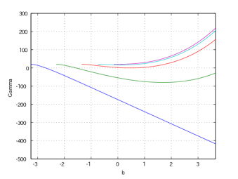
$\Gamma(a,\cdot)$	$\gamma(a,\cdot)$

Figure 1. Quadratic case: the plots of $b\mapsto\Gamma(a,b)$ (left) and $b\mapsto\gamma(a,b)$ (right) for $a=\underline{a},(\underline{a}+a^{*})/2,a^{*},(a^{*}+\overline{a})/2,\overline{a}$. The line in red corresponds to the one for $a=a^{*}$; the point at which $\Gamma(a^{*},\cdot)$ is tangent to the x-axis (or $\gamma(a^{*},\cdot)$ vanishes) becomes $b^{*}$.

In Figure 2, we show the value functions for $C_{U}\in E:=\{35,30,25,20,15,10,5,0,-5\}$ with the common value of $C_{D}=6$ (left) and also those for $C_{D}\in E$ with $C_{U}=6$ (right). With these selections of parameters, (2.3) is always satisfied. It is clear that the value function is monotone in both $C_{U}$ and $C_{D}$. The distance between $a^{*}$ and $b^{*}$ tends to shrink as $C_{U}+C_{D}$ decreases. In all cases, we can confirm that the optimal barrier levels $(a^{*},b^{*})$ are indeed finite.

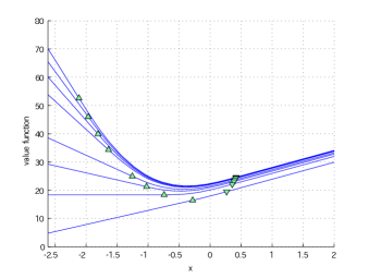
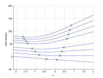
with respect to $C_{U}$	with respect to $C_{D}$

Figure 2. Quadratic case: the plots of the value function for $C_{U}\in E$ with the common value of $C_{D}=6$ (left) and also those for $C_{D}\in E$ with $C_{U}=6$ (right). The up-pointing and down-pointing triangles show the points at $a^{*}$ and $b^{*}$, respectively.

7.2. Linear case

We shall then consider the linear case with $f\equiv f_{L}$ as in (6.6) with $\alpha^{-}=\alpha^{+}=1$. Figure 3 shows the functions $b\mapsto\Gamma(a,b)$ and $b\mapsto\gamma(a,b)$ for $a=\underline{a},(\underline{a}+a^{*})/2,a^{*},(a^{*}+\overline{a})/2,\overline{a}$ with the common values $C_{U}=C_{D}=10$. A noticeable difference with the quadratic case in Figure 1 is that the function $\gamma(a,\cdot)$ is not differentiable at $b=0$. Moreover, $\Gamma(\underline{a},\cdot)$ converges to a finite value. Recall that the limit is positive if and only if $a^{*}=\underline{a}$ and $b^{*}=\infty$. We can confirm that Assumption 5.1 is indeed satisfied.

Similarly to Figure 2, we show in Figure 4 the value functions using the same parameter set for $C_{U}$ and $C_{D}$. Here, we exclude the case $C_{U}=35$ because it violates (6.7). Moreover, the case $C_{D}=35$ is an example of Case 2 because $C_{D}\geq\alpha^{+}/q$ as in Proposition 6.2. We see that because the tail of the function $f$ grows/decreases slower than the quadratic case, the levels $(a^{*},b^{*})$ for this linear case are more sensitive to the values of $C_{U}$ and $C_{D}$.

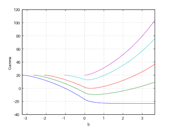
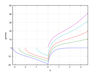
$\Gamma(a,\cdot)$	$\gamma(a,\cdot)$

Figure 3. Linear case: the plots of $b\mapsto\Gamma(a,b)$ (left) and $b\mapsto\gamma(a,b)$ (right) for $a=\underline{a},(\underline{a}+a^{*})/2,a^{*},(a^{*}+\overline{a})/2,\overline{a}$.

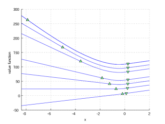
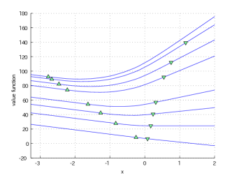
with respect to $C_{U}$	with respect to $C_{D}$

Figure 4. Linear case: the plots of the value function for $C_{U}\in E\backslash\{35\}$ with the common value of $C_{D}=6$ (left) and also those for $C_{D}\in E$ with $C_{U}=6$ (right). The largest function in the right plot shows the case with $C_{D}=35$ where the optimal barrier levels are given by $a^{*}=\underline{a}$ and $b^{*}=\infty$.

References

- [1] F. Avram, Z. Palmowski, and M. R. Pistorius. On the optimal dividend problem for a spectrally negative Lévy process. Ann. Appl. Probab., 17(1):156–180, 2007.
- [2] S. Baccarin. Optimal impulse control for cash management with quadratic holding-penalty costs. Decisions in Economics and Finance, 25(1):19–32, 2002.
- [3] E. J. Baurdoux and A. E. Kyprianou. The McKean stochastic game driven by a spectrally negative Lévy process. Electron. J. Probab., 13:no. 8, 173–197, 2008.
- [4] E. J. Baurdoux, A. E. Kyprianou, and J. C. Pardo. The Gapeev-Kühn stochastic game driven by a spectrally positive Lévy process. Stochastic Process. Appl., 121(6):1266–1289, 2008.
- [5] E. Bayraktar and M. Egami. An analysis of monotone follower problems for diffusion processes. Math. Oper. Res., 33(2):336–350, 2008.
- [6] E. Bayraktar, A. E. Kyprianou, and K. Yamazaki. On optimal dividends in the dual model. Astin Bull., 43(3):359–372, 2013.
- [7] E. Bayraktar, A. E. Kyprianou, and K. Yamazaki. Optimal dividends in the dual model under transaction costs. Insurance: Math. Econom., 54:133–143, 2014.
- [8] L. Benkherouf and A. Bensoussan. Optimality of an policy with compound Poisson and diffusion demands: a quasi-variational inequalities approach. SIAM J. Control Optim., 48(2):756–762, 2009.
- [9] A. Bensoussan, R. H. Liu, and S. P. Sethi. Optimality of an policy with compound Poisson and diffusion demands: a quasi-variational inequalities approach. SIAM J. Control Optim., 44(5):1650–1676, 2005.
- [10] J. Bertoin. Lévy processes, volume 121 of Cambridge Tracts in Mathematics. Cambridge University Press, Cambridge, 1996.
- [11] D. Beyer, S. P. Sethi, and M. Taksar. Inventory models with Markovian demands and cost functions of polynomial growth. J. Optim. Theory Appl., 98(2):281–323, 1998.
- [12] T. Chan, A. E. Kyprianou, and M. Savov. Smoothness of scale functions for spectrally negative Lévy processes. Probab. Theory Relat. Fields, 150:691–708, 2011.
- [13] G. M. Constantinides and S. F. Richard. Existence of optimal simple policies for discounted-cost inventory and cash management in continuous time. Oper. Res., 26(4):620–636, 1978.
- [14] J. Dai, D. Yao, et al. Brownian inventory models with convex holding cost, part 1: Average-optimal controls. Stochastic Systems, 3(2):442–499, 2013.
- [15] J. Dai, D. Yao, et al. Brownian inventory models with convex holding cost, part 2: Discount-optimal controls. Stochastic Systems, 3(2):500–573, 2013.
- [16] M. Egami, T. Leung, and K. Yamazaki. Default swap games driven by spectrally negative Lévy processes. Stochastic Process. Appl., 123(2):347–384, 2013.
- [17] M. Egami and K. Yamazaki. Precautionary measures for credit risk management in jump models. Stochastics, 85(1):111–143, 2013.
- [18] M. Egami and K. Yamazaki. Phase-type fitting of scale functions for spectrally negative Lévy processes. J. Comput. Appl. Math., 264:1–22, 2014.
- [19] G. D. Eppen and E. F. Fama. Cash balance and simple dynamic portfolio problems with proportional costs. International Economic Review, 10(2):119–133, 1969.
- [20] X. Guo and H. Pham. Optimal partially reversible investment with entry decision and general production function. Stochastic Process. Appl., 115(5):705–736, 2005.
- [21] J. M. Harrison and M. I. Taksar. Instantaneous control of Brownian motion. Math. Oper. Res., 8(3):439–453, 1983.
- [22] D. Hernandez-Hernandez and K. Yamazaki. Games of singular control and stopping driven by spectrally one-sided Lévy processes. Stochastic Process. Appl., forthcoming.
- [23] F. Hubalek and A. E. Kyprianou. Old and new examples of scale functions for spectrally negative Lévy processes. Sixth Seminar on Stochastic Analysis, Random Fields and Applications, eds R. Dalang, M. Dozzi, F. Russo. Progress in Probability, Birkhäuser, 2010.
- [24] I. Karatzas. The monotone follower problem in stochastic decision theory. Appl. Math. Optim., 7(1):175–189, 1981.
- [25] A. Kuznetsov. Wiener-Hopf factorization and distribution of extrema for a family of Lévy processes. Ann. Appl. Probab., 2009.
- [26] A. Kuznetsov, A. E. Kyprianou, and J. C. Pardo. Meromorphic Lévy processes and their fluctuation identities. Ann. Appl. Probab., 22(3):1101–1135, 2012.
- [27] A. Kuznetsov, A. E. Kyprianou, and V. Rivero. The theory of scale functions for spectrally negative levy processes. Springer Lecture Notes in Mathematics, 2061:97–186, 2013.
- [28] A. E. Kyprianou. Introductory lectures on fluctuations of Lévy processes with applications. Universitext. Springer-Verlag, Berlin, 2006.
- [29] A. E. Kyprianou and B. A. Surya. Principles of smooth and continuous fit in the determination of endogenous bankruptcy levels. Finance Stoch., 11(1):131–152, 2007.
- [30] R. L. Loeffen. On optimality of the barrier strategy in de Finetti’s dividend problem for spectrally negative Lévy processes. Ann. Appl. Probab., 18(5):1669–1680, 2008.
- [31] P. Matomäki. On solvability of a two-sided singular control problem. Math. Method Oper. Res., 76(3):239–271, 2012.
- [32] A. Merhi and M. Zervos. A model for reversible investment capacity expansion. SIAM J. Control Optim., 46(3):839–876, 2007.
- [33] M. R. Pistorius. On doubly reflected completely asymmetric Lévy processes. Stochastic Process. Appl., 107(1):131–143, 2003.
- [34] M. R. Pistorius. On exit and ergodicity of the spectrally one-sided Lévy process reflected at its infimum. J. Theoret. Probab., 17(1):183–220, 2004.
- [35] P. E. Protter. Stochastic integration and differential equations, volume 21 of Stochastic Modelling and Applied Probability. Springer-Verlag, Berlin, 2005. Second edition. Version 2.1, Corrected third printing.
- [36] S. P. Sethi and M. I. Taksar. Optimal financing of a corporation subject to random returns. Math. Finance, 12(2):155–172, 2002.
- [37] A. Sulem. A solvable one-dimensional model of a diffusion inventory system. Math. Oper. Res., 11(1):125–133, 1986.
- [38] K. Yamazaki. Inventory control for spectrally positive Lévy demand processes. arXiv:1303.5163, 2013.