Molecular gas content in strongly-lensed $z\sim 1.5-3$ star-forming galaxies with low IR luminosities

To extend the molecular gas measurements to more typical star-forming galaxies (SFGs) with ${\rm SFR}<40\leavevmode\nobreak\ \rm M_{\sun}\leavevmode\nobreak\ yr^{-1}$ and $M_{*}<2.5\times 10^{10}\leavevmode\nobreak\ \rm M_{\sun}$ at $z\sim 1.5-3$, we have observed CO emission with the IRAM Plateau de Bure Interferometer and 30 m telescope for five strongly-lensed galaxies, selected from the Herschel Lensing Survey. These observations are combined with a compilation of CO measurements from the literature. From this, we infer the CO luminosity correction factors $r_{2,1}=0.81\pm 0.20$ and $r_{3,1}=0.57\pm 0.15$ for the $J=2$ and $J=3$ CO transitions, respectively, valid for SFGs at $z>1$. The combined sample of CO-detected SFGs at $z>1$ shows a large spread in star formation efficiency (SFE) with a dispersion of 0.33 dex, such that the SFE extend well beyond the low values of local spirals and overlap the distribution of $z>1$ sub-mm galaxies. We find that the spread in SFE (or equivalently in molecular gas depletion timescale) is due to variations of several physical parameters, primarily the specific star formation rate, but also stellar mass and redshift. Correlations of the SFE with the offset from the main-sequence and the compactness of the starburst are less clear. The possible increase of the molecular gas depletion timescale with $M_{*}$ now revealed by low stellar mass SFGs at $z>1$ and also observed at $z=0$ is in contrast to the constant molecular gas depletion timescale generally admitted and refutes the linearity of the Kennicutt-Schmidt relation. A net rise of the molecular gas fraction ($f_{\rm gas}$) is observed from $z\sim 0.2$ to $z\sim 1.2$, followed by a very mild increase toward higher redshifts, as found in earlier studies. At each redshift the molecular gas fraction shows a large dispersion, mainly due to the dependence of $f_{\rm gas}$ on stellar mass, producing a gradient of increasing $f_{\rm gas}$ with decreasing $M_{*}$. We provide the first measurement of the molecular gas fraction of $z>1$ SFGs at the low-$M_{*}$ end between $10^{9.4}<M_{*}/{\rm M}_{\sun}<10^{9.9}$, reaching a mean $\langle f_{\rm gas}\rangle=0.69\pm 0.18$ which shows a clear $f_{\rm gas}$ upturn at these lower stellar masses. Finally, we find evidence for a non-universal dust-to-gas ratio among high-redshift SFGs and sub-mm galaxies, local spirals and ultra-luminous infrared galaxies with near-solar metallicities, as inferred from a homogeneous analysis of their rest-frame 850 $\mu$m luminosity per unit gas mass. $z>1$ SFGs show a trend for a lower $L_{\nu}(850\,\mu{\rm m})/M_{\rm gas}$ mean by 0.33 dex compared to the other galaxy populations.

1 Introduction

Gas, stars, dust, and metals are the basic galaxy constituents. They determine the majority of observable properties in galaxies at all wavelengths. Therefore, the characterization of these observable properties from present up to high-redshifts provides stringent tests and anchors for the physical processes that regulate the galaxy evolution.

Several empirical relationships between gas, stars, dust, and metals have been observationally identified. The first relationship is the correlation between the star formation rate (SFR) and stellar mass ($M_{*}$). It determines the so-called “main-sequence”, representing the locus where local and high-redshift star-forming galaxies (SFGs) lie in the SFR–$M_{*}$ plane. The correlation is slightly sublinear and evolves with redshift, such that high-redshift galaxies form more stars per unit time than the low-redshift ones with the same stellar mass (e.g., Noeske et al. 2007; Daddi et al. 2007; Elbaz et al. 2007; Rodighiero et al. 2010; Salmi et al. 2012). This implies an increase of the specific star formation rate, defined as the ratio of the star formation rate over the stellar mass, with redshift. The second relationship is the correlation between the gas-phase metallicity and stellar mass (e.g., Tremonti et al. 2004; Savaglio et al. 2005; Erb et al. 2006; Maiolino et al. 2008). It shows a redshift evolution toward lower metallicities at higher redshifts. More recently, Mannucci et al. (2010, 2011) found the “fundamental” metallicity relation (FMR) that connects at the same time metallicity, stellar mass, and star formation rate, as revealed by local and $z<2.5$ galaxies. The third important relationship is the Kennicutt-Schmidt relation, or the star-formation relation, that relates the star formation rate surface density to the total gas ($\rm H\,I+H_{2}$) surface density through a power law (Kennicutt 1998a). Mostly constrained by local galaxies so far (Leroy et al. 2008; Bigiel et al. 2008, 2011), the tightest correlation is observed between the star formation rate surface density and the H₂ gas surface density well parametrized by a linear relation, meaning that the molecular gas is being consumed at a constant rate within a molecular gas depletion timescale of about 1.5 Gyr. However, both the COLD GASS survey of local massive galaxies ($\log(M_{*}/{\rm M_{\sun}})>10$) from Saintonge et al. (2011) and the recent ALLSMOG survey of local low-mass galaxies ($9<\log(M_{*}/{\rm M_{\sun}})<10$) from Bothwell et al. (2014) show an increase of the molecular gas depletion timescale with stellar mass and thus bring evidence against a linear Kennicutt-Schmidt relation. A linear Kennicutt-Schmidt relation for the H₂ gas surface densities seems to hold for high-redshift SFGs, but with a much shorter molecular gas depletion timescale of about 0.7 Gyr (Tacconi et al. 2013), even though they are more gas-rich (e.g., Daddi et al. 2010a; Tacconi et al. 2010; Genzel et al. 2010). Finally, there is the relationship between the dust-to-gas ratio and metallicity seen in nearby galaxies (e.g., Issa et al. 1990; Dwek 1998; Edmunds 2001; Inoue 2003; Draine et al. 2007; Leroy et al. 2011). Attempts to measure the dust-to-gas ratios of high-redshift galaxies support a similar correlation, as well as a trend toward smaller dust-to-gas ratios at higher redshifts (Saintonge et al. 2013; Chen et al. 2013).

Most of these empirical correlations are both qualitatively and quantitatively consistent with the so-called “bathtub” model, which gives a good analytical representation of the gross features of the star-forming galaxy evolution (e.g., Bouché et al. 2010; Lagos et al. 2012; Lilly et al. 2013; Dekel & Mandelker 2014). Solely based on the equation of conservation of gas mass in a galaxy, this model assumes that galaxies lie in a quasi-steady state equilibrium, where their ability to form stars is regulated by the availability of gas replenished through the accretion rate dictated by cosmology and the amount of material they return into the intergalactic medium through gas outflows. The predicted redshift and mass dependences are the following (although slightly differing from authors to authors): the average gas accretion rate varies as $M_{\rm halo}^{1.1}(1+z)^{2.2}$, the specific star formation rate as $(1+z)^{2.2}$, the gas depletion timescale as $(1+z)^{-1.5}$, and the molecular gas fraction steadily increases with redshift and decreases with stellar mass. In agreement with cosmological hydrodynamic simulations from Davé et al. (2011, 2012), the latter, in addition, predict a decrease of the gas depletion timescale with the stellar mass, instead of a constant gas depletion timescale.

Improvements in the sensitivity of the IRAM Plateau de Bure Interferometer have made it possible over the last years to start getting a census of the molecular gas content in star-forming galaxies near the peak of the cosmic star formation activity. However, the samples of CO-detected objects at $z=1-1.5$ and $z=2-3$ are still small and confined to the high-SFR and high-$M_{*}$ end of main-sequence SFGs (Daddi et al. 2010a; Genzel et al. 2010; Tacconi et al. 2010, 2013). In this paper, we extend the dynamical range of star formation rates and stellar masses of star-forming galaxies with observationally constrained molecular gas contents below $\rm SFR<40\leavevmode\nobreak\ M_{\sun}\leavevmode\nobreak\ yr^{-1}$ and $M_{*}<2.5\times 10^{10}\leavevmode\nobreak\ \rm M_{\sun}$, and thus reach the $L^{\star}$ to sub-$L^{\star}$ domain of $z\sim 1.5-3$ galaxies (Gruppioni et al. 2013). This domain of physical parameters is accessible to CO emission measurements only with the help of gravitational lensing, a technique that proved to be efficient by a few objects already(Baker et al. 2004; Coppin et al. 2007; Saintonge et al. 2013). Therefore, our five galaxies selected for CO follow-up observations come from the Herschel Lensing Survey of massive galaxy cluster fields (HLS; Egami et al. 2010), designed to detect lensed, high-redshift background galaxies and probe more typical, intrinsically fainter galaxies than those identified in large-area, blank-field surveys. The gaseous, stellar, and dust properties inferred for these (sub-)$L^{\star}$ main-sequence star-forming galaxies (see also Sklias et al. 2014) are put face-to-face with a large comparison sample of local and high-redshift galaxies with CO measurements reported in the literature, which together provide new tests and anchors for galaxy evolution models.

In Sect. 2 we describe the target selection and their physical properties, and present the comparison sample of CO-detected galaxies from the literature. In Sect. 3 we report on CO observations performed with the IRAM Plateau de Bure Interferometer and 30 m telescope and discuss the CO results. In Sect. 4 we infer the CO luminosity correction factors for the $J=2$ and $J=3$ CO rotational transitions. The gaseous and stellar properties of our strongly-lensed galaxies are placed in the general context of galaxies with CO measurements in Sect. 5, where the main objective is to understand what drives the large spread in star formation efficiency observed in high-redshift SFGs. In Sect. 6 we explore the redshift evolution and the stellar mass dependence of their molecular gas fractions. In Sect. 7 we discuss the universality of the dust-to-gas ratio inferred from a homogeneous analysis of the rest-frame 850 $\mu$m continuum. Summary and conclusions are given in Sect. 8. Individual CO properties and inferred kinematics of our selected strongly-lensed galaxies are described in Appendix A.

Throughout the paper, we adopt the initial mass function (IMF) of Chabrier (2003) and scale the values from the literature by the factor of 1.7 when the Salpeter (1955) IMF is used. The designation to “gas” always refers to the molecular gas (H₂) only and not the total gas ($\rm H\,I+H_{2}$). All the molecular gas masses are derived from the observed CO emission via the “Galactic” CO(1–0)–H₂ conversion factor $X_{\rm CO}=2\times 10^{20}\leavevmode\nobreak\ \rm cm^{-2}/(K\leavevmode\nobreak\ km\leavevmode\nobreak\ s^{-1})$, or $\alpha=4.36\leavevmode\nobreak\ \rm M_{\sun}/(K\leavevmode\nobreak\ km\leavevmode\nobreak\ s^{-1}\leavevmode\nobreak\ pc^{2})$ which includes the correction factor of 1.36 for helium. We use the cosmology with $\rm H_{0}=70\leavevmode\nobreak\ km\leavevmode\nobreak\ s^{-1}\leavevmode\nobreak\ Mpc^{-1}$, $\Omega_{\rm M}=0.29$, and $\Omega_{\Lambda}=0.71$.

Table 1: Physical properties derived from SED fitting

Source	$z_{\rm H\alpha}$	$\mu$	$L_{\rm IR}$	$M_{*}$	SFR	$M_{\rm dust}$	$T_{\rm dust}$	$L_{\nu}(850\,\mu{\rm m})$
			($\rm 10^{11}\leavevmode\nobreak\ L_{\sun}$)	($\rm 10^{10}\leavevmode\nobreak\ M_{\sun}$)	($\rm M_{\sun}\leavevmode\nobreak\ yr^{-1}$)	($\rm 10^{7}\leavevmode\nobreak\ M_{\sun}$)	(K)	($\rm 10^{29}\leavevmode\nobreak\ erg\leavevmode\nobreak\ s^{-1}\leavevmode\nobreak\ Hz^{-1}$)
A68-C0	1.5864	30	$1.18\pm 0.07$	$2.0\pm 0.65$	$9^{+3.3}_{-3.9}$	4.7	34.5	5.0
A68-HLS115	1.5869	15	$3.42\pm 0.16$	$0.81^{+0.17}_{-0.20}$	$25^{+2.6}_{-6}$	3.0	37.5	7.7
MACS0451-arc	2.013	49	$1.36\pm 0.13$	$0.25\pm 0.02$	$19^{+0.6}_{-0.2}$	0.6	47.4	3.4
A2218-Mult	3.104	14	$2.26\pm 0.15$
A68-h7	2.15	3	$18.3^{+0.9}_{-1.2}$	$15.4^{+0.9}_{-3.8}$	$76\pm 3.4$	18.2	43.3	27.6
MS 1512-cB58	2.729	30	$3.04\pm 0.07$	$0.44\pm 0.03$	$37^{+2.4}_{-2.9}$	1.2	50.1	2.0
Cosmic Eye	3.0733	28	$3.41^{+0.16}_{-0.23}$	$2.4\pm 0.06$	$33\pm 0.6$	2.2	46.3	3.3

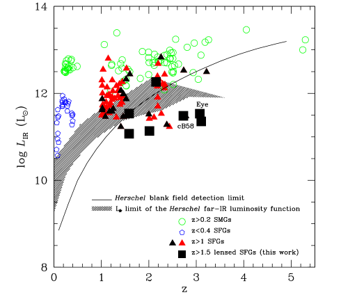
Figure 1: IR luminosities as a function of redshift of our low-$L_{\rm IR}$ selected SFGs (squares) compared to our compilation of galaxies with CO measurements from the literature (see Sect. 2.2). Symbols in black refer to $L_{\rm IR}$ as derived from the Herschel far-IR photometry. Our SFGs populate the regime with the lower $L_{\rm IR}$ reported at $z>1.5$: they reach the $L^{\star}$ and below domain as delimited by the hatched area showing the $L^{\star}$ limit of the Herschel far-IR luminosity function as determined by Magnelli et al. (2013, upper band) and Gruppioni et al. (2013, lower band) and extend the blank field studies to fainter luminosities as it is shown by the solid line which defines the minimal $L_{\rm IR}$ at each redshift that produces a flux $\gtrsim 2\leavevmode\nobreak\ \rm mJy$ in the Herschel/PACS 160 $\mu$m band ($\sim 3\,\sigma$ detection limit in GOODS-N, Elbaz et al. 2011).

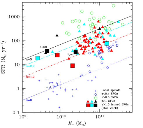
Figure 2: Location of our low-$L_{\rm IR}$ selected SFGs (squares) in the star-formation–stellar-mass plane compared to our compilation of galaxies with CO measurements from the literature (see Sect. 2.2). Our (sub-)$L^{\star}$ galaxies probe one order of magnitude smaller stellar masses than the bulk of $z>1$ SFGs from the literature. The blue dotted, red short-dashed, cyan long-dashed, and black solid lines are the best-fits of SFR–$M_{*}$ MS at $z\simeq 0$, 1.2, 2.2, and 3, respectively, parametrized by Eq. (2.1). The color-coding of SFGs (our sample plus the $z>1$ SFGs from the literature) refers to three redshift intervals: $\langle z_{1.2}\rangle=[1,1.6]$ (red), $\langle z_{2.2}\rangle=[2,2.5]$ (cyan), and $\langle z_{3.0}\rangle=[2.7,3.2]$ (black) in line with the MS fits.

2 High-redshift samples of CO-detected galaxies

2.1 Target selection

The HLS is providing us with unique targets ideal for CO follow-up studies. We used this dataset to select galaxies at $z\sim 1.5-3$ with low intrinsic (delensed) IR luminosities $L_{\rm IR}<4\times 10^{11}\leavevmode\nobreak\ \rm L_{\sun}$, as derived from the Herschel/PACS (100 and 160 $\mu$m) and SPIRE (250, 350, and 500 $\mu$m) SED modelling. These galaxies are of particular interest, because they allow probing the molecular gas content at high redshift in a regime of star formation rates $\rm SFR<40\leavevmode\nobreak\ M_{\sun}\leavevmode\nobreak\ yr^{-1}$ still very poorly explored, while being typical of “normal” star-forming galaxies. In addition, we required that our targets (1) are strongly lensed with well-known magnification factors derived from robust lens modelling (Richard et al. 2007, 2011) in order to make the CO emission of these intrinsically faint $L_{\rm IR}$ objects accessible to current millimeter instruments, (2) have known spectroscopic redshifts from our optical and near-IR observing campaigns (Richard et al. 2007, 2011), (3) have well-sampled global SEDs from optical, near-IR to IR obtained with ground-based telescopes, the Hubble Space Telescope (HST), and the Spitzer satellite in order to have tight estimates of their stellar masses and star formation rates, and (4) have high-resolution HST images useful to get information on their morphology.

The four galaxies—A68-C0, A68-HLS115, MACS0451-arc, and A2218-Mult—selected for CO observations with the IRAM interferometer at the Plateau de Bure, France, do satisfy all the above specifications. The fifth object—A68-h7— observed with the IRAM 30 m telescope at Pico Veleta, Spain, has a higher intrinsic IR luminosity and hence has properties resembling more the high-redshift galaxies with CO measurements already available. A description of these selected targets at $z>1.5$, as well as their detailed multi-wavelength SED analysis from optical to far-IR/sub-mm can be found in Sklias et al. (2014, except for A2218-Mult). In Table 1 we summarize their physical properties: spectroscopic redshifts ($z_{\rm H\alpha}$), magnification factors ($\mu$), IR luminosities ($L_{\rm IR}$), stellar masses ($M_{*}$), star formation rates (SFR), dust masses ($M_{\rm dust}$), dust temperatures ($T_{\rm dust}$), and rest-frame 850 $\mu$m luminosities ($L_{\nu}(850\,\mu{\rm m})$). We add to this sample, MS 1512-cB58 (Yee et al. 1996, hereafter ‘cB58’) and the Cosmic Eye (Smail et al. 2007, hereafter ‘Eye’), two well-known strongly-lensed galaxies with similar characteristics, for which we provide in Sklias et al. (2014) revised physical properties obtained from updated SED fitting and Herschel photometry.

In Fig. 1 we show the intrinsic IR luminosities of the low-$L_{\rm IR}$ selected SFGs as a function of redshift and compare them to the compilation of galaxies with CO measurements from the literature (Sect. 2.2). Our sample of SFGs populates the regime with the lower $L_{\rm IR}$ reported at $z>1.5$ as expected from the selection criterion and reach the $L^{\star}$ to sub-$L^{\star}$ domain according to the Herschel far-IR luminosity function of galaxies at $z\sim 1.5-3$ with $\log(L^{\star}/{\rm L}_{\sun})$ varying between 11.4 and 12.3 (see the hatched area in Fig. 1 as delimited from Gruppioni et al. (2013) and Magnelli et al. (2013)). These $L_{\rm IR}$, derived from Herschel far-IR photometry, also fall below the Herschel detection limit and are only accessible with gravitational lensing. All the data points from the literature below the Herschel detection limit refer either to other lensed galaxies with Herschel $L_{\rm IR}$ measurements or to galaxies with $L_{\rm IR}$ measurements determined from their star formation rates via the Kennicutt (1998b) relation, $L_{\rm IR}\leavevmode\nobreak\ \rm(L_{\sun})=10^{10}\times SFR\leavevmode\nobreak\ (M_{\sun}\leavevmode\nobreak\ yr^{-1})$, scaled to the Chabrier (2003) IMF.

Our sample of strongly-lensed galaxies also probes very small stellar masses $M_{*}<2.5\times 10^{10}\leavevmode\nobreak\ \rm M_{\sun}$ (see Table 1), on average one order of magnitude smaller compared to the stellar masses of the bulk of $z>1$ SFGs with CO measurements reported in the literature; making our sample of particular interest for the study of the molecular gas content in a new regime of smaller stellar masses in addition to the lower star formation  rates. This is in line with the well-defined empirical SFR–$M_{*}$ relation. Our galaxies indeed nicely follow the main-sequence (MS) of $z\simeq 1.2$, 2.2, and 3 galaxies, respectively, as shown in Fig. 2. We consider here the best-fit parametrization of the SFR–$M_{*}$ MS given by Tacconi et al. (2013) based on the samples of Bouché et al. (2010), Noeske et al. (2007), Daddi et al. (2007), Rodighiero et al. (2010), and Salmi et al. (2012):

$${\rm SFR_{MS}}(z,M_{*})\leavevmode\nobreak\ {\rm(M_{\sun}\leavevmode\nobreak\ yr^{-1})} =$$

$$45(M_{*}/6.6\times 10^{10}\leavevmode\nobreak\ ({\rm M_{\sun}}))^{0.65}((1+z)/2.2)^{2.8}\,,$$ (1)

which we compute at three redshifts, the redshift medians of our comparison sample of CO-detected $z>1$ SFGs from the literature (Sect. 2.2), plus our sample of low-$L_{\rm IR}$ selected galaxies, within three redshift intervals: $\langle z_{1.2}\rangle=[1,1.6]$, $\langle z_{2.2}\rangle=[2,2.5]$, and $\langle z_{3.0}\rangle=[2.7,3.2]$. No excess in the specific star formation rate is observed among our objects, they all lie within $0.3<{\rm sSFR/sSFR_{MS}}\equiv\frac{{\rm SFR}/M_{*}}{{\rm SFR_{MS}}/M_{*}}<3$, the admitted thickness of the main-sequence (e.g., Magdis et al. 2012b). On the other hand one galaxy—the Eye—is located below the MS at its respective redshift with $\rm sSFR/sSFR_{MS}=0.27$.

2.2 Comparison sample

In order to have a comparison sample to put face to face with our sample of low-$L_{\rm IR}$ selected galaxies, we built up a large compilation of local and high-redshift galaxies with CO measurements reported in the literature. We refer to the same comparison sample throughout the paper. This compilation is exhaustive for star-forming galaxies that have the highest priority in the comparative work to our sample of galaxies, very complete for high-redshift sub-mm galaxies (SMGs), but remains incomplete for all local galaxies including the spiral galaxies, luminous IR galaxies (LIRGs), and ultra-luminous IR galaxies (ULIRGs). All these CO-detected galaxies are classified along the following sub-categories and are designated by the same symbols (but not by the same colors) in all figures.

• Local spirals with $L_{\rm IR}<10^{11}\leavevmode\nobreak\ \rm L_{\sun}$ (crosses):
  Helfer et al. (2003), Gao & Solomon (2004), Leroy et al. (2008, 2009), Papadopoulos et al. (2012), Wilson et al. (2012), and Bothwell et al. (2014).
  

• Local LIRGs with $10^{11}<L_{\rm IR}<10^{12}\leavevmode\nobreak\ \rm L_{\sun}$ (filled diamonds):
  Solomon et al. (1997), Gao & Solomon (2004), Wilson et al. (2008), Leech et al. (2010), and Papadopoulos et al. (2012).
  

• Local ULIRGs with $L_{\rm IR}>10^{12}\leavevmode\nobreak\ \rm L_{\sun}$ (small open circles):
  Solomon et al. (1997) and Papadopoulos et al. (2012).
  

• High-redshift SMGs/ULIRGs at $z>0.2$ with $L_{\rm IR}>10^{12}\leavevmode\nobreak\ \rm L_{\sun}$ (big open circles):
  Greve et al. (2005), Kneib et al. (2005), Iono et al. (2006), Tacconi et al. (2006), Daddi et al. (2009a, b), Knudsen et al. (2009), Weiss et al. (2009), Bothwell et al. (2010, 2013), Carilli et al. (2010), Harris et al. (2010), Ivison et al. (2010, 2011), Riechers et al. (2010, 2011), Swinbank et al. (2010), Yan et al. (2010), Braun et al. (2011), Casey et al. (2011), Combes et al. (2011, 2012, 2013), Danielson et al. (2011), Fu et al. (2012), Sharon et al. (2013), Rawle et al. (2014), and Magdis et al. (2014).
  

• SFGs at $z<0.4$ (open pentagons) and at $z>1$ (filled triangles) including field and lensed galaxies:
  Dannerbauer et al. (2009), Geach et al. (2009), Geach et al. (2011), Knudsen et al. (2009), Aravena et al. (2010, 2012, 2014), Genzel et al. (2010), Tacconi et al. (2010, 2013), Daddi et al. (2010a, 2014), Johansson et al. (2012), Magdis et al. (2012a, b), Magnelli et al. (2012), Bauermeister et al. (2013), Saintonge et al. (2013), Tan et al. (2013), and Magdis et al. (2014).

Table 2: Observation summary

Source	Coordinates		$T_{\rm on-source}$	CO	$\nu_{\rm obs}$	Synthesized beam		Bandwidth	rms
	RA (J2000)	DEC (J2000)	(hours)	line	(GHz)	Size ($\arcsec$)	PA ($\degr$)	(MHz)	(mJy)
A68-C0	00:37:07.404	+09:09:26.57	5.2	2–1	89.131	$6.41\times 5.53$	174	15	0.72
A68-HLS115	00:37:09.503	+09:09:03.80	4.6	2–1	89.128	$5.94\times 5.79$	111	15	0.71
MACS0451-arc	04:51:57.093	+00:06:10.44	30.2	3–2	114.768	$5.45\times 4.12$	163	19	0.84
A2218-Mult	16:35:48.919	+66:12:13.81	9.2	3–2	84.258	$6.35\times 5.90$	90	15	0.77
A68-h7	00:37:01.41	+09:10:22.31	5.5	3–2	109.777			24	0.94

Table 3: CO emission properties

Source	$z_{\rm CO}$	CO	$\rm S/N_{det}$	$\rm FWHM_{CO}$	$F_{\rm CO}$	$L^{\prime}_{\rm CO(1-0)}$	$M_{\rm gas}$	$f_{\rm gas}$
		line		(km s-1)	(Jy km s-1)	($10^{9}\leavevmode\nobreak\ \rm K\leavevmode\nobreak\ km\leavevmode\nobreak\ s^{-1}\leavevmode\nobreak\ pc^{2}$)	($10^{10}\leavevmode\nobreak\ \rm M_{\sun}$)
A68-C0	1.5854	2–1	11	$334\pm 76$	$1.89\pm 0.28$	$2.6\pm 0.4$	1.2	0.38
A68-HLS115	1.5859	2–1	14	$267\pm 18$	$2.00\pm 0.30$	$5.5\pm 0.9$	2.4	0.75
MACS0451-arc	2.0118	3–2	4–5	$261\pm 41$	$1.27\pm 0.32$	$1.0\pm 0.3$	0.4	0.62
A2218-Mult	3.104	3–2	undetected	–	$<0.62$	$<3.8$	$<1.7$
A68-h7	2.1529	3–2	3–4	$282\pm 61$	$1.12\pm 0.22$	$16.9\pm 3.3$	7.4	0.33
MS 1512-cB58	2.727	1–0		174	$0.052\pm 0.013$	$0.6\pm 0.15$	0.3	0.41
Cosmic Eye	3.074	1–0		200	$0.077\pm 0.013$	$1.2\pm 0.2$	0.5	0.18

3 Observations, data reduction, and results

3.1 Plateau de Bure data

Table 2 summarizes the IRAM Plateau de Bure Interferometer (PdBI) observations of the galaxies—A68-C0, A68-HLS115, MACS0451-arc, and A2218-Mult—selected from the HLS with intrinsic $L_{\rm IR}<4\times 10^{11}\leavevmode\nobreak\ \rm L_{\sun}$. The observations were conducted under typical summer conditions between June and September 2011 using 5 antennas in the compact D-configuration. The compact D-configuration provides the highest sensitivity with the smallest spatial resolution ($\sim 5.5^{\prime\prime}$ at our typical tuned frequencies), which is ideal for detection projects. The frequencies were tuned to the expected redshifted frequency of the CO(2–1) or CO(3–2) line chosen according to the redshift of the targets in order to perform all the observations in the 3 mm band. On-source integration times were varying between 5 hours and 30 hours in the extreme case of MACS0451-arc. We used the WideX correlator that provides a continuous frequency coverage of 3.6 GHz in dual-polarization with a fixed channel spacing of 1.95 MHz resolution.

Standard data reduction was performed using the IRAM GILDAS software packages CLIC and MAP, where bandpass calibration was done using observations of calibrators that were best adapted to each of our targets individually. All data were mapped with the CLEAN procedure using the “clark” deconvolution algorithm and combined with “natural” weighting, resulting in synthesized beams listed in Table 2. The final noise per beam in all our cleaned, weighted images reaches an rms between 0.71 and 0.84 mJy over a resolution of 15 MHz ($50\leavevmode\nobreak\ \rm km\leavevmode\nobreak\ s^{-1}$). The velocity-integrated maps of the CO emission are obtained by averaging the cleaned, weighted images over the spectral channels where emission is detected, and the corresponding spectra are obtained by spatially integrating the cleaned, weighted images over the $1\,\sigma$ CO detection contours.

3.2 30 m telescope data

Table 2 also summarizes the IRAM 30 m telescope observations of the HLS source—A68-h7—undertaken on September 3-5, 2011 under good summer conditions. We used the four single pixel heterodyne EMIR receivers, two centred on the E0 band (3 mm) and two on the E1 band (2 mm) tuned, respectively, to the redshifted frequencies of the CO(3–2) and CO(4–3) lines. The data were recorded using the WILMA autocorrelator providing a spectral resolution of 2 MHz. The observations were conducted in wobbler-switching mode, with a switching frequency of 0.5 Hz and a symmetrical azimuthal wobbler throw of $50^{\prime\prime}$ to maximize the baseline stability. Series of 12 ON/OFF subscans of 30 seconds each were performed and calibrations were repeated every 6 minutes. A total on-source integration time of 5.5 hours was obtained on this target.

The data reduction was completed with the IRAM GILDAS software package CLASS. The scans obtained with the two receivers tuned on the CO(3–2) line were averaged using the temporal scan length as weight. The resulting 3 mm spectrum was then Hanning smoothed to a resolution of 24 MHz ($65\leavevmode\nobreak\ \rm km\leavevmode\nobreak\ s^{-1}$) and reaches an rms noise level of 0.94 mJy.

                             

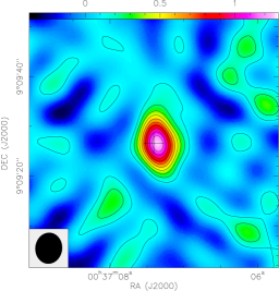
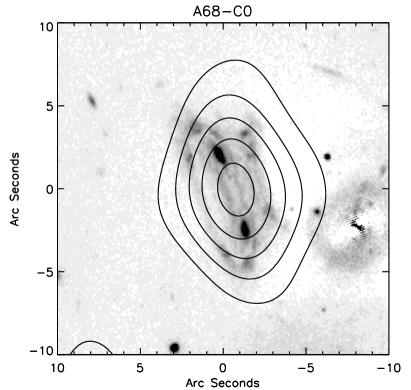
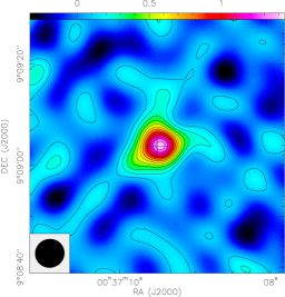
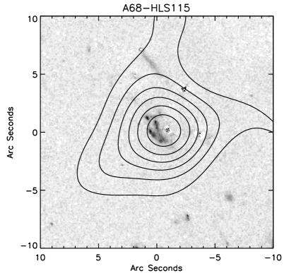
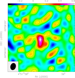
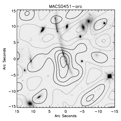
Figure 3: From top to bottom, we plot A68-C0, A68-HLS115 and MACS0451-arc. Left panels: Velocity-integrated, cleaned maps of the CO(2–1) or CO(3–2) emission detected in three of our low-$L_{\rm IR}$ selected galaxies observed with the PdBI. The maps are integrated over the cyan-shaded channels shown in Fig. 4. Contour levels start at $\pm 1\,\sigma$ and are in steps of $1\,\sigma$. The size and orientation of the beam is indicated by the black ellipse in the bottom left corner. None of these three CO detections is spatially resolved. The cross in each pannel corresponds to the coordinates of the optical HST continuum position as listed in Table 2 and is $\pm 2\arcsec$ ($\pm 17\leavevmode\nobreak\ \rm kpc$ at $z\simeq 2$) in size. The coding of the color bar is in units of integrated flux $\rm Jy\leavevmode\nobreak\ km\leavevmode\nobreak\ s^{-1}$. Right panels: CO(2–1) or CO(3–2) contours overlaid on the HST images in the F110W band for A68-C0, the F702W band for A68-HLS115, and the F140W band for MACS0451-arc. Contour levels start at $\pm 2\,\sigma$ and are in steps of $2\,\sigma$, except for MACS0451-arc where they start at $\pm 1\,\sigma$ and are in steps of $1\,\sigma$.

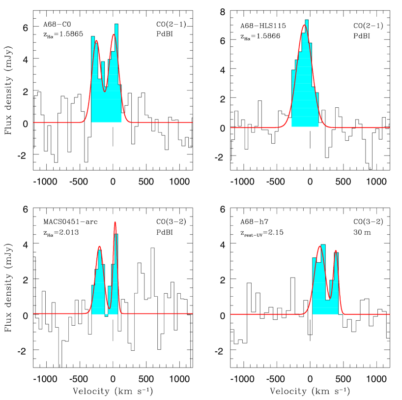
Figure 4: Spectra of the CO(2–1) or CO(3–2) emission line detected in our low-$L_{\rm IR}$ selected galaxies, binned in steps of $50\leavevmode\nobreak\ \rm km\leavevmode\nobreak\ s^{-1}$ except for A68-h7 where bins have a resolution of $65\leavevmode\nobreak\ \rm km\leavevmode\nobreak\ s^{-1}$. The cyan-shaded regions indicate channels where positive emission is detected. These channels have been used to derive total CO integrated fluxes and velocity-integrated maps shown in Fig. 3. The solid red lines are the best-fitting single or double Gaussian profiles to the observed CO line profiles. The zero velocity marked by the vertical bar corresponds to the tuning frequency of our targets listed in Table 2 and derived from the H$\alpha$ line or rest-frame UV absorption lines redshifts.

3.3 CO results

The CO emission has been successfully detected at the expected frequency for four out of the five low-$L_{\rm IR}$ selected galaxies, it remains undetected in A2218-Mult. CO velocity-integrated maps are shown in the left panels of Fig. 3 for the three positive detections obtained with PdBI. In the right panels of Fig. 3 we show the CO contours overlaid on the HST images of the corresponding galaxies. None of these three CO detections is spatially resolved, the observed spatial extension of the CO emission in our objects is similar to the PdBI beam size.

The resulting spectra of the CO detections can be found in Fig. 4. There is no evidence for continuum in any of our targets. The properties of the CO emission—velocity centroid ($z_{\rm CO}$), the line full width half maximum ($\rm FWHM_{CO}$), and the observed integrated line flux ($F_{\rm CO}$)—are evaluated by applying a single or double Gaussian fitting procedure on the observed line profiles based on the nonlinear $\chi^{2}$ minimization and the Levenberg-Marquardt algorithm. Errors on the values of $z_{\rm CO}$, $\rm FWHM_{CO}$, and $F_{\rm CO}$ are estimated using a Monte Carlo approach, whereby the observed spectrum is perturbed with a random realization of the error spectrum and refitted. The process is repeated 1000 times and the error in each quantity is taken to be the standard deviation of the values generated by the 1000 Monte Carlo runs. The derived best-fitting results are shown in Fig. 4. In addition to the measure of CO line integrated fluxes from spectra, we have obtained independent integrated flux measurements for A68-C0, A68-HLS115 and MACS0451-arc by fitting either a circular or elliptical Gaussian model to the two-dimensional CO emission observed in velocity-integrated maps. The two respective methods lead to consistent integrated CO line fluxes within $1\,\sigma$ errors.

Table 3 summarizes the measured CO emission properties. To convert the measured CO(2–1) and CO(3–2) luminosities to the fundamental CO(1–0) luminosity, which at the end gives a measure of the total H₂ mass, we apply the luminosity correction factors r${}_{2,1}=L^{\prime}_{\rm CO(2-1)}/L^{\prime}_{\rm CO(1-0)}=0.81\pm 0.20$ and r${}_{3,1}=L^{\prime}_{\rm CO(3-2)}/L^{\prime}_{\rm CO(1-0)}=0.57\pm 0.15$ to account for the lower Rayleigh-Jeans brightness temperature of the 2–1 and 3–2 transitions relative to 1–0, as determined in Sect. 4. To estimate the uncertainties on the luminosities, we simply propagate the uncertainties on the CO line integrated fluxes. The molecular gas masses, $M_{\rm gas}$, and gas fractions, $f_{\rm gas}=M_{\rm gas}/(M_{\rm gas}+M_{*})$, correspond to values computed with the “Galactic” CO–H₂ conversion factor $X_{\rm CO}=2\times 10^{20}\leavevmode\nobreak\ \rm cm^{-2}/(K\leavevmode\nobreak\ km\leavevmode\nobreak\ s^{-1})$, or $\alpha=4.36\leavevmode\nobreak\ \rm M_{\sun}/(K\leavevmode\nobreak\ km\leavevmode\nobreak\ s^{-1}\leavevmode\nobreak\ pc^{2})$ which includes the correction factor of 1.36 for helium. In the case of the CO(3–2) non-detection in A2218-Mult, we provide the $4\,\sigma$ upper limits computed from the rms noise achieved in the PdBI observations of this galaxy and assume a typical full width half maximum $\rm FWHM_{CO}=200\leavevmode\nobreak\ \rm km\leavevmode\nobreak\ s^{-1}$. The CO properties and inferred kinematics of the individual low-$L_{\rm IR}$ selected targets are described in Appendix A.

4 CO luminosity correction factors

The measure of the molecular gas mass requires the luminosity of the fundamental CO(1–0) line, $L^{\prime}_{\rm CO(1-0)}$. Nevertheless, as soon as we are interested in objects at $z>0.4$, accessing the fundamental CO(1–0) line at 115.27 GHz becomes impossible with mm/sub-mm receivers, and CO(1–0) must be replaced by rotationally excited $J>1$ CO transitions. Consequently, corrections for the ratio of the intrinsic Rayleigh-Jeans brightness temperatures in the 1–0 line to that in the rotationally excited line become necessary and need to be determined to access the fundamental $L^{\prime}_{\rm CO(1-0)}$. The corresponding CO luminosity correction factors vary with the $J$-transition of the CO line considered, the optical thickness, the thermal excitation and gas density of the medium, and hence the galactic type and redshift (Papadopoulos et al. 2012; Lagos et al. 2012; Narayanan et al. 2014).

Large efforts are done to get measurements of CO(1–0) and high-$J$ CO lines within the same objects to determine the CO spectral line energy distribution (SLED) of local and high-redshift galaxies (e.g., Weiss et al. 2007; Dannerbauer et al. 2009; Papadopoulos et al. 2010; Daddi et al. 2014). The comparison sample of CO-detected galaxies from the literature (Sect. 2.2), particularly exhaustive at high redshift, offers a unique opportunity to obtain a comprehensive view on the CO luminosity correction factors, defined as r${}_{J,1}=L^{\prime}_{{\rm CO}(J-(J-1))}/L^{\prime}_{{\rm CO}(1-0)}$, for the $J=2$ and $J=3$ CO rotational transitions. In Fig. 5 we plot the r_2,1 and r_3,1 correction factors as a function of the IR luminosity for galaxies from the comparison sample. The histograms show, respectively, r_2,1 and r_3,1 separately for $z=0$ galaxies (open histograms) and $z>1$ galaxies (hatched histograms), and for three $L_{\rm IR}$ intervals: $L_{\rm IR}<10^{11}\leavevmode\nobreak\ \rm L_{\sun}$ (the ‘spiral’ regime), $10^{11}\leavevmode\nobreak\ {\rm L}_{\sun}<L_{\rm IR}<10^{12}\leavevmode\nobreak\ {\rm L}_{\sun}$ (the ‘LIRG’ regime), and $L_{\rm IR}>10^{12}\leavevmode\nobreak\ \rm L_{\sun}$ (the ‘ULIRG’ regime).

The mean $\langle\rm r_{2,1}\rangle>0.9$ and $\langle\rm r_{3,1}\rangle\simeq 0.55-0.6$ values of $z=0$ galaxies within the ‘spiral’ and ‘LIRG’ regimes reveal relatively well-excited CO(2–1) and CO(3–2) lines. The observed luminosity correction factors are in line with the $1\gtrsim\rm r_{2,1}\gtrsim r_{3,1}\gtrsim r_{4,1}\gtrsim...$ sequence which is expected if the average state is dominated by one warm optically thick and thermally excited phase (Papadopoulos et al. 2012). On the other hand, $z=0$ galaxies within the ‘ULIRG’ regime show a predominance of a high-excitation phase with $\langle\rm r_{3,1}\rangle\gtrsim\langle r_{2,1}\rangle$ and a mean $\langle\rm r_{3,1}\rangle$ close to unity. This suggests highly-excited media and optically thin CO SLEDs in the higher $L_{\rm IR}$ $z=0$ galaxies. This view is supported by the models of Lagos et al. (2012) that predict flatter CO SLEDs for the brightest IR galaxies than for the fainter IR counterparts at $z=0$.

For $z>1$ galaxies the available r_2,1 and r_3,1 statistics is still small, except for r_3,1 within the ‘ULIRG’ regime. Both in the ‘LIRG’ and ‘ULIRG’ regimes, the mean $\langle\rm r_{2,1}\rangle\simeq 0.8$ and $\langle\rm r_{3,1}\rangle\simeq 0.6$ values point toward a slightly lower-excitation medium in high-redshift galaxies compared to $z=0$ galaxies, where the higher-$J$ CO lines are fainter as the subthermal excitation sets in more rapidly. The r_3,1 correction factors within the ‘ULIRG’ regime also show no significant sign of evolution toward higher excitation in the higher $L_{\rm IR}$ $z>1$ galaxies, unlike what is observed in $z=0$ galaxies. These results again are in a nice agreement with the models of Lagos et al. (2012) that predict (1) shallower CO SLEDs for high-redshift galaxies compared to their $z=0$ counterparts at a fixed IR luminosity, and (2) smaller differences in the CO SLEDs of faint- and bright-IR galaxies at $z>1$ than for $z=0$ galaxies. This is due to the increasing average gas kinetic temperature in molecular clouds with redshift. Given the fact that the observed high-$J$ CO transitions of our sample of $z>1$ galaxies are on average not highly excited, we may consider the “Galactic” CO–H₂ conversion factor as a sensible assumption for both SFGs and SMGs at $z>1$.

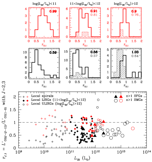
Figure 5: Bottom panel: Luminosity correction factors, r${}_{2,1}=L^{\prime}_{\rm CO(2-1)}/L^{\prime}_{\rm CO(1-0)}$ (in red) and r${}_{3,1}=L^{\prime}_{\rm CO(3-2)}/L^{\prime}_{\rm CO(1-0)}$ (in black), plotted as a function of the IR luminosity for galaxies from our comparison sample (see Sect. 2.2). Upper, middle panels: r_2,1 and r_3,1 distributions, respectively, of $z=0$ galaxies (open histograms) and $z>1$ galaxies (hatched histograms) plotted for three $L_{\rm IR}$ intervals: from left to right $L_{\rm IR}<10^{11}\leavevmode\nobreak\ \rm L_{\sun}$ (the ‘spiral’ regime), $10^{11}\leavevmode\nobreak\ {\rm L}_{\sun}<L_{\rm IR}<10^{12}\leavevmode\nobreak\ {\rm L}_{\sun}$ (the ‘LIRG’ regime), and $L_{\rm IR}>10^{12}\leavevmode\nobreak\ \rm L_{\sun}$ (the ‘ULIRG’ regime). The numbers in the upper right corner of each panel are the mean values of the r_J,1 distributions (“thick” numbers refer to $z=0$ galaxies and “thin” numbers to $z>1$ galaxies).

Throughout the paper, we adopt the following luminosity correction factors for SFGs (including our low-$L_{\rm IR}$ selected galaxies) at $z>1$: r${}_{2,1}=L^{\prime}_{{\rm CO}(2-1)}/L^{\prime}_{{\rm CO}(1-0)}=0.81\pm 0.20$ and r${}_{3,1}=L^{\prime}_{{\rm CO}(3-2)}/L^{\prime}_{{\rm CO}(1-0)}=0.57\pm 0.15$. These are the means of observed luminosity correction factors as measured at high redshift, instead of extrapolations from partial CO SLEDs or CO luminosity correction factors derived for local galaxies. Compared to the canonical value r${}_{3,1}=0.5$ assumed in the literature for $z>1$ SFGs (Tacconi et al. 2013; Saintonge et al. 2013), our r_3,1 value is 14% higher, but well within $1\,\sigma$. The difference between our r_2,1 value and the values found in the literature for $z>1$ SFGs is smaller: r${}_{2,1}=0.84$ in Daddi et al. (2010a) and r${}_{2,1}=0.75$ in Magnelli et al. (2012). The luminosity correction factors we derived for both high-redshift SFGs and SMGs also well agree with the values compiled by Carilli & Walter (2013), although based on other prescriptions for the $z>1$ SFGs.

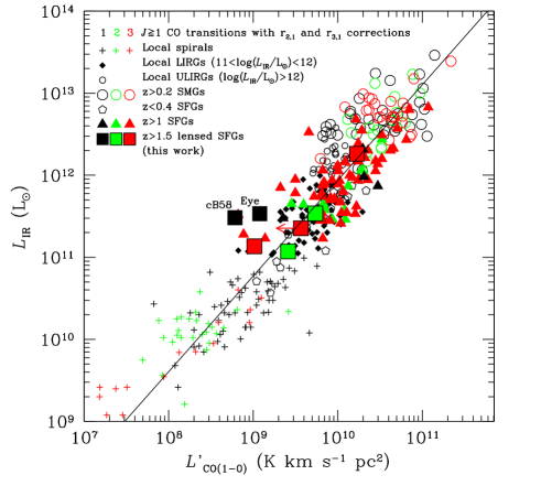
Figure 6: IR luminosities as a function of CO(1–0) luminosities of our low-$L_{\rm IR}$ selected SFGs (squares) compared to our compilation of galaxies with CO measurements from the literature (see Sect. 2.2). The color-coding of the various symbols refers to the $J=1$, 2, and 3 CO transitions used to infer $L^{\prime}_{\rm CO(1-0)}$ by applying the CO luminosity correction factors determined in Sect. 4. The best-fitting bisector linear relation to the entire sample of galaxies, $\log(L_{\rm IR})=(1.17\pm 0.03)\log(L^{\prime}_{\rm CO(1-0)})+(0.28\pm 0.23)$, is plotted as a solid line. The $z>1$ SFGs have on average a scatter in $L_{\rm IR}$ as large as 1 dex at a given value of $L^{\prime}_{\rm CO(1-0)}$ and a $1\,\sigma$ dispersion of 0.38 dex in the $y$-direction about the best-fitting $L_{\rm IR}$–$L^{\prime}_{\rm CO(1-0)}$ relation.

5 Low-$L_{\rm IR}$ selected galaxies in the general context of galaxies with CO measurements

We discuss the overall physical properties derived from the new CO measurements achieved in our low-$L_{\rm IR}$ selected galaxies. We combine and compare their CO luminosities, IR luminosities, star formation efficiencies, and molecular gas depletion timescales to our compilation of CO-detected galaxies from the literature (Sect. 2.2). The goal is to investigate whether the extended dynamical range toward lower star formation rates $\rm SFR<40\leavevmode\nobreak\ M_{\sun}\leavevmode\nobreak\ yr^{-1}$ and smaller stellar masses $M_{*}<2.5\times 10^{10}\leavevmode\nobreak\ \rm M_{\sun}$ shows evidence for new trends and correlations.

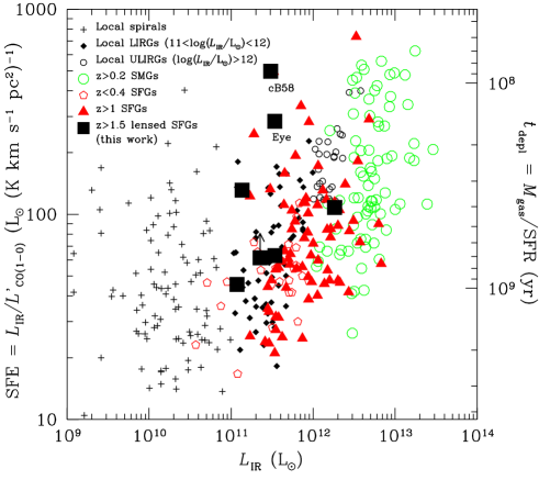
Figure 7: Star formation efficiencies, ${\rm SFE}=L_{\rm IR}/L^{\prime}_{\rm CO(1-0)}$ (left y-axis), or molecular gas depletion timescales, $t_{\rm depl}=M_{\rm gas}/{\rm SFR}$, assuming a “Galactic” CO–H₂ conversion factor for all galaxies (right y-axis), as a function of IR luminosities of our low-$L_{\rm IR}$ selected SFGs (squares) compared to our compilation of galaxies with CO measurements from the literature (see Sect. 2.2). This illustrates in another way the large dispersion about the $L_{\rm IR}$–$L^{\prime}_{\rm CO(1-0)}$ relation observed in Fig. 6.

5.1 CO luminosity to IR luminosity relation

It is now well established that there is a relation between $L_{\rm IR}$ and $L^{\prime}_{\rm CO(1-0)}$ (see the review by Carilli & Walter 2013) and this despite the uncertainties on $L^{\prime}_{\rm CO(1-0)}$ mostly inferred from higher $J>1$ CO rotational transitions and on $L_{\rm IR}$ often derived from various star formation tracers (UV, H$\alpha$, mid-IR, sub-mm, or radio) instead of direct far-IR photometry. The first high-redshift datasets showed evidence for a ‘bimodal’ $L_{\rm IR}$–$L^{\prime}_{\rm CO(1-0)}$ behaviour between the so-called ‘sequence of disks’ or ‘MS star-forming galaxies’ which includes local spirals plus high-redshift SFGs, and the ‘sequence of starbursts’ or ‘mergers’ which includes local ULIRGs plus high-redshift SMGs/ULIRGs (e.g., Daddi et al. 2010b; Genzel et al. 2010; Sargent et al. 2014).

The results for the most recent compilation of CO-detected galaxies from the literature (Sect. 2.2), including our sample of low-$L_{\rm IR}$ selected SFGs, are shown in Fig. 6. The color-coding allows to track the original $J=1$, 2, or 3 CO transition used to compute the CO(1–0) luminosity. Our new sources populate a new regime of low IR luminosities, $L_{\rm IR}<4\times 10^{11}\leavevmode\nobreak\ \rm L_{\sun}$, and low CO(1–0) luminosities. They overlap with the domain of local LIRGs, their $L_{\rm IR}$ counterparts at $z=0$, and perfectly extend the observed $L_{\rm IR}$ versus $L^{\prime}_{\rm CO(1-0)}$ distribution of previously studied $z>1$ SFGs with higher IR luminosities. They show an increased scatter toward lower $L^{\prime}_{\rm CO(1-0)}$ at given values of $L_{\rm IR}$. This is a general trend which is highlighted by the new compilation of CO-detected SFGs at $z>1$, in contrast to what was previously observed, where all the high-redshift SFGs’ CO luminosities were characterized by higher values at given $L_{\rm IR}$ compared to the local ULIRG and high-redshift SMG/ULIRG populations (Daddi et al. 2010b; Genzel et al. 2010; Carilli & Walter 2013).

As a result, a single linear relation now best reproduces the distribution within the $L_{\rm IR}$–$L^{\prime}_{\rm CO(1-0)}$ log plane of the various CO-detected galaxies spanning 5 orders of magnitude in the IR luminosity, having redshifts between $z=0$ and 5.3, and sampling diverse galaxy types from main-sequence galaxies to mergers. The best-fitting bisector linear relation has a slope of $1.17\pm 0.03$. The ‘bimodal’ behaviour is clearly smeared out: the offset between the different galaxy populations is embedded in the large dispersion of data points about the linear $L_{\rm IR}$–$L^{\prime}_{\rm CO(1-0)}$ relation in log space. Indeed, the $z>1$ SFGs only show a scatter in $L_{\rm IR}$ as large as 1 dex at a given value of $L^{\prime}_{\rm CO(1-0)}$ and a $1\,\sigma$ dispersion of 0.3 dex in the $y$-direction about the best-fit of their $L_{\rm IR}$–$L^{\prime}_{\rm CO(1-0)}$ relation. The offset of 0.46–0.5 dex in the normalization between the ‘sequence of disks’ and the ‘sequence of starbursts’ reported by Daddi et al. (2010a) and Sargent et al. (2014) hence is within $1.5\,\sigma$ dispersion of the current sample of $z>1$ SFGs.

5.2 Star formation efficiency and gas depletion timescale: What determines their behaviour at high redshift ?

Another way to represent the CO luminosity–IR luminosity relation, that may help understand the dispersion in this relation, is through the star formation efficiency, SFE, defined as ${\rm SFE}=L_{\rm IR}/L^{\prime}_{\rm CO(1-0)}$, or equivalently ${\rm SFE=SFR}/M_{\rm gas}$ by assuming for all galaxies a “Galactic” CO–H₂ conversion factor $\alpha=4.36\leavevmode\nobreak\ \rm M_{\sun}/(K\leavevmode\nobreak\ km\leavevmode\nobreak\ s^{-1}\leavevmode\nobreak\ pc^{2})$ which includes the correction factor of 1.36 for helium. The star formation efficiency is intimately linked to the molecular gas depletion timescale defined as the inverse of the SFE, $t_{\rm depl}=M_{\rm gas}/{\rm SFR}$. This physical parameter describes how long each galaxy could sustain star formation at the current rate before running out of fuel, assuming that the gas reservoir is not replenished.

In Fig. 7 we plot the star formation efficiency and the molecular gas depletion timescale as a function of the IR luminosity for our compilation of galaxies with CO measurements from the literature (Sect. 2.2), including our sample of low-$L_{\rm IR}$ selected SFGs. This shows: (1) High-redshift SFGs and SMGs have very comparable star formation efficiency distributions and spreads. Their respective mean SFE (very similar to their respective median SFE) at $z>1$ are $\langle\log({\rm SFE})\rangle_{\rm SFGs}=1.89\pm 0.33\leavevmode\nobreak\ \rm L_{\sun}/(K\leavevmode\nobreak\ km\leavevmode\nobreak\ s^{-1}\leavevmode\nobreak\ pc^{2})$ ($\langle t_{\rm depl}\rangle_{\rm SFGs}=560\leavevmode\nobreak\ \rm Myr$) and $\langle\log({\rm SFE})\rangle_{\rm SMGs/ULIRGs}=2.14\pm 0.30\leavevmode\nobreak\ \rm L_{\sun}/(K\leavevmode\nobreak\ km\leavevmode\nobreak\ s^{-1}\leavevmode\nobreak\ pc^{2})$ ($\langle t_{\rm depl}\rangle_{\rm SMGs}=315\leavevmode\nobreak\ \rm Myr$); they are the same within $1\,\sigma$ dispersion. As a result, $z>1$ SFGs have not their SFE confined to the low values of local spirals and $z>1$ SMGs/ULIRGs do not systematically show an excess in $L_{\rm IR}/L^{\prime}_{\rm CO(1-0)}$, in contrast to the reported ‘bimodality’ (Daddi et al. 2010a, b; Genzel et al. 2010; Sargent et al. 2014). (2) The IR luminosity hence appears as a weak tracer of the star formation efficiency, although a correlation between $L_{\rm IR}$ (or SFR) and SFE remains, as the slope of the $L_{\rm IR}$ versus $L^{\prime}_{\rm CO(1-0)}$ relation in log space is not exactly equal to unity (it is equal to 1.17, see Fig. 6).

In what follows, we focus on $z>1$ SFGs with the aim to try to understand what drives their large spread in SFE and what differentiates galaxies with high SFE from those with low SFE. Various physical parameters may induce differences in the star formation efficiencies, or respectively molecular gas depletion timescales. We investigate below the link between the SFE (or $t_{\rm depl}$) and the following physical parameters: specific star formation rate, stellar mass, redshift, offset from the main-sequence, and compactness of the starburst.

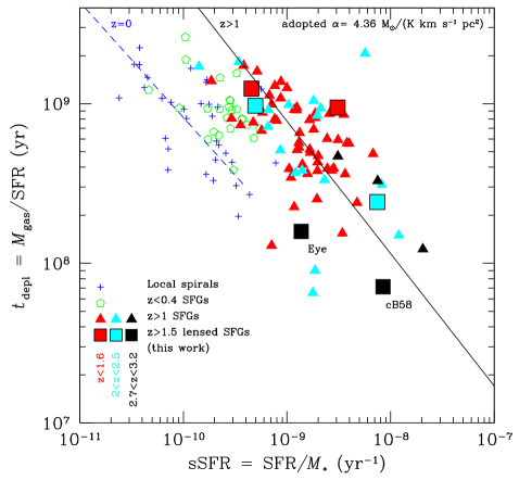
Figure 8: Molecular gas depletion timescales, $t_{\rm depl}=M_{\rm gas}/{\rm SFR}$, as a function of specific star formation rates, ${\rm sSFR=SFR}/M_{*}$, plotted for our low-$L_{\rm IR}$ selected SFGs (squares) and our comparison sample of SFGs and local spirals with CO measurements from the literature (see Sect. 2.2). The molecular gas depletion timescales are computed assuming a “Galactic” CO–H₂ conversion factor for all galaxies. $t_{\rm depl}$ shows a strong dependence on sSFR. The best-fitting bisector linear relation to the $z=0$ COLD GASS sample from Saintonge et al. (2011) is plotted as a dashed blue line. $z>1$ SFGs are displaced with respect to the local relation, their best-fitting bisector linear relation, $\log(t_{\rm depl})=(-0.83\pm 0.08)\log({\rm sSFR})+(1.43\pm 0.70)$, is plotted as a solid black line. The color-coding of SFGs (our sample plus $z>1$ SFGs from the literature) refers to three redshift intervals: $\langle z_{1.2}\rangle=[1,1.6]$ (red), $\langle z_{2.2}\rangle=[2,2.5]$ (cyan), and $\langle z_{3.0}\rangle=[2.7,3.2]$ (black).

5.2.1 Specific star formation rate

A possible physical parameter which may control the SFE or $t_{\rm depl}$ of galaxies is the specific star formation rate, ${\rm sSFR=SFR}/M_{*}$, i.e. the SFR normalized by the stellar mass which gives the timescale of formation of all the stellar mass in a galaxy at the given present SFR. In their study of $z=0$ massive star-forming galaxies with $10.0<\log(M_{*}/{\rm M_{\sun}})<11.5$ from the COLD GASS survey, Saintonge et al. (2011) found the strongest dependence of $t_{\rm depl}$ to be precisely on the sSFR. Their $t_{\rm depl}$–sSFR anti-correlation in fact highlights comparable timescales for the gas consumption and the stellar mass formation. They interpret it as the result of the increased dynamical stirring as one proceeds to more strongly star-forming galaxies, since in local starburst galaxies the very high values of sSFR are achieved because dynamical disturbances act to compress the available interstellar medium atomic gas and create giant molecular clouds and stars.

We also find a good anti-correlation between $t_{\rm depl}$ and sSFR for $z>1$ SFGs as shown in Fig. 8. We overplot the best-fit relation obtained for the COLD GASS sample and observe that $z>1$ SFGs are generally distributed above the $z=0$ relation and have longer $t_{\rm depl}$ by about 0.75 dex than local galaxies with the same sSFR (see the best-fitting relation obtained for $z>1$ SFGs). The observed $t_{\rm depl}$–sSFR anti-correlation and its shift with redshift are in agreement with the “bathtub” model predictions (Bouché et al. 2010) and confirm the findings by Saintonge et al. (2011) and Combes et al. (2013). They attribute this displacement of $z=1-3$ star-forming galaxies with respect to the local galaxy population to their significantly larger molecular gas fractions that afford longer molecular gas depletion times at a given value of sSFR. We do confirm in Sect. 6 the increased available molecular gas reservoir as one proceeds toward higher redshifts, as well as, on average, as one proceeds toward more strongly star-forming galaxies (higher sSFR), which certainly triggers the $t_{\rm depl}$–sSFR anti-correlation observed at $z>1$. Nevertheless, while a clear evolution of the $t_{\rm depl}$-sSFR relation appears to be present between local and $z>1$ galaxies, no clear trend seems to emerge between the three redshift bins $\langle z_{1.2}\rangle=[1,1.6]$, $\langle z_{2.2}\rangle=[2,2.5]$, and $\langle z_{3.0}\rangle=[2.7,3.2]$. This agrees with the steep increase of the molecular gas fraction between $z=0$ and $z\sim 1$ followed by a quasi non-evolution toward higher redshifts (but with a large scatter) as observed in Fig. 13.

In addition to the shift of $z>1$ SFGs with respect to local galaxies due to their larger molecular gas fractions, the specific star formation rates of galaxies in the local Universe are sealed on low values because of the accumulation of more and more old stars in their bulge at $z=0$. These old stars have an important weight in the total stellar mass budget, but none on the current SFR and thus imply low sSFR values. As a result, this accentuates the displacement between the respective distributions of local and high-redshift galaxies in the $t_{\rm depl}$–sSFR plane.

5.2.2 Stellar mass

Another physical parameter which may trigger differences in SFE or $t_{\rm depl}$ from galaxy to galaxy is the stellar mass. In their analysis of $z=0$ massive star-forming galaxies from the COLD GASS survey, Saintonge et al. (2011) could observe an increase in $t_{\rm depl}$ by a factor of 6 over the stellar mass range of $10^{10}\leavevmode\nobreak\ \rm M_{\sun}$ to $10^{11.5}\leavevmode\nobreak\ \rm M_{\sun}$, from about 0.7 Gyr to 4 Gyr. They assign this $t_{\rm depl}$–$M_{*}$ correlation to the more bursty star formation history of low-mass galaxies which leads to enhanced SFE, inversely reduced $t_{\rm depl}$, due to minor starburst events produced either by weak mergers associated with distant tidal encounters, variations in the intergalactic medium accretion rate, or secular processes within galactic disks. On the other hand, morphological quenching and feedback in high-mass galaxies prevent the molecular gas from forming stars, while at the same time not destroying the gas leads to an increased reservoir of molecular gas. This dependence of $t_{\rm depl}$ on $M_{*}$ in local SFGs has been recently confirmed over the full stellar mass range down to $M_{*}=10^{9}\leavevmode\nobreak\ \rm M_{\sun}$ by the ALLSMOG survey from Bothwell et al. (2014).

The increase of the molecular gas depletion timescale with the stellar mass is also observed in our compilation of $z>1$ SFGs with CO measurements from the literature, including our low-$L_{\rm IR}$ selected SFGs, as shown in Fig. 9. It is confirmed with a Kendall’s tau probability of 0.0017 per cent and a slope $M_{*}^{0.5}$. On average, $z>1$ SFGs have shorter $t_{\rm depl}$ than local galaxies with the same $M_{*}$. This $t_{\rm depl}$–$M_{*}$ correlation in order to be compatible with the $t_{\rm depl}$–sSFR anti-correlation discussed above (Sect. 5.2.1), implies that a galaxy at $z>1$ with a given $M_{*}$ necessarily has its SFR higher than a galaxy at $z=0$ with the same $M_{*}$. This is in line with the SFR–$M_{*}$ MS relation (see Fig. 2).

The increase in $t_{\rm depl}$ by a factor of 10 over the stellar mass range of $10^{9.4}\leavevmode\nobreak\ \rm M_{\sun}$ to $10^{11.5}\leavevmode\nobreak\ \rm M_{\sun}$, from about 0.15 Gyr to 1.5 Gyr, we observe in our sample of $z>1$ SFGs, questions the constant $t_{\rm depl}$ of 0.7 Gyr found by Tacconi et al. (2013) in their sample of $z=1-3$ SFGs with stellar masses confined to $M_{*}>10^{10.4}\leavevmode\nobreak\ \rm M_{\sun}$. In Fig. 9, we may see that the $t_{\rm depl}$–$M_{*}$ correlation at high redshift is triggered by galaxies with small stellar masses. This resembles the first $z=0$ surveys that were unable to highlight the $t_{\rm depl}$ correlation with $M_{*}$ because of their limited dynamical range in $M_{*}$. Indeed, in the smaller range of galaxies explored in the THINGS sample, Bigiel et al. (2008) and Leroy et al. (2008) initially found a constant molecular gas depletion timescale.

If true, such a correlation between $t_{\rm depl}$ and $M_{*}$ observed both in local and $z>1$ SFGs has two important implications. First, it is in contradiction with cosmological hydrodynamic simulations by Davé et al. (2011) which predict the opposite, namely an anti-correlation between $M_{*}$ and $t_{\rm depl}$, where $t_{\rm depl}$ drops to larger stellar masses roughly as $M_{*}^{-0.3}$ . Second, it refutes the linearity of the Kennicutt-Schmidt relation, i.e. the proportionality of SFR and molecular gas mass, such that $\Sigma_{\rm SFR}\propto\Sigma_{\rm gas}^{N}$ with $N\neq 1$. This is fundamental, as it contradicts one of the hypotheses of the “bathtub” model that assumes a constant molecular gas depletion timescale, and hence a linear Kennicutt-Schmidt relation (e.g., Bouché et al. 2010; Lilly et al. 2013; Dekel & Mandelker 2014). Therefore, we may wonder whether the $t_{\rm depl}$–$M_{*}$ correlation really exists, or whether we simply see a constant $t_{\rm depl}$ embedded in a very large spread. Only getting more molecular gas depletion timescale measurements for $z>1$ galaxies with small stellar masses will bring a definitive answer.

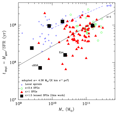
Figure 9: Molecular gas depletion timescales, $t_{\rm depl}=M_{\rm gas}/{\rm SFR}$, as a function of stellar masses plotted for our low-$L_{\rm IR}$ selected SFGs (squares) and our comparison sample of SFGs and local spirals with CO measurements from the literature (see Sect. 2.2). The molecular gas depletion timescales are computed assuming a “Galactic” CO–H₂ conversion factor for all galaxies. A $t_{\rm depl}$–$M_{*}$ correlation emerges for $z>1$ SFGs; their best-fitting bisector linear relation, $\log(t_{\rm depl})=(0.52\pm 0.16)\log(M_{*})+(3.25\pm 1.74)$, is plotted as a solid black line. The best-fitting bisector linear relation to the $z=0$ COLD GASS sample from Saintonge et al. (2011) is shown by the dashed blue line.

A way to reconcile the current empirical finding with a constant $t_{\rm depl}$ is to invoke the possible CO–H₂ conversion factor dependence on metallicity (e.g., Isreal 1997; Leroy et al. 2011; Feldmann et al. 2012; Genzel et al. 2012). Indeed, it is expected that galaxies with lower stellar masses have lower metallicities, according to the mass-metallicity relation (see Sect. 1), and would hence require higher CO–H₂ conversion factors to be applied that would, in reality, lead to longer molecular gas depletion timescales in low stellar mass galaxies in comparison to what we get when assuming a “Galactic” CO–H₂ conversion factor. However, whether this is sufficient to compensate the $t_{\rm depl}$ dependence on $M_{*}^{0.6}$ needs to be further tested.

5.2.3 Redshift

Since the star-forming galaxies span a large interval of the Hubble time, the redshift could also be at the origin of their large SFE or $t_{\rm depl}$ dispersion. Models do predict a cosmic evolution of the molecular gas depletion timescale for main-sequence galaxies (e.g., Hopkins & Beacom 2006; Davé et al. 2011, 2012). The temporal scaling of $t_{\rm depl}$ can be most easily understood when using the formulation of the star formation relation given by ${\rm SFR}\propto M_{\rm gas}/t_{\rm dyn}$, where $t_{\rm dyn}$ is the dynamical time of the star formation region (see also Bouché et al. 2010; Genel et al. 2010). This then gives $t_{\rm depl}\propto t_{\rm dyn}$, which in a canonical disk model scales as $(1+z)^{-1.5}$ (Mo et al. 1998).

The decrease in $t_{\rm depl}$ with redshift is supported by observations, as already reported by Combes et al. (2013), Tacconi et al. (2013), Saintonge et al. (2013), and Santini et al. (2014). In Fig. 10 we plot the molecular gas depletion timescale as a function of redshift for our compilation of local spirals and SFGs with CO measurements from the literature, including our low-$L_{\rm IR}$ selected SFGs. Four redshift bins are considered $\langle z_{0.2}\rangle=[0.055,0.4]$, $\langle z_{1.2}\rangle=[1,1.6]$, $\langle z_{2.2}\rangle=[2,2.5]$, and $\langle z_{3.0}\rangle=[2.7,3.2]$, their respective mean values are $\langle\log(t_{\rm depl}^{\langle z_{0.2}\rangle})\rangle=8.94\pm 0.18$ (870 Myr), $\langle\log(t_{\rm depl}^{\langle z_{1.2}\rangle})\rangle=8.79\pm 0.25$ (620 Myr), $\langle\log(t_{\rm depl}^{\langle z_{2.2}\rangle})\rangle=8.72\pm 0.43$ (520 Myr), and $\langle\log(t_{\rm depl}^{\langle z_{3.0}\rangle})\rangle=8.27\pm 0.33$ (190 Myr) for a “Galactic” CO–H₂ conversion factor. This confirms a shallow $t_{\rm depl}$ decrease from $z=0$ to $z=3.2$, in agreement with the expected $(1+z)^{-1.5}$ dependence. As a result, high redshift SFGs do form stars with a much higher SFE, and consume the molecular gas over a much shorter timescale, than local SFGs. The $t_{\rm depl}$ spread and dispersion per redshift bin are significant, they result from the $t_{\rm depl}$–sSFR and $t_{\rm depl}$–$M_{*}$ relations discussed above (Sects. 5.2.1 and 5.2.2). Indeed, these relations induce a gradient in $t_{\rm depl}$ per redshift bin, such that galaxies with the higher sSFR and smaller $M_{*}$ have the shorter $t_{\rm depl}$.

5.2.4 Offset from the main-sequence

A positive empirical correlation between SFE and the offset from the main-sequence, $\rm sSFR/sSFR_{MS}$, was found by Magdis et al. (2012b), Saintonge et al. (2012), and Sargent et al. (2014), suggesting higher SFE for galaxies with enhanced sSFR and, in particular, for galaxies with $\rm sSFR/sSFR_{MS}\gg 3$, namely beyond the accepted MS thickness, and this independent of galaxies’ redshift. In Fig. 11 we show the SFE of our low-$L_{\rm IR}$ selected galaxies and $z>1$ SFGs from the literature (Sect. 2.2) as a function of their offset from the MS. The main-sequence, ${\rm SFR_{MS}}(z,M_{*})$, is defined here by Eq. (2.1) and is computed at three redshifts covering three redshift intervals $\langle z_{1.2}\rangle=[1,1.6]$, $\langle z_{2.2}\rangle=[2,2.5]$, and $\langle z_{3.0}\rangle=[2.7,3.2]$ of the SFGs. While the enlarged sample of $z>1$ SFGs confirms the general trend of higher SFE for galaxies with larger offsets from the MS (Kendall’s tau probability of 0.025 per cent), the MS galaxies themselves, with offsets from the MS restricted to $0.3<\rm sSFR/sSFR_{MS}<3$ (80% of the sample), have roughly a constant SFE given the Kendall’s tau probability of 0.23 per cent with a large dispersion of 0.32 dex, reaching SFE values even higher than those of galaxies beyond the accepted MS thickness. Consequently, the large spread in SFE observed among MS galaxies over 1.7 orders of magnitude cannot be attributed to the thickness of the SFR–$M_{*}$ relation, i.e. the relative position of galaxies with respect to the main-sequence.

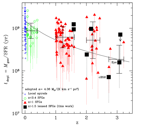
Figure 10: Molecular gas depletion timescales, $t_{\rm depl}=M_{\rm gas}/{\rm SFR}$, as a function of redshift plotted for our low-$L_{\rm IR}$ selected SFGs (squares) and our comparison sample of SFGs and local spirals with CO measurements from the literature (see Sect. 2.2). The molecular gas depletion timescales are computed assuming a “Galactic” CO–H₂ conversion factor for all galaxies, but for $z<0.4$ and $z>1$ SFGs (pentagons, triangles, and squares) the dotted lines, in addition, show the interval of possible $t_{\rm depl}$ values as determined with two extreme CO–H₂ conversion factors $\alpha=4.36$ (“Galactic” value) and 1.1 (local ULIRG value). A redshift evolution of $t_{\rm depl}$ is observed in agreement with the expected $1.5\times(1+z)^{-1.5}$ dependence of Davé et al. (2012), where the normalization is set to the typical depletion time of 1.5 Gyr observed in local galaxies (solid line). Four redshift bins are considered, $\langle z_{0.2}\rangle=[0.055,0.4]$, $\langle z_{1.2}\rangle=[1,1.6]$, $\langle z_{2.2}\rangle=[2,2.5]$, and $\langle z_{3.0}\rangle=[2.7,3.2]$, for the $t_{\rm depl}$ means shown by the large black crosses with their $1\,\sigma$ dispersion.

Saying things on the other way, these results tell us that it is not the star formation efficiency of MS galaxies that drives the thickness of the SFR–$M_{*}$ relation, although the SFE certainly contributes to it in some way within its large spread. What physical parameter then dominates and triggers this thickness ? In Fig. 12 we show that the strongest dependence of the offset from the MS is observed on $M_{\rm gas}/M_{*}$, the molecular gas mass over the stellar mass ratio, with a Kendall’s tau probability of 0 per cent and this over two orders of magnitude. This confirms the findings by Magdis et al. (2012b) and Sargent et al. (2014), who support that the thickness of the SFR–$M_{*}$ relation at any redshift is driven by the variations of the molecular gas fractions of MS galaxies rather than by variations of their star formation efficiencies. According to Magdis et al. (2012b), this prevalence of $M_{\rm gas}/M_{*}$ implies that MS galaxies can have higher SFR (within the thickness of the MS) mainly because they have more raw molecular gas material to produce stars, which hence favours the existence of a global star-formation relation $L_{\rm IR}$(or SFR)–$M_{\rm gas}$ for all MS galaxies (see Fig. 6).

5.2.5 Compactness of the starburst

Downes & Solomon (1998) were the first to point out that the compactness of the nuclear starburst regions was linked to the star formation efficiency in extreme local ULIRGs. Combes et al. (2013) found, in this sense, a weak trend for SFE to be anti-correlated with the half-light radii of high-redshift galaxies, $R_{1/2}$, or correlated with their compactness. The five SFGs with the highest SFE from our compilation of $z>1$ SFGs, including our low-$L_{\rm IR}$ selected galaxies, have $R_{1/2}$ ranging between 1.5 and 4 kpc with one object having $R_{1/2}$ as large as 8 kpc. These half-light radii are typical of high-redshift star-forming galaxies (Tacconi et al. 2013), and thus do not highlight a particular compactness among SFGs with the highest SFE. Certainly, we have to increase the number of available data, in parallel with the angular resolution of CO measurements to confirm or affirm the role of the starburst’s compactness in the SFE (or $t_{\rm depl}$) spread.

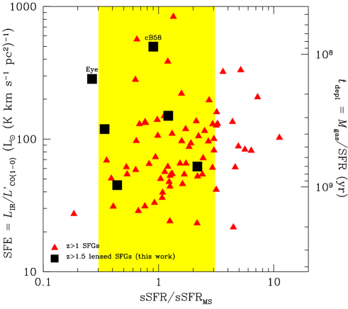
Figure 11: Star formation efficiencies, ${\rm SFE}=L_{\rm IR}/L^{\prime}_{\rm CO(1-0)}$ (left y-axis), or molecular gas depletion timescales, $t_{\rm depl}={\rm SFR}/M_{\rm gas}$, assuming a “Galactic” CO–H₂ conversion factor for all galaxies (right y-axis), as a function of galaxies’ offsets from the main-sequence, $\rm sSFR/sSFR_{MS}$, plotted for our low-$L_{\rm IR}$ selected SFGs (squares) and our comparison sample of $z>1$ SFGs with CO measurements from the literature (triangles). The shaded area defines the accepted thickness of the MS, i.e. a scatter about the SFR–$M_{*}$ relation between $\rm 0.3<sSFR/sSFR_{MS}<3$. The enlarged sample of $z>1$ SFGs confirms the general trend of higher SFE for galaxies with larger offsets from the MS with a Kendall’s tau probability of 0.025 per cent. However, considering MS galaxies only within the shaded area, their SFE appear roughly constant, given the Kendall’s tau probability of 0.23 per cent with a large dispersion of 0.32 dex.

5.2.6 Summary

The answer to the question “what determines the behaviour of the star formation efficiency and molecular gas depletion timescale in star-forming galaxies at high redshift” is not straightforward from what we have discussed above. The dependence of SFE (or $t_{\rm depl}$) on five physical parameters has been investigated. While the dependence appears to be the strongest on the specific star formation rate, there is, in addition, a trend for a correlation with the stellar mass and a clear evolution with redshift. The dependences on the offset from the main-sequence and the compactness of the starburst are less clear. Consequently, there is a tight interplay between the SFE (or $t_{\rm depl}$) and, respectively, the specific star formation rate, the stellar mass, and the redshift of galaxies, which implies that not only one single physical parameter drives the observed large spread in SFE of $z>1$ SFGs, but a combination of all of them.

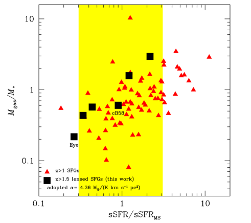
Figure 12: Molecular gas mass over stellar mass ratios, $M_{\rm gas}/M_{*}$, as a function of galaxies’ offsets from the main-sequence, $\rm sSFR/sSFR_{MS}$, plotted for our low-$L_{\rm IR}$ selected SFGs (squares) and our comparison sample of $z>1$ SFGs with CO measurements from the literature (triangles). The shaded area defines the accepted thickness of the MS as above. A clear correlation is observed with a Kendall’s tau probability of 0 per cent.

In addition, an intrinsic spread in SFE and $t_{\rm depl}$ certainly exists due to other, more complex, and hence more difficult to test, effects. For example, some galaxies very likely are not in a quasi-steady state equilibrium, because the accretion rate is not constant, in contrast to what is assumed in the ideal “bathtub” model where the accretion rate and the star formation rate timescale are supposed to vary slowly enough. And obviously, environment and mergers, as well as other variability effects, like an episodic star formation, probably imply a not so smooth galaxy evolution.

6 Molecular gas fraction of high-redshift galaxies

The molecular gas fraction, defined as $f_{\rm gas}=M_{\rm gas}/(M_{\rm gas}+M_{*})$, is a very important physical quantity to know, but also very difficult to access, since dependent on the CO–H₂ conversion factor. We can also express the molecular gas fraction as:

$$f_{\rm gas}=\frac{1}{1+(t_{\rm depl}{\rm sSFR})^{-1}}\,,$$ (2)

meaning that it is closely linked to the molecular gas depletion timescale and the specific star formation rate. Observations show a clear trend of increasing $f_{\rm gas}$ with sSFR (Tacconi et al. 2013), but with a large dispersion (larger than the systematic uncertainties in sSFR and $f_{\rm gas}$ measurements) induced by the different molecular gas depletion timescales found among $z>1$ SFGs, ranging between 0.15 Gyr and 1.5 Gyr (see Sect. 5.2).

The various physical processes at play in the evolution of galaxies (e.g., accretion, star formation, and feedback) have direct impact on the behaviour of their molecular gas fraction. Consequently, a solid way to test galaxy evolution models is to confront their predictions with the observed $f_{\rm gas}$ behaviour. We consider below two main observables, the redshift and the stellar mass, and investigate the respective redshift evolution and stellar mass dependence of $f_{\rm gas}$ in high-redshift SFGs.

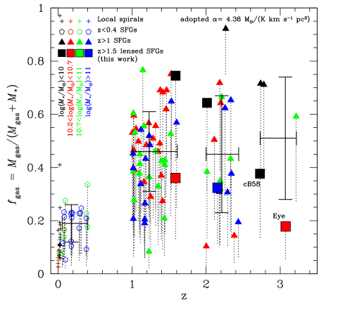
Figure 13: Molecular gas fractions, $f_{\rm gas}=M_{\rm gas}/(M_{\rm gas}+M_{*})$, as a function of redshift plotted for our low-$L_{\rm IR}$ selected SFGs (squares) and our comparison sample of SFGs and local spirals with CO measurements from the literature (see Sect. 2.2). The molecular gas fractions are computed assuming a “Galactic” CO–H₂ conversion factor for all galaxies, but for $z<0.4$ and $z>1$ SFGs (pentagons, triangles, and squares) the dotted lines, in addition, show the interval of possible $f_{\rm gas}$ values as determined with two extreme CO–H₂ conversion factors $\alpha=4.36$ (“Galactic” value) and 1.1 (local ULIRG value). Four redshift bins are considered, $\langle z_{0.2}\rangle=[0.055,0.4]$, $\langle z_{1.2}\rangle=[1,1.6]$, $\langle z_{2.2}\rangle=[2,2.5]$, and $\langle z_{3.0}\rangle=[2.7,3.2]$, for the $f_{\rm gas}$ means shown by the large black crosses with their $1\,\sigma$ dispersion. A net rise of $f_{\rm gas}$ is observed from $\langle z_{0.2}\rangle$ to $\langle z_{1.2}\rangle$, followed by a very mild increase toward higher redshifts. The color-coding refers to four stellar mass intervals: $\log(M_{*}/{\rm M}_{\sun})<10$ (black), $10.2<\log(M_{*}/{\rm M}_{\sun})<10.7$ (red), $10.7<\log(M_{*}/{\rm M}_{\sun})<11$ (green), and $\log(M_{*}/{\rm M}_{\sun})>11$ (blue), as defined in Sect. 6.2.

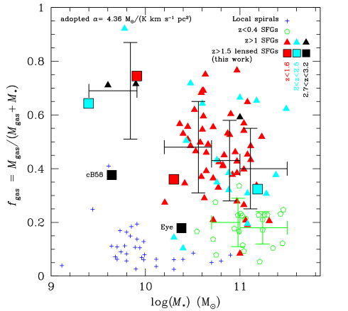
Figure 14: Molecular gas fractions, $f_{\rm gas}=M_{\rm gas}/(M_{\rm gas}+M_{*})$, as a function of stellar masses plotted for our low-$L_{\rm IR}$ selected SFGs (squares) and our comparison sample of SFGs and local spirals with CO measurements from the literature (see Sect. 2.2). The molecular gas fractions are computed assuming a “Galactic” CO–H₂ conversion factor for all galaxies. Four stellar mass bins are considered $9.4<\log(M_{*}/{\rm M_{\sun}})<9.9$, $10.2<\log(M_{*}/{\rm M_{\sun}})<10.7$, $10.7<\log(M_{*}/{\rm M_{\sun}})<11.0$, and $11.0<\log(M_{*}/{\rm M_{\sun}})<11.5$. The corresponding $f_{\rm gas}$ means with their $1\,\sigma$ dispersion of $z>1$ SFGs are shown by the large black crosses and of $z<0.4$ SFGs by the large green crosses. The $M_{*}$ dependence of $f_{\rm gas}$ sustains an upturn of the molecular gas fraction at the low-$M_{*}$ end, a mild decrease toward higher stellar masses of SFGs at $z>1$, and a shift toward lower $f_{\rm gas}$ values for SFGs at lower redshifts. The color-coding of SFGs (our sample plus $z>1$ SFGs from the literature) refers to three redshift intervals: $\langle z_{1.2}\rangle=[1,1.6]$ (red), $\langle z_{2.2}\rangle=[2,2.5]$ (cyan), and $\langle z_{3.0}\rangle=[2.7,3.2]$ (black).

6.1 Redshift evolution of the molecular gas fraction

The cosmic evolution of the molecular gas fraction with the Hubble time directly results from the expansion of the Universe itself. New matter falling on galaxies through accretion from filaments comes from further out as the time progresses and, consequently, high angular momentum matter settles in the outer parts of galaxies. This leads to the size growth of galaxies with the cosmic time, such that galaxies were more compact in the early Universe than today. A finding first proposed by dark matter simulations (e.g., Fall & Efstathiou 1980; Mo et al. 1998), more recently by cosmological hydrodynamic simulations including cold gas accretion (Stewart et al. 2013), and now observationally confirmed (e.g., Bouwens et al. 2004; Trujillo et al. 2006; Buitrago et al. 2008). The size growth of galaxies has a direct impact on the H₂/H I ratio evolution. Indeed, the pressure on the midplane of galaxies strongly depends on the gas surface density, in the way that a smaller radius increases the gas surface density. Since the H₂/H I ratio is strongly correlated to this pressure, for the same gas mass the high-redshift galaxies, which are smaller (more compact) and hence have a higher internal pressure, will have a higher H₂/H I ratio and that means a higher H₂ content than local galaxies (e.g., Obreschkow & Rawlings 2009; Lagos et al. 2011, 2014). This together with the trend for high-redshift galaxies to be intrinsically more gas-rich, i.e. have a higher total gas mass ($\rm H\,I+H_{2}$), leads to even larger difference between high-redshift and local galaxies and hence to a net increase of the molecular gas fraction with redshift.

From Eq. (2) we see that the evolution of the molecular gas fraction depends on the evolution of both $t_{\rm depl}$ and sSFR. We have shown in Sect. 5.2.3 that the molecular gas depletion timescale evolves with $(1+z)^{-1.5}$. The “bathtub” model, in parallel, predicts a continuing rise of the specific star formation rate, generally driven by the redshift evolution of the average accretion rate (inflow), which scales as $(1+z)^{\alpha}$ with $\alpha$ varying between 5/3 and 3 according to the prescriptions considered (Bouché et al. 2010; Davé et al. 2012; Lilly et al. 2013). The steeper rise of the specific star formation rate with respect to the decline of the molecular gas depletion timescale leads to the steady increase of $f_{\rm gas}$ with redshift.

Observationally, the cosmic evolution of the molecular gas fraction with the Hubble time, in the way that higher redshift galaxies are more gas-rich, is now well established (e.g., Daddi et al. 2010a; Geach et al. 2011; Tacconi et al. 2010, 2013; Saintonge et al. 2013; Sargent et al. 2014; Carilli & Walter 2013). In Fig. 13 we show $f_{\rm gas}$ as a function of redshift for our compilation of local spirals and SFGs with CO measurements from the literature, including our low-$L_{\rm IR}$ selected SFGs. We consider four redshift bins $\langle z_{0.2}\rangle=[0.055,0.4]$, $\langle z_{1.2}\rangle=[1,1.6]$, $\langle z_{2.2}\rangle=[2,2.5]$, and $\langle z_{3.0}\rangle=[2.7,3.2]$. The respective mean values $\langle f_{\rm gas}^{\langle z_{0.2}\rangle}\rangle=0.19\pm 0.07$, $\langle f_{\rm gas}^{\langle z_{1.2}\rangle}\rangle=0.46\pm 0.15$, $\langle f_{\rm gas}^{\langle z_{2.2}\rangle}\rangle=0.45\pm 0.22$, and $\langle f_{\rm gas}^{\langle z_{3.0}\rangle}\rangle=0.51\pm 0.23$ for a “Galactic” CO–H₂ conversion factor show a net rise of the molecular gas fraction from $\langle z_{0.2}\rangle$ to $\langle z_{1.2}\rangle$, followed by a very mild increase toward higher redshifts, as found in earlier studies. If further confirmed, such an $f_{\rm gas}$ redshift evolution does not really correspond to a steady redshift increase of $f_{\rm gas}$ as predicted by the “bathtub” model. It requires a different redshift-dependence of either $t_{\rm depl}$ or sSFR (see Eq. (2)). The sSFR redshift evolution parametrised by Lilly et al. (2013) proposes a steep sSFR increase as $(1+z)^{3}$ out to $z=2$ and a slow down to $(1+z)^{5/3}$ at $z>2$. This model is among the closest to the observations, since it predicts a flattening of the $f_{\rm gas}$ evolution beyond $z=2$ (see also Saintonge et al. 2013).

The spread and dispersion of the molecular gas fractions per redshift bin are significant, in particular for $z>1$ SFGs. As discussed in Carilli & Walter (2013), a large $f_{\rm gas}$ dispersion at a given redshift is expected: it is mainly due to the strong dependence of $f_{\rm gas}$ on the stellar mass (shown in Sect. 6.2), which should produce an $f_{\rm gas}$ gradient per redshift bin, such that galaxies with the smaller $M_{*}$ have the larger $f_{\rm gas}$ (see Fig. 14). To highlight the effect of this dependence, the color-coding of the data points in Fig. 13 refers to four stellar mass bins. We may see that the data points within the lowest $M_{*}$ bin ($\log(M_{*}/{\rm M}_{\sun})<10$) do show the larger $f_{\rm gas}$ per redshift bin. The expected $f_{\rm gas}$ gradient with $M_{*}$ per redshift bin for galaxies within the other $M_{*}$ bins is more scattered, but we still see its effect on the $z<0.4$ SFGs which have the smallest dispersion because they cover the two higher $M_{*}$ bins only. The stellar mass is not the only physical parameter inducing an $f_{\rm gas}$ dispersion per redshift bin. The star formation rate plays an important role too, since $f_{\rm gas}$ increases with SFR as a consequence of the Kennicutt-Schmidt relation (see the fundamental $f_{\rm gas}$–$M_{*}$–SFR relation proposed by Santini et al. (2014)), as well as environmental effects (outflows, disk hydrostatic pressure, etc.).

6.2 Stellar mass dependence of the molecular gas fraction

Bouché et al. (2010), Davé et al. (2011), and Lagos et al. (2014), all show a drop in the molecular gas fraction with increasing stellar mass and an upturn of $f_{\rm gas}$ at the low-$M_{*}$ end. The location and strength of that upturn depends on the model adopted and, in particular, on whether any outflow is considered. A comparable $M_{*}$ dependence of the molecular gas fraction is predicted for both local and high-redshift galaxies, but with a shift in $f_{\rm gas}$ toward higher values at higher redshifts, a shift that results from the redshift evolution of $f_{\rm gas}$ (see Fig. 13). While in a closed-box model the molecular gas fraction is expected to decrease with the stellar mass because of the gas conversion into stars, this turns out to be similar in the “bathtub” model as the modelled galaxies approach a steady state where the SFR, which is proportional to the gas mass, represents the rate at which gas is turned into stars, follows the net gas accretion rate dictated by cosmology plus a gas outflow rate (Dekel & Mandelker 2014).

The $M_{*}$ dependence of $f_{\rm gas}$ at $z>1$ has already been observationally constrained by Tacconi et al. (2013) and Santini et al. (2014) for galaxies at the intermediate/high-$M_{*}$ end $10.4<\log(M_{*}/{\rm M}_{\sun})<12$ (see also Magdis et al. 2012b; Sargent et al. 2014). We provide for the first time insights on $f_{\rm gas}$ of high-redshift SFGs at the low-$M_{*}$ end $9.4<\log(M_{*}/{\rm M}_{\sun})<9.9$. Our new sample of low-$L_{\rm IR}$ selected SFGs doubles the number of galaxies at $z>1$ (3 out of a total of 6) with achieved $f_{\rm gas}$ measurements at the low-$M_{*}$ end. In Fig. 14 we show the resulting $f_{\rm gas}$ as a function of stellar mass. We divide the sample of $z>1$ SFGs with intermediate/high-$M_{*}$ in three stellar mass bins $10.2<\log(M_{*}/{\rm M_{\sun}})<10.7$, $10.7<\log(M_{*}/{\rm M_{\sun}})<11.0$, and $11.0<\log(M_{*}/{\rm M_{\sun}})<11.5$, each containing a comparable number of galaxies. The respective mean values $\langle f_{\rm gas}^{\langle M_{*\,10.5}\rangle}\rangle=0.48\pm 0.17$, $\langle f_{\rm gas}^{\langle M_{*\,10.9}\rangle}\rangle=0.43\pm 0.15$, and $\langle f_{\rm gas}^{\langle M_{*\,11.1}\rangle}\rangle=0.40\pm 0.15$ for a “Galactic” CO–H₂ conversion factor show a mild decrease of $f_{\rm gas}$ with stellar mass within a very large dispersion. On the other hand, the mean $\langle f_{\rm gas}^{\langle M_{*\,{9.7}}\rangle}\rangle=0.69\pm 0.18$ value of the lowest stellar mass bin $9.4<\log(M_{*}/{\rm M}_{\sun})<9.9$ highlights an upturn of $f_{\rm gas}$ at the low-$M_{*}$ end of SFGs at $z>1$ as predicted. More data in the low-$M_{*}$ end, tackling the $f_{\rm gas}$ upturn, may help disentangling specific outflow/feedback/wind recipes.

The mean values of $f_{\rm gas}$ within the two higher stellar mass bins defined above were also computed for SFGs at $z<0.4$ and are plotted in Fig. 14. They nicely show the shift of the $M_{*}$ dependence toward smaller molecular gas fractions that is expected for star-forming galaxies at lower redshifts, because of the redshift evolution of $f_{\rm gas}$ (Sect. 6.1). This evolution is also partly responsible for the large dispersion observed within each $M_{*}$ bin of $z>1$ SFGs, as shown by the color-coding of the data points of $z>1$ SFGs highlighting three redshift bins.

The combination of the redshift evolution and $M_{*}$ dependence of the molecular gas fraction shows not only that the average $f_{\rm gas}$ of star-forming galaxies increases with redshift (Sect. 6.1), but that this increase is even more substantial for low stellar mass galaxies than for the high stellar mass ones given the upturn of $f_{\rm gas}$ at the low-$M_{*}$ end for $z>1$ SFGs. A behaviour judged by Bouché et al. (2010) and Santini et al. (2014) as being a direct result of the “downsizing” scenario, which claims that more massive galaxies formed earlier and over a shorter period of time (e.g., Cowie et al. 1996; Heavens et al. 2004; Jimenez et al. 2007; Thomas et al. 2010), i.e., consume their molecular gas more quickly. Consequently, massive galaxies have already consumed most of their gas at high redshifts, while less massive galaxies still have a large fraction of molecular gas.

7 Dust-to-gas ratio

The Herschel/PACS+SPIRE and longer wavelength data of our low-$L_{\rm IR}$ selected SFGs allow accessing their dust masses (see Table 1 and Sklias et al. 2014). When combined with CO emission data, we may hence investigate another key physical parameter that is the dust-to-gas mass ratio, $\delta_{\rm DGR}=M_{\rm dust}/M_{\rm gas}$. This is even more important, as the dust-to-gas mass ratio and dust masses start to be used to estimate the CO–H₂ conversion factor both in local and high-redshift galaxies (e.g., Leroy et al. 2011; Magdis et al. 2011, 2012b; Magnelli et al. 2012) and to determine molecular gas masses when CO measurements are not available (Santini et al. 2014; Scoville et al. 2014).

It is now accepted both from observations and interstellar medium evolution models that $\delta_{\rm DGR}$ scales linearly with the oxygen abundance (e.g., Issa et al. 1990; Dwek 1998; Edmunds 2001; Inoue 2003; Draine et al. 2007; Leroy et al. 2011; Saintonge et al. 2013; Chen et al. 2013). Nevertheless, the measure of the dust-to-gas mass ratio, in particular, in high-redshift galaxies remains very uncertain, because of a number of important assumptions that are done:

1. The dust mass derivation from the far-IR/sub-mm SED is tributary to several assumptions, such as the dust model, the dust emissivity index $\beta$ within the modified black-body (MBB) fits, and the dust mass absorption cross section. The freedom on these parameters can lead to large variations in the $M_{\rm dust}$ estimates. Magnelli et al. (2012) already pointed out a factor of 3 difference between dust masses as inferred from MBB fits and the Draine & Li (2007) model.

2. A CO–H₂ conversion factor needs to be assumed to determine the molecular gas mass. Since the CO–H₂ conversion factor is suspected to vary with metallicity, this could induce a false $\delta_{\rm DGR}$–metallicity dependence.

3. At high redshift we consider $M_{\rm H_{2}}\gg M_{\rm H\,I}$, or equivalently $M_{\rm gas}\approx M_{\rm H_{2}}=M_{\rm dust}/\delta_{\rm DGR}$. This is supported by the high molecular gas fractions measured in $z>1$ SFGs (see Fig. 13), which leave little room for a significant atomic gas component within the total mass budget as inferred from dynamical analysis (Daddi et al. 2010a; Tacconi et al. 2010) and theoretical arguments like those discussed in Sect. 6.1 (e.g., Obreschkow & Rawlings 2009; Lagos et al. 2011, 2014). However, no direct H I measurements exist in high-redshift galaxies so far.

To alleviate the uncertainty on the above first assumption, Scoville et al. (2014) proposed to consider the long-wavelength far-IR/sub-mm continuum as a dust mass tracer, since the long-wavelength Rayleigh-Jeans tail of dust emission is generally optically thin and thus provides a direct probe of the total dust. They chose 850 $\mu$m as the fiducial wavelength and measured, in a homogeneous way, $\delta_{\rm DGR}\approx L_{\nu}(850\,\mu{\rm m})/M_{\rm gas}$ in the Galaxy, local spirals, local ULIRGs, and high-redshift SMGs by assuming for all a spectral slope $\beta=1.8$ for the far-IR/sub-mm dust emission flux density as determined from the extensive Planck data throughout the Galaxy (Planck Collaboration 2011a, b) and a “Galactic” CO–H₂ conversion factor .

Following the Scoville et al. (2014) prescriptions, we add to their sample our low-$L_{\rm IR}$ selected SFGs (see their rest-frame 850 $\mu$m luminosities in Table 1) and the compilation of $z>1$ SFGs with CO measurements from the literature (Sect. 2.2) for which published far-IR/sub-mm photometry is available (Magdis et al. 2012b; Saintonge et al. 2013). In addition, in order to bypass effects linked to the possible dust-to-gas ratio dependence on metallicity, we consider only the star-forming galaxies with near-solar metallicities $Z/Z_{\sun}>0.8$. The metallicities are estimated using the mass–metallicity relation at $z\sim 2.2$ from Erb et al. (2006) recalibrated by Maiolino et al. (2008) and scaled to the Chabrier (2003) IMF, when direct metallicity measurements from nebular emission lines are not available. 12 out of 73 CO-detected SFGs at $z>1$ (including our low-$L_{\rm IR}$ selected SFGs) satisfy the above prescriptions. Similarly to Scoville et al., we adopt the “Galactic” CO–H₂ conversion factor, which in the case of these high-redshift SFGs is reasonable given their near-solar metallicities (and see also Sect. 4). The $L_{\nu}(850\,\mu{\rm m})/M_{\rm gas}$ results of these $z>1$ SFGs are shown in Fig. 15 as a function of $L_{\nu}(850\,\mu{\rm m})$ and are compared to local spirals, local ULIRGs, and high-redshift SMGs from Scoville et al. The respective means and dispersions are:

$$\langle L_{\nu}(850\,\mu{\rm m})/M_{\rm gas}\rangle_{\rm SFGs} = 4.66^{+3.03}_{-1.84}\times 10^{19}\leavevmode\nobreak\ \rm erg\leavevmode\nobreak\ s^{-1}\leavevmode\nobreak\ Hz^{-1}\leavevmode\nobreak\ M_{\sun}^{-1}$$

$$\langle L_{\nu}(850\,\mu{\rm m})/M_{\rm gas}\rangle_{\rm SMGs} = 9.54^{+6.00}_{-3.68}\times 10^{19}\leavevmode\nobreak\ \rm erg\leavevmode\nobreak\ s^{-1}\leavevmode\nobreak\ Hz^{-1}\leavevmode\nobreak\ M_{\sun}^{-1}$$

$$\langle L_{\nu}(850\,\mu{\rm m})/M_{\rm gas}\rangle_{\rm local} = 1.01^{+0.27}_{-0.21}\times 10^{20}\leavevmode\nobreak\ \rm erg\leavevmode\nobreak\ s^{-1}\leavevmode\nobreak\ Hz^{-1}\leavevmode\nobreak\ M_{\sun}^{-1}\,.$$

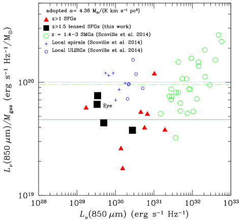
Figure 15: Dust emission at rest-frame 850 $\mu$m per unit mass of gas, $L_{\nu}(850\,\mu{\rm m})/M_{\rm gas}$, plotted for our low-$L_{\rm IR}$ selected SFGs (squares) and our comparison sample of $z>1$ SFGs with CO measurements from the literature and published far-IR/sub-mm photometry (triangles). Only SFGs with metallicities $Z/Z_{\sun}>0.8$ are considered. These results are compared with the compilation from Scoville et al. (2014) for the SMGs at $z=1.4-3$ and local spirals and ULIRGs. We assume a “Galactic” CO–H₂ conversion factor for all objects and $M_{\rm gas}\simeq M_{\rm H_{2}}$ for high-redshift galaxies. All galaxies have a similar $L_{\nu}(850\,\mu{\rm m})/M_{\rm gas}$ within $1-2\,\sigma$, with a trend toward a lower dust-to-gas ratio in $z>1$ SFGs by $\sim 0.33\leavevmode\nobreak\ \rm dex$ at fixed near-solar metallicity, as shown by the lines corresponding, respectively, to the $L_{\nu}(850\,\mu{\rm m})/M_{\rm gas}$ means of local spirals and ULIRGs (blue dotted line), high-redshift SMGs (green dashed line), and $z>1$ SFGs (red solid line).

Measurements in local galaxies (spirals and ULIRGs), $z=1.4-3$ SMGs, and $z>1$ SFGs, at fixed near-solar metallicity ($Z/{\rm Z}_{\sun}>0.8$), show similar $L_{\nu}(850\,\mu{\rm m})/M_{\rm gas}$ means within $1-2\,\sigma$ dispersion. While the means of local galaxies and high-redshift SMGs are nearly the same, $z>1$ SFGs sustain a trend for a shift toward a lower $L_{\nu}(850\,\mu{\rm m})/M_{\rm gas}$ mean by $\sim 0.33\leavevmode\nobreak\ \rm dex$ with a large dispersion of 0.22 dex. Such a shift in $z>1$ SFGs was already reported by Saintonge et al. (2013, by about 0.23 dex) when compared to Local Group galaxies (Leroy et al. 2011). If the dust-to-gas ratio truly is lower in high-redshift SFGs, this may suggest that a smaller fraction of dust grains is produced for the same metallicity under the specific conditions prevailing in the interstellar medium of these galaxies in comparison with local galaxies and high-redshift SMGs.

The data thus support a non-universal $\delta_{\rm DGR}$. Hence, deriving molecular gas masses from direct CO measurements remains highly recommended, as CO still appears a better tracer of the molecular gas mass, despite the uncertainty linked with the CO-to-H₂ conversion factor, than dust.

8 Summary and conclusions

We report new CO observations performed with the IRAM PdBI and 30 m telescope for five strongly-lensed star-forming galaxies at $z\sim 1.5-3$. These galaxies were selected from the Herschel Lensing Survey for their low intrinsic IR luminosities and high magnification factors. Four of them have IR luminosities as low as $L_{\rm IR}<4\times 10^{11}\leavevmode\nobreak\ \rm L_{\sun}$ ($\rm SFR<40\leavevmode\nobreak\ M_{\sun}\leavevmode\nobreak\ yr^{-1}$) and reach the $L^{\star}$ to sub-$L^{\star}$ domain. While this regime is typical of SFGs, the molecular gas content of such galaxies has been poorly explored so far, because of mm/sub-mm instrumental sensitivity limitations. Thanks to the gravitational lensing, we achieve three CO emission detections in $L^{\star}$ to sub-$L^{\star}$ SFGs and a fourth in an SFG with a slightly higher $L_{\rm IR}$. These SFGs not only are among galaxies with the lower $L_{\rm IR}$ with accessible CO luminosities known, but also with the smaller stellar masses $M_{*}<2.5\times 10^{10}\leavevmode\nobreak\ \rm M_{\sun}$. We add to this sample, cB58 and the Eye, two well-known strongly-lensed galaxies characterized by similar low $L_{\rm IR}$ and small $M_{*}$ properties, as derived by Sklias et al. (2014) from revised Herschel photometry and SED fitting. To put these SFGs in the general context of all CO-detected galaxies, we built up a large comparison sample of local and high-redshift galaxies with CO measurements reported in the literature that is exhaustive for high-redshift SFGs, complete for high-redshift SMGs, and only indicative for local spirals, LIRGs, and ULIRGs.

This comparison sample allows us to obtain good estimates of the CO luminosity correction factors r_2,1 and r_3,1 for, respectively, the $J=2$ and $J=3$ CO rotational transitions for both $z=0$ and $z>1$ galaxies distributed over three $L_{\rm IR}$ intervals. Two main trends pop out in agreement with the models of Lagos et al. (2012): (1) shallower CO SLEDs for high-redshift galaxies compared to their $z=0$ counterparts at a fixed IR luminosity, and (2) smaller differences in the CO SLEDs of faint- and bright-IR galaxies at $z>1$ than for $z=0$ galaxies. The inferred means of the observed CO luminosity correction factors valid for SFGs at $z>1$ are r${}_{2,1}=0.81\pm 0.20$ and r${}_{3,1}=0.57\pm 0.15$.

The combination of the overall physical properties derived from the new CO measurements achieved in our SFGs covering a new dynamical range of $\rm SFR<40\leavevmode\nobreak\ \rm M_{\sun}\leavevmode\nobreak\ yr^{-1}$ and $M_{*}<2.5\times 10^{10}\leavevmode\nobreak\ \rm M_{\sun}$ with the comparison sample of CO-detected galaxies from the literature leads to the following main results.

1. A single linear relation within the $L_{\rm IR}$–$L^{\prime}_{\rm CO(1-0)}$ log plane is observed, which best-fit gives a slope of 1.17. The current larger sample of $z>1$ SFGs shows an increased $1\,\sigma$ dispersion of 0.3 dex in the y-direction about the best-fit of their $L_{\rm IR}$–$L^{\prime}_{\rm CO(1-0)}$ relation, which is sufficient to hide the reported bimodal behaviour between the ‘sequence of disks’ and the ‘sequence of starbursts’.

2. Another way to represent the $L_{\rm IR}$–$L^{\prime}_{\rm CO(1-0)}$ relation is through the star formation efficiency, defined as ${\rm SFE}=L_{\rm IR}/L^{\prime}_{\rm CO(1-0)}\equiv{\rm SFR}/M_{\rm gas}=1/t_{\rm depl}$. SFGs and SMGs at $z>1$ show very similar SFE distributions and large spreads; the SFE of $z>1$ SFGs are not confined to the low values of local spirals any more. The investigation of the SFE and $t_{\rm depl}$ dependence on several physical parameters leads us to conclude that it is the combination of the specific star formation rate, stellar mass, and redshift that drives the large spread in SFE of $z>1$ SFGs. The respective offset of SFGs from the main-sequence within the thickness of the SFR–$M_{*}$ relation, as well as the compactness of the starburst seem to play a minor role in the observed SFE spread.

3. The strongest dependence of $t_{\rm depl}$ is observed on the specific star formation rate both for $z>1$ SFGs and local galaxies. SFGs at $z>1$ show longer $t_{\rm depl}$ by about 0.75 dex than local galaxies with the same sSFR. This displacement of the $t_{\rm depl}$–sSFR relation with redshift is attributed to the larger molecular gas fractions found in $z>1$ SFGs that afford longer molecular gas depletion times at a given value of sSFR. In addition, the sSFR of $z=0$ galaxies are sealed on low values, because of the accumulation of more and more old stars in their bulge that have an important weight in the total stellar mass budget, but none on the present SFR.

4. A correlation between the molecular gas depletion timescale and stellar mass is observed thanks to the enlarged dynamical range of stellar masses down to $M_{*}=10^{9.4}\leavevmode\nobreak\ \rm M_{\sun}$ sampled by our low-$L_{\rm IR}$ selected SFGs. Although it needs to be confirmed with additional $z>1$ SFGs with small stellar masses, a $t_{\rm depl}$ increase with $M_{*}$ is seen in $z=0$ galaxies over the $M_{*}$ range from $10^{9}\leavevmode\nobreak\ \rm M_{\sun}$ to $10^{11.5}\leavevmode\nobreak\ \rm M_{\sun}$. If true, this $t_{\rm depl}$–$M_{*}$ correlation observed both in local galaxies and $z>1$ SFGs is opposed to the constant molecular gas depletion timescale assumed in the “bathtub” model and refutes the linearity of the Kennicutt-Schmidt relation.

5. We confirm the $(1+z)^{-1.5}$ evolution of the molecular gas depletion timescale for main-sequence galaxies as predicted by various models. The mean $t_{\rm depl}$ drops from 870 Myr at $\langle z_{0.2}\rangle=[0.055,0.4]$ down to 190 Myr at $\langle z_{3.0}\rangle=[2.7,3.2]$ with a significant dispersion per redshift bin. This dispersion results from the $t_{\rm depl}$–sSFR and $t_{\rm depl}$–$M_{*}$ relations, which induce a gradient of $t_{\rm depl}$ per redshift bin, such that galaxies with the higher sSFR and smaller $M_{*}$ have the shorter $t_{\rm depl}$.

6. Observationally, it is now well established that high-redshift galaxies are gas-rich. What remains debated is the steady increase of the molecular gas reservoir with redshift predicted by models. While we do observe a net rise of the mean $f_{\rm gas}$ from $0.19\pm 0.07$ up to $0.46\pm 0.15$ between $\langle z_{0.2}\rangle=[0.055,0.4]$ and $\langle z_{1.2}\rangle=[1,1.6]$, it is followed by a very mild increase toward higher redshifts. A significant $f_{\rm gas}$ dispersion is seen per redshift bin, it is due to the strong dependence of the molecular gas fraction on the stellar mass, which we start testing observationally.

7. An $f_{\rm gas}$ drop with increasing $M_{*}$ because of the gas conversion into stars, as well as an $f_{\rm gas}$ upturn at the low-$M_{*}$ end whose strength is dependent on the outflow are predicted. $z>1$ SFGs show a mild $f_{\rm gas}$ decrease between $10^{10.4}<M_{*}/{\rm M}_{\sun}<10^{11.5}$. The large dispersion per stellar mass bin comes from the $f_{\rm gas}$ redshift evolution, as nicely illustrated by $z<0.4$ SFGs that have their $M_{*}$ dependence shifted toward lower $f_{\rm gas}$. We provide the first insights on $f_{\rm gas}$ of $z>1$ SFGs at the low-$M_{*}$ end $10^{9.4}<M_{*}/{\rm M}_{\sun}<10^{9.9}$. The corresponding mean $\langle f_{\rm gas}\rangle=0.69\pm 0.18$ value supports an $f_{\rm gas}$ upturn. This shows that the average $f_{\rm gas}$ of SFGs not only increases with redshift, but this increase is even more substantial for low $M_{*}$ galaxies than for the high $M_{*}$ ones, a behaviour resulting from the “downsizing” scenario.

8. To alleviate the uncertainties linked to the dust mass estimates, we consider the rest-frame 850 $\mu$m continuum as a dust mass tracer and compare the dust-to-gas mass ratios, $\delta_{\rm DGR}\approx L_{\nu}(850\,\mu{\rm m})/M_{\rm gas}$, inferred in a homogeneous way, of $z>1$ SFGs to those of local spirals, local ULIRGs, and high-redshift SMGs. While the $L_{\nu}(850\,\mu{\rm m})/M_{\rm gas}$ means of local galaxies and high-redshift SMGs are nearly the same, the one of high-redshift SFGs scatters systematically by a factor of two at fixed near-solar metallicity ($Z/{\rm Z}_{\sun}>0.8$). $z>1$ SFGs sustain a shift toward a lower $L_{\nu}(850\,\mu{\rm m})/M_{\rm gas}$ mean by 0.33 dex with a very large dispersion of 0.22 dex. This supports a non-universal $\delta_{\rm DGR}$. Thus, deriving molecular gas masses from direct CO measurements remains highly recommended.

Appendix A CO properties and kinematics of the individual low-$L_{\rm IR}$ selected galaxies

A.1 A68-C0

The CO(2–1) intensity peak is detected at $11\,\sigma$ in A68-C0, which makes it a very secure CO detection in this $z_{\rm H\alpha}=1.5864$ galaxy, as shown in Figs. 3 and 4. The CO(2–1) emission is well centred on the HST images to within $0.5^{\prime\prime}$. The HST images clearly reveal the presence of two counterpart images of the same galaxy with a morphology typical of a spiral galaxy. The spiral structure is strongly stretched and extended by gravitational lensing, but the two counterpart images that are mirrored are easily identified by the two bright bulges observed north and south with the critical line passing in between. The two counterpart images of this galaxy are not resolved in CO, but they both contribute to the detected CO emission given the CO emission intensity precisely peaking on the critical line and the CO elongation in the direction of the stretch. The two counterpart images are amplified by the same magnification factor.

The CO(2–1) spectrum reveals a double-peaked emission line profile with a total full width half maximum $\rm FWHM_{CO}=334\leavevmode\nobreak\ km\leavevmode\nobreak\ s^{-1}$ and an observed integrated flux $F_{\rm CO}=1.89\pm 0.28\leavevmode\nobreak\ \rm Jy\leavevmode\nobreak\ km\leavevmode\nobreak\ s^{-1}$. The measured CO redshift agrees very well with the H$\alpha$ redshift to within $\Delta z=(z_{\rm H\alpha}-z_{\rm CO})=0.001$. The derived lensing-corrected molecular gas fraction $f_{\rm gas}=0.38$ is much higher than the molecular gas fractions of local spirals, but is comparable to the $f_{\rm gas}$ distribution of SFGs with CO measurements from the literature in the $\langle z_{1.2}\rangle=[1,1.6]$ interval which has a mean $\langle f_{\rm gas}^{\langle z_{1.2}\rangle}\rangle=0.46\pm 0.15$ (see Sect. 6.1).

The observed double-peaked CO emission line profile is a first strong indication of rotation in A68-C0 (Daddi et al. 2010a). Two additional observational facts support rotation in this galaxy. First, its spiral morphology as seen in HST images (see Fig. 3). Second, as shown in Fig. 16 the CO contours integrated over the channels that define the blue-shifted component (blue contours) of the double-peaked CO emission line profile (Fig. 4) appear to be much more extended in comparison to the contours integrated over the channels that define the red-shifted component (red contours) of the CO profile that are more compact. This is a direct consequence of rotation combined with gravitational lensing. Indeed, the critical line is located right in the middle of the two multiple images and is at an angle relative to the major axis of the spiral structure. Because the blue-shifted velocities relative to the observer are the farthest from the critical line and the red-shifted velocities the closest to the critical line, we see the blue-shifted CO component to be much more extended than the red-shifted component when plotting the CO blue-shifted and red-shifted velocity-integrated contours separately in Fig. 16.

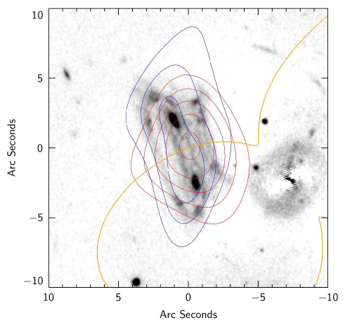
Figure 16: Velocity-integrated map of the CO(2–1) emission in A68-C0 overlaid on the HST image in band F110W. The extended blue contours are the contours integrated over the channels that define the blue-shifted component of the double-peaked CO emission line profile shown in Fig. 4 and the compact red contours are the contours integrated over the channels that define the red-shifted component of the CO profile. Contour levels start at $\pm 2\,\sigma$ and are in steps of $2\,\sigma$. The critical line (yellow line) is located right in the middle of the two multiple images easily identified by the two bright bulges resolved in the HST image.

A.2 A68-HLS115

The CO(2–1) line is also very well detected in A68-HLS115 as it can be seen in Figs. 3 and 4, with its intensity peaking at $14\,\sigma$. The CO(2–1) emission is nicely centred on the HST images to within $0.5^{\prime\prime}$. The HST images show that this $z_{\rm H\alpha}=1.5869$ galaxy has a very clumpy structure. The clumps are bright in the rest-frame UV, betraying intense star formation. Unfortunately they are unresolved in our CO observations, but would be of high interest for a deeper CO study at high spatial resolution.

The CO(2–1) spectrum reveals a strong emission line very well fitted by a single Gaussian function with a full width half maximum $\rm FWHM_{CO}=267\leavevmode\nobreak\ km\leavevmode\nobreak\ s^{-1}$ and an observed integrated flux $F_{\rm CO}=2.00\pm 0.30\leavevmode\nobreak\ \rm Jy\leavevmode\nobreak\ km\leavevmode\nobreak\ s^{-1}$. The measured CO redshift perfectly agrees with the H$\alpha$ redshift to within $\Delta z=(z_{\rm H\alpha}-z_{\rm CO})=0.001$. The derived lensing-corrected molecular gas fraction $f_{\rm gas}=0.75$ is very high; A68-HLS115 is among the gas-richer $z>1$ SFGs known (see Sect. 6). With a strong single-peaked CO emission line profile, we can hardly invoke evidence for rotation in this galaxy.

A.3 MACS0451-arc

The HST image reveals that this $z_{\rm H\alpha}=2.013$ galaxy is strongly stretched by gravitational lensing as testified by the striking, elongated arc extending over $20^{\prime\prime}$ and composed of multiple images of the source. We detect the CO(3-2) emission at $4-5\,\sigma$. It does not cover the entire arc, but is confined to the southern part of the arc (see Fig. 3). Such a confinement may either indicate that the lensing magnification is differential along the arc, and/or that the molecular gas is located in specific regions of the galaxy. The spatially resolved kinematics of this arc has been studied in detail with H$\alpha$ observations by Jones et al. (2010). This work allowed, in particular, to obtain a precise lens modelling and the reconstruction of the MACS0451-arc in the source plane. They show: (1) the southern part of the arc is the image of the whole source and it also corresponds to the image in which the central red region of the source, the region where most of the CO emission is likely to originate, is most strongly magnified; and (2) the northern part of the arc contains two images of the source very weakly magnified, in particular the central red region of the source is invisible in the HST images, the emission is dominated by one star-forming clump of the source close to the critical line which is popping up because of the increased magnification. Thus, the lack of CO detection in the northern part of the MACS0451-arc can be explained by the sensitivity limit of our PdBI data: if the total integrated CO flux of the southern part of the arc is detected at only $\rm S/N_{det}=4-5\,\sigma$, the northern part of the arc is expected to have an integrated CO flux below $2\,\sigma$ of the noise. We may conclude with confidence that the detected CO emission provides a good estimate of the total molecular gas content of this strongly-lensed galaxy. Finally, the small offset of $1^{\prime\prime}$ observed between the HST images and the CO emission, as well as the elongated shape of the CO emission which does not follow the exact orientation of the arc in HST images (see Fig. 3) are both most likely due to noise effects. Indeed, the low signal-to-noise ratio of the MACS0451-arc’s CO detection combined with the low spatial resolution of D-configuration data imply that only the detection itself is reliable, while any spatial information remains uncertain.

There is evidence that the MACS0451-arc contains an AGN component, as determined from the analysis of its IR SED. In particular, the southern part of the arc, which contains the most magnified image of the center of the source (as said above), shows a much hotter IR SED than the northern part of the arc. Indeed, while the SED of the northern part peaks at 250 $\mu$m, that of the southern part rises down to 100 $\mu$m (corresponding to a $\lambda_{\rm rest}<33$ $\mu$m). This excess of flux at short wavelengths indicates the presence of very hot dust, which cannot be reproduced by a stellar component only. By modelling the IR emission of the southern part, Zamojski et al. (in prep) find that roughly 55% of the IR-flux originates from an AGN, while the remaining 45% is coming from star formation. This is taken into account when estimating the total IR luminosity of the MAS0451-arc corrected from the AGN component (Table 1).

The CO(3–2) spectrum indicates the presence of a double-peaked emission line profile (see Fig. 4). The total full width half maximum is $\rm FWHM_{CO}=261\leavevmode\nobreak\ km\leavevmode\nobreak\ s^{-1}$ and the observed integrated flux $F_{\rm CO}=1.27\pm 0.32\leavevmode\nobreak\ \rm Jy\leavevmode\nobreak\ km\leavevmode\nobreak\ s^{-1}$. The measured CO redshift agrees very well with the H$\alpha$ redshift to within $\Delta z=(z_{\rm H\alpha}-z_{\rm CO})=0.0012$. The derived lensing-corrected molecular gas fraction $f_{\rm gas}=0.62$ is high, it is the higher among SFGs with CO measurements from the literature in the $\langle z_{2.2}\rangle=[2,2.5]$ interval (see Sect. 6.1).

The observed double-peaked CO emission line profile in the MACS0451-arc may appear as tentative because of the low $\rm S/N_{det}=4-5\,\sigma$, however the fit with two Gaussian functions is clearly favoured relative to the fit with a single Gaussian function. This prevents us from affirming conclusively whether the observed double-peaked CO emission line profile really originates from the presence of rotation (Daddi et al. 2010a), or is simply an artefact of a noisy line profile. Jones et al. (2010) showed that the kinematics of this galaxy as traced by the integrated H$\alpha$ emission line flux can be explained by rotation. Because, their data cover only part of the galaxy, either scenario, rotation versus merger, remains possible. The recent reconstructed morphology of the MACS0451-arc galaxy in the source plane found in Sklias et al. (2014) shows two tails, which can be most easily explained by a merger. Such a scenario would also naturally explain the presence of the AGN seen in the southern part of the arc.

A.4 A2218-Mult

This $z_{\rm H\beta}=3.104$ galaxy is the highest redshift galaxy from our sample of low-$L_{\rm IR}$ selected galaxies. HST images reveal two counterpart images (Richard et al. 2011). We searched for CO in the western counterpart image. Comparatively we achieved similarly deep PdBI observations with an rms of 0.77 mJy for this object, but the CO(3–2) emission remains undetected despite a high magnification factor $\mu=14$. We provide $4\,\sigma$ upper limits on the CO(3–2) integrated line flux and its respective derivatives CO(1–0) luminosity and molecular gas mass in Table 3. This object was not included in the study of Sklias et al. (2014), but we used the same tools and methods to derive its IR luminosity.

A.5 A68-h7

This $z_{\rm CO}=2.1529$ galaxy is less magnified with $\mu=3$ and characterized by a higher intrinsic IR luminosity $L_{\rm IR}=18.3\times 10^{11}\leavevmode\nobreak\ \rm L_{\sun}$ in comparison to the other galaxies from our sample. It has thus been observed at the IRAM 30 m telescope. The CO(3–2) spectrum shows a broad line detected at $3-4\,\sigma$ and well fitted by a single Gaussian function (see Fig. 4). It has a full width half maximum $\rm FWHM_{CO}=282\leavevmode\nobreak\ km\leavevmode\nobreak\ s^{-1}$ and an observed integrated flux $F_{\rm CO}=1.12\pm 0.22\leavevmode\nobreak\ \rm Jy\leavevmode\nobreak\ km\leavevmode\nobreak\ s^{-1}$. A redshift offset is observed in A68-h7 between the CO redshift and the redshift determined in this case from weak absorption lines in the rest-frame UV, $\Delta z=(z_{\rm rest-UV}-z_{\rm CO})=-0.0029$. This offset is not surprising, because interstellar medium lines are expected to be blueshifted with respect to the systemic redshift of the galaxy as set here by the CO(3–2) line in presence of outflows (Quider et al. 2009; Dessauges-Zavadsky et al. 2010). The derived lensing-corrected molecular gas fraction $f_{\rm gas}=0.33$ is comparable to the $f_{\rm gas}$ distribution of SFGs with CO measurements from the literature in the $\langle z_{2.2}\rangle=[2,2.5]$ interval which has a mean $\langle f_{\rm gas}^{\langle z_{2.2}\rangle}\rangle=0.45\pm 0.22$ (see Sect. 6.1).

The observed double-peaked CO emission line profile, which would require higher signal-to-noise ratio data to be confirmed (in particular for the second component sampled by two channels only given its small full width half maximum $\rm FWHM_{CO}=90\leavevmode\nobreak\ km\leavevmode\nobreak\ s^{-1}$; see Fig. 4), sustains evidence for rotation in A68-h7 (Daddi et al. 2010a). Its morphology in the HST images reveals several components, which probably all contribute to the CO emission signal and may be the analogues of giant star-forming clumps seen in disk-like simulated systems (Agertz et al. 2009; Genel et al. 2010; Bournaud et al. 2011).

A.6 cB58 and Eye

We adopt for these two strongly-lensed galaxies at $z_{\rm H\alpha}=2.729$ and 3.0733, respectively, the CO(1–0) integrated fluxes obtained with the Expanded Very Large Array (EVLA) by Riechers et al. (2010). The Eye is one of the rare $z>3$ star-forming galaxies with a CO detection. Detections of the CO(3–2) line with the PdBI and measurements of their respective integrated fluxes were also reported by Baker et al. (2004) in cB58 and Coppin et al. (2007) in the Eye. Those are used in Sect. 4 to study the CO luminosity correction factors of star-forming galaxies at $z>1$. Combined with our updated stellar masses from Sklias et al. (2014), we infer lensing-corrected molecular gas fractions $f_{\rm gas}=0.41$ in cB58 and $f_{\rm gas}=0.18$ in the Eye. Although they are very similar to the molecular gas fractions reported by Riechers et al. (2010), $f_{\rm gas}=0.32$ in cB58 and $f_{\rm gas}=0.13$ in the Eye, if we consider the stellar masses assumed by Riechers et al. and our prescriptions for the CO luminosity correction factor and the CO–H₂ conversion factor, the corresponding molecular gas fractions get significantly higher by a factor of 2 and 2.5, respectively, compared to ours. The revised molecular gas fraction of the Eye is particularly low, it is the lowest among $z>1$ SFGs with CO measurements from the literature (see Sect. 6). This may partly be attributed to the “post-starburst” nature of the Eye as inferred by Sklias et al. (2014) from a detailed SED analysis.