Polynomial size linear programs for problems in P

Abstract

A perfect matching in an undirected graph $G=(V,E)$ is a set of vertex disjoint edges from $E$ that include all vertices in $V$. The perfect matching problem is to decide if $G$ has such a matching. Recently Rothvoß proved the striking result that the Edmonds’ matching polytope has exponential extension complexity. In this paper for each $n=|V|$ we describe a polytope for the perfect matching problem that is different from Edmonds’ polytope and define a weaker notion of extended formulation. We show that the new polytope has a weak extended formulation (WEF) $Q$ of polynomial size. For each graph $G$ with $n$ vertices we can readily construct an objective function so that solving the resulting linear program over $Q$ decides whether or not $G$ has a perfect matching. With this construction, a straightforward $O(n^{4})$ implementation of Edmonds’ matching algorithm using $O(n^{2})$ bits of space would yield a WEF $Q$ with $O(n^{6}\log n)$ inequalities and variables. The construction is uniform in the sense that, for each $n$, a single polytope is defined for the class of all graphs with $n$ nodes. The method extends to solve polynomial time optimization problems, such as the weighted matching problem. In this case a logarithmic (in the weight of the optimum solution) number of optimizations are made over the constructed WEF.

The method described in the paper involves the construction of a compiler that converts an algorithm given in a prescribed pseudocode into a polytope. It can therefore be used to construct a polytope for any decision problem in P which can be solved by a well defined algorithm. Compared with earlier results of Dobkin-Lipton-Reiss and Valiant our method allows the construction of explicit linear programs directly from algorithms written for a standard register model, without intermediate transformations. We apply our results to obtain polynomial upper bounds on the non-negative rank of certain slack matrices related to membership testing of languages in P/poly.

s¿c

1 Introduction

A perfect matching in an undirected graph $G=(V,E)$ is a set of vertex disjoint edges from $E$ that include all vertices in $V$. We let $n$ denote the number of vertices and assume $n$ is even throughout the paper. The perfect matching problem is to determine if $G$ contains a perfect matching and this can be decided in polynomial time by running Edmonds’ algorithm [9]. As well as this combinatorial algorithm, Edmonds also introduced a related polytope [10] which we will call the Edmonds’ polytope $\mathrm{EP}_{n}$:

$$\mathrm{EP}_{n}=\operatorname{CH}\{x\in\{0,1\}^{\binom{n}{2}}:x~{}\text{is the edge-vector of a perfect matching in }K_{n}\}$$ (1)

where $\operatorname{CH}$ is the convex hull operator.

For any $S\subseteq V$ and edge $ij\in E$, we write that $ij\in\delta(S)$ whenever exactly one of the vertices $i$ and $j$ is in $S$. Edmonds [10] proved that $\mathrm{EP}_{n}$ has the following halfspace representation:

$$\sum_{ij\in\delta(S)}x_{ij} \geqslant 1,~{}~{}~{}~{}~{}~{}~{}~{}~{}~{}~{}~{}~{}S\subseteq V,~{}|S|\geqslant 3,~{}|S|~{}is~{}odd$$

$$\sum_{ij\in\delta(i)}x_{ij} = 1~{}~{}~{}~{}~{}~{}~{}~{}~{}~{}~{}~{}~{}i=1,2,...,n$$

$$0\leqslant x_{ij} \leqslant~{}1,~{}~{}~{}~{}~{}~{}1\leqslant i<j\leqslant n$$

This description is exponential in size. Nevertheless, the perfect matching problem can be solved in polynomial time by solving a linear program (LP) over this polytope. Indeed, define an objective function $c^{T}x=\sum_{1\leqslant i<j\leqslant n}c_{ij}x_{ij}$, where $c_{ij}=1$ if $ij\in E$ and $c_{ij}=0$ otherwise. The LP is:

$$z^{*}= \max ~{}c^{T}x$$

$$s.t. x\in\mathrm{EP}_{n}$$

It is easy to verify that if $G$ has a perfect matching then $z^{*}=n/2$ otherwise $z^{*}<n/2$. Since the inequalities defining $\mathrm{EP}_{n}$ can be separated in polynomial time, the LP can be solved in polynomial time [14].

Since the perfect matching problem is in P, it seemed possible that $\mathrm{EP}_{n}$ could be written as the projection of a polytope with a polynomial size description. This is the topic of extension complexity (see, e.g., Fiorini et al. [12]). We recall the basic definitions here, referring the reader to [12] for further details.

An extended formulation (EF) of a polytope $Q\subseteq{\mathbb{R}}^{q}$ is a linear system

$$Ex+Fy=g,\ y\geqslant\mathbf{0}$$ (3)

in variables $(x,y)\in{\mathbb{R}}^{q+r},$ where $E,F$ are real matrices with $q,r$ columns respectively, and $g$ is a column vector, such that $x\in Q$ if and only if there exists $y$ such that (3) holds. The size of an EF is defined as the number of inequalities in the system.

An extension of the polytope $Q$ is another polytope $Q^{\prime}\subseteq\mathbb{R}^{e}$ such that $Q$ is the image of $Q^{\prime}$ under a linear map. We define the size of an extension $Q^{\prime}$ as the number of facets of $Q^{\prime}$. Furthermore, we define the extension complexity of $Q$, denoted by $\mathop{\mathrm{xc}}{(Q)},$ as the minimum size of any extension of $Q.$

Rothvoß [18] recently proved the surprising result that $\mathop{\mathrm{xc}}{(\mathrm{EP}_{n})}$ is exponential. Since extension complexity seemed a promising candidate to obtain computational models that separate problems in P from those that are NP-hard, this was a setback. A way of strengthening extension complexity to handle this problem was recently proposed by Avis and Tiwary [3].

Dobkin et al. [8] and Valiant [19] showed that linear programming is P-complete from which it follows that every problem in P has an LP-formulation of polynomial size. We will review this result in Section 3 giving Valiant’s construction. This construction applies to P/poly, which is the class of all decision problems $L$ solvable by a family $C_{n},n\geq 1$ of polynomial size Boolean circuits such that $C_{n}$ solves the restriction of $L$ to inputs of length $n$. From these circuits it is straightforward to construct a family of LPs.

The main contribution of this paper is to give a direct method to produce polynomial size LPs from polynomial time algorithms, not circuits. Specifically we will construct LPs directly from a polynomial time algorithm expressed in pseudocode that solves a decision problem. Of course a trivial LP formulation can be obtained by first solving the decision problem for a given input and setting $c=1$ if the answer is yes and $c=0$ otherwise. Then solving the one dimensional LP: $\max~{}cx,0\leqslant x\leqslant 1$ solves the original problem. To avoid such trivial LPs we limit how much work can be done in constructing the objective function. One such limitation might be, for example, to insist that the objective function can be computed in linear time in terms of the input size. The objective functions we consider in this paper satisfy this condition.

For concreteness, we focus on an explicit construction of a polynomial size LP that can be used to solve the perfect matching problem. Firstly we describe another ‘natural’ polytope, $\mathrm{PM}_{n}$, for the perfect matching problem. Then we will introduce the notion of a weak extended formulation (WEF). Instead of requiring projection onto $\mathrm{PM}_{n}$ we will simply require that LPs solved over the WEF solve the original problem. The objective function used is basically just a $\pm 1$ encoding of the input graph. The approach used is quite general and can be applied to any problem in $P$ for which an explicit algorithm is known. It extends to polynomial time solvable optimization problems also. However in this case a logarithmic (in the weight of the optimum solution) number of optimizations are made over the constructed WEF. Note that when an EF exists both the optimization and decision problems can be solved in a single LP optimization. Hence a WEF is weaker since a single LP solves only the decision problem. We discuss this further in Section 6.

The paper is organized as follows. In the next section we introduce a new polytope for the perfect matching problem and give some basic results about its facet structure. We define the notion of weak extended formulation and state the main theorem. In Section 3 we first give a simple example to illustrate the technique we use to build extended formulations from boolean circuits. Then we prove the main theorem of the paper. In Section 4 we generalize our method to algorithms given in pseudocode rather than as a circuit. We show how programs written in a simple pseudocode can be converted to WEFs. Our method is modeled on Sahni’s proof of Cook’s theorem given in [15]. Since our pseudocode is clearly strong enough to implement Edmonds’ algorithm in polynomial time, our method gives a polynomial size WEF for the perfect matching problem. In Section 5 we use our main theorem to show that the non-negative rank of certain matrices is polynomially bounded above. Finally in Section 6 we give some concluding remarks including a discussion of applying this technique to polynomial time optimization problems such as the maximum weighted matching problem.

2 Polytopes for decision problems

2.1 Another perfect matching polytope

We use the notation $\mathds{1}_{t}$ to denote the $t$-dimensional vector of all ones, dropping the subscript when it is clear from the context. Let $n$ be an even integer and let $x$ be a binary vector of length $\binom{n}{2}$. We let $G(x)=(V,E)$ denote the graph with edge incidence vector given by $x$, let $n$ be the number of its vertices and $m=\mathds{1}^{T}x$ the number of its edges. Furthermore, let $w_{x}=1$ if $G(x)$ has a perfect matching and zero otherwise. We define the polytope $\mathrm{PM}_{n}$ as:

$$\mathrm{PM}_{n}=\operatorname{CH}\{(x,w_{x}):x\in\{0,1\}^{\binom{n}{2}}\}.$$ (4)

$\mathrm{PM}_{n}$ may be visualized by starting with a hypercube in dimension $\binom{n}{2}$ and embedding it in one higher dimension with extra coordinate $w$. For vertices of the cube corresponding to graphs with perfect matchings $w=1$ else $w=0$. It is easy to see that $\mathrm{PM}_{n}$ has precisely $2^{\binom{n}{2}}$ vertices. Edmonds’ polytope $\mathrm{EP}_{n}$ is closely related to $\mathrm{PM}_{n}$, in fact it defines one of its faces. Let

$$F_{n}=\mathrm{PM}_{n}\cap\{(x,w):\mathds{1}^{T}x+(1-w)n^{2}=\frac{n}{2}~{}\}$$ (5)

Proposition 1.

$F_{n}$ defines a face of $\mathrm{PM}_{n}$ and in fact

$$F_{n}=\{(x,1):x\in\mathrm{EP}_{n}\}.$$ (6)

Proof.

To show that $F_{n}$ is a face we show that the inequality

$$\mathds{1}^{T}x+(1-w)n^{2}\geqslant\frac{n}{2}$$ (7)

is valid for $\mathrm{PM}_{n}$. It suffices to verify it for the extreme points $(x,w_{x})$ given in (4). If $w_{x}=0$, (7) holds since $\mathds{1}^{T}x+n^{2}>\frac{n}{2}$. Since the inequality is strict, none of these extreme points lie on $F_{n}$. Otherwise $w_{x}=1$, $x$ is the incidence vector of graph containing a perfect matching, so $\mathds{1}^{T}x\geqslant n/2$. This shows that $F_{n}$ defines a face of $\mathrm{PM}_{n}$.

The vectors $x$ with $w_{x}=1$ and $\mathds{1}^{T}x=n/2$ are the incidence vectors of perfect matchings of $K_{n}$ and are precisely those used to define $\mathrm{EP}_{n}$ in (1). Hence $\mathrm{EP}_{n}$ lifted by adding the coordinate $w=1$ is precisely $F_{n}$. ∎

For a given input graph $G(\bar{x})=(V,E)$ we define the vector $c=(c_{ij})$ as follows:

$$c_{ij}=\begin{cases}~{}~{}1&\text{if $ij\in E$}\\ -1&\text{otherwise}\end{cases}~{}~{}~{}~{}~{}~{}~{}~{}~{}~{}1\leq i<j\leq n$$ (8)

and let $d$ be a constant such that $0<d\leqslant 1/2$. We construct the LP:

$$z^{*}= \max ~{}c^{T}x+dw$$

$$s.t. (x,w)\in\mathrm{PM}_{n}$$

For any positive integer $n$, by an $n$-cube we mean the $n$-dimensional hypercube whose vertices are the $2^{n}$ binary vectors of length $n$.

Proposition 2.

For any edge incidence vector $\bar{x}\in\{0,1\}^{\binom{n}{2}}$ let $m=\mathds{1}^{T}\bar{x}$. The optimum solution to (2.1) is unique, $z^{*}=m+d$ if $G(\bar{x})$ has a perfect matching, and $z^{*}=m$ otherwise.

Proof.

Let $c$ be the vector defined by (8) and set $m=\mathds{1}^{T}\bar{x}$. Note that $c^{T}\bar{x}=m$ and that $c^{T}x\leqslant m-1$ for any other vertex $x$ of the $\binom{n}{2}$-cube. If $G(\bar{x})$ has a perfect matching then $(x,w)=(\bar{x},1)$ is a feasible solution to (2.1) with $z=m+d$. Since $x\neq\bar{x}$, $c^{T}x+dw\leqslant m-1+d$ and so $(\bar{x},1)$ is the unique optimum solution.

If $G(\bar{x})$ does not have a perfect matching then $(x,w)=(\bar{x},0)$ is a feasible solution to (2.1) with $z=m$. Consider any other vertex $x$ of the $\binom{n}{2}$-cube. Then $z=c^{T}x+dw\leqslant m-1+1/2=m-1/2$. It follows that $z^{*}=m$ and is obtained by the unique solution $(\bar{x},0)$. ∎

2.2 Polytopes for decision problems and weak extended formulations

The basic ideas above can be extended to arbitrary polynomial time decision problems. Let $X$ denote a polynomial time decision problem defined on binary input vectors $x=(x_{1},...,x_{q})$, and an additional bit $w_{x}$, where $w_{x}=1$ if $x$ results in a “yes” answer and $w_{x}=0$ if $x$ results in a “no” answer. We define the polytope $P$ as:

$$P=\operatorname{CH}\{(x,w_{x}):x\in\{0,1\}^{q}\}$$ (10)

For a given binary input vector $\bar{x}$ we define the vector $c=(c_{j})$ by:

$$c_{j}=\begin{cases}~{}~{}1&\text{if}~{}\bar{x}_{j}=1\\ -1&\text{if}~{}\bar{x}_{j}=0\end{cases}~{}~{}~{}~{}~{}~{}~{}~{}~{}~{}1\leq i<j\leq n$$ (11)

and let $d$ be a constant such that $0<d\leqslant 1/2$. As before we construct an LP:

$$z^{*}= \max ~{}c^{T}x+dw$$

$$s.t. ~{}(x,w)\in P$$

The following proposition can be proved in an identical way to Proposition 2.

Proposition 3.

For any $\bar{x}\in\{0,1\}^{q}$ let $m=\mathds{1}^{T}\bar{x}$. The optimum solution to (2.2) is unique, $z^{*}=m+d$ if $\bar{x}$ has a “yes” answer and $z^{*}=m$ otherwise.

Definition 1.

Let $Q$ be a polytope which is a subset of the $(q+t)$-cube with variables labeled $x_{1},...,x_{q},y_{1},...,y_{t}$. We say that $Q$ has the x-0/1 property if each of the $2^{q}$ ways of assigning 0/1 to the variables $x_{1},...,x_{q}$ uniquely extends to a vertex $(x,y)$ of $Q$ and, furthermore, $y$ is 0/1 valued. $Q$ may have additional fractional vertices.

In polyhedral terms, for every binary vector $b\in{\mathbb{R}}^{q}$, the intersection of $Q$ with the hyperplanes $x_{j}=b_{j}$ is a 0/1 vertex. We will show that we can solve a polynomial time decision problem $X$ by replacing $P$ in (2.1) by a polytope $Q$ of polynomial size, while maintaining the same objective functions. We call $Q$ a weak extended formulation as it does not necessarily project onto $P$.

Definition 2.

A polytope

$$Q=\{(x,w,s):x\in[0,1]^{q},w\in[0,1],s\in[0,1]^{r},Ax+bw+Cs\leqslant h\}$$

is a weak extended formulation (WEF) of $P$ if the following hold:

• $Q$ has the $x$-0/1 property.

• For any vector $\bar{x}\in\{0,1\}^{q}$ let $m=\mathds{1}^{T}\bar{x}$, let $c$ be defined by (11) and let $0<d\leqslant 1/2$. If $\bar{x}$ has a “yes” answer the optimum solution of the LP

  $$z^{*}=\max~{}\{c^{T}x+dw:(x,w,s)\in Q\}$$ (13)

  is unique and takes the value $z^{*}=m+d$. Otherwise $z^{*}<m+d$.

The first condition states that any vertex of $Q$ that has 0/1 values for the $x$ variables has 0/1 values for the other variables as well. The second condition connects $Q$ to $P$. For a 0/1 valued vertex $(x,w,s)$ of $Q$ we have $w=1$ if $x$ encodes a “yes” answer since $z^{*}=m+d$. If $x$ encodes a “no” answer then $z^{*}<m+d$ and we must have $w=0$. The purpose of the coefficient $d$ is so that we can distinguish the two answers by simply observing the value of $z^{*}$.

In the sequel we will be concerned with small positive constants which we will assume are rational and in reduced form $d=p/q$, for positive integers $p$ and $q$. The size of $d$ is $\lceil\log_{2}p\rceil+\lceil\log_{2}q\rceil$.

In general $Q$ will have fractional vertices and that is why the condition for “no” answers differs from that given in Proposition 3 (an example is given below). However, for small enough $d$ we can ensure that the LP optimum solution is unique in both cases and corresponds to that given in Proposition 3.

Proposition 4.

Let $Q$ be a WEF of $P$. There is a positive constant $d_{0}$, whose size is polynomial in the size of $Q$, such that for all $d$, $0<d<d_{0}$, the optimal solution of the LP defined in (13) is unique, $z^{*}=m+d$ if $\bar{x}$ has a “yes” answer and $z^{*}=m$ if $\bar{x}$ has a “no” answer.

Proof.

The part of the proposition relating to the “yes” answers is already covered by Definition 2. So consider any $\bar{x}$ corresponding to a “no” answer and its associated vector $c$ given by (11). Since $Q$ has the 0/1 property $\bar{x}$ uniquely extends to a 0/1 valued vertex $(\bar{x},\bar{w},\bar{s})$ of $Q$ with $\bar{w}=0$ as we saw above. So for any $d$, $0<d\leq 1/2$, we have $c^{T}\bar{x}+d\bar{w}=c^{T}\bar{x}=m$. Consider any other vertex $(x,w,s)$ of $Q$. Since $x\neq\bar{x}$, we have $c^{T}x<m$. Let $d({\bar{x}})=\min\{m-c^{T}x\}$ taken over all vertices $(x,w,s)$ with $x\neq\bar{x}$. This minimum exists, since the number of vertices of $Q$ is finite, and is positive. Furthermore, $c^{T}x+d({\bar{x}})w\leq c^{T}x+d({\bar{x}})\leq m$. We define

$$d_{0}=\min\{d(y)~{}:~{}y\in\{0,1\}^{q}~{}\text{has a ``no'' answer}\}.$$

Now choose any $d$, $0<d<d_{0}$, and any vertex $(x,w,s)$ of $Q$ with $x\neq\bar{x}$. If $w>0$ then $c^{T}x+dw<c^{T}x+d_{0}w\leq c^{T}x+d_{0}\leq m$. Otherwise $w=0$ and we have $c^{T}x+dw=c^{T}x<m$ as noted above. Since the optimal solution for any LP can always be obtained at a vertex, it follows that the LP defined in (13) has a unique optimum solution $z^{*}=m$ whenever $\bar{x}$ corresponds to a “no” answer.

If follows from standard linear programming theory that each vertex $(x,w,s)\in Q$ can be represented by a number of bits polynomial in the size of $Q$. Since $c$ is a $\pm 1$ vector and $m\leq n$ it follows that $m-c^{T}x$ can also be so represented. Now $d_{0}$ is the minimum of a finite number of such quantities so has size polynomial in the size of $Q$. The proposition follows. ∎

This proof gives, at least in principle, a method of computing the constant $d_{0}$ from a list of the vertices of $Q$. An easier to compute bound can be obtained from the analysis of Khachian’s ellipsoid method, see, for example, the text [14]. Following this text, let $\langle{}Q\rangle{}$ be the number of bits required to represent $Q$. Then the proof of their Lemma 3.1.33 implies that the differences $m-c^{T}x$ in the above proof are all at least $2^{-\langle{}Q\rangle{}}$ and so we could choose this value for $d$. This value will generally be much too small to be of practical use. However, if we are able to observe the value of $w$ in the optimum solution of (13) then we may in fact set $d=0$. In this case $z^{*}=m$ for both answers and it follows from the 0/1 property that the optimum solution is unique and 0/1 valued. Since $Q$ is a WEF of $P$ the value of $w$ in the optimum solution gives the correct answer. This is the preferred method in practice as it reduces the problem of floating point round off errors which may be caused by small values of $d$.

We saw in the proof of Proposition 4, the reason that $d$ has to be small is to ensure that fractional vertices of $Q$ do not lead to optimum solutions for $\pm 1$ valued object vectors $c$. As an example, consider the perfect matching problem and the polytope $\mathrm{PM}_{n}$ defined earlier. Suppose $Q_{n}$ is a WEF for $\mathrm{PM}_{n}$. It follows from Propositions 2 and 4 that we can determine whether an input graph $G$ has a perfect matching by solving an LP over either $\mathrm{PM}_{n}$ or $Q_{n}$ using the same objective function which is derived directly from the edge adjacency vector of $G$. As a very simple case, consider $n=2$ giving $\mathrm{PM}_{2}=\operatorname{CH}\{(0,0),(1,1)\}$. A possible WEF with $r=0$ is given by:

$$Q_{2}=\operatorname{CH}\{(0,0,0),(1,1,1),(1/4,1,1/2)\}$$

Initially let $d=1/2$. When $G(\bar{x})$ is an edge, $m=1$, $c_{12}=1$ and $z=c^{T}x+dw$ obtains the same optimum solution of $z^{*}=3/2=m+d$ over both $\mathrm{PM}_{2}$ and $Q_{2}$. When $G(\bar{x})$ is a non-edge, $m=0$, $c_{12}=-1$ and $z=c^{T}x+dw$ obtains the optimum solution of $z^{*}=0=m$ over $\mathrm{PM}_{2}$ and $z^{*}=1/4<1/2=m+d$ over $Q_{2}$, at the fractional vertex (1/4,1,1/2). However, if $0<d<1/4$ then $z=c^{T}x+dw$ is negative for the fractional vertex and obtains the unique optimum solution of $z^{*}=0=m$ over $Q_{2}$ and also, of course, over $\mathrm{PM}_{2}$. We see that $Q_{2}$ projects onto a triangle in the $(x,w)$-space, whereas $\mathrm{PM}_{2}$ is a line segment.

In the next section we prove the following result:

Theorem 1.

Every decision problem $X$ in P/poly admits a weak extended formulation $Q$ of polynomial size.

3 From Circuits to Polytopes

In order to show that Linear Programming is P-complete, Valiant [19] gave a construction to transform boolean circuits into a linear sized set of linear inequalities with the $x$-0/1 property (where $x_{i}$ are the variables corresponding to the inputs of the circuit); a similar construction was used by Yannakakis [20] in the context of the Hamiltonian Circuit problem. In this section we show that Valiant’s construction implies Theorem 1. Valiant’s point of view is slightly different from ours in that he explicitly fixes the values of the input variables before solving an LP-feasibility problem (as opposed to using different objective functions with a fixed set of inequalities). Showing that the result of this fixing is a $0/1$-vertex is precisely our $x$-0/1 property.

We begin with a standard definition, see for example the text by Arora and Barak [1]:

Definition 3.

A (boolean) circuit with $q$ input bits $x=(x_{1},x_{2},...,x_{q})$ is a directed acyclic graph in which each of its $t$ nodes, called gates, is either an AND ($\wedge$) gate, an OR ($\vee$) or a NOT ($\neg$) gate. We label each gate by its output bit. One of these gates is designated as the output gate and gives output bit $w$. The size of a circuit is the number of gates it contains and its depth is the maximal length of a path from an input gate to the output gate.

For example, the circuit shown in Figure 1 can be used to compute whether or not a graph on 4 nodes has a perfect matching. The input is the binary edge-vector of the graph and the output is $w=1$ if the graph has a matching (e.g. $G_{1}$) or $w=0$ if it does not (e.g. $G_{2}$). If the graph has a perfect matching, exactly one of $y_{12},y_{13}$ or $y_{14}$ is one, defining the matching. For each gate we have labeled the output bit by a new variable. We will construct a polytope from the circuit by constructing a system of inequalities on the same variables.

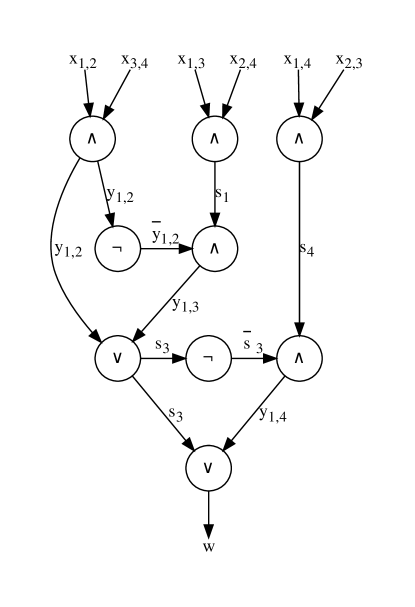
Figure 1: A circuit to compute whether a 4 node graph has a perfect matching

From an AND gate, say $y_{12}=x_{12}\wedge x_{34}$, we generate the inequalities:

$$x_{12}+x_{34}-y_{12} \leqslant 1$$

$$-x_{12}~{}~{}~{}~{}~{}~{}~{}~{}+y_{12} \leqslant 0$$ (14)

$$~{}~{}~{}~{}~{}~{}~{}-x_{34}+y_{12} \leqslant 0$$

$$y_{12} \geqslant 0$$

The system (14) defines a polytope in three variables whose 4 vertices represent the truth table for the AND gate:

$$x_{12} ~{}~{}x_{34}~{}~{}~{}~{}y_{12}$$

$$0 ~{}~{}~{}0~{}~{}~{}~{}~{}~{}0$$

$$0 ~{}~{}~{}1~{}~{}~{}~{}~{}~{}0$$

$$1 ~{}~{}~{}0~{}~{}~{}~{}~{}~{}0$$

$$1 ~{}~{}~{}1~{}~{}~{}~{}~{}~{}1$$

Note that the variables $x_{12},x_{34}$ define a 2-cube and so the polytope is an extension of the 2-cube. In the terminology of the last section, it has the $\{x_{12},x_{34}\}$-0/1 property.

From an OR gate, say $s_{3}=y_{12}\vee y_{13}$, we generate the inequalities:

$$-y_{12}-y_{13}+s_{3} \leqslant 0$$

$$y_{12}~{}~{}~{}~{}~{}~{}~{}-s_{3} \leqslant 0$$ (15)

$$~{}~{}~{}~{}~{}~{}y_{13}-s_{3} \leqslant 0$$

$$s_{3} \leqslant 1$$

The system (15) defines a polytope in three variables whose 4 vertices represent the truth table for the OR gate, as can easily be checked. Indeed, this polytope has the $\{y_{12},y_{13}\}$-0/1 property.

From a NOT gate, say $\bar{y}_{12}=\neg y_{12}$, we could generate the equation

$$\bar{y}_{12}=1-y_{12}$$ (16)

However it is equivalent to just replace all instances of $\bar{y}_{12}$ by $1-y_{12}$ in the inequality system, and this is what we will do in the sequel.

The circuit in Figure 1 contains 5 AND gates and 2 OR gates. By suitably replacing variables in (14) and (15) we obtain a system of 28 inequalities in 13 variables. As just mentioned, the NOT gates are handled by variable substitution rather than explicit equations. Let $Q_{4}$ denote the corresponding polytope. It will follow by the general argument below that $Q_{4}$ is a weak extended formulation (WEF) of $\mathrm{PM}_{4}$.

We now show that the above construction can be applied to any boolean circuit $C$ to obtain a polytope $Q$ which has the 0/1 property with respect to the inputs of $C$.

Lemma 1 ([19]).

Let $C$ be a boolean circuit with $q$ input bits $x=(x_{1},x_{2},...,x_{q})$, $t$ gates labeled by their output bits $y=(y_{1},y_{2},...,y_{t})$ and with circuit output bit $w=y_{t}$. Construct the polytope $Q$ with $4t$ inequalities and $q+t$ variables using the systems (14) and (15) respectively. $Q$ has the the $x$-0/1 property and for every input $x$ the value of $w$ computed by $C$ corresponds to the value of $y_{t}$ in the unique extension $(x,y)\in Q$ of $x$.

Proof.

Since $C$ is an acyclic directed graph it contains a topological ordering of its nodes (gates) and we can assume that the labeling $y_{1},y_{2},...,y_{t}$ is such an ordering. Note we can assume $w=y_{t}$ comes last since it cannot be an input to any other gate. For any given input $x$ the output of the circuit can be obtained by evaluating each gate in the order $y_{1},...,y_{t}$. Since it is a topological ordering, each input for a gate has been determined before the gate is evaluated.

We proceed by induction. Let $Q_{k}$ be the polytope defined by the $4k$ inequalities corresponding to gates $y_{1},...,y_{k}$. The inductive hypothesis is that for $k=1,2,...,t$

• $Q_{k}$ has the $x$-0/1 property, and

• for each $x$ the value of $y_{k}$ calculated by $C$ corresponds to the value of $y_{k}$ in the unique extension of $x$ in $Q_{k}$.

This is clearly true for $k=1$ as the analysis following (14) and (15) shows. We assume the hypothesis is true for $k=1,2,...,j$, where $1\leqslant j<t$, and prove it for $j+1$. Indeed, since $Q_{j}$ has the $x$-0/1 property for each $x$ the values of $y_{1},...,y_{j}$ are uniquely defined and have 0/1 values. By induction they correspond to the values computed by $C$. Therefore the analysis following (14) and (15) shows that $y_{j+1}$ will also be uniquely defined, 0/1 valued, and will correspond to the value computed by $C$. This verifies the inductive hypothesis for $j+1$ and since $Q=Q_{t}$ the proof is complete. ∎

Lemma 2.

Let $C$ be a circuit that solves a decision problem $X$ with $q$ input bits $x=(x_{1},x_{2},...,x_{q})$ and has associated polytope $P$ as defined in (10). The polytope $Q$ constructed in Lemma 1 is a WEF for $P$.

Proof.

In order to make the correspondence with Definition 2 we relabel the variables in $Q$, constructed in Lemma 1, so that $s=(y_{1},y_{2},...,y_{t-1})$ and $w=y_{t}$. By Lemma 1 we know $Q$ has the $x$-0/1 property so it remains to prove the second condition in Definition 2.

Let $\bar{x}$ be any vector in $\{0,1\}^{q}$ and set $m=\mathds{1}^{T}\bar{x}$. Since $Q$ has the $x$-0/1 property $\bar{x}$ extends to a unique binary vertex $(\bar{x},\bar{w},\bar{s})$ of $Q$. Define $c$ as in (11). Fix some $d$, $0<d\leqslant 1/2$ and consider the optimum solution

$$z^{*}=\max~{}\{c^{T}x+dw:(x,w,s)\in Q\}.$$

Since $Q$ has the $x$-0/1 property the maximum of $c^{T}x$ over $Q$ is obtained at $c^{T}\bar{x}=m$ at the unique vertex $(\bar{x},\bar{w},\bar{s})$ of $Q$. For any other $(x,w,s)\in Q$, since $x$ is in the $q$-cube and not equal to $\bar{x}$, we have $c^{T}x<m$ and, since $w\leqslant 1$, $z=c^{T}x+dw<m+d$. Therefore, if $\bar{x}$ has a “yes” answer then $w=1$, $z^{*}=m+d$ and $(\bar{x},\bar{w},\bar{s})$ is the unique optimum solution. Otherwise $z^{*}<m+d$. The lemma follows. ∎

Theorem 1 follows from Lemmas 1 and 2. Since there is no limitation of uniformity on the circuits used, the theorem holds for all decision problems in P/poly. Since each gate in the circuit gives rise to 4 inequalities and one new variable, we have the following corollary.

Corollary 1.

Let $X$ be a decision problem with corresponding polytope $P$ defined by (10). A set of circuits for $X$ with size $p(n)$ generates a WEF $Q$ for $P$ with at most $4p(n)$ inequalities and variables.

In this section we showed how to construct a polynomial size LP from a polynomial size circuit so that the optimum solution of the LP gives the output of the circuit. However it is not immediately clear how to use this to obtain a polytope for the perfect matching problem. It would be required to convert Edmonds’ algorithm to a family of circuits. In the next section we bypass this step by showing how to convert a simple pseudocode directly into a polytope without first computing a circuit (See Theorem 2). This can be used to convert polynomial time algorithms into polynomial size LPs directly.

We would like to remark that our construction in Theorem 2 of a WEF from a pseudocode may not be optimal. For example, it would be possible to get roughly $O(T(n)\log T(n))$- size circuits simulating a given $T(n)$-time bounded Turing machine (see, e.g., Chapter 1 of [1]) from which we can construct a WEF with $O(T(n)\log T(n))$ inequalities. But since Turing Machines are not commonly used for designing algorithms, we leave the interested reader to check whether a similar idea can be used to define a WEF with smaller size.

4 Constructing an LP from pseudocode

In this section we introduce a rudimentary pseudocode that can be used for decision problems. This pseudocode follows the usual practices of specifying algorithms and the tradition of so-called register machines (see e.g. [7]). We show how the code can be translated into a linear program, in a way similar to that shown for circuits in the previous section. This translation works for any pseudocode, but since the focus of this paper is on the class P, we will assume there is a polynomial function $p(n)$ so that the the code terminates within $p(n)$ steps for any input of size $n$. In this case we will show that the corresponding LP will also have polynomial size in $n$.

The pseudocode we use and its translation into an LP is adapted from a proof of Cook’s theorem given in [15] which is attributed to Sartaj Sahni. In Sahni’s construction the underlying algorithm may be non-deterministic, but we will consider only deterministic algorithms. Furthermore, Sahni describes how to convert his pseudocode into a satisfiability expression. Although it would be possible to convert this expression into an LP, considerable simplifications are obtained by doing a direct conversion from pseudocode to an LP. In this section, for simplicity, we describe only those features of the pseudocode that are necessary for implementing Edmonds’ algorithm for the perfect matching problem. Additional features would be needed to handle more sophisticated problems, such as the weighted matching problem. For full details, the reader is referred to Section 11.2 of [15].

Our pseudocode ${\mathtt{A}}$ has the following form. We assume $W$ is a fixed integer which will represent the word size for integer variables.

• Variables are binary valued except for indices, which are $W$-bit integers. Arrays of binary values are allowed and may be one or two dimensional. Dimension information is specified at the beginning of ${\mathtt{A}}$. We let $q(n)$ denote the maximum number of bits required to represent all variables for an input size of $n$. Sahni argues that $q(n)=O(p(n))$ however in our case $q(n)$ is significantly smaller. Statements in ${\mathtt{A}}$ are numbered sequentially from $1$ to $l$.

• An expression contains at most one boolean operator or is the incrementation of an index. Array variables are not used in expressions but may be assigned to simple variables and vice versa.

• Certain variables are designated as parameters and used to provide input to the program. All other variables are initially zero.

• ${\mathtt{A}}$ may contain control statements go to $k$ and if $c=1$ then go to $k$ endif. Here $k$ is an instruction number and $c$ is a simple binary variable.

• ${\mathtt{A}}$ terminates by setting a binary variable $w$ to one if the input results in a yes outcome and to zero otherwise. The program then halts.

In our implementation we also allow higher level commands such while and for loops which are first precompiled into the basic statements listed above. As a simple example, here is a pseudocode that produces essentially the same result as the circuit in Figure 1.

$y_{12}=x_{12}\wedge x_{34}$
$y_{13}=0$
$y_{14}=0$
if $y_{12}$ then go to 50 endif
$y_{13}=x_{13}\wedge x_{24}$
if $y_{13}$ then go to 50 endif
$y_{14}=x_{14}\wedge x_{23}$
if $y_{14}$ then go to 50 endif
$w=0$
return
50: $w=1$
return

Note that the lines of the pseudocode which are executed depend on the input values $x$. This is different from the circuit where all gates are executed for every input. We return to this point below.

The variables in the LP are denoted as follows. They correspond to variables in ${\mathtt{A}}$ as it is being executed on a specific input ${\mathrm{I}}$.

• Binary variables $B(i,t),1\leqslant i\leqslant q(n),0\leqslant t<p(n)$.
  $B(i,t)$ represents the value of binary variable $i$ in ${\mathtt{A}}$ after $t$ steps of computation. For convenience we may group $W$ consecutive bits together as an integer variable $i$. $I(i,j,t)$ represents the value of the $j$-th bit of integer variable $i$ in ${\mathtt{A}}$ after $t$ steps of computation. The bits are numbered from right to left, the rightmost bit being numbered 1.

• Binary arrays A binary array $R[m],m=0,1,...,u$ is stored in consecutive binary variables $B(\alpha+m,t),0\leqslant m\leqslant u,0\leqslant t\leqslant p(n)$ from some base location $\alpha$. The array index $m$ is stored as a $W$-bit integer $I(*,*,t)$ and so we must have $u\leqslant 2^{W}-1$.

• 2-dimensional binary arrays A two dimensional binary array $R[m][c]$, $m=0,1,...,u$, $c=0,1,...,v$ is stored in row major order in consecutive binary variables $B[\alpha+j,t-1]$, $0\leqslant j\leqslant uv+u+v,0\leqslant t\leqslant p(n)$ from some base location $\alpha$. The array indices $m$ and $c$ are stored as $W$-bit integers $I(*,*,t)$ and so we must have $u,v\leqslant 2^{W}-1$.

• Step counter $S(i,t),1\leqslant i\leqslant l,1\leqslant t\leqslant p(n)$.
  Variable $S(i,t)$ represents the instruction to be executed at time $t$. It takes value 1 if line $i$ of ${\mathtt{A}}$ is being executed at time $t$ and $0$ otherwise.

All of the above variables are specifically bounded to be between zero and one in our LP. The last set of variables, the step counter, indicates an essential difference between the circuit model and the pseudocode model. In the former model, all gates are executed for each possible input. The gates can be executed in any topological order consistent with the circuit. For the pseudocode model, however, the step to be executed at any time $t$ will usually depend on the actual input. For each time step $t$ and line $i$ of pseudocode we will develop a system of inequalities which have the $x$-0/1 property, for some subset of variables $x$, if line $i$ is executed at time $t$. I.e., the inequalities should uniquely determine a 0/1 value of all variables given any 0/1 setting of the $x$ variables. However, if step $i$ is not executed at time $t$ then the variables should be free to hold any 0/1 values and these values will be determined by the step that is executed at time $t$. So in each set of inequalities a control variable (in our case the variable $S(i,t)$) will appear for this purpose. More formally, we make the following definition which generalizes Definition 1:

Definition 4.

Let $Cx+Dy\leqslant e$ be a system of inequalities that satisfy the $x$-0/1 property, i.e. each 0/1 setting of the $x$ variables uniquely defines a 0/1 setting of the $y$ variables. Suppose that $Cx+Dy\leqslant e+\mathds{1}$ is feasible for all 0/1 settings of $x$ and $y$ variables, and let $z$ be a binary variable. The system $\mathds{1}z+Cx+Dy\leqslant e+\mathds{1}$ has the ($z$) controlled x-0/1 property.

Note that if $z=0$ the new system is always feasible for any 0/1 setting of $x$ and $y$. If $z=1$ then the new system reduces to the old system that has the $x$-0/1 property.

We now define the 5 different types of linear inequalities needed to simulate the pseudocode which, following Sahni, we label C,D,E,F and G. Recall that the $S(i,t)$-variables ensure that at each time $t$ a unique line $i$ is executed, taking the value $S(i,t)=1$ if it is and 0 otherwise. The inequalities listed below all have the $S(i,t)$ controlled $x$-0/1 property, and so have the form $S(i,t)+Cx+Dy\leqslant e+1$ for suitably chosen $C,D,e,x,y$.

• (Variable initialization) The variables $B(i,0),I(i,j,0),1\leqslant i\leqslant q(n),1\leqslant j\leqslant W$ are set equal to their initial value, if any, else set to zero.

• (Step counter initialization) Instruction 1 is executed at time $t=1$.

  $$S(1,1)=1$$

• (Unique step execution) A unique instruction is executed at each time $t$.

  $$\sum_{i=1}^{l}S(i,t)=1,~{}~{}~{}~{}~{}~{}1\leqslant t\leqslant p(n)$$

• (Flow control) The instruction to execute at time $t+1$ is determined, assuming we are at line $i$ of ${\mathtt{A}}$ at time $t$, i.e. $S(i,t)=1$. If not, i.e. $S(i,t)=0$, then all inequalities below are trivially satisfied. This follows since the other variables are constrained to be between zero and one. There are 4 subcases depending on the instruction at line $i$. Inequalities are generated for each $t$, $1\leqslant t\leqslant p(n)$.

  • (assignment statement) Go to the next instruction.

    $$S(i,t)-S(i+1,t+1)\leqslant 0~{}~{}~{}~{}~{}$$

  • (go to $k$)

    $$S(i,t)-S(k,t+1)\leqslant 0~{}~{}~{}~{}~{}$$

  • (return) Loop on this line until time runs out.

    $$S(i,t)-S(i,t+1)\leqslant 0~{}~{}~{}~{}$$

  • (if $c=1$ then go to $k$ endif) We assume that bit $c$ is represented by variable $B(j,t-1)$.

    $$S(i,t)+B(j,t-1)-S(k,t+1) \leqslant 1~{}~{}~{}~{}~{}$$

    $$S(i,t)-B(j,t-1)-S(i+1,t+1) \leqslant 0~{}~{}~{}~{}~{}$$

  When $S(i,t)=1$ cases (i)-(iii) fix the next line to be executed and trivially have the controlled $x$-0/1 property, where $x$ is empty. For (iv), note we have also the equations E above. When $S(i,t)=1$, if $B(j,t-1)=1$ then the first inequality fixes $S(k,t+1)=1$ otherwise the second inequality fixes $S(i+1,t+1)=1$. The inequalities (iv) have the controlled $B(j,t-1)$-0/1 property.

• (Control of variables) If we are at line $i$ of ${\mathtt{A}}$ at time $t$, i.e. $S(i,t)=1$, all variables are updated to their correct values at time $t+1$ following the execution of line $i$. If not, i.e. $S(i,t)=0$, then all inequalities below are trivially satisfied. Again there are several cases depending on the instruction at line $i$. Inequalities are generated for each $t$, $1\leqslant t\leqslant p(n)$.

  • (Reassignment of unchanged variables) All variables left unchanged at a given step $t$ need to be reassigned their previous values. Let $k$ index some bit unchanged at step $t$.

    $$S(i,t)+B(k,t-1)-B(k,t) \leqslant 1~{}~{}~{}~{}~{}$$

    $$S(i,t)-B(k,t-1)+B(k,t) \leqslant 1~{}~{}~{}~{}~{}$$

    Note that when $S(i,t)=1$ these inequalities imply that $B(k,t-1)=B(k,t)$. They have the controlled $B(k,t-1)$-0/1 property. Similar inequalities are generated for each integer variable $I(k,j,t),1\leqslant j\leqslant W$.

    In what follows, the above inequalities need to be generated for all variables $B(k,t)$ and $I(k,j,t)$ not being assigned values at time $t$ in the particular instruction $i$ being considered.

  • (assignment: $s=x$ and $s=\neg x$) Assume that $x,s$ are stored in $B(q,t-1),B(s,t)$ respectively. For $s=x$ we generate the two inequalities:

    $$S(i,t)+B(q,t-1)-B(s,t) \leqslant 1~{}~{}~{}~{}~{}$$

    $$S(i,t)-B(q,t-1)+B(s,t) \leqslant 1$$

    When $S(i,t)=1$ the inequalities imply $B(s,t)=B(q,t-1)$ as desired. They have the controlled $B(q,t-1)$-property. For $s=\neg x$ we generate the two inequalities:

    $$S(i,t)+B(q,t-1)+B(s,t) \leqslant 2~{}~{}~{}~{}~{}$$

    $$S(i,t)-B(q,t-1)-B(s,t) \leqslant 0$$

    The analysis is similar to that for $s=x$.

  • (assignment: $s=x\oplus y$) Assume that $x,y,s$ are stored in $B(q,t-1),B(r,t-1),B(s,t)$ respectively.

    $$S(i,t)+B(q,t-1)-B(r,t-1)-B(s,t) \leqslant 1~{}~{}~{}~{}~{}$$

    $$S(i,t)-B(q,t-1)-B(r,t-1)+B(s,t) \leqslant 1~{}~{}~{}~{}~{}$$

    $$S(i,t)-B(q,t-1)+B(r,t-1)-B(s,t) \leqslant 1~{}~{}~{}~{}~{}$$

    $$S(i,t)+B(q,t-1)+B(r,t-1)+B(s,t) \leqslant 3~{}~{}~{}~{}~{}$$

    If $S(i,t)=1$ then all constants on the right hand side are reduced by one and $S(i,t)$ can be deleted. It is easy to check the inequalities have the controlled $\{B(q,t-1),B(r,t-1)\}$-0/1 property, and that for each such 0/1 assignment $B(s,t)$ is correctly set.

  • (assignment: $s=x\wedge y$) Assume that $x,y,s$ are stored in $B(q,t-1),B(r,t-1),B(s,t)$ respectively.

    $$S(i,t)-B(q,t-1)~{}~{}~{}~{}~{}~{}~{}~{}~{}~{}~{}~{}~{}~{}~{}~{}+B(s,t) \leqslant 1~{}~{}~{}~{}~{}$$

    $$S(i,t)~{}~{}~{}~{}~{}~{}~{}~{}~{}~{}~{}~{}~{}~{}~{}~{}-B(r,t-1)+B(s,t) \leqslant 1~{}~{}~{}~{}~{}$$

    $$S(i,t)+B(q,t-1)+B(r,t-1)-B(s,t) \leqslant 2~{}~{}~{}~{}~{}$$

    If $S(i,t)=1$ then all constants on the right hand side are reduced by one and $S(i,t)$ can be deleted. It is easy to check the inequalities have the controlled $\{B(q,t-1),B(r,t-1)\}$-0/1 property, and that for each such 0/1 assignment $B(s,t)$ is correctly set.

  • (assignment: $s=x\vee y$, $s=x_{1}\vee x_{2}\vee...\vee x_{k}$)
    Assume that $x,y,s$ are stored in $B(q,t-1),B(r,t-1),B(s,t)$ respectively.

    $$S(i,t)+B(q,t-1)~{}~{}~{}~{}~{}~{}~{}~{}~{}~{}~{}~{}~{}~{}~{}~{}-B(s,t) \leqslant 1~{}~{}~{}~{}~{}$$

    $$S(i,t)~{}~{}~{}~{}~{}~{}~{}~{}~{}~{}~{}~{}~{}~{}~{}~{}+B(r,t-1)-B(s,t) \leqslant 1~{}~{}~{}~{}~{}$$

    $$S(i,t)-B(q,t-1)-B(r,t-1)+B(s,t) \leqslant 1~{}~{}~{}~{}~{}$$

    The analysis is similar to G(iv) and is omitted. The inequalities have the controlled {B(q,t-1),B(r,t-1)}-0/1 property.

    The $k$-way or is an easy generalization which will be needed in the sequel, where we assume that $x_{j}$ is stored in $B(q_{j},t-1),j=1,2,...,k$. It is defined by the following inequalities:

    $$S(i,t)+B(q_{j},t-1)-B(s,t) \leqslant 1~{}~{}~{}~{}~{}1\leqslant j\leqslant k$$

    $$S(i,t)-\sum_{j=1}^{k}B(q_{j},t-1)+B(s,t) \leqslant 1.$$

  • (increment integer variable) Assume that the integer variable is stored in $I(q,j,t-1),1\leqslant j\leqslant W$ and is to be incremented by 1. We require another integer $I(r,j,t),1\leqslant j\leqslant W$ to hold the binary carries. On overflow, $I(r,W,t)=1$ and $I(q,j,t)=0,1\leqslant j\leqslant W$. The incrementer makes use of two previous operations, G(iii) and G(iv):

    $$I(q,1,t) = I(q,1,t-1)\oplus 1$$

    $$I(r,1,t) = I(q,1,t-1)\wedge 1$$

    $$I(q,j,t) = I(q,j,t-1)\oplus I(r,j-1,t)~{}~{}~{}~{}~{}2\leqslant j\leqslant W$$

    $$I(r,j,t) = I(q,j,t-1)\wedge I(r,j-1,t)~{}~{}~{}~{}~{}2\leqslant j\leqslant W$$

    By appropriate formal substitution of variables, each of the above assignments is transformed into inequalities of the form G(iii) and G(iv), which are controlled by the step counter $S(i,t)$. It can be verified that the full system satisfies the controlled $\{I(q,j,t),1\leqslant j\leqslant W\}$-0/1 property because for each 0/1 setting of these variables all other variables are fixed by the above system of equations.

  • (equality test for integer variables) Assume that the integer variables are stored in $I(q,j,t-1)$ and $I(r,j,t-1)$, $1\leqslant j\leqslant W$. We require $W+1$ temporary variables w.l.o.g. $B(j,t),1\leqslant j\leqslant W+1$. If the two integer variables are equal then $B(W+1,t)$ is set to one else it is set to zero.

    $$B(j,t) = I(q,j,t-1)\oplus I(r,j,t-1)~{}~{}~{}~{}~{}1\leqslant j\leqslant W$$

    $$B(W+1,t) = \neg\bigvee_{j=1}^{W}B(j,t)$$

    The first equations makes repeated use of G(iii) after appropriate substitution. By combining G(ii) and the $k$-way or from $G(v)$ we may implement the second equation by the inequalities.

    $$S(i,t)+B(j,t)+B(W+1,t) \leqslant 2~{}~{}~{}~{}~{}1\leqslant j\leqslant W$$

    $$S(i,t)-\sum_{j=1}^{k}B(j,t)-B(W+1,t) \leqslant 0.$$

    The inequalities have the controlled {$I(q,j,t-1),I(r,j,t-1)$, $1\leqslant j\leqslant W$}-0/1 property.

  • (array assignment)$~{}~{}R[m]=x$ (and $x=R[m]$) We assume that $R$ has dimension $u$, is stored in $B[\alpha+j,t-1]$, $0\leqslant j\leqslant u$ and that $x$ is stored in $B(x,t-1)$. We further assume that $m$ is stored in an integer variable $I(m,k,t-1),1\leqslant k\leqslant W$. We need additional binary variables $M(j,t),0\leqslant j\leqslant u$ to hold intermediate results. Initially we write down some equations and then we use previous results to convert these to inequalities. Firstly we need to discover the memory location for $R[m]$. For any $0\leqslant j\leqslant u$ let $j_{W}j_{W-1}...j_{1}$ be the binary representation of $j$. Then we formally define for $k=1,2,...,W$

    $$T_{j}(m,k,t-1)=\left\{\begin{array}[]{l l}I(m,k,t-1)&\quad j_{k}=0\\ 1-I(m,k,t-1)&\quad j_{k}=1\end{array}\right.$$

    Note this definition is purely formal and has nothing to do with the execution of ${\mathtt{A}}$. We will assign $M(j,t)$ a value via the $W$-way or given in G(v). For $0\leqslant j\leqslant u$:

    $$S(i,t)+T_{j}(m,k,t-1)-M(j,t) \leqslant 1~{}~{}~{}~{}~{}~{}~{}1\leqslant k\leqslant W$$ (17)

    $$S(i,t)-\sum_{k=1}^{W}T_{j}(m,k,t-1)+M(j,t) \leqslant 1{}$$

    When $S(i,t)=1$, it can be verified that $M(j,t)=0$ whenever $j=m$ and is one otherwise. Now we may update all array elements of $R$ at time $t$ and make the assignment $R[m]=x$ by the system of inequalities, for all $0\leqslant j\leqslant u$:

    $$S(i,t)+B(x,t-1)-B(\alpha+j,t)-M(j,t) \leqslant 1~{}~{}~{}~{}$$

    $$S(i,t)-B(x,t-1)+B(\alpha+j,t)-M(j,t) \leqslant 1~{}~{}~{}~{}$$

    $$S(i,t)+B(\alpha+j,t-1)-B(\alpha+j,t)+M(j,t) \leqslant 2~{}~{}~{}~{}$$

    $$S(i,t)-B(\alpha+j,t-1)+B(\alpha+j,t)+M(j,t) \leqslant 2~{}~{}~{}~{}$$

    To understand these inequalities, first note that they are trivially satisfied unless $S(i,t)=1$. When $j=k$ we have $M(j,t)=0$ and the first two inequalities are tight. We have $B(\alpha+j,t)=B(x,t-1)$ updating the array element to $x$. The second two inequalities are trivially satisfied. Otherwise $j\neq k$, $M(j,t)=1$, the first two inequalities are trivially satisfied and the second two are tight. We have $B(\alpha+j,t)=B(\alpha+j,t-1)$ copying the array element over to time $t$ from time $t-1$. We remark that there are $O(uW)$ inequalities generated above.

    Finally note that we can implement $x=R[m]$ by using the inequalities

    $$S(i,t)+B(x,t)-B(\alpha+j,t-1)-M(j,t) \leqslant 1~{}~{}~{}~{}~{}$$

    $$S(i,t)-B(x,t)+B(\alpha+j,t-1)-M(j,t) \leqslant 1~{}~{}~{}~{}~{}$$

    and letting the array $R[m]$ be copied at time $t$ using G(i). Both of these two inequality systems have the controlled {$B(x,t-1),B(\alpha+j,t-1),j=0,...,u$}-0/1 property.

  • (2-dimensional array assignment)$~{}~{}R[m][c]=x$ (or $x=R[m][c])$. This is a natural generalization of G(viii). We assume that $R$ has dimensions $u$ and $v$, is stored in row major order in $B[\alpha+j,t-1]$, $0\leqslant j\leqslant uv+u+v$ and that $x$ is stored in $B(x,t-1)$. We further assume that $m$ and $c$ are stored in an integer variables $I(m,k,t-1),I(c,k,t-1),1\leqslant k\leqslant W$ respectively. We need additional binary variables $M(j,t),0\leqslant j\leqslant u$ and $N(j,t),0\leqslant j\leqslant v$ to hold intermediate results. Firstly we need to discover the memory location for $R[m][c]$. We again use the equations (17) for the row index.

    For the column index, as in G(viii), for any $0\leqslant j\leqslant v$ let $j_{W}j_{W-1}...j_{1}$ be the binary representation of $j$. We formally define for $k=1,2,...,W$

    $$T_{j}(c,k,t-1)=\left\{\begin{array}[]{l l}I(c,k,t-1)&\quad j_{k}=0\\ 1-I(c,k,t-1)&\quad j_{k}=1\end{array}\right.$$

    We will assign $N(j,t)$ a value via the $W$-way or given in G(v). For $0\leqslant j\leqslant v$:

    $$S(i,t)+T_{j}(c,k,t-1)-N(j,t) \leqslant 1~{}~{}~{}~{}~{}~{}~{}1\leqslant k\leqslant W$$

    $$S(i,t)-\sum_{k=1}^{W}T_{j}(c,k,t-1)+N(j,t) \leqslant 1$$

    When $S(i,t)=1$, it can be verified that $N(j,t)=0$ whenever $j=c$ and is one otherwise. Now we may update all array elements of $R$ at time $t$ and make the assignment $R[m][c]=x$ by the following system of inequalities. For all $0\leqslant j_{1}\leqslant u$, $0\leqslant j_{2}\leqslant v$, $r=j_{1}(u+1)+j_{2}$:

    $$S(i,t)+B(x,t-1)-B(\alpha+r,t)-M(j_{1},t)-N(j_{2},t) \leqslant 1$$

    $$S(i,t)-B(x,t-1)+B(\alpha+r,t)-M(j_{1},t)-N(j_{2},t) \leqslant 1$$

    $$S(i,t)+B(\alpha+r,t-1)-B(\alpha+r,t)+M(j_{1},t) \leqslant 2$$

    $$S(i,t)-B(\alpha+r,t-1)+B(\alpha+r,t)+M(j_{1},t) \leqslant 2$$

    $$S(i,t)+B(\alpha+r,t-1)-B(\alpha+r,t)+N(j_{2},t) \leqslant 2$$

    $$S(i,t)-B(\alpha+r,t-1)+B(\alpha+r,t)+N(j_{2},t) \leqslant 2$$

    The analysis is similar to G(viii). The above inequalities are all trivial unless $S(i,t)=1$. Note that for each $j_{1}$ and $j_{2}$, index $r$ gives the relative location in the array. If $j_{1}=m$, $j_{2}=c$ then $M(j_{1},t)=N(j_{2},t)=0$, the first two inequalities are tight and the last four loose. The first two inequalities give $B(\alpha+r,t)=B(x,t-1)$. Otherwise either $M(j_{1},t)=1$ or $N(j_{2},t)=1$ or both, and the first two inequalities are trivially satisfied. In the former case the two middle inequalities are tight and we have the equation $B(\alpha+r,t)=B(\alpha+r,t-1)$. In the latter case this equation is formed from the last two inequalities. We remark that there are $O(uv+uW+vW)$ inequalities generated above.

    For the assignment $x=R[m][c]$ we need the inequalities

    $$S(i,t)+B(x,t)-B(\alpha+r,t-1)-M(j_{1},t)-N(j_{2},t) \leqslant 1$$

    $$S(i,t)-B(x,t)+B(\alpha+r,t-1)-M(j_{1},t)-N(j_{2},t) \leqslant 1$$

    for $r=j_{1}(u+1)+j_{2}$. All array elements of $R$ must also be copied from time $t-1$ to time $t$ as in G(i).

    Both of these two inequality systems have the controlled {$B(x,t-1),B(\alpha+j,t),j=0,...,uv+u+v$}-0/1 property.

    Remark: In applications using graphs, a symmetric 2-dimensional array is often used to hold the adjacency matrix. Such symmetric matrices may be implemented in pseudocode by replacing a statement such as $R[m][c]=x$ by the two statements $R[m][c]=x$ and $R[c][m]=x$. Assignment statements such as $x=R[m][c]$ may be left as is.

To show the correctness of the above procedure we give two lemmas that are analogous to Lemmas 1 and 2 of the last section. First we show that the above construction can be applied to any pseudocode ${\mathtt{A}}$, written in the language described, to produce a polytope $Q$ which has the 0/1 property with respect to the inputs of ${\mathtt{A}}$.

Lemma 3.

Let ${\mathtt{A}}$ be a pseudocode, written in the above language, which takes $n$ input bits $x=(x_{1},x_{2},...,x_{n})$, and terminates by setting a bit $w$. Construct the polytope $Q$ as described above relabeling $B(0,p(n))$ as $w$ and the additional variables as $s=(s_{1},s_{2},...,s_{N})$ for some integer $N$. $Q$ has the $x$-0/1 property and for every input $x$ the value of $w$ computed by ${\mathtt{A}}$ corresponds to the value of $w$ in the unique extension $(x,w,s)\in Q$ of $x$.

Proof.

(Sketch) As with Lemma 1 the proof is by induction, but this time we use the step counter. By assumption ${\mathtt{A}}$ terminates after $p(n)$ steps. Let $k=1,2,...,p(n)$ represent the step counter. Define $Q_{k}$ to be the polytope consisting of precisely those inequalities in $Q$ that use variables: $B(i,t),1\leqslant i\leqslant q(n),1\leqslant t\leqslant k$, $I(i,j,t),1\leqslant i\leqslant q(n),1\leqslant j\leqslant W,1\leqslant t\leqslant k$ and $S(i,t),1\leqslant i\leqslant l,1\leqslant t\leqslant k$.

• $Q_{k}$ has the $x$-0/1 property, and

• for each $x$, at step $k$, ${\mathtt{A}}$ with input $x$ is executing line $i$ corresponding to the unique index $i$ where $S(i,k)=1$ and all variables at that step have the values corresponding to the values of $B(i,k),1\leqslant i\leqslant q(n)$ and $I(i,j,k),1\leqslant i\leqslant q(n),1\leqslant j\leqslant W$.

The inequalities of $Q_{1}$ consist of those in groups C, D, and part of E above and the induction hypothesis is readily verified. We assume the hypothesis is true for $k=1,2,...,T$, where $1\leqslant T<p(n)$, and prove it for $T+1$. Indeed, since $Q_{k}$ has the $x$-0/1 property for each $x$ the values of all variables with index $t\leqslant T$ have been correctly set. It follows that for precisely one index $i$ we have $S(i,T)=1$, meaning that line $i$ of the pseudocode is executed at time $T$ for this particular input. The inequalities defined in group G all have the controlled $x$-0/1 property for the control variable $S(i,T)$. The variables $B$ and $I$ with index $t=T+1$ are correctly set by the analysis in group G above. The analysis in group $F$ implies that the values of $S(i,T+1)$ will also be uniquely determined and 0/1, correctly indicating the next line of ${\mathtt{A}}$ to be executed at $t=T+1$. This verifies the inductive hypothesis for $T+1$ and since $Q=Q_{p(n)}$ this concludes the proof. ∎

The next lemma is simply a restatement of Lemma 2 in the context of our pseudocode rather than circuits. The proof of Lemma 2 makes no reference to how $Q$ was computed, so the same proof holds.

Lemma 4.

Let ${\mathtt{A}}$ be a algorithm, written in the above pseudocode, which solves a decision problem $X$ with $n$ input bits $x=(x_{1},x_{2},...,x_{n})$ and has associated polytope $P$ as defined in (10). The polytope $Q$ described in Lemma 3 is a WEF for $P$.

Lemmas 3 and 4 justify the correctness of the method outlined in this section.

We now analyze the size of the WEF $Q$ created. Recall that $q(n)$ is the number of bits of storage required by the algorithm A, which of course consists of a constant number of lines of pseudocode. The variables of $Q$ are the variables $B(j,t)$, $S(i,t)$ and additional temporary variables created in some of the groups C–G. It can be verified that their number is $O(p(n)q(n))$. For fixed $t$, each of the sets of inequalities described in groups C–G have size at most $O(q(n))$ except possibly the array assignment inequalities described in G(viii) and G(ix). As remarked there, an array of dimension $u$ generates $O(uW)$ inequalities. A 2-dimensional array of dimension $r$ by $c$ generates $O(rc+rW+cW)$ inequalities. We may assume that $W\in O(\log n)$. Then $O(q(n)\log n)$ is an upper bound the number of inequalities generated in either G(viii) or G(ix). Since $t$ is bounded by $p(n)$ we see that the WEF has at most $O(p(n)(q(n)\log n))$ inequalities also. We have:

Theorem 2.

Let $X$ be a decision problem with corresponding polytope $P$ defined by (10). An algorithm for $X$ written in the pseudocode described above requiring $q(n)$ space and terminating after $p(n)$ steps generates a WEF $Q$ for $P$ with $O(p(n)q(n)\log n)$ inequalities and variables.

Since Edmonds’ algorithm can be implemented in polynomial time in the pseudocode presented our method gives a polynomial size WEF for $\mathrm{PM}_{n}$. So for example, a straightforward $O(n^{4})$ implementation of Edmonds’ algorithm using $O(n^{2})$ space would yield a WEF with $O(n^{6}\log n)$ inequalities and variables. If the $O(n^{2.5})$ time algorithm of Even and Kariv [11] can be implemented in our pseudocode it would yield a considerably smaller polytope.

Sparktope is a compiler built along the lines described above to automatically generate a WEF corresponding to any given pseudocode [2]. The elements described in C–G above have been implemented and tested as well as some complete examples of pseudocode. The polytopes generated are rather large even for short pseudocodes. For example, the pseudocode at the beginning of this section generated a polytope with about 3200 inequalities! This should be compared with 28 inequalities for the circuit in Figure 1 and 4 odd set inequalities for Edmonds’ polytope $\mathrm{EP}_{4}$. Nevertheless the WEF generated by this method should be significantly smaller than $\mathrm{EP}_{n}$ even for relatively small $n$. The details of the implementation of the compiler and its application to Edmonds’ algorithm will be described in a subsequent paper.

5 Connections to non-negative rank

In this section we reformulate the results in previous sections in terms of non-negative ranks of certain matrices. Non-negative rank is a very useful tool that captures the extension complexity of polytopes [20]. We will prove a necessary condition for membership testing in a language to be in P/poly based on the existence of a certain matrix with polynomially bounded non-negative rank. This characterization potentially opens the door to proving that a given problem does not belong to P/poly by demonstrating high non-negative rank of the associated matrix. Using a slightly stronger definition of non-negative rank we are also able to give a sufficient condition for membership testing in a language to be in P/poly.

A matrix $S$ is called non-negative if all its entries are non-negative. The non-negative rank of a non-negative matrix $S$, denoted by $\mathop{\mathrm{rank}_{+}}(S)$, is the smallest number $r$ such that there exist non-negative matrices $T$ and $U$ such that $T$ has $r$ columns, $U$ has $r$ rows and $S=TU$. If we require the left factor $T$ in the above definition to only contain numbers that can be encoded using a number of bits only polynomial in the number of bits required to encode any entry of $S$ then the smallest such $r$ is called the succinct non-negative rank of $S$. To see the usefulness of this apparently asymmetric restriction on the factors, note that when $S$ is the slack matrix of a polytope $Ax\geqslant b$ then such a factorization allows one to describe an extended formulation for the polytope using only the entries of $A,T$ and $b$. So if $T$ is required to be polynomial in the bit complexity of the entries of $S$ then one can represent the polytope as the shadow of another polytope that can be encoded using a polynomial number of bits.

5.1 Polytopal sandwiches

Let $P_{\text{in}}$ and $P_{\text{out}}$ be two polytopes in $\mathbb{R}^{k}$ such that $P_{\text{in}}\subseteq P_{\text{out}}.$ We say that such a pair defines a polytopal sandwich. With every polytopal sandwich we can associate a non-negative matrix which encodes the slack of the inequalities defining $P_{\text{out}}$ with respect to the vertices of $P_{\text{in}}.$ That is, if $P_{\text{in}}=\mathop{\mathrm{conv}}(\{v_{1},\ldots,v_{n}\})$ and $P_{\text{out}}=\{x\in\mathbb{R}^{k}~{}:~{}a_{i}^{T}x\leqslant b_{i},1\leqslant i\leqslant m\}$ then the slack matrix associated with the polytopal sandwich thus defined is $S(P_{\text{out}},P_{\text{in}})=S$ with $S_{ij}=b_{i}-a_{i}^{T}v_{j}.$ When $P_{\text{in}}$ and $P_{\text{out}}$ define the same polytope $P$ we denote the corresponding slack matrix simply as $S(P).$ The next lemma shows the relation between the non-negative rank of the slack of a polytopal sandwich and the smallest size polytope whose shadow fits in the sandwich. We will assume that the polytopes defining our sandwiches are full-dimensional. The same lemma appears in [6] and has roots in [13, 16]. However the proof is simple enough to attribute it to folklore.

Lemma 5.

Let $P_{\text{in}}=\mathop{\mathrm{conv}}(\{v_{1},\ldots,v_{n}\})$ and $P_{\text{out}}=\{x\in\mathbb{R}^{k}~{}:~{}a_{i}^{T}x\leqslant b_{i},1\leqslant i\leqslant m\}.$ Let $P_{\text{min}}$ be a polytope with smallest extension complexity such that $P_{\text{in}}\subseteq P_{\text{min}}\subseteq P_{\text{out}}$. Then, $\mathop{\mathrm{xc}}(P_{\text{min}})=\mathop{\mathrm{rank}_{+}}(S(P_{\text{out}},P_{\text{in}})).$

Proof.

Let $P$ be any polytope in the sandwich, i.e. $P_{\text{in}}\subseteq P\subseteq P_{\text{out}}.$ We can describe $P$ as the convex hull of the vertices of $P$ together with the vertices of $P_{\text{in}}.$ Similarly we can describe $P$ as the intersection of all its facet-defining inequalities and the facet-defining inequalities of $P_{\text{out}}.$ Now the matrix $S(P_{\text{out}},P_{\text{in}})$ is a submatrix of the slack matrix $S(P)$ of this particular representation of $P.$ Therefore, $\mathop{\mathrm{rank}_{+}}(S(P))\geqslant\mathop{\mathrm{rank}_{+}}(S(P_{\text{out}},P_{\text{in}})).$ It is easy to see (see, for example, [12]) that the non-negative rank of the slack matrix of a polytope is not changed by adding redundant inequalities and points in its representation. Also, since the non-negative rank of the slack matrix of a polytope is equal to its extension complexity ([12]), we have that $\mathop{\mathrm{xc}}(P)\geqslant\mathop{\mathrm{rank}_{+}}(S(P_{\text{out}},P_{\text{in}})).$

Now, suppose that $\mathop{\mathrm{rank}_{+}}(S(P_{\text{out}},P_{\text{in}}))=r.$ That is there exist non-negative matrices $T$ and $U$ with $r$ columns and rows respectively, such that $S(P_{\text{out}},P_{\text{in}})=TU.$ Denote by $T_{i}$ the $i$-th row of $T$ and $U^{j}$ the $j$-th column of $U$. Consider the polytope

$$Q=\{(x,y)\in\mathbb{R}^{k+r}~{}:~{}a_{i}^{T}x+T_{i}y=b_{i},1\leqslant i\leqslant m,y\geqslant 0\}$$

and let

$$R=\{x\in\mathbb{R}^{k}~{}:~{}\exists y\in\mathbb{R}^{r},(x,y)\in Q\}.$$

Since, by definition, $R$ is a projection of $Q$ and $Q$ has at most $r$ inequalities, we have that $\mathop{\mathrm{xc}}(R)\leqslant\mathop{\mathrm{rank}_{+}}(S(P_{\text{out}},P_{\text{in}})).$

Next we show that $P_{\text{in}}\subseteq R\subseteq P_{\text{out}}$. Suppose $x\in R.$ Then $\exists y,(x,y)\in Q.$ That is $y\geqslant 0$ and $a_{i}^{T}x+T_{i}y=b_{i}$ for all $i.$ Since $T$ is non-negative, $T_{i}y\geqslant 0$ and therefore $a_{i}^{T}x\leqslant b_{i}$ for all $i.$ That is, $x\in P_{\text{out}}.$ Therefore, $R\subseteq P_{\text{out}}.$ Suppose $x\in P_{\text{in}}.$ Then $x=\sum_{j=1}^{n}\lambda_{j}v_{j},\sum_{j=1}^{n}\lambda_{j}=1,\lambda_{j}\geqslant 0,$ for some $\lambda.$ Consider $y=\sum_{j=1}^{n}\lambda_{j}U^{j}.$ Then, for each $i=1,2,..,m$ we have that $a_{i}^{T}x+T_{i}y=\sum_{j=1}^{n}\lambda_{j}(a_{i}^{T}v_{j}+T_{i}U^{j})=\sum_{j=1}^{n}\lambda_{j}(b_{i})=b_{i}.$ Clearly $y\geqslant 0$ since $U$ is non-negative. So $(x,y)\in Q$ and thus $x\in R.$ Therefore $P_{\text{in}}\subseteq R\subseteq P_{\text{out}}$.

Since $R$ lies in the polytopal sandwich we have $\mathop{\mathrm{xc}}(R)\geqslant\mathop{\mathrm{rank}_{+}}(S(P_{\text{out}},P_{\text{in}}))$ as proved in the first paragraph of the proof. Therefore the inequality is in fact an equation and we may set $P_{\text{min}}=R$ completing the proof. ∎

Note that given a polytopal sandwich $P_{\text{in}},P_{\text{out}}$, any lower bound on the non-negative rank of its slack matrix $S(P_{\text{in}},P_{\text{out}})$ is also the lower bound on the succinct non-negative rank of $S(P_{\text{in}},P_{\text{out}})$. Conversely, any upper bound on the succinct non-negative rank of $S(P_{\text{in}},P_{\text{out}})$ is also an upper bound on the non-negative rank of $S(P_{\text{in}},P_{\text{out}})$. In the next subsection we will define canonical polytopal sandwiches for binary languages and discuss the relation of the non-negative rank and succinct non-negative rank of the associated slack matrix with whether or not membership testing in the language belongs to P/poly.

5.2 Languages and their sandwiches

In the sequel we consider languages over the $0/1$ alphabet. Let $L\subseteq\{0,1\}^{*}$ be a such a language. For any positive integer $n$ define the set $L(n)$ as

$$L(n)=\left\{x\in\{0,1\}^{n}~{}:~{}x\in L\right\}.$$

To make the connection with Section 2.2, $L$ plays the role of the decision problem $X$ and $L(n)$ is the set of instances of size $n$ that have a ”yes” answer.

Corresponding to any language $L(n)$ let us define a polytopal sandwich given by a pair of polytopes. The inner polytope is described by its vertices and is contained in the outer polytope, which in turn is described by a set of inequalities. Both the vertices of the inner polytope and the inequalities for the outer polytope depend only on the language $L(n).$ We call such a sandwich the characteristic sandwich of $L(n)$.

For every language $L\subseteq\{0,1\}^{*}$ we define characteristic functions $\psi:\{0,1\}^{*}\to\{0,1\}$ and $\phi:\{0,1\}^{*}\to\{-1,1\}^{*}$ with

$$\psi(x)=\left\{\begin{matrix}1&~{}~{}~{}~{}\text{ if }x\in L\\ 0&~{}~{}~{}~{}\text{ if }x\notin L\end{matrix}\right.,$$

$$\phi(x)_{i}=\left\{\begin{matrix}1&~{}~{}~{}~{}\text{ if }x_{i}=1\\ -1&~{}~{}~{}~{}\text{ if }x_{i}=0\end{matrix}\right.$$

In terms of Section 2.2, $\psi(x)$ will play the role of $w_{x}$ and $\phi(x)$ will play the role of the objective function vector $c$. The inner polytope is defined by

$$V(n)=CH\{(x,\psi(x))~{}:~{}x\in\{0,1\}^{n}\}.$$ (18)

In terms of Section 2.2, $V(n)$ plays the role of $P$ and for the perfect matching problem it is $\mathrm{PM}_{n}$.

For positive integer $n$ and $0<d\leq 1/2$, define

$$H(n,d)=\{(x,w)\in[0,1]^{n+1}~{}:~{}\phi(a)^{T}x+dw\leqslant\mathds{1}^{T}a+d\psi(a)~{}~{}~{}\forall a\in\{0,1\}^{n}\}.$$ (19)

Note that the normal vectors of the inequalities defining $H(n,d)$ are just the optimization directions $(c,d)$ that were used in Section 2.2.

By direct substitution we see that each vertex $(x,\psi(x))$ of $V(n)$ satisfies the constraints of $H(n,d)$ and so $V(n)\subseteq H(n,d)$. We will show that the following matrix is its slack matrix. For every $n$ consider the $2^{n}\times 2^{n}$ non-negative matrix $M(n,d)$ defined as follows. Rows and columns of $M(n,d)$ are indexed by $0/1$ vectors $a,b$ of length $n$ and

$$M(n,d)[a,b]=\mathds{1}^{T}a-2a^{T}b+\mathds{1}^{T}b+\alpha(a,b)$$

where

$$\alpha(a,b)=\left\{\begin{matrix}d&\text{ if }a\in L(n),b\notin L(n)\\ -d&\text{ if }a\notin L(n),b\in L(n)\\ 0&\text{ otherwise}\end{matrix}\right..$$

Lemma 6.

The slack of $H(n,d)$ with respect to $V(n)$ is the matrix $M(n,d).$

Proof.

Consider two vectors $a,b\in\{0,1\}^{n}.$ The slack of the inequality corresponding to $\phi(a)$ with respect to $(b,\psi(b))$ is

$$\left\{\begin{matrix}\mathds{1}^{T}a+d-d\psi(b)-\phi(a)^{T}b&~{}~{}~{}~{}\text{ if }a\in L\\ \mathds{1}^{T}a-d\psi(b)-\phi(a)^{T}b~{}~{}~{}~{}~{}~{}&~{}~{}~{}~{}\text{ if }a\notin L\end{matrix}\right.$$

Observing that $\phi(a)=a-(\mathds{1}-a)=2a-\mathds{1}$ we can see that $\mathds{1}^{T}a-\phi(a)^{T}b=\mathds{1}^{T}a+\mathds{1}^{T}b-2a^{T}b.$ Therefore the slack of the inequality corresponding to $\phi(a)$ with respect to $(b,\psi(b))$ is

$$\left\{\begin{matrix}\mathds{1}^{T}a+\mathds{1}^{T}b-2a^{T}b+d&~{}~{}~{}~{}\text{ if }a\in L,b\notin L\\ \mathds{1}^{T}a+\mathds{1}^{T}b-2a^{T}b-d&~{}~{}~{}~{}\text{ if }a\notin L,b\in L\\ \mathds{1}^{T}a+\mathds{1}^{T}b-2a^{T}b~{}~{}~{}~{}~{}&\text{otherwise}\end{matrix}\right.$$

∎

The following lemma is analogous to Proposition 3.

Lemma 7.

Let $P$ be a polytope such that $V(n)\subseteq P\subseteq H(n,d).$ Then, deciding whether a vector $a\in\{0,1\}^{n}$ is in $L$ or not can be achieved by optimizing over $P$ along the direction ($\phi(a),d)$.

Proof.

Let $a$ be a given vector in $\{0,1\}^{n}.$ Consider the maxima $z_{v},z_{p},z_{h}$ of $\phi(a)^{T}x+dw$ when $(x,w)\in V(n)$, $(x,w)\in P,$ and $(x,w)\in H(n,d)$ respectively. Since $V(n)\subseteq P\subseteq H(n,d)$ we have that $z_{v}\leqslant z_{p}\leqslant z_{h}.$

Since $(a,\psi(a))\in V(n)$, $z_{v}\geq\phi(a)^{T}a+d\psi(a)=\mathds{1}^{T}a+d\psi(a)$. Furthermore, $a$ gives rise to the inequality

$$\phi(a)^{T}x+dw\leqslant\mathds{1}^{T}a+d\psi(a)$$

in $H(n,d)$ and so $z_{h}\leq\mathds{1}^{T}a+d\psi(a)$. Since $z_{v}\leq z_{p}\leq z_{h}$, $z_{v}=z_{p}=z_{h}=\mathds{1}^{T}a+d\psi(a)$.

Therefore whether $z_{p}=\mathds{1}^{T}a+d$ or not tells us whether $a\in L$ or not. ∎

Theorem 3.

Let $L$ be a language over the 0/1 alphabet and let $n$ be any positive integer.
(a) If $L$ belongs to the class P/poly then there is a constant $0<d<1/2$ and slack matrix $M(n,d)$ such that both the the size of $d$ and the non-negative rank of $M(n,d)$ are polynomial in $n$.
(b) If there is a constant $0<d<1/2$ and slack matrix $M(n,d)$ such that both the size of $d$ and the succinct non-negative rank of $M(n,d)$ are polynomial in $n$ then $L$ belongs to the class P/poly.

Proof.

(a) Suppose $L$ belongs to the class P/poly then by Lemma 1 there is a polytope $Q$ that is a WEF of $V(n)$ with size bounded by a polynomial in $n$. Let $P=\{(x,w):(x,w,s)\in Q\}$ be the projection of $Q$ onto its first $n+1$ coordinates. Since $Q$ is a WEF of $V(n)$ we have $V(n)\subseteq P$. Applying Proposition 4 to $Q$ we obtain a value $d_{0}$, whose size is polynomially bounded in $n$. Set $d=d_{0}/2.$ For any vector $a\in\{0,1\}^{n}$ this proposition implies that if we optimize $\phi(a)x+dw$ over $Q$ the maximum value obtained is $\mathds{1}^{T}a+d\psi(a)$. Therefore the inequality corresponding to this $a$ in the definition of $H(n,d)$ is satisfied for all $(x,w)\in P$. It follows that $P\subseteq H(n,d)$ and so $P$ lies in the polytopal sandwich defined by $V(n)$ and $H(n,d)$. Since $M(n,d)$ is the slack of $H(n,d)$ with respect to $V(n)$, by Lemma 5 the non-negative rank of $M(n,d)$ is upper bounded by the extension complexity of any polytope $P$ sandwiched between the two polytopes. Since the size of $Q$ is bounded above by a polynomial in $n$ and $Q$ is the extension of some polytope that can be sandwiched between $H(n,d)$ and $V(n)$ we have that the non-negative rank of $M(n,d)$ is bounded by a polynomial in $n.$

(b) Suppose for some constant $0<d<1/2$ the slack matrix $M(n,d)$ has succinct non-negative rank $r$ and that both $d$ and $r$ are polynomially bounded in $n$. Since $M(n,d)$ is the slack of $H(n,d)$ with respect to $V(n),$ by Lemma 5 there exists a polytope $P$ such that the extension complexity of $P$ is $r$ and $V(n)\subseteq P\subseteq H(n,d).$ In other words, there exist polytopes $P$ and $Q$ such that $Q$ has $r$ facets, projects to $P$ and $V(n)\subseteq P\subseteq H(n,d)$. Furthermore, from the proof of Lemma 5 we know there exists such a $Q$ whose description contains only numbers polynomially bounded in $n$ because the rank $r$ non-negative factorization is succinct by our assumption. Using the given value of $d$, by Lemma 7 we can optimize over $P$ to decide whether $x\in L(n)$ or not for a given $x.$ Furthermore, optimizing over $P$ can be done by optimizing over $Q$ instead, since $Q$ projects to $P$. Since $Q$ has polynomial bit complexity, we can use interior point methods to do the optimization and so determine membership in $L$ in polynomial time. ∎

Theorem 3(a) in principle paves a way to show that membership testing in a certain language is not in P/poly by showing that the non negative rank of associated slack matrices cannot be polynomially bounded. Various techniques exist to show lower bounds for the non-negative rank of matrices and have been used to prove super-polynomial lower bounds for the extension complexity of important polytopes like the CUT polytope, the TSP polytope, and the Perfect Matching polytope of Edmonds, among others [12, 18, 4, 17]. Whether one can apply such techniques to show super-polynomial lower bounds on the non-negative rank of the slack of the characteristic sandwich of some language is left as an open problem.

6 Concluding remarks

In this paper we have given a method for constructing polynomial size linear programs for solving decision problems in P from their underlying algorithms. As a concrete example we can construct an LP of size $O(n^{6}\log n)$ that decides whether an input graph on $n$ vertices has a perfect matching or not. This LP is based on an $O(n^{4})$ implementation of Edmonds’ algorithm and smaller polytopes can be obtained by using more efficient implementations. This raises the question of what is the smallest size LP for the perfect matching problem and whether or not there is an LP that has an explicit formulation. Along these lines we mention a recent result in [5] for 2SAT. The standard formulation for this problem has superpolynomial time extension complexity. Applying the method of Section 4 to a standard 2SAT algorithm yields an LP of size $O(n^{4}\log n)$. However in [5] a simple compact WEF for 2SAT of size $O(n^{3})$ is given.

The discussion in this paper was centred around decision problems and one may wonder if it can be applied to optimization problems also. Before addressing this let us recall some discussion on the topic in Yannakakis’ paper [20]:

Linear programming is complete for decision problems in P; the ${\textsc{P}}={\textsc{NP}}?$ question is equivalent to a weaker requirement of the LP (than that expressing the TSP polytope), in some sense reflecting the difference between decision and optimization problems. (P. 445, emphasis ours)

The term “expressing” in the citation refers to an extended formulation of polynomial size. The method we have described can indeed be used to construct polynomial sized LPs for optimization problems which have polynomial time algorithms. Consider, for example, the problem of finding a maximum weight matching for the complete graph $K_{n}$, where the edge weights are integers of length $W$ bits. For simplicity we assume the weights are non-negative, but a small extension would handle the general case. We construct a polytope $P$ as defined by (10) as follows. The binary vectors $x$ have length $Wn(n-1)/2+W+\lceil\log_{2}n\rceil$, where the first $Wn(n-1)/2$ bits encode the edge weights and the remaining bits encode an integer $k,0\leq k<2^{W}n$. The bit $w_{x}$ is defined by setting $w_{x}=1$ whenever the edge weights specified in $x$ admit a matching of weight $k$ or greater and $w_{x}=0$ otherwise. Note that the unweighted maximum matching problem for graphs on $n$ vertices fits into this framework by setting $W=1$.

Applying the method of Section 4 to the weighted version of Edmonds’ algorithm we obtain a polynomial sized WEF $Q$ for $P$. We can decide by solving a single LP over $Q$ if a given weighted $K_{n}$ has a matching of weight at least $k$, for any fixed $k$: the last $W+\lceil\log_{2}n\rceil$ coefficients of the objective function (11) vary depending on $k$. Therefore, by binary search on $k$ we can solve the maximum weight matching problem for a given input by optimizing $O(W+\log n)$ times over $Q$ with objective functions depending on $k$. We do not, however, know how to solve the weighted matching problem by means of a single polynomially sized linear program.

Appendix A Valid inequalities and facets of $\mathrm{PM}_{n}$

We give here two classes of valid inequalities for $\mathrm{PM}_{n}$. Firstly, let $M\subseteq E$ define a perfect matching in $G$. We have:

$$w\geqslant\sum_{ij\in M}x_{ij}-\frac{n}{2}+1$$ (20)

To see the validity of this inequality, note that if $M$ is a perfect matching the sum becomes $n/2$ and the inequality states that $w\geqslant 1$, i.e. $G(x)$ has a perfect matching. We show below that the each inequality of type (20) define a facet of $\mathrm{PM}_{n}$. Since the number of perfect matchings in $K_{n}$ is the double factorial $(n-1)!!=(n-1)\cdot(n-3)...3\cdot 1$ the number of facet defining inequalities of $\mathrm{PM}_{n}$ is therefore super-polynomial.

For a second set of valid inequalities, first let $E_{n}$ be the set of edges of $K_{n}$. A proper subset $S\subset E_{n}$ is hypo-matchable if it has no matching of size $n/2$ but the addition of any other edge from $E_{n}\setminus S$ to $S$ yields such a matching. Then we have:

$$w\leqslant\sum_{ij\in E_{n}\setminus S}x_{ij}$$ (21)

To see the validity of this inequality note that if the sum is zero then no edges from $E_{n}\setminus S$ are in $G(x)$. So $G(x)$ has no perfect matching and so $w$ must be zero.

We now prove that the inequalities (20) are facet defining for $\mathrm{PM}_{2n}$, where we have replaced $n$ by $2n$ to avoid fractions. For any integer $s$ we use the notations $I_{s\times s},\mathds{1}_{s\times s}$ and $\mathds{O}_{s\times s}$ to represent, respectively, the $s\times s$ identity matrix, matrix of all ones, and matrix of all zeroes. With only one subscript, the latter two notations represent the corresponding vectors. For an integer $n$ we let $t=2n(n-1)$. Without loss of generality, consider a perfect matching $M$ in $K_{2n}$ consisting of the $n$ edges $12,34,56,...,(2n-1)2n$ and let $E_{t}$ be the $t$ edges of $K_{2n}$ that are not in $M$. We construct a set of $t+n=n(2n-1)$ graphs $G(x)$ for which inequality (20) is tight and for which the $x$ vectors are affinely independent. The corresponding $(t+n+1)\times(t+n+1)$-matrix $A$ of edge vectors $x$ is:

$$A=\left[\begin{array}[]{c|c|c}I_{t\times t}&\mathds{1}_{t\times n}&\mathds{1}_{t}\\ \cline{1-3}\cr\mathds{O}_{n\times t}&\mathds{1}_{n\times n}-I_{n\times n}&\mathds{O}_{n}\\ \cline{1-3}\cr\mathds{O}_{t}&\mathds{1}_{n}&1\end{array}\right]$$ (22)

We label the columns of $A$ as follows. The first $t$ columns correspond to the edges in $E_{t}$ listed in lexicographical order by $ij$. The next $n$ columns are indexed by the edges $12,34,...,(2n-1)2n$ of $M$ and the final column by $w$. The first $t$ rows of $A$ consist of the edge vectors of graphs which contain $M$ and precisely one other edge $ij$ not in $M$, arranged in lexicographic order by $ij$. This means that the top left hand block in $A$ is the identity matrix. Since all these graphs contain $M$, which is a perfect matching, all these remaining entries in the first $t$ rows of $A$ are ones.

The next $n$ rows of $A$ correspond to graphs with edge vectors $M\setminus\{ij\}$, where $ij$ ranges over the perfect matching $12,24,...,(2n-1)2n$. Clearly the first block of these rows are all zeroes and the second block is $\mathds{1}_{n\times n}-I_{n\times n}$. The last column is all zero since none of these graphs has a perfect matching. The final row of $A$ corresponds to the graph $M$.

It is straight forward to perform row operations on $A$ to transform it into an upper triangular matrix with $\pm 1$ on the main diagonal. This can be performed by subtracting the last row from the preceding $n$ rows. The middle block of $A$ is now $-I_{n\times n}$. Finally these rows can then be added to the last row, which is then divided by $n-1$. It is then all zero except for the last column, which is -1. This completes the proof.

References

- Arora and Barak [2009] S. Arora and B. Barak. Computational Complexity - A Modern Approach. Cambridge University Press, 2009.
- Avis and Bremner [2017] D. Avis and D. Bremner. Sparktope. https://gitlab.com/sparktope/sparktope and http://www.cs.unb.ca/~bremner/research/sparks_lp/, 2017.
- Avis and Tiwary [2015a] D. Avis and H. R. Tiwary. A generalization of extension complexity that captures P. Inf. Process. Lett., 115(6-8):588–593, 2015a.
- Avis and Tiwary [2015b] D. Avis and H. R. Tiwary. On the extension complexity of combinatorial polytopes. Math. Program., 153(1):95–115, 2015b.
- Avis and Tiwary [2017(European J. Combinatorics, to appear] D. Avis and H. R. Tiwary. Compact linear programs for 2SAT. CoRR, abs/1702.06723, 2017(European J. Combinatorics, to appear).
- Braun et al. [2012] G. Braun, S. Fiorini, S. Pokutta, and D. Steurer. Approximation limits of linear programs (beyond hierarchies). In 53rd Annual IEEE Symposium on Foundations of Computer Science, FOCS 2012, New Brunswick, NJ, USA, October 20-23, 2012, pages 480–489, 2012.
- Cook and Reckhow [1973] S. A. Cook and R. A. Reckhow. Time bounded random access machines. J. Comput. System Sci., 7:354–375, 1973. Fourth Annual ACM Symposium on the Theory of Computing (Denver, Colo., 1972).
- Dobkin et al. [1979] D. P. Dobkin, R. J. Lipton, and S. P. Reiss. Linear programming is log-space hard for P. Inf. Process. Lett., 8:96–97, 1979.
- Edmonds [1965a] J. Edmonds. Paths, trees, and flowers. Canad. J. Math., 17:449–467, 1965a.
- Edmonds [1965b] J. Edmonds. Maximum matching and a polyhedron with vertices. J. of Res. the Nat. Bureau of Standards, 69 B:125–130, 1965b.
- Even and Kariv [1975] S. Even and O. Kariv. algorithm for maximum matching in general graphs. In FOCS, pages 100–112, 1975.
- Fiorini et al. [2015] S. Fiorini, S. Massar, S. Pokutta, H. R. Tiwary, and R. de Wolf. Exponential lower bounds for polytopes in combinatorial optimization. J. ACM, 62(2):17:1–17:23, 2015.
- Gillis and Glineur [2012] N. Gillis and F. Glineur. On the geometric interpretation of the nonnegative rank. Linear Algebra and its Applications, 437(11):2685–2712, dec 2012.
- Grötschel et al. [1993] M. Grötschel, L. Lovász, and A. Schrijver. Geometric algorithms and combinatorial optimization, volume 2 of Algorithms and Combinatorics. Springer-Verlag, Berlin, second edition, 1993.
- Horowitz and Sahni [1978] E. Horowitz and S. Sahni. Fundamentals of Computer Algorithms. Computer Science Press, 1978.
- Pashkovich [2012] K. Pashkovich. Extended formulations for combinatorial polytopes. PhD thesis, Otto-von-Guericke-Universitẗ, Magdeburg, 2012.
- Pokutta and Vyve [2013] S. Pokutta and M. V. Vyve. A note on the extension complexity of the knapsack polytope. To appear in Operations Research Letters, 2013.
- Rothvoss [2017] T. Rothvoss. The matching polytope has exponential extension complexity. J. ACM, 64(6):41:1–41:19, 2017.
- Valiant [1982] L. G. Valiant. Reducibility by algebraic projections. Enseign. Math. (2), 28(3-4):253–268, 1982.
- Yannakakis [1991] M. Yannakakis. Expressing combinatorial optimization problems by linear programs. Journal of Computer and System Sciences, 43(3):441–466, 1991.