The energy source and dynamics of infrared luminous galaxy ESO 148-IG002

Abstract

ESO 148-IG002 represents a transformative stage of galaxy evolution, containing two galaxies at close separation which are currently coalescing into a single galaxy. We present integral field data of this galaxy from the ANU Wide Field Spectrograph (WiFeS). We analyse our integral field data using optical line ratio maps and velocity maps. We apply active galactic nucleus (AGN), star-burst and shock models to investigate the relative contribution from star-formation, shock excitation and AGN activity to the optical emission in this key merger stage. We find that ESO 148-IG002 has a flat metallicity gradient, consistent with a recent gas inflow. We separate the line emission maps into a star forming region with low velocity dispersion that spatially covers the whole system as well as a southern high velocity dispersion region with a coherent velocity pattern which could either be rotation or an AGN-driven outflow, showing little evidence for pure star formation. We show that the two overlapping galaxies can be separated using kinematic information, demonstrating the power of moderate spectral resolution integral field spectroscopy.

1 Introduction

Understanding the processes involved in galaxy formation and development is a pressing problem in modern astrophysics. Understanding galaxy mergers is key to understanding the formation of elliptical galaxies (Toomre, 1977).

Ultraluminous ($L_{IR}>10^{12}L_{\odot}$) and Luminous ($L_{IR}>10^{10}L_{\odot}$) Infrared Galaxies (U/LIRGs) emit more energy in infrared (5-1000$\mu$m) than at all other wavelengths combined (Sanders & Mirabel, 1996). U/LIRGs are more common at higher redshifts than locally and by z=1 they form the dominant component of the IR luminosity function (Elbaz et al. 2002). The majority of LIRGs are formed by strong interactions/mergers of gas rich spirals (Sanders et al., 1988). The enormous gas concentrations involved facilitate phenomena such as powerful starbursts with accompanying galactic winds, and the feeding of Active Galactic Nuclei (AGNs) which could contribute to the infrared luminosity (Sanders & Mirabel, 1996; Lonsdale et al., 2006). Resolving the detailed ionization structure, kinematics and power sources of local U/LIRGs will further our understanding of galaxy evolution both locally and at higher redshift (Martin, 2005; Rupke et al., 2005; Rich et al., 2011).

As galaxies collide, large quantities of the gas in the disk of each galaxy propagate towards the central regions (Barnes & Hernquist, 1996). Gravitational forces between the two galaxies produce tidal tails and disrupted morphology. Tidally induced gas motions and outflows from galactic winds become increasingly common as the merger progresses (e.g., Hopkins et al. 2013). Shocks induced by such large-scale gas flows can influence the emission line gas (Armus et al., 1989; Heckman et al., 1990; Colina et al., 2005; Zakamska, 2010). This may contaminate line ratios used to determine metallicity, star formation rate (SFR), and power source (Rich et al., 2011).

Yuan et al. (2010) explains how the composite merger is a critical stage for studying the spectral evolution of two galaxies coalescing. In particular, composite galaxies which are in the process of forming one system, form a bridge between pure starburst and Seyfert galaxies. Shock excitation and its effects on emission line spectra are complex; for example, shock excitation can exhibit extended low-ionization narrow emission-line region (LINER) emission characteristics, or shocks can mimic starburst-AGN composite activity (e.g Rich et al. 2010, 2011). Integral field spectroscopy (IFS) is a powerful tool for separating various spatial and kinematic components associated with different power sources (for example Monreal-Ibero et al. 2006; Harrison et al. 2012; Cano-Díaz et al. 2012; Harrison et al. 2014; Förster Schreiber et al. 2014). In this paper we investigate the power sources in ESO 148-IG002. ESO 148-IG002 has a redshift of z=0.045, and is is a late stage ULIRG merger between two disk galaxies of similar size with $L_{IR}\cong 2\times 10^{12}L_{\odot}$ (Johansson & Bergvall, 1988). The system still contains the nuclei of the original galaxies separated by 5 kpc in projection, and there is evidence that the bright southern nucleus contains an AGN based on [NeV], [OIV], and [NeII] fine-structure emission line diagnostics (Petric et al., 2011) and X-ray colour criterion (Iwasawa et al., 2011).

We discuss the observations and data in Section 2. In Section 3, we present the results of our observations by analysing line ratio maps and emission line diagnostic diagrams. We use the distribution of velocity dispersions to separate the galaxy’s ionizing sources and discuss rotation maps in Section 4. In Section 5 we employ shock, AGN and HII region models to determine the roles that shocks and AGN activity play in this system. We also investigate the metallicity properties of this galaxy. In Section 6 we discuss the implications of our results. Finally, we give our conclusions in Section 7.

Throughout this paper we adopt the cosmological parameters $H_{0}=70$ km s^-1Mpc^-1, $\Omega_{\lambda}=0.72$, and $\Omega_{M}=0.28$, based on the five-year WMAP results (Hinshaw et al., 2009) and consistent with the Armus et al. (2009) summary of the GOALS sample. With this cosmology at the redshift of ESO 148-IG002, 1" corresponds to 880 pc.

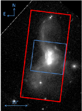
Figure 1: Hubble Space Telescope broad I band image of ESO 148-IG002 taken with the F814w filter on the WFPC2 instrument. The combined field of view of our two WiFeS pointings is overlaid in red and 15" shown for scale. The blue rectangle shows the region with the sufficiently high signal-to-noise for our analyses, and hence only this section is shown in subsequent maps.

2 ESO 148-IG002; Observations, data reduction and line fitting

2.1 ESO 148-IG002 (IRAS 23128-5919)

In appearance, this strongly interacting system is very similar to the nearby NGC 4038/4039 (‘Antennae’) pair. Previous studies of ESO 148-IG002 (with IRAS designation IRAS 23128-5919) show that the galaxy has two nuclei separated by $\sim 4.5$" (Zenner & Lenzen, 1993; Duc et al., 1997), surrounded by bright, possibly star forming knots. The system has two faint tidal tails curling in opposite directions, indicating there was originally two dynamically independent galaxies. Bergvall & Johansson (1985), and Johansson & Bergvall (1988) found LINER and starburst features in the nuclear spectra. They suggested that the nuclear emission-line ratios are consistent with shocks associated with a star burst driven galactic wind. Further studies of infrared mergers by Lípari et al. (2003), agree with this interpretation. Wolf-Rayet (WR) features have also been detected in the southern nucleus by Lípari et al. (2003). Johansson & Bergvall (1988) found a broad intensity enhancement around $\lambda=4650$ Å which they interpret as NIII $\lambda 4641$ and HeII $\lambda 4686$ emission from WR stars of type N. The nucleus of the southern galaxy, although radio quiet, is relatively bright and pointlike, and is suggested to host an active nucleus (Petric et al., 2011; Iwasawa et al., 2011; Bushouse et al., 2002; Stierwalt et al., 2013).

VLT-SINFONI integral field spectroscopic observations have been taken of ESO 138-IG002 by Piqueras López et al. (2012) in the $H$(1.45-1.85$\mu$m) and $K$(1.95-2.45$\mu$m) bands, covering the central $\sim$7-11 kpc. From Pa$\alpha$ equivalent width measurements, they find that the northern nucleus is dominated by star formation, whereas in the southern nucleus, the presence of an AGN is supported by strong compact [SiVI] emission. We compare our kinematic results with the findings of Piqueras López et al. (2012) in Section 4. Rodríguez-Zaurín et al. (2011) use the VLT/VIMOS instrument to study H$\alpha$ in LIRGS and ULIRGS. They are unable to detect ESO 148-IG002’s tidal tails in the ionized gas emission and report that the optical spectrum shows a mix between LINER, Sy2 and HII-like features.

We analyse integral field unit (IFU) data of ESO 148-IG002 to elucidate the relative fraction of the power sources (starburst, AGN, shocks) and nature of shock activity in this galaxy.

2.2 Observations and Data Reduction

Our data for ESO 148-IG002 were taken with the Wide Field Spectrograph (WiFes) at the Mount Stromlo and Siding Springs Observatory 2.3m telescope. WiFeS is a dual beam, image slicing IFU described in detail by Dopita et al. (2007, 2010). Our data consist of separate blue ($\sim$3500-5800 Å) and red ($\sim$5500-7000 Å) spectra with a resolution of R=3000 for the blue and R=7000 for the red. This resolution corresponds to a velocity resolution of 100 km s^-1 at H$\beta$ and 40 km s^-1 at H$\alpha$. Two pointings with WiFeS were taken on July 28 and August 14 and 15 2009, with total exposure times of 3500s and 4000s respectively. The region overlapping the two pointings would therefore have an exposure time of 7500s. The seeing was on average 1.25" for our observations. The WiFeS field of view compared to ESO 148-IG002 is shown in Figure 1. The IFU field consists of 25$\times$ 1" wide slitlets, each of which is 38" long. The spatial pixel is 0.5" along the slitlet axis and 1.0" in the spectral direction. Post reduction, data were binned 2 pixels in the y-direction in order to increase the signal to noise and produce a final resolution of 1"$\times$ 1".
The data were reduced and flux calibrated using the Flux Standard Feige 110 (a white dwarf star) and the WiFeS pipeline. The WiFeS pipeline uses IRAF routines adapted from the Gemini NIFS data reduction package and is briefly described in Dopita et al. (2010). Each observation was reduced into a data cube using the process described in Rich et al. (2011). ESO 148-IG002 was observed using Nod and Shuffle (N$\&$S) mode allowing sky subtraction to be performed using the N$\&$S data. The sky was observed for the same amount of time as the object. The data has bias frames subtracted and any residual bias level is accounted for with a fit to unexposed regions of the detector. The mapping of the slitlets required for spatial calibration is carried out by placing a thin wire in the filter wheel whilst illuminating the slitlet array with a continuum lamp to define the centre of each slitlet. CuAr and NeAr arc lamps are used to wavelength calibrate the blue and red spectra respectively. Observations of a featureless white dwarf taken at similar air mass were used to remove telluric absorption features from the red data cubes.

2.3 Spectral Fitting

To fit and remove stellar continuum from each spectrum, we used an automated fitting routine, UHSPECFIT, which is described in Rupke et al. (2010b) and Rich et al. (2010). The software was based on the fitting routines of Moustakas & Kennicutt (2006), which fits a linear combination of stellar templates to a galaxy spectrum. To fit our relatively high resolution data, we used population synthesis models from González Delgado et al. (2005) as our stellar continuum templates. After the subtraction of the fitted continuum, lines in the resulting emission spectra are fit simultaneously using a one- or two-component Gaussian, depending on the goodness of the fit. The emission line fits are carried out in the same manner as Rich et al. (2011). All spectra were fit using both one- and two-component Gaussians. We adopt the fit with the lowest reduced $\chi^{2}$, however, properties of surrounding spaxels were also used to decide which fit to use. In addition, all fits were checked by eye, to ensure they were reasonable. We determined that $\sim$ 200 spaxels required a two-component Gaussian fit, compared to $\sim$ 140 spaxels whose emission lines were fit with a single component. Each emission line component fit has a corresponding redshift, flux peak and width. The instrumental resolution of 46 km s^-1 FWHM (full width at half maximum) is subtracted in quadrature from the line fit FWHM to compensate for instrumental broadening and converted to a $\sigma$ for the purpose of our analysis. The fitting routines used to fit both the continuum and emission lines made use of the MPFIT package, which performs a least-squares analysis using the Levenberg-Marquardt algorithm (Markwardt, 2009). Example fits are provided in Figure 2, along with an example of a typical spectrum across the entire spectral range.

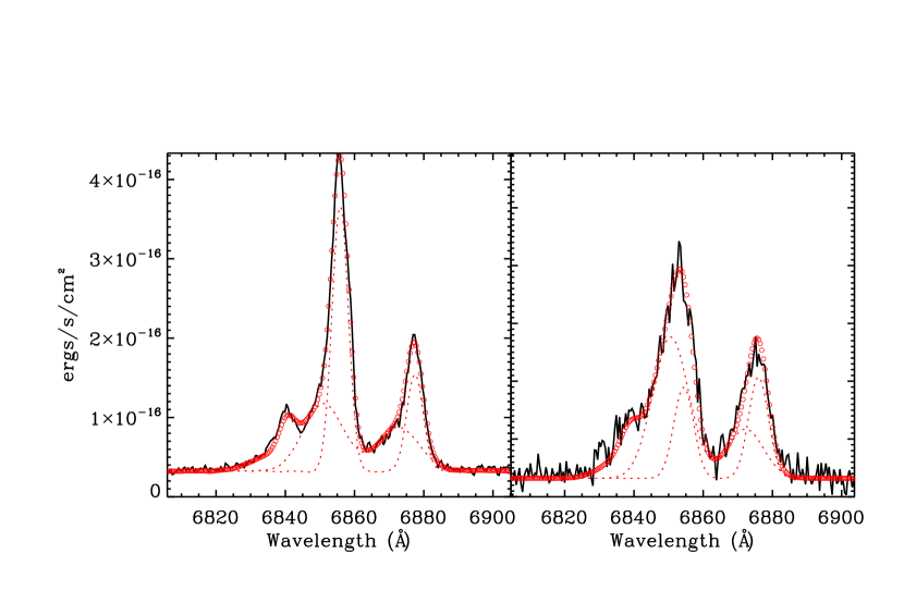
Figure 2: The top two panels show an example of raw data for a single spectrum across the whole spectral range. The bottom panel shows example two-component fits for the H$\alpha$ and [NII] 6583 lines. The flux of the [NII] 6548 component is fixed to the [NII] 6583 flux (ratio 1:3; Osterbrock & Ferland 2006). We do not plot the [NII]6548 line components so the other fitted components can be seen clearly. The right hand spectrum is from the northern nuclear region, whilst the left is from an off-nuclear region east of the southern nucleus. The dashed red lines show the two Gaussian functions which together give the overall emission fit. The raw data are in black and the continuum plus emission fit is in red. Both components are often well defined in one emission line but not in another. Where the amplitude of an individual component is not more than five standard deviations above the noise, it is not considered in subsequent analysis.

Errors in the parameters used in fitting Gaussian functions to the emission lines are calculated by the MPFIT package, using the variance spectrum as input. To analyse multiple component fits, we minimise the $\chi^{2}$ for all lines simultaneously. As such all lines ([OII]3726, H$\beta$, [OIII]4959, [OIII]5007, [OI]6300, [NII]6548, H$\alpha$, [NII]6583, [SII] 6716. [SII]6731) have the same velocity and velocity dispersion. Assuming that all the gas contained within a given spaxel is undergoing the same processes, we would expect each emission line in the spectrum to have the same velocity dispersion. By fitting all lines simultaneously, we decrease the overall uncertainty in the velocity dispersion and maintain the ability utilise the multiple component fits.

As our analysis of this kinematically complex system relies on a careful decomposition of multiple velocity dispersions, it is crucial that more than one Gaussian can be used in the emission line fit.

3 Emission line gas properties

3.1 Line Ratio Maps

We examine the maps of the ratios of the total flux of [NII]$\lambda$6583, [SII]$\lambda\lambda$6716,6731 and [OI]$\lambda$6300 to H$\alpha$ in Figure 3 as a first step towards understanding the processes at work in ESO 148-IG002. Where two Gaussians are used to fit an individual emission line, the total flux is taken to be the sum of the two component fluxes. These ratios are sensitive to metallicity as well as ionization parameter and have the advantage that they do not require reddening corrections. Line ratio values corresponding to each spaxel are also plotted on standard diagnostic diagrams in Figure 4. In general, the weaker the line ratio, the greater the contribution of pure star formation to the ionizing spectrum (Kewley et al., 2006). In Figure 3 we also show the ratio of [OIII]$\lambda$5007 to H$\beta$, used in all diagnostic diagrams of Figure 4. We represent the errors in the line ratio values by mapping the uncertainty in each spaxel on a logarithmic scale.

The [NII]/H$\alpha$ ratio is sensitive to metallicity (Kewley & Dopita, 2002; Denicoló et al., 2002; Pettini & Pagel, 2004; Kewley & Ellison, 2008). The higher [NII]/H$\alpha$ ratio in the southern corner of the galaxy could thus correspond to a higher metallicity clump, however the AGN in the southern nucleus (bottom white cross in Figure 3) may also contribute to the [NII]/H$\alpha$ ratio. The other two ratios, [SII]/H$\alpha$ and [OI]/H$\alpha$, are more sensitive to a hard radiation field from AGN or shocks. Higher ratios in the outer regions, such as in these two maps, usually correspond to shocked regions (e.g. Rich et al. 2010; Monreal-Ibero et al. 2010; Sharp & Bland-Hawthorn 2010; Rich et al. 2011. However, in this case there are only $\sim$2 spaxels detected in the outer regions with elevated [SII]/H$\alpha$ and [OI]/H$\alpha$ ratios, so we cannot conclude whether shocks are affecting the area.

                

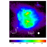
(a) HST

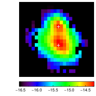
(b) H$\alpha$

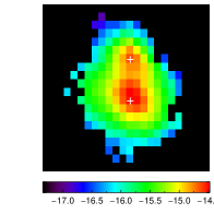
(c) [NII]

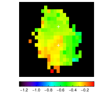
(d) [NII]/H$\alpha$

(e) HST

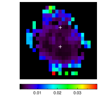
(f) H$\alpha$ error

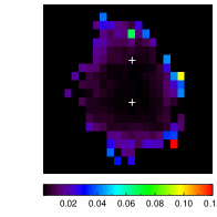
(g) [NII] error

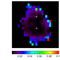
(h) [NII]/H$\alpha$ error

(i) HST

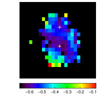
(j) [SII]/H$\alpha$

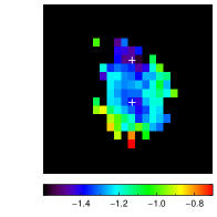
(k) [OI]/H$\alpha$

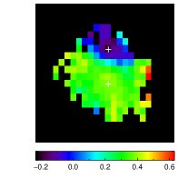
(l) [OIII]/H$\beta$

(m) HST

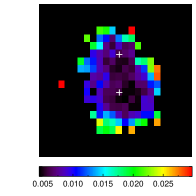
(n) [SII]/H$\alpha$ error

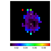
(o) [OI]/H$\alpha$ error

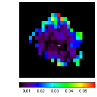
(p) [OIII]/H$\beta$ error

Figure 3: Emission line ratio maps using total fluxes (the sum of both Gaussians if a double fit is made). All scale bars show the log of the value indicated by the captions. The top images show the log of the total emission of [NII] and H$\alpha$ (in units of ergs s^-1 cm^-2 Å^-1) of ESO 148-IG002, and the ratio of the two. In both the H$\alpha$ and [NII] maps, two peaks in the emission can be seen. This most likely corresponds to the two nuclei from the original galaxies (as determined by the peaks in the HST image), shown by white crosses on the maps. Underneath the images their corresponding relative error maps are also shown on a logarithmic scale. Images (j), (k), and (l) are the line ratio maps corresponding to the diagnostic diagrams for log([SII]/H$\alpha$), log([OI]/H$\alpha$) and log([OIII]/H$\beta$). The left most panels are the HST image of ESO 148-IG002 shown in Figure 1, with the same dimensions and orientation as the other maps, for reference. The white circle on the bottom right corner of the HST image is an estimate of the seeing for our WiFeS observations.

3.2 Diagnostic Diagrams

To better understand the contributing power sources in this galaxy, we use line ratio diagnostic diagrams. Diagnostics using the [NII]/H$\alpha$, [SII]/H$\alpha$ and [OI]/H$\alpha$ against [OIII]/H$\beta$ ratios were first employed by Baldwin et al. (1981) and Veilleux & Osterbrock (1987) to distinguish the likely ionizing source of emission line gas in galaxies. Kewley et al. (2001) used a combination of stellar population synthesis models and self-consistent photoionization models to determine a theoretical “maximum starburst line” on the diagrams which indicates the theoretical upper limit given by pure stellar photoionization models. The diagrams have been subsequently updated by Kauffmann et al. (2003) and Kewley et al. (2006) to include empirical lines dividing pure star-forming from Seyfert-HII composite galaxies and Seyferts from LINER galaxies respectively.

We show the diagnostic diagrams for ESO 148-IG002 in Figure 4. We include the emission line fluxes from each spaxel with $S/N>5$ in all relevant lines. This procedure allows us to classify the dominant energy source in each spaxel. In all three diagrams the lower left hand section of the plot traces photoionization by HII regions. The solid curve traces the upper theoretical limit to the pure HII region contribution measured by Kewley et al. (2001). The observed dashed line in the [NII] diagnostic provides an empirical upper limit to the pure HII region sequence of Sloan Digital Sky Survey galaxies measured by Kauffmann et al. (2003). The region lying between these two lines represents objects with a composite spectrum which is a mix of HII region emission and a stronger ionizing source. LINER-like emission lies to the right-hand side of the diagrams whilst contribution from a Seyfert AGN will push the spaxels upwards on all three diagrams. If the galaxy is influenced by shocks, the line ratios can be moved towards the LINER region (Rich et al., 2010, 2011). From the [NII] diagnostic plot it is clear that there are very few purely star forming regions in this galaxy.

The large number of SDSS galaxies ($\sim$45,000), allowed Kewley et al. (2006) to separate two clear branches on the [SII]/H$\alpha$ and [OI]/H$\alpha$ diagnostic diagrams, empirically deriving a boundary between Seyfert 2s and LINERs seen as the dashed lines on these diagrams. LINERs have a harder ionizing radiation field and lower ionization parameter than Seyfert galaxies, making the [SII]/H$\alpha$ and [OI]/H$\alpha$ diagrams ideal for separating Seyferts and LINERS. The [SII] and [OI] emission lines are produced in the partially ionized zone at the edge of the nebula. For hard radiation fields, this zone is large and extended. The [NII]/H$\alpha$ ratio only weakly depends on the hardness of the radiation field, is much more dependent on the metallicity of the nebular gas and thus cannot be used to separate Seyfert and LINER galaxies. The [SII] and [OI] diagnostic diagrams in Figure 4 indicate that the composite HII regions seen in the [NII] diagram could be influenced by AGN activity as the spaxels are spread upwards towards the Seyfert 2 branch.

ESO 148-IG002 has a bimodal distribution of [OIII]/H$\beta$ line ratios, which we have visually separated in the top panel of Figure 4. The location of the spaxels with high and low [OIII]/H$\beta$ ratios on the BPT diagram, combined with their physical location in the galaxy, could suggest that the northern nucleus has a higher metallicity than the southern nucleus.

 

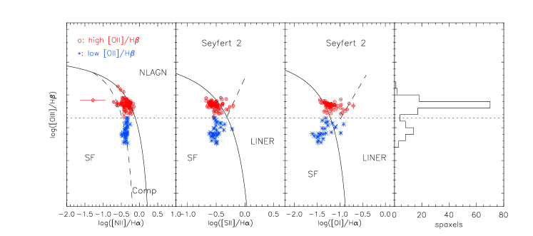
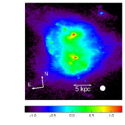
(a) HST

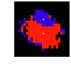
(b) Location of spaxels

Figure 4: Emission line ratio diagnostic diagrams of each individual fitted emission line. Here total fluxes for each line are used (as in Figure 3). Black solid curves form an upper limit for star-forming galaxies as derived by Kewley et al. (2001). The dashed line on the [NII] diagram is the empirical Kauffmann et al. (2003) boundary below which galaxies are classified as star-forming. The dashed lines on the [SII] and [OI] diagrams were derived by Kewley et al. (2006) to empirically separate Seyfert 2 galaxies and LINERs. In the leftmost panel, NLAGN represents narrow emission-line AGN (Seyfert 2 plus LINERs); Comp represents starburst-AGN composites. We apply a minimum S/N cut of 5 in every diagnostic line. Typical errors are 0.009 dex for log([NII]/H$\alpha$) and log([SII]/H$\alpha$), 0.016 dex for log([OI]/H$\alpha$) and 0.012 for log([OIII]/H$\beta$). The spaxels in each diagram reflect a mix of ionization sources. The spaxels are distributed in two clumps in [OIII]/H$\beta$ as shown in the histogram of the top right panel. The division between the two clumps is shown across the top panel by the dotted line, marking the minimum in the bimodal [OIII]/H$\beta$ distribution. The points are also colour coded based on this division. The spatial position of the clumps are shown in the bottom right panel, with the red and blue colors matching those from the BPT diagram. This could indicate that gas from the northern nucleus (blue) has a higher metallicity.

4 Kinematic Properties

The power source of the emission line ratios is unclear from the diagnostic diagrams alone. In this section we try to better understand the dynamics as well as the different power sources of ESO 148-IG002. Here we make most use of the two Gaussian component fits. As all emission lines in a spectrum were fit simultaneously with one or two Gaussian components, all lines per spaxel have the same velocities, and velocity dispersions, which are used in this section. In data with high spectral resolution, one can analyse the distribution of velocity dispersions to separate the galaxy’s ionizing sources.

4.1 Velocity Dispersion

Velocity dispersion, $\sigma$, is the result of the superposition of many line profiles, each of which has been Doppler shifted and broadened because of the gas motions within the galaxy. The velocity dispersions used for our analysis have had the instrumental resolution ($\sim$ 40 km s^-1 FWHM in the red) subtracted in quadrature to account for instrumental broadening. In a complex galaxy such as ESO 148-IG 002, a large proportion of the gas may be affected by more than one source of ionization. In this section we focus on the velocity dispersion of individual emission line components, determined from the two component fits, as a useful way to probe the processes influencing each spaxel. HII regions correspond to a low velocity dispersion, typically of a few tens of km s^-1 (Epinat et al., 2010), while slow shocks associated with galactic winds have velocity dispersions $\ga 100$ km s^-1(Rich et al., 2010, 2011), and the presence of an AGN can produce even broader lines (Wilson & Heckman, 1985). In Figure 5 we show the velocity dispersion distribution from every component fit by our routine with S/N$>$5. The spectrum from every spaxel was fit with either one or two Gaussian curves with each emission line in a spectrum having the same fixed dispersion values (one or two depending how many components were needed), and all components (for every spaxel) are shown.

We establish a cutoff of $\sigma=155$ km s^-1 between the low-$\sigma$ HII region emission and higher $\sigma$ emission by shocks and/or AGN, as there is a local minimum in the velocity dispersion distribution at this value (Figure 5). The choice of appropriate cutoffs was also influenced by the velocity dispersion maps, shown in Figure 6. The fact that the different components occupy different regions indicates that they may be influenced by different phenomena. In some cases a spaxel has more than one component in the same velocity dispersion bin. In this case, to create the velocity dispersion maps, the $\sigma$ values were averaged (weighted by the component’s H$\alpha$ flux) over the two components within the same bin. The high velocity dispersion gas is located to the South of the system, where the AGN lies. However, the peak velocity dispersion is offset from the nucleus. This is consistent with the idea that the high velocity dispersion gas is powered in part by an AGN. As shocks tend to correspond to a larger velocity dispersion than that seen on the outskirts of this galaxy, it is unlikely that shocks are contributing significantly to the emission spectrum.

Figure 5: Velocity dispersion distribution from every individual Gaussian component fit. The distribution has a peak around $\sim$ 100 km s^-1. Pure star-forming regions have velocity dispersions of $\sim 40$ km s^-1 (Epinat et al., 2010). Therefore it is likely that spaxels with velocity dispersions less than the local minimum at $\sigma<155$ km s^-1 are likely to be dominated by star formation, but also have contribution from shock or AGN. The extended distribution out to higher velocity dispersions could represent an increasing contribution from AGN activity.

  

(a) HST

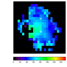
(b) $\sigma<155$ km s^-1

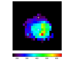
(c) $\sigma>155$ km s^-1

Figure 6: Velocity dispersions in km s^-1 of the two components, with grouping determined by the cut off. Left to right corresponds to increasing velocity dispersion. For spatial comparison the HST image has been aligned and placed in the leftmost panel. Where a spaxel contains two components fit which fall in the same velocity dispersion bin, we show a flux weighted average. Spaxels which do not appear in the $\sigma>155$ km s^-1 figure are the cases where either only one component is fit, and that component is narrow, or two components are fit and both are narrow. The low velocity dispersion gas is extended over the whole galaxy, whereas the high velocity dispersion gas is only found in the southern region.

4.2 Velocity Maps

Using the separate Gaussian components we are able to calculate the recessional velocity for each of the two velocity dispersion groups. We adopted a systemic redshift of z=0.04460 (Lauberts & Valentijn, 1989). The velocity maps are shown in Figure 7. A velocity shear can be seen in the map of the second, broader component ( $\sigma>155$ km s ^-1), centred over the southern nucleus. The low velocity dispersion component, which likely corresponds to star forming regions based on its velocity dispersion, does not show rotation. However, it is possible that this component could be a face-on rotating structure, in which case we would not see a velocity shear.

Studying P$\alpha$ in ESO 148-IG002, Piqueras López et al. (2012) similarly find low velocity dispersions ($\sim$65 km s^-1) in the northern nucleus and high velocity dispersion ($\sim$190 km s^-1) in the southern nucleus. They observe red and blue wings in the P$\alpha$ and H₂1-OS(1) line profiles which they suggested forms a cone-like structure, centered on the AGN and extending $\sim 3-4$ kpc north-east and south-west. Piqueras López et al. (2012) also report a velocity gradient of $\Delta v\sim$140 km s^-1 around the northern nucleus in a north-south direction, a feature which can also be seen in our Figure 6b. We show, by decomposing emission lines into two Gaussian components, that the velocity shear observed in the south, extends out to $\sim 15$ kpc in the optical.

We propose two possible explanations for the velocity and velocity dispersion fields of ESO 148-IG002. Firstly, the rotating component seen to the south, could be the disk of the progenitor spiral, containing an AGN. Due to the large spatial coverage of this rotating component ($\sim 15$ kpc) it is difficult to compare this component to other studies such as U et al. (2013) who observe rotating gas $<1$ kpc from an AGN. However, larger samples of (U)LIRGs (Medling et al., 2014) do see evidence of both small nuclear disks (r $\sim$ few hundred pc) and larger disks (r $>$ 1 kpc), which they also interpret as the progenitor galactic disk. The velocity broadening is likely due to the presence of the AGN. However, beam smearing could also cause an increased velocity dispersion. [OIII] is commonly used to measure the size of narrow-line regions (NLRs) in AGNs, typically giving extents of 1-5 kpc (Bennert et al., 2006; Davies et al., 2014). It is unlikely that the AGN at the center of the southern nucleus is able to cause the high line ratios observed ([OIII]/H$\beta$) at 15 kpc without help from star formation or shocks.

Secondly, the velocity shear, which was previously interpreted as rotation, could represent an AGN bipolar outflow, similar to that seen in Davis et al. (2012) and suggested in Piqueras López et al. (2012). Harrison et al. (2012) find broad [OIII] emission lines ($\sigma=$ 300-600 kms^-1) in high-redshift(z=1.4-3.4) galaxies containing AGN. The broad emission line regions extend across 4-15 kpc and have high velocity offsets from the systemic redshift ($\approx$ 850 km$s^{-1}$) and are attributed to galaxy-scale AGN-driven winds. ESO 148-IG002’s broad velocity dispersion gas has a more modest velocity offset ($\sim$350 km s^-1) than the outflows in the Harrison et al. (2012) sample, however, the high velocity dispersion, large spatial extent, and velocity shear are consistent with the AGN-driven outflow scenario.

By comparing the ionized gas kinematics with the stellar velocity field, Davis et al. (2012) was able to conclude that their high velocity dispersion component was due to shocked outflow, as the axis of the gas’ velocity gradient was offset from the stellar rotation axis. Information on the stellar kinematics of ESO 148-IG002’s could help differentiate between the two scenarios proposed here.

For the purposes of clarity, we refer to the kinematically distinct broad component as “rotating” in subsequent analysis, though the reader should remember that its coherent structure may either be rotation or outflows.

Fitting a disk model to the rotating component could also help decide whether the velocity shear is due to rotation or outflow. Disk fitting and kinemetry analysis (Krajnović et al., 2006) will be subject of future work, with a larger sample of galaxies, allowing us to better understand the kinematic properties of complex galaxy systems.

  

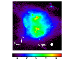
(a) HST

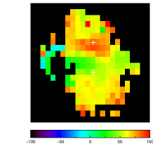
(b) Velocity(km s^-1): $\sigma<155$ km s^-1

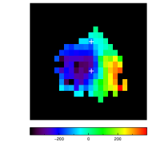
(c) Velocity(km s^-1): $\sigma>155$ km s^-1

Figure 7: Maps of velocity for the two components determined by our cutoff. From left to right the images correspond to the velocity of spaxels with velocity dispersions of: $\sigma<155$ km s^-1 and $\sigma>155$ km s^-1. Where a spaxel contains two components fit which fall in the same velocity dispersion bin, we show a flux weighted average velocity. For spatial comparison the HST image has been aligned and placed in the leftmost panel. The high velocity dispersion gas located to the south shows a velocity shear which we interpret either rotation or outflow.

5 Analysis

In the previous section we separated the emission line fluxes into two components, one with velocity dispersions $\sigma<155$ km s^-1, and the other with velocity dispersions higher than $\sigma>155$ km s^-1. The distribution of flux into the two components is illustrated in Figure 8, which maps the H$\alpha$ flux in the low and high velocity dispersion components. Low velocity dispersion gas is present throughout the system, whereas the high velocity dispersion gas is centred on the southern nucleus, where the AGN lies. In this section we use the emission line ratios of the separate components to analyse two potentially distinct power sources.

   

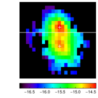
(a) H$\alpha$: $\sigma<155$km/s

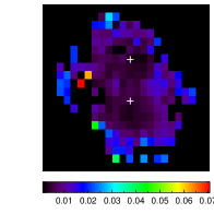
(b) H$\alpha$ error: $\sigma<155$km/s

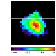
(c) H$\alpha$: $\sigma>155$km/s

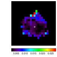
(d) H$\alpha$ error: $\sigma>155$km/s

Figure 8: Maps of the log of the H$\alpha$ emission (in units of ergs s^-1 cm^-2 Å^-1) of the two Gaussian components determined by our velocity dispersion cutoff and their corresponding uncertainty maps. From left to right the images correspond to the velocity of spaxels with velocity dispersions of: $\sigma<155$ km s^-1 and $\sigma>155$ km $s^{-1}$. The distribution of the two components match with the HST nuclei with the southern component peak consistent with the AGN position. Horizontal white lines on the flux maps mark the division between the north and south nuclei from which we calculate distances in Section 5.2.

5.1 Diagnostic Diagrams

In Figure 9 the spaxels on the optical diagnostic diagrams are colour coded by velocity dispersion. Line emission from each Gaussian component of every spectrum with $S/N>5$ is considered here. If the two different colours occupy separate positions on the diagnostic diagrams, then this separation would imply that different ionizing sources are responsible for each velocity component. Separating the emission lines in a spaxel in up to two components results in a greater number of data points than shown in Figure 4. When two or more processes are working to power the emission spectrum of the gas, using a line’s total flux for analysis, as in Figure 4, works to average the effects that the different processes may have. Separating the flux into two separate components, based on their velocity dispersion, allows us to analyse two potentially different power sources. There are fewer high velocity dispersion components present in the [SII]/H$\alpha$ diagnostic diagram and only one in the [OI]/H$\alpha$ diagram. The lack of high velocity dispersion spaxels is a result of applying a signal to noise cut on each component fit.

Figure 9 shows that the broad component is dominated by spaxels in the Seyfert and composite region of the diagnostic diagram, while a larger fraction of the narrow component lies in the HII-region portion of the diagnostic diagram. The low velocity dispersion components spread upwards predominantly to the AGN regions in both the [SII] and [OI] diagnostic diagrams indicating that even the low velocity dispersion gas could be affected by the AGN and/or shocks.

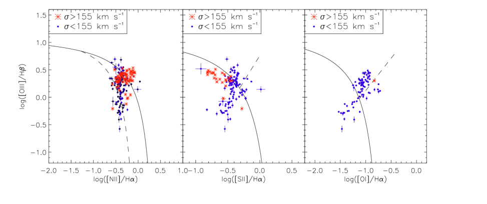
Figure 9: As Figure 4, but with separate Gaussian components color-coded based on their velocity dispersions. Separating the emission lines in a spaxel in up to two components results in a greater number of data points than shown in Figure 4. Spaxels with $\sigma$ less than 155 km s ^-1 are plotted in blue, and the highest velocity dispersions, $\sigma$ greater than 155 km s^-1 are coloured red. Every line used has S/N $>5$. The broad components are mostly in the Seyfert region on these diagrams and the narrow component spaxels are spread from the star forming region upwards, indicating a larger contribution from star formation in the low velocity dispersion gas.

5.2 Metallicity Gradient

To find the metallicity (given as 12+log(O/H)) of ESO 148-IG002, we use the method of Kobulnicky & Kewley (2004), which uses the stellar evolution and photoionization grids from Kewley & Dopita (2002) to produce an (updated) analytic prescription for estimating oxygen abundances using the traditional strong emission line ratio $R_{23}$, where $R_{23}=([OII]\lambda 3727/[OIII]\lambda\lambda 4959,5007)/H\beta$. The $R_{23}$ calibration is sensitive to the ionization state of the gas, particularly for low metallicities. The ionization state of the gas is characterised by the ionization parameter (the number of hydrogen-ionizing photons passing through a unit area per second, divided by the hydrogen density of the gas), which is typically derived using the [OIII]/[OII] ratio. However, this ratio is also sensitive to metallicity, so Kobulnicky & Kewley (2004) suggest an iterative approach to derive a consistent ionization and metallicity solution. We first determine whether the spaxels lie on the upper or lower $R_{23}$ branch using the [NII]/[OII] ratio and calculate an initial ionization parameter assuming a nominal lower branch [12+log(O/H)=8.2] or upper branch [12+log(O/H)=8.7] metallicity using:

$$\log(q)=(32.81\!-1.153y^{2}\!+[12+\log(O/H)](-3.396$$

$$-0.025y+0.1444y^{2})(4.603-0.3119y-0.163y^{2}$$

$$+[12+\log(O/H)](-0.48+0.0271y+0.02037y^{2}))^{-1}$$ (1)

where $y=\log([OIII]\lambda 5007/[OII]\lambda 3727)$. A spaxel is determined to lie on the lower $R_{23}$ branch if $\log([NII]/[OII])<-1.2$, and on the upper branch if $\log([NII]/[OII])>-1.2$. The initial ionization parameter is then used to derive a metallicity estimate, using

$$12+\log(O/H)_{lower}=9.40+4.65x-3.17x^{2}$$

$$\qquad\quad-\log(q)(0.272+0.547x-0.513x^{2})$$ (2)

where $x=\log(R_{23}),$ if the spaxel lies on the lower branch, and

$$12+\log(O/H)_{upper}=9.72-0.777x-0.951x^{2}-0.072x^{3}$$

$$\quad-0.811x^{4}-\log(q)(0.0737-0.0713x-0.141x^{2}$$

$$\qquad+0.0373x^{3}-0.058x^{4}),$$ (3)

if the spaxel lies on the upper branch. Equations 1 and 2 (or 3) are iterated until $12+\log(O/H)$ converges. To find the metallicity of spaxels dominated by star-formation, emission line fluxes from the low velocity dispersion component, with S/N greater than 5 in all relevant lines, lying to the left of the empirical line from Kauffmann et al. (2003) (seen in Figure 9) were used, and an average metallicity of $log(\frac{O}{H})+12=9.09$ ($\pm 0.03$ dex) was obtained. Metallicity as a function of radius is plotted in Figure 10. As there are two nuclei in ESO 148-IG002, we have separated the spaxels into two groups, a northern and southern, using the spatial cut-off given by the boundary of the rotating broad component gas (Figure 8). Spaxels belonging to the northern nucleus were determined to be spaxels north of the broad component seen in Section 4.2, and as such the distance to these spaxels is given from the northern nucleus. Distances to spaxels south of this spatial boundary are calculated from the position of the southern nucleus. The gas metallicity of the star forming regions remains constant around the mean value as a function of nuclear distance, with a scatter of $\sim 0.2$ dex.

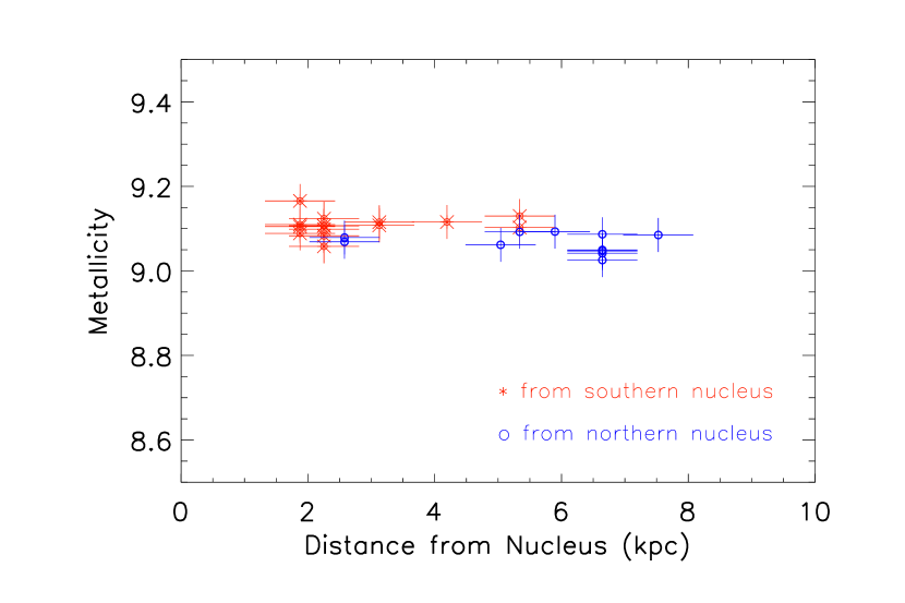
Figure 10: Metallicity versus distance from corresponding nucleus. Metallicities in red lie to the north of the system. For these metallicities, the distance has been measured from the northern nucleus. Blue metallicities lie to the south of the galaxy and the distance to them is calculated from the southern nucleus. Uncertainties in the distance from the nucleus are derived from the average seeing of our observations. No gradient in the metallicity as a function of radius is evident.

Normal spiral galaxies have negative metallicity gradients consistent with central enrichment from generations of star formation (Henry & Worthey, 1999). Figure 10 indicates that ESO 148-IG002 has a flat metallicity gradient. Flat metallicity gradients can be produced by merger-induced gas inflows (Kewley et al., 2010; Rupke et al., 2010; Torrey et al., 2012). The gradient in ESO 148-IG002 is flatter than any mergers in Kewley et al. (2010) and may indicate very recent gas infall.

5.3 AGN, Shock and HII models

To determine the effects (if any) of shock excitation, we employ slow shock models, which were introduced and described in Farage et al. (2010) and Rich et al. (2010). Slow shock models with velocities consistent with our observed line widths, (100-200 km s^-1) were generated using an updated version of Mappings III code, originally introduced in Sutherland & Dopita (1993). We also compare HII region models generated using Starburst99 (Leitherer et al., 1999) and Mappings III (Kewley et al., 2001; Levesque et al., 2010). We show mixing sequences of star formation and shock excitation in Figure 11 for a metallicity of 8.69 (solar), calculated by varying the fractional contribution of the HII and shock models on the line ratios. Higher metallicity models would lie lower on the diagrams and are inconsistent with the position of ESO 148-IG002. Not all spaxels are covered by the shock-mixing models shown in Figure 11. Therefore although some spaxels may be influenced by shocks, it is likely that (a mixing between star formation and) another phenomenon is causing the high line ratios seen.

We also employ a dusty, radiation pressure-dominated photoionization model first introduced in Dopita et al. (2002), and updated in Groves et al. (2004). These models provide a self consistent explanation for the emission from narrow-line regions of AGN. From the family of models available, we explored those with hydrogen number density of $10^{3}$ cm^-3 and a metallicity of 2Z_⊙ to match the properties of ESO 148-IG002. A simple power law represents the spectral energy ($\nu$) distribution of the ionizing source, with

$$F_{\nu}\propto\nu^{\alpha},\nu_{min}<\nu<\nu_{max}.$$

and $\nu_{min}=$ 5eV and $\nu_{max}=$ 1000eV. Four values of the power-law index, $\alpha$ are shown in Figure 12; -1.2,-1.4,-1.7, and -2.0 as these indices encompass the range of indices seen in AGN locally (Groves et al., 2004). The ionization parameter, log $U_{0}$ in the model shown varies between 0.0 and -2.3 dex. We also construct a starburst-AGN mixing sequence, by varying the fractional contribution of the HII and AGN models on the line ratios in linear space. The mixing sequence shown in Figure 12 results from applying this method on a single pure HII region and pure twice solar metallicity AGN region indicating changes in the fraction of starburst to AGN of 10 $\%$ in linear space.

Neither model encompasses all spaxels from ESO 148-IG002. Recall from Figure 9 that almost all of the spaxels on the [OI] diagnostic are of lower velocity dispersion. Low velocity dispersion spaxels lie on both the shocked mixing sequence and the AGN mixing sequence. Spaxels in the higher velocity dispersion group are closer to the AGN models, which indicates that this high $\sigma$ component is influenced more strongly by the AGN in the southern nucleus, over which those spaxels lie.

To determine whether the starburst-AGN or starburst-shock models better describes our emission line data, we perform the statistical Kolmogorov-Smirnov (KS) test. The KS test is a nonparametric test of the equality of two continuous distributions and can be used to determine the likelihood that a sample distribution was drawn from reference distribution (one-sided KS test), or to compare two sample distributions (two-sided KS test). We compare the values of ESO 148-IG002’s [OIII]/H$\beta$ and [SII]/H$\alpha$ ratios with the values estimated from the above mixing sequences using a two-dimensional, two-sided KS test. Although the KS test is only strictly defined for one dimensional probability distributions, Press et al. (2002) describes how an analogous test can be designed and implemented when the distribution depends on two variables. We use the combination of [OIII]/H$\beta$ and [SII]/H$\alpha$ ratios for this test as the [SII]/H$\alpha$ ratio is more sensitive to shocks than [NII]/H$\alpha$, and is of higher signal to noise in our data than the [OI]/H$\alpha$. Table 1. lists the $p$ values calculated using the two sided KS test. A $p$ value close to one means that there is a high probability that the two samples originated from the same parent distribution. We find that gas with $\sigma<155$ km s^-1 can be better described by the AGN mixing sequence, than with the shock mixing sequence used, with $p$ values 0.73 and 0.59 respectively. The high velocity dispersion gas with $\sigma>155$ km s^-1 is also better described by our AGN mixing model, with $p$=0.63 as compared with $p$=0.48 for the shock mixing model. As previous studies have indicated the presence of an AGN in the southern nucleus as well as star formation, it is not surprising that both the line ratios and velocity dispersions of ESO 148-IG02 show a mixture of star formation and AGN activity. Both the low and high velocity dispersion components are better described by the model AGN mixing sequence than the shock mixing sequence. It is likely that the high velocity dispersion component traces gas strongly influenced by the AGN, whilst the low velocity dispersion gas is more strongly influenced by star formation with AGN activity having a small effect.

Figure 11 suggests that more theoretical work is needed to accurately model the [SII] emission-line fluxes in merging galaxies. Unlike the [NII]/Ha and [OI]/Ha mixing sequences, the [SII]/Ha line ratios are not well-fit by the mixing sequence. The difficulty in modeling the [SII]/Ha lines in galaxies is well known (e.g., Levesque et al. 2010), and has been attributed to the theoretical shape of the EUV radiation field.

$p$ value	shock	AGN
$\sigma<155km/s$	0.587	0.729
$\sigma>155km/s$	0.481	0.628

Table 1: The results of performing the KS test which compared the ratios of [SII]/H$\alpha$ and [OIII]/H$\beta$ for each spaxel, with a model star forming-shock mixing sequence, and a model star forming- AGN mixing sequence. Values of $p$ closer to one imply that the underlying distributions are more likely the same, i.e that the model is preferred. We find that the AGN mixing sequence better describes our data than the shock mixing sequence.

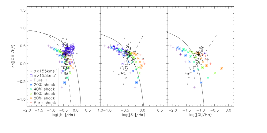
Figure 11: As Figure 9, but with spaxels corresponding to the high velocity dispersion gas in blue, and the low velocity dispersion gas in black. Overplotted are HII region and shock models, with varying ionization parameter (6.5-8.0), and shock speed (100-200 km s^-1) for solar metallicity (8.69). In between, we show a mixing sequence from pure HII region to pure shock excitation. Increasing shock velocity or decreasing ionization parameter decreases the [OIII]/H$\beta$ ratio and increases the other ratios. The shock mixing models do cover some of the data but are unable to explain all of ESO 148-IG002’s line ratios. Parts of the shock mixing models fall on the same region as AGN mixing models (Figure 12), as they both start from the HII region model. Thus even though some spaxels are consistent with our shock models, we can not conclude that the gas is shocked.

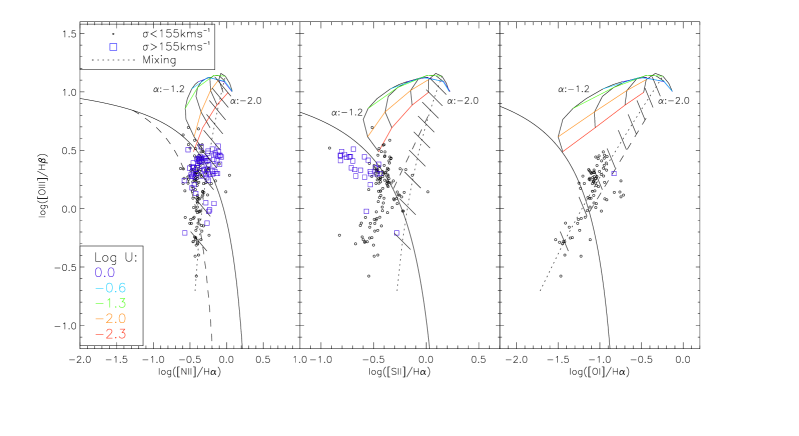
Figure 12: As Figure 9, but with spaxels corresponding to the high velocity dispersion gas in blue, and the low velocity dispersion gas in black. Included are the twice solar metallicity AGN models from Groves et al. (2004). The power-law index $\alpha$ values (black grid lines) represented are -1.2, -1.4, -1.7, and -2.0. Ionization parameter ($\log U_{0}$) values represented include 0.0, -0.6, -1.3, -2.0, and -2.3. A mixing sequence between a pure HII region and a pure twice solar metallicity AGN region is created, with each line representing a change in the fraction of starburst to AGN of 10 $\%$ in linear space (dotted line). A combination of AGN and HII region models better describe our line ratios than the shock models of Figure 11.

6 Discussion

Observations by Rich et al. (2012) and Kewley et al. (2010), and simulations (Rupke et al., 2010) show that there is a strong relationship between metallicity gradients and the gas dynamics in galaxy interactions and mergers. As a merger progresses the metallicity gradient is flattened. This flattening reflects the effects of gas redistribution over the disks, including less enriched gas being torqued towards the centre and the growth of tidal tails that carry metals out to large radius. In the previous section we found the metallicity gradient of ESO 148-IG002 is flatter than any of the sample galaxies in Kewley et al. (2010). Based on our analysis, we present the following picture of ESO 148-IG002:

Gas from the northern galaxy has been spread out across the whole system as a result of the merger. This constitutes the low velocity dispersion component ($\sigma<155$km s^-1) which covers ESO 148-IG002. This area is most likely to be dominated by star formation as indicated from the optical diagnostic line ratios. The mixing of the gas due to the gravitational forces acting between the two galaxies is likely to be responsible for the flat metallicity gradient observed. The southern galaxy seems to have remained dynamically distinct from the northern galaxy, either maintaining a rotation that is not seen in the gas with lower velocity dispersion, or being the result of an AGN-driven outflow. The southern nucleus contains an AGN which is the most likely cause for the high velocity dispersion in the surrounding gas ($\sigma>155$km s ^-1). The few spaxels that lie near the southern nucleus have velocity dispersions of $\sim$600 km s^-1, consistent with an AGN. It is not possible to entirely rule out shocks from the galaxy. From the line ratios it is possible that at least some of the galaxy is influenced by shock excitation.
Considering this interesting scenario and the flat metallicity gradient of the galaxy, we suggest that we are observing ESO 148-IG002 in the middle of (or just after) major gas rearrangement related to its merger, which makes it an exciting candidate for future studies of star formation and AGN fuelling.

7 Conclusion

Using WiFeS wide integral field spectroscopy of the ULIRG ESO 148-IG 02 we found that:

$\bullet$ The distribution of gas velocity dispersion is bimodal, indicating a combination of power sources.
$\bullet$ The emission line ratios indicate composite starburst and AGN activity, with a starburst-AGN mixing model better able to explain the data than a starburst-shock mixing model (AGN mixing model produced $p$ values of 0.73 and 0.63 for the low and high velocity dispersion gas respectively, compared to $p$ values of 0.59 and 0.48 for shock mixing models when tested using the KS statistic).
$\bullet$ The HII regions, dominated by star formation and given by the lower-$\sigma$ component, have a mean metallicity of 9.09$\pm$0.03.
$\bullet$ The galaxy has a flat metallicity gradient as a result of the merging process.
$\bullet$ The high $\sigma$ gas associated with the southern nucleus has a coherent velocity pattern which could either be rotation or an AGN-driven outflow.

It is possible that we have caught this merger as the gas from the northern galaxy is being mixed throughout the two galaxies. If this is the case, we have shown that it is possible to disentangle two galaxies in a merging system based entirely on its kinematic analysis.
ESO 148-IG002 provides an exciting test bed for future work on the potential triggering of starbursts and AGN by merger induced gas flows.

ACKNOWLEDGMENTS

L.K. gratefully acknowledges the support of an ARC Future Fellowship and ARC Discovery Project grant DP130103925. We would like to thank A. Medling for discussing the interpretation of the kinematic components with us. This research has made use of NASA’s Astrophysics Data System Bibliographic Services and the NASA/IPAC Extragalactic Database (NED). The authors are very grateful to two anonymous referees whose comments and suggestions greatly improved the clarity of this paper.

99

References

- Armus et al. (1989) Armus, L., Heckman, T. M., & Miley, G. K. 1989, ApJ, 347, 727
- Armus et al. (2009) Armus, L., Mazzarella, J. M., Evans, A. S., et al. 2009, PASP, 121, 559
- Baldwin et al. (1981) Baldwin, J. A., Phillips, M. M., & Terlevich, R. 1981, PASP, 93, 5
- Barnes & Hernquist (1996) Barnes, J. E. & Hernquist, L. 1996, ApJ, 471, 115
- Bennert et al. (2006) Bennert, N., Jungwiert, B., Komossa, S., Haas, M., & Chini, R. 2006, A&A, 456, 953
- Bergvall & Johansson (1985) Bergvall, N. & Johansson, L. 1985, A&A, 149, 475
- Bushouse et al. (2002) Bushouse, H. A., Borne, K. D., Colina, L., et al. 2002, ApJS, 138, 1
- Cano-Díaz et al. (2012) Cano-Díaz, M., Maiolino, R., Marconi, A., et al. 2012, A&A, 537, L8
- Colina et al. (2005) Colina, L., Arribas, S., & Monreal-Ibero, A. 2005, ApJ, 621, 725
- Davies et al. (2014) Davies, R. L., Rich, J. A., Kewley, L. J., & Dopita, M. A. 2014, MNRAS, 439, 3835
- Davis et al. (2012) Davis, T. A., Krajnović, D., McDermid, R. M., et al. 2012, MNRAS, 426, 1574
- Denicoló et al. (2002) Denicoló, G., Terlevich, R., & Terlevich, E. 2002, MNRAS, 330, 69
- Dopita et al. (2007) Dopita, M., Hart, J., McGregor, P., et al. 2007, Ap&SS, 310, 255
- Dopita et al. (2010) Dopita, M., Rhee, J., Farage, C., et al. 2010, Ap&SS, 327, 245
- Dopita et al. (2002) Dopita, M. A., Groves, B. A., Sutherland, R. S., Binette, L., & Cecil, G. 2002, ApJ, 572, 753
- Duc et al. (1997) Duc, P.-A., Mirabel, I. F., & Maza, J. 1997, A&AS, 124, 533
- Elbaz et al. (2002) Elbaz, D., Cesarsky, C. J., Chanial, P., et al. 2002, A&A, 384, 848
- Epinat et al. (2010) Epinat, B., Amram, P., Balkowski, C., & Marcelin, M. 2010, MNRAS, 401, 2113
- Farage et al. (2010) Farage, C. L., McGregor, P. J., Dopita, M. A., & Bicknell, G. V. 2010, ApJ, 724, 267
- Förster Schreiber et al. (2014) Förster Schreiber, N. M., Genzel, R., Newman, S. F., et al. 2014, ApJ, 787, 38
- González Delgado et al. (2005) González Delgado, R. M., Cerviño, M., Martins, L. P., Leitherer, C., & Hauschildt, P. H. 2005, MNRAS, 357, 945
- Groves et al. (2004) Groves, B. A., Dopita, M. A., & Sutherland, R. S. 2004, ApJS, 153, 9
- Harrison et al. (2014) Harrison, C. M., Alexander, D. M., Mullaney, J. R., & Swinbank, A. M. 2014, MNRAS, 441, 3306
- Harrison et al. (2012) Harrison, C. M., Alexander, D. M., Swinbank, A. M., et al. 2012, MNRAS, 426, 1073
- Heckman et al. (1990) Heckman, T. M., Armus, L., & Miley, G. K. 1990, ApJS, 74, 833
- Henry & Worthey (1999) Henry, R. B. C. & Worthey, G. 1999, PASP, 111, 919
- Hinshaw et al. (2009) Hinshaw, G., Weiland, J. L., Hill, R. S., et al. 2009, ApJS, 180, 225
- Hopkins et al. (2013) Hopkins, P. F., Kereš, D., & Murray, N. 2013, MNRAS, 432, 2639
- Iwasawa et al. (2011) Iwasawa, K., Sanders, D. B., Teng, S. H., et al. 2011, A&A, 529, A106
- Johansson & Bergvall (1988) Johansson, L. & Bergvall, N. 1988, A&A, 192, 81
- Kauffmann et al. (2003) Kauffmann, G., Heckman, T. M., Tremonti, C., et al. 2003, MNRAS, 346, 1055
- Kewley & Dopita (2002) Kewley, L. J. & Dopita, M. A. 2002, ApJS, 142, 35
- Kewley et al. (2001) Kewley, L. J., Dopita, M. A., Sutherland, R. S., Heisler, C. A., & Trevena, J. 2001, ApJ, 556, 121
- Kewley & Ellison (2008) Kewley, L. J. & Ellison, S. L. 2008, ApJ, 681, 1183
- Kewley et al. (2006) Kewley, L. J., Groves, B., Kauffmann, G., & Heckman, T. 2006, MNRAS, 372, 961
- Kewley et al. (2010) Kewley, L. J., Rupke, D., Zahid, H. J., Geller, M. J., & Barton, E. J. 2010, ApJL, 721, L48
- Kobulnicky & Kewley (2004) Kobulnicky, H. A. & Kewley, L. J. 2004, ApJ, 617, 240
- Krajnović et al. (2006) Krajnović, D., Cappellari, M., de Zeeuw, P. T., & Copin, Y. 2006, MNRAS, 366, 787
- Lauberts & Valentijn (1989) Lauberts, A. & Valentijn, E. A. 1989, The surface photometry catalogue of the ESO-Uppsala galaxies
- Leitherer et al. (1999) Leitherer, C., Schaerer, D., Goldader, J. D., et al. 1999, ApJS, 123, 3
- Levesque et al. (2010) Levesque, E. M., Kewley, L. J., Berger, E., & Zahid, H. J. 2010, AJ, 140, 1557
- Lípari et al. (2003) Lípari, S., Terlevich, R., Díaz, R. J., et al. 2003, MNRAS, 340, 289
- Lonsdale et al. (2006) Lonsdale, C. J., Farrah, D., & Smith, H. E. 2006, Ultraluminous Infrared Galaxies, ed. J. W. Mason, 285
- Markwardt (2009) Markwardt, C. B. 2009, in Astronomical Society of the Pacific Conference Series, Vol. 411, Astronomical Data Analysis Software and Systems XVIII, ed. D. A. Bohlender, D. Durand, & P. Dowler, 251
- Martin (2005) Martin, C. L. 2005, ApJ, 621, 227
- Medling et al. (2014) Medling, A. M., U, V., Guedes, J., et al. 2014, ApJ, 784, 70
- Monreal-Ibero et al. (2006) Monreal-Ibero, A., Arribas, S., & Colina, L. 2006, ApJ, 637, 138
- Monreal-Ibero et al. (2010) Monreal-Ibero, A., Vílchez, J. M., Walsh, J. R., & Muñoz-Tuñón, C. 2010, A&A, 517, A27
- Moustakas & Kennicutt (2006) Moustakas, J. & Kennicutt, Jr., R. C. 2006, ApJS, 164, 81
- Osterbrock & Ferland (2006) Osterbrock, D. E. & Ferland, G. J. 2006, Astrophysics of gaseous nebulae and active galactic nuclei
- Petric et al. (2011) Petric, A. O., Armus, L., Howell, J., et al. 2011, ApJ, 730, 28
- Pettini & Pagel (2004) Pettini, M. & Pagel, B. E. J. 2004, MNRAS, 348, L59
- Piqueras López et al. (2012) Piqueras López, J., Colina, L., Arribas, S., Alonso-Herrero, A., & Bedregal, A. G. 2012, A&A, 546, A64
- Press et al. (2002) Press, W. H., Teukolsky, S. A., Vetterling, W. T., & Flannery, B. P. 2002, Numerical recipes in C++ : the art of scientific computing
- Rich et al. (2010) Rich, J. A., Dopita, M. A., Kewley, L. J., & Rupke, D. S. N. 2010, ApJ, 721, 505
- Rich et al. (2011) Rich, J. A., Kewley, L. J., & Dopita, M. A. 2011, ApJ, 734, 87
- Rich et al. (2012) Rich, J. A., Torrey, P., Kewley, L. J., Dopita, M. A., & Rupke, D. S. N. 2012, ApJ, 753, 5
- Rodríguez-Zaurín et al. (2011) Rodríguez-Zaurín, J., Arribas, S., Monreal-Ibero, A., et al. 2011, A&A, 527, A60
- Rupke et al. (2005) Rupke, D. S., Veilleux, S., & Sanders, D. B. 2005, ApJS, 160, 115
- Rupke et al. (2010) Rupke, D. S. N., Kewley, L. J., & Barnes, J. E. 2010, ApJL, 710, L156
- Rupke et al. (2010b) Rupke, D. S. N., Kewley, L. J., & Chien, L.-H. 2010b, ApJ, 723, 1255
- Sanders & Mirabel (1996) Sanders, D. B. & Mirabel, I. F. 1996, ARA&A, 34, 749
- Sanders et al. (1988) Sanders, D. B., Soifer, B. T., Elias, J. H., et al. 1988, ApJ, 325, 74
- Sharp & Bland-Hawthorn (2010) Sharp, R. G. & Bland-Hawthorn, J. 2010, ApJ, 711, 818
- Stierwalt et al. (2013) Stierwalt, S., Armus, L., Surace, J. A., et al. 2013, ApJS, 206, 1
- Sutherland & Dopita (1993) Sutherland, R. S. & Dopita, M. A. 1993, ApJS, 88, 253
- Toomre (1977) Toomre, A. 1977, in Evolution of Galaxies and Stellar Populations, ed. B. M. Tinsley & R. B. G. Larson, D. Campbell, 401
- Torrey et al. (2012) Torrey, P., Cox, T. J., Kewley, L., & Hernquist, L. 2012, ApJ, 746, 108
- U et al. (2013) U, V., Medling, A., Sanders, D., et al. 2013, ApJ, 775, 115
- Veilleux & Osterbrock (1987) Veilleux, S. & Osterbrock, D. E. 1987, ApJS, 63, 295
- Wilson & Heckman (1985) Wilson, A. S. & Heckman, T. M. 1985, in Astrophysics of Active Galaxies and Quasi-Stellar Objects, ed. J. S. Miller, 39–109
- Yuan et al. (2010) Yuan, T.-T., Kewley, L. J., & Sanders, D. B. 2010, ApJ, 709, 884
- Zakamska (2010) Zakamska, N. L. 2010, Nature, 465, 60
- Zenner & Lenzen (1993) Zenner, S. & Lenzen, R. 1993, A&AS, 101, 363
99