Modulation Classification via Gibbs Sampling Based on a Latent Dirichlet Bayesian Network

Abstract

A novel Bayesian modulation classification scheme is proposed for a single-antenna system over frequency-selective fading channels. The method is based on Gibbs sampling as applied to a latent Dirichlet Bayesian network (BN). The use of the proposed latent Dirichlet BN provides a systematic solution to the convergence problem encountered by the conventional Gibbs sampling approach for modulation classification. The method generalizes, and is shown to improve upon, the state of the art.

I Introduction

Recognition of the modulation format of unknown received signals is an important functionality of intelligent, or cognitive, radios for both military and civilian applications [1]. In most practical scenarios, the modulation classification task must cope with the fact that transmission takes place over an unknown frequency-selective channel. A generalized likelihood ratio test is proposed in [2] to tackle this problem. The method, however, fails to identify nested signal constellations such as QPSK and 8-PSK [3], [4]. An alternative approach is to use a preliminary blind equalization stage in order to compensate for the frequency-selective channel [1], [5]. The joint estimation of channel and modulation is analytically intractable, and hence Markov Chain Monte Carlo (MCMC) methods [6] provide viable solutions. A classification method based on MCMC was proposed in [5] for a single-antenna system by leveraging Gibbs sampling and by introducing a “superconstellation” in order to solve the convergence problem of conventional Gibbs sampling (see Sec. III).

In this paper, a novel Bayesian modulation classification scheme is proposed for a single-antenna system over frequency-selective fading channels. The method is based on Gibbs sampling as applied to a latent Dirichlet Bayesian network (BN). The use of the proposed latent Dirichlet BN provides a systematic solution to the convergence problem encountered by the conventional Gibbs sampling approach. The method in [5] based on “superconstellation” can be interpreted as an approximation of the proposed approach. Furthermore, with an appropriate selection of the prior distribution of the latent variable, our technique is shown to improve over [5].

Notation: The superscripts T and H are used to denote matrix or vector transpose and Hermitian, respectively. We use the notation $\propto$ to denote proportionality. The cardinality of a set $\mathcal{S}$ is denoted as $\left|\mathcal{S}\right|$. Notation $\mathrm{\mathbf{1}}\left(\cdot\right)$ represents the indicator function. The following notations for some important distributions will be used: we denote by $\mathcal{CN}(\mathbf{\boldsymbol{\mu}},\mathbf{C})$ the circularly symmetric complex Gaussian distribution with mean vector $\boldsymbol{\mu}$ and covariance matrix $\mathbf{C}$; we use $\mathcal{U}(\mathcal{S})$ to denote a uniform distribution on a set $\mathcal{S}$, i.e., all elements of $S$ are equiprobable; notation $\mathrm{Cat}{}_{\mathcal{S}}\left(\mathbf{p}\right)$ is used for a categorical distribution on a set $\mathcal{S}$ with a length-$\left|\mathcal{S}\right|$ vector $\mathbf{p}$ of probabilities; the inverse gamma distribution with shape parameter $a$ and scale parameter $b$ is denoted as $\mathcal{IG}\left(a,b\right)$.

II System Model

We consider a single-antenna system over a frequency-selective fading channel. The transmitted symbols $s_{n}$ are taken from a finite constellation $A$, such as $M$-PSK or $M$-QAM. We assume that the constellation $A$ belongs to a known finite set $\mathcal{A}$ of possible constellations. The received baseband signal $r\left(t\right)$ at the output of the matched filter is given by

$$r\left(t\right)=\sum_{n=-\infty}^{\infty}s_{n}h\left(t-nT\right)+w(t),$$ (1)

where $h\left(t\right)$ represents the overall pulse shape, which includes the effect of transmit and receive filters and of the channel [7], and $w\left(t\right)$ is complex white Gaussian noise with zero mean and variance $\sigma^{2}$. Without loss of generality, the average power of the transmitted symbols is assumed to be unity, i.e., $E(\left|s_{n}\right|^{2})=1$. Moreover, the pulse shape $h\left(t\right)$ is assumed to be of finite duration $LT$, for a given integer $L$. Sampling at multiples of the symbol period $T$, the $k$th received baseband sample is

$$r\left(kT\right)=\sum_{n=-\infty}^{\infty}s_{n}h\left(kT-nT\right)+w(kT).$$ (2)

Processing is performed in blocks of size $N$. Within this block, the received samples (2) can be collected in an $N\times 1$ vector $\mathbf{r}=[r(0),r(T),\cdots,r(\left(N-1\right)T)]^{T},$ which, using (2), can be written as

$$\mathbf{r}=\mathbf{Sh\mathbf{\textrm{+}w}}.$$ (3)

In (3), we have defined the $L\times 1$ channel vector $\mathbf{h}$ as $\mathbf{h}=[h(0),h(T),\cdots,h(\left(L-1\right)T)]^{T}$; the vector $\mathbf{w}=[w(0),w(T),\cdots,w(\left(N-1\right)T)]^{T}\sim\mathcal{CN}(\mathbf{0},\sigma^{2}\mathbf{I})$ is the complex white Gaussian noise; and the $N\times L$ transmitted symbol convolution matrix is defined as

$$\mathbf{S}=\left[\mathbf{s}_{0},\mathbf{s}_{1},\cdots,\mathbf{s}_{N-1}\right]^{T},$$ (4)

where $\mathbf{s}_{n}=[s_{n},s_{n-1},\cdots,s_{n-L+1}]^{T}.$

Given the received signal vector $\mathbf{r}$ in (3), the goal of the receiver is to classify the modulation format $A$ while being uninformed about the transmitted symbols $\mathbf{s}$, defined as $\mathbf{s}=\left\{s_{n}\right\}_{n=-L+1}^{N-1}$, the channel vector $\mathbf{h}$ and the noise power $\sigma^{2}$.

III Preliminaries

In this work, as in [5], we perform the modulation classification task outlined above by using a Bayesian approach via MCMC methods. In this section, we review some key preliminary concepts.

III-A Bayesian Approach

The joint posterior probability density function (pdf) of the unknown quantities $(A,\mathbf{s},\mathbf{\mathrm{\mathrm{\mathbf{h}},}\sigma}^{2})$ can be expressed as

$$p\left(A,\mathbf{s},\mathbf{h\mathrm{,\sigma^{2}}}\Big{|}\mathbf{r}\right)\propto p\left(\mathbf{r}\Big{|}A,\mathbf{s},\mathbf{h\mathrm{,\sigma^{2}}}\right)p\left(A,\mathbf{s},\mathbf{h},\mathbf{\mathrm{\sigma^{2}}}\right),$$ (5)

where the likelihood function $p(\mathbf{r}|A,\mathbf{s},\mathbf{h\mathrm{,\sigma^{2}}})$ is such that

$$\mathbf{r}\Big{|}\left(A,\mathbf{s},\mathbf{h\mathrm{,\sigma^{2}}}\right)\sim\mathcal{CN}(\mathbf{Sh},\sigma^{2}\mathbf{I}),$$ (6)

and the term $p(A,\mathbf{s},\mathbf{h},\mathbf{\mathrm{\sigma^{2}}})$ represents the available prior information on the unknown variables. We assume that this prior distribution factorizes as

$$p(A,\mathbf{s},\mathbf{h},\mathbf{\mathrm{\sigma^{2}}})=p\left(A\right)\left\{\prod_{n=-L+1}^{N-1}p\left(s_{n}|A\right)\right\}p\left(\mathbf{h}\right)p\left(\sigma^{2}\right),$$ (7)

where we have $A\sim\mathcal{U}\left(\mathcal{A}\right)$, $s_{n}|A\sim\mathcal{U}(A)$, $\mathbf{h}\sim\mathcal{CN}(\mathbf{0},\alpha\mathbf{I})$ and $\sigma^{2}\sim\mathcal{IG}\left(\alpha_{0},\beta_{0}\right),$ where $(\alpha,\alpha_{0},\beta_{0})$ are fixed parameters. One typically selects $\alpha$ and $\beta_{0}$ to be sufficiently large and $\alpha_{0}$ to be sufficiently small in order to obtain uninformative priors [5].

The Bayesian approach to modulation classification aims at estimating the posterior probability of the modulation $A$ when conditioned on the received signal $\mathbf{r}$, namely

$$p\left(A|\mathbf{r}\right)=\sum_{\mathbf{s}}\int p\left(A,\mathbf{s},\mathbf{h\mathrm{,\sigma^{2}}}|\mathbf{r}\right)d\mathbf{h}d\sigma^{2}.$$ (8)

The computation of (8) involves a multidimensional integration, which is generally infeasible. In the following, we illustrate how this task can be accomplished by MCMC techniques.

III-B Bayesian Network

In order to facilitate the introduction of MCMC methods for modulation classification in the next section, we first recall some basic facts about BNs [8]. A BN is a directed graph, whose nodes are the random variables in the domain of interest and whose edges encode the direct probabilistic influence of one variable on another. Specifically, for a set of random variables $\left\{X_{k}\right\}_{k=1}^{K}$, a BN encodes a factorization of the joint distribution of the variables at hand of the form

$$p\left(X_{1},\cdots,X_{K}\right)=\prod_{k=1}^{K}p\left(X_{k}|\mathrm{P}\mathrm{a}_{X_{k}}\right),$$ (9)

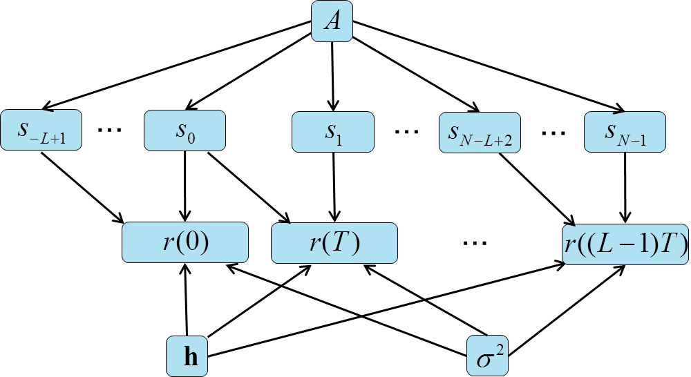
where $\mathrm{P}\mathrm{a}_{X_{k}}$ represents a subset of the variables $\left(X_{1},\cdots,X_{k-1}\right)$. By the chain rule, the factorization (9) states that, when conditioning on all the variables $\left(X_{1},\cdots,X_{k-1}\right)$, each variable $X_{k}$ is only influenced by the “parent” variables $\mathrm{P}\mathrm{a}_{X_{k}}$ (i.e., we have the Markov chain $\left(X_{1},\cdots,X_{k-1}\right)-\mathrm{P}\mathrm{a}_{X_{k}}-X_{k}$). This statistical dependence between variable $X_{k}$ and the set of parent variables $\mathrm{P}\mathrm{a}_{X_{k}}$ is encoded in the BN by introducing a directed edge between all variables $\mathrm{P}\mathrm{a}_{X_{k}}$ and $X_{k}$. As an example, the BN encoding factorization (5), (7) is shown in Fig. 1.

III-C Markov Chain Monte Carlo

MCMC methods provide a general approach for generating $M$ samples $\mathbf{x}^{\left(1\right)},\cdots,\mathbf{x}^{\left(M\right)}$ from an arbitrary target distribution $p\left(\mathbf{X}\right)$ with the aim of estimating ensemble averages, and hence multidimensional integrals such as in (8). MCMC methods simulate a Markov chain whose equilibrium distribution is $p\left(\mathbf{X}\right)$ in order to produce such samples [8]. For instance, the marginal of a joint distribution $p\left(\mathbf{X}\right)$ with respect to any variable $X_{i}$ in $\mathbf{X}$ can be estimated by MCMC as

$$p\left(X_{i}=x_{i}\right)\approx\frac{1}{M}\sum_{m=M_{0}+1}^{M_{0}+M}\mathrm{\mathbf{1}}\left(\mathbf{x}_{i}^{\left(m\right)}=x_{i}\right),$$ (10)

where $\mathbf{x}_{i}^{\left(m\right)}$ is the $i$th element of the $m$th sample of the simulated Markov chain and $x_{i}$ is a value in the domain of $X_{i}$. Note that, in (10), the first $M_{0}$ samples generated by the Markov chain are not used in order to limit the impact of the initialization.

Gibbs sampling [8] is a classical MCMC algorithm, whereby, at each step $m$, a new sample of a given random variable $X_{i}$ is generated according to the conditional distribution $p(X_{i}|\mathbf{X}_{-i}=\mathbf{x}_{-i}^{\left(m-1\right)})$, where $\mathbf{X}_{-i}$ denotes all variables in $\mathbf{X}$ except $X_{i}$, which are fixed to the current value $\mathbf{x}_{-i}^{\left(m-1\right)}$. Gibbs sampling is known to provide asymptotically correct estimates (10) (with probability one) under appropriate conditions. A sufficient condition for convergence is that the conditional distributions $p(X_{i}|\mathbf{X}_{-i})$ are strictly positive in their domains for all $i$ [8, Ch. 12]. As we will see, this condition is not satisfied by the distribution (5) for the problem under study. This suggests that more sophisticated strategies than conventional Gibbs sampling are needed, as discussed in the next section.

IV Gibbs Sampling for Modulation Classification

In this section, we design a Gibbs sampler that performs modulation classification in the presence of frequency-selective fading. As outlined in the previous section, the goal is to estimate the posterior probability $p\left(A|\mathbf{r}\right)$ in (8).

IV-A Conventional Gibbs Sampling

We first elaborate on the conventional Gibbs sampler for the calculation of the posterior $p\left(A|\mathbf{r}\right)$ that is based directly on the joint distribution (5)-(7). The corresponding BN $\mathcal{G}_{1}$ is shown in Fig. 1.

Figure 1: BN $\mathcal{G}_{1}$ for modulation classification based on the factorization (5).

As per the discussion in the previous section, Gibbs sampling requires the knowledge of the conditional distributions of each variable given all others. Calculating these conditional probabilities requires to multiply all the factors in the factorization (5)-(7) that contain the variable of interest and then normalize the resulting distribution [8, Ch. 12] . This leads to the following (see also [5]):

$$p\left(A\Big{|}\mathbf{s},\mathbf{\mathbf{\mathbf{h\mathrm{,\sigma^{2}}},\mathbf{r}}}\right)\propto p\left(A\right)\left\{\prod_{n=-L+1}^{N-1}p\left(s_{n}|A\right)\right\},$$ (11)

$$p\left(s_{n}\Big{|}A,\mathbf{s}_{-n},\mathbf{h\mathrm{,\sigma^{2},}}\mathbf{r}\right)\propto p\left(s_{n}|A\right)p\left(\mathbf{r}\Big{|}A,\mathbf{s},\mathbf{h\mathrm{,\sigma^{2}}}\right),$$ (12)

$$\mathbf{h}\Big{|}\left(A,\mathbf{s},\mathbf{h\mathrm{,\sigma^{2},}}\mathbf{r}\right)\sim\mathcal{CN}(\mathbf{h}_{*},\boldsymbol{\Sigma}_{*}),$$ (13)

$$\mathrm{and}\,\,\sigma^{2}\Big{|}\left(A,\left\{s_{n}\right\}_{n=-L+1}^{N-1},\mathbf{\mathbf{\mathbf{h\mathrm{,}}\mathbf{r}}}\right)\sim\mathcal{IG}\left(\alpha,\beta\right),$$ (14)

where $h_{*}=\boldsymbol{\Sigma}_{*}(\mathbf{\boldsymbol{\Sigma}}_{0}^{-1}\mathbf{h}_{0}+\frac{\mathbf{S}^{H}\mathbf{r}}{\sigma^{2}}),$ $\mathbf{\boldsymbol{\Sigma}}_{*}^{-1}=\mathbf{\boldsymbol{\Sigma}}_{0}^{-1}+\frac{\mathbf{S}^{H}\mathbf{S}}{\sigma^{2}},$ $\alpha=\alpha_{0}+N$ and $\beta=\beta_{0}+\left\|\mathbf{r}-\mathbf{Sh}\right\|^{2}$. Note that (13) follows from standard MMSE estimation results (see, e.g., [8]) and that (14) is a consequence of the fact that the inverse Gamma distribution is the conjugate prior for the Gaussian likelihood [9].

Gibbs sampling starts with an arbitrary feasible initialization for all variables. In particular, one needs to initialize the constellation $A$ to some value $A=a$ and, correspondingly, the transmitted symbols $\mathbf{s}$ to source values belonging to the constellation $a$. Using (11) and (12), it can be easily seen that conventional Gibbs sampling will never select values of $A$ different from the initial value $a$. This is due to the fact that the conditional distribution $p\left(s_{n}|A\right)$ gives zero probability to all values of $s_{n}$ not belonging to $A$. As a result, Gibbs sampling fails to converge to the posterior distribution (see also Sec. III). Next, we demonstrate how this problem can be solved by the proposed approach based on the latent Dirichlet BN.

IV-B Gibbs Sampling Based on Latent Dirichlet BN

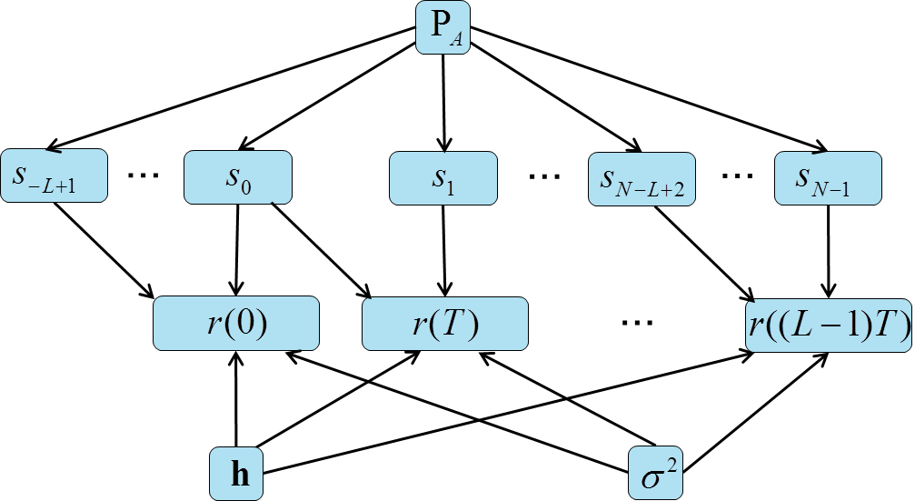
In order to avoid the problem described above, we propose to base the Gibbs sampler on the BN $\mathcal{G}_{2}$ shown in Fig. 2. In this BN, each transmitted symbol $s_{n}$ is distributed according to a random mixture of uniform distributions on the different constellations. Specifically, we introduce a random vector $\mathbf{P}_{A}$ to represent the mixture weights, so that $\mathbf{P}_{A}\left(a\right)$ is the probability that $s_{n}$ takes values in the constellation $a\mathcal{\in A}$. The prior distribution of $\mathbf{P}_{A}$ is Dirichlet, so that we have $\mathbf{P}_{A}\sim\mathrm{Dirichlet}\left(\boldsymbol{\gamma}\right)$ for a given set of nonnegative parameters $\boldsymbol{\gamma}=[\gamma_{1},\cdots,\gamma_{\left|\mathcal{A}\right|}]^{T}$ [8]. When conditioned on $\mathbf{P}_{A}$, the transmitted symbol variables $s_{n}$ are independent and distributed according to a mixture of uniform distributions, i.e., $p\left(s_{n}|\mathbf{P}_{A}\right)=\sum_{a:\,s_{n}\in a}\mathbf{P}_{A}\left(a\right)/\left|a\right|$.

The BN $\mathcal{G}_{2}$, while departing from the original model (5)-(7), has the advantage that a Gibbs sampler based on it is not limited by the zeros present in the distribution (5)-(7). In particular, thanks to the introduction of the latent variable $\mathbf{P}_{A}$, Gibbs sampling is able to explore different constellations irrespective of its initialization. The idea of introducing the latent Dirichlet variable $\mathbf{P}_{A}$ is inspired by [10], where a similar quantity was used to account for the distribution of topics within a document. According to the BN in Fig. 2, the joint pdf $p\left(\mathbf{P}_{A},\mathbf{s},\mathbf{h}\mathrm{,\sigma^{2}},\mathbf{r}\right)$ can be factorized as

$$p\left(\mathbf{P}_{A},\mathbf{s},\mathbf{h}\mathrm{,\sigma^{2}},\mathbf{r}\right)$$

$$= p\left(\mathbf{P}_{A}\right)\left\{\prod_{n=-L+1}^{N-1}p\left(s_{n}|\mathbf{P}_{A}\right)\right\}p\left(\mathbf{h}\right)\cdot$$

$$\cdot p\left(\sigma^{2}\right)p\left(\mathbf{r}\Big{|}\mathbf{s},\mathbf{h\mathrm{,\sigma^{2}}}\right),$$ (15)

where, as discussed above, we have $\mathbf{P}_{A}\sim\mathrm{Dirichlet}(\boldsymbol{\gamma})$ and $p\left(s_{n}|\mathbf{P}_{A}\right)=\sum_{a:\,s_{n}\in a}\mathbf{P}_{A}\left(a\right)/\left|a\right|$, while the remaining conditional distributions are as in (6) and (7).

Figure 2: BN $\mathcal{G}_{2}$ for the proposed modulation classification scheme based on the Dirichlet latent variable $\mathbf{P}_{A}$.

To apply Gibbs sampling based on the factorization (15), the conditional distributions for $\mathbf{P}_{A}$, $s_{n}$, $\mathbf{h}$ and $\mathrm{\sigma^{2}}$ conditioned on all other variables are required. It can be shown that the conditional distribution for $\mathbf{h}$ and $\sigma^{2}$ are (13) and (14) respectively. The other required conditional distributions of $\mathbf{P}_{A}$ and $s_{n}$ are as follows:

$$\mathbf{P}_{A}\Big{|}\left(\mathbf{s},\mathbf{h}\mathrm{,\sigma^{2}},\mathbf{r}\right)\sim\mathrm{Dirichlet}\left(\boldsymbol{\gamma}+\mathbf{c}\right),$$ (16)

where $\mathbf{c}=\left[c_{1},\cdots,c_{\left|\mathcal{A}\right|}\right]^{T}$ and $c_{a}$ is the number of symbols that belong to constellation $a\in\mathcal{A}$;

$$\mathrm{and}\,\, p\left(s_{n}\Big{|}\mathbf{P}_{A},\left\{s_{k}\right\}_{k\neq n}^{N-1},\mathbf{h\mathrm{,\sigma^{2},}}\mathbf{r}\right)$$

$$\propto p\left(s_{n}|\mathbf{P}_{A}\right)p\left(\mathbf{r}\Big{|}\mathbf{s},\mathbf{h\mathrm{,\sigma^{2}}}\right).$$ (17)

Note that (16) follows the fact that different modes of the mixture distribution is distributed as a categorical distribution and Dirichlet distribution is the conjugate prior for categorical distribution [8].

The task of modulation classification is achieved by computing the posterior distribution $p\left(\mathbf{P}_{A}|\mathbf{r}\right)$ following the Gibbs procedure discussed above. From the posterior $p\left(\mathbf{P}_{A}|\mathbf{r}\right)$, we can then obtain an estimate $\hat{A}$ for the constellation as

$$\hat{A}=\arg\max_{a\in\mathcal{A}}E\left[\mathbf{P}_{A}\left(a\right)\mid\mathbf{r}\right],$$ (18)

where the expectation is taken over the distribution $p\left(\mathbf{P}_{A}|\mathbf{r}\right)$.

Remark 1: The method proposed in [5], based on the introduction of a “superconstellation”, can be seen as an approximation of the approach presented above. Specifically, the scheme of [5] is obtained by setting $\boldsymbol{\gamma}=\mathbf{0}$ and by choosing $\mathbf{P}_{A}$ to be equal to $\mathbf{c}/\sum_{a=1}^{\left|\mathcal{A}\right|}c_{a}$, at each Gibbs iteration, where we recall that $c_{a}$ is the number of symbols that belong to constellation $a\in\mathcal{A}$. Furthermore, the computational complexity of the proposed scheme is comparable to the superconstellation Gibbs sampler [5, Table I].

Remark 2: At high signal-to-noise ratios (SNR), the relationship between $\mathbf{r}$ and $\mathbf{s}$ defined by (6) is almost deterministic. Following the discussion in the previous section, this may create convergence problems. This issue can be tackled via the idea of annealing [8, Ch. 12]. Accordingly, the distribution (6) is modified as $\mathbf{r}\Big{|}\left(A,\mathbf{s},\mathbf{h\mathrm{,\sigma^{2}}}\right)\sim\mathcal{CN}(\mathbf{Sh},\rho\sigma^{2}\mathbf{I})$, where $\rho$ is a “temperature” parameter. The procedure starts with a high value of $\rho$ to prevent the mentioned convergence problems, and then cools to a lower temperature to produce the desired target distribution. Effective cooling schedules include logarithmic and linear decreases of the temperature, whose parameters can be determined based on preliminary runs [11].

V Numerical Results and Concluding Remarks

In this section, we evaluate the performance of the proposed scheme for the recognition of three modulation formats, namely QPSK, 8-PSK and 16-QAM. We assume Rayleigh fading channels, which are normalized so that $E[\left\|\mathbf{h}\right\|^{2}]=1$. The average SNR is defined as SNR$=1/\mathrm{\sigma^{2}}$. The number of samples used by Gibbs sampling are $M=300$ and $M_{0}=100$ in (10). No annealing is used. The performance criterion of interest is probability of correct classification (PCC).

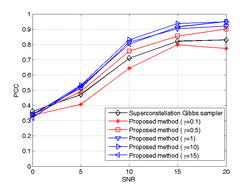
In Fig. 3, we plot the PCC for $L=3$ independent taps with relative powers given by $\left[0\mathrm{dB},-0.9\mathrm{dB},-4.9\mathrm{dB}\right]$. The performance of the proposed method is compared to the superconstellation Gibbs sampler of [5]. The prior distribution $\mathrm{Dirichlet}\left(\boldsymbol{\gamma}\right)$ for $\mathbf{P}_{A}$ is selected so that all elements of the vector $\mathbf{\mathbf{\boldsymbol{\gamma}}}$ are identical and equal to a parameter $\gamma$. In order to investigate the impact of prior distributions for $\mathbf{P}_{A}$ on the classification performance, five values, $0.1$, $0.5$, $1$, $10$ and $15$ are considered for $\gamma$. It is observed that the performance is enhanced with a larger $\gamma$, especially for higher SNR values. This is because increasing $\gamma$ enhances the relative importance of the prior distribution and helps improve the convergence properties of the algorithm (see Remark 2). We observe that in practice the value of the hyperparameter $\gamma$, as is the case for all of MCMC methods [12], can be determined based on offline preliminary runs. Finally, for sufficiently high SNRs, the superconstellation Gibbs sampler achieves a PCC of about $83\%$, while the proposed scheme achieves a PCC of $95\%$ with $\gamma=15$.

Figure 3: Probability of correct classification using the proposed method and the superconstellation Gibbs sampling of [5] versus SNR with $L=3$ independent taps.

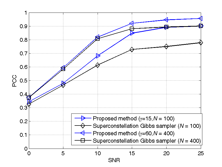
Fig. 4 shows the PCC for channels with two paths with non-integer delays $\left[0,1.3T\right]$ and with relative powers $\left[0\mathrm{dB},-0.9\mathrm{dB}\right]$ [13, Ch. 3]. A raised cosine pulse shape with roll-off factor 0.3 is assumed and we set $L=6$. For $N=100$, while there is performance degradation as compared to 3-tap channels due to more severe frequency selectivity, the proposed scheme still can achieve above $90\%$ PCC at sufficiently large SNR, while the method of [5] achieves a PCC of $80\%$. For $N=400$, both classification schemes obtain performance gains, but the proposed scheme attains a PCC of $95.6\%$, while the superconstellation method achieves a PCC of $90\%$.

Figure 4: Probability of correct classification using the proposed method and the superconstellation Gibbs sampling of [5] versus SNR with two paths and non-integer delays ($L=6$).

In summary, as demonstrated by the discussed numerical results, the proposed Gibbs sampling method based on latent Dirichlet Bayesian network provides significant performance gains over the state of the art.

References

- [1] O. A. Dobre, A. Abdi, Y. Bar-Ness and W. Su, “A survey of automatic modulation classification techniques: classical approaches and new developments,” IET Communications, vol.1, no. 2, pp. 137-156, Apr. 2007.
- [2] N. Lay and A. Polydoros, “Modulation classification of signals in unknown ISI environments,” in Proc. IEEE MILCOM, pp. 170-174, San Diego, CA, Nov. 1995.
- [3] P. Panagiotou, A. Anastasopoulos, and A. Polydoros, “Likelihood ratio tests for modulation classification," in Proc. IEEE MILCOM, pp. 670-674, Los Angeles, CA, Oct. 2000,
- [4] F. Hameed, O. A. Dobre, and D. C. Popescu, “On the likelihood-based approach to modulation classification," IEEE Trans. Wireless Commun., vol. 8, no. 12, pp. 5884-5892, Dec. 2009.
- [5] T. A. Drumright and Z. Ding. “QAM constellation classication based on statistical sampling for linear distortive channels,” IEEE Trans. Signal Process., vol. 54, no. 5, pp. 1575-1586, May 2006.
- [6] A. Doucet and X. Wang, “Monte Carlo methods for signal processing,” IEEE Signal Process. Mag., vol. 22, no. 6, pp. 152–170, Nov. 2005.
- [7] J. R. Barry, E. A. Lee and D. G. Messerschmitt, Digital Communication, Springer, 2003.
- [8] D. Koller and N. Friedman, Probabilistic Graphical Models: Principles and Techniques, MIT Press, 2009.
- [9] K. P. Murphy, “Conjugate Bayesian analysis of the Gaussian distribution,” Univ. of British Columbia, Canada, Tech. Rep., 2007 [Online]. Available: http://www.cs.ubc.ca/~murphyk/Papers/bayesGauss.pdf
- [10] D. Blei, A. Ng, and M. Jordan. “Latent Dirichlet allocation,” Journal of Machine Learning Research, vol. 3, pp. 993–1022, Jan. 2003.
- [11] Y. Nourani and B. Andresen, “A comparison of simulated annealing cooling strategies,” J. Phys. A, vol. 31, no. 41, pp. 8373-8385, July 1998.
- [12] R. M. Neal, “Sampling from multimodal distributions using tempered transitions,” Statistics and computing, vol. 6, no. 4, pp. 353-366, June 1996.
- [13] A. Goldsmith, Wireless Communications, Cambridge University Press, 2005.