ULB-TH/14-12

Lepton Flavor Violation in Flavored Gauge Mediation

Lorenzo Calibbia, Paride Paradisib,c,d, Robert Zieglere,f

aService de Physique Théorique, Université Libre de Bruxelles, B-1050 Brussels, Belgium
bDipartimento di Fisica e Astronomia, Universitá di Padova, Via Marzolo 8, I-35131 Padova, Italy
cINFN Sezione di Padova, Via Marzolo 8, I-35131 Padova, Italy
dSISSA, Via Bonomea 265, I-34136 Trieste, Italy
eSorbonne Universités, UPMC Univ Paris 06, UMR 7589, LPTHE, F-75005, Paris, France
fCNRS, UMR 7589, LPTHE, F-75005, Paris, France

We study the anatomy and phenomenology of Lepton Flavor Violation (LFV) in the context of Flavored Gauge Mediation (FGM). Within FGM, the messenger sector couples directly to the MSSM matter fields with couplings controlled by the same dynamics that explains the hierarchies in the SM Yukawas. Although the pattern of flavor violation depends on the particular underlying flavor model, FGM provides a built-in flavor suppression similar to wave function renormalization or SUSY Partial Compositeness. Moreover, in contrast to these models, there is an additional suppression of left-right (LR) flavor transitions by third-generation Yukawas that in particular provides an extra protection against flavor-blind phases. We exploit the consequences of this setup for lepton flavor phenomenology, assuming that the new couplings are controlled by simple U(1)𝑈1U(1) flavor models that have been proposed to accommodate large neutrino mixing angles. Remarkably, it turns out that in the context of FGM these models can pass the impressive constraints from LFV processes and leptonic EDMs even for light superpartners, therefore offering the possibility of resolving the longstanding muon g2𝑔2g-2 anomaly.

1 Introduction

One of the longstanding problems in particle physics is the origin of flavor hierarchies in the Standard Model (SM). The most popular attempt to address this problem is in terms of flavor symmetries in which the flavor hierarchies arise from a suitable symmetry breaking pattern. Among the numerous possibilities, the simplest models are based on a single U(1)𝑈1U(1) flavor symmetry [1, 2, 3, 4]. In the quark sector this ansatz works pretty well and can account for all hierarchies in quark masses and mixing, with an order-of-magnitude prediction VubVusVcbsimilar-tosubscript𝑉𝑢𝑏subscript𝑉𝑢𝑠subscript𝑉𝑐𝑏V_{ub}\sim V_{us}V_{cb} that is in good agreement with data. Also in the lepton sector a single U(1)𝑈1U(1) works very well, since charge lepton mass hierarchies can arise from large charge differences of right-handed leptons, while large mixing angles are due to small charge differences of left-handed leptons. In this way U(1)𝑈1U(1) models can naturally realize the paradigm of an “anarchical” structure [5, 6, 7, 8] in lepton mixing, which has recently received renewed attention [9, 10, 11] after the reactor neutrino angle θ13subscript𝜃13\theta_{13} turned out to be sizable.

Independently of the nature of the underlying flavor symmetry, the crucial question about these kind of models regard their predictivity. Since flavor models aim at explaining the origin of dimensionless Yukawa couplings, there is no preferred mass scale of the new degrees of freedom. As new effects in the SM flavor sector are suppressed by this mass scale, there are no observable deviations from the SM flavor predictions, unless this scale is unexpectedly light [12]. Therefore the only way to test these models in laboratory experiments for a high-scale flavor sector is the presence of new physics around the TeV scale, as suggested by the hierarchy problem. If such physics comes with a flavor structure, it can possibly carry down the information of the high-scale flavor sector to the TeV scale and lead to testable predictions for precision flavor observables. The prime example is Supersymmetry (SUSY), which in the case of high-scale mediation of SUSY breaking around or above the flavor sector scale directly contains the imprint of the flavor symmetry in the soft-breaking sfermion masses.

However, within the context of Gravity Mediation simple U(1)𝑈1U(1) models are in big trouble as the suppression of flavor violation is too weak. The reason is that off-diagonal entries in the left-handed and right-handed sfermion mass matrices are suppressed by the differences of the corresponding charges due to their non-holomorphic nature. In the left-handed sector these charge differences are directly related to mixing angles, which for the first two generations are sizable both in the lepton and quark sector. Since the strongest constraint precisely arise from observables involving light families, like ϵKsubscriptitalic-ϵ𝐾\epsilon_{K} and μeγ𝜇𝑒𝛾\mu\to e\gamma, such U(1)𝑈1U(1) flavor models in the context of Gravity Mediation are essentially incompatible with SUSY around the TeV scale.111This conclusion holds even under the assumption of a mechanism inducing degenerate sfermion masses at the SUSY breaking mediation scale. In fact, the assumed flavor universality is broken by the renormalization group evolution of the soft masses down to the flavor breaking scale, so that large flavor mixing is anyway generated at the level predicted by the U(1)𝑈1U(1) symmetry [13].

The situation is completely different in Gauge Mediation (see Ref. [14]), where the SUSY breaking and the flavor sector can be decoupled. Indeed, if the flavor scale is much higher than the SUSY messenger scale then soft masses are screened from the high-energy flavor sector and have a flavor structure determined only by SM Yukawas, thus realizing the paradigm of Minimal Flavor Violation (MFV) [15]. While this scenario provides a very appealing mechanism to solve the SUSY flavor problem, the imprint of the flavor sector in low-energy physics and thus the possibility to test flavor symmetry models is completely lost.

It is therefore interesting to construct extensions of Minimal Gauge Mediation (MGM) that re-introduce the dependence on the underlying flavor sector, and thus lead to a broad variety of sfermion flavor structures beyond MFV. An example for such extensions is provided by a class of models that has been dubbed “Flavored Gauge Mediation” (FGM) [16]. In these scenarios, new direct couplings between the messengers and the MSSM matter fields are introduced with a flavor structure that is assumed to be controlled by the same underlying flavor symmetry that explains the smallness of the Yukawas.222Such matter-messenger couplings have recently received new interest, as they allow to obtain a large Higgs mass with light stops by generating non-vanishing A-terms at the messenger scale [17, 18, 19, 20, 21, 22, 23, 24, 25, 26, 27]. These couplings generate new contributions to sfermion masses (on top of of the flavor-universal MGM ones) that are controlled by the underlying flavor symmetry. Interestingly, due to the loop origin of the soft terms, there is a built-in suppression of flavor violation that is independent of the underlying flavor model [28]. This implies that even single U(1)𝑈1U(1) flavor models are perfectly viable (in contrast to Gravity Mediation), as the flavor pattern of the resulting sfermion masses resembles the suppression in wave function renormalization [29, 30] or SUSY Partial Compositeness [31, 32]. Moreover, in contrast to those scenarios, there is also a built-in suppression of LR flavor transitions and in particular flavor-blind phases by third-generation Yukawas, which becomes very efficient in the down and charged-lepton sector provided tanβ𝛽\tan\beta is not very large.

While in Ref. [28] we have focused on the quark sector, in this paper we analyze the impact of FGM models with underlying U(1)𝑈1U(1) flavor models on the lepton sector. There are good arguments that motivate this study: i) in contrast to the quark sector the large neutrino mixing angles require milder hierarchies in left-handed charges, leading in turn to weaker suppression in the left-handed slepton sector and therefore potentially large effects in LFV processes, ii) the experimental bounds on LFV channels with an underlying μe𝜇𝑒\mu\to e transition as well as the electron EDM underwent recently a very significant improvement challenging many models with New Physics (NP) at the TeV scale, even with modest sources of flavor violation. Therefore the major aim of this work is to analyze whether and to which extent single U(1)𝑈1U(1) flavor models for the lepton sector are viable in the context of FGM. A related question is whether we can account for the current muon g2𝑔2g-2 anomaly, that is if light sleptons are still allowed by the LFV and EDM bounds (for a general discussion on the interrelationship of leptonic dipoles see Ref. [33]).

The rest of the paper is organized as follows: in Section 2 we recall the main ingredients of FGM models providing explicit expressions for the soft masses in the slepton sector. Concrete examples of U(1)𝑈1U(1) leptonic flavor models and their imprint in the soft sector are presented in Section 3. The low-energy phenomenology of FGM models supplemented by the above U(1)𝑈1U(1) flavor models is studied in Section 4. In Section 5, we compare the flavor structure of the soft terms and related phenomenological implications of FGM models to U(1)𝑈1U(1) models with Gravity Mediation and models with SUSY Partial Compositeness. We conclude in Section 6. In an appendix we collect the formulae for LFV branching ratios, lepton anomalous magnetic moments and lepton electric dipole moments using a generalized mass insertion approximation without assuming large tanβ𝛽\tan\beta, thus improving on existing results that take into account only the tanβ𝛽\tan\beta enhanced terms.

2 Flavored Gauge Mediation

We begin with a brief review of Minimal Gauge Mediation (see Ref. [14]). In this scenario N𝑁N copies of heavy chiral superfields Φi+Φ¯isubscriptΦ𝑖subscript¯Φ𝑖\Phi_{i}+\overline{\Phi}_{i} in 𝟓+𝟓¯5¯5{\bf 5+\overline{5}} of SU(5) are introduced. These messenger fields couple directly to the SUSY breaking sector, which is effectively parameterized by a single spurion field X𝑋X that gets a vev X=M+Fθ2delimited-⟨⟩𝑋𝑀𝐹superscript𝜃2\langle X\rangle=M+F\theta^{2}. Through the following superpotential coupling

WXΦ¯iΦi,i=1N,formulae-sequence𝑋subscript¯Φ𝑖subscriptΦ𝑖𝑊𝑖1𝑁W\supset X\overline{\Phi}_{i}\Phi_{i},\qquad i=1\ldots N\,, (1)

the messengers acquire large supersymmetric mass terms M𝑀M and SUSY breaking masses proportional to F𝐹F. By integrating out the messengers at loop-level, soft terms are generated. At the messenger scale, A-terms vanish and gaugino masses and sfermion masses are given by

Mi(M)=Nαi(M)4πΛ,Λ=FM,formulae-sequencesubscript𝑀𝑖𝑀𝑁subscript𝛼𝑖𝑀4𝜋ΛΛ𝐹𝑀\displaystyle M_{i}(M)=N\frac{\alpha_{i}(M)}{4\pi}~{}\Lambda,\qquad\qquad\Lambda=\frac{F}{M}, (2)
mf~2(M)=2Ni=13Ci(f)αi2(M)(4π)2Λ2,f=q,u,d,,formulae-sequencesubscriptsuperscript𝑚2~𝑓𝑀2𝑁superscriptsubscript𝑖13subscript𝐶𝑖𝑓subscriptsuperscript𝛼2𝑖𝑀superscript4𝜋2superscriptΛ2𝑓𝑞𝑢𝑑\displaystyle m^{2}_{\tilde{f}}(M)=2N\sum_{i=1}^{3}C_{i}(f)~{}\frac{\alpha^{2}_{i}(M)}{(4\pi)^{2}}~{}\Lambda^{2},\qquad f=q,\,u,\,d,\ldots, (3)

where Ci(f)subscript𝐶𝑖𝑓C_{i}(f), i=1,2,3𝑖123i=1,2,3 is the quadratic Casimir of the representation of the field f𝑓f under the gauge group SU(3)×SU(2)×U(1)SU3SU2U1{\rm SU(3)}\times{\rm SU(2)}\times{\rm U(1)}.

Since the messengers have the same gauge quantum numbers as the MSSM Higgs fields, in addition to the Yukawa couplings

W(yU)ijQiUjHu+(yD)ijQiDjHd+(yE)ijLiEjHd,subscriptsubscript𝑦𝑈𝑖𝑗subscript𝑄𝑖subscript𝑈𝑗subscript𝐻𝑢subscriptsubscript𝑦𝐷𝑖𝑗subscript𝑄𝑖subscript𝐷𝑗subscript𝐻𝑑subscriptsubscript𝑦𝐸𝑖𝑗subscript𝐿𝑖subscript𝐸𝑗subscript𝐻𝑑𝑊W\supset(y_{U})_{ij}Q_{i}U_{j}H_{u}+(y_{D})_{ij}Q_{i}D_{j}H_{d}+(y_{E})_{ij}L_{i}E_{j}H_{d}\,, (4)

also direct couplings of messengers to MSSM fields are allowed by the gauge symmetries. If we restrict to R-parity even messenger fields,333For R-parity odd messengers similar couplings to Higgs fields are allowed and have been discussed in the literature, see e.g. [25]. Note that in this way one preserves the MFV structure of MGM. Here we are instead interested in non-trivial flavor structures. the messengers can couple only to the MSSM matter fields. For the messenger doublets these couplings read in general

ΔWΔ𝑊\displaystyle\Delta W =(λU)ijQiUjΦHu+(λD)ijQiDjΦ¯Hd+(λE)ijLiEjΦ¯Hd,absentsubscriptsubscript𝜆𝑈𝑖𝑗subscript𝑄𝑖subscript𝑈𝑗subscriptΦsubscript𝐻𝑢subscriptsubscript𝜆𝐷𝑖𝑗subscript𝑄𝑖subscript𝐷𝑗subscript¯Φsubscript𝐻𝑑subscriptsubscript𝜆𝐸𝑖𝑗subscript𝐿𝑖subscript𝐸𝑗subscript¯Φsubscript𝐻𝑑\displaystyle=(\lambda_{U})_{ij}Q_{i}U_{j}\Phi_{H_{u}}+(\lambda_{D})_{ij}Q_{i}D_{j}\overline{\Phi}_{H_{d}}+(\lambda_{E})_{ij}L_{i}E_{j}\overline{\Phi}_{H_{d}}, (5)

where ΦHu,Φ¯HdsubscriptΦsubscript𝐻𝑢subscript¯Φsubscript𝐻𝑑\Phi_{H_{u}},\overline{\Phi}_{H_{d}} denote the SU(2) doublet components of the 𝟓,𝟓¯5¯5\bf 5,\bf\overline{5} messengers, and we restricted to the case of one messenger pair for simplicity.

The presence of direct messenger-matter couplings gives rise to new contributions to sfermion masses and A-terms with a flavor structure that depends on the new parameters λijsubscript𝜆𝑖𝑗\lambda_{ij}. If these couplings were flavor-anarchic 𝒪(1)𝒪1\mathcal{O}\left(1\right) numbers, the elegant solution of Gauge Mediation to the SUSY flavor problem would be completely spoiled. Therefore it is usually assumed that all direct couplings of the messengers to matter fields vanish, which can be enforced for example by introducing a new Z2subscript𝑍2Z_{2} symmetry under which MSSM fields are even and messengers are odd. Note that this symmetry extends to a full accidental U(1)𝑈1U(1) symmetry in the case of one messenger pair

ΦΦ\displaystyle\Phi eiαΦ,absentsuperscript𝑒𝑖𝛼Φ\displaystyle\to e^{i\alpha}\Phi, Φ¯¯Φ\displaystyle\overline{\Phi} eiαΦ¯.absentsuperscript𝑒𝑖𝛼¯Φ\displaystyle\to e^{-i\alpha}\overline{\Phi}. (6)

However, in order to preserve the neat solution of the SUSY flavor problem in MGM, it is enough that the new couplings in Eq. (5) are just sufficiently small. Such small couplings can be easily motivated in the context of flavor models, since they break the global flavor symmetries of MSSM kinetic terms exactly as the Yukawas, and therefore they can naturally have a similar hierarchical structure. This can be realized in explicit flavor models in which the messenger fields transform like the Higgs fields (in particular one can choose that they do not transform at all under the flavor sector), which implies that the new couplings have the same parametric suppression as the Yukawas,

λUsubscript𝜆𝑈\displaystyle\lambda_{U} yU,similar-toabsentsubscript𝑦𝑈\displaystyle\sim y_{U}, λDsubscript𝜆𝐷\displaystyle\lambda_{D} yD,similar-toabsentsubscript𝑦𝐷\displaystyle\sim y_{D}, λEsubscript𝜆𝐸\displaystyle\lambda_{E} yE.similar-toabsentsubscript𝑦𝐸\displaystyle\sim y_{E}. (7)

Following Ref. [16], we refer to these kind of models as “Flavored Gauge Mediation” (FGM).

The new contributions to soft terms induced by the couplings in Eq. (5) can be calculated using the general expressions in Ref. [25]. At leading order in SUSY breaking one finds new contributions to sfermion masses at 2-loop and non-vanishing A-terms at 1-loop. While these new effects can have interesting consequences for the low-energy spectrum [34, 35], here we are mainly interested in the flavor structure of the new contributions to sfermion masses, in particular in the slepton sector. Therefore we will now take a bottom-up point of view and restrict the analysis to the consequences of the presence of the λEsubscript𝜆𝐸\lambda_{E} coupling for the lepton sector. We will not discuss the impact of other possible messenger-matter couplings on the low-energy spectrum, in particular the mass of the lightest Higgs boson. We just note that the Higgs mass does not represent a serious constraint in these kind of models, and can be due to large A-terms or an implementation in the NMSSM. The latter also represents a natural possibility to generate the μlimit-from𝜇\mu-term and to elegantly solve the μBμ𝜇subscript𝐵𝜇\mu-B_{\mu} problem of Gauge Mediation, since in the NMSSM the general structure of FGM motivates a direct coupling of the NMSSM singlet to the messengers which can easily allow for correct EWSB [21, 36].

Furthermore, let us notice that the couplings λEsubscript𝜆𝐸\lambda_{E} do not deform the spectrum predicted by the underlying gauge mediation scheme, at least for low to moderate values of tanβ𝛽\tan\beta, as we are going to consider in the next sections. In particular, if mh126subscript𝑚126m_{h}\approx 126 GeV is accounted for by a large top A-term, induced by an 𝒪(1)𝒪1\mathcal{O}(1) coupling (λU)33subscriptsubscript𝜆𝑈33(\lambda_{U})_{33} in Eq. (5), the spectrum would resemble the one discussed e.g. in Ref. [28]. This would have interesting consequences for the leptonic sector we consider here, since (λU)33=𝒪(1)subscriptsubscript𝜆𝑈33𝒪1(\lambda_{U})_{33}=\mathcal{O}(1) also suppresses the masses of the left-handed sleptons, through an induced Fayet-Iliopoulos term, thus naturally accomodating the Higgs mass with a light slepton spectrum that can give a sizable contribution to the muon g2𝑔2g-2 [19, 28].

For soft terms in the slepton sector we use the conventions

\displaystyle{\cal L} ((m~L2)ijLiLj+(m~E2)ijEiEj+(Ae)ijLiEjHd)|scalarevaluated-atsubscriptsubscriptsuperscript~𝑚2𝐿𝑖𝑗subscript𝐿𝑖superscriptsubscript𝐿𝑗subscriptsubscriptsuperscript~𝑚2𝐸𝑖𝑗superscriptsubscript𝐸𝑖subscript𝐸𝑗subscriptsubscript𝐴𝑒𝑖𝑗subscript𝐿𝑖subscript𝐸𝑗subscript𝐻𝑑𝑠𝑐𝑎𝑙𝑎𝑟absent\displaystyle\supset-\left((\tilde{m}^{2}_{L})_{ij}L_{i}L_{j}^{\dagger}+(\tilde{m}^{2}_{E})_{ij}E_{i}^{\dagger}E_{j}+(A_{e})_{ij}L_{i}E_{j}H_{d}\right)|_{scalar}
=(l~LTm~L2l~L+e~RT(m~E2)ije~R+l~LTAee~RHd),absentsuperscriptsubscript~𝑙𝐿𝑇subscriptsuperscript~𝑚2𝐿superscriptsubscript~𝑙𝐿superscriptsubscript~𝑒𝑅𝑇subscriptsubscriptsuperscript~𝑚2𝐸𝑖𝑗superscriptsubscript~𝑒𝑅superscriptsubscript~𝑙𝐿𝑇subscript𝐴𝑒superscriptsubscript~𝑒𝑅subscript𝐻𝑑\displaystyle=-\left(\tilde{l}_{L}^{T}\tilde{m}^{2}_{L}\tilde{l}_{L}^{*}+\tilde{e}_{R}^{T}(\tilde{m}^{2}_{E})_{ij}\tilde{e}_{R}^{*}+\tilde{l}_{L}^{T}A_{e}\tilde{e}_{R}^{*}H_{d}\right), (8)

where the first line denotes the scalar components of superfields. Using the results of Ref. [25], the presence of λEsubscript𝜆𝐸\lambda_{E} gives rise to the following expressions for the non-holomorphic masses444We only consider terms in leading order in Λ2/M2superscriptΛ2superscript𝑀2\Lambda^{2}/M^{2}, i.e. a messenger scale that is not particularly low.

m~L2subscriptsuperscript~𝑚2𝐿\displaystyle{\tilde{m}}^{2}_{L} =\displaystyle= Λ2256π4[N(32g24+310g14)(95g12+3g22)λEλE\displaystyle\frac{\Lambda^{2}}{256\pi^{4}}\bigg{[}N\left(\frac{3}{2}g_{2}^{4}+\frac{3}{10}g_{1}^{4}\right)-\left(\frac{9}{5}g_{1}^{2}+3g_{2}^{2}\right)\lambda_{E}\lambda_{E}^{\dagger} (9)
+\displaystyle+ 3λEλEλEλE+2λEyEyEλE2yEλEλEyE3subscript𝜆𝐸superscriptsubscript𝜆𝐸subscript𝜆𝐸superscriptsubscript𝜆𝐸2subscript𝜆𝐸superscriptsubscript𝑦𝐸subscript𝑦𝐸superscriptsubscript𝜆𝐸2subscript𝑦𝐸superscriptsubscript𝜆𝐸subscript𝜆𝐸superscriptsubscript𝑦𝐸\displaystyle 3\lambda_{E}\lambda_{E}^{\dagger}\lambda_{E}\lambda_{E}^{\dagger}+2\lambda_{E}y_{E}^{\dagger}y_{E}\lambda_{E}^{\dagger}-2y_{E}\lambda_{E}^{\dagger}\lambda_{E}y_{E}^{\dagger}
+\displaystyle+ λEλETr(λEλE)+yEλETr(λEyE)+λEyETr(yEλE)],\displaystyle\lambda_{E}\lambda_{E}^{\dagger}{\rm Tr}\left(\lambda_{E}\lambda_{E}^{\dagger}\right)+y_{E}\lambda_{E}^{\dagger}{\rm Tr}\left(\lambda_{E}y_{E}^{\dagger}\right)+\lambda_{E}y_{E}^{\dagger}{\rm Tr}\left(y_{E}\lambda_{E}^{\dagger}\right)\bigg{]}\,,

and

m~E2subscriptsuperscript~𝑚2𝐸\displaystyle{\tilde{m}}^{2}_{E} =\displaystyle= Λ2256π4[65g14N(185g12+6g22)λEλE+6λEλEλEλE\displaystyle\frac{\Lambda^{2}}{256\pi^{4}}\bigg{[}\frac{6}{5}g_{1}^{4}N-\left(\frac{18}{5}g_{1}^{2}+6g_{2}^{2}\right)\lambda_{E}^{\dagger}\lambda_{E}+6\lambda_{E}^{\dagger}\lambda_{E}\lambda_{E}^{\dagger}\lambda_{E} (10)
+\displaystyle+ 2λEyEyEλE2yEλEλEyE+2λEλETr(λEλE)2superscriptsubscript𝜆𝐸subscript𝑦𝐸superscriptsubscript𝑦𝐸subscript𝜆𝐸2superscriptsubscript𝑦𝐸subscript𝜆𝐸superscriptsubscript𝜆𝐸subscript𝑦𝐸2superscriptsubscript𝜆𝐸subscript𝜆𝐸Trsubscript𝜆𝐸superscriptsubscript𝜆𝐸\displaystyle 2\lambda_{E}^{\dagger}y_{E}y_{E}^{\dagger}\lambda_{E}-2y_{E}^{\dagger}\lambda_{E}\lambda_{E}^{\dagger}y_{E}+2\lambda_{E}^{\dagger}\lambda_{E}{\rm Tr}\left(\lambda_{E}\lambda_{E}^{\dagger}\right)
+\displaystyle+ 2λEyETr(λEyE)+2yEλETr(yEλE)],\displaystyle 2\lambda_{E}^{\dagger}y_{E}{\rm Tr}\left(\lambda_{E}y_{E}^{\dagger}\right)+2y_{E}^{\dagger}\lambda_{E}{\rm Tr}\left(y_{E}\lambda_{E}^{\dagger}\right)\bigg{]}\,,

while the A-terms are given by

AE=Λ16π2(λEλEyE+2yEλEλE).subscript𝐴𝐸Λ16superscript𝜋2subscript𝜆𝐸superscriptsubscript𝜆𝐸subscript𝑦𝐸2subscript𝑦𝐸superscriptsubscript𝜆𝐸subscript𝜆𝐸\displaystyle A_{E}=-\frac{\Lambda}{16\pi^{2}}\left(\lambda_{E}\lambda_{E}^{\dagger}y_{E}+2y_{E}\lambda_{E}^{\dagger}\lambda_{E}\right)\,. (11)

Note that the flavor dependence of the above expressions can be obtained using a simple spurion analysis, taking into account also the U(1)M𝑈subscript1𝑀U(1)_{M} “messenger number” in Eq. (6) as a spurious symmetry under which the new couplings are charged. The U(1)M𝑈subscript1𝑀U(1)_{M} symmetry prevents terms like λEyEsubscript𝜆𝐸superscriptsubscript𝑦𝐸\lambda_{E}y_{E}^{\dagger} and λEyEsuperscriptsubscript𝜆𝐸subscript𝑦𝐸\lambda_{E}^{\dagger}y_{E} for the non-holomorphic masses m~L2subscriptsuperscript~𝑚2𝐿{\tilde{m}}^{2}_{L} and m~E2subscriptsuperscript~𝑚2𝐸{\tilde{m}}^{2}_{E}, respectively, and terms like λEsubscript𝜆𝐸\lambda_{E}, λEyEλEsubscript𝜆𝐸superscriptsubscript𝑦𝐸subscript𝜆𝐸\lambda_{E}y_{E}^{\dagger}\lambda_{E} and λEyEλEsuperscriptsubscript𝜆𝐸subscript𝑦𝐸superscriptsubscript𝜆𝐸\lambda_{E}^{\dagger}y_{E}\lambda_{E}^{\dagger} for the A-terms. As a result, the A-terms are partially aligned to the Yukawa couplings and their diagonal components are necessarily real and therefore do not induce contributions to the EDMs.

For future convenience, we define the flavor violating mass insertions (MIs) as usual

(δLLe)ijsubscriptsuperscriptsubscript𝛿𝐿𝐿𝑒𝑖𝑗\displaystyle(\delta_{LL}^{e})_{ij} =(m~L2)ijm~L2,absentsubscriptsubscriptsuperscript~𝑚2𝐿𝑖𝑗subscriptsuperscript~𝑚2𝐿\displaystyle=\frac{({\tilde{m}}^{2}_{L})_{ij}}{{\tilde{m}}^{2}_{L}}~{}, (δRRe)ijsubscriptsuperscriptsubscript𝛿𝑅𝑅𝑒𝑖𝑗\displaystyle(\delta_{RR}^{e})_{ij} =(m~E2)ijm~E2,absentsubscriptsubscriptsuperscript~𝑚2𝐸𝑖𝑗subscriptsuperscript~𝑚2𝐸\displaystyle=\frac{({\tilde{m}}^{2}_{E})_{ij}}{{\tilde{m}}^{2}_{E}}~{}, (δLRe)ijsubscriptsuperscriptsubscript𝛿𝐿𝑅𝑒𝑖𝑗\displaystyle(\delta_{LR}^{e})_{ij} =vd(AE)ijm~Lm~E.absentsubscript𝑣𝑑subscriptsubscript𝐴𝐸𝑖𝑗subscript~𝑚𝐿subscript~𝑚𝐸\displaystyle=\frac{v_{d}(A_{E})_{ij}}{{\tilde{m}}_{L}{\tilde{m}}_{E}}~{}. (12)

In the limit of yE,λE1much-less-thansubscript𝑦𝐸subscript𝜆𝐸1y_{E},\lambda_{E}\ll 1, i.e. for moderate/low tanβ𝛽\tan\beta values, we obtain the following approximate expressions at the messenger scale:

(δLLe)ijsubscriptsuperscriptsubscript𝛿𝐿𝐿𝑒𝑖𝑗\displaystyle(\delta_{LL}^{e})_{ij} (10g22+6g125g24+g14)(λEλE)ijN,similar-to-or-equalsabsent10superscriptsubscript𝑔226superscriptsubscript𝑔125superscriptsubscript𝑔24superscriptsubscript𝑔14subscriptsubscript𝜆𝐸superscriptsubscript𝜆𝐸𝑖𝑗𝑁\displaystyle\simeq-\left(\frac{10g_{2}^{2}+6g_{1}^{2}}{5g_{2}^{4}+g_{1}^{4}}\right)\frac{(\lambda_{E}\lambda_{E}^{\dagger})_{ij}}{N}\,, (δRRe)ijsubscriptsuperscriptsubscript𝛿𝑅𝑅𝑒𝑖𝑗\displaystyle(\delta_{RR}^{e})_{ij} (5g22+3g12g14)(λEλE)ijN,similar-to-or-equalsabsent5superscriptsubscript𝑔223superscriptsubscript𝑔12superscriptsubscript𝑔14subscriptsuperscriptsubscript𝜆𝐸subscript𝜆𝐸𝑖𝑗𝑁\displaystyle\simeq-\left(\frac{5g_{2}^{2}+3g_{1}^{2}}{g_{1}^{4}}\right)\frac{(\lambda_{E}^{\dagger}\lambda_{E})_{ij}}{N}\,, (13)
(δLRe)ij13N5g1g2mje(λEλE)ij+2mie(λEλE)ijm~Lm~E.similar-to-or-equalssubscriptsuperscriptsubscript𝛿𝐿𝑅𝑒𝑖𝑗13𝑁5subscript𝑔1subscript𝑔2subscriptsuperscript𝑚𝑒𝑗subscriptsubscript𝜆𝐸superscriptsubscript𝜆𝐸𝑖𝑗2subscriptsuperscript𝑚𝑒𝑖subscriptsuperscriptsubscript𝜆𝐸subscript𝜆𝐸𝑖𝑗subscript~𝑚𝐿subscript~𝑚𝐸\displaystyle(\delta_{LR}^{e})_{ij}\simeq-\frac{1}{\sqrt{\frac{3N}{\sqrt{5}}}g_{1}g_{2}}~{}\frac{m^{e}_{j}(\lambda_{E}\lambda_{E}^{\dagger})_{ij}+2m^{e}_{i}(\lambda_{E}^{\dagger}\lambda_{E})_{ij}}{\sqrt{\tilde{m}_{L}\tilde{m}_{E}}}\,. (14)

Few comments are in order:

  • The above MIs, as well as all superpotential couplings, are defined in the basis where we define the flavor model. In order to study their phenomenological consequences, we go to the mass basis for the charged lepton Yukawas by means of the rotation yEVELTyEVER=yEdiagsubscript𝑦𝐸superscriptsubscript𝑉𝐸𝐿𝑇subscript𝑦𝐸subscript𝑉𝐸𝑅superscriptsubscript𝑦𝐸𝑑𝑖𝑎𝑔y_{E}\to V_{EL}^{T}y_{E}V_{ER}=y_{E}^{diag}. Under this change of basis, the spurion λEsubscript𝜆𝐸\lambda_{E} transforms accordingly. However, one can easily check that in U(1)𝑈1U(1) models with non-negative charges the parametric flavor suppression remains the same and only the 𝒪(1)𝒪1{\cal O}(1) coefficients change. We therefore simply ignore these differences, that is we take VELTλEVERλEsimilar-tosuperscriptsubscript𝑉𝐸𝐿𝑇subscript𝜆𝐸subscript𝑉𝐸𝑅subscript𝜆𝐸V_{EL}^{T}\lambda_{E}V_{ER}\sim\lambda_{E}.

  • Interestingly, the diagonal A-terms are real. As a result, the leading CP violating phases generating the EDMs can only arise at higher order in the MIs, through the combination (δLLe)ik(δLRe)kjsubscriptsuperscriptsubscript𝛿𝐿𝐿𝑒𝑖𝑘subscriptsuperscriptsubscript𝛿𝐿𝑅𝑒𝑘𝑗(\delta_{LL}^{e})_{ik}(\delta_{LR}^{e})_{kj}, (δLRe)ik(δRRe)kjsubscriptsuperscriptsubscript𝛿𝐿𝑅𝑒𝑖𝑘subscriptsuperscriptsubscript𝛿𝑅𝑅𝑒𝑘𝑗(\delta_{LR}^{e})_{ik}(\delta_{RR}^{e})_{kj}, and (δLLe)ik(δLRe)kk(δRRe)kjsubscriptsuperscriptsubscript𝛿𝐿𝐿𝑒𝑖𝑘subscriptsuperscriptsubscript𝛿𝐿𝑅𝑒𝑘𝑘subscriptsuperscriptsubscript𝛿𝑅𝑅𝑒𝑘𝑗(\delta_{LL}^{e})_{ik}(\delta_{LR}^{e})_{kk}(\delta_{RR}^{e})_{kj} when ij=11𝑖𝑗11ij=11. This however leads to an additional suppression by powers of (λE)33yτsimilar-tosubscriptsubscript𝜆𝐸33subscript𝑦𝜏(\lambda_{E})_{33}\sim y_{\tau}.555Notice that the μ𝜇\mu- and Bμsubscript𝐵𝜇B_{\mu}-terms, which are not controlled by GMSB, could still introduce CP violating phases depending on the underlying mechanism that generates them. However, if this mechanism is such that the phases of μ𝜇\mu and Bμsubscript𝐵𝜇B_{\mu} are correlated to the phase of ΛΛ\Lambda, then no phases arise from this sector [14].

  • As a consequence of Eqs. (13),(14), the naive expectations for the MIs are enhanced, for a given number of messengers N𝑁N, by large (mediation scale dependent) gauge factors. This is especially true in the case of (δRRe)ijsubscriptsuperscriptsubscript𝛿𝑅𝑅𝑒𝑖𝑗(\delta_{RR}^{e})_{ij} and, to less extent, also in the cases of (δLLe)ijsubscriptsuperscriptsubscript𝛿𝐿𝐿𝑒𝑖𝑗(\delta_{LL}^{e})_{ij} and (δLRe)ijsubscriptsuperscriptsubscript𝛿𝐿𝑅𝑒𝑖𝑗(\delta_{LR}^{e})_{ij}.

In the following, we will analyze the impact of our FGM model on the branching ratio of μeγ𝜇𝑒𝛾\mu\to e\gamma and the electron EDM which are the most powerful probes of new physics in the leptonic sector. To do so, we need to specify the underlying flavor model that controls the flavor structure of the new couplings.

3 Flavored Gauge Mediation and U(1)𝑈1U(1) Flavor Models

While the results of the last section can be applied to any flavor model that predicts the flavor structure of yEsubscript𝑦𝐸y_{E} and therefore λEsubscript𝜆𝐸\lambda_{E}, in this section we concentrate on simple U(1)𝑈1U(1) flavor models. We first recall the basic structure of these models, then we analyze their predictions for the soft terms in the lepton sector in the context of our FGM model.

3.1 U(1)𝑈1U(1) Flavor Models

In the simplest realization of these models the flavor symmetry is spontaneously broken by the vev of a single “flavon” field with negative unit charge. Yukawa couplings then arise from higher-dimensional operators that involve suitable powers of the flavon to make the operator invariant under the U(1)𝑈1U(1) symmetry, with some undetermined coefficients that are assumed to be 𝒪(1)𝒪1{\cal O}(1). The suppression scale is the typical scale of the flavor sector that could correspond to the mass scale of Froggatt-Nielsen messengers in explicit UV completions. The Yukawas then depend only on powers of the ratio ϵitalic-ϵ\epsilon of flavon vev and flavor scale, which typically is taken to be of the order of the Cabibbo angle ϵ0.2similar-toitalic-ϵ0.2\epsilon\sim 0.2. If we restrict to models where only the matter fields are charged, i.e. Hu=Hd=0subscript𝐻𝑢subscript𝐻𝑑0H_{u}=H_{d}=0, we get for the lepton Yukawa couplings

(yE)ijϵLi+Ej,similar-tosubscriptsubscript𝑦𝐸𝑖𝑗superscriptitalic-ϵsubscript𝐿𝑖subscript𝐸𝑗\displaystyle(y_{E})_{ij}\sim\epsilon^{L_{i}+E_{j}}, (15)

where Lisubscript𝐿𝑖L_{i} and Eisubscript𝐸𝑖E_{i} stand for the U(1)𝑈1U(1) charges of the left-handed and right-handed leptons, respectively. The neutrino sector depends on the origin of neutrino masses. If neutrinos are Dirac, then the Yukawa coupling takes the same form as the charged lepton Yukawa above with EjNjsubscript𝐸𝑗subscript𝑁𝑗E_{j}\to N_{j}. In this case, the left-handed rotations VEL,VNLsubscript𝑉𝐸𝐿subscript𝑉𝑁𝐿V_{EL},V_{NL} for the charged lepton and neutrino sectors, respectively, and therefore the PMNS matrix VPMNSsubscript𝑉𝑃𝑀𝑁𝑆V_{PMNS}, have the same parametric structure

(VPMNS)ij(VEL)ij(VNL)ijϵ|LiLj|.similar-tosubscriptsubscript𝑉𝑃𝑀𝑁𝑆𝑖𝑗subscriptsubscript𝑉𝐸𝐿𝑖𝑗similar-tosubscriptsubscript𝑉𝑁𝐿𝑖𝑗similar-tosuperscriptitalic-ϵsubscript𝐿𝑖subscript𝐿𝑗\displaystyle(V_{PMNS})_{ij}\sim(V_{EL})_{ij}\sim(V_{NL})_{ij}\sim\epsilon^{|L_{i}-L_{j}|}. (16)

Large neutrino mixing angles can therefore be reproduced by taking small left-handed charge differences LiLjsubscript𝐿𝑖subscript𝐿𝑗L_{i}-L_{j}. Instead small neutrino masses can be accommodated by taking sufficiently large charges Nisubscript𝑁𝑖N_{i} of right-handed neutrinos. A more plausible explanation of light neutrinos can be achieved if they originate from the Weinberg operator

ΔW=(yll)ijΛLiLjHuHu,Δ𝑊subscriptsubscript𝑦𝑙𝑙𝑖𝑗Λsubscript𝐿𝑖subscript𝐿𝑗subscript𝐻𝑢subscript𝐻𝑢\displaystyle\Delta W=\frac{(y_{ll})_{ij}}{\Lambda}L_{i}L_{j}H_{u}H_{u}, (17)

with a flavor structure determined by the U(1)𝑈1U(1) symmetry

(yll)ijϵLi+Lj.similar-tosubscriptsubscript𝑦𝑙𝑙𝑖𝑗superscriptitalic-ϵsubscript𝐿𝑖subscript𝐿𝑗\displaystyle(y_{ll})_{ij}\sim\epsilon^{L_{i}+L_{j}}. (18)

In this way the smallness of neutrino masses can be elegantly explained by assuming a large UV scale vu/Λ1much-less-thansubscript𝑣𝑢Λ1v_{u}/\Lambda\ll 1, but the prediction for the parametric structure of the left-handed neutrino rotations and therefore for the PMNS matrix does not change, and we still get the result of Eq. (16). One possibility for an explicit UV completion is the type-I seesaw mechanism. In this scenario, one adds three heavy right-handed neutrinos and Dirac Yukawa couplings

ΔW=(yν)ijLiNjHu+12(MN)ijNiNj,Δ𝑊subscriptsubscript𝑦𝜈𝑖𝑗subscript𝐿𝑖subscript𝑁𝑗subscript𝐻𝑢12subscriptsubscript𝑀𝑁𝑖𝑗subscript𝑁𝑖subscript𝑁𝑗\displaystyle\Delta W=(y_{\nu})_{ij}L_{i}N_{j}H_{u}+\frac{1}{2}(M_{N})_{ij}N_{i}N_{j}, (19)

with their flavor structure given by

(yν)ijsubscriptsubscript𝑦𝜈𝑖𝑗\displaystyle(y_{\nu})_{ij} ϵLi+Njsimilar-toabsentsuperscriptitalic-ϵsubscript𝐿𝑖subscript𝑁𝑗\displaystyle\sim\epsilon^{L_{i}+N_{j}} (MN)ijsubscriptsubscript𝑀𝑁𝑖𝑗\displaystyle(M_{N})_{ij} MNϵNi+Nj.similar-toabsentsubscript𝑀𝑁superscriptitalic-ϵsubscript𝑁𝑖subscript𝑁𝑗\displaystyle\sim M_{N}\epsilon^{N_{i}+N_{j}}. (20)

Integrating out the right-handed neutrinos generates the Weinberg operator with a coefficient given by

(yll)ijΛ=12(yνMN1yνT)ij.subscriptsubscript𝑦𝑙𝑙𝑖𝑗Λ12subscriptsubscript𝑦𝜈superscriptsubscript𝑀𝑁1superscriptsubscript𝑦𝜈𝑇𝑖𝑗\displaystyle\frac{(y_{ll})_{ij}}{\Lambda}=-\frac{1}{2}(y_{\nu}M_{N}^{-1}y_{\nu}^{T})_{ij}. (21)

Note that in the simple U(1)𝑈1U(1) models that we will consider here, the parametric flavor structure of the coefficient of the Weinberg operator is the same as in the effective theory

(yll)ijϵLi+Lj,similar-tosubscriptsubscript𝑦𝑙𝑙𝑖𝑗superscriptitalic-ϵsubscript𝐿𝑖subscript𝐿𝑗\displaystyle(y_{ll})_{ij}\sim\epsilon^{L_{i}+L_{j}}, (22)

and therefore we recover the same estimate for the PMNS matrix as in Eq. (16).

Various U(1)𝑈1U(1) models have been discussed in the literature, see e.g. [6, 38, 37, 10]. There is some ambiguity in the choice of charge assignments, since ϵitalic-ϵ\epsilon is typically not a very small parameter (one has ϵ0.2÷0.5italic-ϵ0.20.5\epsilon\approx 0.2\div 0.5) so that the unknown 𝒪(1)𝒪1{\cal O}(1) parameters can account for one or two units of charge differences. Here we choose to consider just two representative models that have been presented in Ref. [10] and more carefully analyzed in Ref. [11]. The first one, “Anarchy”, features degenerate charges of left-handed lepton doublets, so that all mixing angles are predicted to be 𝒪(1)𝒪1{\cal O}(1). The second one, “Hierarchy”, has non-degenerate charges in order to account for the relative smallness of θ13subscript𝜃13\theta_{13} and Δmsolar2/Δmatm2Δsubscriptsuperscript𝑚2𝑠𝑜𝑙𝑎𝑟Δsubscriptsuperscript𝑚2𝑎𝑡𝑚\Delta m^{2}_{solar}/\Delta m^{2}_{atm}. Other models that have been considered in Ref. [37, 10] fall in between these two models for what regards their phenomenological consequences in FGM. The charge assignments of the two models are given by

  • Anarchy

    Eisubscript𝐸𝑖\displaystyle E_{i} =(3,2,0)absent320\displaystyle=(3,2,0) Lisubscript𝐿𝑖\displaystyle L_{i} =(L3,L3,L3),absentsubscript𝐿3subscript𝐿3subscript𝐿3\displaystyle=(L_{3},L_{3},L_{3}), Nisubscript𝑁𝑖\displaystyle N_{i} =(0,0,0),absent000\displaystyle=(0,0,0), ϵA0.2.subscriptitalic-ϵ𝐴0.2\displaystyle\epsilon_{A}\approx 0.2\,. (23)
  • Hierarchy

    Eisubscript𝐸𝑖\displaystyle E_{i} =(5,3,0)absent530\displaystyle=(5,3,0) Lisubscript𝐿𝑖\displaystyle L_{i} =(2+L3,1+L3,L3),absent2subscript𝐿31subscript𝐿3subscript𝐿3\displaystyle=(2+L_{3},1+L_{3},L_{3}), Nisubscript𝑁𝑖\displaystyle N_{i} =(2,1,0),absent210\displaystyle=(2,1,0), ϵH0.3.subscriptitalic-ϵ𝐻0.3\displaystyle\epsilon_{H}\approx 0.3\,. (24)

For simplicity the expansion parameters are taken here as the central values of the accurate fit in Ref. [11], although there is of course some range due to the unknown order one coefficients. We will use these values in the numerical analysis of Section 4. Note the dependence on an overall charge shift L3subscript𝐿3L_{3} that essentially corresponds to tanβ𝛽\tan\beta.

3.2 Application to FGM

We now discuss the implementation of the above U(1)𝑈1U(1) models in FGM. For this we only have to specify the charges of the messengers. While in principle they can be arbitrary, we only consider the simplest choice in which they have the same charges as the Higgs fields, i.e. they transform trivially under the flavor symmetry Φ=Φ¯=0Φ¯Φ0\Phi=\overline{\Phi}=0. This immediately implies that the new couplings of matter fields to the messengers have exactly the same parametric suppression as the corresponding matter-Higgs couplings, but with different 𝒪(1)𝒪1{\cal O}(1) coefficients. In order to see this point more explicitly, we go to the mass basis for the charged leptons by means of the superfield transformations

L𝐿\displaystyle L =(LNLE)(VNLLNVELLE),absentmatrixsubscript𝐿𝑁subscript𝐿𝐸matrixsubscript𝑉𝑁𝐿subscript𝐿𝑁subscript𝑉𝐸𝐿subscript𝐿𝐸\displaystyle=\begin{pmatrix}L_{N}\\ L_{E}\end{pmatrix}\to\begin{pmatrix}V_{NL}L_{N}\\ V_{EL}L_{E}\end{pmatrix}, E𝐸\displaystyle E VERE,absentsubscript𝑉𝐸𝑅𝐸\displaystyle\to V_{ER}E, (25)

so that

yEsubscript𝑦𝐸\displaystyle y_{E} VELTyEVER=yEdiag.absentsuperscriptsubscript𝑉𝐸𝐿𝑇subscript𝑦𝐸subscript𝑉𝐸𝑅superscriptsubscript𝑦𝐸𝑑𝑖𝑎𝑔\displaystyle\to V_{EL}^{T}y_{E}V_{ER}=y_{E}^{diag}. (26)

Note that in U(1)𝑈1U(1) models the rotations have the simple parametric structure

(VEL)ijsubscriptsubscript𝑉𝐸𝐿𝑖𝑗\displaystyle(V_{EL})_{ij} ϵ|LiLj|similar-toabsentsuperscriptitalic-ϵsubscript𝐿𝑖subscript𝐿𝑗\displaystyle\sim\epsilon^{|L_{i}-L_{j}|} (VER)ijsubscriptsubscript𝑉𝐸𝑅𝑖𝑗\displaystyle(V_{ER})_{ij} ϵ|EiEj|.similar-toabsentsuperscriptitalic-ϵsubscript𝐸𝑖subscript𝐸𝑗\displaystyle\sim\epsilon^{|E_{i}-E_{j}|}. (27)

The spurion λEsubscript𝜆𝐸\lambda_{E} transforms accordingly under the above rotations. However, it is straightforward to check that its parametric flavor suppression remains unchanged and only the 𝒪(1)𝒪1{\cal O}(1) coefficients do change so that VELTλEVERλEsimilar-tosuperscriptsubscript𝑉𝐸𝐿𝑇subscript𝜆𝐸subscript𝑉𝐸𝑅subscript𝜆𝐸V_{EL}^{T}\lambda_{E}V_{ER}\sim\lambda_{E}. As a result, since the flavor suppression of λEsubscript𝜆𝐸\lambda_{E} is the same of yEsubscript𝑦𝐸y_{E}, one gets in the mass basis

(yE)ii=aiiϵLi+Ei,(λE)ij=κijϵLi+Ej,formulae-sequencesubscriptsubscript𝑦𝐸𝑖𝑖subscript𝑎𝑖𝑖superscriptitalic-ϵsubscript𝐿𝑖subscript𝐸𝑖subscriptsubscript𝜆𝐸𝑖𝑗subscript𝜅𝑖𝑗superscriptitalic-ϵsubscript𝐿𝑖subscript𝐸𝑗(y_{E})_{ii}=a_{ii}\epsilon^{L_{i}+E_{i}}\,,\qquad(\lambda_{E})_{ij}=\kappa_{ij}\epsilon^{L_{i}+E_{j}}\,, (28)

where aiisubscript𝑎𝑖𝑖a_{ii} and κijsubscript𝜅𝑖𝑗\kappa_{ij} account for unknown, flavor dependent, 𝒪(1)𝒪1{\cal O}(1) coefficients. Assuming hierarchical charges (E3Eksubscript𝐸3subscript𝐸𝑘E_{3}\leq E_{k} etc.), we finally find the following MIs:

(δLLe)ijsubscriptsuperscriptsubscript𝛿𝐿𝐿𝑒𝑖𝑗\displaystyle(\delta_{LL}^{e})_{ij} ϵLi+Lj+2E3yτ2ϵLi+Lj2L3,similar-toabsentsuperscriptitalic-ϵsubscript𝐿𝑖subscript𝐿𝑗2subscript𝐸3similar-tosubscriptsuperscript𝑦2𝜏superscriptitalic-ϵsubscript𝐿𝑖subscript𝐿𝑗2subscript𝐿3\displaystyle\sim\epsilon^{L_{i}+L_{j}+2E_{3}}\sim y^{2}_{\tau}\epsilon^{L_{i}+L_{j}-2L_{3}}, (29)
(δRRe)ijsubscriptsuperscriptsubscript𝛿𝑅𝑅𝑒𝑖𝑗\displaystyle(\delta_{RR}^{e})_{ij} ϵEi+Ej+2L3yτ2ϵEi+Ej2E3,similar-toabsentsuperscriptitalic-ϵsubscript𝐸𝑖subscript𝐸𝑗2subscript𝐿3similar-tosubscriptsuperscript𝑦2𝜏superscriptitalic-ϵsubscript𝐸𝑖subscript𝐸𝑗2subscript𝐸3\displaystyle\sim\epsilon^{E_{i}+E_{j}+2L_{3}}\sim y^{2}_{\tau}\epsilon^{E_{i}+E_{j}-2E_{3}}, (30)

and similarly

(δLRe)ijyτ2mjeϵLi+Lj2L3+2mieϵEi+Ej2E3m~Lm~E,similar-tosubscriptsuperscriptsubscript𝛿𝐿𝑅𝑒𝑖𝑗subscriptsuperscript𝑦2𝜏subscriptsuperscript𝑚𝑒𝑗superscriptitalic-ϵsubscript𝐿𝑖subscript𝐿𝑗2subscript𝐿32subscriptsuperscript𝑚𝑒𝑖superscriptitalic-ϵsubscript𝐸𝑖subscript𝐸𝑗2subscript𝐸3subscript~𝑚𝐿subscript~𝑚𝐸\displaystyle(\delta_{LR}^{e})_{ij}\sim y^{2}_{\tau}~{}\frac{m^{e}_{j}~{}\epsilon^{L_{i}+L_{j}-2L_{3}}+2m^{e}_{i}~{}\epsilon^{E_{i}+E_{j}-2E_{3}}}{\sqrt{\tilde{m}_{L}\tilde{m}_{E}}}, (31)

where the overall coefficients are given by a calculable part that can be read off from Eqs. (13),(14) and an unknown 𝒪(1)𝒪1{\cal O}(1) coefficient coming from Eq. (28).

As already discussed, since the diagonal A-terms are real, the EDMs can be only generated by means of the combination of MIs (δLLe)ik(δLRe)kjsubscriptsuperscriptsubscript𝛿𝐿𝐿𝑒𝑖𝑘subscriptsuperscriptsubscript𝛿𝐿𝑅𝑒𝑘𝑗(\delta_{LL}^{e})_{ik}(\delta_{LR}^{e})_{kj}, (δLRe)ik(δRRe)kjsubscriptsuperscriptsubscript𝛿𝐿𝑅𝑒𝑖𝑘subscriptsuperscriptsubscript𝛿𝑅𝑅𝑒𝑘𝑗(\delta_{LR}^{e})_{ik}(\delta_{RR}^{e})_{kj}, and (δLLe)ik(δLRe)kk(δRRe)kjsubscriptsuperscriptsubscript𝛿𝐿𝐿𝑒𝑖𝑘subscriptsuperscriptsubscript𝛿𝐿𝑅𝑒𝑘𝑘subscriptsuperscriptsubscript𝛿𝑅𝑅𝑒𝑘𝑗(\delta_{LL}^{e})_{ik}(\delta_{LR}^{e})_{kk}(\delta_{RR}^{e})_{kj} when ij=11𝑖𝑗11ij=11. In particular, it turns out that the leading effect is captured by

(δLLe)i3(δLRe)33(δRRe)3jsubscriptsuperscriptsubscript𝛿𝐿𝐿𝑒𝑖3subscriptsuperscriptsubscript𝛿𝐿𝑅𝑒33subscriptsuperscriptsubscript𝛿𝑅𝑅𝑒3𝑗\displaystyle(\delta_{LL}^{e})_{i3}(\delta_{LR}^{e})_{33}(\delta_{RR}^{e})_{3j} μtanβmτm~Lm~Eyτ3ϵLi+Ej,similar-toabsent𝜇𝛽subscript𝑚𝜏subscript~𝑚𝐿subscript~𝑚𝐸superscriptsubscript𝑦𝜏3superscriptitalic-ϵsubscript𝐿𝑖subscript𝐸𝑗\displaystyle\sim\frac{\mu\tan\beta\,m_{\tau}}{\tilde{m}_{L}\tilde{m}_{E}}y_{\tau}^{3}\epsilon^{L_{i}+E_{j}}, (32)

which involves additional powers of yτsubscript𝑦𝜏y_{\tau}. In principle, the effective MI of Eq. (32) also contributes to μeγ𝜇𝑒𝛾\mu\to e\gamma when ij=12,21𝑖𝑗1221ij=12,21 however, within our models, single MI contributions always dominate.
Refer to caption
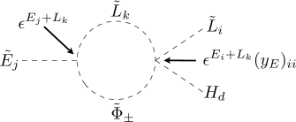
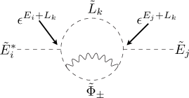
Figure 1: Example diagram for the 2-loop generation of (δRRe)ijsubscriptsubscriptsuperscript𝛿𝑒𝑅𝑅𝑖𝑗(\delta^{e}_{RR})_{ij}. L~i,E~isubscript~𝐿𝑖subscript~𝐸𝑖\tilde{L}_{i},\tilde{E}_{i} denotes the scalar components of the superfields Li,Eisubscript𝐿𝑖subscript𝐸𝑖L_{i},E_{i} and Φ~±subscript~Φplus-or-minus\tilde{\Phi}_{\pm} denotes the scalar mass eigenstates of the messengers.
Refer to caption
Figure 2: Example diagram for the 1-loop generation of (δLRe)ijsubscriptsubscriptsuperscript𝛿𝑒𝐿𝑅𝑖𝑗(\delta^{e}_{LR})_{ij} in the fermion mass basis.

We conclude this section with a discussion of the general structure of the flavor suppression in these terms. First of all, note that LL and RR mass insertions are suppressed by powers of the spurion that are the sum of U(1) charges, in contrast to the leading order terms allowed by the symmetry that have powers given by charge differences. The origin of this suppression is due to the fact that the U(1)𝑈1U(1) controls soft terms only indirectly via the messenger sector, which in turn generates soft terms only at loop level, thus leading to a double suppression by small couplings. As can be seen e.g. in Eq. (30) and the corresponding 2-loop diagram for δRResubscriptsuperscript𝛿𝑒𝑅𝑅\delta^{e}_{RR} in Fig. 1, this suppression can be split into two parts, one given by the sum of charges of the external sfermions and the second by (twice) the charge of the field that runs in the loop together with the messenger. As we will discuss later on, the first suppression is exactly the same as in SUSY Partial Compositeness, while the second can lead to a further suppression by powers of yτsubscript𝑦𝜏y_{\tau}.

Turning to LR mass insertions, again the loop origin implies a much stronger suppression than the leading order term ϵLi+Ejsuperscriptitalic-ϵsubscript𝐿𝑖subscript𝐸𝑗\epsilon^{L_{i}+E_{j}} respecting the U(1)𝑈1U(1) symmetry, see Fig. 2. This suppression is partially due to the alignment to Yukawas in the pure LR term, which potentially can be avoided in the effective LR terms at the price of an additional suppression by powers of yτsubscript𝑦𝜏y_{\tau}. This is also the only way in which phases can arise in the diagonal elements, since the pure LR term is always the product of a hermitian and a real diagonal matrix.

4 Flavor Phenomenology

LFV Process Present Bound Future Sensitivity
μeγ𝜇𝑒𝛾\mu\to e\gamma 5.7×10135.7superscript10135.7\times 10^{-13} [39] 6×10¹⁴absent6superscript1014\approx 6\times 10^{-14} [40]
μ3e𝜇3𝑒\mu\to 3e 1.0×10121.0superscript10121.0\times 10^{-12}[41] 1016absentsuperscript1016\approx 10^{-16} [42]
μsuperscript𝜇\mu^{-} Au \to esuperscript𝑒e^{-} Au 7.0×10137.0superscript10137.0\times 10^{-13} [43] ???
μsuperscript𝜇\mu^{-} Ti \to esuperscript𝑒e^{-} Ti 4.3×10124.3superscript10124.3\times 10^{-12} [44] ???
μsuperscript𝜇\mu^{-} Al \to esuperscript𝑒e^{-} Al - 1016absentsuperscript1016\approx 10^{-16} [45, 46]
Electron EDM Present Bound Future Sensitivity
de(ecm)subscript𝑑𝑒ecmd_{e}({\rm e~{}cm}) 8.7×10298.7superscript10298.7\times 10^{-29} [47] ???
Table 1: Current experimental bounds and future sensitivities for some low-energy LFV observables and the electron EDM.

We are now ready to discuss the lepton flavor phenomenology of the FGM model, which includes LFV processes with an underlying μe𝜇𝑒\mu\to e transition, the electron EDM desubscript𝑑𝑒d_{e} and the anomalous magnetic moment of the muon aμ(g2)/2subscript𝑎𝜇𝑔22a_{\mu}\equiv(g-2)/2. The current experimental bounds and future sensitivities for some of the most relevant LFV channels and for desubscript𝑑𝑒d_{e} are reported in Table 1. On the other hand, aμsubscript𝑎𝜇a_{\mu} currently shows a discrepancy between the SM prediction and the experimental value [48, 49, 50, 51]

Δaμ=aμEXPaμSM=2.90(90)×109.Δsubscript𝑎𝜇superscriptsubscript𝑎𝜇EXPsuperscriptsubscript𝑎𝜇SM2.9090superscript109\Delta a_{\mu}=a_{\mu}^{\scriptscriptstyle\rm EXP}-a_{\mu}^{\scriptscriptstyle\rm SM}=2.90(90)\times 10^{-9}\,. (33)

One of the goals of the present paper is to investigate whether it is possible to explain this anomaly in our model while being compatible with LFV and EDM bounds.

Concerning LFV processes, hereafter we focus only on μeγ𝜇𝑒𝛾\mu\to e\gamma since it represents the best probe of our scenario. The branching ratio of μeγ𝜇𝑒𝛾\mu\to e\gamma is defined as

BR(μeγ)=48π3αGF2(|AL21|2+|AR21|2),BR𝜇𝑒𝛾48superscript𝜋3𝛼subscriptsuperscript𝐺2𝐹superscriptsubscriptsuperscript𝐴21𝐿2superscriptsubscriptsuperscript𝐴21𝑅2\displaystyle{\rm BR}(\mu\to e\gamma)=\frac{48\pi^{3}\alpha}{G^{2}_{F}}\left(\left|A^{21}_{L}\right|^{2}+\left|A^{21}_{R}\right|^{2}\right), (34)

where the amplitudes AL21subscriptsuperscript𝐴21𝐿A^{21}_{L} and AR21subscriptsuperscript𝐴21𝑅A^{21}_{R}, in the limit of M1=M2=μ=m~L=m~R=m~subscript𝑀1subscript𝑀2𝜇subscript~𝑚𝐿subscript~𝑚𝑅~𝑚M_{1}=M_{2}=\mu=\tilde{m}_{L}=\tilde{m}_{R}=\tilde{m} and keeping only tanβ𝛽\tan\beta enhanced terms,666We will eventually prefer low values for tanβ𝛽\tan\beta (5less-than-or-similar-toabsent5\lesssim 5). For the numerical analysis later on one has therefore to take into account all contributions, which are collected in the Appendix. At this point we are rather interested in keeping the formulae simple and just give order-of-magnitude estimates. read

AL21subscriptsuperscript𝐴21𝐿\displaystyle A^{21}_{L} =\displaystyle= 4α2+5αY240πtanβm~2(δLLe)21+αY48π(m~mμ)1m~2(δLRe)12,4subscript𝛼25subscript𝛼𝑌240𝜋𝛽superscript~𝑚2subscriptsuperscriptsubscript𝛿𝐿𝐿𝑒21subscript𝛼𝑌48𝜋~𝑚subscript𝑚𝜇1superscript~𝑚2subscriptsuperscriptsuperscriptsubscript𝛿𝐿𝑅𝑒12\displaystyle\frac{4\alpha_{2}+5\alpha_{Y}}{240\pi}~{}\frac{\tan\beta}{{\tilde{m}}^{2}}~{}(\delta_{LL}^{e})_{21}+\frac{\alpha_{Y}}{48\pi}\left(\frac{{\tilde{m}}}{m_{\mu}}\right)~{}\frac{1}{{\tilde{m}}^{2}}~{}(\delta_{LR}^{e})^{*}_{12}\,, (35)
AR21subscriptsuperscript𝐴21𝑅\displaystyle A^{21}_{R} =\displaystyle= αY240πtanβm~2(δRRe)21+αY48π(m~mμ)1m~2(δLRe)21.subscript𝛼𝑌240𝜋𝛽superscript~𝑚2subscriptsuperscriptsubscript𝛿𝑅𝑅𝑒21subscript𝛼𝑌48𝜋~𝑚subscript𝑚𝜇1superscript~𝑚2subscriptsuperscriptsubscript𝛿𝐿𝑅𝑒21\displaystyle-\frac{\alpha_{Y}}{240\pi}~{}\frac{\tan\beta}{{\tilde{m}}^{2}}~{}(\delta_{RR}^{e})_{21}+\frac{\alpha_{Y}}{48\pi}\left(\frac{{\tilde{m}}}{m_{\mu}}\right)~{}\frac{1}{{\tilde{m}}^{2}}~{}(\delta_{LR}^{e})_{21}\,. (36)

Notice that in the above amplitudes we have kept only single MI effects since they are dominant in our scenarios. The expressions for ΔaμΔsubscript𝑎𝜇\Delta a_{\mu} and desubscript𝑑𝑒d_{e} are well approximated by

ΔaμΔsubscript𝑎𝜇\displaystyle\Delta a_{\mu} =\displaystyle= 5α2+αY48πmμ2m~2tanβ,5subscript𝛼2subscript𝛼𝑌48𝜋subscriptsuperscript𝑚2𝜇superscript~𝑚2𝛽\displaystyle\frac{5\alpha_{2}+\alpha_{Y}}{48\pi}\frac{m^{2}_{\mu}}{{\tilde{m}}^{2}}\tan\beta\,, (37)
deesubscript𝑑𝑒𝑒\displaystyle\frac{d_{e}}{e} =\displaystyle= αY120πmτm~2tanβIm[(δLLe)13(δRRe)31].subscript𝛼𝑌120𝜋subscript𝑚𝜏superscript~𝑚2𝛽Imdelimited-[]subscriptsuperscriptsubscript𝛿𝐿𝐿𝑒13subscriptsuperscriptsubscript𝛿𝑅𝑅𝑒31\displaystyle\frac{\alpha_{Y}}{120\pi}\frac{m_{\tau}}{{\tilde{m}}^{2}}\tan\beta~{}{\rm Im}[(\delta_{LL}^{e})_{13}(\delta_{RR}^{e})_{31}]\,. (38)

In order to highlight the relevant effects, we now provide some numerical estimates for the above observables outlining also their possible correlations. We find that

BR(μeγ)BR𝜇𝑒𝛾\displaystyle{\rm BR}(\mu\to e\gamma) \displaystyle\approx 3×10¹⁴(200GeVm~)4tan2β(|(δLLe)21|104)2,3superscript1014superscript200GeV~𝑚4superscript2𝛽superscriptsubscriptsuperscriptsubscript𝛿𝐿𝐿𝑒21superscript1042\displaystyle 3\times 10^{-14}\left(\frac{200~{}{\rm GeV}}{{\tilde{m}}}\right)^{4}\tan^{2}\beta~{}\left(\frac{|(\delta_{LL}^{e})_{21}|}{10^{-4}}\right)^{2}\,, (39)
ΔaμΔsubscript𝑎𝜇\displaystyle\Delta a_{\mu} \displaystyle\approx 3×10¹⁰(200GeVm~)2tanβ,3superscript1010superscript200GeV~𝑚2𝛽\displaystyle 3\times 10^{-10}\left(\frac{200~{}{\rm GeV}}{{\tilde{m}}}\right)^{2}\tan\beta\,, (40)
|de|subscript𝑑𝑒\displaystyle|d_{e}| \displaystyle\approx 2×1029(200GeVm~)2tanβ|Im[(δLLe)13(δRRe)31]106|ecm.2superscript1029superscript200GeV~𝑚2𝛽Imdelimited-[]subscriptsuperscriptsubscript𝛿𝐿𝐿𝑒13subscriptsuperscriptsubscript𝛿𝑅𝑅𝑒31superscript106𝑒cm\displaystyle 2\times 10^{-29}\left(\frac{200~{}{\rm GeV}}{{\tilde{m}}}\right)^{2}\tan\beta~{}\left|\frac{{\rm Im}[(\delta_{LL}^{e})_{13}(\delta_{RR}^{e})_{31}]}{10^{-6}}\right|e{\rm~{}cm}\,. (41)

Making the correlations among BR(μeγ)𝜇𝑒𝛾(\mu\to e\gamma), ΔaμΔsubscript𝑎𝜇\Delta a_{\mu} and desubscript𝑑𝑒d_{e} more explicit, it turns out that

BR(μeγ)BR𝜇𝑒𝛾\displaystyle{\rm BR}(\mu\to e\gamma) \displaystyle\approx 3×10¹³(Δaμ109)2(|(δLLe)21|104)2,3superscript1013superscriptΔsubscript𝑎𝜇superscript1092superscriptsubscriptsuperscriptsubscript𝛿𝐿𝐿𝑒21superscript1042\displaystyle 3\times 10^{-13}\left(\frac{\Delta a_{\mu}}{10^{-9}}\right)^{2}\left(\frac{|(\delta_{LL}^{e})_{21}|}{10^{-4}}\right)^{2}\,, (42)
|de|subscript𝑑𝑒\displaystyle|d_{e}| \displaystyle\approx 7×1029(Δaμ109)|Im[(δLLe)13(δRRe)31]106|ecm.7superscript1029Δsubscript𝑎𝜇superscript109Imdelimited-[]subscriptsuperscriptsubscript𝛿𝐿𝐿𝑒13subscriptsuperscriptsubscript𝛿𝑅𝑅𝑒31superscript106𝑒cm\displaystyle 7\times 10^{-29}\left(\frac{\Delta a_{\mu}}{10^{-9}}\right)\left|\frac{{\rm Im}[(\delta_{LL}^{e})_{13}(\delta_{RR}^{e})_{31}]}{10^{-6}}\right|e{\rm~{}cm}\,. (43)

Eqs. (39-41) deserve few comments:

  • In both flavor models we have considered, the dominant contribution to BR(μeγ)𝜇𝑒𝛾(\mu\to e\gamma) stems from AL21subscriptsuperscript𝐴21𝐿A^{21}_{L}, in particular from the tanβ𝛽\tan\beta-enhanced term proportional to (δLLe)21subscriptsuperscriptsubscript𝛿𝐿𝐿𝑒21(\delta_{LL}^{e})_{21}, due to smaller flavor hierarchies in the left-handed lepton sector.

  • The dominant μeγ𝜇𝑒𝛾\mu\to e\gamma amplitude grows with tanβ𝛽\tan\beta as AL21(δLLe)21tanβtan3βsimilar-tosubscriptsuperscript𝐴21𝐿subscriptsuperscriptsubscript𝛿𝐿𝐿𝑒21𝛽similar-tosuperscript3𝛽A^{21}_{L}\sim(\delta_{LL}^{e})_{21}\tan\beta\sim\tan^{3}\beta, since (δLLe)21yτ2104tan2βsimilar-tosubscriptsuperscriptsubscript𝛿𝐿𝐿𝑒21subscriptsuperscript𝑦2𝜏superscript104superscript2𝛽(\delta_{LL}^{e})_{21}\sim y^{2}_{\tau}\approx 10^{-4}\tan^{2}\beta, which implies that AL21subscriptsuperscript𝐴21𝐿A^{21}_{L} is very efficiently suppressed for relatively low tanβ𝛽\tan\beta. As a result, the very stringent experimental bound on BR(μeγ)𝜇𝑒𝛾(\mu\to e\gamma) might be fulfilled even for a light spectrum m~200similar-to~𝑚200{\tilde{m}}\sim 200~{}GeV provided tanβ1similar-to𝛽1\tan\beta\sim 1.

  • The electron EDM can be induced at the leading order only through the effective MI of Eq. (32) and it turns out that detan5βsimilar-tosubscript𝑑𝑒superscript5𝛽d_{e}\sim\tan^{5}\beta. Therefore desubscript𝑑𝑒d_{e} is well under control for low tanβ𝛽\tan\beta values, analogously to BR(μeγ)𝜇𝑒𝛾(\mu\to e\gamma).

  • The aμsubscript𝑎𝜇a_{\mu} anomaly can be accounted for while satisfying the stringent bounds from BR(μeγ)𝜇𝑒𝛾(\mu\to e\gamma) and desubscript𝑑𝑒d_{e}, only provided that the relevant flavor mixing angles are suppressed at the level of (δLLe)21104less-than-or-similar-tosubscriptsuperscriptsubscript𝛿𝐿𝐿𝑒21superscript104(\delta_{LL}^{e})_{21}\lesssim 10^{-4} and (δLLe)13(δRRe)31106less-than-or-similar-tosubscriptsuperscriptsubscript𝛿𝐿𝐿𝑒13subscriptsuperscriptsubscript𝛿𝑅𝑅𝑒31superscript106(\delta_{LL}^{e})_{13}(\delta_{RR}^{e})_{31}\lesssim 10^{-6}.

In order to quantify the above considerations, we specialize now to the U(1)𝑈1U(1) flavor models that have been introduced in the previous section: the anarchical and the hierarchical models. The predictions of other scenarios discussed in Refs.[10, 11], fall in between the ones we discuss here. In these two models, the relevant MIs entering the predictions of BR(μeγ)𝜇𝑒𝛾(\mu\to e\gamma) and desubscript𝑑𝑒d_{e} are estimated as:

  • Anarchy

    (δLLe)21subscriptsuperscriptsubscript𝛿𝐿𝐿𝑒21\displaystyle(\delta_{LL}^{e})_{21} κ6Nyτ2κ6×10⁴Ntan2β,absent𝜅6𝑁subscriptsuperscript𝑦2𝜏𝜅6superscript104𝑁superscript2𝛽\displaystyle\approx\kappa\frac{6}{N}~{}y^{2}_{\tau}\approx\kappa\frac{6\times 10^{-4}}{N}\tan^{2}\beta,
    (δLLe)13(δRRe)31subscriptsuperscriptsubscript𝛿𝐿𝐿𝑒13subscriptsuperscriptsubscript𝛿𝑅𝑅𝑒31\displaystyle(\delta_{LL}^{e})_{13}(\delta_{RR}^{e})_{31} κ200N2yτ4ϵA3κ2×10⁸N2(ϵA0.2)3tan4β.absentsuperscript𝜅200superscript𝑁2subscriptsuperscript𝑦4𝜏superscriptsubscriptitalic-ϵ𝐴3superscript𝜅2superscript108superscript𝑁2superscriptsubscriptitalic-ϵ𝐴0.23superscript4𝛽\displaystyle\approx\kappa^{\prime}\frac{200}{N^{2}}~{}y^{4}_{\tau}\epsilon_{A}^{3}\approx\kappa^{\prime}\frac{2\times 10^{-8}}{N^{2}}\left(\frac{\epsilon_{A}}{0.2}\right)^{3}\tan^{4}\beta\,. (44)
  • Hierarchy

    (δLLe)21subscriptsuperscriptsubscript𝛿𝐿𝐿𝑒21\displaystyle(\delta_{LL}^{e})_{21} κ6Nyτ2ϵH3κ2×10⁵Ntan2β(ϵH0.3)3,absent𝜅6𝑁subscriptsuperscript𝑦2𝜏subscriptsuperscriptitalic-ϵ3𝐻𝜅2superscript105𝑁superscript2𝛽superscriptsubscriptitalic-ϵ𝐻0.33\displaystyle\approx\kappa\frac{6}{N}~{}y^{2}_{\tau}\epsilon^{3}_{H}\approx\kappa\frac{2\times 10^{-5}}{N}\tan^{2}\beta\left(\frac{\epsilon_{H}}{0.3}\right)^{3},
    (δLLe)13(δRRe)31subscriptsuperscriptsubscript𝛿𝐿𝐿𝑒13subscriptsuperscriptsubscript𝛿𝑅𝑅𝑒31\displaystyle(\delta_{LL}^{e})_{13}(\delta_{RR}^{e})_{31} κ200N2yτ4ϵH7κ4×10¹⁰N2(ϵH0.3)7tan4β.absentsuperscript𝜅200superscript𝑁2subscriptsuperscript𝑦4𝜏superscriptsubscriptitalic-ϵ𝐻7superscript𝜅4superscript1010superscript𝑁2superscriptsubscriptitalic-ϵ𝐻0.37superscript4𝛽\displaystyle\approx\kappa^{\prime}\frac{200}{N^{2}}~{}y^{4}_{\tau}\epsilon_{H}^{7}\approx\kappa^{\prime}\frac{4\times 10^{-10}}{N^{2}}\left(\frac{\epsilon_{H}}{0.3}\right)^{7}\tan^{4}\beta\,. (45)

where we have used Eqs. (13), (28) assuming an intermediate mediation scale M1010GeVsimilar-to𝑀superscript1010GeVM\sim 10^{10}\,{\rm GeV}. Moreover, we have explicitly included the dependence on the unknown 𝒪(1)𝒪1{\cal O}(1) coefficients parameterized through κ𝜅\kappa and κsuperscript𝜅\kappa^{\prime} that are defined as

κ𝜅\displaystyle\kappa κ23κ13a332,absentsubscript𝜅23superscriptsubscript𝜅13superscriptsubscript𝑎332\displaystyle\equiv\frac{\kappa_{23}\kappa_{13}^{*}}{a_{33}^{2}}\,, κsuperscript𝜅\displaystyle\kappa^{\prime} κ13κ31κ332a334.absentsubscript𝜅13subscript𝜅31superscriptsubscript𝜅33absent2superscriptsubscript𝑎334\displaystyle\equiv\frac{\kappa_{13}\kappa_{31}\kappa_{33}^{*2}}{a_{33}^{4}}. (46)

A prominent feature emerging from Eqs. (44)-(45) is the sensitivity of the MIs to the number of messenger N𝑁N, since the diagonal sfermion masses are dominated by the MGM contribution proportional to N𝑁N. We finally get for the μeγ𝜇𝑒𝛾\mu\to e\gamma branching ratio

BR(μeγ)BR𝜇𝑒𝛾\displaystyle{\rm BR}(\mu\to e\gamma) tan6β(κN)2(200GeVm~)4×{1×10¹²Anarchy9×1016Hierarchyabsentsuperscript6𝛽superscript𝜅𝑁2superscript200GeV~𝑚4cases1superscript1012Anarchy9superscript1016Hierarchy\displaystyle\approx\tan^{6}\beta\left(\frac{\kappa}{N}\right)^{2}\left(\frac{200~{}{\rm GeV}}{{\tilde{m}}}\right)^{4}\times\begin{cases}1\times 10^{-12}&{\rm Anarchy}\\ 9\times 10^{-16}&{\rm Hierarchy}\end{cases} (47)
tan4β(κN)2(Δaμ109)2×{1×10¹¹Anarchy9×1015Hierarchyabsentsuperscript4𝛽superscript𝜅𝑁2superscriptΔsubscript𝑎𝜇superscript1092cases1superscript1011Anarchy9superscript1015Hierarchy\displaystyle\approx\tan^{4}\beta\left(\frac{\kappa}{N}\right)^{2}\left(\frac{\Delta a_{\mu}}{10^{-9}}\right)^{2}\times\begin{cases}1\times 10^{-11}&{\rm Anarchy}\\ 9\times 10^{-15}&{\rm Hierarchy}\end{cases} (48)

and the eEDM

|de|subscript𝑑𝑒\displaystyle|d_{e}| tan5β(κN2)(200GeVm~)2ecm×{4×1031Anarchy1×1032Hierarchyabsentsuperscript5𝛽superscript𝜅superscript𝑁2superscript200GeV~𝑚2𝑒cmcases4superscript1031Anarchy1superscript1032Hierarchy\displaystyle\approx\tan^{5}\beta\left(\frac{\kappa^{\prime}}{N^{2}}\right)\left(\frac{200~{}{\rm GeV}}{{\tilde{m}}}\right)^{2}e{\rm~{}cm}\,\times\begin{cases}4\times 10^{-31}&{\rm Anarchy}\\ 1\times 10^{-32}&{\rm Hierarchy}\end{cases} (49)
tan4β(κN2)(Δaμ109)ecm×{1×1030Anarchy3×1032Hierarchy.absentsuperscript4𝛽superscript𝜅superscript𝑁2Δsubscript𝑎𝜇superscript109𝑒cmcases1superscript1030Anarchy3superscript1032Hierarchy\displaystyle\approx\tan^{4}\beta\left(\frac{\kappa^{\prime}}{N^{2}}\right)\left(\frac{\Delta a_{\mu}}{10^{-9}}\right)e{\rm~{}cm}\times\begin{cases}1\times 10^{-30}&{\rm Anarchy}\\ 3\times 10^{-32}&{\rm Hierarchy}\,.\end{cases} (50)

Reformulating the constraint from μeγ𝜇𝑒𝛾\mu\to e\gamma as a bound on the SUSY scale gives approximately

m~200GeVtan3/2βκN(BR(μeγ)5.7×1013)1/4×{1Anarchy0.2Hierarchy.greater-than-or-equivalent-to~𝑚200GeVsuperscript32𝛽𝜅𝑁superscriptBR𝜇𝑒𝛾5.7superscript101314cases1Anarchy0.2Hierarchy\displaystyle\frac{\tilde{m}}{200\,{\rm GeV}}\gtrsim\tan^{3/2}\beta\sqrt{\frac{\kappa}{N}}\left(\frac{{\rm BR}(\mu\to e\gamma)}{5.7\times 10^{-13}}\right)^{1/4}\times\begin{cases}1&{\rm Anarchy}\\ 0.2&{\rm Hierarchy}\,.\end{cases} (51)
Refer to caption
Refer to caption
Refer to caption
Refer to caption
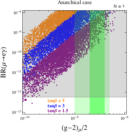
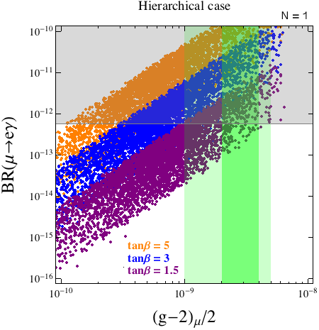
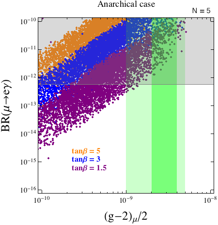
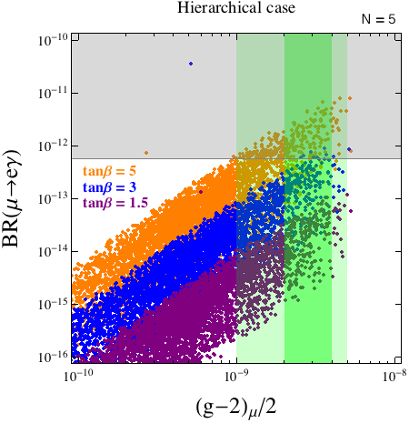
Figure 3: Predictions for BR(μeγ)𝜇𝑒𝛾(\mu\to e\gamma) vs. ΔaμΔsubscript𝑎𝜇\Delta a_{\mu} for different values of tanβ𝛽\tan\beta: purple, blue and orange dots correspond to tanβ=1.5,3,5𝛽1.535\tan\beta=1.5,3,5, respectively. The plots on the left (right) refer to the anarchical (hierarchical) case. For the upper (lower) plots the number of messenger is set to N=1(5)𝑁15N=1~{}(5).

Having outlined the expected behaviors and main features of flavor observables within our FGM setup supplemented by U(1)𝑈1U(1) flavor models, we are ready now to perform a complete numerical analysis.
Refer to caption
Refer to caption
Refer to caption
Refer to caption
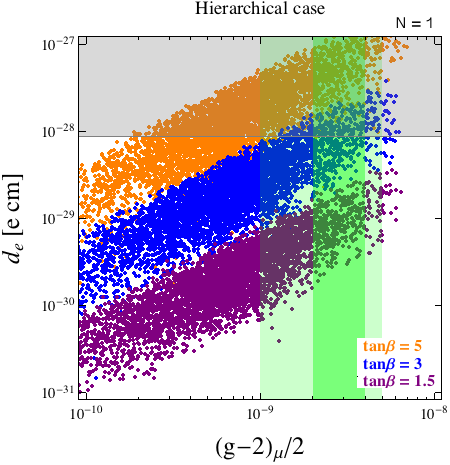
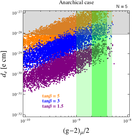
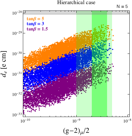
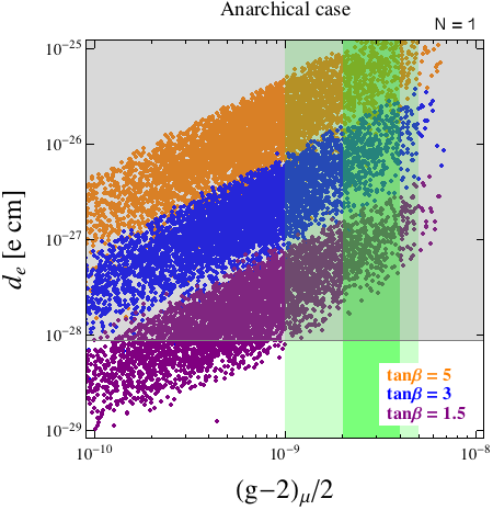
Figure 4: The same scenarios as in Fig. 3 for desubscript𝑑𝑒d_{e} vs. ΔaμΔsubscript𝑎𝜇\Delta a_{\mu}.
Refer to caption
Refer to caption
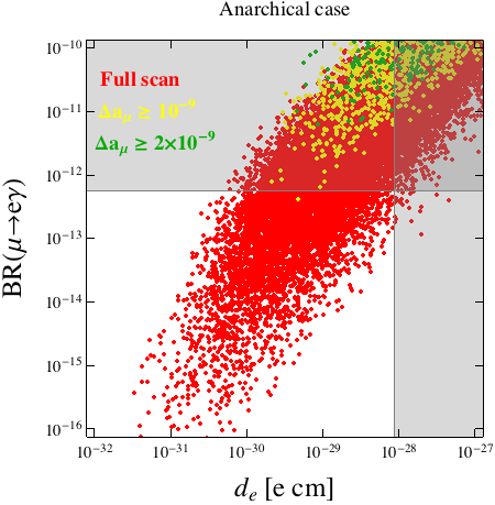
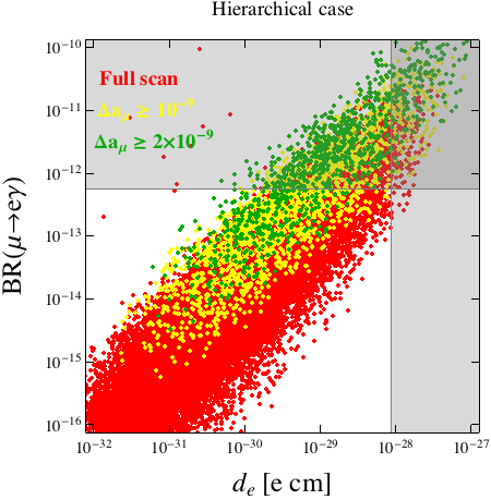
Figure 5: Predictions for BR(μeγ)𝜇𝑒𝛾(\mu\to e\gamma) vs. desubscript𝑑𝑒d_{e} for the anarchical (left) and hierarchical (right) cases. Yellow (green) points correspond to Δaμ109Δsubscript𝑎𝜇superscript109\Delta a_{\mu}\geq 10^{-9} (2×1092superscript1092\times 10^{-9}).

In Fig. 3, we show the predictions for BR(μeγ)𝜇𝑒𝛾(\mu\to e\gamma) vs. ΔaμΔsubscript𝑎𝜇\Delta a_{\mu} for different values of tanβ𝛽\tan\beta: purple, blue and orange dots correspond to tanβ=1.5,3,5𝛽1.535\tan\beta=1.5,3,5, respectively. The plots on the left (right) refer to the anarchical (hierarchical) case. For the upper (lower) plots the number of messenger is set to N=1(5)𝑁15N=1~{}(5). In Fig. 4, we show the analogous plots for desubscript𝑑𝑒d_{e} vs. ΔaμΔsubscript𝑎𝜇\Delta a_{\mu}. In the scan we have varied the unknown 𝒪(1)𝒪1\mathcal{O}(1) coefficients κ,κ𝜅superscript𝜅\kappa,\kappa^{\prime} for the MIs in the range (0.3,1.5)0.31.5(0.3,1.5). The other parameters were varied in the following ranges:

106GeVM1015GeV,100GeVm~E(M)1TeV,100GeVμμmax,formulae-sequencesuperscript106GeV𝑀superscript1015GeV100GeVsubscript~𝑚𝐸𝑀1TeV100GeV𝜇subscript𝜇max\displaystyle 10^{6}~{}{\rm GeV}\leq M\leq 10^{15}~{}{\rm GeV},~{}~{}100~{}{\rm GeV}\leq\tilde{m}_{E}(M)\leq 1~{}{\rm TeV},~{}~{}100~{}{\rm GeV}\leq\mu\leq\mu_{\rm max}, (52)

where μmaxm~τLm~τR/(mτtanβ)subscript𝜇maxsubscript~𝑚subscript𝜏𝐿subscript~𝑚subscript𝜏𝑅subscript𝑚𝜏𝛽\mu_{\rm max}\equiv\tilde{m}_{\tau_{L}}\tilde{m}_{\tau_{R}}/(m_{\tau}\tan\beta) is the maximal value giving a non-tachyonic stau. In the plots, the gray shaded regions are excluded by the current bounds from μeγ𝜇𝑒𝛾\mu\to e\gamma or desubscript𝑑𝑒d_{e} reported in Table 1, while the green (dark green) area approximately corresponds to values of ΔaμΔsubscript𝑎𝜇\Delta a_{\mu} lowering the discrepancy below the 2σ𝜎\sigma (1σ𝜎\sigma) level.

A direct comparison of the bounds and the discovery potential of μeγ𝜇𝑒𝛾\mu\to e\gamma and desubscript𝑑𝑒d_{e} is shown in Fig. 5, where we plot the result of a random variation of the full set of parameters for the anarchical (left) and hierarchical (right) cases:

106GeVM1015GeV,100GeVm~E(M)2TeV,100GeVμμmax,formulae-sequencesuperscript106GeV𝑀superscript1015GeV100GeVsubscript~𝑚𝐸𝑀2TeV100GeV𝜇subscript𝜇max\displaystyle 10^{6}~{}{\rm GeV}\leq M\leq 10^{15}~{}{\rm GeV},~{}~{}100~{}{\rm GeV}\leq\tilde{m}_{E}(M)\leq 2~{}{\rm TeV},~{}~{}100~{}{\rm GeV}\leq\mu\leq\mu_{\rm max},
1N5,1.5tanβ5,0.3κ,κ1.5.formulae-sequence1𝑁51.5𝛽5formulae-sequence0.3𝜅superscript𝜅1.5\displaystyle 1\leq N\leq 5,\quad 1.5\leq\tan\beta\leq 5,\quad 0.3\leq\kappa,\kappa^{\prime}\leq 1.5. (53)

In addition, the yellow (green) points correspond to Δaμ109Δsubscript𝑎𝜇superscript109\Delta a_{\mu}\geq 10^{-9} (2×1092superscript1092\times 10^{-9}).

The main results emerging from our numerical analysis can be summarizes as follows:

  • In the anarchical scenario, it is very difficult if not impossible to explain the ΔaμΔsubscript𝑎𝜇\Delta a_{\mu} anomaly because of the strong bounds from both BR(μeγ)𝜇𝑒𝛾(\mu\to e\gamma) and desubscript𝑑𝑒d_{e} (see left panels of Figs. 3-5). The latter observables have a comparable sensitivity to the scenario in question and might reach experimentally visible values even for SUSY masses far beyond the LHC reach in the multi-TeV regime. As already discussed, BR(μeγ)𝜇𝑒𝛾(\mu\to e\gamma) and desubscript𝑑𝑒d_{e} grow fast with tanβ𝛽\tan\beta (like tan6βsuperscript6𝛽\tan^{6}\beta and tan5βsuperscript5𝛽\tan^{5}\beta, respectively) and are both suppressed by increasing N𝑁N. As a result, the scenario with low tanβ𝛽\tan\beta and N=5𝑁5N=5 (we remind that for low mediation scales perturbativity requires N5less-than-or-similar-to𝑁5N\lesssim 5) is the most favorable scenario, as clearly shown in Figs. 3 and 4.

  • The hierarchical scenario easily offers the possibility to explain the ΔaμΔsubscript𝑎𝜇\Delta a_{\mu} anomaly while satisfying the limits on BR(μeγ)𝜇𝑒𝛾(\mu\to e\gamma) and desubscript𝑑𝑒d_{e} (right panels of Figs. 3-5). This happens thanks to the stronger suppression of the flavor mixing angles compared to the anarchical case. On the other hand, all the others considerations made above for the anarchical case apply here as well.

  • μeγ𝜇𝑒𝛾\mu\to e\gamma and desubscript𝑑𝑒d_{e} have comparable sensitivities, but μeγ𝜇𝑒𝛾\mu\to e\gamma is currently more constraining, as we can see from Fig. 5. Interestingly, an improvement of the sensitivity by one or two orders of magnitude would make the electron EDM the most powerful probe of FGM scenarios especially in case of heavy superpartners, corresponding to the red points in Fig. 5. This is a consequence of the slower decoupling of desubscript𝑑𝑒d_{e} with respect to the NP scale: dem~2similar-tosubscript𝑑𝑒superscript~𝑚2d_{e}\sim{\tilde{m}}^{-2}, while BR(μeγ)m~4similar-to𝜇𝑒𝛾superscript~𝑚4(\mu\to e\gamma)\sim{\tilde{m}}^{-4}.

  • Given the expected future sensitivities to the μe𝜇𝑒\mu\to e transitions reported in Table 1 and the following approximate relations among different decay modes:

    BR(μeee)BR𝜇𝑒𝑒𝑒\displaystyle{{\rm BR}(\mu\to eee)} similar-to-or-equals\displaystyle\simeq α3π(logmμ2me23)BR(μeγ),𝛼3𝜋subscriptsuperscript𝑚2𝜇subscriptsuperscript𝑚2𝑒3BR𝜇𝑒𝛾\displaystyle\frac{\alpha}{3\pi}\bigg{(}\log\frac{m^{2}_{\mu}}{m^{2}_{e}}-3\bigg{)}{\rm BR}(\mu\to e\gamma)~{},
    CR(μein N)CR𝜇𝑒in N\displaystyle{\rm CR}(\mu\to e~{}\mbox{in N}) similar-to-or-equals\displaystyle\simeq α×BR(μeγ),𝛼BR𝜇𝑒𝛾\displaystyle\alpha\times{\rm BR}(\mu\to e\gamma)~{}, (54)

    we see that there are good prospects for a full test of the parameter space favored by ΔaμΔsubscript𝑎𝜇\Delta a_{\mu} at future experiments.

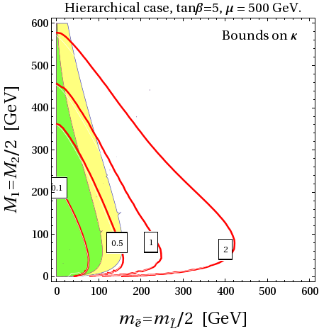
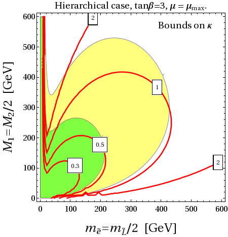
Let us now also show how the μeγ𝜇𝑒𝛾\mu\to e\gamma and desubscript𝑑𝑒d_{e} constraints appear in terms of the gaugino and slepton masses. For illustration purposes, we adopt a more general low-energy spectrum than the one predicted by MGM, which allows us to parameterize in a model-independent way possible distortions of the spectrum due to the full set of matter-messenger couplings studied in [25], including the other couplings in Eq. (4), as well as more generic SUSY breaking sectors, in the spirit of General Gauge Mediation [52]. In practice, we still use Eqs. (9-11) to set the off-diagonal entries but we treat slepton and gaugino masses as free parameters at low energy.
Refer to caption
Refer to caption
Figure 6: Bounds on the 𝒪(1)𝒪1\mathcal{O}(1) coefficient κ𝜅\kappa, see Eq. (46), from μeγ𝜇𝑒𝛾\mu\to e\gamma in the hierarchical scenario. For definiteness, we have assumed M2=2M1subscript𝑀22subscript𝑀1M_{2}=2M_{1}, m~L=2m~Esubscript~𝑚𝐿2subscript~𝑚𝐸\tilde{m}_{L}=2\tilde{m}_{E} and different choices of μ𝜇\mu and tanβ𝛽\tan\beta. The yellow (green) areas give Δaμ109Δsubscript𝑎𝜇superscript109\Delta a_{\mu}\geq 10^{-9} (2×1092superscript1092\times 10^{-9}).
Refer to caption
Refer to caption
Refer to caption
Refer to caption
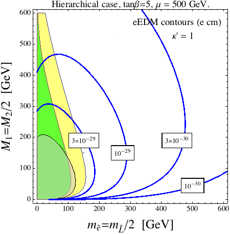
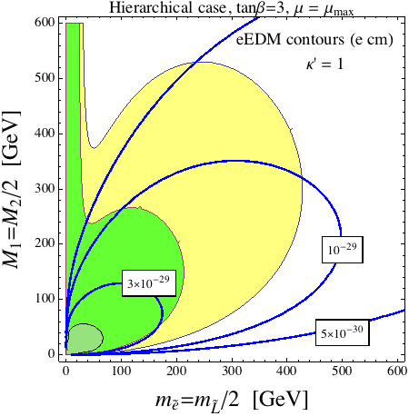
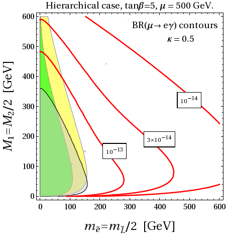
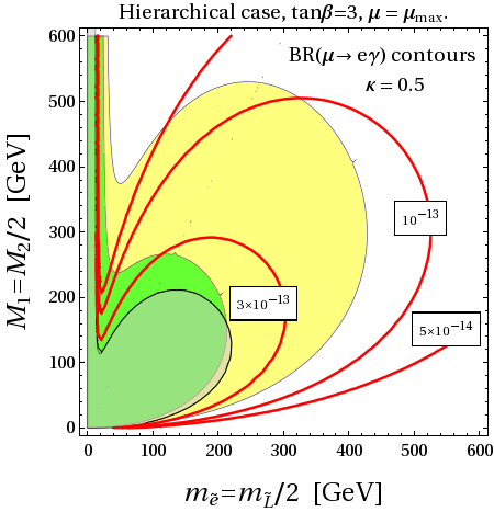
Figure 7: Contours of BR(μeγ𝜇𝑒𝛾\mu\to e\gamma) and desubscript𝑑𝑒d_{e} for the same choice of the parameters as in Fig. 6 and κ=0.5𝜅0.5\kappa=0.5, κ=1superscript𝜅1\kappa^{\prime}=1. The gray shaded regions are presently excluded by μeγ𝜇𝑒𝛾\mu\to e\gamma or desubscript𝑑𝑒d_{e}.

In Fig. 6, we show the current bounds on the 𝒪(1)𝒪1\mathcal{O}(1) coefficient κ𝜅\kappa, as defined in Eq. (46), from μeγ𝜇𝑒𝛾\mu\to e\gamma for different choices of μ𝜇\mu and tanβ𝛽\tan\beta in the hierarchical case. For definiteness, we fixed the relation among gauginos and slepton masses as follows: M2=2×M1subscript𝑀22subscript𝑀1M_{2}=2\times M_{1}, m~L=2×m~Esubscript~𝑚𝐿2subscript~𝑚𝐸\tilde{m}_{L}=2\times\tilde{m}_{E}. The yellow (green) areas give Δaμ109Δsubscript𝑎𝜇superscript109\Delta a_{\mu}\geq 10^{-9} (2×1092superscript1092\times 10^{-9}). As we can see, it is not necessary that the unknown coefficients conspire to provide an unnaturally small suppression, in order to take μeγ𝜇𝑒𝛾\mu\to e\gamma under control in the region favored by (g2)μsubscript𝑔2𝜇(g-2)_{\mu}.

In Fig. 7, we show contours of BR(μeγ𝜇𝑒𝛾\mu\to e\gamma) and desubscript𝑑𝑒d_{e} for the same choice of the parameters as above and the specific values κ=0.5𝜅0.5\kappa=0.5, κ=1superscript𝜅1\kappa^{\prime}=1, in order to illustrate the present bounds and the possible impact of the future experiments in terms of the masses of the SUSY particles in the game. In particular, the gray shaded regions are presently excluded by μeγ𝜇𝑒𝛾\mu\to e\gamma or desubscript𝑑𝑒d_{e}. Again, we see that a large contribution to (g2)μsubscript𝑔2𝜇(g-2)_{\mu} is perfectly compatible with the present bounds, but there are good prospects for a full test of the relevant parameter space in the future.

Besides the LEP constraints (corresponding to m~E,m~L,M2100GeVgreater-than-or-equivalent-tosubscript~𝑚𝐸subscript~𝑚𝐿subscript𝑀2100GeV\tilde{m}_{E},~{}\tilde{m}_{L},M_{2}\gtrsim 100~{}{\rm GeV}), the mass plane shown in the above plots is now challenged by searches for the electroweak production of SUSY particles performed by the LHC experiments, based on events with two or more leptons plus missing transverse momentum. The exact bounds are model dependent and their precise derivation is beyond the scope of the present study. Nevertheless, we briefly summarize here their possible impact.

Since we are considering scenarios with gauge-mediated SUSY breaking, the LSP is always a practically massless gravitino. The limits set by LHC searches then strongly depend on the nature and the life-time of the next to LSP (NLSP). In case the sleptons are lighter than the Bino, as it can occur even in MGM for large values of N𝑁N, each decay chain would end with the degenerate sleptons NLSP decaying into leptons and gravitino. If this decay occurs promptly (which requires low mediation scales, M106less-than-or-similar-to𝑀superscript106M\lesssim 10^{6} GeV), then the bounds from direct (Drell-Yan) slepton production translate to a limit on the mass of the right-handed (left-handed) sleptons at about 250 (300) GeV [53]. In case sleptons are long-lived compared to the detector scale, searches for charged tracks set a bound on degenerate slepton NLSP mass at about 400 GeV [54]. Interestingly, no searches performed so far constrain the intermediate case, featuring a disappearing track with a displaced vertex inside the detector, occurring for a wide range of the messenger scale, 106GeVM109GeVless-than-or-similar-tosuperscript106GeV𝑀less-than-or-similar-tosuperscript109GeV10^{6}~{}{\rm GeV}\lesssim M\lesssim 10^{9}~{}{\rm GeV} [55]. The above limits can be substantially relaxed if the Bino is lighter than the sleptons and escapes the detector, thus resembling searches within gravity mediation. In particular for a neutralino NLSP heavier than about 150 GeV, there is no constraint from direct slepton production [53].

The most stringent constraint would occur in the case of the hierarchy M1<m~L<M2subscript𝑀1subscript~𝑚𝐿subscript𝑀2M_{1}<\tilde{m}_{L}<M_{2} from Wino-like chargino/neutralino production followed by decays into on-shell sleptons/sneutrinos, with bounds up to 700 GeV on the Wino mass from multi-lepton plus missing energy searches [56]. However, such searches loose sensitivity if the mass splitting of the sleptons with either the Bino or the Wino gets small.

Comparing the limits reported above, with our plots in Fig. 6 and 7, we see that there is still room for a large SUSY contribution to aμsubscript𝑎𝜇a_{\mu}, at least at the 109superscript10910^{-9} level (yellow regions), especially if μ𝜇\mu approaches the maximal value μmaxm~τLm~τR/(mτtanβ)subscript𝜇maxsubscript~𝑚subscript𝜏𝐿subscript~𝑚subscript𝜏𝑅subscript𝑚𝜏𝛽\mu_{\rm max}\equiv\tilde{m}_{\tau_{L}}\tilde{m}_{\tau_{R}}/(m_{\tau}\tan\beta). This conclusion is supported by the results of Refs. [57, 58] where a systematic study of the LHC constraints on the parameter space favored by (g2)μsubscript𝑔2𝜇(g-2)_{\mu} has been presented.

5 Comparison with other models

In this section, we compare the peculiar flavor structure of FGM to other models that predict the parametric flavor suppression of soft terms. In particular, we consider U(1)𝑈1U(1) flavor models within SUGRA scenarios and models with SUSY Partial Compositeness (PC).

In those models the SUSY mediation scale ΛSsubscriptΛ𝑆\Lambda_{S} is assumed to be above the scale of flavor messengers ΛFsubscriptΛ𝐹\Lambda_{F}, so that the flavor structure of soft terms at the scale ΛFsubscriptΛ𝐹\Lambda_{F} is controlled entirely by the flavor dynamics at this scale, irrespectively of their structure at the scale ΛSsubscriptΛ𝑆\Lambda_{S}. In FGM the situation is reversed as the SUSY messenger scale ΛS=MsubscriptΛ𝑆𝑀\Lambda_{S}=M is below ΛFsubscriptΛ𝐹\Lambda_{F}. We stress that this setup is therefore complementary to the other scenarios, allowing also for very low SUSY mediation scales. All the unspecified dynamics of the flavor sector is imprinted in the matter-messenger couplings, just like Yukawas, and the full SUSY spectrum is totally calculable in terms of these couplings.

5.1 U(1)𝑈1U(1) and Gravity Mediation

In Gravity Mediation the natural expectation for soft terms at the flavor scale is given by the most general terms invariant under the symmetry using the flavon as a spurion. This gives for slepton mass insertions

(δLRe)ijAvdm~Lm~EϵLi+Ej,similar-tosubscriptsuperscriptsubscript𝛿𝐿𝑅𝑒𝑖𝑗𝐴subscript𝑣𝑑subscript~𝑚𝐿subscript~𝑚𝐸superscriptitalic-ϵsubscript𝐿𝑖subscript𝐸𝑗\displaystyle(\delta_{LR}^{e})_{ij}\sim\frac{Av_{d}}{\tilde{m}_{L}\tilde{m}_{E}}\epsilon^{L_{i}+E_{j}}\,, (55)
(δLLe)ijsubscriptsuperscriptsubscript𝛿𝐿𝐿𝑒𝑖𝑗\displaystyle(\delta_{LL}^{e})_{ij} ϵ|LiLj|,similar-toabsentsuperscriptitalic-ϵsubscript𝐿𝑖subscript𝐿𝑗\displaystyle\sim\epsilon^{|L_{i}-L_{j}|}\,, (δRRe)ijsubscriptsuperscriptsubscript𝛿𝑅𝑅𝑒𝑖𝑗\displaystyle(\delta_{RR}^{e})_{ij} ϵ|EiEj|.similar-toabsentsuperscriptitalic-ϵsubscript𝐸𝑖subscript𝐸𝑗\displaystyle\sim\epsilon^{|E_{i}-E_{j}|}\,. (56)

Focusing on the anarchical and hierarchical models of Section 3.1, the relevant MIs for BR(μeγ)𝜇𝑒𝛾(\mu\to e\gamma) and desubscript𝑑𝑒d_{e} are again (δLLe)21subscriptsuperscriptsubscript𝛿𝐿𝐿𝑒21(\delta_{LL}^{e})_{21} and (δLLe)13(δRRe)31subscriptsuperscriptsubscript𝛿𝐿𝐿𝑒13subscriptsuperscriptsubscript𝛿𝑅𝑅𝑒31(\delta_{LL}^{e})_{13}(\delta_{RR}^{e})_{31}, respectively. In the anarchic case we find:

  • Anarchy

    (δLLe)211,(δLLe)13(δRRe)31ϵA3,formulae-sequencesimilar-tosubscriptsuperscriptsubscript𝛿𝐿𝐿𝑒211similar-tosubscriptsuperscriptsubscript𝛿𝐿𝐿𝑒13subscriptsuperscriptsubscript𝛿𝑅𝑅𝑒31subscriptsuperscriptitalic-ϵ3𝐴\displaystyle(\delta_{LL}^{e})_{21}\sim 1\,,\qquad(\delta_{LL}^{e})_{13}(\delta_{RR}^{e})_{31}\sim\epsilon^{3}_{A}\,, (57)

    leading to the following predictions:

    BR(μeγ)BR𝜇𝑒𝛾\displaystyle{\rm BR}(\mu\to e\gamma) similar-to\displaystyle\sim 5×10¹³(10TeVm~)4tan2β,5superscript1013superscript10TeV~𝑚4superscript2𝛽\displaystyle 5\times 10^{-13}\left(\frac{10~{}{\rm TeV}}{{\tilde{m}}}\right)^{4}\tan^{2}\beta\,, (58)
    |de|subscript𝑑𝑒\displaystyle|d_{e}| similar-to\displaystyle\sim 7×1029(10TeVm~)2tanβecm.7superscript1029superscript10TeV~𝑚2𝛽𝑒cm\displaystyle 7\times 10^{-29}\left(\frac{10~{}{\rm TeV}}{{\tilde{m}}}\right)^{2}\tan\beta\,e{\rm\,cm}\,. (59)
  • Hierarchy

    (δLLe)21ϵH0.3,(δLLe)12(δRRe)21ϵH3,formulae-sequencesimilar-tosubscriptsuperscriptsubscript𝛿𝐿𝐿𝑒21subscriptitalic-ϵ𝐻similar-to0.3similar-tosubscriptsuperscriptsubscript𝛿𝐿𝐿𝑒12subscriptsuperscriptsubscript𝛿𝑅𝑅𝑒21subscriptsuperscriptitalic-ϵ3𝐻\displaystyle(\delta_{LL}^{e})_{21}\sim\epsilon_{H}\sim 0.3\,,\qquad(\delta_{LL}^{e})_{12}(\delta_{RR}^{e})_{21}\sim\epsilon^{3}_{H}\,, (60)

    where we took (δLLe)12(δRRe)21subscriptsuperscriptsubscript𝛿𝐿𝐿𝑒12subscriptsuperscriptsubscript𝛿𝑅𝑅𝑒21(\delta_{LL}^{e})_{12}(\delta_{RR}^{e})_{21} instead of (δLLe)13(δRRe)31subscriptsuperscriptsubscript𝛿𝐿𝐿𝑒13subscriptsuperscriptsubscript𝛿𝑅𝑅𝑒31(\delta_{LL}^{e})_{13}(\delta_{RR}^{e})_{31} since the contribution of the latter to the eEDM is smaller by a factor of (yτ/yμ)×ϵH40.1similar-tosubscript𝑦𝜏subscript𝑦𝜇subscriptsuperscriptitalic-ϵ4𝐻0.1(y_{\tau}/y_{\mu})\times\epsilon^{4}_{H}\sim 0.1 compared to that induced by (δLLe)12(δRRe)21subscriptsuperscriptsubscript𝛿𝐿𝐿𝑒12subscriptsuperscriptsubscript𝛿𝑅𝑅𝑒21(\delta_{LL}^{e})_{12}(\delta_{RR}^{e})_{21}. We therefore have the following predictions:

    BR(μeγ)BR𝜇𝑒𝛾\displaystyle{\rm BR}(\mu\to e\gamma) similar-to\displaystyle\sim 7×10¹³(5TeVm~)4tan2β(ϵH0.3)2,7superscript1013superscript5TeV~𝑚4superscript2𝛽superscriptsubscriptitalic-ϵ𝐻0.32\displaystyle 7\times 10^{-13}\left(\frac{5~{}{\rm TeV}}{{\tilde{m}}}\right)^{4}\tan^{2}\beta~{}\left(\frac{\epsilon_{H}}{0.3}\right)^{2}\,, (61)
    |de|subscript𝑑𝑒\displaystyle|d_{e}| similar-to\displaystyle\sim 6×1029(5TeVm~)2tanβecm.6superscript1029superscript5TeV~𝑚2𝛽𝑒cm\displaystyle 6\times 10^{-29}\left(\frac{5~{}{\rm TeV}}{{\tilde{m}}}\right)^{2}\tan\beta\,e{\rm\,cm}\,. (62)

As a result, single U(1)𝑈1U(1) flavor models with Gravity Mediation need sleptons well above the TeV scale, m~10TeV×tanβ(5TeV×tanβ)greater-than-or-equivalent-to~𝑚10TeV𝛽5TeV𝛽{\tilde{m}}\gtrsim 10~{}{\rm TeV}\times\sqrt{\tan\beta}~{}(5~{}{\rm TeV}\times\sqrt{\tan\beta}) in the anarchical (hierarchical) scenario. Note that the bounds on the SUSY spectrum in the quark sector, in particular from ϵKsubscriptitalic-ϵ𝐾\epsilon_{K}, are much stronger [28].

SUGRA U(1)𝑈1U(1) PC FGM U(1)𝑈1U(1)
m~meIm(δLR)11~𝑚subscript𝑚𝑒Imsubscriptsubscript𝛿𝐿𝑅11\frac{\tilde{m}}{m_{e}}{\rm Im}(\delta_{LR})_{11} 111 111 yτ4tβsuperscriptsubscript𝑦𝜏4subscript𝑡𝛽y_{\tau}^{4}t_{\beta}
m~mμ(δLR)12~𝑚subscript𝑚𝜇subscriptsubscript𝛿𝐿𝑅12\frac{\tilde{m}}{m_{\mu}}(\delta_{LR})_{12} ϵL1L2superscriptitalic-ϵsubscript𝐿1subscript𝐿2\epsilon^{L_{1}-L_{2}} ϵL1L2superscriptitalic-ϵsubscript𝐿1subscript𝐿2\epsilon^{L_{1}-L_{2}} yτ2ϵL1+L22L3superscriptsubscript𝑦𝜏2superscriptitalic-ϵsubscript𝐿1subscript𝐿22subscript𝐿3y_{\tau}^{2}\epsilon^{L_{1}+L_{2}-2L_{3}}
m~mμ(δLR)21~𝑚subscript𝑚𝜇subscriptsubscript𝛿𝐿𝑅21\frac{\tilde{m}}{m_{\mu}}(\delta_{LR})_{21} ϵE1E2superscriptitalic-ϵsubscript𝐸1subscript𝐸2\epsilon^{E_{1}-E_{2}} ϵE1E2superscriptitalic-ϵsubscript𝐸1subscript𝐸2\epsilon^{E_{1}-E_{2}} yτ2ϵE1E2+2L12L3superscriptsubscript𝑦𝜏2superscriptitalic-ϵsubscript𝐸1subscript𝐸22subscript𝐿12subscript𝐿3y_{\tau}^{2}\epsilon^{E_{1}-E_{2}+2L_{1}-2L_{3}}
(δLL)12subscriptsubscript𝛿𝐿𝐿12(\delta_{LL})_{12} ϵL1L2superscriptitalic-ϵsubscript𝐿1subscript𝐿2\epsilon^{L_{1}-L_{2}} ϵL1+L2superscriptitalic-ϵsubscript𝐿1subscript𝐿2\epsilon^{L_{1}+L_{2}} yτ2ϵL1+L22L3superscriptsubscript𝑦𝜏2superscriptitalic-ϵsubscript𝐿1subscript𝐿22subscript𝐿3y_{\tau}^{2}\epsilon^{L_{1}+L_{2}-2L_{3}}
(δRR)12subscriptsubscript𝛿𝑅𝑅12(\delta_{RR})_{12} ϵE1E2superscriptitalic-ϵsubscript𝐸1subscript𝐸2\epsilon^{E_{1}-E_{2}} ϵE1+E2superscriptitalic-ϵsubscript𝐸1subscript𝐸2\epsilon^{E_{1}+E_{2}} yτ2ϵE1+E22E3superscriptsubscript𝑦𝜏2superscriptitalic-ϵsubscript𝐸1subscript𝐸22subscript𝐸3y_{\tau}^{2}\epsilon^{E_{1}+E_{2}-2E_{3}}
Table 2: Predictions for the mass insertions in various SUSY models with an underlying U(1)𝑈1U(1) flavor model where Lisubscript𝐿𝑖L_{i} (Eisubscript𝐸𝑖E_{i}) stands for the charges of SU(2)𝑆𝑈2SU(2) doublets (singlets). Note that for the sake of simplicity we compare only single mass insertions, for large tanβ𝛽\tan\beta triple mass insertions can possibly give the dominant contributions to LR transitions.

5.2 SUSY Partial Compositeness

According to the paradigm of Partial Compositeness, the lepton Yukawa matrices have the form

(yE)ijgρϵiϵje,similar-tosubscriptsubscript𝑦𝐸𝑖𝑗subscript𝑔𝜌subscriptsuperscriptitalic-ϵ𝑖subscriptsuperscriptitalic-ϵ𝑒𝑗(y_{E})_{ij}\sim g_{\rho}\epsilon^{\ell}_{i}\epsilon^{e}_{j}, (63)

where gρsubscript𝑔𝜌g_{\rho} is a strong coupling and ϵi,e1less-than-or-similar-tosubscriptsuperscriptitalic-ϵ𝑒𝑖1\epsilon^{\ell,e}_{i}\lesssim 1 measures the amount of compositeness for the leptons. Such a scheme closely resembles the case of a single U(1)𝑈1U(1) flavor model, with the correspondence (in the limit of gρ=1subscript𝑔𝜌1g_{\rho}=1)

ϵi,eϵLi,Ei.subscriptsuperscriptitalic-ϵ𝑒𝑖superscriptitalic-ϵsubscript𝐿𝑖subscript𝐸𝑖\epsilon^{\ell,e}_{i}\,\longleftrightarrow\,\epsilon^{L_{i},E_{i}}\,. (64)

As a result, the MIs are expected to take the following form [32]

(δLLe)ijϵiϵjϵLi+Lj,(δRRe)ijϵieϵjeϵEi+Ej.formulae-sequencesimilar-tosubscriptsuperscriptsubscript𝛿𝐿𝐿𝑒𝑖𝑗subscriptsuperscriptitalic-ϵ𝑖subscriptsuperscriptitalic-ϵ𝑗similar-tosuperscriptitalic-ϵsubscript𝐿𝑖subscript𝐿𝑗similar-tosubscriptsuperscriptsubscript𝛿𝑅𝑅𝑒𝑖𝑗subscriptsuperscriptitalic-ϵ𝑒𝑖subscriptsuperscriptitalic-ϵ𝑒𝑗similar-tosuperscriptitalic-ϵsubscript𝐸𝑖subscript𝐸𝑗(\delta_{LL}^{e})_{ij}\sim\epsilon^{\ell}_{i}\epsilon^{\ell}_{j}\sim\epsilon^{L_{i}+L_{j}},\qquad(\delta_{RR}^{e})_{ij}\sim\epsilon^{e}_{i}\epsilon^{e}_{j}\sim\epsilon^{E_{i}+E_{j}}. (65)
(δLRe)ijvdAgρm~Lm~EϵiϵjemieAm~Lm~EϵEjEimjeAm~Lm~EϵLiLj.similar-tosubscriptsuperscriptsubscript𝛿𝐿𝑅𝑒𝑖𝑗subscript𝑣𝑑𝐴subscript𝑔𝜌subscript~𝑚𝐿subscript~𝑚𝐸subscriptsuperscriptitalic-ϵ𝑖subscriptsuperscriptitalic-ϵ𝑒𝑗similar-tosubscriptsuperscript𝑚𝑒𝑖𝐴subscript~𝑚𝐿subscript~𝑚𝐸superscriptitalic-ϵsubscript𝐸𝑗subscript𝐸𝑖similar-tosubscriptsuperscript𝑚𝑒𝑗𝐴subscript~𝑚𝐿subscript~𝑚𝐸superscriptitalic-ϵsubscript𝐿𝑖subscript𝐿𝑗(\delta_{LR}^{e})_{ij}\sim\frac{v_{d}Ag_{\rho}}{\tilde{m}_{L}\tilde{m}_{E}}\epsilon^{\ell}_{i}\epsilon^{e}_{j}\sim\frac{m^{e}_{i}A}{\tilde{m}_{L}\tilde{m}_{E}}\epsilon^{E_{j}-E_{i}}\sim\frac{m^{e}_{j}A}{\tilde{m}_{L}\tilde{m}_{E}}\epsilon^{L_{i}-L_{j}}\,. (66)

In PC, the leading contributions to BR(μeγ)𝜇𝑒𝛾(\mu\to e\gamma) typically arise from (δLRe)12subscriptsuperscriptsubscript𝛿𝐿𝑅𝑒12(\delta_{LR}^{e})_{12}. In particular, in the anarchical scenario we find

BR(μeγ)BR𝜇𝑒𝛾\displaystyle{\rm BR}(\mu\to e\gamma) similar-to\displaystyle\sim 6×10¹³(5TeVm~)4,6superscript1013superscript5TeV~𝑚4\displaystyle 6\times 10^{-13}\left(\frac{5~{}{\rm TeV}}{{\tilde{m}}}\right)^{4}\,, (67)

while in the hierarchical case we have a mild additional suppression by a factor of ϵH20.1subscriptsuperscriptitalic-ϵ2𝐻0.1\epsilon^{2}_{H}\approx 0.1. Note however that in PC the left-handed “charges” Lisubscript𝐿𝑖L_{i} are determined from the PMNS matrix analogously to U(1)𝑈1U(1) models only in the case of light Dirac Neutrinos. If instead light neutrinos are Majorana, then the Weinberg operator can arise from a bilinear coupling to the composite sector (instead of linear couplings that resemble the U(1)𝑈1U(1) structure). In this case only the combination Li+Ejsubscript𝐿𝑖subscript𝐸𝑗L_{i}+E_{j} is determined by charged lepton Yukawa couplings, and the constraints from LFV can be significantly relaxed by choosing symmetric charges [32]

ϵLiϵEiyiegρ.similar-tosuperscriptitalic-ϵsubscript𝐿𝑖superscriptitalic-ϵsubscript𝐸𝑖similar-tosuperscriptsubscript𝑦𝑖𝑒subscript𝑔𝜌\displaystyle\epsilon^{L_{i}}\sim\epsilon^{E_{i}}\sim\sqrt{\frac{y_{i}^{e}}{g_{\rho}}}. (68)

This implies

m~mμ(δLRe)12ϵL1L2memμ,similar-to~𝑚subscript𝑚𝜇subscriptsuperscriptsubscript𝛿𝐿𝑅𝑒12superscriptitalic-ϵsubscript𝐿1subscript𝐿2similar-tosubscript𝑚𝑒subscript𝑚𝜇\displaystyle\frac{\tilde{m}}{m_{\mu}}(\delta_{LR}^{e})_{12}\sim\epsilon^{L_{1}-L_{2}}\sim\sqrt{\frac{m_{e}}{m_{\mu}}}\,, (69)

and thus

BR(μeγ)7×10¹³(1.5TeVm~)4.similar-toBR𝜇𝑒𝛾7superscript1013superscript1.5TeV~𝑚4\displaystyle{\rm BR}(\mu\to e\gamma)\sim 7\times 10^{-13}\left(\frac{1.5~{}{\rm TeV}}{{\tilde{m}}}\right)^{4}\,. (70)

On the other hand, the predictions for the electron EDM are completely independent of any charge assignments since in PC the diagonal elements of the A-terms are generally complex. As a result, we find

|de|subscript𝑑𝑒\displaystyle|d_{e}| similar-to\displaystyle\sim 7×1029(3TeVm~)2Im(M1Am~2)ecm,7superscript1029superscript3TeV~𝑚2Imsubscript𝑀1𝐴superscript~𝑚2ecm\displaystyle 7\times 10^{-29}\left(\frac{3~{}{\rm TeV}}{{\tilde{m}}}\right)^{2}{\rm Im}\left(\frac{M_{1}A}{\tilde{m}^{2}}\right)~{}{\rm e~{}cm}\,, (71)

and therefore the eEDM now provides the strongest constraint on the PC scenario. Notice that the electron EDM has a similar sensitivity to NP effects in PC scenarios and U(1)𝑈1U(1) flavor models, independently of the particular charge assignments, pushing the SUSY scale to m~3÷5TeVgreater-than-or-equivalent-to~𝑚35TeV{\tilde{m}}\gtrsim 3\div 5~{}{\rm TeV}. Needless to say, neither PC scenarios nor SUGRA with an underlying U(1)𝑈1U(1) flavor model can explain the muon g2𝑔2g-2 anomaly.

In Table 2, we summarize the predictions for the MIs most relevant for phenomenology in various models: SUGRA (first column), PC (second column) and FGM (last column). On general ground, comparing the flavor structure of the soft sector of SUGRA and PC/FGM scenarios, the most prominent feature is the higher suppression for off-diagonal sfermion masses in the LL and RR sectors in the PC/FGM case. The LR sector has the same parametric structure in PC and SUGRA, since in both scenarios the A-terms are proportional to the SM Yukawas, while in FGM we have a much stronger suppression arising from a partial alignment among SM Yukawas and A-terms. Finally, PC and SUGRA share also the same SUSY CP problem as they allow complex diagonal elements for the A-terms. In contrast, within FGM, the leading CPV phases arise only at higher order in MI expansions and therefore are very suppressed.

6 Conclusions

Now that the Higgs boson has been discovered, naturalness becomes a pressing question waiting for the final answer of LHC14. If new dynamics is present around the TeV scale, as needed to explain the smallness of the electro-weak scale, one would expect too large contributions to flavor transitions mediated by the new physics states unless some protection mechanism is at work. Therefore, the possibility of finding new physics at the LHC is closely related to the existence of a suppression of flavor violating processes.

In this respect, Minimal Gauge Mediation (MGM) provides an ideal framework to accomplish this job. Indeed, if the flavor scale is much higher than the SUSY messenger scale then the flavor structure of the soft terms is entirely determined by the SM Yukawas, thus realizing the paradigm of Minimal Flavor Violation (MFV) [15]. The drawback of this scenario is that any imprint of the flavor sector in low-energy physics and thus the possibility to test the flavor dynamics is completely lost.

On the other hand, minimal realizations of GMSB are now seriously challenged by the Higgs boson discovery at the LHC, since they can account for mh126subscript𝑚126m_{h}\approx 126 GeV only at the price of a SUSY spectrum that is beyond the reach of the LHC. This has motivated extensions of minimal GMSB models by introducing new direct couplings between the messengers and the MSSM matter fields in order to obtain a large Higgs mass for light stops by generating non-vanishing A-terms at the messenger scale [17, 18, 19, 20, 21, 22, 23, 24, 25, 26, 27].

Among these scenarios, “Flavored Gauge Mediation” (FGM) [16] assumes that these new couplings have a flavor structure which is controlled by the same underlying flavor symmetry that explains the smallness of Yukawa couplings. As a result, FGM allows to generate soft masses which still carry information about the high scale flavor sector. Interestingly, due to the loop origin of soft terms, sfermion masses exhibit a flavor pattern that is much stronger suppressed than in Gravity Mediation. This strong suppression, arising even in the context of single U(1)𝑈1U(1) flavor models, is reminiscent of what happens in the case of wave function renormalization [29, 30] or Partial Compositeness [31, 32]. In addition there is a strong suppression of LR flavor transitions that is particularly effective for accompanying flavor-blind phases, thus rendering the strong bounds from EDMs under control. Therefore FGM does not only modify the SUSY spectrum of MGM in a way interesting for collider phenomenology, but it also allows to obtain a rich flavor phenomenology beyond MFV. In particular it offers a viable SUSY implementation of simple U(1) flavor symmetry models that in the context of gravity mediation have huge difficulties in passing the bounds from precision observables, and in the context of MGM are not testable at all.

While in Ref. [28] we concentrated on the quark sector, in this work we have focused on the lepton sector analyzing the implications of FGM with underlying U(1)𝑈1U(1) flavor models. In particular, we have studied the predictions of two models (the anarchical and hierarchical scenarios of Ref. [10]) that are representative for a whole class of U(1)𝑈1U(1) models that accommodate lepton masses and mixing angles. We have analyzed μeγ𝜇𝑒𝛾\mu\to e\gamma (which turned out to be the most constraining LFV channel), the electron EDM desubscript𝑑𝑒d_{e} and the muon anomalous magnetic moment ΔaμΔsubscript𝑎𝜇\Delta a_{\mu}. Since the experimental bounds on both μeγ𝜇𝑒𝛾\mu\to e\gamma and desubscript𝑑𝑒d_{e} underwent recently an impressive improvement, an important question of this work was to establish whether and to which extent single U(1)𝑈1U(1) flavor models were viable in the context of FGM models. A related relevant question was to establish whether the current muon g2𝑔2g-2 anomaly could be resolved while being compatible with the LFV and EDM bounds.

In the following, we summarize our main findings:

  • The non-holomorphic soft masses (LL and RR mass insertions) are suppressed by powers of the spurion that are the sum of U(1) charges, in contrast to the corresponding gravity-mediated case where charge differences enter. The origin of this suppression is due to the fact that the U(1)𝑈1U(1) controls soft terms only indirectly via the messenger sector, which in turn generates soft terms only at loop level, thus leading to a double suppression by small couplings. This strong suppression is similar to the cases of wave function renormalization or SUSY Partial Compositeness.

  • The A-terms are much more suppressed than in PC and gravity-mediated scenarios where they are proportional to the leading order term ϵLi+Ejsuperscriptitalic-ϵsubscript𝐿𝑖subscript𝐸𝑗\epsilon^{L_{i}+E_{j}} allowed by the U(1)𝑈1U(1) symmetry. Moreover, the A-terms are partially aligned to the Yukawa couplings and their diagonal components are real therefore not inducing contributions for the EDM. The first non-vanishing CP violating phase in the diagonal A-terms can arise only through higher order expansions in the MIs, which leads to am additional suppression by powers of yτsubscript𝑦𝜏y_{\tau} that becomes particularly effective for low tanβ𝛽\tan\beta.

  • LFV processes and the electron EDM can be kept under control even for a light spectrum well below the TeV scale, provided that tanβ𝛽\tan\beta is small (the smaller the better). This is true both in the anarchical and especially in the hierarchical scenarios. In contrast, PC and gravity-mediated scenarios require a very heavy spectrum above the TeV scale in order to fulfill the experimental bounds on BR(μeγ)𝜇𝑒𝛾(\mu\to e\gamma) and desubscript𝑑𝑒d_{e}. Very low values for tanβ𝛽\tan\beta also perfectly fit a complete realization of this setup within the NMSSM, which is the natural choice to generate the μ𝜇\mu-term in FGM scenarios, solving also the μBμ𝜇subscript𝐵𝜇\mu-B_{\mu} problem of MGM [21, 36].

  • In spite of the tremendous experimental bounds on the electron EDM and LFV processes, we have found that is still possible to account for the muon g2𝑔2g-2 anomaly within FGM models in the hierarchical but not in the anarchical scenarios. The same conclusion is not true in PC and gravity-mediated models where both μeγ𝜇𝑒𝛾\mu\to e\gamma and desubscript𝑑𝑒d_{e} prevent any sizable effect in ΔaμΔsubscript𝑎𝜇\Delta a_{\mu}.

  • Although BR(μeγ)𝜇𝑒𝛾(\mu\to e\gamma) and desubscript𝑑𝑒d_{e} have comparable sensitivities to FGM scenarios, μeγ𝜇𝑒𝛾\mu\to e\gamma is currently more constraining. However, considering the slower decoupling of NP effects in dem~2similar-tosubscript𝑑𝑒superscript~𝑚2d_{e}\sim{\tilde{m}}^{-2} with respect to BR(μeγ)m~4similar-to𝜇𝑒𝛾superscript~𝑚4(\mu\to e\gamma)\sim{\tilde{m}}^{-4}, the electron EDM might become the most powerful probe of the scenarios in question with improved experimental data especially in case of heavy superpartners.

In conclusion, we have analyzed in detail the anatomy and phenomenology in the lepton sector of FGM models with underlying U(1)𝑈1U(1) models. Remarkably, it turned out that these models can pass the impressive bounds on LFV processes and leptonic EDMs even for light superpartners, potentially observable at LHC14, leaving open the possibility of accommodating the longstanding muon (g2)𝑔2(g-2) anomaly and testing U(1)𝑈1U(1) flavor models in upcoming experiments.

Acknowledgments

The work of P.P. was supported by the ERC Advanced Grant No.267985 Electroweak Symmetry Breaking, Flavour and Dark Matter: One Solution for Three Mysteries (DaMeSyFla). This work made in the ILP LABEX (under reference ANR-10-LABX-63) was partially supported by French state funds managed by the ANR within the Investissements d’Avenir programme under reference ANR-11-IDEX-0004-02.

Appendix A Formulae for the leptonic dipoles

In this appendix we collect the formulae for LFV branching ratios BR(liljγ)subscript𝑙𝑖subscript𝑙𝑗𝛾(l_{i}\to l_{j}\gamma), lepton anomalous magnetic moments ΔaiΔsubscript𝑎𝑖\Delta a_{i}, and lepton electric dipole moments disubscript𝑑𝑖d_{i}. The results have been obtained from the exact results of Refs. [59, 60] using a generalized mass insertion approximation (see e.g. Ref. [61]) without assuming large tanβ𝛽\tan\beta.

A.1 Lepton Flavor Violation: liljγsubscript𝑙𝑖subscript𝑙𝑗𝛾l_{i}\to l_{j}\gamma

The branching ratio BR(liljγ)BRsubscript𝑙𝑖subscript𝑙𝑗𝛾{\rm BR}(l_{i}\to l_{j}\gamma) is given by

BR(liljγ)BR(liljνiν¯j)=48π3αGF2(|ALij|2+|ARij|2).BRsubscript𝑙𝑖subscript𝑙𝑗𝛾BRsubscript𝑙𝑖subscript𝑙𝑗subscript𝜈𝑖subscript¯𝜈𝑗48superscript𝜋3𝛼superscriptsubscript𝐺𝐹2superscriptsubscriptsuperscript𝐴𝑖𝑗𝐿2superscriptsubscriptsuperscript𝐴𝑖𝑗𝑅2\displaystyle\frac{{\rm BR}(l_{i}\to l_{j}\gamma)}{{\rm BR}(l_{i}\to l_{j}\nu_{i}\overline{\nu}_{j})}=\frac{48\pi^{3}\alpha}{G_{F}^{2}}\left(|A^{ij}_{L}|^{2}+|A^{ij}_{R}|^{2}\right). (72)

The amplitude ALijsubscriptsuperscript𝐴𝑖𝑗𝐿A^{ij}_{L} receives a neutralino and chargino contribution ALij=ALij(n)+ALij(c)subscriptsuperscript𝐴𝑖𝑗𝐿subscriptsuperscript𝐴𝑖𝑗𝑛𝐿subscriptsuperscript𝐴𝑖𝑗𝑐𝐿A^{ij}_{L}=A^{ij(n)}_{L}+A^{ij(c)}_{L}, whereas ARijsubscriptsuperscript𝐴𝑖𝑗𝑅A^{ij}_{R} receives only a neutralino contribution ARij=ARij(n)subscriptsuperscript𝐴𝑖𝑗𝑅subscriptsuperscript𝐴𝑖𝑗𝑛𝑅A^{ij}_{R}=A^{ij(n)}_{R}. These contributions are given by:

ALij(n)subscriptsuperscript𝐴𝑖𝑗𝑛𝐿\displaystyle A^{ij(n)}_{L} =α24π(mLL2)ijmL4[f1n(x2L)+(|M2|2+μM2tβ)|M2|2|μ|2f2n(x2L)(|μ|2+μM2tβ)|M2|2|μ|2f2n(xμL)]absentsubscript𝛼24𝜋subscriptsuperscriptsubscript𝑚𝐿𝐿2𝑖𝑗superscriptsubscript𝑚𝐿4delimited-[]subscript𝑓1𝑛subscript𝑥2𝐿superscriptsubscript𝑀22𝜇subscript𝑀2subscript𝑡𝛽superscriptsubscript𝑀22superscript𝜇2subscript𝑓2𝑛subscript𝑥2𝐿superscript𝜇2𝜇subscript𝑀2subscript𝑡𝛽superscriptsubscript𝑀22superscript𝜇2subscript𝑓2𝑛subscript𝑥𝜇𝐿\displaystyle=\frac{\alpha_{2}}{4\pi}\frac{(m_{LL}^{2})_{ij}}{m_{L}^{4}}\left[f_{1n}(x_{2L})+\frac{(|M_{2}|^{2}+\mu M_{2}t_{\beta})}{|M_{2}|^{2}-|\mu|^{2}}f_{2n}(x_{2L})-\frac{(|\mu|^{2}+\mu M_{2}t_{\beta})}{|M_{2}|^{2}-|\mu|^{2}}f_{2n}(x_{\mu L})\right]
+αY4π(mLL2)ijmL4[f1n(x1L)(|M1|2+μM1tβ)|M1|2|μ|2f2n(x1L)+(|μ|2+μM1tβ)|M1|2|μ|2f2n(xμL)]subscript𝛼𝑌4𝜋subscriptsuperscriptsubscript𝑚𝐿𝐿2𝑖𝑗superscriptsubscript𝑚𝐿4delimited-[]subscript𝑓1𝑛subscript𝑥1𝐿superscriptsubscript𝑀12𝜇subscript𝑀1subscript𝑡𝛽superscriptsubscript𝑀12superscript𝜇2subscript𝑓2𝑛subscript𝑥1𝐿superscript𝜇2𝜇subscript𝑀1subscript𝑡𝛽superscriptsubscript𝑀12superscript𝜇2subscript𝑓2𝑛subscript𝑥𝜇𝐿\displaystyle+\frac{\alpha_{Y}}{4\pi}\frac{(m_{LL}^{2})_{ij}}{m_{L}^{4}}\left[f_{1n}(x_{1L})-\frac{(|M_{1}|^{2}+\mu M_{1}t_{\beta})}{|M_{1}|^{2}-|\mu|^{2}}f_{2n}(x_{1L})+\frac{(|\mu|^{2}+\mu M_{1}t_{\beta})}{|M_{1}|^{2}-|\mu|^{2}}f_{2n}(x_{\mu L})\right]
αY4πM1mμ(mLR2)jimL2mR2[1mL2f3n(x1L)1mR2f3n(x1R)]subscript𝛼𝑌4𝜋subscript𝑀1subscript𝑚𝜇superscriptsubscriptsuperscriptsubscript𝑚𝐿𝑅2𝑗𝑖superscriptsubscript𝑚𝐿2superscriptsubscript𝑚𝑅2delimited-[]1superscriptsubscript𝑚𝐿2subscript𝑓3𝑛subscript𝑥1𝐿1superscriptsubscript𝑚𝑅2subscript𝑓3𝑛subscript𝑥1𝑅\displaystyle-\frac{\alpha_{Y}}{4\pi}\frac{M_{1}}{m_{\mu}}\frac{(m_{LR}^{2})_{ji}^{*}}{m_{L}^{2}-m_{R}^{2}}\left[\frac{1}{m_{L}^{2}}f_{3n}(x_{1L})-\frac{1}{m_{R}^{2}}f_{3n}(x_{1R})\right]
αY4πM1mμ(mLR2mRR2)ji(mL2mR2)mR2[mR2mL2mR2(1mL2f3n(x1L)1mR2f3n(x1R))+2mR2f2n(x1R)]subscript𝛼𝑌4𝜋subscript𝑀1subscript𝑚𝜇superscriptsubscriptsuperscriptsubscript𝑚𝐿𝑅2superscriptsubscript𝑚𝑅𝑅2𝑗𝑖superscriptsubscript𝑚𝐿2superscriptsubscript𝑚𝑅2superscriptsubscript𝑚𝑅2delimited-[]superscriptsubscript𝑚𝑅2superscriptsubscript𝑚𝐿2superscriptsubscript𝑚𝑅21superscriptsubscript𝑚𝐿2subscript𝑓3𝑛subscript𝑥1𝐿1superscriptsubscript𝑚𝑅2subscript𝑓3𝑛subscript𝑥1𝑅2superscriptsubscript𝑚𝑅2subscript𝑓2𝑛subscript𝑥1𝑅\displaystyle-\frac{\alpha_{Y}}{4\pi}\frac{M_{1}}{m_{\mu}}\frac{(m_{LR}^{2}m_{RR}^{2})_{ji}^{*}}{(m_{L}^{2}-m_{R}^{2})m_{R}^{2}}\left[\frac{m_{R}^{2}}{m_{L}^{2}-m_{R}^{2}}\left(\frac{1}{m_{L}^{2}}f_{3n}(x_{1L})-\frac{1}{m_{R}^{2}}f_{3n}(x_{1R})\right)+\frac{2}{m_{R}^{2}}f_{2n}(x_{1R})\right]
+αY4πM1mμ(mLL2mLR2)ji(mL2mR2)mL2[mL2mL2mR2(1mL2f3n(x1L)1mR2f3n(x1R))+2mL2f2n(x1L)]subscript𝛼𝑌4𝜋subscript𝑀1subscript𝑚𝜇superscriptsubscriptsuperscriptsubscript𝑚𝐿𝐿2superscriptsubscript𝑚𝐿𝑅2𝑗𝑖superscriptsubscript𝑚𝐿2superscriptsubscript𝑚𝑅2superscriptsubscript𝑚𝐿2delimited-[]superscriptsubscript𝑚𝐿2superscriptsubscript𝑚𝐿2superscriptsubscript𝑚𝑅21superscriptsubscript𝑚𝐿2subscript𝑓3𝑛subscript𝑥1𝐿1superscriptsubscript𝑚𝑅2subscript𝑓3𝑛subscript𝑥1𝑅2superscriptsubscript𝑚𝐿2subscript𝑓2𝑛subscript𝑥1𝐿\displaystyle+\frac{\alpha_{Y}}{4\pi}\frac{M_{1}}{m_{\mu}}\frac{(m_{LL}^{2}m_{LR}^{2})_{ji}^{*}}{(m_{L}^{2}-m_{R}^{2})m_{L}^{2}}\left[\frac{m_{L}^{2}}{m_{L}^{2}-m_{R}^{2}}\left(\frac{1}{m_{L}^{2}}f_{3n}(x_{1L})-\frac{1}{m_{R}^{2}}f_{3n}(x_{1R})\right)+\frac{2}{m_{L}^{2}}f_{2n}(x_{1L})\right]
+αY2πM1mμ(mLL2mLR2mRR2)ji(mL2mR2)2mL2mR2×\displaystyle+\frac{\alpha_{Y}}{2\pi}\frac{M_{1}}{m_{\mu}}\frac{(m_{LL}^{2}m_{LR}^{2}m_{RR}^{2})_{ji}^{*}}{(m_{L}^{2}-m_{R}^{2})^{2}m_{L}^{2}m_{R}^{2}}\times
[mL2mR2mL2mR2(1mL2f3n(x1L)1mR2f3n(x1R))+mR2mL2f2n(x1L)+mL2mR2f2n(x1R)],delimited-[]superscriptsubscript𝑚𝐿2superscriptsubscript𝑚𝑅2superscriptsubscript𝑚𝐿2superscriptsubscript𝑚𝑅21superscriptsubscript𝑚𝐿2subscript𝑓3𝑛subscript𝑥1𝐿1superscriptsubscript𝑚𝑅2subscript𝑓3𝑛subscript𝑥1𝑅superscriptsubscript𝑚𝑅2superscriptsubscript𝑚𝐿2subscript𝑓2𝑛subscript𝑥1𝐿superscriptsubscript𝑚𝐿2superscriptsubscript𝑚𝑅2subscript𝑓2𝑛subscript𝑥1𝑅\displaystyle\left[\frac{m_{L}^{2}m_{R}^{2}}{m_{L}^{2}-m_{R}^{2}}\left(\frac{1}{m_{L}^{2}}f_{3n}(x_{1L})-\frac{1}{m_{R}^{2}}f_{3n}(x_{1R})\right)+\frac{m_{R}^{2}}{m_{L}^{2}}f_{2n}(x_{1L})+\frac{m_{L}^{2}}{m_{R}^{2}}f_{2n}(x_{1R})\right]\,, (73)
ALij(c)subscriptsuperscript𝐴𝑖𝑗𝑐𝐿\displaystyle A^{ij(c)}_{L} =α24π(mLL2)ijmL4[f1c(x2L)+(|M2|2+μM2tβ)|M2|2|μ|2f2c(x2L)(|μ|2+μM2tanβ)|M2|2|μ|2f2c(xμL)],absentsubscript𝛼24𝜋subscriptsuperscriptsubscript𝑚𝐿𝐿2𝑖𝑗superscriptsubscript𝑚𝐿4delimited-[]subscript𝑓1𝑐subscript𝑥2𝐿superscriptsubscript𝑀22𝜇subscript𝑀2subscript𝑡𝛽superscriptsubscript𝑀22superscript𝜇2subscript𝑓2𝑐subscript𝑥2𝐿superscript𝜇2𝜇subscript𝑀2𝛽superscriptsubscript𝑀22superscript𝜇2subscript𝑓2𝑐subscript𝑥𝜇𝐿\displaystyle=\frac{\alpha_{2}}{4\pi}\frac{(m_{LL}^{2})_{ij}}{m_{L}^{4}}\left[f_{1c}(x_{2L})+\frac{(|M_{2}|^{2}+\mu M_{2}t_{\beta})}{|M_{2}|^{2}-|\mu|^{2}}f_{2c}(x_{2L})-\frac{(|\mu|^{2}+\mu M_{2}\tan\beta)}{|M_{2}|^{2}-|\mu|^{2}}f_{2c}(x_{\mu L})\right]\,, (74)
ARij(n)subscriptsuperscript𝐴𝑖𝑗𝑛𝑅\displaystyle A^{ij(n)}_{R} =αY2π(mRR2)ijmR4[2f1n(x1R)+(|M1|2+μM1tβ)|M1|2|μ|2f2n(x1R)(|μ|2+μM1tβ)|M1|2|μ|2f2n(xμR)]absentsubscript𝛼𝑌2𝜋subscriptsuperscriptsubscript𝑚𝑅𝑅2𝑖𝑗superscriptsubscript𝑚𝑅4delimited-[]2subscript𝑓1𝑛subscript𝑥1𝑅superscriptsubscript𝑀12𝜇subscript𝑀1subscript𝑡𝛽superscriptsubscript𝑀12superscript𝜇2subscript𝑓2𝑛subscript𝑥1𝑅superscript𝜇2𝜇subscript𝑀1subscript𝑡𝛽superscriptsubscript𝑀12superscript𝜇2subscript𝑓2𝑛subscript𝑥𝜇𝑅\displaystyle=\frac{\alpha_{Y}}{2\pi}\frac{(m_{RR}^{2})_{ij}}{m_{R}^{4}}\left[2f_{1n}(x_{1R})+\frac{(|M_{1}|^{2}+\mu M_{1}t_{\beta})}{|M_{1}|^{2}-|\mu|^{2}}f_{2n}(x_{1R})-\frac{(|\mu|^{2}+\mu M_{1}t_{\beta})}{|M_{1}|^{2}-|\mu|^{2}}f_{2n}(x_{\mu R})\right]
αY4πM1mμ(mLR2)ijmL2mR2[1mL2f3n(x1L)1mR2f3n(x1R)]subscript𝛼𝑌4𝜋subscript𝑀1subscript𝑚𝜇subscriptsuperscriptsubscript𝑚𝐿𝑅2𝑖𝑗superscriptsubscript𝑚𝐿2superscriptsubscript𝑚𝑅2delimited-[]1superscriptsubscript𝑚𝐿2subscript𝑓3𝑛subscript𝑥1𝐿1superscriptsubscript𝑚𝑅2subscript𝑓3𝑛subscript𝑥1𝑅\displaystyle-\frac{\alpha_{Y}}{4\pi}\frac{M_{1}}{m_{\mu}}\frac{(m_{LR}^{2})_{ij}}{m_{L}^{2}-m_{R}^{2}}\left[\frac{1}{m_{L}^{2}}f_{3n}(x_{1L})-\frac{1}{m_{R}^{2}}f_{3n}(x_{1R})\right]
αY4πM1mμ(mLR2mRR2)ij(mL2mR2)mR2[mR2mL2mR2(1mL2f3n(x1L)1mR2f3n(x1R))+2mR2f2n(x1R)]subscript𝛼𝑌4𝜋subscript𝑀1subscript𝑚𝜇subscriptsuperscriptsubscript𝑚𝐿𝑅2superscriptsubscript𝑚𝑅𝑅2𝑖𝑗superscriptsubscript𝑚𝐿2superscriptsubscript𝑚𝑅2superscriptsubscript𝑚𝑅2delimited-[]superscriptsubscript𝑚𝑅2superscriptsubscript𝑚𝐿2superscriptsubscript𝑚𝑅21superscriptsubscript𝑚𝐿2subscript𝑓3𝑛subscript𝑥1𝐿1superscriptsubscript𝑚𝑅2subscript𝑓3𝑛subscript𝑥1𝑅2superscriptsubscript𝑚𝑅2subscript𝑓2𝑛subscript𝑥1𝑅\displaystyle-\frac{\alpha_{Y}}{4\pi}\frac{M_{1}}{m_{\mu}}\frac{(m_{LR}^{2}m_{RR}^{2})_{ij}}{(m_{L}^{2}-m_{R}^{2})m_{R}^{2}}\left[\frac{m_{R}^{2}}{m_{L}^{2}-m_{R}^{2}}\left(\frac{1}{m_{L}^{2}}f_{3n}(x_{1L})-\frac{1}{m_{R}^{2}}f_{3n}(x_{1R})\right)+\frac{2}{m_{R}^{2}}f_{2n}(x_{1R})\right]
+αY4πM1mμ(mLL2mLR2)ij(mL2mR2)mL2[mL2mL2mR2(1mL2f3n(x1L)1mR2f3n(x1R))+2mL2f2n(x1L)]subscript𝛼𝑌4𝜋subscript𝑀1subscript𝑚𝜇subscriptsuperscriptsubscript𝑚𝐿𝐿2superscriptsubscript𝑚𝐿𝑅2𝑖𝑗superscriptsubscript𝑚𝐿2superscriptsubscript𝑚𝑅2superscriptsubscript𝑚𝐿2delimited-[]superscriptsubscript𝑚𝐿2superscriptsubscript𝑚𝐿2superscriptsubscript𝑚𝑅21superscriptsubscript𝑚𝐿2subscript𝑓3𝑛subscript𝑥1𝐿1superscriptsubscript𝑚𝑅2subscript𝑓3𝑛subscript𝑥1𝑅2superscriptsubscript𝑚𝐿2subscript𝑓2𝑛subscript𝑥1𝐿\displaystyle+\frac{\alpha_{Y}}{4\pi}\frac{M_{1}}{m_{\mu}}\frac{(m_{LL}^{2}m_{LR}^{2})_{ij}}{(m_{L}^{2}-m_{R}^{2})m_{L}^{2}}\left[\frac{m_{L}^{2}}{m_{L}^{2}-m_{R}^{2}}\left(\frac{1}{m_{L}^{2}}f_{3n}(x_{1L})-\frac{1}{m_{R}^{2}}f_{3n}(x_{1R})\right)+\frac{2}{m_{L}^{2}}f_{2n}(x_{1L})\right]
+αY2πM1mμ(mLL2mLR2mRR2)ij(mL2mR2)2mL2mR2×\displaystyle+\frac{\alpha_{Y}}{2\pi}\frac{M_{1}}{m_{\mu}}\frac{(m_{LL}^{2}m_{LR}^{2}m_{RR}^{2})_{ij}}{(m_{L}^{2}-m_{R}^{2})^{2}m_{L}^{2}m_{R}^{2}}\times
[mL2mR2mL2mR2(1mL2f3n(x1L)1mR2f3n(x1R))+mR2mL2f2n(x1L)+mL2mR2f2n(x1R)].delimited-[]superscriptsubscript𝑚𝐿2superscriptsubscript𝑚𝑅2superscriptsubscript𝑚𝐿2superscriptsubscript𝑚𝑅21superscriptsubscript𝑚𝐿2subscript𝑓3𝑛subscript𝑥1𝐿1superscriptsubscript𝑚𝑅2subscript𝑓3𝑛subscript𝑥1𝑅superscriptsubscript𝑚𝑅2superscriptsubscript𝑚𝐿2subscript𝑓2𝑛subscript𝑥1𝐿superscriptsubscript𝑚𝐿2superscriptsubscript𝑚𝑅2subscript𝑓2𝑛subscript𝑥1𝑅\displaystyle\left[\frac{m_{L}^{2}m_{R}^{2}}{m_{L}^{2}-m_{R}^{2}}\left(\frac{1}{m_{L}^{2}}f_{3n}(x_{1L})-\frac{1}{m_{R}^{2}}f_{3n}(x_{1R})\right)+\frac{m_{R}^{2}}{m_{L}^{2}}f_{2n}(x_{1L})+\frac{m_{L}^{2}}{m_{R}^{2}}f_{2n}(x_{1R})\right]\,. (75)

Here (mLR2)ii=mli(Aiμtβ)subscriptsuperscriptsubscript𝑚𝐿𝑅2𝑖𝑖subscript𝑚subscript𝑙𝑖subscript𝐴𝑖superscript𝜇subscript𝑡𝛽(m_{LR}^{2})_{ii}=m_{l_{i}}(A_{i}-\mu^{*}t_{\beta}), xiA=|Mi2|/mA2subscript𝑥𝑖𝐴subscriptsuperscript𝑀2𝑖subscriptsuperscript𝑚2𝐴x_{iA}=|M^{2}_{i}|/m^{2}_{A}, xμA=|μ|2/mA2subscript𝑥𝜇𝐴superscript𝜇2subscriptsuperscript𝑚2𝐴x_{\mu A}=|\mu|^{2}/m^{2}_{A} with i=1,2𝑖12i=1,2 and A=L,R𝐴𝐿𝑅A=L,R. The explicit expressions for the loop functions are:

f1n(x)subscript𝑓1𝑛𝑥\displaystyle f_{1n}(x) =\displaystyle= 17x3+9x2+9x1+6x2(x+3)lnx24(1x)5,17superscript𝑥39superscript𝑥29𝑥16superscript𝑥2𝑥3𝑥24superscript1𝑥5\displaystyle\frac{-17x^{3}+9x^{2}+9x-1+6x^{2}(x+3)\ln x}{24(1-x)^{5}}\,, (76)
f2n(x)subscript𝑓2𝑛𝑥\displaystyle f_{2n}(x) =\displaystyle= 5x2+4x+1+2x(x+2)lnx4(1x)4,5superscript𝑥24𝑥12𝑥𝑥2𝑥4superscript1𝑥4\displaystyle\frac{-5x^{2}+4x+1+2x(x+2)\ln x}{4(1-x)^{4}}\,, (77)
f3n(x)subscript𝑓3𝑛𝑥\displaystyle f_{3n}(x) =\displaystyle= 1+2xlnxx22(1x)3,12𝑥𝑥superscript𝑥22superscript1𝑥3\displaystyle\frac{1+2x\ln x-x^{2}}{2(1-x)^{3}}\,, (78)
f1c(x)subscript𝑓1𝑐𝑥\displaystyle f_{1c}(x) =\displaystyle= x39x2+9x+1+6x(x+1)lnx6(1x)5,superscript𝑥39superscript𝑥29𝑥16𝑥𝑥1𝑥6superscript1𝑥5\displaystyle\frac{-x^{3}-9x^{2}+9x+1+6x(x+1)\ln x}{6(1-x)^{5}}\,, (79)
f2c(x)subscript𝑓2𝑐𝑥\displaystyle f_{2c}(x) =\displaystyle= x24x+5+2(2x+1)lnx2(1x)4.superscript𝑥24𝑥522𝑥1𝑥2superscript1𝑥4\displaystyle\frac{-x^{2}-4x+5+2(2x+1)\ln x}{2(1-x)^{4}}\,. (80)

In the degenerate SUSY limit M1=M2=μ=mL=mR=m~subscript𝑀1subscript𝑀2𝜇subscript𝑚𝐿subscript𝑚𝑅~𝑚M_{1}=M_{2}=\mu=m_{L}=m_{R}=\tilde{m} one obtains

ALij(n)subscriptsuperscript𝐴𝑖𝑗𝑛𝐿\displaystyle A^{ij(n)}_{L} =α2120π(mLL2)ijm~4[18+tβ]+αY120π(mLL2)ijm~4[58+tβ]+αY48πm~mli(mLR2)jim~4absentsubscript𝛼2120𝜋subscriptsuperscriptsubscript𝑚𝐿𝐿2𝑖𝑗superscript~𝑚4delimited-[]18subscript𝑡𝛽subscript𝛼𝑌120𝜋subscriptsuperscriptsubscript𝑚𝐿𝐿2𝑖𝑗superscript~𝑚4delimited-[]58subscript𝑡𝛽subscript𝛼𝑌48𝜋~𝑚subscript𝑚subscript𝑙𝑖superscriptsubscriptsuperscriptsubscript𝑚𝐿𝑅2𝑗𝑖superscript~𝑚4\displaystyle=-\frac{\alpha_{2}}{120\pi}\frac{(m_{LL}^{2})_{ij}}{\tilde{m}^{4}}\left[\frac{1}{8}+t_{\beta}\right]+\frac{\alpha_{Y}}{120\pi}\frac{(m_{LL}^{2})_{ij}}{\tilde{m}^{4}}\left[-\frac{5}{8}+t_{\beta}\right]+\frac{\alpha_{Y}}{48\pi}\frac{\tilde{m}}{m_{l_{i}}}\frac{(m_{LR}^{2})_{ji}^{*}}{\tilde{m}^{4}}
αY80πm~mli[(mLR2mRR2)jim~6+(mLL2mLR2)jim~623(mLL2mLR2mRR2)jim~8],subscript𝛼𝑌80𝜋~𝑚subscript𝑚subscript𝑙𝑖delimited-[]superscriptsubscriptsuperscriptsubscript𝑚𝐿𝑅2superscriptsubscript𝑚𝑅𝑅2𝑗𝑖superscript~𝑚6superscriptsubscriptsuperscriptsubscript𝑚𝐿𝐿2superscriptsubscript𝑚𝐿𝑅2𝑗𝑖superscript~𝑚623superscriptsubscriptsuperscriptsubscript𝑚𝐿𝐿2superscriptsubscript𝑚𝐿𝑅2superscriptsubscript𝑚𝑅𝑅2𝑗𝑖superscript~𝑚8\displaystyle-\frac{\alpha_{Y}}{80\pi}\frac{\tilde{m}}{m_{l_{i}}}\left[\frac{(m_{LR}^{2}m_{RR}^{2})_{ji}^{*}}{\tilde{m}^{6}}+\frac{(m_{LL}^{2}m_{LR}^{2})_{ji}^{*}}{\tilde{m}^{6}}-\frac{2}{3}\frac{(m_{LL}^{2}m_{LR}^{2}m_{RR}^{2})_{ji}^{*}}{\tilde{m}^{8}}\right]\,, (81)
ALij(c)subscriptsuperscript𝐴𝑖𝑗𝑐𝐿\displaystyle A^{ij(c)}_{L} =α240π(mLL2)ijm~4[13+tβ],absentsubscript𝛼240𝜋subscriptsuperscriptsubscript𝑚𝐿𝐿2𝑖𝑗superscript~𝑚4delimited-[]13subscript𝑡𝛽\displaystyle=\frac{\alpha_{2}}{40\pi}\frac{(m_{LL}^{2})_{ij}}{\tilde{m}^{4}}\left[\frac{1}{3}+t_{\beta}\right]\,, (82)
AR(n)subscriptsuperscript𝐴𝑛𝑅\displaystyle A^{(n)}_{R} =αY60π(mRR2)ijm~4[12+tβ]+αY48πm~mli(mLR2)ijm~4αY80πm~mli(mLR2mRR2)ijm~6absentsubscript𝛼𝑌60𝜋subscriptsuperscriptsubscript𝑚𝑅𝑅2𝑖𝑗superscript~𝑚4delimited-[]12subscript𝑡𝛽subscript𝛼𝑌48𝜋~𝑚subscript𝑚subscript𝑙𝑖subscriptsuperscriptsubscript𝑚𝐿𝑅2𝑖𝑗superscript~𝑚4subscript𝛼𝑌80𝜋~𝑚subscript𝑚subscript𝑙𝑖subscriptsuperscriptsubscript𝑚𝐿𝑅2superscriptsubscript𝑚𝑅𝑅2𝑖𝑗superscript~𝑚6\displaystyle=-\frac{\alpha_{Y}}{60\pi}\frac{(m_{RR}^{2})_{ij}}{\tilde{m}^{4}}\left[\frac{1}{2}+t_{\beta}\right]+\frac{\alpha_{Y}}{48\pi}\frac{\tilde{m}}{m_{l_{i}}}\frac{(m_{LR}^{2})_{ij}}{\tilde{m}^{4}}-\frac{\alpha_{Y}}{80\pi}\frac{\tilde{m}}{m_{l_{i}}}\frac{(m_{LR}^{2}m_{RR}^{2})_{ij}}{\tilde{m}^{6}}
αY80πm~mli(mLL2mLR2)ijm~6+αY120πm~mli(mLL2mLR2mRR2)ijm~8.subscript𝛼𝑌80𝜋~𝑚subscript𝑚subscript𝑙𝑖subscriptsuperscriptsubscript𝑚𝐿𝐿2superscriptsubscript𝑚𝐿𝑅2𝑖𝑗superscript~𝑚6subscript𝛼𝑌120𝜋~𝑚subscript𝑚subscript𝑙𝑖subscriptsuperscriptsubscript𝑚𝐿𝐿2superscriptsubscript𝑚𝐿𝑅2superscriptsubscript𝑚𝑅𝑅2𝑖𝑗superscript~𝑚8\displaystyle-\frac{\alpha_{Y}}{80\pi}\frac{\tilde{m}}{m_{l_{i}}}\frac{(m_{LL}^{2}m_{LR}^{2})_{ij}}{\tilde{m}^{6}}+\frac{\alpha_{Y}}{120\pi}\frac{\tilde{m}}{m_{l_{i}}}\frac{(m_{LL}^{2}m_{LR}^{2}m_{RR}^{2})_{ij}}{\tilde{m}^{8}}\,. (83)

A.2 Anomalous Magnetic Moments

The supersymmetric contributions to the anomalous magnetic moment ΔaliΔsubscript𝑎subscript𝑙𝑖\Delta a_{l_{i}} come from neutralino and chargino loops Δali=Δali(n)+Δali(c)Δsubscript𝑎subscript𝑙𝑖Δsubscriptsuperscript𝑎𝑛subscript𝑙𝑖Δsubscriptsuperscript𝑎𝑐subscript𝑙𝑖\Delta a_{l_{i}}=\Delta a^{(n)}_{l_{i}}+\Delta a^{(c)}_{l_{i}}. They read:

Δali(n)Δsubscriptsuperscript𝑎𝑛subscript𝑙𝑖\displaystyle\Delta a^{(n)}_{l_{i}} =α28πmli2mL2[fnL(x2L)+2|M2|2+Re(μM2)tβ|M2|2|μ|2f3n(x2L)2|μ|2+Re(μM2)tβ|M2|2|μ|2f3n(xμL)]absentsubscript𝛼28𝜋superscriptsubscript𝑚subscript𝑙𝑖2superscriptsubscript𝑚𝐿2delimited-[]superscriptsubscript𝑓𝑛𝐿subscript𝑥2𝐿2superscriptsubscript𝑀22Re𝜇subscript𝑀2subscript𝑡𝛽superscriptsubscript𝑀22superscript𝜇2subscript𝑓3𝑛subscript𝑥2𝐿2superscript𝜇2Re𝜇subscript𝑀2subscript𝑡𝛽superscriptsubscript𝑀22superscript𝜇2subscript𝑓3𝑛subscript𝑥𝜇𝐿\displaystyle=\frac{\alpha_{2}}{8\pi}\frac{m_{l_{i}}^{2}}{m_{L}^{2}}\left[-f_{n}^{L}(x_{2L})+2\frac{|M_{2}|^{2}+{\rm Re}(\mu M_{2})\,t_{\beta}}{|M_{2}|^{2}-|\mu|^{2}}f_{3n}(x_{2L})-2\frac{|\mu|^{2}+{\rm Re}(\mu M_{2})\,t_{\beta}}{|M_{2}|^{2}-|\mu|^{2}}f_{3n}(x_{\mu L})\right]
αY2πmli2mR2[fnL(x1R)|M1|2+Re(μM1)tβ|M1|2|μ|2f3n(x1R)+|μ|2+Re(μM1)tβ|M1|2|μ|2f3n(xμR)]subscript𝛼𝑌2𝜋superscriptsubscript𝑚subscript𝑙𝑖2superscriptsubscript𝑚𝑅2delimited-[]superscriptsubscript𝑓𝑛𝐿subscript𝑥1𝑅superscriptsubscript𝑀12Re𝜇subscript𝑀1subscript𝑡𝛽superscriptsubscript𝑀12superscript𝜇2subscript𝑓3𝑛subscript𝑥1𝑅superscript𝜇2Re𝜇subscript𝑀1subscript𝑡𝛽superscriptsubscript𝑀12superscript𝜇2subscript𝑓3𝑛subscript𝑥𝜇𝑅\displaystyle-\frac{\alpha_{Y}}{2\pi}\frac{m_{l_{i}}^{2}}{m_{R}^{2}}\left[f_{n}^{L}(x_{1R})-\frac{|M_{1}|^{2}+{\rm Re}(\mu M_{1})\,t_{\beta}}{|M_{1}|^{2}-|\mu|^{2}}f_{3n}(x_{1R})+\frac{|\mu|^{2}+{\rm Re}(\mu M_{1})\,t_{\beta}}{|M_{1}|^{2}-|\mu|^{2}}f_{3n}(x_{\mu R})\right]
+αY8πmli2mL2[fnL(x1L)2|M1|2+Re(μM1)tβ|M1|2|μ|2f3n(x1L)+2|μ|2+Re(μM1)tβ|M1|2|μ|2f3n(xμL)]subscript𝛼𝑌8𝜋superscriptsubscript𝑚subscript𝑙𝑖2superscriptsubscript𝑚𝐿2delimited-[]superscriptsubscript𝑓𝑛𝐿subscript𝑥1𝐿2superscriptsubscript𝑀12Re𝜇subscript𝑀1subscript𝑡𝛽superscriptsubscript𝑀12superscript𝜇2subscript𝑓3𝑛subscript𝑥1𝐿2superscript𝜇2Re𝜇subscript𝑀1subscript𝑡𝛽superscriptsubscript𝑀12superscript𝜇2subscript𝑓3𝑛subscript𝑥𝜇𝐿\displaystyle+\frac{\alpha_{Y}}{8\pi}\frac{m_{l_{i}}^{2}}{m_{L}^{2}}\left[-f_{n}^{L}(x_{1L})-2\frac{|M_{1}|^{2}+{\rm Re}(\mu M_{1})\,t_{\beta}}{|M_{1}|^{2}-|\mu|^{2}}f_{3n}(x_{1L})+2\frac{|\mu|^{2}+{\rm Re}(\mu M_{1})\,t_{\beta}}{|M_{1}|^{2}-|\mu|^{2}}f_{3n}(x_{\mu L})\right]
+αY2πmlimL2mR2Re(M1mLR2)ii[1mL2f3n(x1L)1mR2f3n(x1R)]subscript𝛼𝑌2𝜋subscript𝑚subscript𝑙𝑖superscriptsubscript𝑚𝐿2superscriptsubscript𝑚𝑅2Resubscriptsubscript𝑀1superscriptsubscript𝑚𝐿𝑅2𝑖𝑖delimited-[]1superscriptsubscript𝑚𝐿2subscript𝑓3𝑛subscript𝑥1𝐿1superscriptsubscript𝑚𝑅2subscript𝑓3𝑛subscript𝑥1𝑅\displaystyle+\frac{\alpha_{Y}}{2\pi}\frac{m_{l_{i}}}{m_{L}^{2}-m_{R}^{2}}{\rm Re}(M_{1}m_{LR}^{2})_{ii}\left[\frac{1}{m_{L}^{2}}f_{3n}(x_{1L})-\frac{1}{m_{R}^{2}}f_{3n}(x_{1R})\right]
+αY2πmlimL2mR2Re(M1mLR2mRR2)ii[1mL2f3n(x1L)1mR2f3n(x1R)mL2mR2+21mR4f2n(x1R)]subscript𝛼𝑌2𝜋subscript𝑚subscript𝑙𝑖superscriptsubscript𝑚𝐿2superscriptsubscript𝑚𝑅2Resubscriptsubscript𝑀1subscriptsuperscript𝑚2𝐿𝑅superscriptsubscript𝑚𝑅𝑅2𝑖𝑖delimited-[]1superscriptsubscript𝑚𝐿2subscript𝑓3𝑛subscript𝑥1𝐿1superscriptsubscript𝑚𝑅2subscript𝑓3𝑛subscript𝑥1𝑅superscriptsubscript𝑚𝐿2superscriptsubscript𝑚𝑅221superscriptsubscript𝑚𝑅4subscript𝑓2𝑛subscript𝑥1𝑅\displaystyle+\frac{\alpha_{Y}}{2\pi}\frac{m_{l_{i}}}{m_{L}^{2}-m_{R}^{2}}{\rm Re}(M_{1}m^{2}_{LR}m_{RR}^{2})_{ii}\left[\frac{\frac{1}{m_{L}^{2}}f_{3n}(x_{1L})-\frac{1}{m_{R}^{2}}f_{3n}(x_{1R})}{m_{L}^{2}-m_{R}^{2}}+2\frac{1}{m_{R}^{4}}f_{2n}(x_{1R})\right]
αY2πmlimL2mR2Re(M1mLL2mLR2)ii[1mL2f3n(x1L)1mR2f3n(x1R)mL2mR2+21mL4f2n(x1L)]subscript𝛼𝑌2𝜋subscript𝑚subscript𝑙𝑖superscriptsubscript𝑚𝐿2superscriptsubscript𝑚𝑅2Resubscriptsubscript𝑀1subscriptsuperscript𝑚2𝐿𝐿superscriptsubscript𝑚𝐿𝑅2𝑖𝑖delimited-[]1superscriptsubscript𝑚𝐿2subscript𝑓3𝑛subscript𝑥1𝐿1superscriptsubscript𝑚𝑅2subscript𝑓3𝑛subscript𝑥1𝑅superscriptsubscript𝑚𝐿2superscriptsubscript𝑚𝑅221superscriptsubscript𝑚𝐿4subscript𝑓2𝑛subscript𝑥1𝐿\displaystyle-\frac{\alpha_{Y}}{2\pi}\frac{m_{l_{i}}}{m_{L}^{2}-m_{R}^{2}}{\rm Re}(M_{1}m^{2}_{LL}m_{LR}^{2})_{ii}\left[\frac{\frac{1}{m_{L}^{2}}f_{3n}(x_{1L})-\frac{1}{m_{R}^{2}}f_{3n}(x_{1R})}{m_{L}^{2}-m_{R}^{2}}+2\frac{1}{m_{L}^{4}}f_{2n}(x_{1L})\right]
αYπmliRe(M1mLL2mLR2mRR2)ii(mL2mR2)2[1mL2f3n(x1L)1mR2f3n(x1R)mL2mR2+f2n(x1L)mL4+f2n(x1R)mR4],subscript𝛼𝑌𝜋subscript𝑚subscript𝑙𝑖Resubscriptsubscript𝑀1subscriptsuperscript𝑚2𝐿𝐿subscriptsuperscript𝑚2𝐿𝑅superscriptsubscript𝑚𝑅𝑅2𝑖𝑖superscriptsuperscriptsubscript𝑚𝐿2superscriptsubscript𝑚𝑅22delimited-[]1superscriptsubscript𝑚𝐿2subscript𝑓3𝑛subscript𝑥1𝐿1superscriptsubscript𝑚𝑅2subscript𝑓3𝑛subscript𝑥1𝑅superscriptsubscript𝑚𝐿2superscriptsubscript𝑚𝑅2subscript𝑓2𝑛subscript𝑥1𝐿superscriptsubscript𝑚𝐿4subscript𝑓2𝑛subscript𝑥1𝑅superscriptsubscript𝑚𝑅4\displaystyle-\frac{\alpha_{Y}}{\pi}m_{l_{i}}\frac{{\rm Re}(M_{1}m^{2}_{LL}m^{2}_{LR}m_{RR}^{2})_{ii}}{(m_{L}^{2}-m_{R}^{2})^{2}}\left[\frac{\frac{1}{m_{L}^{2}}f_{3n}(x_{1L})-\frac{1}{m_{R}^{2}}f_{3n}(x_{1R})}{m_{L}^{2}-m_{R}^{2}}+\frac{f_{2n}(x_{1L})}{m_{L}^{4}}+\frac{f_{2n}(x_{1R})}{m_{R}^{4}}\right]\,, (84)
Δali(c)Δsubscriptsuperscript𝑎𝑐subscript𝑙𝑖\displaystyle\Delta a^{(c)}_{l_{i}} =α24πmli2mL2[fcL(x2L)|M2|2+Re(μM2)tβ|M2|2|μ|2fcLR(x2L)+|μ|2+Re(μM2)tβ|M2|2|μ|2fcLR(xμL)].absentsubscript𝛼24𝜋superscriptsubscript𝑚subscript𝑙𝑖2superscriptsubscript𝑚𝐿2delimited-[]subscriptsuperscript𝑓𝐿𝑐subscript𝑥2𝐿superscriptsubscript𝑀22Re𝜇subscript𝑀2subscript𝑡𝛽superscriptsubscript𝑀22superscript𝜇2superscriptsubscript𝑓𝑐𝐿𝑅subscript𝑥2𝐿superscript𝜇2Re𝜇subscript𝑀2subscript𝑡𝛽superscriptsubscript𝑀22superscript𝜇2superscriptsubscript𝑓𝑐𝐿𝑅subscript𝑥𝜇𝐿\displaystyle=\frac{\alpha_{2}}{4\pi}\frac{m_{l_{i}}^{2}}{m_{L}^{2}}\left[f^{L}_{c}(x_{2L})-\frac{|M_{2}|^{2}+{\rm Re}(\mu M_{2})\,t_{\beta}}{|M_{2}|^{2}-|\mu|^{2}}f_{c}^{LR}(x_{2L})+\frac{|\mu|^{2}+{\rm Re}(\mu M_{2})\,t_{\beta}}{|M_{2}|^{2}-|\mu|^{2}}f_{c}^{LR}(x_{\mu L})\right]\,. (85)

Here we introduced the additional loop functions:

fnL(x)subscriptsuperscript𝑓𝐿𝑛𝑥\displaystyle f^{L}_{n}(x) =\displaystyle= 16x+3x2+2x36x2logx6(1x)4,16𝑥3superscript𝑥22superscript𝑥36superscript𝑥2𝑥6superscript1𝑥4\displaystyle\frac{1-6x+3x^{2}+2x^{3}-6x^{2}\log x}{6(1-x)^{4}}\,, (86)
fcL(x)subscriptsuperscript𝑓𝐿𝑐𝑥\displaystyle f^{L}_{c}(x) =\displaystyle= 2+3x6x2+x3+6xlogx6(1x)4,23𝑥6superscript𝑥2superscript𝑥36𝑥𝑥6superscript1𝑥4\displaystyle\frac{2+3x-6x^{2}+x^{3}+6x\log x}{6(1-x)^{4}}\,, (87)
fcLR(x)subscriptsuperscript𝑓𝐿𝑅𝑐𝑥\displaystyle f^{LR}_{c}(x) =\displaystyle= 3+4xx22logx(1x)3.34𝑥superscript𝑥22𝑥superscript1𝑥3\displaystyle\frac{-3+4x-x^{2}-2\log x}{(1-x)^{3}}\,. (88)

In the degenerate SUSY limit M1=M2=μ=mL=mR=m~subscript𝑀1subscript𝑀2𝜇subscript𝑚𝐿subscript𝑚𝑅~𝑚M_{1}=M_{2}=\mu=m_{L}=m_{R}=\tilde{m} one obtains

Δali(n)Δsubscriptsuperscript𝑎𝑛subscript𝑙𝑖\displaystyle\Delta a^{(n)}_{l_{i}} =α248πmli2m~2[12+Re(μM2)m~2tβ]αY48πmli2m~2[(32+Re(μM1)m~2tβ)+2Re(M1mLR2)iimlim~2]absentsubscript𝛼248𝜋superscriptsubscript𝑚subscript𝑙𝑖2superscript~𝑚2delimited-[]12Re𝜇subscript𝑀2superscript~𝑚2subscript𝑡𝛽subscript𝛼𝑌48𝜋superscriptsubscript𝑚subscript𝑙𝑖2superscript~𝑚2delimited-[]32Re𝜇subscript𝑀1superscript~𝑚2subscript𝑡𝛽2Resubscriptsubscript𝑀1superscriptsubscript𝑚𝐿𝑅2𝑖𝑖subscript𝑚subscript𝑙𝑖superscript~𝑚2\displaystyle=-\frac{\alpha_{2}}{48\pi}\frac{m_{l_{i}}^{2}}{\tilde{m}^{2}}\left[-\frac{1}{2}+\frac{{\rm Re}(\mu M_{2})}{\tilde{m}^{2}}t_{\beta}\right]-\frac{\alpha_{Y}}{48\pi}\frac{m_{l_{i}}^{2}}{\tilde{m}^{2}}\left[\left(\frac{3}{2}+\frac{{\rm Re}(\mu M_{1})}{\tilde{m}^{2}}t_{\beta}\right)+\frac{2{\rm Re}(M_{1}m_{LR}^{2})_{ii}}{m_{l_{i}}\tilde{m}^{2}}\right]
+\displaystyle+ αY40πmlim~2[Re(M1mLR2mRR2)iim~4+Re(M1mLL2mLR2)iim~423Re(M1mLL2mLR2mRR2)iim~6],subscript𝛼𝑌40𝜋subscript𝑚subscript𝑙𝑖superscript~𝑚2delimited-[]Resubscriptsubscript𝑀1subscriptsuperscript𝑚2𝐿𝑅superscriptsubscript𝑚𝑅𝑅2𝑖𝑖superscript~𝑚4Resubscriptsubscript𝑀1subscriptsuperscript𝑚2𝐿𝐿superscriptsubscript𝑚𝐿𝑅2𝑖𝑖superscript~𝑚423Resubscriptsubscript𝑀1subscriptsuperscript𝑚2𝐿𝐿subscriptsuperscript𝑚2𝐿𝑅superscriptsubscript𝑚𝑅𝑅2𝑖𝑖superscript~𝑚6\displaystyle\frac{\alpha_{Y}}{40\pi}\frac{m_{l_{i}}}{\tilde{m}^{2}}\left[\frac{{\rm Re}(M_{1}m^{2}_{LR}m_{RR}^{2})_{ii}}{\tilde{m}^{4}}+\frac{{\rm Re}(M_{1}m^{2}_{LL}m_{LR}^{2})_{ii}}{\tilde{m}^{4}}-\frac{2}{3}\frac{{\rm Re}(M_{1}m^{2}_{LL}m^{2}_{LR}m_{RR}^{2})_{ii}}{\tilde{m}^{6}}\right]\,, (89)
Δali(c)Δsubscriptsuperscript𝑎𝑐subscript𝑙𝑖\displaystyle\Delta a^{(c)}_{l_{i}} =α28πmli2m~2[16+Re(μM2)m~2tβ].absentsubscript𝛼28𝜋superscriptsubscript𝑚subscript𝑙𝑖2superscript~𝑚2delimited-[]16Re𝜇subscript𝑀2superscript~𝑚2subscript𝑡𝛽\displaystyle=\frac{\alpha_{2}}{8\pi}\frac{m_{l_{i}}^{2}}{\tilde{m}^{2}}\left[-\frac{1}{6}+\frac{{\rm Re}(\mu M_{2})}{\tilde{m}^{2}}t_{\beta}\right]\,. (90)

A.3 Electric Dipole Moments

The supersymmetric contributions to the Electric Dipole Moment disubscript𝑑𝑖d_{i} come from neutralino and chargino loops di=di(n)+di(c)subscript𝑑𝑖subscriptsuperscript𝑑𝑛𝑖subscriptsuperscript𝑑𝑐𝑖d_{i}=d^{(n)}_{i}+d^{(c)}_{i}. They read:

di(n)esubscriptsuperscript𝑑𝑛𝑖𝑒\displaystyle\frac{d^{(n)}_{i}}{e} =α28πmlimL2Im(μM2)|M2|2|μ|2tβ[f3n(x2L)f3n(xμL)]absentsubscript𝛼28𝜋subscript𝑚subscript𝑙𝑖superscriptsubscript𝑚𝐿2Im𝜇subscript𝑀2superscriptsubscript𝑀22superscript𝜇2subscript𝑡𝛽delimited-[]subscript𝑓3𝑛subscript𝑥2𝐿subscript𝑓3𝑛subscript𝑥𝜇𝐿\displaystyle=\frac{\alpha_{2}}{8\pi}\frac{m_{l_{i}}}{m_{L}^{2}}\frac{{\rm Im}(\mu M_{2})}{|M_{2}|^{2}-|\mu|^{2}}t_{\beta}\left[f_{3n}(x_{2L})-f_{3n}(x_{\mu L})\right]
+αY4πmlimR2Im(μM1)|M1|2|μ|2tβ[f3n(x1R)f3n(xμR)]subscript𝛼𝑌4𝜋subscript𝑚subscript𝑙𝑖superscriptsubscript𝑚𝑅2Im𝜇subscript𝑀1superscriptsubscript𝑀12superscript𝜇2subscript𝑡𝛽delimited-[]subscript𝑓3𝑛subscript𝑥1𝑅subscript𝑓3𝑛subscript𝑥𝜇𝑅\displaystyle+\frac{\alpha_{Y}}{4\pi}\frac{m_{l_{i}}}{m_{R}^{2}}\frac{{\rm Im}(\mu M_{1})}{|M_{1}|^{2}-|\mu|^{2}}t_{\beta}\left[f_{3n}(x_{1R})-f_{3n}(x_{\mu R})\right]
αY8πmlimL2Im(μM1)|M1|2|μ|2tβ[f3n(x1L)f3n(xμL)]subscript𝛼𝑌8𝜋subscript𝑚subscript𝑙𝑖superscriptsubscript𝑚𝐿2Im𝜇subscript𝑀1superscriptsubscript𝑀12superscript𝜇2subscript𝑡𝛽delimited-[]subscript𝑓3𝑛subscript𝑥1𝐿subscript𝑓3𝑛subscript𝑥𝜇𝐿\displaystyle-\frac{\alpha_{Y}}{8\pi}\frac{m_{l_{i}}}{m_{L}^{2}}\frac{{\rm Im}(\mu M_{1})}{|M_{1}|^{2}-|\mu|^{2}}t_{\beta}\left[f_{3n}(x_{1L})-f_{3n}(x_{\mu L})\right]
+αY4πIm(M1mLR2)iimL2mR2[1mL2f3n(x1L)1mR2f3n(x1R)]subscript𝛼𝑌4𝜋Imsubscriptsubscript𝑀1superscriptsubscript𝑚𝐿𝑅2𝑖𝑖superscriptsubscript𝑚𝐿2superscriptsubscript𝑚𝑅2delimited-[]1superscriptsubscript𝑚𝐿2subscript𝑓3𝑛subscript𝑥1𝐿1superscriptsubscript𝑚𝑅2subscript𝑓3𝑛subscript𝑥1𝑅\displaystyle+\frac{\alpha_{Y}}{4\pi}\frac{{\rm Im}(M_{1}m_{LR}^{2})_{ii}}{m_{L}^{2}-m_{R}^{2}}\left[\frac{1}{m_{L}^{2}}f_{3n}(x_{1L})-\frac{1}{m_{R}^{2}}f_{3n}(x_{1R})\right]
+αY4πIm(M1mLR2mRR2)iimL2mR2[1mL2f3n(x1L)1mR2f3n(x1R)mL2mR2+21mR4f2n(x1R)]subscript𝛼𝑌4𝜋Imsubscriptsubscript𝑀1subscriptsuperscript𝑚2𝐿𝑅superscriptsubscript𝑚𝑅𝑅2𝑖𝑖superscriptsubscript𝑚𝐿2superscriptsubscript𝑚𝑅2delimited-[]1superscriptsubscript𝑚𝐿2subscript𝑓3𝑛subscript𝑥1𝐿1superscriptsubscript𝑚𝑅2subscript𝑓3𝑛subscript𝑥1𝑅superscriptsubscript𝑚𝐿2superscriptsubscript𝑚𝑅221superscriptsubscript𝑚𝑅4subscript𝑓2𝑛subscript𝑥1𝑅\displaystyle+\frac{\alpha_{Y}}{4\pi}\frac{{\rm Im}(M_{1}m^{2}_{LR}m_{RR}^{2})_{ii}}{m_{L}^{2}-m_{R}^{2}}\left[\frac{\frac{1}{m_{L}^{2}}f_{3n}(x_{1L})-\frac{1}{m_{R}^{2}}f_{3n}(x_{1R})}{m_{L}^{2}-m_{R}^{2}}+2\frac{1}{m_{R}^{4}}f_{2n}(x_{1R})\right]
αY4πIm(M1mLL2mLR2)iimL2mR2[1mL2f3n(x1L)1mR2f3n(x1R)mL2mR2+21mL4f2n(x1L)]subscript𝛼𝑌4𝜋Imsubscriptsubscript𝑀1subscriptsuperscript𝑚2𝐿𝐿superscriptsubscript𝑚𝐿𝑅2𝑖𝑖superscriptsubscript𝑚𝐿2superscriptsubscript𝑚𝑅2delimited-[]1superscriptsubscript𝑚𝐿2subscript𝑓3𝑛subscript𝑥1𝐿1superscriptsubscript𝑚𝑅2subscript𝑓3𝑛subscript𝑥1𝑅superscriptsubscript𝑚𝐿2superscriptsubscript𝑚𝑅221superscriptsubscript𝑚𝐿4subscript𝑓2𝑛subscript𝑥1𝐿\displaystyle-\frac{\alpha_{Y}}{4\pi}\frac{{\rm Im}(M_{1}m^{2}_{LL}m_{LR}^{2})_{ii}}{m_{L}^{2}-m_{R}^{2}}\left[\frac{\frac{1}{m_{L}^{2}}f_{3n}(x_{1L})-\frac{1}{m_{R}^{2}}f_{3n}(x_{1R})}{m_{L}^{2}-m_{R}^{2}}+2\frac{1}{m_{L}^{4}}f_{2n}(x_{1L})\right]
αY2πIm(M1mLL2mLR2mRR2)ii(mL2mR2)2×\displaystyle-\frac{\alpha_{Y}}{2\pi}\frac{{\rm Im}(M_{1}m^{2}_{LL}m^{2}_{LR}m_{RR}^{2})_{ii}}{(m_{L}^{2}-m_{R}^{2})^{2}}\times
[1mL2f3n(x1L)1mR2f3n(x1R)mL2mR2+1mL4f2n(x1L)+1mR4f2n(x1R)],delimited-[]1superscriptsubscript𝑚𝐿2subscript𝑓3𝑛subscript𝑥1𝐿1superscriptsubscript𝑚𝑅2subscript𝑓3𝑛subscript𝑥1𝑅superscriptsubscript𝑚𝐿2superscriptsubscript𝑚𝑅21superscriptsubscript𝑚𝐿4subscript𝑓2𝑛subscript𝑥1𝐿1superscriptsubscript𝑚𝑅4subscript𝑓2𝑛subscript𝑥1𝑅\displaystyle\left[\frac{\frac{1}{m_{L}^{2}}f_{3n}(x_{1L})-\frac{1}{m_{R}^{2}}f_{3n}(x_{1R})}{m_{L}^{2}-m_{R}^{2}}+\frac{1}{m_{L}^{4}}f_{2n}(x_{1L})+\frac{1}{m_{R}^{4}}f_{2n}(x_{1R})\right]\,, (91)
di(c)esubscriptsuperscript𝑑𝑐𝑖𝑒\displaystyle\frac{d^{(c)}_{i}}{e} =α28πmlimL2Im(μM2)|M2|2|μ|2tβ[fcLR(x2L)fcLR(xμL)].absentsubscript𝛼28𝜋subscript𝑚subscript𝑙𝑖superscriptsubscript𝑚𝐿2Im𝜇subscript𝑀2superscriptsubscript𝑀22superscript𝜇2subscript𝑡𝛽delimited-[]superscriptsubscript𝑓𝑐𝐿𝑅subscript𝑥2𝐿superscriptsubscript𝑓𝑐𝐿𝑅subscript𝑥𝜇𝐿\displaystyle=-\frac{\alpha_{2}}{8\pi}\frac{m_{l_{i}}}{m_{L}^{2}}\frac{{\rm Im}(\mu M_{2})}{|M_{2}|^{2}-|\mu|^{2}}t_{\beta}\left[f_{c}^{LR}(x_{2L})-f_{c}^{LR}(x_{\mu L})\right]\,. (92)

In the degenerate SUSY limit M1=M2=μ=mL=mR=m~subscript𝑀1subscript𝑀2𝜇subscript𝑚𝐿subscript𝑚𝑅~𝑚M_{1}=M_{2}=\mu=m_{L}=m_{R}=\tilde{m} one obtains

di(n)esubscriptsuperscript𝑑𝑛𝑖𝑒\displaystyle\frac{d^{(n)}_{i}}{e} =α296πmlim~2Im(μM2)m~2tβαY96πmlim~2Im(μM1)m~2tβαY120πIm(M1mLL2mLR2mRR2)iim~8absentsubscript𝛼296𝜋subscript𝑚subscript𝑙𝑖superscript~𝑚2Im𝜇subscript𝑀2superscript~𝑚2subscript𝑡𝛽subscript𝛼𝑌96𝜋subscript𝑚subscript𝑙𝑖superscript~𝑚2Im𝜇subscript𝑀1superscript~𝑚2subscript𝑡𝛽subscript𝛼𝑌120𝜋Imsubscriptsubscript𝑀1subscriptsuperscript𝑚2𝐿𝐿subscriptsuperscript𝑚2𝐿𝑅superscriptsubscript𝑚𝑅𝑅2𝑖𝑖superscript~𝑚8\displaystyle=-\frac{\alpha_{2}}{96\pi}\frac{m_{l_{i}}}{\tilde{m}^{2}}\frac{{\rm Im}(\mu M_{2})}{\tilde{m}^{2}}t_{\beta}-\frac{\alpha_{Y}}{96\pi}\frac{m_{l_{i}}}{\tilde{m}^{2}}\frac{{\rm Im}(\mu M_{1})}{\tilde{m}^{2}}t_{\beta}-\frac{\alpha_{Y}}{120\pi}\frac{{\rm Im}(M_{1}m^{2}_{LL}m^{2}_{LR}m_{RR}^{2})_{ii}}{\tilde{m}^{8}}
αY48πIm(M1mLR2)iim~4+αY80πIm(M1mLR2mRR2)iim~6+αY80πIm(M1mLL2mLR2)iim~6,subscript𝛼𝑌48𝜋Imsubscriptsubscript𝑀1superscriptsubscript𝑚𝐿𝑅2𝑖𝑖superscript~𝑚4subscript𝛼𝑌80𝜋Imsubscriptsubscript𝑀1subscriptsuperscript𝑚2𝐿𝑅superscriptsubscript𝑚𝑅𝑅2𝑖𝑖superscript~𝑚6subscript𝛼𝑌80𝜋Imsubscriptsubscript𝑀1subscriptsuperscript𝑚2𝐿𝐿superscriptsubscript𝑚𝐿𝑅2𝑖𝑖superscript~𝑚6\displaystyle-\frac{\alpha_{Y}}{48\pi}\frac{{\rm Im}(M_{1}m_{LR}^{2})_{ii}}{\tilde{m}^{4}}+\frac{\alpha_{Y}}{80\pi}\frac{{\rm Im}(M_{1}m^{2}_{LR}m_{RR}^{2})_{ii}}{\tilde{m}^{6}}+\frac{\alpha_{Y}}{80\pi}\frac{{\rm Im}(M_{1}m^{2}_{LL}m_{LR}^{2})_{ii}}{\tilde{m}^{6}}\,, (93)
di(c)esubscriptsuperscript𝑑𝑐𝑖𝑒\displaystyle\frac{d^{(c)}_{i}}{e} =α216πmlim~2Im(μM2)m~2tβ.absentsubscript𝛼216𝜋subscript𝑚subscript𝑙𝑖superscript~𝑚2Im𝜇subscript𝑀2superscript~𝑚2subscript𝑡𝛽\displaystyle=\frac{\alpha_{2}}{16\pi}\frac{m_{l_{i}}}{\tilde{m}^{2}}\frac{{\rm Im}(\mu M_{2})}{\tilde{m}^{2}}t_{\beta}\,. (94)

References

  • [1] C. D. Froggatt and H. B. Nielsen, Nucl. Phys. B 147 (1979) 277.
  • [2] M. Leurer, Y. Nir and N. Seiberg, Nucl. Phys. B 398 (1993) 319 [hep-ph/9212278].
  • [3] M. Leurer, Y. Nir and N. Seiberg, Nucl. Phys. B 420 (1994) 468 [hep-ph/9310320].
  • [4] P. Binetruy and P. Ramond, Phys. Lett. B 350 (1995) 49 [hep-ph/9412385].
  • [5] L. J. Hall, H. Murayama and N. Weiner, Phys. Rev. Lett.  84 (2000) 2572 [hep-ph/9911341].
  • [6] N. Haba and H. Murayama, Phys. Rev. D 63 (2001) 053010 [hep-ph/0009174].
  • [7] G. Altarelli, F. Feruglio and I. Masina, JHEP 0301 (2003) 035 [hep-ph/0210342].
  • [8] A. de Gouvea and H. Murayama, Phys. Lett. B 573 (2003) 94 [hep-ph/0301050].
  • [9] A. de Gouvea and H. Murayama, arXiv:1204.1249 [hep-ph].
  • [10] G. Altarelli, F. Feruglio, I. Masina and L. Merlo, JHEP 1211 (2012) 139 [arXiv:1207.0587 [hep-ph]].
  • [11] J. Bergstrom, D. Meloni and L. Merlo, arXiv:1403.4528 [hep-ph].
  • [12] L. Calibbi, Z. Lalak, S. Pokorski and R. Ziegler, JHEP 1207 (2012) 004 [arXiv:1204.1275 [hep-ph]].
  • [13] L. Calibbi, Z. Lalak, S. Pokorski and R. Ziegler, JHEP 1206, 018 (2012) [arXiv:1203.1489 [hep-ph]].
  • [14] G. F. Giudice and R. Rattazzi, Phys. Rept.  322 (1999) 419 [hep-ph/9801271].
  • [15] G. D’Ambrosio, G. F. Giudice, G. Isidori and A. Strumia, Nucl. Phys. B 645 (2002) 155 [hep-ph/0207036].
  • [16] Y. Shadmi and P. Z. Szabo, JHEP 1206 (2012) 124 [arXiv:1103.0292 [hep-ph]].
  • [17] J. L. Evans, M. Ibe and T. T. Yanagida, Phys. Lett. B 705 (2011) 342 [arXiv:1107.3006 [hep-ph]].
  • [18] P. Draper, P. Meade, M. Reece and D. Shih, Phys. Rev. D 85 (2012) 095007 [arXiv:1112.3068 [hep-ph]].
  • [19] J. L. Evans, M. Ibe, S. Shirai and T. T. Yanagida, Phys. Rev. D 85 (2012) 095004 [arXiv:1201.2611 [hep-ph]].
  • [20] Z. Kang, T. Li, T. Liu, C. Tong and J. M. Yang, Phys. Rev. D 86 (2012) 095020 [arXiv:1203.2336 [hep-ph]].
  • [21] N. Craig, S. Knapen, D. Shih and Y. Zhao, JHEP 1303 (2013) 154 [arXiv:1206.4086 [hep-ph]].
  • [22] A. Albaid and K. S. Babu, Phys. Rev. D 88 (2013) 055007 [arXiv:1207.1014 [hep-ph]].
  • [23] M. Abdullah, I. Galon, Y. Shadmi and Y. Shirman, JHEP 1306, 057 (2013) [arXiv:1209.4904 [hep-ph]].
  • [24] P. Byakti and T. S. Ray, JHEP 1305, 055 (2013) [arXiv:1301.7605 [hep-ph]].
  • [25] J. A. Evans and D. Shih, JHEP 1308 (2013) 093 [arXiv:1303.0228 [hep-ph]].
  • [26] T. Jelinski, JHEP 1309 (2013) 107 [arXiv:1305.6277 [hep-ph]].
  • [27] T. Jelinski and J. Pawelczyk, arXiv:1406.4001 [hep-ph].
  • [28] L. Calibbi, P. Paradisi and R. Ziegler, JHEP 1306 (2013) 052 [arXiv:1304.1453 [hep-ph]].
  • [29] S. Davidson, G. Isidori and S. Uhlig, Phys. Lett. B 663 (2008) 73 [arXiv:0711.3376 [hep-ph]].
  • [30] E. Dudas, G. von Gersdorff, J. Parmentier and S. Pokorski, JHEP 1012 (2010) 015 [arXiv:1007.5208 [hep-ph]].
  • [31] Y. Nomura, M. Papucci and D. Stolarski, Phys. Rev. D 77 (2008) 075006 [arXiv:0712.2074 [hep-ph]]; Y. Nomura, M. Papucci and D. Stolarski, JHEP 0807 (2008) 055 [arXiv:0802.2582 [hep-ph]]; Y. Nomura and D. Stolarski, Phys. Rev. D 78 (2008) 095011 [arXiv:0808.1380 [hep-ph]].
  • [32] B. Keren-Zur, P. Lodone, M. Nardecchia, D. Pappadopulo, R. Rattazzi and L. Vecchi, Nucl. Phys. B 867, 429 (2013) [arXiv:1205.5803 [hep-ph]].
  • [33] G. F. Giudice, P. Paradisi and M. Passera, JHEP 1211 (2012) 113 [arXiv:1208.6583 [hep-ph]].
  • [34] M. Abdullah, I. Galon, Y. Shadmi and Y. Shirman, arXiv:1209.4904 [hep-ph].
  • [35] I. Galon, G. Perez and Y. Shadmi, JHEP 1309 (2013) 117 [arXiv:1306.6631 [hep-ph]].
  • [36] Work in progress.
  • [37] W. Buchmuller, V. Domcke and K. Schmitz, JHEP 1203 (2012) 008 [arXiv:1111.3872 [hep-ph]].
  • [38] G. Altarelli and F. Feruglio, New J. Phys.  6 (2004) 106 [hep-ph/0405048].
  • [39] J. Adam et al. [MEG Collaboration], Phys. Rev. Lett.  110 (2013) 20, 201801 [arXiv:1303.0754 [hep-ex]].
  • [40] A. M. Baldini, F. Cei, C. Cerri, S. Dussoni, L. Galli, M. Grassi, D. Nicolo and F. Raffaelli et al., arXiv:1301.7225 [physics.ins-det].
  • [41] U. Bellgardt et al. [SINDRUM Collaboration], Nucl. Phys. B 299 (1988) 1.
  • [42] A. Blondel, A. Bravar, M. Pohl, S. Bachmann, N. Berger, M. Kiehn, A. Schoning and D. Wiedner et al., arXiv:1301.6113 [physics.ins-det].
  • [43] W. H. Bertl et al. [SINDRUM II Collaboration], Eur. Phys. J. C 47 (2006) 337.
  • [44] C. Dohmen et al. [SINDRUM II. Collaboration], Phys. Lett. B 317 (1993) 631.
  • [45] COMET Collaboration, http://comet.kek.jp/Documents.html
  • [46] R. J. Abrams et al. [The mu2e Project Collaboration], arXiv:1211.7019 [physics.ins-det].
  • [47] J. Baron et al. [ACME Collaboration], Science 343 (2014) 6168, 269 [arXiv:1310.7534 [physics.atom-ph]].
  • [48] G.W. Bennett et al., Phys. Rev. D 73 (2006) 072003; Phys. Rev. Lett.  92 (2004) 161802; 89 (2002) 101804; 89 (2002) 129903(E); H.N. Brown et al., Phys. Rev. Lett.  86 (2001) 2227.
  • [49] F. Jegerlehner and A. Nyffeler, Phys. Rept.  477 (2009) 1.
  • [50] K. Hagiwara, R. Liao, A.D. Martin, D. Nomura and T. Teubner, J. Phys.  G 38 (2011) 085003.
  • [51] M. Davier, A. Hoecker, B. Malaescu and Z. Zhang, Eur. Phys. J. C 71 (2011) 1515.
  • [52] P. Meade, N. Seiberg and D. Shih, Prog. Theor. Phys. Suppl.  177 (2009) 143 [arXiv:0801.3278 [hep-ph]].
  • [53] G. Aad et al. [ATLAS Collaboration], JHEP 1405 (2014) 071 [arXiv:1403.5294 [hep-ex]].
  • [54] S. Chatrchyan et al. [CMS Collaboration], JHEP 1307 (2013) 122 [arXiv:1305.0491 [hep-ex]].
  • [55] L. Calibbi, A. Mariotti, C. Petersson and D. Redigolo, arXiv:1405.4859 [hep-ph].
  • [56] V. Khachatryan et al. [CMS Collaboration], arXiv:1405.7570 [hep-ex].
  • [57] M. Endo, K. Hamaguchi, S. Iwamoto and T. Yoshinaga, JHEP 1401 (2014) 123 [arXiv:1303.4256 [hep-ph]].
  • [58] M. Endo, K. Hamaguchi, T. Kitahara and T. Yoshinaga, JHEP 1311 (2013) 013 [arXiv:1309.3065 [hep-ph]].
  • [59] J. Hisano, T. Moroi, K. Tobe and M. Yamaguchi, Phys. Rev. D 53 (1996) 2442 [hep-ph/9510309].
  • [60] T. Moroi, Phys. Rev. D 53 (1996) 6565 [Erratum-ibid. D 56 (1997) 4424] [hep-ph/9512396].
  • [61] P. Paradisi, JHEP 0510 (2005) 006 [hep-ph/0505046].