Dynamics of a homogeneous active dumbbell system

Abstract

We analyse the dynamics of a two dimensional system of interacting active dumbbells. We characterise the mean-square displacement, linear response function and deviation from the equilibrium fluctuation-dissipation theorem as a function of activity strength, packing fraction and temperature for parameters such that the system is in its homogeneous phase. While the diffusion constant in the last diffusive regime naturally increases with activity and decreases with packing fraction, we exhibit an intriguing non-monotonic dependence on the activity of the ratio between the finite density and the single particle diffusion constants. At fixed packing fraction, the time-integrated linear response function depends non-monotonically on activity strength. The effective temperature extracted from the ratio between the integrated linear response and the mean-square displacement in the last diffusive regime is always higher than the ambient temperature, increases with increasing activity and, for small active force it monotonically increases with density while for sufficiently high activity it first increases to next decrease with the packing fraction. We ascribe this peculiar effect to the existence of finite-size clusters for sufficiently high activity and density at the fixed (low) temperatures at which we worked. The crossover occurs at lower activity or density the lower the external temperature. The finite density effective temperature is higher (lower) than the single dumbbell one below (above) a cross-over value of the Péclet number.

I Introduction

Active matter is constituted by self-propelled units that extract energy from internal sources or its surroundings, and are also in contact with an environment that allows for dissipation and provides thermal fluctuations. The locally gained energy is partially converted into work and partially dissipated into the bath. The units can interact via potential forces or through disturbances in the medium. This new class of (soft) matter is the focus of intense experimental, theoretical and numerical studies for practical as well as fundamental reasons. Several review articles summarise the current understanding of active systems Toner et al. (2005); Fletcher and Geissler (2009); Menon (2010); Ramaswamy (2010); Cates (2012); Vicsek and Zafeiris (2012); Marchetti et al. (2013); Schwarz and Safran (2013); de Magistris and Marenduzzo (2014).

Due to the consumed energy, detailed balance is broken in active matter, and these systems are inherently out of equilibrium. Natural examples are bird flocks, schools of fish, and bacterial colonies. Artificial self-propelled particles have also been realised in the laboratory by using, for instance, granular materials Narayan et al. (2007); Deseigne et al. (2010) or colloidal particles with specific surface treatments Paxton et al. (2004); Hong et al. (2006); Palacci et al. (2010) and are especially suited for experimental tests. Different models have been proposed to mimic these systems. For instance, run-and-tumble motion is used to model Escherichia coli bacteria Cates (2012) while active Brownian particles are used to model Janus colloidal particles Romanczuk et al. (2012).

Self-propulsion is responsible for many interesting, and also sometimes surprising, collective phenomena. Some of these are: the existence of orientationally ordered states in two spatial dimensions Czirók et al. (1997); Vicsek et al. (1995), spatial phase separation into an aggregated phase and gas-like regions for sufficiently large packing fractions in the absence of attractive interactions Tailleur and Cates (2008); Fily and Marchetti (2012); Fily et al. (2014); Redner et al. (2013); Buttinoni et al. (2013); Stenhammar et al. (2013); Gonnella et al. (2013); Suma et al. (2014); Levis and Berthier (2014); Wittkowski et al. (2014), giant density fluctuations Ramaswamy et al. (2003); Ginelli et al. (2010); Fily and Marchetti (2012); Buttinoni et al. (2013) and accumulation at boundaries Elgeti and Gompper (2009, 2013); Bricard et al. (2013), spontaneous collective motion Wang and Wolynes (2011a), glassy features Shen and Wolynes (2004); Angelini et al. (2011); Henkes et al. (2011); Berthier and Kurchan (2013), unexpected rheological properties Chaté et al. (2006) and non-trivial behavior under shear Cates et al. (2008); Saracco et al. (2009); Bees and Croze (2010); Bearon et al. (2012); Saracco et al. (2012).

Active systems, being essentially out of equilibrium, also pose many fundamental physics questions such as whether thermodynamic concepts could apply to them in their original setting or with simple modifications.

The effective temperature notion was proposed to describe some macroscopic aspects of slowly relaxing macroscopic physical systems, such as glassy systems and gently sheared super-cooled liquids Cugliandolo et al. (1997); Cugliandolo (2011). This (potentially) thermodynamic intensive parameter is defined as the parameter replacing ambient temperature in the (multi) time dependent fluctuation-dissipation relations between induced and spontaneous out of equilibrium fluctuations of the system. In systems with multiple time-scales special care has to be taken in the choice of the time-regime in which a thermodynamic-like parameter could be extracted. More precisely, experience shows that one may identify it in the time-regime of (large) structural relaxation, while at short-time scales the microscopic dynamics imposes the system’s fluctuations (be them quantum, active or thermal). To retain a thermodynamic sense, the effective temperature should also be measurable with suitable choices of thermometers such as well-chosen tracer particles and it should be the same for all observables evolving in the same time regime.

The effective temperature idea has been explored, to a certain extent, in the context of active matter. The effective temperature of a bacterial bath was estimated from the Stokes-Einstein relation of a tracer particle in Wu and Libchaber (2000). The effective temperature notion was used to characterise crystallization effects known to occur under large active forces Shen and Wolynes (2004, 2005); Wang and Wolynes (2011b) and the emergence of collective motion Wang and Wolynes (2011a). The deviations from the equilibrium fluctuation-dissipation theorem in equilibrium were used to reveal the active process in hair bundles Martin et al. (2001) and model cells Mizuno et al. (2007). In biological systems the nature of the microscopic active elements is difficult to study directly. The fluctuation-dissipation relations could be useful to characterise the active forces in active matter in general, and in living cells in particular. With this idea in mind, Ben-Isaac et al. analysed the perturbed and spontaneous dynamics of blood cells in the lab, and compared the outcomes to the ones of a single particle Langevin model with a special choice of the statistics of the active forces analytically Ben-Isaac et al. (2011). Similar ideas were used in Bohec et al. (2013); Fodor et al. (2014) to characterise motor activity in living cells and actin-myosin networks.

We stressed the fact that the effective temperature is not a static parameter in the sense that it cannot be read from a system’s snapshot. It should be determined from dynamic measurements in which the separation of time-scales has to be very carefully taken into account to obtain sensible results Cugliandolo et al. (1997); Cugliandolo (2011). Having said this, the effective temperature has been found to play a role similar to ambient temperature in the celebrated experiment of Perrin now performed with active particles. Indeed, the sedimentation of an active colloidal suspension of Janus particles under a gravity field exhibits the same exponential density distribution as a standard dilute thermal colloidal system. The only difference is that the parameter that replaces the thermal system’s temperature in the active case is equal to the effective temperature inferred from an independent measurement of the long-time diffusive motion of an active colloidal particle Palacci et al. (2010). This problem was studied analytically with a run-and-tumble model Tailleur and Cates (2009) and a Langevin process for a tagged active point-like particle with a suitable choice of activity Szamel (2014).

Deviations from the equilibrium fluctuation-dissipation theorem, as well as other ways of measuring the effective temperature by using tracers, were analysed numerically by Loi et al. in (relatively loose) systems of active point-like particles Loi et al. (2008, 2011a) and long molecules Loi et al. (2011b, a). All these measurements yielded consistent results. In this paper, we will follow this kind of analysis in a model of active matter that we now discuss.

In their simplest realisation, active units are taken to be point-like. However, the importance of the shape and polarity of the self-propelled particles for their collective behaviour has been stressed in the literature Peruani et al. (2006); Yang et al. (2010); Peruani et al. (2012); McCandlish et al. (2012); Wensink et al. (2012). Active units, whether synthetic or natural, are typically rodlike or elongated. This is the case of most bacteria, chemically propelled nanorods, and actin filaments walking on molecular motor carpets. The length-scale of these units is of the order of several micrometers.

A simple way to model a shortly elongated swimmer is to use a dumbbell, consisting of two colloids linked by a Hookean spring (see Wensink et al. (2013) and references therein). Such passive dumbbell models have been used to mimic the viscolelastic behavior of linear flexible polymers suspended in Newtonian fluids Vásquez-Quesada et al. (2009); Kowalik and Winkler (2013). Hydrodynamic interactions between dumbbell swimmers have been considered in Alexander and Yeomans (2008); Putz et al. (2010); Gyrya et al. (2010). In this study we add activity to Brownian dumbbells in the form of a constant propulsive force acting on the direction connecting the two beads. We include potential interactions between the dumbbells but we do not impose any alignment rule. This model was used to describe bacterial systems Valeriani et al. (2011). Compared with self-propelled spherical particle models, it phase separates at smaller densities Gonnella et al. (2013); Suma et al. (2014). Clustering and phase separation are here due to the out of equilibrium drive exerted by the persistent local energy input that breaks detailed balance. Moreover, together with spontaneous aggregation, dumbbells break chiral invariance, and rotate displaying nematic order with spiral patterns.

We focus on the dynamic behaviour in the homogeneous phase of the two dimensional system. We study its dynamic properties at various fixed temperatures and dumbbell parameters as will be introduced below, but for a broad range of values of the surface density and strength of the active force. We analyse the behaviour of the single passive and active molecule analytically and we later use molecular dynamics simulations to study the many-body system. More precisely, we compute the mean-square displacement, linear response function, their relation and its implications on the effective temperature ideas Cugliandolo (2011) that we discuss in detail in the main text.

The body of the paper is organised as follows. In Sec. II we introduce the model. In Section III we give some details on the numerical algorithm that we use to study the problem numerically. Section IV is devoted to the study of the passive dumbbell system, both in its single molecule limit and many-body case. In Sec. V we present the analysis of a single active dumbbell molecule and in Sec. VI the one of a system of interacting and active dumbbell molecules. Finally, in Sec. VII we summarise our results and present our conclusions.

II The model

A dumbbell is a diatomic molecule made of two spherical colloids with diameter $\sigma_{\rm d}$ connected by a spring of elastic constant $k$ that one can mimic, in its simplest form, with Hooke’s law

$$V_{\rm H}(r)=\frac{1}{2}kr^{2}\;,$$ (1)

with $r$ the distance between their centers of mass. An additional repulsive force is added, derived from just the repulsive part of a Lennard-Jones potential, that ensures that the two colloids cannot overlap. This potential is called Weeks-Chandler-Anderson (WCA) and it is given by Weeks et al. (1971)

$$V_{\rm wca}(r) = \left\{\begin{array}[]{ll}V_{\rm LJ}(r)-V_{\rm LJ}(r_{c})&\qquad r<r_{c}\\ 0&\qquad r>r_{c}\end{array}\right.$$ (3)

with

$$V_{\rm LJ}(r)=4\epsilon\left[\left(\frac{\sigma_{\rm d}}{r}\right)^{12}-\left(\frac{\sigma_{\rm d}}{r}\right)^{6}\right]\;.$$ (4)

$\epsilon$ is an energy scale and $\sigma_{\rm d}$ is, once again, the diameter of the spheres in the dumbbell. $r_{c}$ is the minimum of the Lennard-Jones potential, $r_{c}=2^{1/6}\sigma_{\rm d}$. We neglect hydrodynamic interactions.

The equation of motion for a single dumbbell immersed in a liquid is the Langevin equation

$$m_{\rm d}\ddot{\mathbf{r}}_{i} = -\gamma\dot{\mathbf{r}}_{i}-k({\mathbf{r}}_{i}-{\mathbf{r}}_{j})$$ (5)

$$-\frac{\partial V_{\rm wca}(r_{ij})}{\partial r_{ij}}\frac{({\mathbf{r}}_{i}-{\mathbf{r}}_{j})}{r_{ij}}+{\bm{\eta}}_{i}$$

with $i,j=1,2$ labelling the two spheres in the molecule, ${\mathbf{r}}_{i}$ the position of the $i$-th monomer with respect to the origin of a Cartesian system of coordinates fixed to the laboratory, ${\mathbf{r}}_{ij}={\mathbf{r}}_{i}-{\mathbf{r}}_{j}$ and $r_{ij}=|{\mathbf{r}}_{ij}|$. $m_{\rm d}$ is the mass of each sphere in the dumbbell and $\gamma$ is the friction coefficient. The Gaussian noise has zero mean and it is delta-correlated

$$\langle\eta_{ia}(t)\rangle = 0\;,$$ (6)

$$\langle\eta_{ia}(t)\eta_{jb}(t^{\prime})\rangle = 2\gamma k_{B}T\delta_{ij}\delta_{ab}\delta(t-t^{\prime})\;,$$ (7)

with $k_{B}$ the Boltzmann constant and $T$ the temperature of an equilibrium environment in which the dumbbells move. $a,b$ label the coordinates in $d$ dimensional space. Note that an effective rotational motion is generated by the random torque due to the white noise acting independently on the two beads.

We add now the active force to Eq. (5). It acts in the direction of the spring linking the two colloids, i.e. in the direction $\hat{\mathbf{n}}$ of the straight line passing by the two centers of mass, and it is constant in modulus. It reads

$${\mathbf{F}}_{\rm act}=F_{\rm act}\ \hat{\mathbf{n}}\;.$$ (8)

Having established the single molecule stochastic model, we extend it to consider a system of $N$ such bi-atomic molecules in interaction immersed in a bidimensional space with surface $S$. The molecule number density is $n_{\rm d}=N/S$, and the surface fraction is

$$\phi=N\ \frac{S_{\rm d}}{S}\;$$ (9)

with $S_{\rm d}$ the area occupied by an individual dumbbell. The spring is supposed to be massless and void of surface. Therefore, in $d=2$ we have $S_{\rm d}=\pi\sigma_{\rm d}^{2}/2$.

In order to model the many-body system we introduce an inter-molecular potential and we slightly modify the interaction between the spheres in the same molecule. The interaction between dumbbells is purely repulsive and avoids the superposition of different molecules, i.e. ensures the excluded volume condition in the WCA way. We use then a Lennard-Jones potential still truncated to have only the repulsive part as in Eq. (3). The elastic potential between spheres belonging to the same dumbbell is modified to be of the finite extensible non-linear elastic (FENE) kind to avoid the unlimited separation of the colloids belonging to the same molecule:

$${\mathbf{F}}_{\rm fene}=\frac{k{\mathbf{r}}}{1-(r^{2}/r_{0}^{2})}\;.$$ (10)

The denominator ensures that the spheres cannot go beyond the distance $r_{0}$.

The dynamic equations for one dumbbell in the system are

$$m_{d}\ddot{{\mathbf{r}}}_{i}(t) = -\gamma\dot{{\mathbf{r}}}_{i}(t)-{\mathbf{F}}_{\rm fene}({\mathbf{r}}_{i,i+1})+{\bm{\eta}}_{i}$$ (11)

$$-\sum_{j=0,j\neq i}^{2N}\frac{\partial V_{\rm wca}^{ij}}{\partial r_{ij}}\frac{{\mathbf{r}}_{ij}}{r_{ij}}+{{\mathbf{F}}_{\rm act}}_{i}\;,$$

$$m_{d}\ddot{{\mathbf{r}}}_{i+1}(t) = -\gamma\dot{{\mathbf{r}}}_{i+1}(t)+{\mathbf{F}}_{\rm fene}({\mathbf{r}}_{i,i+1})+{\bm{\eta}}_{i+1}$$ (12)

$$-\sum_{j=0,j\neq i+1}^{2N}\frac{\partial V_{\rm wca}^{i+1,j}}{\partial r_{i+1,j}}\frac{{\mathbf{r}}_{i+1,j}}{r_{i+1,j}}+{{\mathbf{F}}_{\rm act}}_{i}\;,$$

with $i=1,3,...2N-1$ and $V_{\rm wca}^{ij}\equiv V_{\rm wca}(r_{ij})$ with $V_{\rm wca}$ defined in Eq. (3). The statistics of the noise ${\bm{\eta}}$ is Gaussian with average and correlation given by Eqs. (6) and (7), respectively. As the active force’s direction lies along the molecular axis it depends on the diatomic molecule but is the same for the two atoms. This is the reason why we label it $i$ in the two equations above. Note that once the active force is attached to a molecule a sense of back and forth atoms is attributed to them (see Fig. 1). The active forces are applied to all molecules in the sample during all their dynamic evolution. ${\mathbf{F}}_{\rm act}$ is a time-dependent vector since, although its modulus is constant, it does change direction together with the molecule’s rotation. For each dumbbell ${\mathbf{F}}_{\rm act}$ is directed from the colloid $i$ (tail) to the colloid $i+1$ (head). Note the difference between this kind of activity and the random one used in Loi et al. (2011b, a) for the numerical study of active polymers.

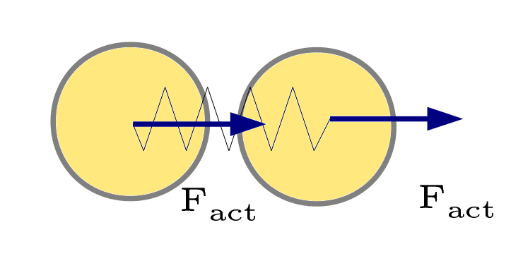
Figure 1: (Color online.) A sketch of an active dumbbell molecule.

The Péclet number, ${\rm Pe}$, is a dimensionless ratio between the advective transport rate and the diffusive transport rate. For particle flow one defines it as ${\rm Pe}=Lv/{D}$ , with $L$ a typical length, $v$ a typical velocity, and $D$ a typical diffusion constant in the problem. We choose $L\to\sigma_{\rm d}$, $v\to F_{\rm act}/\gamma$ and $D\to D^{\rm pd}_{\rm cm}=k_{B}T/(2\gamma)$ of the passive dumbbell [see Eq. (23)]; then,

$${\rm Pe}=\frac{2\sigma_{\rm d}F_{\rm act}}{k_{B}T}\;.$$ (13)

Another important parameter is the active Reynolds number

$${\rm Re}_{\rm act}=\frac{mF_{\rm act}}{\sigma_{\rm d}\gamma^{2}}\;,$$ (14)

defined in analogy with the usual hydrodynamic Reynolds number ${\rm Re}=Lv/\nu$, where $\nu$ is the kinematic viscosity of a given fluid, representing the ratio between inertial and viscous forces. Here we set $L\to\sigma_{\rm d}$, $v\to F_{\rm act}/\gamma$ and $\nu\to\gamma\sigma_{\rm d}^{2}/m_{\rm d}$.

III The molecular dynamics algorithm

We solved the stochastic Langevin equation with an algorithm due to Vanden-Eijinden and Ciccotti Vanden-Eijnden and Ciccotti (2006) that is exact to order $(\Delta t)^{2}$ with $\Delta t$ the time-step. We used a square bidimensional box with periodic boundary conditions.

The units of mass, length and energy are $m_{\rm d}$, $\sigma_{\rm d}$, and $\epsilon$, respectively. The adimensional elastic constant is defined as $k^{*}=k\sigma_{\rm d}^{2}/\epsilon$ and we take a large value $k^{*}=30$ to avoid the excessive extension of the dumbbell, and also prevent vibrations. The length $r_{0}$ in the FENE potential is rendered adimensional as $r_{0}^{*}=r_{0}/\sigma_{\rm d}$ and we used $r_{0}^{*}=1.5$. The thermal energy is normalized by the energy scale in the Lennard-Jones potential, $k_{B}T^{*}=k_{B}T/\epsilon$. The friction constant has dimensions of mass/time and we can make it adimensional as $\gamma_{\rm d}^{*}=\gamma/\sqrt{\epsilon m_{\rm d}/\sigma_{\rm d}^{2}}$. Physical realizations are usually in the over-damped regime which is ensured by choosing a value of $\gamma_{\rm d}^{*}$ such that ${\rm Re}_{\rm act}\ll 1$. We preferred to consider a model with inertial terms in order to have access to the crossover between ballistic and diffusive regimes. Concretely, we used $\gamma_{\rm d}^{*}=10$ for which the molecular oscillations are strongly inhibited. Finally, the adimensional temperatures $k_{B}T^{*}$ are in the range $0.001-1$. Once all parameters are expressed in terms of reduced units we can effectively set $m_{\rm d}=\sigma_{\rm d}=k_{B}=\epsilon=1$.

The optimal choice of time-step is delicate. We first identified some relevant time-scales in the problem and we later chose $\Delta t$. The time-scale for the oscillations of the free dumbbell is $\tau_{\rm osc}=2\pi\sqrt{m_{\rm d}/k}=2\pi/\sqrt{k^{*}}\sqrt{m_{\rm d}\sigma_{\rm d}^{2}/\epsilon}$ (and equals 1.14 for our choice of parameters). The inertial time scale is $t_{I}=m_{\rm d}/\gamma=1/\gamma_{d}^{*}\ \sqrt{m_{\rm d}\sigma_{\rm d}^{2}/\epsilon}$ (and equals 0.1 for our choice of parameters). We will show below that there is another time-scale, typically longer, associated to the angular diffusion, $t_{a}=\gamma R_{\infty}^{2}/(2k_{B}T)\approx\gamma_{\rm d}^{*}/(2k_{B}T^{*})\sqrt{m_{\rm d}\sigma_{\rm d}^{2}/\epsilon}$ where we used $R_{\infty}\approx\sigma_{\rm d}$ the typical length of the dumbbell molecule. We chose to work with $\Delta t=t_{I}/100$ to see details of the ballistic regime and $\Delta t=\tau_{\rm osc}/100$ to enter the later diffusive and active regimes. Times are measured in units of $\sqrt{(\sigma_{\rm d}^{2}m_{\rm d})/\epsilon}$.

IV Passive system

In this Section we review the behaviour of the passive dumbbell single molecule and interacting system, paying special attention to the dependence of the dynamic regimes on the surface fraction $\phi$.

IV.1 Passive single dumbbell

One can simply show that the equation of motion for the position of the center-of-mass, ${\mathbf{r}}_{\rm cm}=({\mathbf{r}}_{1}+{\mathbf{r}}_{2})/2$, of a single dumbbell governed by Eq. (5) under the same force ${\mathbf{f}}$ acting on each bead is

$$2m_{\rm d}\ddot{\mathbf{r}}_{\rm cm}(t)=-2\gamma\dot{\mathbf{r}}_{\rm cm}(t)+2{\mathbf{f}}(t)+{\bm{\xi}}(t)$$ (15)

with the new noise ${\bm{\xi}}(t)\equiv{\bm{\eta}}_{1}(t)+{\bm{\eta}}_{2}(t)$ with vanishing average, $\langle\xi_{a}(t)\rangle=0$, and correlation

$$\langle\xi_{a}(t)\xi_{b}(t^{\prime})\rangle=4\gamma k_{B}T\ \delta_{ab}\delta(t-t^{\prime})\;.$$ (16)

This is the Langevin equation of a point-like particle with mass $2m_{\rm d}$, under a force $2{\mathbf{f}}$ in contact with a bath with friction coefficient $2\gamma$ at temperature $T$. Equivalently, one can divide this equation by two and obtain a Langevin process for a point-like particle with mass $m_{\rm d}$ under a force ${\mathbf{f}}$ in contact with a bath with friction coefficient $\gamma$ at temperature $T/2$. From these analogies one recovers several results on the statistics of the center-of-mass position and velocity. Under no external force, ${\mathbf{f}}=0$, the center-of-mass velocity is distributed according to the Maxwell distribution for a particle with mass $2m_{\rm d}$ at equilibrium at temperature $T$ (or mass $m_{\rm d}$ at temperature $T/2$). The center-of-mass mean-square displacement between two times $t^{\prime}$ and $t$ after preparation

$$\Delta^{2}(t,t^{\prime})\equiv\langle[{\mathbf{r}}_{\rm cm}(t)-{\mathbf{r}}_{\rm cm}(t^{\prime})]^{2}\rangle$$ (17)

can be calculated as

$$\Delta^{2}(t,t^{\prime}) = d\Bigl{[}\Bigl{(}v_{0}^{2}-\frac{k_{B}T}{2m_{\rm d}}\Bigr{)}\frac{(e^{-\frac{\gamma}{m_{\rm d}}t^{\prime}}-e^{-\frac{\gamma}{m_{\rm d}}t})^{2}}{(\gamma/m_{\rm d})^{2}}$$ (18)

$$\;\;\;+\frac{k_{B}T}{\gamma}(t-t^{\prime})$$

$$\;\;\;-\frac{m_{\rm d}k_{B}T}{\gamma^{2}}(1-e^{-\frac{\gamma}{m_{\rm d}}(t-t^{\prime})})\Bigl{]}.$$

where $v_{0}$ is the velocity of the particle at the initial time $t=0$.

Given the inertial time

$$t_{I}=m_{\rm d}/\gamma\;,$$ (19)

one obtains different limits in relation to different values of $t$ and $t^{\prime}$. At short times $0\leq t^{\prime}\leq t\ll t_{I}$, by expanding all exponentials at small arguments, we obtain ballistic behaviour,

$$\Delta^{2}(t,t^{\prime})=dv_{0}^{2}\ (t-t^{\prime})^{2}\;.$$ (20)

At long total times $t\geq t^{\prime}\gg t_{I}$ and short time-delay $(t-t^{\prime})\ll t_{I}$, one also obtains ballistic behaviour,

$$\Delta^{2}(t,t^{\prime})=d\ \frac{k_{B}T}{2m_{\rm d}}\ (t-t^{\prime})^{2}\;,$$ (21)

with the initial velocity $v_{0}^{2}$ replaced by its average in equilibrium $\langle v^{2}\rangle=k_{B}T/(2m_{\rm d})$ (for a particle with mass $2m_{\rm d}$). In both cases the time-delay dependence crosses over to diffusive motion

$$\Delta^{2}(t,t^{\prime})=2dD^{\rm pm}_{\rm cm}\ (t-t^{\prime})\;,$$ (22)

for long time delay $(t-t^{\prime})\gg t_{I}$, with a diffusion constant taking the form

$$D^{\rm pd}_{\rm cm}=k_{B}T/(2\gamma)\;.$$ (23)

This is the diffusion constant used in the definition of the Péclet number in Eq. (13).

The length of the dumbbell molecule, ${\mathbf{R}}(t)={\mathbf{r}}_{1}-{\mathbf{r}}_{2}$, with ${\mathbf{r}}_{1}$ and ${\mathbf{r}}_{2}$ the position of the centers of the two spheres, is also a fluctuating quantity. For the parameters used one shows that $\langle R(t)\rangle$ approaches $R_{\infty}=0.96\approx\sigma_{\rm d}$. The angular degrees of freedom can also be simply analyzed, especially under the assumption that $R(t)$ is constant which is rather accurate since $R(t)$ does not fluctuate more than $3\%$ around its mean value. In this approximation one finds that the angle diffuses with an angular diffusion constant equal to

$$D_{a}=2k_{B}T/(\gamma R_{\infty}^{2})\;.$$ (24)

The linear instantaneous response, $R$, quantifies the effect of a small impulsive perturbation, say ${\mathbf{h}}(t^{\prime\prime})$ applied at time $t^{\prime\prime}$, on the dynamics of the system of interest. For a dumbbell moving in a plane, the $a$-th component of the center-of-mass position perturbed by a force acting on its $b$-th component, from time $t^{\prime}$ until time $t$, is

$$\langle r_{\rm cm}^{a}(t)\rangle_{\mathbf{h}}=\langle r_{\rm cm}^{a}(t^{\prime})\rangle+\int_{t^{\prime}}^{t}dt^{\prime\prime}\ R_{ab}(t,t^{\prime\prime})\ h_{b}(t^{\prime\prime})\;.$$ (25)

Equivalently,

$$R_{ab}(t,t^{\prime})\equiv\left.\frac{\delta\langle r_{\rm cm}^{a}(t)\rangle_{\mathbf{h}}}{\delta h_{b}(t^{\prime})}\right|_{{\mathbf{h}}=0}\;.$$ (26)

Motivated by the interpretation of Eq. (15) that keeps the temperature of the noise unaltered and equal to $T$, we take the perturbation to the center-of-mass to be ${\mathbf{h}}(t^{\prime\prime})=2{\mathbf{f}}(t^{\prime\prime})$. In order to focus on the long time limit of interest, $t\gg t_{I}$, and to simplify the expressions, we drop the inertia term from Eq. (15). In this limit, the center-of-mass position is given by

$${\mathbf{r}}_{\rm cm}(t)={\mathbf{r}}_{\rm cm}(t^{\prime})+\frac{1}{2\gamma}\int_{t^{\prime}}^{t}dt^{\prime\prime}\ [2{\mathbf{f}}(t^{\prime\prime})+{\bm{\xi}}(t^{\prime\prime})]\;.$$ (27)

The total linear response to a step-like perturbation that is applied from $t^{\prime}$ to $t$, with independent components $2f_{a}$ on each Cartesian spatial direction such that $\delta(2f_{a}(t^{\prime\prime}))/\delta(2f_{b}(t^{\prime}))=\delta_{ab}$, is then

$$\chi(t,t^{\prime})\equiv\int_{t^{\prime}}^{t}dt^{\prime\prime}\ R_{aa}(t,t^{\prime\prime})=\frac{d}{2\gamma}\ (t-t^{\prime})\;.$$ (28)

Summation over repeated indices was used to go from the second to third member of this equation. Comparing now to the mean-square displacement, $\Delta^{2}(t,t^{\prime})$, one finds that in the diffusive regime

$$2k_{B}T\chi(t,t^{\prime})=\Delta^{2}(t,t^{\prime})\;,$$ (29)

and both functions depend on the two times only through their difference, $t-t^{\prime}$. This relation is the same as the one for a point-like Brownian particle in contact with a bath at temperature $T$. We will use it as a reference to define the effective temperature from deviations in which the bath temperature is replaced by another parameter. (The comparison between $\chi$ and the time-derivative of the correlation function between the position measured at different times, which in equilibrium is proportional to the inverse temperature of the bath, yields a non-trivial relation that violates the equilibrium FDT for an unconfined Brownian particle L. F. Cugliandolo et al. (1994).)

A numerically convenient way to extract the linear response from Eq. (25), especially useful for the interacting systems studied in the following, consists in taking the perturbing forces ${\mathbf{f}}$ to be uncorrelated with the center-of-mass position and random, with zero mean, $[f_{a}]=0$, and correlation, $[f_{a}f_{b}]=f^{2}\delta_{ab}$. Multiplying Eq. (25) by $2f_{c}$ and taking the average over their distribution one finds

$$[\langle r_{\rm cm}^{a}(t)\rangle 2f_{c}]=(2f)^{2}\int_{t^{\prime}}^{t}dt^{\prime\prime}R_{ac}(t,t^{\prime\prime})\;.$$ (30)

Setting $a=c$ and summing over components one obtains

$$\chi(t,t^{\prime})=\frac{[\langle r_{\rm cm}^{a}(t)\rangle 2f_{a}]}{(2f)^{2}}\;.$$ (31)

Then, one derives from Eq. (27)

$$[\langle r_{\rm cm}^{a}(t)\rangle 2f_{a}]=\frac{1}{2\gamma}\ \delta_{aa}\ (2f)^{2}\ (t-t^{\prime})\;,$$ (32)

that yields

$$\chi(t,t^{\prime})=\frac{d}{2\gamma}(t-t^{\prime})$$ (33)

consistently with Eq. (28).

The way in which we probe the linear response of the interacting system is by applying a force of modulus $2f$ in a random direction to the center-of-mass, and not on the rotational and vibrational degrees of freedom, which gives a linear response proportional to $1/(2\gamma)$ in the case of a single passive dumbbell. Averaging over different angles, one recovers a result proportional to $1/(2\gamma)$. To obtain the linear response to independent perturbations applied on the spatial $d$ directions, that is to say $\chi$, we simply multiply the result by $d$.

IV.2 Passive many-body dumbbell system

In order to study the many-body system we performed numerical simulations in the form described in Sec. III. We averaged over 100 different realizations of a system with linear size $l=100$ and adimensional temperature $T=0.001$ (to make the notation lighter here and in what follows we avoid the asterisks to denote adimensional parameters). Measurements were done after an equilibration time of order $t_{\rm eq}=10^{2}$, starting from an initial random configuration of our system, in both the position of the center-of-mass and the angular direction of the dumbbells, and we show data gathered until a time equal to $10^{6}$.

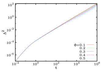
Figure 2: (Color online.) Mean-square displacement as a function of the delay time hereafter called $t$ measured after $t^{\prime}=100$, in a system of interacting passive dumbbells with the surface fractions given in the key at $T=0.001$ (double logarithmic scale).

First, we studied a very loose system, with $\phi=0.01$ (data not shown). From the analysis of the system’s global mean-square displacement we found that the ballistic regime ends at the inertial time $t_{I}=m_{\rm d}/\gamma\simeq 0.1$ when it crosses over to a diffusive regime. The ballistic regime is characterized by $\Delta^{2}(t)\simeq d\langle v^{2}\rangle t^{2}$ with $\langle v^{2}\rangle=k_{B}T/(2m_{\rm d})$ the thermal velocity of a Brownian particle with mass $2m_{\rm d}$, which for the parameters used takes the value $\langle v^{2}\rangle\simeq 5\cdot 10^{-4}$. The diffusion constant in the free-diffusive regime is very close to the one of the single passive dumbbell, $D_{\rm cm}\simeq D_{\rm cm}^{\rm pd}\simeq 5\cdot 10^{-5}$.

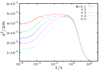
Figure 3: (Color online.) Rescaled mean-square displacement in systems of interacting passive dumbbells with the surface fractions given in the key. The data in Fig. 2 are divided by $2dt$ and presented as a function of $1/t$ to identify the diffusive regime as a plateau with height given by the diffusion constant. The single passive dumbbell diffusive constant takes the value $D_{\rm cm}^{\rm pd}=5\ 10^{-5}$ for these parameters, consistently with the trend of the numerical results for the many-particle system.

Next, we studied systems with five higher surface fractions: $\phi=0.1,\ 0.2,\ 0.3,\ 0.4,\ 0.5$, see Fig. 2. We found that, as in the single molecule case, the ballistic regime crosses over at $t_{I}=m_{\rm d}/\gamma=0.1$ to a first free diffusive regime, approximatively in the interval $1\leq t\lesssim 10^{2}$, that is now followed by a second diffusive regime that feels the effect of the dumbbell concentration Dhont (1996). Quite naturally, the dynamics slows down for denser systems as shown by the spread of curves at the late stages in the plot.

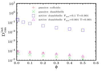
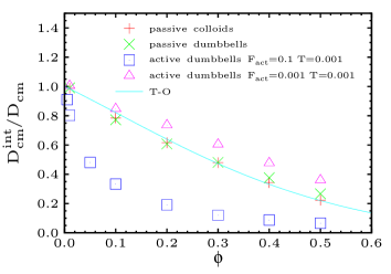
Figure 4: (Color online.) Upper panel: in linear-log scale, the diffusion constant of an interacting system, as a function of surface fraction $\phi$, in four cases: the passive dumbbell system displayed with (green) crosses $\times$; the passive colloidal system shown with (red) pluses $+$; the active dumbbell system with $F_{\rm act}=0.001$ and $F_{\rm act}=0.1$ drawn with (pink) triangles $\triangle$ and (blue) squares $\square$, respectively. In all cases the systems are in contact with the same thermal bath at temperature $T=0.001$ and interact with the same WCA potential given in Eq. (3). Lower panel: in double linear scale, the same data relative to its single particle limit, as a function of surface fraction $\phi$. The solid line represents the analytic prediction by Tokuyama-Oppenheim (TO) for a colloidal system with the same parameters Tokuyama and Oppenheim (1994).

In Fig. 3 data are represented in such a way that the last diffusive regime appears as a plateau at $1/t\to 0$ with height equal to the diffusive constant. The diffusive constant in the interacting regime, normalized by the one of the center-of-mass of the free passive dumbbell, $D_{\rm cm}^{\rm pd}$, is plotted in Fig. 4 against the surface fraction. For comparison we also similarly display normalised data obtained for a system of colloids coupled to the same thermal bath and interacting via the WCA potential (3). Within numerical accuracy the colloidal and dumbbell systems have the same behaviour until $\phi\lesssim 0.3$ while the dumbbell data are slightly above the colloidal ones for larger values of $\phi$. We find very good agreement with the prediction of Tokuyama and Oppenheim,

$$\frac{D_{\rm cm}(\phi)}{D_{\rm cm}(0)}=\frac{1}{1+H(\phi)}$$ (34)

with

$$H(\phi) = \frac{2[b(\phi)]^{2}}{1-b(\phi)}-\frac{c(\phi)}{1+2c(\phi)}$$ (35)

$$-\frac{b(\phi)\ c(\phi)\ [2+c(\phi)]}{[1+c(\phi)]\ [1-b(\phi)+c(\phi)]}$$

and

$$b(\phi)=\sqrt{9\phi/8}\qquad c(\phi)=11\phi/16\;,$$ (36)

derived from a perturbative calculation for low-concentrated colloidal systems Tokuyama and Oppenheim (1994). This expression has no free parameters. The agreement is very good for all surface fractions for colloids, and until $\phi\simeq 0.3$ for dumbbells (continuous line in the figure) if we use the three terms above in the expansion. For denser systems the shape of the molecules starts playing a role. We stress that the comparison is made between normalized curves. The third and fourth sets of data in this figure correspond to systems of active dumbbells and will be discussed in Sec. VI.

V Active single molecule

We turn now to the dynamics of a single active molecule as a reference case for the interacting system to be discussed in the next section.

Take a single active molecule constrained to move in two dimensional space. The length of the molecule is not altered by the active force and it still approaches $R_{\infty}\approx\sigma_{d}$. From the Langevin equation for the center-of-mass position that acquires a forcing term one calculates the average square velocity of the center-of-mass. For $t\gg t_{I}$ the stationary value for its $a$-th component is given by

$$\langle{v^{2}_{\rm cm}}_{a}(t)\rangle \to \frac{1}{2m_{\rm d}}\bigg{(}k_{B}T+\frac{F_{\rm act}^{2}}{\gamma(\frac{1}{t_{I}}+\frac{1}{t_{a}})}\bigg{)}$$ (37)

$$\equiv \frac{k_{B}T_{\rm kin}}{2m_{\rm d}}\;,$$

with the inertial and angular time-scales

$$t_{I}=\frac{m_{\rm d}}{\gamma}\;,\qquad\qquad t_{a}=\frac{1}{D_{a}}=\frac{\gamma\sigma_{\rm d}^{2}}{2k_{B}T}\;,$$ (38)

that will find a clear meaning when studying the mean-square displacement below.

The formula (37) gives an expression to what is called the kinetic or granular temperature Jaeger et al. (1996); Aranson and Tsimring (2006); Pouliquen and Forterre (2008) of the system. Quite naturally, $T_{\rm kin}=T$ for $F_{\rm act}=0$. Note that $T_{\rm kin}$ depends on the two time scales $t_{I}$ and $t_{a}$. It approaches

$$k_{B}T_{\rm kin} \simeq \left\{\begin{array}[]{ll}k_{B}T+t_{I}F_{\rm act}^{2}/\gamma&\mbox{for}\;\;\;\;\;\;\;\;t_{a}\gg t_{I}\;,\\ k_{B}T+t_{a}F_{\rm act}^{2}/\gamma&\mbox{for}\;\;\;\;\;\;\;\;t_{I}\gg t_{a}\;.\end{array}\right.$$ (40)

In our problem $t_{a}\gg t_{I}$ and the relevant limit is

$$k_{B}T_{\rm kin}=k_{B}T+\frac{m_{\rm d}}{\gamma^{2}}F_{\rm act}^{2}\;.$$ (41)

Moreover, for the parameter values later used in the simulation, $m_{\rm d}/\gamma^{2}=0.01$.

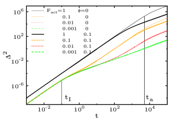
Figure 5: (Color online.) Mean-square displacement of active dumbbells for various values of $F_{\rm act}$ given in the key at temperature $T=0.001$ and linear size of the system $l=100$. The behaviour of a single dumbbell is shown with thinner lines while the one of a system of interacting dumbbells with $\phi=0.1$ is shown with thicker lines. The average has been taken over $200$ thermal histories. The inertial and angular time-scales are signaled with vertical black lines at $t_{I}=0.1$ and $t_{a}=5000$, respectively. The floating time-scale $t^{*}$ is proportional to the inverse square active force, $F_{\rm act}^{-2}$. See the text for a discussion of its effect.

After some simple calculations one finds that the mean-square displacement of a single dumbbell molecule moving on a plane under the longitudinal active force has an initial ballistic regime for times shorter than the inertial time-scale $t_{I}$. Beyond this time-scale, the over-damped limit takes over and inertia can be neglected. One can then quite easily derive the time-behaviour of the self-diffusion. For times shorter than the angular time scale $t_{a}$ one finds

$$\Delta^{2}(t)\simeq 2dD^{\rm pd}_{\rm cm}\ t+\left(\frac{F_{\rm act}}{\gamma}\right)^{2}t^{2}$$ (42)

with $D^{\rm pd}_{\rm cm}=k_{B}T/(2\gamma)$ the diffusion constant of the passive diatomic molecule (see also ten Hagen et al. (2011) where a similar calculation for an active ellipsoid has been performed). Within this regime one can still identify two sub-regimes. For times shorter than $t^{*}=2dD^{\rm pd}_{\rm cm}\gamma^{2}/F^{2}_{\rm act}$ the first term dominates and the dynamics is diffusive as in the absence of the active force. If, instead, times are longer than $t^{*}$ the dynamics becomes ballistic again and it is controlled by the active force. For even longer times, going beyond $t_{a}$, a new diffusive regime establishes,

$$\Delta^{2}(t)\simeq 2dD_{A}\ t\;,$$ (43)

with a diffusion constant that depends upon the active force and in $d=2$ is equal to

$$D_{A} = D^{\rm pd}_{\rm cm}+\frac{1}{2}\left(\frac{F_{\rm act}}{\gamma}\right)^{2}\frac{1}{D_{a}}.$$ (44)

In order to make the parameter dependence explicit we call this diffusion constant

$$\!\!\!\!D_{A}(F_{\rm act},\phi=0)\! = \!\frac{k_{B}T}{2\gamma}\!\left[1+\frac{1}{2}\!\left(\frac{F_{\rm act}\sigma_{\rm d}}{k_{B}T}\right)^{2}\right]$$ (45)

with $R_{\infty}$ replaced by $\sigma_{\rm d}$. This expression shows a dependence on the square of the Péclet number that will later appear in the effective temperature as well. The reason why the dynamics slow down in this last regime although there is still the active force acting on the dumbbell is that the angular motion goes against the translational one. All these regimes are summarized in

$$\mbox{ballistic}\mapsto\mbox{diffusive}\mapsto\mbox{ballistic}\mapsto\mbox{diffusive}$$

$$\qquad\;\;\;\;\;t_{I}\qquad\qquad\;\;t^{*}\qquad\;\;\;\;\;\;t_{a}$$

with the time-scales $t_{I}$ and $t_{a}$ introduced in Eq. (38). Note that the “intermediate” time-scale $t^{*}$ is inversely proportional to the square of the active force, $F^{-2}_{\rm act}$, and can go below the inertial time-scale $t_{I}$ for sufficiently strong non-equilibrium forcing or beyond $t_{a}$ for sufficiently weak one.

The generic features described in the previous paragraph can be seen in Fig. 5, especially in the curves for $F_{\rm act}=0.1,\ 0.01$, where $t^{*}<t_{a}$ and the regimes separated by $t^{*}$ are distinct. $t^{*}$ goes below $t_{I}$ for the largest active force $F_{\rm act}=1$ used in Fig. 5 for which the data shown have already reached the second ballistic regime and cross over, at $t_{a}$, to the last diffusive regime. At the other extreme, for the smallest active force $F_{\rm act}=0.001$ the time-scale $t^{*}$ is very large going beyond the time-scale $t_{a}$. The data show the first ballistic regime, the cross-over to the first free-diffusive regime and a very smooth cross-over to the last diffusive regime with a different diffusion constant. There is no second ballistic regime in this case. For the intermediate active forces, $F_{\rm act}=0.1,\ 0.01$, the four regimes can be observed in the data curves. The numerical results yield values for the cross-over times, diffusion constants and velocities in the ballistic regimes that are indistinguishable – within numerical accuracy – from the analytic predictions.

A similar crossover in the mean-square displacement was observed in systems and models of spherical particles. On the theoretical side, reference to such a crossover is made in Fily and Marchetti (2012); Levis and Berthier (2014); ten Hagen et al. (2011). In Howse et al. (2007) the dynamics of artificial swimmers made of polystyrene microspheres coated with platinum on one size, while keeping the second half as the non-conducting polystyrene, was studied. In this system, the platinum catalyzes the reduction of a ‘fuel’ of hydrogen peroxide to oxygen and water propelling the particles in a preferred direction. Particle tracking was used to characterise the particle motion as a function of hydrogen peroxide concentration. At short times, the particles move predominantly in a directed way, with a velocity that depends on the concentration of the fuel molecules, while at long times the motion randomises and becomes diffusive, with a diffusion constant that also depends on the fuel concentration. The analytic results for the single dumbbell mean-square displacement are consistent with the experimental results. A similar crossover was also observed in the motion of beads propelled by adsorbed bacteria Darnton et al. (2004) and in bacterial baths Wu and Libchaber (2000).

Another, independent probe of the dynamics of an out of equilibrium system is the displacement induced by applying a small constant external force to one (or more) tagged particle(s) in the system:

$$\chi(t) \equiv \frac{d}{N(2f)^{2}}\sum_{i=1}^{N}\langle 2{\mathbf{f}}_{i}\cdot{\mathbf{r}}_{{\rm cm}_{i}}(t)\rangle$$ (46)

$$= \frac{d}{N(2f)^{2}}\sum_{i=1,3,5,...2N}\langle 2{\mathbf{f}}_{i}\cdot\frac{{\mathbf{r}}_{i}(t)+{\mathbf{r}}_{i+1}(t)}{2}\rangle$$

$$= \frac{d}{N(2f)^{2}}\sum_{i=1}^{2N}\langle{\mathbf{f}}_{i}\cdot{\mathbf{r}}_{i}(t)\rangle\;.$$

This equation generalises (31) to the many-body system.

The perturbing force ${\mathbf{f}}_{i}={\bm{\epsilon}}_{i}f$ is applied to every monomer (in the same way as the active force) at time $t_{0}$ and kept constant until the measuring time $t$. $f$ is its modulus and ${\bm{\epsilon}}_{i}$ its direction which is uniformly distributed and is the same for the two monomers of a given dumbbell. In the case of a single active dumbbell $N=1$ and one finds again

$$\chi(t)=d(2\gamma)^{-1}\ t$$ (47)

a result that is independent of the activation force $F_{\rm act}$. We will write it as

$$\chi(t)=d\mu(F_{\rm act},\phi=0)\ t$$ (48)

with $\mu(F_{\rm act},\phi=0)=\mu(F_{\rm act}=0,\phi=0)$. Using the relation between mean-square displacement, $\Delta^{2}$, and induced displacement, $\chi$, in equilibrium, $2k_{B}T\chi(t)=\Delta^{2}(t)$ for all $t$, to define a possibly time-dependent effective temperature out of equilibrium

$$2k_{B}T_{\rm eff}(t)\chi(t)=\Delta^{2}(t)\;,$$ (49)

one finds, in the late diffusive regime $t\gg t_{a}$,

$$k_{B}T_{\rm eff}(t) \to k_{B}T_{\rm eff}(F_{\rm act},\phi=0)$$ (50)

$$= \frac{D_{A}(F_{\rm act},\phi=0)}{\mu(F_{\rm act},\phi=0)}$$

that becomes

$$T_{\rm eff}(F_{\rm act},\phi=0) = T\left[1+\frac{1}{2}\left(\frac{F_{\rm act}\sigma_{\rm d}}{k_{B}T}\right)^{2}\right]$$ (51)

$$= T\left(1+\frac{1}{8}\mbox{Pe}^{2}\right)\;.$$

We can arrive at the same result by defining $T_{\rm eff}$ from the Einstein relation between diffusion constant and mobility. We stress the fact that $T_{\rm eff}$ takes a constant value in this late diffusive regime. Note the different bath-temperature dependence in $T_{\rm eff}$ and $T_{\rm kin}$. We reckon also that $T_{\rm eff}\geq T_{\rm kin}$ and that the two expressions coincide in the (unphysical) case $t_{I}\gg t_{a}$. For the parameter values later used in the simulations $k_{B}T_{\rm eff}=k_{B}T+0.5\ F_{\rm act}^{2}/(k_{B}T)$ and the factor in the $F_{\rm act}^{2}$ term in $k_{B}T_{\rm eff}$ equals 10 at $T=0.05$ (while the one in $k_{B}T_{\rm kin}$ is only 0.01).

The response-displacement relation in a stochastic model for an active particle was studied in Ben-Isaac et al. (2011). In this paper, an overdamped Langevin equation for a randomly kicked point-like particle with a variable number of kicking motors producing pulses of force $\pm f_{0}$ acting at Poisson distributed times during intervals of duration $\Delta\tau$, and in contact with a thermal environment, was analyzed. In the low frequency limit (long time-delays) the effective temperature approaches a constant $T_{\rm eff}\to T+N_{m}f_{0}^{2}\Delta\tau^{2}/(\tau+\Delta\tau)$ with $N_{m}$ the number of motors and $\tau$ the averaged waiting-time between the pulses. The dependence on $f_{0}^{2}$ is similar to the dependence on Pe² that we find for the single active dumbbell.

Again from the $T_{\rm eff}$ perspective, Szamel Szamel (2014) studied a different model in which the self-propulsion of a single point-like active particle is modelled as a fluctuating force evolving according to the Ornstein-Uhlenbeck process, independently of the state of the particle. The particle moves in a viscous medium that is assumed to force overdamped motion. The free diffusion properties of the particle lead to an effective temperature defined from an extension of the Einstein relation linking the diffusion coefficient of the free particle to the variance of the fluctuating term in the Ornstein-Uhlenbeck process for the active force and the friction coefficient of the medium. The mobility and self-diffusion of an active Janus particle were monitored with micro-tracking by Palacci et al. Palacci et al. (2010) to infer from them the effective temperature. In both cases, as for our active single dumbbell, the effective temperature increases with the activation parameter as Pe².

Palacci et al. Palacci et al. (2010), Tailleur and Cates Tailleur and Cates (2008, 2009) and Szamel Szamel (2014) measured and calculated the stationary probability distribution of the active particles’ positions in a linear external potential (mimicking gravity) in a regime such that the sedimentation velocity is small with respect to the swimming velocity. They found an exponential form that corresponds to a Boltzmann distribution under gravity, with the parameter associated to the sedimentation length given by the equilibrium one with the temperature being replaced by the effective one of the free active particle. Szamel also studied whether the ambient temperature is simply replaced by the single particle effective one in the position probability distribution function of the Ornstein-Uhlenbeck active particle under a different external potential and found that this is not the case Szamel (2014).

VI Active many-body dumbbell system

The collective behavior of an ensemble of dumbbell molecules in interaction and under the effect of active forces is very rich Gonnella et al. (2013); Suma et al. (2014). In this section we first describe some general features of this behavior in the homogeneous phase. Later, we will focus on the evaluation of the diffusion constant, linear response and effective temperature.

VI.1 Homogeneous phase

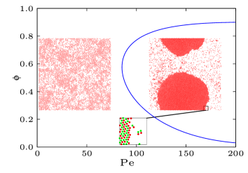
Figure 6: (Color online.) Schematic phase diagram of the dumbbell system. Inside the curve, at high Péclet numbers, the system undergoes phase separation into two phases characterized by two different densities. Here, typically, large and stable clusters are observed, as shown in the snapshot on the right. The dumbbells are freezed and point preferentially towards the center of the cluster. The enlargement shows the border of such a cluster, with the green part, corresponding to the head of the dumbbells, pointing inside, and the tails (red part) pointing outside. For small Péclet numbers the system does not show the formation of such large clusters and a typical configuration is presented. The location of the transition line is based on the results of simulations with $F_{\rm act}=1$ (see Gonnella et al. (2013); Suma et al. (2014) for further details); the right snapshot is taken at $T=0.01$, the one on the left at $T=0.05$.

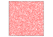
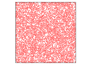
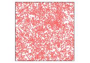
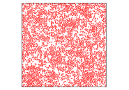
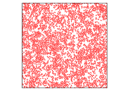
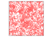
Figure 7: (Color online.) Clustering effects in the active many-body system. Density is $\phi=0.4$, temperature is $T=0.05$ and from left to right and top to bottom the active forces are $F_{\rm act}=0.01,\ 0.1,\ 0.3,\ 0.5,\ 0.7,\ 1$. The side of the box is $l=100$.

Active dumbbell systems exhibit a transition between a phase at small Péclet number, that includes the passive limit, and a phase with stable aggregates of dumbbells, not existing without activity, at high Péclet number. A schematic representation of the phase diagram is given in Fig. 6. We will not discuss the details of this phase diagram here but we simply state that we will work with sufficiently low Péclet number so as to stay in the region that we call the homogeneous phase although clustering phenomena, that will be important for the effective temperature, are already present. Typical configurations for the two phases are also shown in Fig. 6. In the aggregated phase the clusters reach the size of the system, while in the homogeneous phase they remain of finite size and are not stable. The phase separating kinetics in the phase with large-scale aggregation was studied in Gonnella et al. (2013). One can also observe that, while in the clusters of the homogeneous phase the dumbbells are not stucked and can move, they are frozen inside the aggregates in the high Péclet phase.

Figure 7 shows six typical snapshots of the system, all at the same density $\phi=0.4$ and temperature $T=0.05$ but for different active forces, $F_{\rm act}=0.01,\ 0.1,\ 0.3,\ 0.5,\ 0.7,\ 1$ (in reading order). The corresponding Péclet numbers vary in the interval $[0.4,40]$ which is well inside the homogenous phase in the phase diagram of Fig. 6. On the four last snapshots, i.e. beyond $F_{\rm act}\simeq 0.3$ we start seeing clustering effects. Their presence becomes less relevant moving away from the critical surface in parameter space. Configurations of the system for different densities at fixed active force strength are shown in Fig. 8.

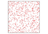
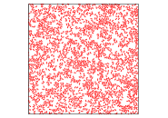
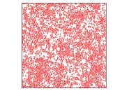
Figure 8: (Color online.) Clustering effects in the active many-body system. In all snapshots the active force strength is $F_{\rm act}=0.5$ and the temperature is $T=0.05$, while the densities are $\phi=0.1,\ 0.2,\ 0.3,\ 0.4$ (in reading order). The side of the box is $l=100$.

In Fig. 9 we show the static structure factor

$$S(q)=\frac{1}{N}\sum_{i=1}^{N}\langle|e^{i{\mathbf{q}}\cdot{\mathbf{r}}_{i}}|^{2}\rangle$$ (52)

of a system with $\phi=0.1$ (upper panel) and $\phi=0.4$ (lower panel) for different active forces, $F_{\rm act}=0.01,\ 0.1,\ 0.3,\ 0.5,\ 0.7,\ 1$ following the line code given in the keys. The positions ${\mathbf{r}}_{i}$ here are taken to be the ones of the two beads in the diatomic molecule. This function characterises the strength of density fluctuations at a length scale of the order of $2\pi/q$. Let us first discuss the data for $\phi=0.4$ (lower panel). For small active force strength, $F_{\rm act}=0.01$, the system is very close to a simple fluid made of diatomic molecules. Consequently, two peaks are visible in the curve. One represents the molecule elongation, i.e. the distance between the two beads in the dumbbell, and it is located at $q\simeq 6.21$ that corresponds to $\ell\simeq 1$. The other one signals the typical distance between beads belonging to different dumbbells and is located at $q\simeq 3.5$, that is to say $\ell\simeq 1.79$. For increasing values of the active force, clustering is favoured, and molecules in them tend to be closer to each other. Therefore, the first peak (at longer distances in real space) progressively disappears while the second one (for distances of the order of $\ell\simeq 1$) increases its weight. However, the most important new feature in the curves is the appearance and growth of the structure factor close to vanishing $q$. We note that the curves intercept at $q\simeq 2.26$ and that the curves move upwards with increasing $F_{\rm act}$ for $q$ smaller than this value. This increase quantifies the presence and growth of the clusters with increasing activity. The larger values of the structure factor at small $q$ observed for $F_{\rm act}\geq 0.3$ correspond to the clustering effects observed in this range of $F_{\rm act}$ in Fig. 7.

Similar features in the structure factor were observed experimentally in Theurkau et al. (2012) and numerically in Fily and Marchetti (2012); Levis and Berthier (2014); ten Hagen et al. (2011). In the dilute polymer melt active sample studied in Loi et al. (2011a) no such important increase of the low-$q$ structure factor was observed and the conclusion was that active forces were making the sample more compact but uniformly, with no clustering effects. The special $q$ values for the dumbbell system with packing fraction $\phi=0.1$ are: the molecular elongation peak is here located at $q\simeq 6.67$, the curves intercept at $q\simeq 1.48$ and the second peak at $F_{\rm act}=0.01$ is not really visible.

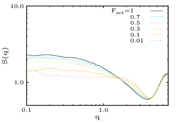
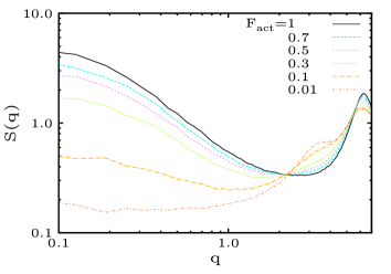
Figure 9: (Color online.) The structure factor of the active sample with $\phi=0.1$ (upper panel) and $\phi=0.4$ (lower panel) for different active force strengths given in the key. See the text for a discussion.

Although we have not shown it analytically, the probability distribution functions (pdf) of the velocity components is well represented by a Gaussian pdf with a kinetic temperature given by Eq. (37) for small values of $\phi$, as long as phase separation does not occur. These pdfs are shown with continuous and dashed lines in Fig. 10. Increasing the surface concentration, jamming effects slightly reduce the overall $T_{\rm kin}$.

In essentially out of equilibrium systems with non-potential forces that drive the dynamics, such as driven granular matter Jaeger et al. (1996); Aranson and Tsimring (2006); Pouliquen and Forterre (2008), vortex lattices Kolton et al. (2002) and the active matter we here study, the kinetic temperature should be higher than the ambient temperature. In our case we measured $T_{\rm kin}\simeq 0.05$ for $F_{\rm act}=0.01$ and $F_{\rm act}=0.1$, so that $T_{\rm kin}\simeq T$ in these two cases. For the strongest $F_{\rm act}$ used, $F_{\rm act}=1$, we measured $T_{\rm kin}=0.0596>T$. We can compare this value to the one expected for the single active dumbbell under the same conditions, according to Eq. (37): $T_{\rm kin}^{\rm single}\simeq 0.06$ which is very close to the value measured for the ensemble.

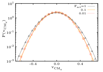
Figure 10: (Color online.) Pdf of the horizontal component of the center-of-mass dumbbell velocity, ${v_{CM}}_{x}$, in a system with $\phi=0.1$ at $T=0.05$, for three values of the active force, $F_{\rm act}=0.01,\ 0.1,\ 1$. Data are shown in linear-log scale. The values of the kinetic temperature, $T_{\rm kin}=0.0500,\ 0.0501,\ 0.0596$, respectively, used in the Gaussian fit shown with continuous and dashed lines are very close to the result for a single molecule, see Eq. (37). At $\phi=0.3$, for the same set of active forces, we have checked that the pdf is also well represented by a Gaussian distribution with $T_{\rm kin}$ given by Eq. (37).

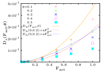
Figure 11: (Color online.) The diffusion constant in the active system at $T=0.05$, $D_{A}(F_{\rm act},\phi)$, as a function of $F_{\rm act}$ for five values of the system’s surface fraction given in the key. Normal scale is used. The continuous (orange) line is the analytic expression for $\phi=0$, see Eq. (45). The dashed (red) line is a fit of the data to the form $D_{A}(0,0.2)+aF_{\rm act}^{2}$ with $D_{A}(0,0.2)=0.00153$ obtained from the passive data at this temperature and $a=0.273$ (the $F^{2}_{\rm act}$ dependence found for the single molecule) for $\phi=0.2$ (green crosses $\times$). The dashed (blue) line is a fit to the form $D_{A}(0,0.2)+aF_{\rm act}^{\alpha}$ with $D_{A}(0,0.2)=0.00153$, $a=0.259$ and $\alpha\simeq 1.56$ (the fit used in Loi et al. (2008, 2011a), though $\alpha\simeq 2.3$ was found in that case for the low density used). The corrections to this fit will be studied in the next figures and discussed in the text.

VI.2 Mean-square displacement and asymptotic diffusion

VI.2.1 Very low temperature

In order to appreciate the effects of the dumbbell interaction, in Fig. 5 we showed with thicker lines the mean-square displacement in the active dumbbell system with $\phi=0.1$ and the same four values of the active force $F_{\rm act}=0.001,\ 0.01,\ 0.1,\ 1$ used in the single dumbbell case. Data for single and collective systems under the same active force are shown with the same color and line style. For the two smaller applied forces, $F_{\rm act}=0.001,\ 0.01$, we do not see any difference in $\Delta^{2}$ between the single and interacting case in this scale. For the two larger forces, $F_{\rm act}=0.1,\ 1$, the interaction between the molecules slows down the dynamics in the sense that the mean-square displacement of the interacting system, at the same time-lag, is smaller than the one for the single molecule. For the forces $F_{\rm act}=0.001,\ 0.01,\ 0.1$ we still see the angular time scale $t_{a}$, a feature that does not exist in models of point-like active particles as the ones studied in Loi et al. (2008, 2011a); Levis and Berthier (2014). Note that for $F_{\rm act}=1$ and such a low temperature, $T=0.001$, the system is in the phase-separated phase, the velocity-component pdf is no longer Gaussian (not shown) and the mean-square displacement is much slower than in the single molecule case.

A first presentation of the diffusion constant, $D_{A}(F_{\rm act},\phi)$ obtained by studying the system at the different surface fractions at a very low temperature, $T=0.001$, and for the active forces, $F_{\rm act}=0.1,0.001$, was given in Fig. 4. In this plot $D_{A}(F_{\rm act},\phi)$ was normalized by the center-of-mass diffusion constant of a single active molecule under the same conditions, $D_{A}(F_{\rm act},0)$. At $F_{\rm act}=0.1$, the data fall-off from 1 at $\phi=0$ very quickly as soon as $\phi>0$. At this very low temperature and relatively high active force small clusters appear and the diffusion properties are altered by them. On the other hand, at $F_{\rm act}=0.001$ the data are close to those for the passive system but they lie above them. They are not well represented by the TO expression and, moreover, they give a first indication of non-monotonic dependence of the normalised data with the active force, that we will discuss in more detail below when using a higher bath temperature.

VI.2.2 Working temperature

We will show in the following results for a higher temperature, $T=0.05$, such that, for all the active forces considered, the system is in the homogeneous phase, even though, as showed before, non–trivial fluctuation effects are clearly observable at sufficiently high values of $F_{\rm act}$. We also studied the system at other higher temperatures obtaining results similar to those found at $T=0.05$. (The values of the effective temperature found at $T=0.1$ will be reported in Table 1.)

The diffusion constant in the last diffusive regime of the active system is shown, as a function of active force, in Fig. 11 for five densities $\phi=0.1,\ 0.2,\ 0.3,\ 0.4,\ 0.5$. $D_{A}(F_{\rm act},\phi)$ was extracted from the analysis of the mean-square displacement in the late $t\gg t_{a}$ regime. The figure demonstrates that $D_{A}(F_{\rm act},\phi)$ decreases with increasing $\phi$ and increases with increasing $F_{\rm act}$. The analytic expression for the single particle limit, $\phi=0$, given in Eq. (45) is added with a continuous (orange) line. Clearly, the finite density induces a reduction of the diffusion constant for all $F_{\rm act}$. A quadratic fit of the data for $\phi=0.2$, which conserves the $F_{\rm act}^{2}$ dependence of the single particle limit, is shown with a dashed (red) line. More precisely, the form used is $D_{A}(0,0.2)+aF_{\rm act}^{2}$ with $D_{A}(0,0.2)=0.00153$ obtained from the passive data at this temperature and $a=0.273$ for $\phi=0.2$ (green crosses $\times$). Had we left the $F_{\rm act}=0$ intercept as a free parameter in this fit we would have obtained $0.0098$ which is relatively close to the actual passive limit, as it should. This fit is acceptable at small $F_{\rm act}$ but a deviation at large values of the active force is clear. Another fit, with an additional fit parameter as the power in the $F_{\rm act}$ dependence, is also shown with a dashed (blue) line. This fit was used in Loi et al. (2008, 2011b) to describe the diffusion constant of a rather dilute ensemble of interacting active point-like particles. We find here that a power law with $\alpha\simeq 1.56$ fits the dumbbell data at $\phi=0.2$ rather correctly for all $F_{\rm act}$ shown. The analysis of the $\phi$-dependence will be done next, where a more convenient way of describing these data will be proposed.

Figure 12: (Color online.) The diffusion constant, as extracted from the mean-square displacement of the dumbbells center-of-mass, as a function of $\phi$, in a system of active molecules at $T=0.05$. Upper panel: A linear-ln scale is used due to the large variation in the absolute values of $D_{A}(F_{\rm act},\phi)$. The values of $F_{\rm act}$ are given in the key. The values at $\phi=0$, shown with larger symbols, correspond to the theoretical value of $D_{A}$ for a single dumbbell given by Eq. (45). The data for relatively small $\phi$ are rather well fitted by a straight line, suggesting $\ln D_{A}(F_{\rm act},\phi)=\ln D_{A}(F_{\rm act},0)-b(F_{\rm act})\phi$ with $D_{A}(F_{\rm act},0)$ the single active molecule diffusion constant. In the lower panel the data are normalised by the diffusion constant of the single molecule and they are presented in linear scale. Non-monotonic behaviour with respect to $F_{\rm act}$ is observed suggesting that the fitting function $b(F_{\rm act})$ should be non-monotonic.

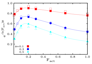
Figure 13: (Color online.) Upper panel: the exponential $e^{-b(F_{\rm act})\phi}$ for three densities given in the key. Original data are represented by open symbols while the filled symbols represent the values obtained from the fit in Eq. (53) of $\frac{D_{A}(F_{\rm act},\phi)}{D_{A}(F_{\rm act},0)}$ performed in Fig. 12. The lines are guides-to-the-eye obtained with a spline of the filled points. Lower panel: the correct TO description of data, $\frac{D_{A}(0,\phi)}{D_{A}(0,0)}=[1+H(\phi)]^{-1}$ for $F_{\rm act}=0$ (with red solid line), confronted to the exponential approximation in Eq. (53), that in this case yields $b(F_{\rm act}=0)=2.4$ (with green dashed line). The two curves are very close to each other up to $\phi\lesssim 0.3$.

In Fig. 12 we show the same diffusion constant, $D_{A}(F_{\rm act},\phi)$, as a function of the surface fraction $\phi$. The values of the active force $F_{\rm act}$ are given in the key. We have already stressed, when showing the very low temperature data, that as soon as $F_{\rm act}\neq 0$ the rather complex TO packing fraction dependence breaks down. We therefore seek for a different (and simpler) $\phi$-dependence of the diffusion constant of the active interacting sample. In the linear-ln presentation the data (up to $\phi\simeq 0.4$) are rather well fitted by a straight line, suggesting

$$D_{A}(F_{\rm act},\phi)\simeq D_{A}(F_{\rm act},0)\ e^{-b(F_{\rm act})\phi}$$ (53)

with $D_{A}(F_{\rm act},0)$ the single active molecule diffusion constant. (This is confirmed by a double linear presentation of data.) The exponential dependence on $\phi$ is much simpler than the TO expression and it cannot be taken as a formal proposal for the behavior of $D_{A}$ as we do not have an analytic justification for it. We simply stress here that it provides an acceptable description of data at this temperature.

In the second panel in Fig. 12 the finite $\phi$ diffusion constant is normalised by the single molecule one, in the form used in Fig. 4. The plot shows an unexpected non-monotonic behavior as a function of $F_{\rm act}$ suggesting that the effective $b(F_{\rm act})$ should be non-monotonic. It is interesting to observe that the diffusion constant ratio increases at small values of $F_{\rm act}$ starting to decrease when clustering effects become relevant for $F_{\rm act}\geq 0.3$.

In the upper panel in Fig. 13 we display the exponential factor $e^{-b(F_{\rm act})\phi}$. We use open symbols for the result of the ratio $D_{A}(F_{\rm act},\phi)/D_{A}(F_{\rm act},0)$ between numerical data, and filled symbols for the the fit of $D_{A}(F_{\rm act},\phi)/D_{A}(F_{\rm act},0)$, as a function of $F_{\rm act}$. Three values of $\phi$ were used and are given in the key. Extracting $b(F_{\rm act})$ from here one confirms the non-monotonic dependence with $F_{\rm act}$ with $b$ varying in the interval $[1,\ 2.7]$, circa. One observes that the fit proposed in Eq. (53) works reasonably well for all the values considered for $F_{\rm act}$. The approximate exponential fit of data is compared to the TO prediction for $F_{\rm act}=0$ in the lower panel. The two are very close for $\phi\lesssim 0.3$ while they deviate considerably for higher density.

To the best of our knowledge this non-monotonic behaviour has not been observed in the literature yet.

VI.3 The linear response function

We now turn to the study of the linear response function, integrated over a period of time, as defined in Eq. (46).

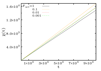
Figure 14: (Color online.) The induced displacement or linear susceptibility for a system of active dumbbells at $T=0.05$ and surface fractions $\phi=0.1$ (above) and $\phi=0.3$ (below). The different values of the active force used are given in the key. The magnitude of the applied field is $f=0.01$. One sees a non-monotonic dependence of $\mu(F_{\rm act},\phi)$ on $F_{\rm act}$, similarly to what we observed in $D_{A}(F_{\rm act},\phi)/D_{A}(F_{\rm act},0)$.

We started with an analysis of the amplitude of the applied perturbation, so as to determine the optimal value to be used for each set of parameters. Indeed, one has to use a small enough applied force to keep the response within the linear regime, but large enough to reduce the fluctuations. We found that $f=0.01$ yields the best results.

Figure 15: (Color online.) Upper panel: The asymptotic slope of the integrated linear response $\mu(F_{\rm act},\phi)$ as a function of $\phi$ for various active forces given in the key. The two curves are exponential fits to the data for $F_{\rm act}=0.01,\ 0.1$; the pre factor is $1/(2\gamma)=0.05$. Lower panel: the ratio $\mu(F_{\rm act},\phi)/\mu(F_{\rm act},0)$ is plotted as a function of $F_{\rm act}$ for the density values given in the key. The scale on the right side gives the values of $\mu(F_{\rm act},\phi)$. With open symbols, the ratios between numerical data; with filled symbols the result of the exponential fit of data. The curves are non-monotonic and the relative motility is enhanced for active forces of the order of $0.1\lesssim F_{\rm act}\lesssim 0.4$.

Figure 14 shows the time integrated linear response function $\chi(t)$ as a function of time $t$ for various active many-body systems at $T=0.05$ and $F_{\rm act}=0.001,\ 0.01,\ 0.1,\ 1$. In the two panels ($\phi=0.1$ and $\phi=0.3$) double linear scales are used and the dependence of the linear response integrated over time on $F_{\rm act}$ is now made visible. The induced displacement at a given time $t$ decreases with the dumbbells’ concentration. While the $F_{\rm act}=0.001$ and $F_{\rm act}=0.01$ curves lie on top of each other (within numerical accuracy), we notice the non-monotonic dependence on $F_{\rm act}$ for higher activities. Indeed, in both panels the curve for $F_{\rm act}=0.1$ lies above the ones for $F_{\rm act}=0.001,\ 0.01$ and $F_{\rm act}=1$. Moreover, the data for $F_{\rm act}=0.01$ and $F_{\rm act}=1$ appear in different order for $\phi=0.1$ and $\phi=0.3$. We have not included data for intermediate active forces $0.1<F_{\rm act}<1$ in this plot to ease the visualization but we have analysed them to extract the asymptotic slope (see the data presented in Fig. 15 below).

The non-monotonic dependence of $\chi(F_{\rm act},\phi)$ on $F_{\rm act}$ for sufficiently large $\phi$ is reminiscent of – though not the same as – a negative resistivity, that is to say a decreasing dependence of a current on the applied field that drives it, observed, for instance, in sufficiently dense kinetically constrained systems Sellitto (2008).

We extract the slope of these time-dependent curves for times such that $t\gg t_{a}$ and we call it $d\mu(F_{\rm act},\phi)$. We already know that at fixed $F_{\rm act}$, it is a decreasing function of the dumbbell concentration $\phi$, and that at fixed density it is a non-monotonic function of $F_{\rm act}$.

The study of the dependence of $\mu$ on these two parameters is performed in Fig. 15. In the upper panel we plot $\mu(F_{\rm act},\phi)$ as a function of $\phi$ for several active forces given in the key. We confirm the monotonic decay with increasing density. The two dashed curves are exponential fits as function of $\phi$ for two choices of the active force, $F_{\rm act}=0.01,\ 0.1$.

However, the dependence on $F_{\rm act}$ is less straightforward. The curves for different $F_{\rm act}$ cross. For instance, there is an inverting value of $\phi$, say $\phi^{*}$, so that $\mu(F_{\rm act}=1,\phi<\phi^{*})$ is smaller that $\mu(F_{\rm act}=0.1,\phi<\phi^{*})$ while one observes $\mu(F_{\rm act}=1,\phi>\phi^{*})>\mu(F_{\rm act}=0.1,\phi>\phi^{*})$. At fixed density, the relative motility is enhanced for active forces of the order of $0.1\lesssim F_{\rm act}\lesssim 0.4$ but the trend is reversed for higher active forces. The maximal effect is seen for $\phi\simeq 0.2$.

In the second panel we show the $F_{\rm act}$-dependence of the ratio $\mu(F_{\rm act},\phi)/\mu(F_{\rm act},0)$ for three packing fractions given in the key. The factor $\mu(F_{\rm act},0)=1/(2\gamma)$ is just a constant independent of $F_{\rm act}$ and $\phi$. We use open data points to represent the ratio between the numerical data, and filled symbols with joining lines to represent the outcome of the fit to an exponential:

$$\mu(F_{\rm act},\phi)=\mu(F_{\rm act},0)\ e^{-c(F_{\rm act})\ \phi}\;.$$ (54)

Note that if $c(F_{\rm act})$ were given by $b(F_{\rm act})$ as for the diffusion constant, we would have a $\phi$-independent $T_{\rm eff}$, and the same as for $\phi=0$. We obtain a non-monotonic dependence on $F_{\rm act}$ for $\phi\lesssim 0.4$ while the data for the highest density, $\phi=0.5$, may approach a plateau at the value reached at $F_{\rm act}=0.1$.

VI.4 Fluctuation-dissipation relation

In Fig. 16 we display the parametric plot $\Delta^{2}(\chi)$ for the three choices of activity, $F_{\rm act}=0.01,\ 0.1,\ 1$ and two surface fractions $\phi=0.1,\ 0.3$ all at $T=0.05$. We see a very weak dependence on $\phi$ and a strong dependence on $F_{\rm act}$. All data points at $F_{\rm act}=0$ (not shown) fall on top of each other (independently of $\phi$) as the passive system is in equilibrium with the bath. The data for $F_{\rm act}=0.01$ are very close to these and the data fit gives values of the effective temperature (the exponential of the vertical axis off-set of the slope of the curves) that are near the ambient temperature as well (see the numerical estimates in Table 1).

For larger values of the activity, the parametric construction displays the familiar shoulder separating short from long time-delay behaviour Cugliandolo et al. (1997); Cugliandolo (2011). The short time-delay fluctuations are much affected by the microscopic dynamics controlled, in this case, by the ambient temperature (the same for all sets of curves) and the activity (very different for the three sets of curves shown with different colour and line style).

After the shoulder, at long time-delays, the structural dynamics where interactions between dumbbells are important sets in. The effective temperature will be extracted from the slope of the parametric curves (in linear scale) in this time-delay regime, or from the vertical axis off-set of the slope in the late-time regime in double logarithmic scale, as explained above. That is to say, the asymptotic relation between linear integrated response and mean-square displacement allows one to extract the effective temperature as

$$k_{B}T_{\rm eff}(F_{\rm act},\phi)=\frac{D_{A}(F_{\rm act},\phi)}{\mu(F_{\rm act},\phi)}\;.$$ (55)

The effective temperature values are larger than the environmental temperature for $F_{\rm act}>0$. The numerical dependence of $T_{\rm eff}$ on $F_{\rm act}$ is reported in Fig. 17, where $T_{\rm eff}$ against $F_{\rm act}$ is shown. Note that $T_{\rm eff}$ is consistently larger than $T$ and increases with $F_{\rm act}$. The solid line in the plot represents the theoretical result for a single active dumbbell, $T_{\rm eff}\simeq T+cF_{\rm act}^{2}/T$. The quadratic dependence on $F_{\rm act}^{2}$ is similar to what was found for interacting active point-like particles Loi et al. (2008, 2011a) and interacting active polymers Loi et al. (2011b, a) at low density, comparable to $\phi\simeq 0.1$ in our case where no aggregation effects exist. The square power-law dependence on $F_{\rm act}$ also applies to the dumbbell data for $\phi=0.1$. Although in this double logarithmic scale the data seem to be very close to this form for all $\phi$, as we will see, a closer look at them shows a non-trivial $\phi$ dependence.

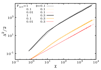
Figure 16: (Color online.) Parametric plot $\Delta^{2}(\chi)$ for three values of the activity, $F_{\rm act}=0.01,\ 0.1,\ 1$, two values of the surface concentration $\phi=0.1,\ 0.3$, and $T=0.05$. Double logarithmic representation. The effective temperature can be read from the off-set in the $y$ direction of the projection of the straight line in the long-time regime after the shoulder, $\ln T_{\rm eff}=\ln\Delta^{2}-\ln 2\chi$.

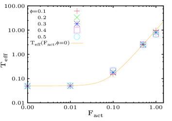
Figure 17: (Color online.) Fitted values of $T_{\rm eff}$ from the parametric plot in Fig. 16 for five values of $\phi$ given in the key, all at the temperature $T=0.05$. In this representation, all data seem to be in good agreement with the $T_{\rm eff}$ formula for a single dumbbell, Eq. (51), that is represented with the solid line. However, the actual values of $T_{\rm eff}$ are given in Table 1 where one sees that there is, though, a weak difference in the data for different $\phi$: for $F_{\rm act}=0.1$, $T_{\rm eff}$ tends to increase with increasing $\phi$, while for $F_{\rm act}=1$, $T_{\rm eff}$ tends to decrease with increasing $\phi$.

The results for $T_{\rm eff}$ for two working temperatures, $T=0.05$ and $T=0.1$, are summarised in Table 1. At very small active force we find $T_{\rm eff}\simeq T$ at all densities, as expected as the system is near equilibrium (see the first rows in the two sets of data shown in Table 1). For intermediate active forces, e.g. $F_{\rm act}=0.1$ (third rows in the tables), we see that $T_{\rm eff}$ is significantly larger than $T$ and that it weakly increases with increasing $\phi$. For still larger active forces the dependence on $\phi$ changes, as $T_{\rm eff}$ decreases with $\phi$ for sufficiently large values of $\phi$ ($\phi\stackrel{{\scriptstyle>}}{{\sim}}0.1$ for $T=0.05$ and $\phi\stackrel{{\scriptstyle>}}{{\sim}}0.3$ for $T=0.1$, when $F_{\rm act}=1$). Consistently with what discussed in the previous paragraph, for fixed density, $T_{\rm eff}$ increases with $F_{\rm act}$ for the two working temperatures. Moreover, at fixed density and active force $F_{\rm act}>0.5$ we see that $T_{\rm eff}$ is lower at higher temperature.

$T=0.05$
$F_{\rm act}\$	$\ \phi=0\$	$\ \phi=0.1\$	$\ \phi=0.3\$	$\ \phi=0.5\$
0.001	0.0500	0.0499	0.0488	0.0502
0.01	0.0509	0.0498	0.0502	0.0522
0.1	0.142	0.152	0.179	0.223
0.5	2.35	2.51	2.59	2.44
1	9.27	9.68	7.83	6.56

$T=0.1$
$F_{\rm act}\$	$\ \phi=0\$	$\ \phi=0.1\$	$\ \phi=0.3\$	$\ \phi=0.5\$
0.001	0.100	0.102	0.100	0.097
0.01	0.100	0.100	0.100	0.101
0.1	0.146	0.158	0.167	0.201
0.5	1.25	1.34	1.56	1.77
1	4.71	5.03	5.10	4.92

Table 1: Values of $T_{\rm eff}$ from the analysis at different active forces and system’s densities, at $T=0.05$ and $T=0.1$.

In Fig. 18 we display the ratio between the finite density effective temperature and the single molecule limit one as a function of the strength of the active force, $T_{\rm eff}(F_{\rm act},\phi)/T_{\rm eff}(F_{\rm act},0)$ vs. $F_{\rm act}$. If we could separate the diffusion coefficient of a single dumbbell from the $\phi$ dependence as proposed in Eq. (53), and if we had the same density dependence of the $\mu(F_{\rm act},\phi)$ as in the remaining factor in $D_{A}(F_{\rm act},\phi)$, meaning $b(F_{act})=c(F_{act})$, then $T_{\rm eff}(F_{\rm act},\phi)$ should be independent of $\phi$ and just equal to $T_{\rm eff}(F_{\rm act},0)$. The data show that this holds for $\phi=0.1$ where the data points are (within numerical accuracy) constant but it does not for higher densities. For $\phi\geq 0.1$ one observes a non–monotonic dependence of $T_{\rm eff}(F_{\rm act},\phi)/T_{\rm eff}(F_{\rm act},0)$ on $F_{\rm act}$, reflecting in some way the non–monotonic behavior first shown for the diffusion and response ratios $D_{A}(F_{\rm act},\phi)/D_{A}(F_{\rm act},0)$ and $\mu(F_{\rm act},\phi)/\mu(F_{\rm act},0)$. The finite density effective temperature is higher than the single molecule one for active forces in the interval $[0,0.5]$ while it is lower than the single molecule one for active forces in the interval $[0.5,1]$. A maximum is reached at around $F_{\rm act}\simeq 0.1$. We ascribe the change in behaviour to the presence of finite size clusters in the sample for $F_{\rm act}\stackrel{{\scriptstyle>}}{{\sim}}0.5$ and sufficiently large density. These clusters (see the last panels in Fig. 7) would respond differently from the homogeneous bulk and their dynamics will be different. We also note that these curves seem to cross at the active force strength value $F_{\rm act}=0.5$. A similar analysis of this ratio at a different temperature, $T=0.1$, shows that the crossing occurs at a different value of the active force strength, $F_{\rm act}\simeq 1$, that corresponds to the same Péclet number $\rm{Pe}=20$ (within numerical accuracy).

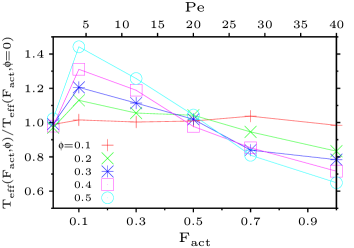
Figure 18: (Color online.) The ratio between the finite density effective temperature and the single molecule limit one as a function of the strength of the active force, $T_{\rm eff}(F_{\rm act},\phi)/T_{\rm eff}(F_{\rm act},0)$, where $T_{\rm eff}(F_{\rm act},0)=T\ [1+\mbox{Pe}^{2}/8]$. The temperature is $T=0.05$. See the text for a discussion.

Finally, we note that $T_{\rm eff}>T_{\rm kin}$ as soon as the active force is intense enough to see a considerable deviation of both from the ambient temperature. Confront, for instance, the analytic values $T_{\rm eff}=0.142$ and $T_{\rm kin}\simeq 0.050$ at $\phi=0$ and $F_{\rm act}=0.1$, and the numeric values $T_{\rm eff}\simeq 9.68$ and $T_{\rm kin}\simeq 0.06$ at $\phi=0.1$ and $F_{\rm act}=1$.

VII Conclusions

In this paper we studied the dynamic properties of isolated and interacting, passive and active, dumbbell systems.

The model studied here differs from other models of active matter previously studied in the literature with numerical techniques from a similar viewpoint. For instance, we do not impose polar alignment mechanisms as in Szabó et al. (2006); Henkes et al. (2011). The active forces used here are different from the ones used in the analysis of active macromolecules presented in Loi et al. (2011b, a): while in the dumbbell system the active forces act along the main axis of the molecule, in the polymer system the active forces act only on the center monomer and in random directions. The Langevin dynamics used in this paper is different from the Monte Carlo rule chosen in Levis and Berthier (2014) and from the run-and-tumble bacteria models in Tailleur and Cates (2008, 2009). Moreover, we did not distinguish translation and rotational noise, as done in Fily and Marchetti (2012), but we simply added independent Gaussian white noise (related to the friction dissipative term in the usual way) to the Langevin equations for the positions of the two atoms in the dumbbell.

For fixed temperature and active force strength, this very simple model has a phase transition between a homogeneous and a phase separated phase Gonnella et al. (2013); Suma et al. (2014). In this paper we focused on the low density phase in which the system is homogeneous on average with, possibly, giant density fluctuations for sufficiently high density Suma et al. (2014). We studied the dynamics for three different temperatures and a wide range of densities and active forces in this phase.

We first presented a detailed study of the mean-square displacement of the interacting active sample. We analysed the single passive and active dumbbell dynamics and we investigated how the finite density affects the various dynamic regimes and, in particular, the diffusive properties in the late time-delay limit that goes beyond the angular diffusion time of the single molecule. As one had expected, we found that the diffusion constant decreases with increasing density and increases with increasing active force. The ratio between the finite-density and the single particle diffusion constant exhibits an intriguing non-monotonic dependence on the active force. We also analysed how the Tokuyama-Oppenheim density-dependence expression for this ratio Tokuyama and Oppenheim (1994) is modified by self-propulsion, finding that a simpler exponential decay (with a non-monotonic active force dependent factor in the exponential) fits the data reasonably well.

We then studied the linear response function of the dumbbell displacement to infinitesimal perturbations that push them in random directions. As usual, to minimise the numerical error, we focused on the linear response integrated over time (instead of the instantaneous response that fluctuates much more). We found that, at fixed time delay, the integrated linear response decreases monotonically with increasing density. The dependence on the active force is again non-trivial, with a maximum response reached for active forces with strength in $0.1\lesssim F_{\rm act}\lesssim 0.3$ for densities in $0.1\lesssim\phi\lesssim 0.3$.

The kinetic temperature is extracted from the asymptotic value of a one-time observable, the kinetic energy. As already discussed in detail in the context of glassy systems and granular matter Cugliandolo et al. (1997); Cugliandolo (2011), although one proves that a system is not in equilibrium with the thermal bath whenever $T_{\rm kin}\neq T$, the reverse is not true. In glassy systems in relaxation $T_{\rm kin}=T$ while these systems evolve out of equilibrium. The reason is that the kinetic temperature carries information about a fast observable, the kinetic energy, that can be able to quickly equilibrate with the environment, while other observables, being slower, can still be far from equilibrium. Indeed, the kinetic temperature does not characterise the large scale structural relaxation of glassy or driven systems.

The effective temperature notion, as obtained from the deviation from the equilibrium fluctuation-dissipation theorem linking spontaneous and induced fluctuations, has proven to be very useful to understand the dynamics of slowly relaxing passive systems, such as glasses and gently sheared super-cooled liquids Cugliandolo (2011). This concept has been explored in some active systems as well as we explained in the introduction. In this work we studied the fluctuation-dissipation ratio for the low-density active dumbbell system and we characterised it as a function of density and activity. The effective temperature is always higher than the ambient temperature, it increases with increasing activity and, for small active force it monotonically increases with density while for sufficiently high activity it first increases to next decrease with the packing fraction. This effect should be due to the existence of finite-size clusters for sufficiently high activity and density at the fixed (low) temperatures at which we worked. The crossover occurs at lower activity or density the lower the external temperature. The finite density effective temperature is higher (lower) than the single dumbbell one below (above) a cross-over value of the Péclet number.

In the active dumbbell system we measured $T_{\rm kin}$ values that are very close to $T$ for $F_{\rm act}=0.01,\ 0.1,\ 1$. The existence of the kinetic temperature characterising the short-time delay behaviour of fluctuations, and the effective temperature extracted from the fluctuation-dissipation relations at long time-delays, does not invalidate the possible thermodynamic interpretation of the latter. One simply has to focus on the dynamics of the systems in one or another dynamic regime Cugliandolo et al. (1997); Cugliandolo (2011) and test its thermodynamic properties within in it.

We want to stress once again that the effective temperature is not a parameter that characterises the statistical properties of the activity but an intensive parameter that tells us about the dynamic properties of the interacting and active many-body system.

Fily and Marchetti Fily and Marchetti (2012) argue that the effective tempeature notion cannot apply to active matter systems in their dense phase. They base their claim on the comparison of instantaneous snapshots of typical clustered configurations and equivalent thermal equilibrium ones with similar overlap between particles at the same packing fraction. This argument cannot be used to refute the effective temperature ideas in this context (nor in the glassy context either) as its very definition is dynamic and correlation and linear response functions at different times need to be calculated to derive $T_{\rm eff}$. Having said this, the analysis of $T_{\rm eff}$ in a dense active phase has not been performed yet and we cannot claim that the concept will still be valid in this clustered phase.

The dumbbell system is particularly interesting as it allows one to study translational and, simultaneously, also rotational degrees of freedom. A recent analysis of the effective temperature ideas in a passive dumbbell system has shown that the relation between the two can depend non-trivially on the elongation of the molecule Ninarello et al. (2014). It would be very interesting to explore the effect of this parameter in the results that we showed and to investigate the fluctuation-dissipation relations of rotational degrees of freedom in the active dumbbell system as well.

The values of the effective temperatures found from the fluctuation-dissipation relation of the active system should be confirmed with alternative measurements to test their thermodynamic meaning. For instance, one could use spherical passive particles as tracers and measure the effective temperature from their diffusion properties (as in Wu and Libchaber (2000)) and kinetic energy fluctuations. We will report on the use of tracers in this context in a separate publication.

Finally, it would be interesting to analyse the effect that external potentials may have on the dynamics of this active dumbbell system. Tailleur and Cates derived a diffusive approximation for active run-and-tumble particles Tailleur and Cates (2008, 2009) and found that, for weak external potentials that modify only slightly the velocity of the particles, the system should follow equilibrium dynamics with the equilibrium bath temperature replaced by $T_{\rm eff}$. It will be interesting to check whether this result holds for the active dumbbell system under appropriate external forces and how it is modified by the finite density and interactions within the sample, and strong external potential forces.

Acknowledgments: We thank D. Loi and S. Mossa for very useful discussions. We warmly thank J. Tailleur for very useful comments on the manuscript. LFC is a member of Institut Universitaire de France. GG acknowledges the support of MIUR (project PRIN 2012NNRKAF).

References

- Toner et al. (2005) J. Toner, Y. Tu, and S. Ramaswamy, Ann. of Phys. 318, 170 (2005).
- Fletcher and Geissler (2009) D. A. Fletcher and P. L. Geissler, Ann. Rev. Phys. Chem. 60, 469 (2009).
- Menon (2010) G. I. Menon, Rheology of Complex Fluids p. 193 (2010).
- Ramaswamy (2010) S. Ramaswamy, Ann. Rev. Cond. Matt. Phys. 1, 323 (2010).
- Cates (2012) M. E. Cates, Rep. Prog. Phys. 75, 042601 (2012).
- Vicsek and Zafeiris (2012) T. Vicsek and A. Zafeiris, Phys. Rep. 517, 71 (2012).
- Marchetti et al. (2013) M. C. Marchetti, J. F. Joanny, S. Ramaswamy, T. B. Liverpool, J. Prost, M. Rao, and R. A. Simha, Rev. Mod. Phys. 85, 1143 (2013).
- Schwarz and Safran (2013) U. S. Schwarz and S. A. Safran, Rev. Mod. Phys. 85, 1327 (2013).
- de Magistris and Marenduzzo (2014) G. de Magistris and D. Marenduzzo, to appear in Physica A (2014).
- Narayan et al. (2007) V. Narayan, S. Ramaswamy, and N. Menon, Science 317, 105 (2007).
- Deseigne et al. (2010) J. Deseigne, O. Dauchot, and H. Chaté, Phys. Rev. Lett. 105, 098001 (2010).
- Paxton et al. (2004) W. F. Paxton, K. C. Kistler, C. C. Olmeda, A. Sen, S. K. S. Angelo, Y. Cao, T. E. Mallouk, P. E. Lammert, and V. H. Crespi, J. Am. Chem. Soc. 126, 13424 (2004).
- Hong et al. (2006) L. Hong, S. Jiang, and S. Granick, Langmuir 22, 9495 (2006).
- Palacci et al. (2010) J. Palacci, C. Cottin-Bizonne, C. Ybert, and L. Bocquet, Phys. Rev. Lett. 105, 088304 (2010).
- Romanczuk et al. (2012) P. Romanczuk, M. Bär, W. Ebeling, B. Lindner, and L. Schimansky-Geier, Eur. Phys. J. Special topics 202, 1 (2012).
- Czirók et al. (1997) A. Czirók, H. E. Stanley, and T. Vicsek, J. Phys. A 30, 1375 (1997).
- Vicsek et al. (1995) T. Vicsek, A. Czirók, E. Ben-Jacob, I. Cohen, and O. Shochet, Phys. Rev. Lett. 75, 1226 (1995).
- Tailleur and Cates (2008) J. Tailleur and M. E. Cates, Phys. Rev. Lett. 100, 218103 (2008).
- Fily and Marchetti (2012) Y. Fily and M. C. Marchetti, Phys. Rev. Lett. 108, 235702 (2012).
- Fily et al. (2014) Y. Fily, S. Henkes, and M. C. Marchetti, Soft Matter 10, 2132 (2014).
- Redner et al. (2013) G. S. Redner, M. F. Hagan, and A. Baskaran, Phys. Rev. Lett. 110, 055701 (2013).
- Buttinoni et al. (2013) I. Buttinoni, J. Bialké, F. Kümmel, H. Löwen, C. Bechinger, and T. Speck, Phys. Rev. Lett. 110, 238301 (2013).
- Stenhammar et al. (2013) J. Stenhammar, A. Tiribocchi, R. Allen, D. Marenduzzo, and M. Cates, Phys. Rev. Lett. 111, 145702 (2013).
- Gonnella et al. (2013) G. Gonnella, A. Lamura, and A. Suma, Int. J. Mod. Phys. C (2013).
- Suma et al. (2014) A. Suma, D. Marenduzzo, G. Gonnella, and E. Orlandini, submitted to EPL (2014).
- Levis and Berthier (2014) D. Levis and L. Berthier, Phys. Rev. E 89, 062301 (2014).
- Wittkowski et al. (2014) R. Wittkowski, A. Tiribocchi, J. Stenhammar, R. Allen, D. Marenduzzo, and M. Cates, Nat. Comm. 5, 4351 (2014).
- Ramaswamy et al. (2003) S. Ramaswamy, R. A. Simha, and J. Toner, Europh. Lett. 62, 196 (2003).
- Ginelli et al. (2010) F. Ginelli, F. Peruani, M. Bär, and H. Chaté, Phys. Rev. Lett. 104, 184502 (2010).
- Elgeti and Gompper (2009) J. Elgeti and G. Gompper, EPL 85, 38002 (2009).
- Elgeti and Gompper (2013) J. Elgeti and G. Gompper, EPL 101, 48003 (2013).
- Bricard et al. (2013) A. Bricard, J.-B. Caussin, N. Desreumaux, O. Dauchot, and D. Bartolo, Nature 503, 95 (2013).
- Wang and Wolynes (2011a) S. Wang and P. G. Wolynes, Proc. Nac. Acad. Sc. USA 108, 15184 (2011a).
- Shen and Wolynes (2004) T. Shen and P. G. Wolynes, Proc. Nac. Acad. Sc. USA 101, 8547 (2004).
- Angelini et al. (2011) T. E. Angelini, E. Hannezo, X. Trepat, M. Marquez, J. J. Fredberg, and D. A. Weitz, Proc. Nat. Acad. Sc. USA 108, 4714 (2011).
- Henkes et al. (2011) S. Henkes, Y. Fily, and M. C. Marchetti, Phys. Rev. E 84, 040301 (R) (2011).
- Berthier and Kurchan (2013) L. Berthier and J. Kurchan, Nature Phys. 9, 310 (2013).
- Chaté et al. (2006) H. Chaté, F. Ginelli, and R. Montagne, Phys. Rev. Lett. 96, 180602 (2006).
- Cates et al. (2008) M. E. Cates, S. M. Fielding, D. Marenduzzo, E. Orlandini, and J. M. Yeomans, Phys. Rev. Lett. 101, 068102 (2008).
- Saracco et al. (2009) G. P. Saracco, G. Gonnella, D. Marenduzzo, and E. Orlandini, Phys. Rev. E 80, 051126 (2009).
- Bees and Croze (2010) M. A. Bees and O. A. Croze, Proc. Roy. Soc. A: Math. Phys. and Eng. Sci. 466, 2057 (2010).
- Bearon et al. (2012) R. N. Bearon, M. A. Bees, and O. A. Croze, Phys. Fluids 24, 121902 (2012).
- Saracco et al. (2012) G. P. Saracco, G. Gonnella, D. Marenduzzo, and E. Orlandini, Central European Journal of Physics 10, 1109 (2012).
- Cugliandolo et al. (1997) L. F. Cugliandolo, J. Kurchan, and L. Peliti, Phys. Rev. E 55, 3898 (1997).
- Cugliandolo (2011) L. F. Cugliandolo, J. Phys. A: Math. and Theor. 44, 483001 (2011).
- Wu and Libchaber (2000) X.-L. Wu and A. Libchaber, Phys. Rev. Lett. 84, 3017 (2000).
- Shen and Wolynes (2005) T. Shen and P. G. Wolynes, Phys. Rev. E 72, 041927 (2005).
- Wang and Wolynes (2011b) S. Wang and P. G. Wolynes, J. Chem. Phys. 135, 051101 (2011b).
- Martin et al. (2001) P. Martin, A. J. Hudspeth, and F. Jülicher, Proc. Nac. Acad. Sc. USA 98, 14380 (2001).
- Mizuno et al. (2007) D. Mizuno, C. Tardin, C. F. Schmidt, and F. C. MacKintosh, Science 315, 370 (2007).
- Ben-Isaac et al. (2011) E. Ben-Isaac, Y.-K. Park, G. Popescu, F. L. Brown, N. S. Gov, and Y. Shokef, Phys. Rev. Lett. 106, 238103 (2011).
- Bohec et al. (2013) P. Bohec, F. Gallet, C. Maes, S. Safaverdi, P. Visco, and F. van Wijland, EPL 102, 50005 (2013).
- Fodor et al. (2014) E. Fodor, M. Guo, N. S. Gov, P. Visco, D. A. Weitz, and F. van Wijland (2014).
- Tailleur and Cates (2009) J. Tailleur and M. E. Cates, EPL 86, 60002 (2009).
- Szamel (2014) G. Szamel, Phys. Rev. E 90, 012111 (2014).
- Loi et al. (2008) D. Loi, S. Mossa, and L. F. Cugliandolo, Phys. Rev. E 77, 051111 (2008).
- Loi et al. (2011a) D. Loi, S. Mossa, and L. F. Cugliandolo, Soft Matter 7, 10193 (2011a).
- Loi et al. (2011b) D. Loi, S. Mossa, and L. F. Cugliandolo, Soft Matter 7, 3726 (2011b).
- Peruani et al. (2006) F. Peruani, A. Deutsch, and M. Bär, Phys. Rev. E 74, 030904(R) (2006).
- Yang et al. (2010) Y. Yang, V. Marceau, and G. Gompper, Phys. Rev. E 82, 031904 (2010).
- Peruani et al. (2012) F. Peruani, J. Starruss, V. Jakovljevic, L. Sogaard-Andersen, A. Deutsch, and M. Bär, Phys. Rev. Lett. 108, 098102 (2012).
- McCandlish et al. (2012) S. R. McCandlish, A. Baskaran, and M. F. Hagan, Soft Matter 8, 2527 (2012).
- Wensink et al. (2012) H. H. Wensink, J. Dunkel, S. Heindereich, K. Drescher, R. Goldstein, H. Lowen, and J. Yeomans, Proc. Nat. Acad. Sc. USA 109, 14308 (2012).
- Wensink et al. (2013) H. H. Wensink, H. Lowen, M. Marechal, A. Hartel, R. Wittkowski, U. Zimmermann, A. Kaiser, and A. M. Menzel, Eur. Phys. J. - Sp. Topics 222, 3023 (2013).
- Vásquez-Quesada et al. (2009) A. Vásquez-Quesada, M. Ellero, and P. Español, Phys. Rev. E 79, 056707 (2009).
- Kowalik and Winkler (2013) B. Kowalik and R. Winkler, J. Chem. Phys. 138, 104903 (2013).
- Alexander and Yeomans (2008) G. Alexander and J. Yeomans, Europh. Lett. 83, 34006 (2008).
- Putz et al. (2010) V. B. Putz, J. Dunkel, and J. Yeomans, Chemical Physics 375, 557 (2010).
- Gyrya et al. (2010) V. Gyrya, I. S. Aranson, L. Berlyand, and D. Karpeev, Bull. Math Biol. Chem. Phys. 72, 148 (2010).
- Valeriani et al. (2011) C. Valeriani, M. Li, J. Novosel, J. Arlt, and D. Marenduzzo, Soft Matter 7, 5228 (2011).
- Weeks et al. (1971) J. D. Weeks, D. Chandler, and H. C. Andersen, J. Chem. Phys. 54, 5237 (1971).
- Vanden-Eijnden and Ciccotti (2006) E. Vanden-Eijnden and G. Ciccotti, Chem. Phys. Lett. 429, 310 (2006).
- L. F. Cugliandolo et al. (1994) L. F. Cugliandolo, J. Kurchan, and G. Parisi, J. Phys. I (France) 4, 1641 (1994).
- Dhont (1996) J. K. Dhont, An introduction to dynamics of colloids, vol. 2 (Elsevier Science, 1996).
- Tokuyama and Oppenheim (1994) M. Tokuyama and I. Oppenheim, Phys. Rev. E 50, 16 (1994).
- Jaeger et al. (1996) H. M. Jaeger, S. R. Nagel, and R. P. Behringer, Rev. Mod. Phys. 68, 1259 (1996).
- Aranson and Tsimring (2006) I. S. Aranson and L. S. Tsimring, Rev. Mod. Phys. 78, 641 (2006).
- Pouliquen and Forterre (2008) O. Pouliquen and Y. Forterre, Annu. Rev. Fluid Mech. 40, 1 (2008).
- ten Hagen et al. (2011) B. ten Hagen, S. van Teeffelen, and H. Löwen, J. Phys.: Condens. Matter 23, 194119 (2011).
- Howse et al. (2007) R. Howse, R. A. L. Jones, A. J. Ryan, T. Gough, R. Vafabakhsh, and R. Golestanian, Phys. Rev. Lett. 99, 048102 (2007).
- Darnton et al. (2004) N. Darnton, L. Turner, K. Breuer, and H. C. Berg, Biophys. J. 86, 1863 (2004).
- Theurkau et al. (2012) I. Theurkau, C. Cottin-Bizonne, and J. Palacci, Phys. Rev. Lett. 108, 268303 (2012).
- Kolton et al. (2002) A. B. Kolton, R. Exartier, L. F. Cugliandolo, D. Domínguez, and N. Grønbech-Jensen, Phys. Rev. Lett. 89, 227001 (2002).
- Sellitto (2008) M. Sellitto, Phys. Rev. Lett. 101, 048301 (2008).
- Szabó et al. (2006) B. Szabó, G. J. Szöllösi, B. Gönci, Z. Jurányi, D. Selmeczi, and T. Vicsek, Phys. Rev. E 74, 061908 (2006).
- Ninarello et al. (2014) A. S. Ninarello, N. Gnan, and F. Sciortino (2014), eprint arXiv:1406.6226.