Transient superdiffusion in correlated diffusive media

Abstract

Diffusion processes are studied theoretically for the case where the diffusion coefficient is itself a time and position dependent random function. We investigate how inhomogeneities and fluctuations of the diffusion coefficient affect the transport using a perturbative approach, with a special attention to the time scaling of the second moment. We show that correlated disorder can lead to anomalous transport and superdiffusion.

Despite its simplicity the diffusion equation is widely used to describe and model a large number of apparently unrelated systems. From heat furierheat and chemical kramers diffusion, to light in biological tissues sheng ; zaccanti to electrons in impure metals akkermansbook , and even stock market fluctuations bachelier ; blackschole . The underlying reason for its success is that many diverse systems can, at a microscopic level, be described via some form of random walk. Due to the Central Limit Theorem the diffusion equation is their appropriate macroscopic description irrespectively of the microscopic details kolmogorv . An emblematic characteristic of diffusive processes is the fact that the position variance grows linearly with time rayleigh ; einstein . When the position variance scales either faster (superdiffusion) or slower (subdiffusion) than linear the transport is said to be anomalous anotrans ; klafterrestaurant . Anomalous transport has been observed in the most diverse contexts: from transport in turbulent media twoDturbolentLevy , to earthquake patterns Corral2006 , to light propagation in heterogeneous dielectric materials WiersmaNature2008 and in hot atomic vapors kaiserlevyatom . In all these cases the hypothesis behind the Central Limit Theorem (and thus behind the diffusion approximation) are violated, either via a heavy tail in the step length distribution or a long memory kernel rndwalkguide . But once diffusion is established, it is assumed that no anomalous behavior is possible anymore. In fact, when the system is complex enough to appear random, it is often implicitly assumed that the fine structures of a position and/or time-dependent diffusion coefficient $D(\textbf{x},t)$ average out and that transport can be described via an effective diffusion constant $D_{\text{eff}}$, always leading to a linear scaling of the position variance.

Here we challenge this assumption. To do so we use a perturbative approach to study the effect on the position variance of a diffusion coefficient that fluctuates randomly in both position and time. In particular we show that the ensemble averaged transport can exhibit a transient superdiffusive behavior when $D(\textbf{x},t)$ fluctuations are correlated.

The diffusion equation can be obtained easily by coupling Fick’s first law fickslaw with the continuity equation for a generic quantity $I$:

$$\left\{\begin{aligned} \mathbf{J}&=-D(\textbf{x},t)\nabla I\\ \partial_{t}I&=-\nabla\cdot\mathbf{J}\end{aligned}\right.\Rightarrow\partial_{t}I=\nabla\cdot D(\textbf{x},t)\nabla I,$$ (1)

where $\mathbf{J}$ is the flux of $I$. In the simplest case $D$ is a scalar constant and we retrieve the familiar form for the diffusion equation $\partial_{t}I=D\nabla^{2}I$. Analytic solutions of Eq. 1 are known only for simple geometries, e.g. a stationary multilayer system multilayerdiff .

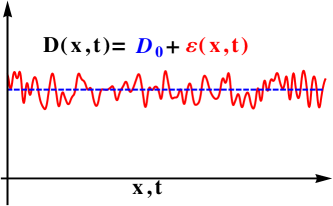
Figure 1: The time and position-dependent diffusion coefficient $D(\textbf{x},t)$ can be decomposed in a constant part $D_{0}$ (blue dashed line) and a fluctuating part $\varepsilon(\textbf{x},t)$ (red continuous line).

Instead of looking for a general solution, we decompose the diffusion coefficient in a constant part $D_{0}$ and a fluctuating part $\varepsilon(\textbf{x},t)$ as shown in Fig. 1, rewriting Eq. 1 as $\partial_{t}I=D_{0}\nabla^{2}I+\nabla\varepsilon(\textbf{x},t)\nabla I$. If both $\varepsilon$ and its gradient are small enough, we can employ a perturbative approach to yield

$$I=g\odot\left[S+\nabla\cdot\varepsilon(\textbf{x},t)\nabla I\right]$$ (2)

where $S(\mathbf{x},t)$ is the source term, $\odot$ represent the convolution product with respect of both the spatial and temporal coordinates defined in $d$ dimensions as

$$f\odot h=\int_{\mathbbm{R}^{d}}d\mathbf{y}\int_{0}^{t}d\tau f\left(\mathbf{x}-\mathbf{y},t-\tau\right)h\left(\mathbf{y},\tau\right),$$

and $g$ is the Green’s function associated to the unperturbed diffusion equation

$$g\left(\mathbf{x},t\right)=\frac{\Theta\left(t\right)}{\sqrt{\left(4\pi D_{0}t\right)^{d}}}e^{-\frac{\mathbf{x}^{2}}{4D_{0}t}},$$

where $\Theta$ is the Heaviside step function. We notice that $g$ is such that $f\odot g=g\odot f$ for every $f$ such that $f\odot g$ exists. For simplicity we will consider only sources terms of the form $S=\delta(\mathbf{x})\delta(t)$. More complicated sources can easily be incorporated, but do not change the general results.

Iterating Eq. 2 we obtain the perturbative series $I=I_{0}+I_{1}+I_{2}+\dots$ where

$$I_{0} =g\odot S=g$$

$$I_{1} =g\odot\left[\nabla\cdot\left(\varepsilon\nabla\left(g\odot S\right)\right)\right]$$

$$=g\odot\left[\nabla\cdot\left(\varepsilon\nabla g\right)\right]$$

$$I_{2} =g\odot\left[\nabla\cdot\left(\varepsilon\nabla\left(g\odot\left(\nabla\cdot\left(\varepsilon\nabla\left(g\odot S\right)\right)\right)\right)\right)\right]$$

$$=g\odot\left[\nabla\cdot\left(\varepsilon\nabla\left(g\odot\left(\nabla\cdot\left(\varepsilon\nabla g\right)\right)\right)\right)\right]$$

$$I_{3} =\dots$$

and we used the fact that $g\odot S=g$.

In order to characterize a possible anomalous scaling of the position variance, we define the $n$th moment along the $x_{i}$ direction of a generic function $f$ as

$$\mu^{(n)}_{x_{i}}\left[f\right]=\int_{-\infty}^{+\infty}\left(x_{i}\right)^{n}f\left(\mathbf{x},t\right)d\mathbf{x}$$

that satisfies these useful properties mellin ; convolutionmoments :

$$\mu^{(n)}_{x_{i}}\left[\partial_{j}f\right]=\left\{\begin{aligned} -&n\mu^{(n-1)}_{x_{j}}\left[f\right]\quad&i=j\\ 0&&i\neq j\end{aligned}\right.$$ (3)

and

$$\mu^{(0)}\left[f\odot g\right] =\mu^{(0)}\left[f\right]\circledast\mu^{(0)}\left[g\right],$$ (4)

$$\mu^{(1)}_{x_{i}}\left[f\odot g\right] =\mu^{(1)}_{x_{i}}\left[f\right]\circledast\mu^{(0)}\left[g\right]+\mu^{(0)}\left[f\right]\circledast\mu^{(1)}_{x_{i}}\left[g\right],$$

$$\mu^{(2)}_{x_{i}}\left[f\odot g\right] =\mu^{(2)}_{x_{i}}\left[f\right]\circledast\mu^{(0)}\left[g\right]+\mu^{(0)}\left[f\right]\circledast\mu^{(2)}_{x_{i}}\left[g\right]+$$

$$+2 \mu^{(1)}_{x_{i}}\left[f\right]\circledast\mu^{(1)}_{x_{i}}\left[g\right]$$

where $\circledast$ represents a convolution product with respect to the sole time variable.

Using these properties we can calculate the zeroth moment for every term in the perturbation:

$$\mu^{(0)}\left[I_{0}\right]=\mu^{(0)}\left[g\right]=1$$

where we used the fact that the Green’s function $g$ is normalized to 1. For the first perturbative order we get

$$\mu^{(0)} \left[I_{1}\right]=\mu^{(0)}\left[g\odot\left(\nabla\cdot\left(\varepsilon\nabla g\right)\right)\right]=\sum_{i=1}^{d}\mu^{(0)}\left[g\odot\partial_{i}\left(\varepsilon\partial_{i}g\right)\right]$$

$$=\sum_{i=1}^{d}\mu^{(0)}\left[\partial_{i}g\odot\left(\varepsilon\partial_{i}g\right)\right]=\sum_{i=1}^{d}\mu^{(0)}\left[\partial_{i}g\right]\circledast\mu^{(0)}\left[\varepsilon\partial_{i}g\right]$$

$$=0$$

where we used the fact that $g$ is an even function and thus $\mu^{(0)}\left[\partial_{i}g\right]=0$. Since the leftmost $g$ and the leftmost $\nabla$ produce a term proportional to $\mu^{(0)}\left[\partial_{i}g\right]$ for every perturbative order, we see that the zeroth moment is non null only for the unperturbed term $I_{0}$. Therefore the perturbative series is correctly normalized at all orders.

Similarly for the first moment we obtain:

$$\mu^{(1)}_{x_{i}}\left[I_{0}\right]=\mu^{(1)}_{x_{i}}[g]=0,$$

$$\mu^{(1)}_{x_{i}}\left[I_{1}\right] =\sum_{j=1}^{d}\mu^{(1)}_{x_{i}}\left[\partial_{j}g\odot\left(\varepsilon\partial_{j}g\right)\right]$$

$$=\sum_{j=1}^{d}\mu^{(1)}_{x_{i}}\left[\partial_{j}g\right]\circledast\mu^{(0)}\left[\varepsilon\partial_{j}g\right].$$

Performing an ensemble average $\left\langle\cdot\right\rangle$ over all possible realization of $\varepsilon$ we obtain

$$\left\langle\mu^{(1)}_{x_{i}}\left[I_{1}\right]\right\rangle=\left\langle\varepsilon\right\rangle\sum_{j=1}^{d}\mu^{(1)}_{x_{i}}\left[\partial_{j}g\right]\circledast\mu^{(0)}\left[\partial_{j}g\right]=0.$$

For the second perturbative term we get:

$$\left\langle\mu^{(1)}_{x_{i}}\left[I_{2}\right]\right\rangle =$$

$$=\left\langle\sum_{j,k=1}^{d}\mu^{(1)}_{x_{i}}\left[\partial_{j}g\odot\left(\varepsilon\left(\partial_{j}\partial_{k}g\odot\left(\varepsilon\partial_{k}g\right)\right)\right)\right]\right\rangle$$

$$=-\left\langle\sum_{i=1}^{d}1\circledast\mu^{(0)}\left[\varepsilon\left(\partial_{i}^{2}g\odot\varepsilon\partial_{i}g\right)\right]\right\rangle$$

$$=-\sum_{i=1}^{d}1\circledast\mu^{(0)}\left[\left(\left\langle\varepsilon\varepsilon\right\rangle\partial_{i}^{2}g\right)\odot\left(\partial_{i}g\right)\right]$$

$$=-\sum_{i=1}^{d}1\circledast\mu^{(0)}\left[\left\langle\varepsilon\varepsilon\right\rangle\partial_{i}^{2}g\right]\circledast\mu^{(0)}\left[\partial_{i}g\right]=0,$$

where we used the fact that, on average, the system is translational invariant in both space and time, and thus $\left\langle\varepsilon(\mathbf{x},t)\varepsilon(\mathbf{x}^{\prime},t^{\prime})\right\rangle=\left\langle\varepsilon\varepsilon\right\rangle\left(|\mathbf{x}-\mathbf{x}^{\prime}|,|t-t^{\prime}|\right)$. We can see that, similarly to what happened for the zeroth moments, the last term in the ensemble averaged first moment can always be written as $\mu^{(0)}\left[\partial_{i}g\right]$. As a consequence, correlations in the disorder at any perturbative order do not change the centre of mass position of $I$.

The calculation of the second moment is more delicate and requires some attention. For the unperturbed term the second moment is trivially

$$\mu^{(2)}_{x_{i}}\left[I_{0}\right]=\mu^{(2)}_{x_{i}}[g]=2D_{0}t.$$

For the first perturbative term we get:

$$\left\langle\mu^{(2)}_{x_{i}}\left[I_{1}\right]\right\rangle =\left\langle\sum_{j=1}^{d}\mu^{(2)}_{x_{i}}\left[\partial_{j}g\odot\left(\varepsilon\partial_{j}g\right)\right]\right\rangle$$

$$=2\left\langle\sum_{j=1}^{d}\mu^{(1)}_{x_{i}}\left[\partial_{j}g\right]\circledast\mu^{(1)}_{x_{i}}\left[\varepsilon\partial_{j}g\right]\right\rangle$$

$$=-2\left(1\circledast\mu^{(1)}_{x_{i}}\left[\left\langle\varepsilon\right\rangle\partial_{i}g\right]\right)$$

$$=-2\left\langle\varepsilon\right\rangle\left(1\circledast\mu^{(1)}_{x_{i}}\left[\partial_{i}g\right]\right)=2\left\langle\varepsilon\right\rangle t.$$

Therefore the average effect of a inhomogeneous and fluctuating diffusion coefficient, up to the first perturbative order, can be captured by using an effective diffusion constant $D_{\text{eff}}=D_{0}+\left\langle\varepsilon\right\rangle$. We can thus safely assume in the following that $\left\langle\varepsilon\right\rangle=0$.

All the averaged moments of the second perturbative order $I_{2}$ depend explicitly on the two-point correlation $\left\langle\varepsilon\varepsilon\right\rangle$, but the second moment is the first one that is not identically zero:

$$\left\langle\mu^{(2)}_{x_{i}}\left[I_{2}\right]\right\rangle =$$ (5)

$$=\left\langle\sum_{j,k=1}^{d}\mu^{(2)}_{x_{i}}\left[\partial_{j}g\odot\left(\varepsilon\left(\partial_{j}\partial_{k}g\odot\varepsilon\left(\partial_{k}g\right)\right)\right)\right]\right\rangle$$

$$=2\left\langle\sum_{j,k=1}^{d}\mu^{(1)}_{x_{i}}\left[\partial_{j}g\right]\circledast\mu^{(1)}_{x_{i}}\left[\varepsilon\left(\partial_{j}\partial_{k}g\odot\varepsilon\partial_{k}g\right)\right]\right\rangle$$

$$=-2\left\langle\sum_{k=1}^{d}1\circledast\mu^{(1)}_{x_{i}}\left[\varepsilon\left(\partial_{i}\partial_{k}g\odot\varepsilon\partial_{k}g\right)\right]\right\rangle$$

$$=-2\sum_{k=1}^{d}1\circledast\mu^{(1)}_{x_{i}}\left[\left(\left\langle\varepsilon\varepsilon\right\rangle\partial_{i}\partial_{k}g\right)\odot\left(\partial_{k}g\right)\right]$$

$$=2\left(1\circledast 1\circledast\mu^{(0)}\left[\left\langle\varepsilon\varepsilon\right\rangle\partial_{i}^{2}g\right]\right)$$

$$=2\int_{0}^{t}\left(t-\tau\right)\left(\int_{\mathbbm{R}^{d}}\left\langle\varepsilon\varepsilon\right\rangle\partial_{i}^{2}g\left(\mathbf{x},\tau\right)\,d\mathbf{x}\right)d\tau$$

where in the last step we used the Cauchy formula for repeated integration.

Eq. 5 shows that the presence of correlations can have an influence on the scaling properties of the second moment. To study the nature and extension of this influence we focus on the 3D case ($d=3$) and assume that the system is not only translational invariant but also isotropic. Eq. 5 can thus be naturally rewritten in spherical coordinates as

$$\mu^{(2)}_{r}\left[\left\langle I_{2}\right\rangle\right]=\frac{8\pi}{3}\int_{0}^{t}\left(t-\tau\right)\left(\int_{0}^{\infty}\left\langle\varepsilon\varepsilon\right\rangle r^{2}\nabla^{2}_{r}g\,dr\right)d\tau,$$ (6)

where $\nabla^{2}_{r}=r^{-2}\partial_{r}r^{2}\partial_{r}$ is the radial part of the Laplacian operator in spherical coordinates.

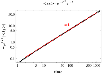
Figure 2: Numerical solution of Eq. 6 for $D_{0}=1$ and $\left\langle\varepsilon\varepsilon\right\rangle=e^{-r^{2}}e^{-t}$ (black dots). Short range (but not vanishing) correlations lead to a contribution to the second moment that scale linearly with time (red dashed line), and thus can be absorbed into an effective diffusion constant.

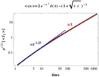
Figure 3: Numerical solution of Eq. 6 for $D_{0}=1$ and $\left\langle\varepsilon\varepsilon\right\rangle=2e^{-r^{2}}\delta(t)-\left(1+\sqrt{rt}\right)^{-1}$ (black dots). The short range term $2e^{-r^{2}}\delta(t)$ give us the correct limit of the correlations when both $r$ and $t$ go to zero, but does not influence $\mu^{(2)}_{x_{i}}\left[\left\langle I_{2}\right\rangle\right]$. The long range anticorrelation term leads to a transient superdiffusive term that scales as $t^{1.25}$ (blue dashed line).

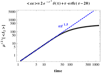
Figure 4: Numerical solution of Eq. 6 for $D_{0}=1$ and $\left\langle\varepsilon\varepsilon\right\rangle=2e^{-r^{2}}\delta(t)+r\operatorname{erfc}(r-20)$ (black dots), where $\operatorname{erfc}$ is the complementary error function that acts as a truncation for the correlations. As in Fig. 3 the short range term is needed to recover the correct limit for $r=t=0$. The rising (but truncated) time-independent correlations leads to a transient superdiffusive term that scales as $t^{1.5}$ (blue dashed line). At long times this contribute saturates to a finite value.

In general we can write the 2-point correlation as $\left\langle\varepsilon\varepsilon\right\rangle=\left\langle\varepsilon^{2}\right\rangle h\left(r,\tau\right)$ where $\left\langle\varepsilon^{2}\right\rangle$ represents the variance of the diffusion coefficient’s fluctuations (that we will set to 1 unless explicitly stated), and $h\left(r,\tau\right)$ is a distribution that describe the shape of the correlations. In order to be physical we require $h$ to go to zero when either $r$ or $\tau$ go to infinity, and to go to 1 (or to a Dirac delta) when both $r$ and $\tau$ go to zero. If the time fluctuations of $\varepsilon$ are well represented by white noise, then $\left\langle\varepsilon\varepsilon\right\rangle\propto\delta(\tau)$. Since $\lim_{t\rightarrow 0}\nabla^{2}g=0$ there will be no contribution to the second moment. More complicated functional forms for the two-point correlations require a numerical integration of Eq. 6.

The effect of a given form for the correlations can be categorized in a limited numbers of cases.

1. It can produce a null contribution.

2. It can produce a contribution that scale linearly with time (either positive or negative). In this case the effect can be absorbed in the effective diffusion constant $D_{\text{eff}}$.

3. It can produce a contribution that grows slower than linearly. In this case the contribution from the unperturbed term is always bigger than the one due to the correlations, and thus it is negligible.

4. It can produce a contribution that grows faster than linearly. In this case the overall transport is effectively superdiffusive.

Not surprisingly we find that short range correlations always yield one of the first 3 cases. A typical example is shown in Fig. 2.

For long range correlations of the form $\left\langle\varepsilon\varepsilon\right\rangle\propto r^{a}t^{b}$, Eq. 6 can be integrated to give $\mu^{(2)}_{x_{i}}\left[\left\langle I_{2}\right\rangle\right]\propto t^{1+b+a/2}$. If at least one of $a$ or $b$ is positive then the transport can be superdiffusive. It is interesting to notice that if we allow $\left\langle\varepsilon^{2}\right\rangle$ to grow polynomially with time, the position variance can grow as fast as we want, even faster than the ballistic $t^{2}$ case. Of course increasing the fluctuations requires a steady influx of energy into the system and therefore an accelerated transport regime is not an impossibility. Furthermore, sooner or later the growing fluctuations will violate the assumptions behind our perturbative approach and thus this result can not be extrapolated to the large time limit. Since $\left\langle\varepsilon\varepsilon\right\rangle$ can not grow indefinitively, neither $a$ or $b$ can be positive at large time or large distances. This results in a diffusive transport in the long time limit. This does not mean that there can not be a transient superdiffusive regime similar to the one encountered in truncated Lévy walks mantegna . Fig 3 shows the transient superdiffusive transport where the second moment grows as $t^{1.25}$ due to a (anti)correlation that decays asymptotically as $(\sqrt{rt})^{-1}$. Finally, while it is true that the correlation function can not grow indefinitely, if we truncate it after a certain distance/time we obtain again a transient superdiffusive transport, as shown in Fig. 4.

In conclusion we showed that correlations in the diffusion coefficient fluctuations can lead to a transient superdiffusive behavior, and found an explicit formula to link the two-point correlation $\left\langle\varepsilon\varepsilon\right\rangle$ with the time scaling of the position variance. The higher order perturbation terms depend on the three-point correlation $\left\langle\varepsilon\varepsilon\varepsilon\right\rangle$, four-point correlation $\left\langle\varepsilon\varepsilon\varepsilon\varepsilon\right\rangle$ and so on, that can also lead to deviations from a standard diffusive transport.

References

(1)
J. Fourier, Théorie analytique de la chaleur (Firmin Didot Père et
Fils, Paris, 1822).
(2)
H.A. Kramers, Physica 7, 284 (1940).
(3)
P. Sheng, Introduction to Wave Scattering, Localization and Mesoscopic
Phenomena (Springer, 2010).
(4)
F. Martelli, S. Del Bianco, A, Ismaelli, G. Zaccanti, Light Propagation
Through Biological Tissue and Other Diffusive Media (SPIE Press, 2009).
(5)
E. Akkermans and G. Montambaux, Mesoscopic Physics of Electrons and
Photons (Cambridge University Press, 2007).
(6)
L. J.-B. A. Bachelier, Ann. Sci. Ec. Norm. Sup. 3 21 (1900).
(7)
F. Black and M. Scholes, J. Polit. Econ. 81, 637 (1973).
(8)
B. V. Gnedenko and A. N. Kolmogorov, Limit Distributions for Sums of
Independent Random Variables (Addison-Wesley, 1954).
(9)
K. Pearson and J. W. Strutt, Nature 72, 294; 318; 342 (1905).
(10)
A. Einstein, Investigations on the Theory of the Brownian Movement
edited by R. Furth (Dover Publications, New York, 1998).
(11)
R. Klages, G. Radons, and I. M. Sokolov, Anomalous Transport
(Wiley-VCH, 2008); R. Metzler, and J. Klafter, Phys. Rep. 339, 1
(2000).
(12)
R. Metzler and J. Klafter, J. Phys. A: Math. Gen. 37, R161 (2004).
(13)
T. H. Solomon, E. R. Weeks, and H. L. Swinney, Phys. Rev. Lett. 71,
3975 (1993).
(14)
A. Corral, Phys. Rev. Lett. 97, 178501 (2006).
(15)
P. Barthelemy, J. Bertolotti, and D. S. Wiersma, Nature 453, 495
(2008).
(16)
N. Mercadier, W. Guerin, M. Chevrollier, and R. Kaiser, Nature Phys. 5,
602 (2009).
(17)
R. Metzler and J. Klafter, Phys. Rep. 339, 1 (2000).
(18)
A. Fick, Ann. der. Physik 94, 59 (1855).
(19)
R. I. Hickson, S. I. Barry, G. N. Mercer, Int. J. Heat Mass Tran. 52,
5776 (2009).
(20)
A. D. Poularikas, Handbook of Formulas and Tables for Signal
Processing (Springer, 1999).
(21)
C. A. Laury-Micoulaut, Astron. Astrophys. 51 343 (1976).
(22)
R. N. Mantegna and H. E. Stanley, Phys. Rev. Lett. 73, 2946 (1994).