Locality of the Aharonov-Bohm-Casher effect

Abstract

We address the question of the locality versus nonlocality in the Aharonov-Bohm and the Aharonov-Casher effects. For this purpose, we investigate all possible configurations of ideal shielding of the overlap between the electromagnetic fields generated by a charge and by a magnetic flux, and analyze their consequences on the Aharonov-Bohm-Casher interference. In a classical treatment of shielding, the Aharonov-Bohm-Casher effect vanishes regardless of the geometry of shielding, when the local overlap of electromagnetic fields is completely eliminated. On the other hand, the result depends on the configuration of shielding if the charge quantization in the superconducting shield is taken into account. It is shown that our results are fully understood in terms of the fluctuating local-field interaction. Our analysis strongly supports the alternative view on the Aharonov-Bohm-Casher interference that the effects originate from the local action of electromagnetic fields.

I introduction

It is a widely accepted view that the Aharonov-Bohm (AB) effect Aharonov and Bohm (1959), which describes the quantum interference of a charged particle moving in a region free of electromagnetic fields, is a pure topological phenomenon that cannot be understood from the local action of fields. In contrast to this common viewpoint, we have recently shown that a fully local description of the force-free AB effect is possible based on the Lorentz-invariant interactions of electromagnetic fields Kang (2013). Naturally, this resolves a long-standing puzzle on why the old local-interaction-based theories Liebowitz (1965); Boyer (1973); Spavieri and Cavalleri (1992) have failed to provide a consistent description of the force-free AB effect: The relativity principle was not properly taken into account in the previous field-interaction-based theories, and neglecting the Lorentz invariance gives rise to erroneous classical forces. An immediate and important corollary of the local-interaction-based framework is that the AB effect vanishes if all local overlap of electromagnetic fields is shielded. The purpose of this paper is to provide an extensive investigation on the effect of shielding and its consequences on the AB effect and the Aharonov-Casher(AC) effect Aharonov and Casher (1984) - a dual phenomenon to the AB effect.

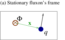
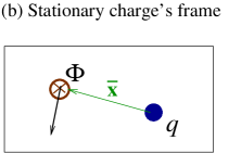
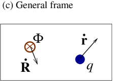
Figure 1: A charge $q$ and a fluxon $\Phi$ moving in two spatial dimension in (a) the stationary fluxon’s frame, (b) the stationary charge’s frame, and (c) a general frame, respectively.

The main question raised concerning the standard nonlocal viewpoint can be clearly stated as follows, which was already noticed in Ref. Reznik and Aharonov, 1989. Let us consider a charge ($q$) and a fluxon ($\Phi$) in 2+1 dimension (Fig. 1). The principle of relativity demands that the physical law governing the system be independent of the reference frame. The AB effect is described in the frame of the stationary fluxon, $O_{\Phi}$ (Fig.1(a)). The AB phase shift is induced by the charge encircling the fluxon. The standard viewpoint on this phenomenon is that it is purely topological and originates from the nonlocal interaction of the charge and the fluxon, described by the “nonlocal” Lagrangian

$$L_{i}^{nl}=\frac{q}{c}\dot{\mathbf{x}}\cdot\mathbf{A}(\mathbf{x}),$$ (1)

where $\mathbf{x}$ and $\mathbf{A}(\mathbf{x})$ are the position of the charge relative to the fluxon and the vector potential generated by the fluxon, respectively. The “nonlocality” here implies that the charge and the magnetic field do not experience a direct local interaction. In this framework, the AB effect is purely topological in that it requires that the charge be confined in a multiply connected region and in that there is no realistic way to relate a phase shift to any particular position in the charge’s path.

On the other hand, in the stationary charge’s reference frame, $O_{q}$ (Fig.1(b)), the moving fluxon acquires a phase shift via the local interaction Lagrangian

$$L_{i}^{l}=\frac{\dot{\bar{\mathbf{x}}}}{4\pi c}\cdot(\Phi\hat{z})\times\mathbf{E}(\bar{\mathbf{x}}),$$ (2)

where $\hat{z}$ is the unit vector perpendicular to the plane, and $\bar{\mathbf{x}}=-\mathbf{x}$ is the position of the fluxon relative to the charge. $\mathbf{E}(\bar{\mathbf{x}})$ is the electric field generated by the charge at the location of the fluxon. The phase shift that appears in this reference frame is known as the AC effect Aharonov and Casher (1984). It can be understood in terms of the local-interaction-induced accumulation of the phase shift, although it is rarely noticed. The locality of the AC effect was also demonstrated in Ref. Peshkin and Lipkin, 1995.

In two spatial dimension, however, the AB and the AC effects are actually the same phenomena - only their reference frames are different. The duality of the two phenomena is demonstrated by the equality of the phase accumulated by one loop rotation derived in each frame:

$$\varphi=\frac{q}{\hbar c}\oint\mathbf{A}(\mathbf{x})\cdot d\mathbf{x}=\frac{\Phi}{4\pi\hbar c}\oint\hat{z}\times\mathbf{E}(\bar{\mathbf{x}})\cdot d\bar{\mathbf{x}}=\frac{q\Phi}{\hbar c}\,.$$ (3)

In spite of this equality, the result would be interpreted differently for the two observers in the frames $O_{\Phi}$ and $O_{q}$, respectively. Intriguingly, third observer ($O^{\prime}$), who finds that both particles are moving (Fig. 1(c)), would be frustrated with the two contradictory interpretations. This observer cannot even decide with which Lagrangian, Eq.(1) or Eq.(2), to start. As noticed in Ref. Reznik and Aharonov (1989), there would be two possible resolutions to this inconsistency: Either (i) the AC effect should be interpreted as a nonlocal and purely topological effect or (ii) the AB effect is a result of local interaction. The common attitude to this problem is to ignore the paradox, or, to regard possibility (i) as the solution, which has also been argued in Ref. Reznik and Aharonov, 1989 for a particular arrangement of the AC setup.

In this paper, in contrast to the common notion, we show that resolution (ii) is possible and that it provides a more universal framework independent of the reference frame. Introducing various types of shielding the overlap of electromagnetic fields, we show that the AB effect vanishes if the local interaction of the fields is completely eliminated. Our results strongly support the validity of the alternative local-interaction-based theory of the Aharonov-Bohm-Casher (ABC) effect.

The paper is organized as follows. First, the field-interaction-based Lagrangian and Hamiltonian are introduced for a charge and a fluxon in two dimension (Section II). In Section III, a classical treatment of ideal shielding is briefly discussed, and it is shown that the ABC interference disappears if the local overlap of the fields produced by the two particles vanishes. Then, we provide an extensive quantum mechanical treatment in the presence of superconducting barriers placed in between the charge and the fluxon (Section IV). The result depends on the specific configuration of the system, whereas we find that the ABC effect is determined by the fluctuating local field interaction in general. The implications of the results in Sections III and IV are summarized and discussed in Section V. Our conclusion is given in Section VI.

II Field-interaction Lagrangian for a charge and a fluxon

The simplest case that can be conceived for describing the ABC effect is a two-particle system of a charge $q$ and a fluxon $\Phi$ at locations of $\mathbf{r}$ and $\mathbf{R}$, respectively. Our starting point is to introduce the universal Lorentz-covariant field interaction Lagrangian for describing the interaction between the two particles Kang (2013). An obvious merit of this approach is that we do not have to worry about choosing which of the two pictures, nonlocal (Eq. (1)) or local (Eq. (2)), as our starting point. In the limit of $\dot{r},\dot{R}\ll c$, the Lagrangian of the system is given by Kang (2013)

$$L=\frac{1}{2}m\dot{\mathbf{r}}\cdot\dot{\mathbf{r}}+\frac{1}{2}M\dot{\mathbf{R}}\cdot\dot{\mathbf{R}}+L_{\rm int},$$ (4a)

where $$m M L_{\rm int}$$() is the mass of the charge(fluxon). The interaction between the two particles, , is derived from the Lorentz-covariant field interactions Kang (2013) as

$$L_{\rm int}=\frac{1}{4\pi}\int\left(\mathbf{B}_{q}\cdot\mathbf{B}_{\Phi}-\mathbf{E}_{q}\cdot\mathbf{E}_{\Phi}\right)\,d\tau\,,$$ (4b)

where $$\mathbf{B}_{q} \mathbf{E}_{q} \mathbf{B}_{\Phi} \mathbf{E}_{\Phi}$$() and () are the magnetic(electric) fields produced by the charge and by the fluxon, respectively. Note that this Lagrangian is uniquely constructed from the obvious first principles of (i) relativity, (ii) linearity in the field strengths, and (iii) correspondence with the known result in the limit of stationary charge Kang (2013). One can rewrite Eq. (4b) in the simpler form

$$L_{\rm int}=(\dot{\mathbf{r}}-\dot{\mathbf{R}})\cdot\mathbf{\Pi}\,,$$ (4c)

with the field momentum $$\mathbf{\Pi}$$ produced by the overlap of charge’s electric field and the fluxon’s magnetic field:

$$\mathbf{\Pi}=\frac{1}{4\pi c}\int\mathbf{E}_{q}\times\mathbf{B}_{\Phi}d\tau\,.$$ (4d)

Note that Eq. (4c) is equivalent to the interaction Lagrangian

$$L_{\rm int}=\frac{q}{c}(\dot{\mathbf{r}}-\dot{\mathbf{R}})\cdot\mathbf{A}\,,$$ (4e)

based on the vector potential $$\mathbf{A}$$, except that in the former case (Eq. (4c)), the Lagrangian is given only by the gauge-independent physical quantities.

This Lagrangian (Eq. 4) can also be transformed to the Hamiltonian

$$H=\frac{1}{2m}\left(\mathbf{p}-\mathbf{\Pi}\right)^{2}+\frac{1}{2M}\left(\mathbf{P}+\mathbf{\Pi}\right)^{2}\,,$$ (5)

where $\mathbf{p}$ and $\mathbf{P}$ are the canonical momenta of the charge and the fluxon, respectively. A noticeable point about these canonical momenta is that they are physical quantities given by

$$\mathbf{p}=m\dot{\mathbf{r}}+\mathbf{\Pi},\;\;\;\mathbf{P}=M\dot{\mathbf{R}}-\mathbf{\Pi},$$ (6)

contrary to their gauge dependence in the standard potential-based model. The canonical momentum of charge, $\mathbf{p}$, is the sum of the mechanical ($m\dot{\mathbf{r}}$) and the field ($\mathbf{\Pi}$) momenta. The canonical momentum of the fluxon, $\mathbf{P}$, can be interpreted as the sum of the translational ($M\dot{\mathbf{R}}$) and the hidden relativistic Aharonov et al. (1988) mechanical momenta. In both cases, the canonical momenta are the net momenta carried by each particle.

It has previously been shown Kang (2013) that this local-interaction-based Lagrangian (Hamiltonian) of Eq. (4) (Eq. (5)) reproduces the main features of the ABC effect; (i) the absence of the classical mechanical force and (ii) the appearance of the topological phase $\varphi$ (formed by the local accumulation of the field momentum in our framework),

$$\varphi=\frac{1}{\hbar}\oint\mathbf{\Pi}\cdot d\mathbf{r}=q\Phi/\hbar c\,.$$ (7)

III Classical treatment of shielding

To answer the question of locality versus nonlocality of the ABC effect, it is essential to investigate the case where local overlap of the electromagnetic fields is eliminated. For this purpose, we consider three possible configurations of shielding (Fig. 2). In all cases, an ideal Faraday cage is placed between the charge and the fluxon. We adopt the local-interaction-based Lagrangian and Hamiltonian of Eqs. (4) and (5) for this analysis, but it should be noted that the standard potential-based description leads to the same result. Note that the shielding configuration realized in the experiment of Ref. Tonomura et al., 1986 cannot be applied to our analysis here because of the nonadiabatic nature of the field generated by the incident electrons with high kinetic energy Kang (2013). (This point will be discussed in Section V.)

Let us first analyze the induced ABC phase in the presence of an ideal classical conductor placed between the two particles. Quantum treatments for superconducting shields will be provided in the next section. In any configuration of the two particles and a conducting shield (Fig. 2), the interactions are governed by the overlaps among the electromagnetic fields produced by the charge, the fluxon, and the conducting shield. The only constraint imposed here is that the induced charge density in the conducting shield generates an electric field ($\mathbf{E}_{s}$) that compensates for the field of the charge flo . Then, we find the net interaction Lagrangian as

$$L_{\rm int}=\frac{1}{4\pi}\int\left[(\mathbf{B}_{q}+\mathbf{B}_{s})\cdot\mathbf{B}_{\Phi}-(\mathbf{E}_{q}+\mathbf{E}_{s})\cdot\mathbf{E}_{\Phi}\right]\,d\tau+L_{qs}\,,$$ (8)

where $\mathbf{B}_{s}$($\mathbf{E}_{s}$) is the magnetic(electric) field generated by the induced charge in the superconductor. $L_{qs}$, which represents the interaction between the charge $q$ and the conducting shield, is irrelevant to the ABC effect. For an ideal classical conductor, the electric and magnetic fields generated by charge $q$ are exactly canceled by the induced charges in the conducting shield, that is, $\mathbf{E}_{q}+\mathbf{E}_{s}=0$ and $\mathbf{B}_{q}+\mathbf{B}_{s}=0$, at the location of the fluxon. Therefore, the interaction Lagrangian of Eq. (8) is independent of the localized magnetic flux, and accordingly the ABC effect vanishes. Note that this conclusion is valid also in the potential-based treatment Kang (2013), which has been widely overlooked.

IV Quantum treatment of shielding

In the previous section, we have shown that the ABC phase shift vanishes in the classical treatment of ideal shielding, independent of the geometry considered in Fig. 2. Whereas this already demonstrates the locality of the ABC effect, it is important to test the validity of the locality with a quantum mechanical treatment of the conducting shield. In the following, we show that the effect of shielding depends on the geometry of the system, when we take into account the quantization of charges in the superconductor. For a quantum treatment, we consider an ideal superconductor placed in between the charge and the fluxon. Ideal shielding in the quantum treatment implies that the quantum mechanical average values of the net electric and magnetic fields, generated by charge $q$ and the induced charges in the superconductor, vanish at the location of the fluxon.

IV.1 Configuration I: Fluxon confined in a superconductor

In Configuration I (Fig. 2(a)), the fluxon is confined inside the superconducting Faraday cage, and the charge is moving in the region outside the superconductor. Here we use the potential-based theory for convenience, but as we have already pointed out in the previous section, the same conclusion is drawn from the field-interaction-based framework. The Lagrangian of the system is given by

$$L=\frac{m}{2}\dot{\mathbf{r}}\cdot\dot{\mathbf{r}}+L_{\rm sc}+L_{\rm int}\,,$$ (9a)

where $$L_{\rm sc}$$ describes the superconductor, and the interaction term

$$L_{\rm int}=\frac{q}{c}\dot{\mathbf{r}}\cdot\mathbf{A}+\frac{1}{c}\int\delta n(\phi)\,\mathbf{v}_{c}\cdot\mathbf{A}\,d\mathbf{r}^{\prime},$$ (9b)

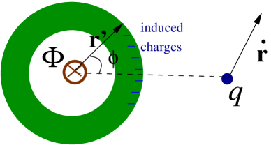
Figure 3: The structure of the shielding in Configuration I of Fig. 2(a).

is composed of two parts: The first term is the main interaction between the charge $q$ and the fluxon; the second term represents the interaction between the superconductor and the fluxon. The moving charge $q$ induces a variation of the surface charge density, $\delta n(\phi)$, on the outer surface of the superconductor moving with velocity $\mathbf{v}_{c}$. $\delta n(\phi)$ depends on the azimuthal angle $\phi$ of the position vector $\mathbf{r}^{\prime}$ on the surface (see Fig. 3). The interaction between charge $q$ and the superconductor, which is irrelevant to the ABC phase shift, is neglected here.

The transition amplitude of the moving charge $q$ from a point $(\mathbf{r}_{i},t_{i})$ to another $(\mathbf{r}_{f},t_{f})$ in spacetime is given by

$$u_{i\rightarrow f} = \langle\mathbf{r}_{f}|\otimes\langle\eta_{f}|e^{-iH(t_{f}-t_{i})/\hbar}|\mathbf{r}_{i}\rangle\otimes|\eta_{i}\rangle$$

$$= \lim_{M\rightarrow\infty}\langle\mathbf{r}_{f}|\otimes\langle\eta_{f}|\left(e^{-iH\epsilon/\hbar}\right)^{M}|\mathbf{r}_{i}\rangle\otimes|\eta_{i}\rangle,$$

where $|\eta_{i}\rangle$ ($|\eta_{f}\rangle$) denotes the initial (final) state of the superconducting shield, and $\epsilon\equiv(t_{f}-t_{i})/M$. The state of the superconducting shield can be written as

$$|\eta\rangle=\sum_{m}b_{m}|\psi_{m}\rangle\,,$$ (11)

where $|\psi_{m}\rangle$ stands for a substate with $m$ excess Cooper pairs on the outer surface of the superconductor. The state $|\psi_{m}\rangle$ satisfies

$$\int d\mathbf{r}^{\prime}\langle\psi_{m}|n(\phi)|\psi_{m}\rangle=2em,$$ (12)

that is, the induced charge is quantized in units of 2e.

The transition amplitude of Eq. (IV.1) should be evaluated by taking into account all possible trajectories of the charge $q$ and the superconductor. In our case, we are interested only in the paths in which, inside the cage, the electric and the magnetic fields generated by the charge $q$ are perfectly shielded by the induced charges in the superconductor. The question here is whether this condition is fulfilled in the presence of quantization of the induced charges (by $2em$). One can find that this is indeed the case, and the electric and the magnetic fields inside the cage vanish for any number $m$ of excess Cooper pairs, if and only if

$$\langle\psi_{m}|n(\phi)|\psi_{m}\rangle=n_{0}^{m}+\delta n(\phi),$$ (13a)

where $$n_{0}^{m}=(2em+q)/2\pi R R$$ ( being the outer radius of the superconductor) is a constant, and the inhomogeneous part,

$$\delta n(\phi)=-\frac{q}{2\pi R}\left(\frac{r^{2}-R^{2}}{r^{2}+R^{2}-2rR\cos{\phi}}\right)$$ (13b)

provides perfect shielding of the fields. The transition amplitude of Eq. (IV.1), with the above condition (Eq. (13b)) for the superconducting barrier, can be rewritten in the form

$$u_{i\rightarrow f}=\int_{\mathbf{r}_{i}}^{\mathbf{r}_{f}}{\cal D}[\mathbf{r}(t)]\exp{\left\{\frac{i}{\hbar}\int L(\mathbf{r},\dot{\mathbf{r}},t)\right\}}\,,$$ (14)

where the Lagrangian is given by Eq. (9b). For this path integration, we are summing all contributions satisfying the condition of Eq. (13b). In this case, one can find that the first and the second terms of Eq. (9b) are given by $q\Phi\dot{\phi}/(2\pi c)$ and $-q\Phi\dot{\phi}/(2\pi c)$, respectively, which cancel each other. Therefore, $L_{\rm int}=0$, and the fluxon does not contribute to the phase factor of $u_{i\rightarrow f}$. The ABC effect vanishes completely in this configuration.

IV.2 Configuration II: Charge confined in a superconducting cage

Now we turn our attention to Configuration II (Fig. 2(b)), where the charge is confined inside the cage and the fluxon is located outside. We consider only a grounded superconductor flo where the field produced by the charge cannot penetrate outside the shield. As we will show in the following, quantum fluctuation of charge is essential in this configuration (and also in Configuration III).

For convenience, we adopt the stationary charge’s frame ($O_{q}$). The transition amplitude of a moving fluxon is given in the same way as in Eq. (IV.1),

$$u_{i\rightarrow f}=\lim_{M\rightarrow\infty}\langle\mathbf{R}_{f}|\otimes\langle\eta_{f}|\left(e^{-iH\epsilon/\hbar}\right)^{M}|\mathbf{R}_{i}\rangle\otimes|\eta_{i}\rangle,$$ (15)

where the Hamiltonian is given by

$$H=\frac{1}{2M}(\mathbf{P}+\mathbf{\Pi})^{2}+H_{0}\,.$$ (16)

Here $H_{0}$ denotes the contribution from the superconducting condensate and the interaction between charge $q$ and the superconductor. $H_{0}$ does not contribute to the ABC phase and so is ignored here. The field momentum $\mathbf{\Pi}$ is produced by the overlap of the net electric field of the charges and the magnetic field of the fluxon ($\mathbf{B}_{\Phi}$) as

$$\mathbf{\Pi}=\frac{1}{4\pi c}\int(\mathbf{E}_{q}+\mathbf{E}_{s})\times\mathbf{B}_{\Phi}d\tau\,,$$ (17)

where $\mathbf{E}_{q}$ and $\mathbf{E}_{s}$ denote the electric fields generated by charge $q$ and by the superconductor, respectively. The expectation value of $\mathbf{E}_{s}$ depends on the state of the superconducting shield, $|\eta\rangle$, given as a coherent superposition of the number eigenstates $|\psi_{m}\rangle$ as in Eq. (11), where $m$ denotes the excess number of induced Cooper pairs on the surface of the superconductor. Ideal shielding of the fields in quantum treatment is imposed by the condition

$$\langle\eta|\mathbf{E}_{q}+\mathbf{E}_{s}|\eta\rangle=0\,.$$ (18)

An intriguing point here is that, although the expectation value of the field vanishes for the ideal superconductor, this perfect shielding cannot be achieved for any particular substate with definite number $m$, $|\psi_{m}\rangle$, unless $q$ is an integer multiple of $2e$. That is, $\langle\psi_{m}|\mathbf{E}_{q}+\mathbf{E}_{s}|\psi_{m}\rangle\neq 0$, in general. This is the major difference from Configuration I where the field interaction vanishes for any number $m$ of excess Cooper pairs. Therefore, in contrast to Configuration I, the charge-fluxon interaction is not completely suppressed, and the transition amplitude is reduced to

$$u_{i\rightarrow f}=\sum_{ml}b_{m}b_{l}^{*}u_{lm}(f;i)\,,$$ (19a)

where

$$u_{lm}(f;i) = \langle\mathbf{R}_{f}|\otimes\langle\psi_{l}|e^{-\frac{i}{\hbar}H(t_{f}-t_{i})}|\mathbf{R}_{i}\rangle\otimes|\psi_{m}\rangle$$ (19b)

$$= \int_{\mathbf{R}_{i}}^{\mathbf{R}_{f}}{\cal D}[\mathbf{R}(t)]e^{\frac{i}{\hbar}\int L_{lm}(\mathbf{R},\dot{\mathbf{R}})dt}\,.$$

$$L_{lm}$$, the element of the moving fluxon’s Lagrangian, is found to be

$$L_{lm}(\mathbf{R},\dot{\mathbf{R}})=\left(\frac{M}{2}\dot{R}^{2}-\dot{\mathbf{R}}\cdot\mathbf{\Pi}_{m}\right)\delta_{lm}\,,$$ (19c)

where $$\mathbf{\Pi}_{m}=\langle\psi_{m}|\mathbf{\Pi}|\psi_{m}\rangle |\psi_{m}\rangle$$ is the field momentum for the particular state . For a fluxon with a negligible size, we find

$$\mathbf{\Pi}_{m}=-\frac{q+2em}{2\pi cR}\Phi\hat{\phi},$$ (19d)

and the phase factor acquired for one-loop rotation induced by the interaction term is

$$u_{1}=\sum_{m}|b_{m}|^{2}e^{i\varphi_{m}},$$ (20a)

where the phase shift $$\varphi_{m} |\psi_{m}\rangle$$ for a particular substate is induced by the local field interaction as

$$\varphi_{m}=-\frac{1}{\hbar}\oint\mathbf{\Pi}_{m}\cdot d\mathbf{R}=\frac{(q+2em)\Phi}{\hbar c}\,.$$ (20b)

Unlike Configuration I, the ABC effect is not completely shielded but modified by the superconductor. The change of the phase factor is manifested by the fluctuating local field interaction represented by the term $$-\dot{\mathbf{R}}\cdot\mathbf{\Pi}_{m} u_{1} \{|b_{m}|\}$$ in Eq. (19c). The phase factor in Eq. (20a) depends on the coefficients , with a constraint imposed by the condition of complete shielding (Eq. (18)),

$$\sum_{m}m|b_{m}|^{2}=-q/2e\,.$$ (20c)

IV.3 Configuration III: Both particles confined in a superconductor

A particularly interesting limit in the result of the previous section is found when $\Phi$ is quantized in units of superconducting flux quantum, $\Phi=(hc/2e)\times\rm{integer}$. In fact, this quantization is achieved for Configuration III. In this case, the phase factor of Eq. (20a) is reduced to

$$u_{1}=e^{iq\Phi/\hbar c}.$$ (21)

That is, the ABC effect is unaffected by the presence of the superconducting shield, in spite of complete shielding of the (expectation value of) the electromagnetic fields. This case was analyzed in Ref. Reznik and Aharonov, 1989. Based on this result, the authors in Ref. Reznik and Aharonov, 1989 argued that the AC effect also represents a nonlocal interaction, although it appears as a local interaction of Eq. (2), and concluded that the nonlocal picture should be applied in both the AB and the AC effects. It is clear from our study that this is an incomplete argument. Configuration III is only a special case of shielding the local field interactions, and one cannot draw a general conclusion that the ABC effect is understood only in terms of the nonlocal picture. Our analysis of the three possible different configurations shows that the effect of shielding is not very universal but depends on the type of shielding, and that the result is determined by the fluctuating local field interactions.

V Discussion

The results of our analysis on shielding the local interaction of fields are summarized as follows. First, there is a qualitative difference between classical and quantum treatments. In the classical approach to shielding, the local field interactions are completely suppressed as far as the shielding of the field is ideal, and this eliminates the ABC effect. In the quantum treatment of shielding where the charge quantization is taken into account in the superconducting shield, two different types appear depending on the geometry of shielding. The shielding of the electromagnetic field eliminates the ABC effect in Configuration I (Fig. 2(a)), whereas the shielding does not completely suppress the effect in Configurations II and III (Figs. 2(b) and (c)). The main difference between these two classes is the role of the fluctuating local field interactions. In Configurations II and III, although the expectation value of the field generated by charge $q$ is compensated for by that of the induced charge in the superconductor, the field interactions are not completely suppressed. The ABC effect is modified (in Configuration II) or even unaffected (in Configuration III) in spite of an ideal shielding of the charge’s field in the position of the fluxon. We can conclude that this is due to the fluctuating local field interactions, and that it demonstrates the locality of the electromagnetic interaction in Aharonov-Bohm-Casher interferometry.

Experimentally, no experiments so far have been performed under the condition of perfect shielding of the field interactions. The most ideal one was the experiment performed by Tonomura et al. Tonomura et al. (1986), where the magnetic flux is shielded by a superconductor from the moving electron’s path. Their setup is basically equivalent to Configuration I where the flux is confined in a superconducting shield. Contrary to the analysis for Configuration I, a clear AB phase shift was observed despite the presence of the superconducting shield. In this experiment, however, incident electrons with a speed of about $2.4\times 10^{8}\rm{m/s}$ were used. In fact, no superconducting material can shield the magnetic field produced by such fast electrons Kang (2013), and the ideal shielding analysis in Section IV-A cannot be applied to the experiment in Ref. Tonomura et al., 1986. In other words, the shielding in the experiment of Ref. Tonomura et al., 1986 was only one-sided where the incident electron is moving in a field-free region, whereas shielding of both sides is necessary to eliminate the Aharonov-Bohm effect. The experimental result of Ref. Tonomura et al., 1986 can be fully understood in the framework of the local field interaction between the localized flux and the magnetic field produced by an incident electron.

VI Conclusion

A local-interaction-based theory of the ABC effect has recently been formulated Kang (2013); this theory is consistent with all the results predicted in the standard potential-based framework. To verify the local nature of the ABC effect, we have investigated the interaction of a charge and a fluxon when an ideal conducting barrier is placed between the two objects. In the classical treatment of shielding, the ABC effect vanishes in the absence of the overlap of electromagnetic fields for any geometry of the system. In quantum treatments of superconducting barriers, however, the result depends on the geometry of the system. The superconducting shield suppresses the ABC interference completely in Configuration I (Fig. 2(a)). In contrast, the ABC phase factor is modified in Configuration II, or even unaffected in Configuration III. We have shown that the effect of shielding is determined by the fluctuating local interaction of the electromagnetic fields. Our study shows that the framework of local field interaction is fully adequate for a universal description of the ABC effect.

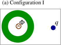
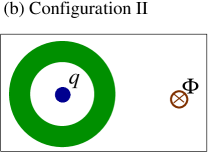
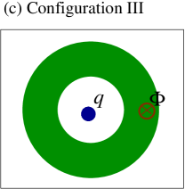
Figure 2: Three possible configurations of shielding the overlap of the electromagnetic fields produced by charge $q$ and fluxon $\Phi$. Green regions represent the superconducting barriers.

References

- Aharonov and Bohm (1959) Y. Aharonov and D. Bohm, Phys. Rev. 115, 485 (1959).
- Kang (2013) K. Kang, (2013), arXiv:1308.2093 [quant-ph] .
- Liebowitz (1965) B. Liebowitz, Il Nuovo Cimento Series 10 38, 932 (1965).
- Boyer (1973) T. H. Boyer, Phys. Rev. D 8, 1679 (1973).
- Spavieri and Cavalleri (1992) G. Spavieri and G. Cavalleri, Europhys. Lett. 18, 301 (1992).
- Aharonov and Casher (1984) Y. Aharonov and A. Casher, Phys. Rev. Lett. 53, 319 (1984).
- Reznik and Aharonov (1989) B. Reznik and Y. Aharonov, Phys. Rev. D 40, 4178 (1989).
- Peshkin and Lipkin (1995) M. Peshkin and H. J. Lipkin, Phys. Rev. Lett. 74, 2847 (1995).
- Aharonov et al. (1988) Y. Aharonov, P. Pearle, and L. Vaidman, Phys. Rev. A 37, 4052 (1988).
- Tonomura et al. (1986) A. Tonomura, N. Osakabe, T. Matsuda, T. Kawasaki, J. Endo, S. Yano, and H. Yamada, Phys. Rev. Lett. 56, 792 (1986).
- (11) An exceptional case is Configuration II with a floating superconductor. In this case, the electric field of the charge is not compensated by the superconductor and extends to the location of the fluxon. Therefore, this is irrelevant to our analysis, and we consider only a grounded superconductor that perfectly shields the fields.