Abstract

Voigt wave propagation was investigated in a homogenized composite material (HCM) arising from a porous electro–optic host material infiltrated by a fluid of refractive index $n_{a}$. The constitutive parameters of the HCM were estimated using the extended Bruggeman homogenization formalism. Numerical studies revealed that the directions which support Voigt wave propagation in the HCM could be substantially controlled by means of an applied dc electric field. Furthermore, the extent to which this control could be achieved was found to be sensitive to the porosity of the host material, the shapes, sizes and orientations of the pores, as well as the refractive index $n_{a}$. These findings may be particularly significant for potential technological applications of Voigt waves, such as in optical sensing.

Keywords: Voigt waves, electro–optic materials, Bruggeman homogenization formalism, Pockels effect

1 Introduction

The setting for this numerical study is electromagnetic plane–wave propagation in anisotropic dielectric materials. Usually in such materials two plane waves with different phase speeds and orthogonal polarizations propagate in a given direction [1]. However, circumstances can be such that these two plane waves coalesce to form a single plane wave, known as a Voigt wave [2, 3, 4, 5]. A key characteristic of a Voigt wave is that its amplitude is linearly dependent upon propagation distance. Indeed, this linear dependence on propagation distance could provide the basis for experimental studies and technological applications that exploit Voigt wave propagation. Mathematically, the requirements for Voigt wave propagation are met when an eigenvalue of the corresponding plane–wave propagation matrix has an algebraic multiplicity which exceeds its geometric multiplicity [6].

While certain pleochroic minerals can support Voigt wave propagation [2], greater scope for realizing this singular form of propagation is offered by engineered materials [7, 8]. In particular, homogenized composite materials (HCMs) may be conceptualized which support Voigt wave propagation whereas the component materials from which they arise do not [9, 10]. By judicious design of the structure and selection of the constitutive properties of the component materials, the directions in which Voigt waves propagate in a HCM may be controlled. This ability to control the directions for Voigt wave propagation may be attractive from the point of view of possible technological applications. Recently the potential that Voigt waves offer for optical sensing applications was highlighted [11]. The scenario considered involved an HCM arising from a porous biaxial–dielectric host material which was infiltrated by a fluid of refractive index $n_{a}$. Numerical studies showed that the directions which supported Voigt wave propagation in the HCM could be acutely sensitive to the refractive index $n_{a}$; indeed, sensitivities of up to $300^{\circ}$ per RIU were reported.

In the present study, we consider the prospect of controlling Voigt wave propagation in a HCM at the post–fabrication stage, by means of an applied dc electric field. The HCM here arises from two component materials: a porous electro–optic host material which is infiltrated by a fluid of refractive index $n_{a}$. An extended version [12] of the well–established Bruggeman homogenization formalism [13, 14] is employed to estimate the constitutive parameters of the HCM. The Bruggeman homogenization formalism was chosen chiefly because (i) there is no restriction on volume fraction of the component materials (unlike in the popular Maxwell Garnett formalism which is restricted to small volume fractions [14]); and (ii) the shapes and orientations of the particles which make up the two component materials can be independently varied (unlike in the Maxwell Garnett formalism wherein only the shape and orientation of the designated ‘inclusion’ particles can be varied, and unlike in the strong–permittivity–fluctuation–theory formalism wherein the particles of both component materials are required to have the same shape and orientation [14]).

As regards the notation adopted in this paper: vectors are denoted by bold typeface, and the addition of the $\hat{}$ symbol indicates a unit vector. Accordingly, the unit vectors aligned with the Cartesian axes are written as $\hat{{\bf x}}$, $\hat{{\bf y}}$, and $\hat{{\bf z}}$. Normal typeface combined with double underlining signifies a 3$\times$3 dyadic. Thus, $\underline{\underline{I}}=\hat{{\bf x}}\,\hat{{\bf x}}+\hat{{\bf y}}\,\hat{{\bf y}}+\hat{{\bf z}}\,\hat{{\bf z}}$ is the identity 3$\times$3 dyadic and $\underline{\underline{0}}$ is the null 3$\times$3 dyadic. The dyadic transpose is identified by the superscript $T$. The determinant of a dyadic is delivered by the dyadic operator ‘det’. Blackboard bold typeface combined with double underlining signifies a 6$\times$6 dyadic. The permittivity and permeability of free space are represented by the symbols $\epsilon_{\scriptscriptstyle 0}$ and $\mu_{\scriptscriptstyle 0}$, respectively; the free-space wavenumber is expressed as $k_{\scriptscriptstyle 0}=\omega\sqrt{\epsilon_{\scriptscriptstyle 0}\mu_{\scriptscriptstyle 0}}$ where $\omega$ is the angular frequency.

2 Voigt waves

Our study concerns the propagation of Voigt waves in a homogenized composite material (HCM). As described later in §3.2, here the HCM is an anisotropic dielectric material whose electromagnetic properties are characterized by the symmetric dyadic $\underline{\underline{\epsilon}}_{\,HCM}$. In general, there are two directions in which Voigt waves may propagate in the HCM. We determine these two directions in an indirect fashion: Voigt wave propagation is considered along the $z$ coordinate axis for all possible orientations of the HCM. Accordingly, we introduce the HCM permittivity dyadic in a rotated coordinate frame

$$\underline{\underline{\tilde{\epsilon}}}_{\,HCM}(\alpha,\beta,\gamma) = \underline{\underline{R}}_{\,z}(\gamma)\cdot\underline{\underline{R}}_{\,y}(\beta)\cdot\underline{\underline{R}}_{\,z}(\alpha)\cdot\underline{\underline{\epsilon}}_{\,HCM}\cdot\underline{\underline{R}}^{T}_{\,z}(\alpha)\cdot\underline{\underline{R}}^{T}_{\,y}(\beta)\cdot\underline{\underline{R}}^{T}_{\,z}(\gamma)$$ (2)

$$\equiv \epsilon_{\scriptscriptstyle 0}\Big{[}\tilde{\epsilon}_{11}\,\hat{{\bf x}}\,\hat{{\bf x}}+\tilde{\epsilon}_{22}\,\hat{{\bf y}}\,\hat{{\bf y}}+\tilde{\epsilon}_{33}\,\hat{{\bf z}}\,\hat{{\bf z}}+\tilde{\epsilon}_{12}\,\left(\hat{{\bf x}}\,\hat{{\bf y}}+\hat{{\bf y}}\,\hat{{\bf x}}\right)$$

$$+\tilde{\epsilon}_{13}\,\left(\hat{{\bf x}}\,\hat{{\bf z}}+\hat{{\bf z}}\,\hat{{\bf x}}\right)+\tilde{\epsilon}_{23}\,\left(\hat{{\bf y}}\,\hat{{\bf z}}+\hat{{\bf z}}\,\hat{{\bf y}}\right)\Big{]},$$

where the orthogonal rotation dyadics

$$\left.\begin{array}[]{l}\underline{\underline{R}}_{\,y}(\nu)=\cos\nu\left(\,\hat{{\bf x}}\,\hat{{\bf x}}+\hat{{\bf z}}\,\hat{{\bf z}}\,\right)+\sin\nu\left(\,\hat{{\bf z}}\,\hat{{\bf x}}-\hat{{\bf x}}\,\hat{{\bf z}}\,\right)+\hat{{\bf y}}\,\hat{{\bf y}}\vspace{4pt}\\ \underline{\underline{R}}_{\,z}(\nu)=\cos\nu\left(\,\hat{{\bf x}}\,\hat{{\bf x}}+\hat{{\bf y}}\,\hat{{\bf y}}\,\right)+\sin\nu\left(\,\hat{{\bf x}}\,\hat{{\bf y}}-\hat{{\bf y}}\,\hat{{\bf x}}\,\right)+\hat{{\bf z}}\,\hat{{\bf z}}\end{array}\right\},$$ (3)

and $\alpha$, $\beta$, and $\gamma$ are the three Euler angles [15].

For the material characterized by the permittivity dyadic $\underline{\underline{\tilde{\epsilon}}}_{\,HCM}(\alpha,\beta,\gamma)$, Voigt wave propagation parallel to the $z$ axis is supported provided that [16]:

• $Y(\alpha,\beta,\gamma)=0\>$ and

• $W(\alpha,\beta,\gamma)\neq 0$,

where the scalar quantities

$$Y(\alpha,\beta,\gamma) = \tilde{\epsilon}^{4}_{13}+\tilde{\epsilon}^{4}_{23}-2\tilde{\epsilon}_{23}\tilde{\epsilon}_{33}\left[\,2\tilde{\epsilon}_{12}\tilde{\epsilon}_{13}-\left(\,\tilde{\epsilon}_{11}-\tilde{\epsilon}_{22}\,\right)\tilde{\epsilon}_{23}\,\right]+\left[\left(\,\tilde{\epsilon}_{11}-\tilde{\epsilon}_{22}\,\right)^{2}+4\tilde{\epsilon}^{2}_{12}\,\right]\,\tilde{\epsilon}^{2}_{33}$$ (4)

$$+2\tilde{\epsilon}_{13}\left\{\,\tilde{\epsilon}^{2}_{23}\tilde{\epsilon}_{13}-\left[\,2\tilde{\epsilon}_{12}\tilde{\epsilon}_{23}+\left(\,\tilde{\epsilon}_{11}-\tilde{\epsilon}_{22}\,\right)\,\tilde{\epsilon}_{13}\,\right]\tilde{\epsilon}_{33}\,\right\}$$

and

$$W(\alpha,\beta,\gamma)=\tilde{\epsilon}_{12}\tilde{\epsilon}_{33}-\tilde{\epsilon}_{13}\tilde{\epsilon}_{23}\,.$$ (5)

These two necessary and sufficient conditions emerge from an eigenanalysis of the corresponding propagation matrix for plane–wave propagation [16]. In particular, these conditions can be satisfied by certain biaxial dielectric materials but not by isotropic or uniaxial dielectric materials.

3 Extended Bruggeman homogenization formalism

3.1 Component materials

Our study is based on the homogenization of two particulate component materials, namely component material $a$ and component material $b$. Component material $a$ is simply envisaged as an isotropic dielectric fluid characterized by the permittivity dyadic $\underline{\underline{\epsilon}}^{(a)}=\epsilon_{\scriptscriptstyle 0}\epsilon^{(a)}\underline{\underline{I}}$ in the optical regime; its relativity permittivity $\epsilon^{(a)}=n_{a}^{2}$. Component material $b$ is an electro-optic material that exhibits the Pockels effect in the optical regime. Its linear electro-optic properties are conventionally characterized via its inverse permittivity dyadic [17, 18]. Retaining only the first–order components of the dc electric field (which is the usual approximation in electro–optics [19]), the permittivity dyadic for component material $b$ may be written as [20]

$$\underline{\underline{\epsilon}}^{(b)} \approx \epsilon_{\scriptscriptstyle 0}\Bigg{\{}\sum_{k=1}^{3}\left[\epsilon_{k}^{(b)}\left(1-\epsilon_{k}^{(b)}s_{k}\right)\,\hat{{\bf u}}_{k}\hat{{\bf u}}_{k}\right]$$ (6)

$$- \epsilon_{2}^{(b)}\epsilon_{3}^{(b)}\,s_{4}\left(\hat{{\bf u}}_{2}\hat{{\bf u}}_{3}+\hat{{\bf u}}_{3}\hat{{\bf u}}_{2}\right)-\epsilon_{1}^{(b)}\epsilon_{3}^{(b)}\,s_{5}\left(\hat{{\bf u}}_{1}\hat{{\bf u}}_{3}+\hat{{\bf u}}_{3}\hat{{\bf u}}_{1}\right)-\epsilon_{1}^{(b)}\epsilon_{2}^{(b)}\,s_{6}\left(\hat{{\bf u}}_{1}\hat{{\bf u}}_{2}+\hat{{\bf u}}_{2}\hat{{\bf u}}_{1}\right)\Bigg{\}},$$

under the assumption that

$$\frac{1}{\epsilon_{\scriptscriptstyle 0}}\left\{\lvert\epsilon_{1}^{(b)}\rvert,\lvert\epsilon_{2}^{(b)}\rvert,\lvert\epsilon_{3}^{(b)}\rvert\right\}_{\mbox{max}}\,\,\left\{\lvert s_{1}\rvert,\lvert s_{2}\rvert,\lvert s_{3}\rvert,\lvert s_{4}\rvert,\lvert s_{5}\rvert,\lvert s_{6}\rvert\right\}_{\mbox{max}}\ll 1\,.$$ (7)

In Eq. (6) the orientations of the unit vectors

$$\left.\begin{array}[]{l}\hat{{\bf u}}_{1}=-(\hat{{\bf x}}\cos\phi_{b}+\hat{{\bf y}}\sin\phi_{b})\cos\theta_{b}+\hat{{\bf z}}\sin\theta_{b}\\[5.0pt] \hat{{\bf u}}_{2}=\hat{{\bf x}}\sin\phi_{b}-\hat{{\bf y}}\cos\phi_{b}\\[5.0pt] \hat{{\bf u}}_{3}=(\hat{{\bf x}}\cos\phi_{b}+\hat{{\bf y}}\sin\phi_{b})\sin\theta_{b}+\hat{{\bf z}}\cos\theta_{b}\end{array}\right\}\,,$$ (8)

as specified by the angles $\theta_{b}\in\left[0,\pi\right]$ and $\phi_{b}\in\left[0,2\pi\right]$, are determined by the crystallographic structure of the material. The dependency of component material $b$’s constitutive parameters upon a uniform dc electric field ${\bf E}^{dc}$ is captured by the scalar parameters

$$s_{j}=\sum_{k=1}^{3}r_{jk}\,\hat{{\bf u}}_{k}\cdot{\bf E}^{dc}\,,\quad\qquad j\in\left\{1,2,3,4,5,6\right\},$$ (9)

which are expressed in terms of the electro-optic coefficients $r_{jk}$ ($j\in\left\{1,2,3,4,5,6\right\}$, $k\in\left(1,2,3\right\}$). Thus, depending upon the relative values of the principal permittivity scalars $\epsilon_{1,2,3}^{(b)}$, component material $b$ may be an isotropic, uniaxial or biaxial material; furthermore, depending upon the relative values of the electro–optic coefficients, it may belong to one of 20 crystallographic classes of point group symmetry [14].

Both component materials are composed of spheroidal particles. These component spheroids are randomly distributed with the spheroids of component material $a$ occupying the volume fraction $f_{a}$ and those of component material $b$ occupying the volume fraction $f_{b}=1-f_{a}$. It is assumed that all component $a$ spheroids have the same shape and orientation, and all component $b$ spheroids have the same shape and orientation. The surface of each component spheroid, relative to its centroid, is prescribed by the position vector

$${\bf r}_{\ell}=\eta_{\ell}\,\underline{\underline{U}}_{\,\ell}\cdot\hat{{\bf r}},\qquad(\ell=a,b).$$ (10)

Here the position vector $\hat{{\bf r}}$ prescribes the surface of the unit sphere; the shape and orientation of the component spheroid are encapsulated by the real–symmetric dyadic $\underline{\underline{U}}_{\,\ell}$; and the linear dimensions of the component spheroid are characterized by the size parameter $\eta_{\ell}>0$. The homogenization of component materials $a$ and $b$ is founded on the notion that $\eta_{\ell}$ is much smaller than the wavelengths involved. But, in extended homogenization formalisms, $\eta_{\ell}$ need not be vanishingly small [12]. Accordingly, in the following numerical studies, the range $0.2<k_{\scriptscriptstyle 0}\eta_{\ell}<0.3$ is used. For simplicity, we assume that $\eta_{a}\equiv\eta_{b}$; and henceforth $\eta$ is written in lieu of $\eta_{\ell}$ $(\ell=a,b)$.

For definiteness, we choose the axis of rotational symmetry for the component $b$ spheroids to be aligned with the $x$ coordinate axis. Thus, the surface dyadic for the component material $b$ spheroids may be expressed as

$$\underline{\underline{U}}_{\,b}=\frac{1}{\sqrt[3]{U_{x}U^{2}}}\left[\,U_{x}\hat{{\bf x}}\,\hat{{\bf x}}+U\left(\hat{{\bf y}}\,\hat{{\bf y}}+\hat{{\bf z}}\,\hat{{\bf z}}\right)\right],\qquad(U_{x},U>0).$$ (11)

The axis of rotational symmetry for the component material $a$ spheroids is rotated by an angle $\varphi$ in the $xy$ plane relative to the axis of rotational symmetry for the component material $b$ spheroids. Thus, the surface dyadic for the component material $a$ spheroids may be expressed as

$$\underline{\underline{U}}_{\,a}=\underline{\underline{R}}_{\,z}(\varphi)\cdot\underline{\underline{U}}_{\,b}\cdot\underline{\underline{R}}^{T}_{\,z}(\varphi).$$ (12)

3.2 Homogenized composite material

In the long–wavelength regime, the random mixture of component materials $a$ and $b$ may be regarded as a homogenized composite material (HCM). The electromagnetic properties of this HCM are characterized by its symmetric permittivity dyadic $\underline{\underline{\epsilon}}_{HCM}$. We utilize the extended Bruggeman formalism [12, 21] to estimate $\underline{\underline{\epsilon}}_{HCM}$. This approach is based on the nonlinear dyadic equation [22]

$$f_{a}\left\{\left(\underline{\underline{\epsilon}}^{(a)}-\underline{\underline{\epsilon}}_{\,HCM}\right)\cdot\left[\underline{\underline{I}}+\underline{\underline{D}}_{\,a}\cdot\left(\underline{\underline{\epsilon}}^{(a)}-\underline{\underline{\epsilon}}_{\,HCM}\right)\right]^{-1}\right\}+f_{b}\left\{\left(\underline{\underline{\epsilon}}^{(b)}-\underline{\underline{\epsilon}}_{\,HCM}\right)\cdot\left[\underline{\underline{I}}+\underline{\underline{D}}_{\,b}\cdot\left(\underline{\underline{\epsilon}}^{(b)}-\underline{\underline{\epsilon}}_{\,HCM}\right)\right]^{-1}\right\}=\underline{\underline{0}}\,.$$ (13)

The depolarization dyadics $\underline{\underline{D}}_{\,a,b}$ herein encapsulate the electromagnetic responses of $\underline{\underline{U}}_{\,a,b}$–shaped spheroids embedded in the HCM. Further details are provided in the Appendix.

4 Numerical investigations

The question that we now turn to is: to what extent can the directions that support Voigt wave propagation be influenced by the application of a dc electric field ${\bf E}_{dc}$? We do so by means of representative numerical calculations.

4.1 Component materials

We consider a porous electro–optic host material $b$, characterized by the permittivity dyadic $\underline{\underline{\epsilon}}^{(b)}$, which is infiltrated by a fluid of refractive index $n_{a}$. For component material $b$, we choose potassium niobate which is specified by [23]: $\epsilon_{1}^{(b)}=4.72$, $\epsilon_{2}^{(b)}=5.20$, $\epsilon_{3}^{(b)}=5.43$, $r_{13}=34\times 10^{-12}$ m V^-1, $r_{23}=6\times 10^{-12}$ m V^-1, $r_{33}=63.4\times 10^{-12}$ m V^-1, $r_{42}=450\times 10^{-12}$ m V^-1, $r_{51}=120\times 10^{-12}$ m V^-1, and all other $r_{jk}\equiv 0$. And for component material $a$ we consider the range $n_{a}\in\left[1.05,1.3\right]$. The eccentricity parameter $\rho$ is introduced as a gauge of the shape of the component spheroids: we let $U_{x}=1+\rho$, $U=1-\left(\rho/20\right)$, and consider the range $\rho\in\left[2,4\right]$.

In order to emphasize the degree of electrical control that may be attained over the Voigt wave directions, we explore cases where the Pockels effect is most easily discernable. To this end, the principal crystallographic axis of component material $b$ is chosen to be aligned with its component spheroids; in addition, the dc electric field ${\bf E}_{dc}$ is also chosen to be aligned with the component $b$ spheroids. Accordingly, the crystallographic angles $\theta_{b}=\phi_{b}=0$; and we have ${\bf E}^{dc}=E^{dc}_{3}\hat{{\bf u}}_{3}$ with the range for the electric field component $E^{dc}_{3}$ being such that the inequality (7) is satisfied.

4.2 Extended Bruggeman estimates of $\underline{\underline{\epsilon}}_{\,HCM}$

Before exploring the directions which support Voigt wave propagation in relation to a dc electric field, we first consider how such an electric field effects the constitutive parameters of the HCM. For the constitutive parameter values chosen for our numerical investigations, the HCM is a biaxial dielectric material characterized by a symmetric permittivity dyadic of the general form [24]

$$\underline{\underline{\epsilon}}_{\,HCM}=\epsilon_{\scriptscriptstyle 0}\left[\,\epsilon_{x}\,\hat{{\bf x}}\,\hat{{\bf x}}+\epsilon_{y}\hat{{\bf y}}\,\hat{{\bf y}}+\epsilon_{t}\left(\hat{{\bf x}}\,\hat{{\bf y}}+\hat{{\bf y}}\,\hat{{\bf x}}\,\right)+\epsilon_{z}\hat{{\bf z}}\,\hat{{\bf z}}\,\right].$$ (14)

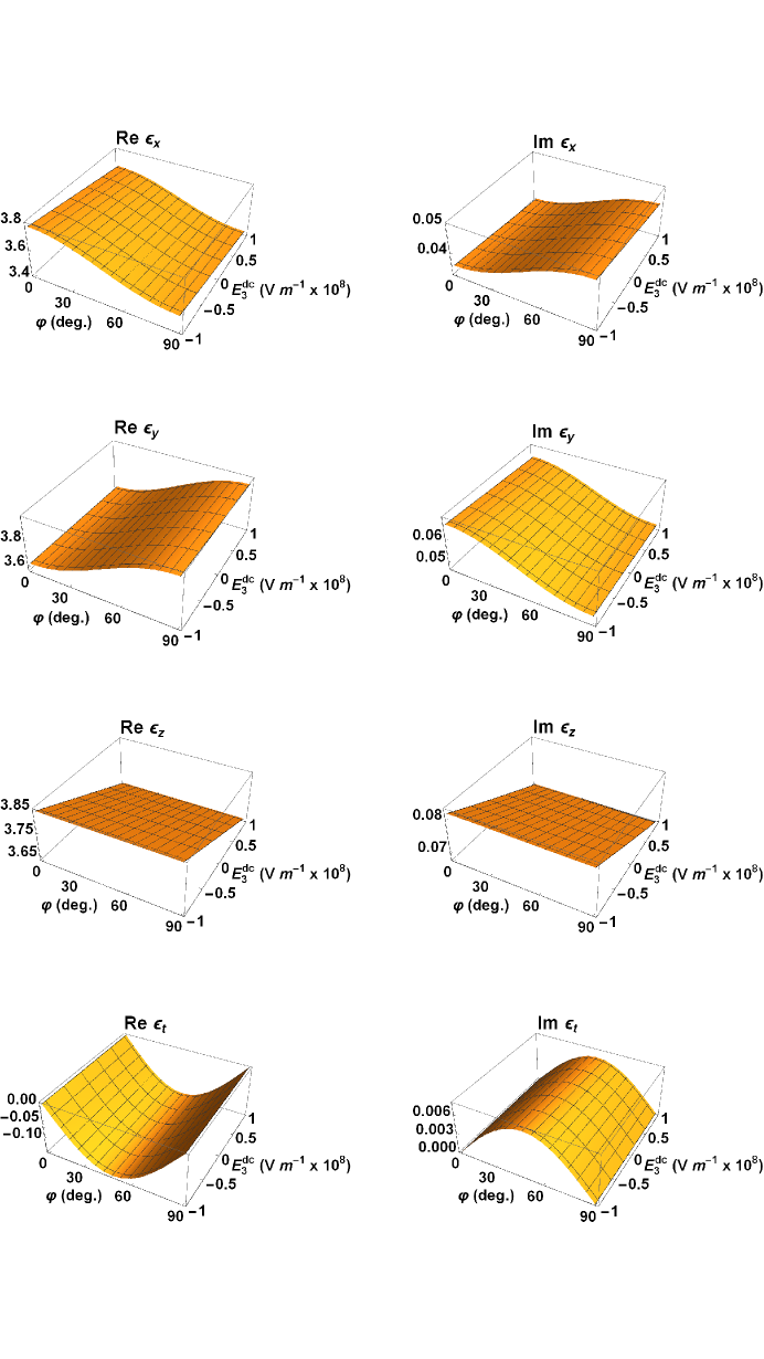
Figure 1: The extended Bruggeman estimates of relative permittivity parameters of the HCM plotted versus $E^{dc}_{3}\in\left(-1,1\right)\times 10^{8}$ $\mbox{V}\mbox{m}^{-1}$ and spheroid orientation angle $\varphi\in\left(0,90\right)^{\circ}$. The refractive index $n_{a}=1.1$, volume fraction $f_{a}=0.3$, size parameter $\eta=0.3/k_{\scriptscriptstyle 0}$, and eccentricity parameter $\rho=3$.

In Fig. 1 the real and imaginary parts of the extended Bruggeman estimates of the relative permittivity parameters $\epsilon_{x,y,z,t}$ are plotted versus the dc electric field component $E^{dc}_{3}$, and the spheroid orientation angle $\varphi$. For these calculations, the volume faction $f_{a}=0.3$, the refractive index $n_{a}=1.1$, the size parameter $\eta=0.3/k_{\scriptscriptstyle 0}$, and the eccentricity parameter $\rho=3$. We see that both the real and imaginary parts of $\epsilon_{x,y,z}$ decrease in an approximately linear manner as $E^{dc}_{3}$ increases from $-1\times 10^{8}$ $\mbox{V}\mbox{m}^{-1}$ to $1\times 10^{8}$ $\mbox{V}\mbox{m}^{-1}$, albeit this effect is much more obvious for $\epsilon_{z}$ than it is for $\epsilon_{x,y}$. The effect of $E^{dc}_{3}$ on both the real and imaginary parts of $\epsilon_{t}$ is barely discernable in Fig. 1. Both the real and imaginary parts of $\epsilon_{x,y}$ vary markedly as $\varphi$ increases from $0^{\circ}$ to $90^{\circ}$. However, the relative permittivity parameter $\epsilon_{z}$ seems to be largely unaffected by the rotation in the $xy$ plane represented by $\varphi$. The off-diagonal relative permittivity parameter $\epsilon_{t}=0$ at $\varphi=0^{\circ}$ and $90^{\circ}$; both the real and imaginary parts of $\epsilon_{t}$ increase and then decrease markedly as $\varphi$ increases from $0^{\circ}$ to $90^{\circ}$.

In addition to the dc electric field and the orientation of the component spheroids, the electromagnetic properties of HCM are also sensitive to the shapes and sizes of the component spheroids, the volume fraction, and the constitutive parameters of the component materials. These matters have been explored using the extended Bruggeman homogenization formalism in earlier studies, to which the reader is referred for further details [25, 26].

4.3 Electrical control over directions that support Voigt wave propagation

Now we investigate the effects of a dc electric field on the directions which support Voigt wave propagation in the HCM. These Voigt wave directions are represented by the Euler angles $\alpha$, $\beta$, and $\gamma$ for which $Y(\alpha,\beta,\gamma)=0$ and $W(\alpha,\beta,\gamma)\neq 0$. Notice that the angular coordinate $\gamma$ may be eliminated from our investigations since Voigt wave propagation parallel to the $z$ axis (in the rotated coordinate system) is independent of rotation about that axis. For the HCM specified by a permittivity dyadic of the form given in Eq. (14), there are generally two distinct orientations for which the Voigt wave conditions $Y=0$ and $W\neq 0$ are satisfied. We label these two orientations with the angular coordinates $\alpha=\alpha_{1,2}$ and $\beta=\beta_{1,2}$; the corresponding values of the quantity $W$ are written as $W_{1,2}$.

4.3.1 Orientation of component spheroids

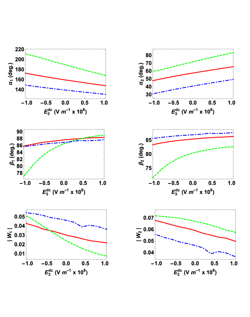
Figure 2: The angles $\alpha_{1,2}$ and $\beta_{1,2}$, along with the quantities $|W_{1,2}|$, plotted versus $E^{dc}_{3}\in\left(-1,1\right)\times 10^{8}$ $\mbox{V}\mbox{m}^{-1}$ for the spheroid orientation angles $\varphi=60^{\circ}$ (red, solid curves), $30^{\circ}$ (green, dashed curves), and $90^{\circ}$ (blue, broken dashed curves). The refractive index $n_{a}=1.1$, volume fraction $f_{a}=0.3$, size parameter $\eta=0.3/k_{\scriptscriptstyle 0}$, and eccentricity parameter $\rho=3$.

We begin by considering the effect of the dc electric field on the Voigt wave directions in relation to the orientation of the component spheroids. In Fig. 2, the angles $\alpha_{1,2}$ and $\beta_{1,2}$ along with the quantities $|W_{1,2}|$ are plotted versus $E^{dc}_{3}$ for three different orientations of the component material $a$ spheroids as given by $\varphi=30^{\circ}$ (green, dashed curves), $60^{\circ}$ (red, solid curves), and $90^{\circ}$ (blue, broken dashed curves). Here the refractive index $n_{a}=1.1$, the volume fraction $f_{a}=0.3$, the size parameter $\eta=0.3/k_{\scriptscriptstyle 0}$ and the eccentricity parameter $\rho=3$. Clearly the directions that support Voigt wave propagation are highly sensitive to the dc electric field, for all orientations of the component material $a$ spheroids considered. Specifically, the $\alpha$ angular coordinate varies by as much as $38^{\circ}$, and the $\beta$ angular coordinate varies by as much as $12^{\circ}$, as the value of $E^{dc}_{3}$ ranges from $-1\times 10^{8}$ $\mbox{V}\mbox{m}^{-1}$ to $1\times 10^{8}$ $\mbox{V}\mbox{m}^{-1}$. Generally, greater changes in the Voigt wave directions are observed for smaller values of the spheroid orientation angle $\varphi$. Also, the angular coordinate $\beta$ varies relatively little for $E^{dc}_{3}\in\left(0,1\right)\times 10^{8}$ $\mbox{V}\mbox{m}^{-1}$, but varies considerably more for $E^{dc}_{3}\in\left(-1,0\right)\times 10^{8}$ $\mbox{V}\mbox{m}^{-1}$. We note that the quantities $|W_{1,2}|$ are nonzero for all calculations, in accordance with requirements for Voigt wave propagation. Other than being nonzero, the quantities $|W_{1,2}|$ are of no obvious physical significance; therefore, plots of these quantities shall be omitted henceforth.

4.3.2 Shape of component spheroids

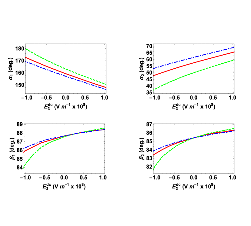
Figure 3: The angles $\alpha_{1,2}$ and $\beta_{1,2}$ plotted versus $E^{dc}_{3}\in\left(-1,1\right)\times 10^{8}$ $\mbox{V}\mbox{m}^{-1}$ for the eccentricity parameter values $\rho=3$ (red, solid curves), $2$ (green, dashed curves), and $4$ (blue, broken dashed curves). The refractive index $n_{a}=1.1$, volume fraction $f_{a}=0.3$, size parameter $\eta=0.3/k_{\scriptscriptstyle 0}$, and spheroid orientation angle $\varphi=60^{\circ}$.

We repeat the calculations of §4.3.1 but now fixing the orientation of the component material $a$ spheroids at $\varphi=60^{\circ}$ and allowing the eccentricity parameter $\rho$ to vary. The results are presented in Fig. 3 where the angles $\alpha_{1,2}$ and $\beta_{1,2}$ are plotted versus $E^{dc}_{3}$ for $\rho=2$ (green, dashed curves), $3$ (red, solid curves), and $4$ (blue, broken dashed curves). The sensitivity of the Voigt wave directions to the dc electric field is significantly modulated by the degree of eccentricity of the component spheroids. Specifically, the angular coordinates $\alpha_{1,2}$ are moderately sensitive to $\rho$. While the angular coordinates $\beta_{1,2}$ are relatively insensitive to $\rho$ for $E^{dc}_{3}\in\left(0,1\right)\times 10^{8}$ $\mbox{V}\mbox{m}^{-1}$, these angles are highly sensitive to $\rho$ for $E^{dc}_{3}\in\left(-1,0\right)\times 10^{8}$ $\mbox{V}\mbox{m}^{-1}$. The influence of the shape parameter upon the sensitivity of the Voigt wave directions in relation to $E^{dc}_{3}$ appears to be greatest for the smallest value of $\rho$ considered here.

4.3.3 Size of component spheroids

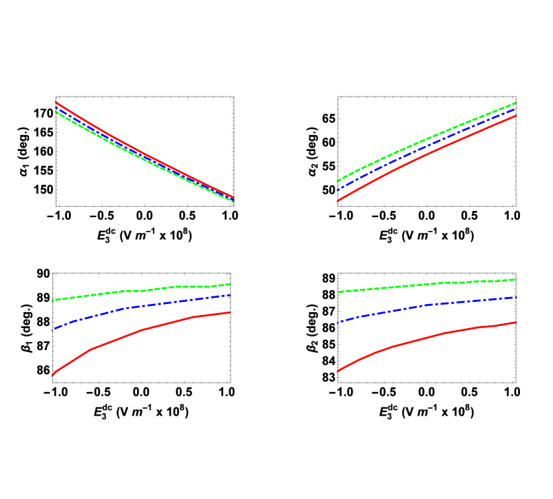
Figure 4: The angles $\alpha_{1,2}$ and $\beta_{1,2}$ plotted versus $E^{dc}_{3}\in\left(-1,1\right)\times 10^{8}$ $\mbox{V}\mbox{m}^{-1}$ for the size parameter values $\eta=0.3/k_{\scriptscriptstyle 0}$ (red, solid curves), $0.2/k_{\scriptscriptstyle 0}$ (green, dashed curves), and $0.25/k_{\scriptscriptstyle 0}$ (blue, broken dashed curves). The refractive index $n_{a}=1.1$, volume fraction $f_{a}=0.3$, spheroid orientation angle $\varphi=60^{\circ}$, and eccentricity parameter $\rho=3$.

Next we turn to the size of the component spheroids, as gauged by the size parameter $\eta$. In Fig. 4 plots similar to those in Fig. 3 are provided but here the eccentricity parameter is fixed at $\rho=3$ and three different values of size parameter are employed, namely $\eta=0.2/k_{\scriptscriptstyle 0}$ (green, dashed curves), $0.25/k_{\scriptscriptstyle 0}$ (blue, broken dashed curves), and $0.3/k_{\scriptscriptstyle 0}$ (red, solid curves). The general trends observable in Fig. 4 are similar to those observable in Fig. 3. That is, the size parameter does significantly modulate the dependency of the Voigt wave directions on the dc electric field; the influence of the size parameter is relatively modest for the $\alpha_{1,2}$ angular coordinates but is considerably stronger for the $\beta_{1,2}$ angular coordinates, especially at lower values of $E^{dc}_{3}$.

4.3.4 Volume fraction

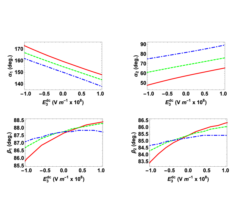
Figure 5: The angles $\alpha_{1,2}$ and $\beta_{1,2}$ plotted versus $E^{dc}_{3}\in\left(-1,1\right)\times 10^{8}$ $\mbox{V}\mbox{m}^{-1}$ for the volume fractions $f_{a}=0.3$ (red, solid curves), $0.35$ (green, dashed curves), and $0.4$ (blue, broken dashed curves). The refractive index $n_{a}=1.1$, size parameter $\eta=0.3/k_{\scriptscriptstyle 0}$, spheroid orientation angle $\varphi=60^{\circ}$, and eccentricity parameter $\rho=3$.

The influence of the volume fraction occupied by component material $a$ (or, equivalently, the porosity of component material $b$) is now considered. Plots similar to those in Fig. 4 are provided in Fig. 5 but here the size parameter $\eta=0.3/k_{\scriptscriptstyle 0}$; results are plotted for the volume fractions $f_{a}=0.3$ (red, solid curves), $0.35$ (green, dashed curves), and $0.4$ (blue, broken dashed curves). The approximate linearity of the relationship between the $\alpha_{1,2}$ angular coordinates and $E^{dc}_{3}$ is not greatly affected by the volume fraction. Furthermore, in the vicinity of $E^{dc}_{3}\approx 0\times 10^{8}$ $\mbox{V}\mbox{m}^{-1}$, the angular coordinates $\beta_{1,2}$ seem to be insensitive to the volume fraction. But for larger and smaller values of $E^{dc}_{3}$, the volume faction has a strong influence on the angular coordinates $\beta_{1,2}$ in relation to $E^{dc}_{3}$. This influence is strongest at smaller values of $f_{a}$ when $E^{dc}_{3}$ is negative–valued and at larger values of $f_{a}$ when $E^{dc}_{3}$ is positive–valued.

4.3.5 Refractive index of infiltrating fluid

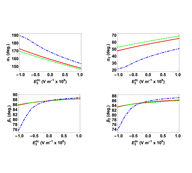
Figure 6: The angles $\alpha_{1,2}$ and $\beta_{1,2}$ plotted versus $E^{dc}_{3}\in\left(-1,1\right)\times 10^{8}$ $\mbox{V}\mbox{m}^{-1}$ for the refractive index values $n_{a}=1.1$ (red, solid curves), $1.05$ (green, dashed curves), and $1.3$ (blue, broken dashed curves). The volume fraction $f_{a}=0.3$, size parameter $\eta=0.3/k_{\scriptscriptstyle 0}$, eccentricity parameter $\rho=3$, and spheroid orientation angle $\varphi=60^{\circ}$.

Lastly, let us consider the influence of the refractive index of component material $a$, namely $n_{a}$. We repeat the calculations of Fig. 5 but with the volume fraction fixed at $f_{a}=0.3$; results are plotted in Fig. 6 for the refractive index values $n_{a}=1.05$ (green, dashed curves), $1.1$ (red, solid curves), and $1.3$ (blue, broken dashed curves). It may be seen that the refractive index strongly modulates the sensitivity of the Voigt wave directions to the dc electric field. Reminiscent of the general trends in Fig. 3, the refractive index $n_{a}$ has only a modest influence upon the angular coordinates $\beta_{1,2}$ for $E^{dc}_{3}\in\left(0,1\right)\times 10^{8}$ $\mbox{V}\mbox{m}^{-1}$, but these angles are highly sensitive to $n_{a}$ for $E^{dc}_{3}\in\left(-1,0\right)\times 10^{8}$ $\mbox{V}\mbox{m}^{-1}$. The effects of the refractive index upon the sensitivity of the Voigt wave directions in relation to $E^{dc}_{3}$ are generally greatest for the smallest value of $n_{a}$ considered here.

5 Closing comments

Voigt wave propagation has been considered for a HCM arising from a porous electro–optic host material, namely potassium niobate, infiltrated by a fluid of refractive index $n_{a}$. By means of representative numerical calculations, it has been demonstrated that the directions which support the propagation of Voigt waves may be substantially controlled by the application of a dc electric field. Furthermore, the extent to which this control may be achieved is dependent upon the porosity of the host material, the shapes, sizes and orientations of the pores, as well as the refractive index $n_{a}$.

In order to be physically realistic, the magnitude of the applied dc electric field should be less than the magnitudes of the breakdown electric fields of the materials involved. However, the breakdown electric fields depend upon the morphologies and thicknesses of the materials, with thin films generally capable of withstanding higher electric fields than bulk materials. Typical breakdown fields for potassium niobate thin films are estimated to be about $8\times 10^{7}\;\mbox{V m}^{-1}$ [27], while Kingon et al. reported no breakdown when a field of $1\times 10^{8}\;\mbox{V m}^{-1}$ was applied to a potassium niobate thin film in their experiments [28]. Accordingly, it seems reasonable here to present results for applied dc electric fields of magnitudes up to $1.0\times 10^{8}\;\mbox{V m}^{-1}$. Parenthetically, the inequality (7) is satisfied for such electric fields. In a practical device, the maximum dc electric field that could be applied may well be determined by factors other than the breakdown of the electro–optic material, such as how well the electronic components of the device can be shielded from the dc electric field. Furthermore, potassium niobate was chosen here as a representative example of an electro–optic material which has relatively large electro–optic coefficients. If artificial electro–optic materials were to be developed with larger electro–optic coefficients then this would allow the possibility of using dc electric fields of lower magnitude.

The findings reported here may be particulary significant for potential technological applications of Voigt waves. Notably, Voigt waves appear to present promising opportunities for optical sensing applications, since the directions which support Voigt wave propagation in a porous host material can be highly sensitive to changes in the refractive index of a fluid that infiltrates the host material [11]. Thus, it may be envisaged that electrical control could be harnessed to track Voigt wave propagation in an optical–sensor setting. Other possible applications of electrical control of Voigt waves may involve optical switching [29]. Such Voigt wave applications are matters for future study.

Appendix

In the extended Bruggeman formalism encapsulated by Eq. (13), the depolarization dyadics comprise the sums [30]

$$\underline{\underline{D}}_{\,\ell}=\underline{\underline{D}}^{0}_{\,\ell}+\underline{\underline{D}}^{+}_{\,\ell},\qquad(\ell=a,b).$$ (15)

The dyadic term $\underline{\underline{D}}^{0}_{\,\ell}$ represents the depolarization contribution arising in the limit $\eta\to 0$; it is given by the double integral [31, 32]

$$\underline{\underline{D}}^{0}_{\,\ell}=\frac{1}{4\pi}\,\int^{2\pi}_{\phi=0}\int^{\pi}_{\theta=0}\frac{\left(\underline{\underline{U}}^{-1}_{\,\ell}\cdot\hat{{\bf q}}\right)\,\left(\underline{\underline{U}}^{-1}_{\,\ell}\cdot\hat{{\bf q}}\right)\;\sin\theta}{\left(\underline{\underline{U}}^{-1}_{\,\ell}\cdot\hat{{\bf q}}\right)\cdot\underline{\underline{\epsilon}}_{\,HCM}\cdot\left(\underline{\underline{U}}^{-1}_{\,\ell}\cdot\hat{{\bf q}}\right)}\,d\theta\,d\phi\,,\qquad(\ell=a,b),$$ (16)

with the unit vector $\hat{{\bf q}}=\sin\theta\cos\phi\,\hat{{\bf x}}+\sin\theta\sin\phi\,\hat{{\bf y}}+\cos\theta\,\hat{{\bf z}}$. The depolarization contribution associated with the nonzero size of the component particles is represented by the dyadic term $\underline{\underline{D}}^{+}_{\,\ell}$, which is conveniently given as a 3$\times$3 subdyadic of the 6$\times$6 dyadic $\underline{\underline{\mathbb{D}}}^{+}_{\,\ell}$ per

$$\left[\,\underline{\underline{D}}^{+}_{\,\ell}\,\right]_{mn}=\left[\,\underline{\underline{\mathbb{D}}}^{+}_{\,\ell}\,\right]_{mn},\qquad\left(m,n\in\left\{1,2,3\right\}\right).$$ (17)

Here the 6$\times$6 dyadic [30]

$$\underline{\underline{\mathbb{D}}}^{+}_{\,\ell} = \frac{\omega^{4}}{4\pi\mu_{\scriptscriptstyle 0}}\int^{2\pi}_{\phi=0}\int^{\pi}_{\theta=0}\frac{\sin\theta}{\left[\left(\underline{\underline{U}}^{-1}_{\,\ell}\cdot\hat{{\bf q}}\right)\cdot\underline{\underline{\epsilon}}_{\,HCM}\cdot\left(\underline{\underline{U}}^{-1}_{\,\ell}\cdot\hat{{\bf q}}\right)\right]\left(\underline{\underline{U}}^{-1}_{\,\ell}\cdot\hat{{\bf q}}\right)\cdot\left(\underline{\underline{U}}^{-1}_{\,\ell}\cdot\hat{{\bf q}}\right)}$$

$$\times\Bigg{[}\frac{1}{\kappa_{+}-\kappa_{-}}\Bigg{(}\frac{\exp\left(i\eta q\right)}{2q^{2}}\left(1-i\eta q\right)\Big{\{}\,\mbox{det}\left[\underline{\underline{\mathbb{A}}}(\underline{\underline{U}}^{-1}_{\,\ell}\cdot{\bf q})\right]\,\underline{\underline{\mathbb{G}}}^{+}(\underline{\underline{U}}^{-1}_{\,\ell}\cdot{\bf q})$$

$$+\mbox{det}\left[\underline{\underline{\mathbb{A}}}(-\underline{\underline{U}}^{-1}_{\,\ell}\cdot{\bf q})\right]\,\underline{\underline{\mathbb{G}}}^{+}(-\underline{\underline{U}}^{-1}\cdot{\bf q})\Big{\}}\Bigg{)}^{q=\sqrt{\kappa_{+}}}_{q=\sqrt{\kappa_{-}}}+\frac{\mbox{det}\left[\underline{\underline{\mathbb{A}}}({\bf 0})\right]}{\kappa_{+}\,\kappa_{-}}\,\underline{\underline{\mathbb{G}}}^{+}({\bf 0})\Bigg{]}\;d\theta\;d\phi,\qquad(\ell=a,b),$$

with the vector ${\bf q}=q\,\hat{{\bf q}}$, the scalars $\kappa_{\pm}$ being the $q^{2}$ roots of $\mbox{det}\left[\underline{\underline{\mathbb{A}}}(\underline{\underline{U}}^{-1}\cdot{\bf q})\right]=0$, and the 6$\times$6 dyadics

$$\underline{\underline{\mathbb{A}}}({\bf p})=\left[\begin{array}[]{cc}\underline{\underline{\epsilon}}_{\,HCM}&\left({\bf p}/\omega\right)\times\underline{\underline{I}}\vspace{2mm}\\ -\left({\bf p}/\omega\right)\times\underline{\underline{I}}&\mu_{\scriptscriptstyle 0}\,\underline{\underline{I}}\end{array}\right]$$ (19)

and

$$\underline{\underline{\mathbb{G}}}^{+}({\bf p})=\underline{\underline{\mathbb{A}}}^{-1}({\bf p})-\lim_{|{\bf p}|\to\infty}\underline{\underline{\mathbb{A}}}^{-1}({\bf p}).$$ (20)

Generally, numerical methods are needed to evaluate the integrals on the right sides of Eqs. (16) and (Appendix), and also to extract the HCM permittivity dyadic $\underline{\underline{\epsilon}}_{\,HCM}$ from the nonlinear dyadic equation (13) [33].

References

- [1] M. Born and E. Wolf, Principles of Optics, 6th Edition, Pergamon Press, Oxford, UK (1980).
- [2] W. Voigt, “On the behaviour of pleochroitic crystals along directions in the neighbourhood of an optic axis,” Phil. Mag. 4, 90–97 (1902).
- [3] S. Pancharatnam, “The optical interference figures of amethystine quartz — Part II,” Proc. Ind. Acad. Sci. A 47, 210–229 (1958).
- [4] F. I. Fedorov and A. M. Goncharenko, “Propagation of light along the circular optical axes of absorbing crystals,” Opt. Spectrosc. (USSR) 14, 51–53 (1963).
- [5] G. S. Ranganath, “Optics of absorbing anisotropic media,” Curr. Sci. 67, 231–237 (1994).
- [6] T. G. Mackay and A. Lakhtakia, “Electromagnetic fields in linear bianisotropic mediums,” Prog. Optics 51, 121–209 (2008).
- [7] A. Lakhtakia, “Anomalous axial propagation in helicoidal bianisotropic media,” Opt. Commun. 157, 193–201 (1998).
- [8] M. V. Berry, “The optical singularities of bianisotropic crystals,” Proc. R. Soc. A 461, 2071–2098 (2005).
- [9] T. G. Mackay and A. Lakhtakia, “Voigt wave propagation in biaxial composite materials,” J. Opt. A: Pure Appl. Opt. 5, 91–95 (2003).
- [10] T. G. Mackay and A. Lakhtakia, “Correlation length facilitates Voigt wave propagation,” Waves Random Media 14, L1–L11 (2004).
- [11] T. G. Mackay, “On the sensitivity of directions that support Voigt wave propagation in infiltrated biaxial dielectric materials,” J. Nanophotonics 8, 083993 (2014).
- [12] T. G. Mackay, “On extended homogenization formalisms for nanocomposites,” J. Nanophotonics 2, 021850 (2008).
- [13] L. Ward, The Optical Constants of Bulk Materials and Films, 2nd edition, Institute of Physics, Bristol, UK (2000).
- [14] T. G. Mackay and A. Lakhtakia, Electromagnetic Anisotropy and Bianisotropy: A Field Guide, Word Scientific, Singapore (2010).
- [15] G. B. Arfken and H. J. Weber, Mathematical Methods for Physicists, 4th Edition, Academic Press, London, UK (1995).
- [16] J. Gerardin and A. Lakhtakia, “Conditions for Voigt wave propagation in linear, homogeneous, dielectric mediums,” Optik 112, 493–495 (2001).
- [17] R. W. Boyd, Nonlinear Optics, 2nd edition, Academic Press, San Diego, CA, USA (2003).
- [18] A. Lakhtakia and T. G. Mackay, “Electrical control of the linear optical properties of particulate composite materials,” Proc. R. Soc. A 463, 583–592 (2007).
- [19] A. Yariv and P. Yeh, Photonics: Optical Electronics in Modern Communications, 6th edition, Oxford University Press, New York, NY, USA (2007).
- [20] A. Lakhtakia, “Electrically tunable, ultranarrowband, circular–polarization rejection filters with electro–optic structurally chiral materials,” J. Eur. Opt. Soc. – Rapid Pubs. 1, 06006 (2006).
- [21] A. V. Goncharenko, “Generalizations of the Bruggeman equation and a concept of shape–distributed particle composites,” Phys. Rev. E 68, 041108 (2003).
- [22] W. S. Weiglhofer, A. Lakhtakia and B. Michel, “Maxwell Garnett and Bruggeman formalisms for a particulate composite with bianisotropic host medium,” Microwave Opt. Technol. Lett. 15, 263–266 (1997); Erratum: 22, 221 (1999).
- [23] M. Zgonik, R. Schlesser, I. Biaggio, E. Volt, J. Tscherry, and P. Günter, “Material constants of KNbO3 relevant for electro– and acousto–optics,” J. Appl. Phys. 74, 1287–1297 (1993).
- [24] T. G. Mackay and W. S. Weiglhofer, “Homogenization of biaxial composite materials: dissipative anisotropic properties,” J. Opt. A: Pure Appl. Opt. 2, 426–432 (2000).
- [25] T. G. Mackay and A. Lakhtakia, “On scattering loss in electro–optic particulate composite materials,” J. Appl. Phys. 101, 083523 (2007).
- [26] T. G. Mackay, “Voigt waves in homogenized particulate composites based on isotropic dielectric components,” J. Opt. 13, 105702 (2011).
- [27] M. J. Madou, Fundamentals of Microfabrication: The Science of Miniaturization (2nd ed), CRC Press, Boca Raton, FL (2002).
- [28] A. I. Kingon, S. H. Rou, M. S. Ameen, T. M. Graettinger, K. Gifford, and O. Auciello, “Deposition of electrooptic thin films,” Ceramic Transactions 14, Electro-Optics and Non-linear Optic Materials, (Am. Cer. Soc., Westerville, OH), 1990, pp. 179–196.
- [29] T. S. El-Bawab, Optical Switching, Springer, New York, NY, USA (2006).
- [30] T. G. Mackay, “Depolarization volume and correlation length in the homogenization of anisotropic dielectric composites,” Waves Random Media 14, 485–498 (2004); Erratum: Waves Random Complex Media 16, 85 (2006).
- [31] B. Michel, “A Fourier space approach to the pointwise singularity of an anisotropic dielectric medium,” Int. J. Appl. Electromagn. Mech. 8, 219–227 (1997).
- [32] B. Michel and W. S. Weiglhofer, “Pointwise singularity of dyadic Green function in a general bianisotropic medium,” Arch. Elekron. Übertrag. 51, 219–223 (1997); Erratum: 52, 31 (1998).
- [33] B. Michel, A. Lakhtakia and W. S. Weiglhofer, “Homogenization of linear bianisotropic particulate composite media — Numerical studies,” Int. J. Appl. Electromag. Mech. 9, 167–178 (1998); Erratum: 10, 537–538 (1999).