Abstract

Various results based on some convexity assumptions (involving the exponential map along with affine maps, geodesics and convex hulls) have been recently established on Hadamard manifolds. In this paper we prove that these conditions are mutually equivalent and they hold if and only if the Hadamard manifold is isometric to the Euclidean space. In this way, we show that some results in the literature obtained on Hadamard manifolds are actually nothing but their well known Euclidean counterparts.

Keywords: Hadamard manifold; convexity.
MSC: 53C23; 53C24.

1 Introduction

In recent years considerable efforts have been done to extend concepts and results from the Euclidean/Hilbert context to settings with no vector space structure. The motivation of such studies comes from nonlinear phenomena which require the presence of a non-positively curved structure for the ambient space; see Jost [3], Kristály [4], Kristály, Rădulescu and Varga [5], Li, López and Martín-Márquez [7], Németh [9], Udrişte [12] and references therein.

The purpose of the present paper is to point out some conceptual mistakes within the class of Hadamard manifolds where some authors used equivalences between convexity notions which basically reduce the geometric setting to the Euclidean one. Thus, in all these papers the corresponding results and their consequences are nothing but previously well known facts in the Euclidean case.

To be more precise, let $(M,g)$ be a Hadamard manifold (i.e., simply connected, complete Riemannian manifold with non-positive sectional curvature). According to the Cartan-Hadamard theorem, the exponential map $\exp_{p}:T_{p}M\to M$ is a global diffeomorphism for every $p\in M$. Let $p\in M$ be fixed arbitrarily. By using the exponential map, three convexity notions are recalled in the sequel, mentioning also their sources without sake of completeness:

• Affinity. A map $f:M\to\mathbb{R}$ is called affine if $f\circ\gamma:[0,1]\to\mathbb{R}$ is affine in the usual sense on $[0,1]$ for every geodesic segment $\gamma:[0,1]\to M.$ Papa Quiroz [10] and Papa Quiroz and Oliveira [11] claimed that $M\ni q\mapsto g_{p}(\exp_{p}^{-1}(q),y)$ is affine for every $y\in T_{p}M$ and they used this property to prove convergence of various algorithms on Hadamard manifolds. This statement is also used in Colao, López, Marino and Martín-Márquez [1], and Zhou and Huang [14].

• Geodesics. Let $q_{1},q_{2}\in M$ be two fixed points. By construction, the unique minimal geodesic $\gamma:[0,1]\to M$ joining these points is given by $\gamma(t)=\exp_{q_{1}}(t\exp_{q_{1}}^{-1}(q_{2})).$ Yang and Pu [15] claimed that the curve $[0,1]\ni t\mapsto\exp_{p}((1-t)\exp_{p}^{-1}(q_{1})+t\exp_{p}^{-1}(q_{2}))$ is also a minimal geodesic segment on $M$ joining the points $q_{1}$ and $q_{2}.$

• Convex hull. By definition (see [3, page 67]), the convex hull C$(S)$ of a set $S\subset M$ is the smallest convex subset of $M$ containing $S.$ Instead of the convex hull, Yang and Pu [15] introduced the geodesic convex hull GC${}_{p}(S)$ of a set $S\subset M$ with respect to $p\in M$ in the following way

  $${\rm GC}_{p}(S)=\left\{\exp_{p}\left(\sum_{i=1}^{m}\lambda_{i}\exp_{p}^{-1}(q_{i})\right):\ \forall q_{1},...,q_{m}\in S;\lambda_{1},...,\lambda_{m}\in[0,1],\sum_{i=1}^{m}\lambda_{i}=1\right\}.$$

  It is claimed in [15] that C$(S)={\rm GC}_{p}(S)$ for every $p\in M$ and $S\subset M.$

We provide below a concrete counterexample in the hyperbolic plane which shows that the aforementioned claims are based on a fundamental misconception.

Example 1.1

Consider the Poincaré upper half-plane model $\mathbb{H}=\{(u,v)\in\mathbb{R}^{2}:v>0\}$ endowed with the Riemannian metric defined for every $(u,v)\in\mathbb{H}$ by

$$g_{ij}(u,v)=\frac{1}{v^{2}}\delta_{ij},\quad\text{for }i,j=1,2.$$

$(\mathbb{H},g)$ is a Hadamard manifold with constant sectional curvature $-1$ and the geodesics in $\mathbb{H}$ are the semilines and the semicircles orthogonal to the line $v=0$. The Riemannian distance between two points $(u_{1},v_{1}),(u_{2},v_{2})\in\mathbb{H}$ is given by

$$d_{\mathbb{H}}\left((u_{1},v_{1}),(u_{2},v_{2})\right)={\rm arccosh}\left(1+\frac{(u_{2}-u_{1})^{2}+(v_{2}-v_{1})^{2}}{2v_{1}v_{2}}\right).$$

Fix $p=(0,1)$. By some elementary calculations (see also [12, page 20]) we have that for each $(\alpha,\beta)\in T_{p}\mathbb{H}$,

$$\exp_{p}(\alpha,\beta)=\begin{cases}(0,e^{\beta})&\mbox{if }\alpha=0\\ \left(\frac{\beta}{\alpha}+r_{\alpha,\beta}\tanh(s_{\alpha,\beta}),\frac{r_{\alpha,\beta}}{\cosh(s_{\alpha,\beta})}\right)&\mbox{if }\alpha\neq 0,\end{cases}$$

where $r_{\alpha,\beta}=\sqrt{1+\left(\frac{\beta}{\alpha}\right)^{2}}$ and

$$s_{\alpha,\beta}=\begin{cases}\sqrt{\alpha^{2}+\beta^{2}}-{\rm arcsinh}\frac{\beta}{\alpha}&\mbox{if }\alpha>0\\ -\sqrt{\alpha^{2}+\beta^{2}}-{\rm arcsinh}\frac{\beta}{\alpha}&\mbox{if }\alpha<0.\end{cases}$$

In other words, $\exp_{p}(\alpha,\beta)$ belongs to the semiline $\{u=0,v>0\}$ or a semicircle orthogonal to the line $v=0$ that contains $p$ and for which the direction of the tangent in $p$ is given by the vector $(\alpha,\beta)$. Moreover, $d_{\mathbb{H}}\left(p,\exp_{p}(\alpha,\beta)\right)=\|(\alpha,\beta)\|=\sqrt{\alpha^{2}+\beta^{2}}$.

Let $q_{1}=\left(1,\sqrt{2}\right)$, $q_{2}=\left(-1,\sqrt{2}\right)$ and take $S=\{q_{1},q_{2}\}$. Then,

$${\rm C}(S)=\{(u,v)\in\mathbb{R}^{2}:u^{2}+v^{2}=3,u\in[-1,1],v>0\}.$$

The geodesic segment joining $p$ and $q_{1}$ belongs to the semicircle $K=\{(u,v)\in\mathbb{R}^{2}:(u-1)^{2}+v^{2}=2,v>0\}$. Denote $\eta_{1}=\exp_{p}^{-1}(q_{1})=(\alpha,\alpha)$ and $\eta_{2}=\exp_{p}^{-1}(q_{2})=(-\alpha,\alpha)$ with $\alpha=\ln(\sqrt{2}+1)^{1/\sqrt{2}}$ (see also [13, Section 5] for the general expression of the inverse exponential map).

Let $\eta=(1/2)\eta_{1}+(1/2)\eta_{2}=(0,\alpha)$ and $(0,x)=\exp_{p}(\eta)$. Then $x=(\sqrt{2}+1)^{1/\sqrt{2}}>\sqrt{3}$. Thus,

$${\rm C}(S)\neq{\rm GC}_{p}(S).$$

Actually, since $(1-t)\eta_{1}+t\eta_{2}=\left((1-2t)\alpha,\alpha\right)$, the set ${\rm GC}_{p}(S)$ consists of the points $\exp_{p}\left((1-2t)\alpha,\alpha\right)$, with $t\in[0,1]$, see Figure 1.

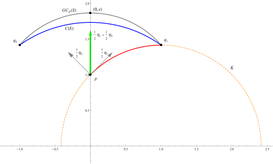
Figure 1: Difference between convex hull and geodesic convex hull.

Note that the above fact also shows that the curve $[0,1]\ni t\mapsto\exp_{p}((1-t)\exp_{p}^{-1}(q_{1})+t\exp_{p}^{-1}(q_{2}))$ is not the minimal geodesic joining $q_{1}$ and $q_{2}$.

It is well known that any affine mapping defined on $\mathbb{H}$ is constant. In particular, one can choose $y\in T_{p}\mathbb{H}\setminus\{0\}$ such that the mapping $\mathbb{H}\ni q\mapsto\langle\exp_{p}^{-1}(q),y\rangle$ is not constant and so it is not affine. This fact can be checked directly as well. Moreover, it is also obvious that $\exp_{p}:T_{p}\mathbb{H}\to\mathbb{H}$ is not a global isometry.

2 Main result

As the main result of this paper we prove the following rigidity theorem.

Theorem 2.1

Let $(M,g)$ be an $n-$dimensional Hadamard manifold and $p\in M.$ Then the following statements are equivalent:

• The map $M\ni q\mapsto g_{p}(\exp_{p}^{-1}(q),y)$ is affine for every $y\in T_{p}M;$

• For every $q_{1},q_{2}\in M$, the curve $[0,1]\ni t\mapsto\exp_{p}((1-t)\exp_{p}^{-1}(q_{1})+t\exp_{p}^{-1}(q_{2}))$ is the minimal geodesic segment joining the points $q_{1}$ and $q_{2};$

• For every non-empty set $S\subset M$, C$(S)={\rm GC}_{p}(S);$

• The map $\exp_{p}:T_{p}M\to M$ is a global isometry;

• The sectional curvature on $(M,g)$ is identically zero $($i.e., $(M,g)$ is isometric to the usual Euclidean space $(\mathbb{R}^{n},e)).$

In order to prove Theorem 2.1, we recall two results.

Proposition 2.1

[Choquet theorem; see [12, Theorem 6.5]] An $n-$dimensional Riemannian manifold $(M,g)$ is the Riemannian product of an $(n-p+1)-$dimensional Riemannian manifold and the Euclidean space $\mathbb{R}^{p-1}$ $($at least locally$)$ if and only if the vector space of all affine functions on $M$ has dimension $p.$ $[$In particular, the sectional curvature restricted to the components of $\mathbb{R}^{p-1}$ is identically zero.$]$

Proposition 2.2

[See [3, Lemma 3.3.1]] The convex hull C$(S)$ of a set $S\subset M$ is

$${\rm C}(S)=\bigcup_{k=0}^{\infty}S_{k},$$

where $S_{0}=S$ and for every $k\in\mathbb{N}$, $S_{k}$ is the union of all geodesic segments between points of $S_{k-1}.$

Now, we are ready to prove our rigidity result.

Proof of Theorem 2.1. The equivalence (iv)$\Leftrightarrow$(v) is trivial, see [2, Theorem 4.1].

(v)$\Rightarrow$(ii) This implication follows directly because property (ii) is satisfied in the Euclidean space $(\mathbb{R}^{n},e)$ and geodesics are invariant by isometries between Hadamard manifolds.

(ii)$\Rightarrow$(iii) is also trivial, coming from the two definitions and elementary computations.

(ii)$\Rightarrow$(i) Let $y\in T_{p}M$ be fixed arbitrarily; for convenience, let $f_{y}:M\to\mathbb{R}$ be defined by $f_{y}(q)=g_{p}(\exp_{p}^{-1}(q),y)$. By assumption, any geodesic segment in $M$ can be represented by $\gamma=\exp_{p}\circ\gamma_{0}$, where $\gamma_{0}(t)=(1-t)\exp_{p}^{-1}(q_{1})+t\exp_{p}^{-1}(q_{2})$, $t\in[0,1]$ for some $q_{1},q_{2}\in M.$ Then,

$$f_{y}(\gamma(t))=g_{p}(\exp_{p}^{-1}(\gamma(t)),y)=g_{p}(\gamma_{0}(t),y)=(1-t)g_{p}(\exp_{p}^{-1}(q_{1}),y)+tg_{p}(\exp_{p}^{-1}(q_{2}),y),$$

which is an affine function on $[0,1]$ in the usual sense.

(i)$\Rightarrow$(v) We show that the dimension of the space of affine functions on $M$ is $n+1.$ By assumption, $f_{y}(q)=g_{p}(\exp_{p}^{-1}(q),y)$ is an affine function on $M$ for every $y\in T_{p}M$. In particular, it follows that ${\rm Hess}_{g}f_{y}=0,$ since $f_{y}$ is both convex and concave, see [12]. Since Hess${}_{g}f_{y}(V,W)=g(\nabla_{V}{\rm grad}f_{y},W)$ for every vector fields $V,W$ on $M$, the latter relation implies in particular that grad$f_{y}$ is a parallel vector field along any geodesic of $M$. Since dim$(M)=n$, we may fix $y_{1},...,y_{n}\in T_{p}M$ such that in every $q\in M$, the set $\{{\rm grad}f_{y_{1}},...,{\rm grad}f_{y_{n}}\}$ forms a basis of the tangent space $T_{q}M$ (basically, it is enough to guarantee this property just in one point and use parallel transport at any fixed point). In this manner, we constructed exactly $n$ non-constant, linearly independent affine functions $f_{y_{i}}$ on $M$, $i=1,...n,$ corresponding to the elements $y_{1},...,y_{n}\in T_{p}M$. Moreover, we may add to this set also a constant function which is affine and linearly independent of $\{f_{y_{1}},...,f_{y_{n}}\}.$ Therefore, the vector space of all affine functions on $M$ has dimensional $p\geq n+1$. According to Choquet theorem (see Proposition 2.1), we also have that $p\leq n+1$. Therefore, $p=n+1$ and again by Choquet theorem and from the fact that $(M,g)$ is a Hadamard manifold, it follows that $M$ is globally represented as $\mathbb{R}^{n}$ whose sectional curvature is identically zero.

(iii)$\Rightarrow$(ii) Let $q_{1},q_{2}\in M$ and $S=\{q_{1},q_{2}\}$. On the one hand, by the definition of the geodesic convex hull, since $S$ contains just two elements, we clearly have that

$$\text{GC}_{p}(S) = \left\{\exp_{p}\left(\lambda_{1}\exp_{p}^{-1}(q_{1})+\lambda_{2}\exp_{p}^{-1}(q_{2})\right):\lambda_{1},\lambda_{2}\in[0,1],\ \lambda_{1}+\lambda_{2}=1\right\}$$

$$= \left\{\exp_{p}\left((1-t)\exp_{p}^{-1}(q_{1})+t\exp_{p}^{-1}(q_{2})\right):t\in[0,1]\right\}.$$

On the other hand, if $S_{0}=S$, then the set $S_{1}$ in Proposition 2.2 is precisely the image of the unique minimal geodesic segment $\gamma:[0,1]\to M$ joining the points $q_{1}$ and $q_{2}$. Moreover, if we take any two points in $S_{1}={\rm Im}(\gamma)$ and join them by a geodesic segment, the minimality of $\gamma$ implies that the image of the latter geodesic will be a subset of ${\rm Im}(\gamma)$. Therefore, $S_{1}=S_{2}=...={\rm Im}(\gamma)$. Consequently, ${\rm C}(S)={\rm Im}(\gamma).$ Since by assumption ${\rm C}(S)=\text{GC}_{p}(S),$ one obtains (ii). $\square$

Remark 2.1

Further definitions and open questions concerning the convex hull on non-positively curved spaces can be found in the literature, see Ledyaev, Treiman and Zhu [6, Conjecture 1] and Nava-Yazdani and Polthier [8]. It would be interesting to study the relationship between these notions and the geometric structure of the ambient space.

Acknowledgment. A. Kristály was supported by a grant of the Romanian Ministry of Education, CNCS-UEFISCDI, project number PN-II-RU-TE-2011-3-0047. C. Li and G. López were supported by DGES (Grant MTM2012-34847-C02-01). A. Nicolae was supported by a grant of the Romanian Ministry of Education, CNCS-UEFISCDI, project number PN-II-RU-PD-2012-3-0152. Part of this work was carried out while some of the authors were visiting the University of Seville supported by DGES (Grant MTM2012-34847-C02-01).

References

- [1] V. Colao, G. López, G. Marino, V. Martín-Márquez, Equilibrium problems in Hadamard manifolds. J. Math. Anal. Appl. 388 (2012), no. 1, 61–77.
- [2] M. P. do Carmo, Riemannian Geometry, Birkhäuser, Boston, 1992.
- [3] J. Jost, Nonpositive Curvature: Geometric and Analytic Aspects. Birkhäuser Verlag, Basel, 1997.
- [4] A. Kristály, Nash-type equilibria on Riemannian manifolds: a variational approach. J. Math. Pures Appl. (9) 101 (2014), no. 5, 660–688.
- [5] A. Kristály, V. Rădulescu, Cs. Varga, Variational Principles in Mathematical Physics, Geometry, and Economics, Cambridge University Press, Encyclopedia of Mathematics and its Applications, No. 136, Cambridge, 2010.
- [6] Y. S. Ledyaev, J. S. Treiman, Q. J. Zhu, Helly’s intersection theorem on manifolds of nonpositive curvature. J. Convex Anal. 13 (2006), no. 3-4, 785–798.
- [7] C. Li, G. López, V. Martín-Márquez, Monotone vector fields and the proximal point algorithm on Hadamard manifolds. J. Lond. Math. Soc. (2) 79 (2009), no. 3, 663–683.
- [8] E. Nava-Yazdani, K. Polthier, De Casteljau’s algorithm on manifolds. Comp. Aided Geom. Design 30(2013), 722–732.
- [9] S. Z. Németh, Variational inequalities on Hadamard manifolds. Nonlinear Anal. 52 (2003), 1491–1498.
- [10] E. A. Papa Quiroz, An extension of the proximal point algorithm with Bregman distances on Hadamard manifolds. J. Global Optim. 56 (2013), no. 1, 43–59.
- [11] E. A. Papa Quiroz, P. R. Oliveira, Proximal point methods for quasiconvex and convex functions with Bregman distances on Hadamard manifolds. J. Convex Anal. 16 (2009), no. 1, 49–69.
- [12] C. Udrişte, Convex Functions and Optimization Methods on Riemannian Manifolds, Mathematics and its Applications, 297. Kluwer Academic Publishers Group, Dordrecht, 1994.
- [13] X. Wang, C. Li, J.-C. Yao, Projection algorithms for solving convex feasibility problems on Hadamard manifolds. J. Nonlinear Convex Anal., in press.
- [14] L.-W. Zhou, N.-J. Huang, Existence of solutions for vector optimization on Hadamard manifolds. J. Optim. Theory Appl. 157 (2013), no. 1, 44–53.
- [15] Z. Yang, Y. J. Pu, Existence and stability of solutions for maximal element theorem on Hadamard manifolds with applications. Nonlinear Anal. 75 (2012), no. 2, 516–525.