Recovering of dielectric constants of explosives via a globally strictly convex cost functional

Abstract

The inverse problem of estimating dielectric constants of explosives using boundary measurements of one component of the scattered electric field is addressed. It is formulated as a coefficient inverse problem for a hyperbolic differential equation. After applying the Laplace transform, a new cost functional is constructed and a variational problem is formulated. The key feature of this functional is the presence of the Carleman Weight Function for the Laplacian. The strict convexity of this functional on a bounded set in a Hilbert space of an arbitrary size is proven. This allows for establishing the global convergence of the gradient descent method. Some results of numerical experiments are presented.

Keywords: Coefficient inverse problem, Laplace transform, Carleman weight function, strictly convex cost functional, global convergence, Laguerre functions, numerical experiments.

AMS classification codes: 35R30, 35L05, 78A46

1 Introduction

The detection and identification of explosive devices has always been of particular interest to security and mine-countermeasures. One of the most popular techniques used for the purpose of detection and identification is the Ground Penetrating Radar (GPR). Exploiting the energy of backscattering electromagnetic pulses measured on a boundary, the GPR allows for mapping the internal structures containing explosives. Although this concept is not new, combining the GPR with quantitative imaging may significantly enhance the detection and especially identification of explosive devices. This idea was recently proposed and developed in a series of publications. For example, we mention [3, 5, 9, 10], where three-dimensional (3-d) quantitative imaging of dielectric constants of targets mimicking explosives was performed using experimental backscattering measurements; we also refer to [7] for 1-d imaging using real data collected in the field by a Forward Looking Radar.

In the above works, the imaging problem was formulated as a Coefficient Inverse Problem (CIP) for a time dependent wave-like PDE. The main question in performing quantitative imaging is as follows: How to find a good approximation of the solution to the corresponding CIP without any advanced knowledge of a small neighborhood of this solution? We call a numerical method providing such an approximation globally convergent. As soon as this approximation is found, a number of conventional locally convergent methods may be used to refine that approximation, see, e.g., Chapters 4 and 5 of [3] for a two-stage numerical procedure.

It is well known that the objective functionals resulted from applying the traditional least-squares method are usually nonconvex. This fact explains existence of multiple local minima and ravines of those functionals. In turn, the latter leads to the local convergence of gradient and Newton-like methods. That is, the convergence of these methods is guaranteed only if an initial approximation lies in a small neighborhood of the solution. However, from our experience working with experimental data (see above citations), we have observed that such a requirement is not normally satisfied in practical situations.

In this paper we propose a new numerical method which provides the global convergence. Currently there are two approaches to constructing globally convergent algorithms. They were developed in a number of publications summarized in books [3, 8]. In particular, the above cited works treating experimental data use the approach of [3]. The common part of both approaches is the temporal Laplace transform. Let $s>0$ be the parameter in the Laplace transform. We assume that $s\geq\underline{s}$, where $\underline{s}$ is a large enough positive constant. Then, applying the Laplace transform to the time-dependent wave-like PDE, one obtains a boundary value problem for a nonlinear integral differential equation. However, the main difficulty then is that the integration over the parameter $s$ is required on the infinite interval $\left(s,\infty\right)$. In the convexification method [8] that integral was truncated, and the residual was set to zero. Unlike this, in [3] the residual, i.e., the so-called “tail function”, was approximated in an iterative process.

The open question is whether it is possible to avoid such a truncation. In other words, whether it is possible to avoid a procedure of approximating the tail function. This question is addressed in the current paper.

The main novelty here is that the truncation of the infinite integral is replaced by the truncation of a series with respect to some $s$-dependent functions forming an orthonormal basis in $L_{2}\left(\underline{s},\infty\right).$ In this way, we obtain a coupled system of nonlinear elliptic equations with respect to the $x-$dependent coefficients of the truncated series, where $x\in\mathbb{R}^{3}$. In addition, we construct a least squares objective functional with a Carleman Weight Function (CWF) in it. The main result is formulated in Theorem 4.2. Given a bounded set of an arbitrary size in a certain Hilbert space, one can choose a parameter of the CWF such that this functional becomes strictly convex on this set. This implies convergence of gradient methods in finding the unique minimizer of the functional on that set, if it exists, starting from any point of that set. Since restrictions on the diameter of that bounded set are not imposed, we call the latter global convergence and we call that functional globally strictly convex. This idea also works in the case when the Fourier transform is applied to the wave-like equation instead of the Laplace transform.

To demonstrate the computational feasibility of the proposed method, we perform a limited numerical study in the 1-d case. In particular, we show numerically that if a locally convergent algorithm starts from an approximation obtained by the proposed globally convergent algorithm, then the accuracy of approximations can be significantly improved. On the other hand, if that locally convergent algorithm starts from the background medium, then it may fail to perform well. In section 2 we formulate our inverse problem and theorems in 3-d. In sections 3–5 we prove these theorems. In section 6 we briefly summarize the special case of the 1-d problem. Section 7 describes some details of the numerical implementation in the 1-d case. Finally, in section 8 we demonstrate the numerical performance of the proposed algorithm.

2 The 3-d coefficient inverse problem

Below $x=\left(x_{1},x_{2},x_{3}\right)\in\mathbb{R}^{3}.$ Let $\Omega\subset\mathbb{R}^{3}$ be a convex bounded domain with a piecewise-smooth boundary $\partial\Omega$. We define $S_{\infty}:=\partial\Omega\times\left(0,\infty\right).$ Let the function $c\left(x\right)$ satisfies the following conditions

$$c\in C^{1+\alpha}\left(\mathbb{R}^{3}\right),\ c_{0}\leq c\left(x\right)\leq 1+d,\forall x\in\mathbb{R}^{3},\ c\left(x\right)=1,\ x\in\mathbb{R}^{3}\diagdown\Omega,$$ (1)

where the numbers $c_{0}\in\left(0,1\right)$ and $d>0$ are given. In this paper, $C^{m+\alpha}$ denotes Hölder spaces, where $m\geq 0$ is an integer and $\alpha\in\left(0,1\right)$. Consider the following Cauchy problem

$$c\left(x\right)u_{tt}=\Delta u\left(x,t\right)+\delta(x_{3}-x_{3}^{0})f(t),\left(x,t\right)\in\mathbb{R}^{3}\times\left(0,\infty\right),$$ (2)

$$u\left(x,0\right)=0,u_{t}\left(x,0\right)=0.$$ (3)

The coefficient $c\left(x\right)$ represents the spatially distributed dielectric constant. Here $c(x)$ is normalized so that its value in the background medium, i.e., in $\mathbb{R}^{3}\setminus\Omega$, equals $1$. The function $u\left(x,t\right)$ represents one of components of the electric field generated by an incident plane wave propagating along the $x_{3}-$axis and excited at the plane $\left\{x_{3}=x_{3}^{0}\right\},$ where $x_{3}^{0}\notin\overline{\Omega}$. The function $f\left(t\right)\not\equiv 0$ is continuous and bounded which represents the time-dependent waveform of the incident plane wave. Of course, the propagation of electromagnetic waves should be modeled by the Maxwell’s equations. However, there are two reasons for us to use the scalar equation (2). The first reason is that most GPR systems provide only scalar data instead of three components of the electric field. For example, in the experiments used in [3, 5, 7, 9, 10] only one component of the electric field was generated by the source and the detector measured only that component of the backscattering electric field. The second reason is that it was demonstrated numerically in [4] that if the incident wave has only one non-zero component of the electric field, then this component dominates the other two. Moreover, equation (2) approximates well the propagation of that component even in 3-d [4].

CIP 1: Suppose that conditions (1)–(3) are satisfied and that the plane $\left\{x_{3}=x_{3}^{0}\right\}\subset\left(\mathbb{R}^{3}\setminus\overline{\Omega}\right)$. Determine the coefficient $c(x)$ for $x\in\Omega,$ assuming that the following function $p_{1}(x,t)$ is known

$$u|_{S_{\infty}}=p_{1}(x,t).$$ (4)

The function $p_{1}(x,t)$ in (4) models a boundary measurement. Having $p_{1}(x,t)$, one can uniquely solve the initial value problem (2)–(3) outside of the domain $\Omega.$ Hence, the normal derivative is also known:

$$\partial_{n}u\mid_{S_{\infty}}=p_{2}\left(x,t\right).$$ (5)

We note that the knowledge of functions $p_{1}(x,t)$ and $p_{2}\left(x,t\right)$ on an infinite rather than finite time interval is not a serious restriction of our method, since the Laplace transform, which we use, effectively cuts off values of these functions for large $t$. In addition, if the incident plane wave is excited on a finite time interval, the scattered wave will eventually vanish, as we observed in our experiments in [3, 5, 7, 9, 10]. In practice, incident waves are usually excited for a short period of time.

3 The coupled system of nonlinear elliptic equations

Consider the Laplace transform $\tilde{u}(x,s):=\left(\mathcal{L}u\right)\left(x,s\right)=\int_{0}^{\infty}u\left(x,t\right)e^{-st}dt,\ s>0,$ where $s$ is referred to as the pseudofrequency. We also denote by $\tilde{f}(s)=\left(\mathcal{L}f\right)(s)$ the Laplace transform of $f(t)$. Consider $s\geq\underline{s}(d)>0$, where the number $\underline{s}\left(d\right)$ is large enough, so that the Laplace transforms of $u$ and its derivatives $D^{\beta}u,\left|\beta\right|=1,2,$ converge absolutely. The number $d$ is defined in (1). We assume that $\tilde{f}(s)\neq 0$ for all $s\geq\underline{s}(d)$. Define $w(x,s):=\tilde{u}(x,s)/\tilde{f}(s)$. Then, this function satisfies the equation:

$$\Delta w(x,s)-s^{2}c(x)w(x,s)=-\delta(x_{3}-x_{3}^{0}),\ x\in\mathbb{R}^{3},\ s\geq\underline{s}\left(d\right).$$ (6)

Define $w_{0}\left(x_{3},s\right):=e^{-s|x_{3}-x_{3}^{0}|}/(2s).$ Note that $w_{0}(x_{3},s)$ tends to zero as $\left|x_{3}\right|\rightarrow\infty.$ The function $w_{0}\left(x_{3},s\right)$ is the unique solution of equation (6) in the case $c(x)\equiv 1$ which tends to zero as $\left|x_{3}\right|\rightarrow\infty.$ It is shown in Theorem 3.1 of [10] that in the case $f\left(t\right)=\delta\left(t\right)$

$$\lim_{\left|x\right|\rightarrow\infty}\left[w\left(x,s\right)-w_{0}(x_{3},s)\right]=0$$ (7)

and that the function $w\left(x,s\right)$ can be represented in the form

$$w\left(x,s\right)=w_{0}\left(x_{3},s\right)+\widehat{w}\left(x,s\right),\text{ where }\widehat{w}\left(x,s\right)\in C^{2+\alpha}\left(\mathbb{R}^{3}\right),\ \forall s\geq\underline{s}\left(d\right).$$ (8)

Furthermore, the same theorem claims that $w(x,s)>0$ for all $s>\underline{s}\left(d\right)$. Thus, we assume these properties in our algorithm even if $f\left(t\right)\neq\delta\left(t\right).$ Next, define $v:=(\ln w)/s^{2}$. Substituting $w=e^{vs^{2}}$ into (6) and keeping in mind that $\overline{\Omega}\cap\{x_{3}=x_{3}^{0}\}=\varnothing$, we obtain

$$\Delta v+s^{2}|\nabla v|^{2}=c(x),x\in\Omega.$$ (9)

Hence, if the function $v$ is known, then the coefficient $c(x)$ can be computed directly using (9). We define $q:=\partial v/\partial s$. Thus, $v\left(x,s\right)=-\int\limits_{s}^{\infty}q\left(x,\tau\right)d\tau.$ Note that this converges absolutely together with its derivatives with respect to $x$ up to the second order. The latter is true if certain non-restrictive conditions are imposed on the function $c\left(x\right)$ (see Lemma 6.5.2 in [8]), and we assume that these conditions are in place. Hence, differentiating (9) with respect to $s$ leads to the following nonlinear integral differential equation as mentioned in Introduction:

$$\Delta q-2s^{2}\nabla q\int\limits_{s}^{\infty}\nabla q\left(x,\tau\right)d\tau+2s\big{(}\int\limits_{s}^{\infty}\nabla q\left(x,\tau\right)d\tau\big{)}^{2}=0,x\in\Omega,s\geq\underline{s}\left(d\right).$$ (10)

In addition, the following two boundary functions $\varphi\left(x,s\right)$, $\psi\left(x,s\right)$ can be derived from functions $p_{1}\left(x,t\right)$, $p_{2}\left(x,t\right)$ in (4) and (5)

$$q\mid_{\partial\Omega}=\phi\left(x,s\right),\quad\partial_{n}q\mid_{\partial\Omega}=\psi\left(x,s\right),\ s\geq\underline{s}\left(d\right).$$ (11)

We have obtained the nonlinear boundary value problem (10)–(11) for $q\left(x,s\right).$ If this function is found, then the coefficient $c\left(x\right)$ can be easily found via backwards calculations. Therefore, the central focus should be on the solution of the problem (10)–(11).

We remark that functions $p_{1}\left(x,t\right),p_{2}\left(x,t\right)$ are results of measurements. Hence, they contain noise. Although one needs to calculate the first derivative with respect to $s$ of functions $\left(\mathcal{L}p_{1}\right)\left(x,s\right)$, $\left(\mathcal{L}p_{2}\right)\left(x,s\right)$ in order to find functions $\phi\left(x,s\right)$, $\psi\left(x,s\right),$ it was observed in [3] that this can be done in a stable way, since the Laplace transform smooth out the that noise. In addition, in our numerical computation we also remove high frequency noise by truncating high order Fourier coefficients in the Fourier transformed data.

There have been two globally convergent method proposed by our group so far [3, 8]. The common point of both methods is that the integral in (10) is written as

$$\int\limits_{s}^{\infty}\nabla q(x,\tau)d\tau=\int\limits_{s}^{\bar{s}}\nabla q(x,\tau)d\tau+\nabla V(x,\bar{s}),\text{ }\nabla V(x,\bar{s})=\int\limits_{\bar{s}}^{\infty}\nabla q(x,\tau)d\tau.$$

The function $V$ is called the “tail function”. In the method of [8] this tail function was set to be zero, whereas in [3] it was approximated in an iterative process.

The key novelty of the method of this paper is that it does not truncate the integral over $s$ in (10) as in the above methods. Instead, we represent the function $q(x,s)$ as a series with respect to an orthonormal basis of $L_{2}(\underline{s},\infty)$. Using this representation, the integral over the infinite interval $(s,\infty)$ in (10) can be easily computed. Let $\left\{f_{n}\left(s\right)\right\}_{n=0}^{\infty}\subset L_{2}\left(\underline{s}\left(d\right),\infty\right)$ be an orthonormal basis in $L_{2}\left(\underline{s}\left(d\right),\infty\right)$ such that $\left\{f_{n}\left(s\right)\right\}_{n=0}^{\infty}\subset L_{1}\left(\underline{s}\left(d\right),\infty\right).$ As an example, one can consider Laguerre functions [1]

$$L_{n}\left(s\right)=e^{-s/2}\sum\limits_{k=0}^{n}\left(-1\right)^{k}C_{n}^{k}\frac{s^{k}}{k!},\ s\in\left(0,\infty\right),\ C_{n}^{k}=\frac{n!}{\left(n-k\right)!k!}.$$

Next, we set $f_{n}\left(s\right):=L_{n}\left(s-\underline{s}\left(d\right)\right),s\in\left(\underline{s}\left(d\right),\infty\right).$ It can be verified that $q\left(x,s\right)\in L_{2}\left(\underline{s}\left(d\right),\infty\right),\forall x\in\overline{\Omega}.$ Hence, one can represent the function $q\left(x,s\right)$ as

$$q\left(x,s\right)=\sum\limits_{n=0}^{\infty}q_{n}\left(x\right)f_{n}\left(s\right)\approx\sum\limits_{n=0}^{N-1}q_{n}\left(x\right)f_{n}\left(s\right),\text{ }s\geq\underline{s}\left(d\right),$$ (12)

where $N$ is a sufficiently large integer which should be chosen in numerical experiments. Consider the vector of coefficients in the truncated series (12) $Q\left(x\right)=\left(q_{0},...,q_{N-1}\right)\left(x\right)\in\mathbb{R}^{N}.$ Substituting the truncated series (12) into (10), we obtain

$$\begin{split}\sum\limits_{n=0}^{N-1}\Delta q_{n}(x)f_{n}(s)&-2s^{2}\sum\limits_{m=0}^{N-1}\sum\limits_{n=0}^{N-1}\nabla q_{m}(x)\nabla q_{n}(x)f_{m}(s)\int\limits_{s}^{\infty}f_{n}(\tau)d\tau\\ &+2s\sum\limits_{m=0}^{N-1}\sum\limits_{n=0}^{N-1}\nabla q_{m}(x)\nabla q_{n}(x)\int\limits_{s}^{\infty}f_{m}(\tau)d\tau\int\limits_{s}^{\infty}f_{n}(\tau)d\tau=0.\end{split}$$ (13)

To be precise, one should have “$\approx$” instead of “$=$” in (13) due to the truncation (12). Multiplying both sides of (13) by $f_{k}(s)$, integrating over $(\underline{s}\left(d\right),\infty)$ and keeping in mind the fact that $\left\{f_{n}(s)\right\}_{n=0}^{\infty}$ is an orthonormal basis in $L_{2}(\underline{s},\infty)$, we obtain the following system of coupled nonlinear elliptic equations:

$$\Delta q_{k}(x)+\sum\limits_{m=0}^{N-1}\sum\limits_{n=0}^{N-1}F_{kmn}\nabla q_{m}(x)\nabla q_{n}(x)=0,\ k=0,\dots,N-1,\ x\in\Omega,$$ (14)

where the numbers $F_{kmn}$, $k,m,n\in\{0,\dots,N-1\}$, are given by

$$F_{kmn}=\int\limits_{\underline{s}\left(d\right)}^{\infty}2sf_{k}(s)\big{(}\int\limits_{s}^{\infty}f_{m}(\tau)d\tau\int\limits_{s}^{\infty}f_{n}(\tau)d\tau\big{)}ds-\int\limits_{\underline{s}\left(d\right)}^{\infty}2s^{2}f_{k}(s)f_{m}(s)\big{(}\int\limits_{s}^{\infty}f_{n}(\tau)d\tau\big{)}ds.$$

The boundary conditions for $q_{n}$ are obtained by substituting again the truncated series (12) into (11). For the convenience of the following analysis, we rewrite system (14) together with the boundary conditions as the following boundary value problem with over-determined boundary conditions. Note that we have both Dirichlet and Neumann boundary conditions

$$\Delta Q+F\left(\nabla Q\right)=0,$$ (15)

$$Q\mid_{\partial\Omega}=\Phi\left(x\right),\partial_{n}Q\mid_{\partial\Omega}=\Psi\left(x\right),$$ (16)

where the boundary vector functions $\Phi\left(x\right),\Psi\left(x\right)\in\mathbb{R}^{N}$ are computed from the functions $\varphi\left(x,s\right),\psi\left(x,s\right)$ and $F:\mathbb{R}^{3N}\rightarrow\mathbb{R}^{N}$, $F=\left(F_{0},...,F_{N-1}\right)\in C^{\infty}\left(\mathbb{R}^{3N}\right)$ with

$$F_{k}(\nabla Q)=\sum\limits_{m=0}^{N-1}\sum\limits_{n=0}^{N-1}F_{kmn}\nabla q_{m}(x)\nabla q_{n}(x),\ k=0,\dots,N-1.$$

If we can find an approximate solution of the problem (15)–(16), then we can find an approximation for the function $q$ via the truncated series (12). Therefore, we focus below on the method of approximating the vector function $Q\left(x\right).$

Let $\widetilde{F}\left(x\right)=\big{(}\widetilde{F}_{0},...,\widetilde{F}_{N-1}\big{)}\left(x\right),x\in\Omega,$ be a vector function and $H$ be a Hilbert space. Below any statement that $\widetilde{F}\in H$ means that every component of the vector $\widetilde{F}$ belongs to $H$. The norm $\left\|\widetilde{F}\right\|_{H}$ means

$$\left\|\widetilde{F}\right\|_{H}=\big{(}\sum\limits_{n=0}^{N-1}\left\|\widetilde{F}_{n}\right\|_{H}^{2}\big{)}^{1/2}.$$

4 Globally Convex Cost Functional

Our ultimate goal is to apply this method to the inversion of experimental data of [5, 9, 10]. Thus, just as in these references, below $\Omega$ is chosen to be a rectangular parallelepiped. Without loss of generality, it is convenient to assume that

$$\Omega=\left\{x=\left(x_{1},x_{2},x_{3}\right):\left(x_{1},x_{2}\right)\in\left(-A,A\right),x_{3}\in\left(0,1/2\right)\right\},$$

where $A>0$ is a number. Thus, $\partial\Omega=\Gamma_{1}\cup\Gamma_{2}\cup\Gamma_{3},$ where

$$\Gamma_{1}=\left\{x\in\partial\Omega|x_{3}=0\right\},\ \Gamma_{2}=\left\{x\in\partial\Omega|x_{3}=1/2\right\},\ \Gamma_{3}=\Omega\diagdown\left(\Gamma_{1}\cup\Gamma_{2}\right).$$

As in [5, 9, 10], $\Gamma_{1}$ is considered as the backscattering side, where the data are measured. Although measurements were not performed on $\Gamma_{2}\cup\Gamma_{3},$ it was demonstrated in these references that assigning

$$w(x,s)\mid_{\Gamma_{2}\cup\Gamma_{3}}:=w_{0}(x,s)\mid_{\Gamma_{2}\cup\Gamma_{3}}$$ (17)

does not affect the accuracy of the reconstruction via the technique of [3]. This is probably because of the condition (7). Thus, we now relax conditions (16), assuming that the normal derivative is given only on $\Gamma_{1},$ the Dirichlet condition is given on $\Gamma_{1}\cup\Gamma_{3}$ and no boundary condition is given on $\Gamma_{2}$,

$$Q\mid_{\Gamma_{1}\cup\Gamma_{3}}=\Phi\left(x\right),\partial_{n}Q\mid_{\Gamma_{1}}=\Psi\left(x\right).$$ (18)

Let us introduce a CWF for the Laplace operator which is suitable for this domain $\Omega$ and for boundary conditions (18). Let $a,\xi\in\left(0,1/2\right)$ be two arbitrary numbers. Let $\lambda,\nu>1$ be two large parameters which we will choose later. Then the CWF has the form

$$\varphi_{\lambda,\nu}\left(x_{3}\right)=e^{\lambda\left(x_{3}+\xi\right)^{-\nu}}e^{-\lambda\left(a+\xi\right)^{-\nu}}.$$ (19)

Hence,

$$\lim_{\lambda\rightarrow\infty}\varphi_{\lambda,\nu}\left(1/2\right)=0.$$ (20)

Lemma 4.1 establishes a Carleman estimate for the operator $\Delta$ in the domain $\Omega$ with the weight function (19). The proof of this lemma is almost identical to the proof of Lemma 6.5.1 of [3] and is therefore omitted.

Lemma 4.1.

There exist sufficiently large numbers $\lambda_{0}=\lambda_{0}\left(\Omega\right)>1,\nu_{0}=\nu_{0}\left(\Omega,a,\xi\right)>1$ depending only on the listed parameters such that for an arbitrary function $u\in H^{2}\left(\Omega\right)$ satisfying $u\mid_{\Gamma_{3}}=0$ the following Carleman estimate holds for all $\lambda\geq\lambda_{0}$ and with a constant $C=C\left(\Omega\right)>0$ depending only on the domain $\Omega$

$$\begin{split}&\int\limits_{\Omega}\left(\Delta u\right)^{2}\varphi_{\lambda,\nu_{0}}^{2}dx+C\left(\left\|u\mid_{\Gamma_{1}}\right\|_{H^{1}\left(\Gamma_{1}\right)}^{2}+\left\|\partial_{n}u\mid_{\Gamma_{1}}\right\|_{L_{2}\left(\Gamma_{1}\right)}^{2}\right)e^{2\lambda\xi^{-\nu_{0}}}\\ &\geq C\int\limits_{\Omega}\left(\lambda\left|\nabla u\right|^{2}+\lambda^{3}u^{2}\right)\varphi_{\lambda,\nu_{0}}^{2}dx-C\varphi_{\lambda,\nu_{0}}^{2}\left(1/2\right)\int\limits_{\Gamma_{2}}\left(\left|\nabla u\right|^{2}+u^{2}\right)dx_{2}dx_{3}.\end{split}$$ (21)

Below $C=C\left(\Omega\right)>0$ denotes different constants depending only on the domain $\Omega.$ Let $R>0$ be an arbitrary number. Define the set $G$ of vector functions $Q$ as

$$G=G\left(R,\Phi,\Psi\right)=\left\{\begin{array}[]{c}Q=\left(q_{0},...,q_{N-1}\right)^{T}\in H^{3}\left(\Omega\right):\left\|Q\right\|_{H^{3}\left(\Omega\right)}<R,\\ Q\mid_{\Gamma_{1}\cup\Gamma_{3}}=\Phi\left(x\right),\partial_{n}Q\mid_{\Gamma_{1}}=\Psi\left(x\right).\end{array}\right.$$ (22)

Then $G$ is an open set in $H^{3}\left(\Omega\right).$ Also, Embedding Theorem implies that

$$G\subset C^{1}\left(\overline{\Omega}\right),\left\|Q\right\|_{C^{1}\left(\overline{\Omega}\right)}<CR,\forall Q\in G.$$ (23)

Let $\nu_{0}=\left(\Omega,a,\xi\right)>1$ be the number in Lemma 4.1. Denote $\Omega_{a}=\Omega\cap\left\{x_{3}<a\right\}.$ We seek the solution $Q$ of the problem (15), (18) on the set $G$ via minimizing the following Tikhonov-like cost functional with the CWF $\varphi_{\lambda,\nu_{0}}^{2}$ and with the regularization parameter $\alpha\in\left(0,1\right)$

$$J_{\lambda,\alpha}\left(Q\right)=\frac{1}{2}\int\limits_{\Omega}\left[\Delta Q+F\left(\nabla Q\right)\right]^{2}\varphi_{\lambda,\nu_{0}}^{2}dx+\frac{\alpha}{2}\left\|Q\right\|_{H^{3}\left(\Omega\right)}^{2},Q\in G\left(R,\Phi,\Psi\right).$$ (24)

Theorem 4.2.

There exists a sufficiently large number $\lambda_{1}=\lambda_{1}\left(\Omega,G,F\right)>1$ depending only on $\Omega,G,F$ such that if $\lambda\geq\lambda_{1}$ and $\alpha\in\left[\varphi_{\lambda,\nu_{0}}^{2}\left(1/2\right),1\right)$, then the functional $J_{\lambda,\alpha}\left(Q\right)$ is strictly convex on the set $G$, i.e., there exists a constant $C_{1}=C_{1}\left(\Omega,G,F\right)>0$ depending only on $\Omega,G,F$ such that for all $Q_{1},Q_{2}\in G$

$$\begin{split}&J_{\lambda,\alpha}\left(Q_{2}\right)-J_{\lambda,\alpha}\left(Q_{1}\right)-J_{\lambda,\alpha}^{\prime}\left(Q_{1}\right)\left(Q_{2}-Q_{1}\right)\\ &\geq C_{1}\left\|Q_{2}-Q_{1}\right\|_{H^{1}\left(\Omega_{a}\right)}^{2}+\frac{\alpha}{2}\left\|Q_{2}-Q_{1}\right\|_{H^{3}\left(\Omega\right)}^{2},\end{split}$$ (25)

where $J_{\lambda,\alpha}^{\prime}\left(Q_{1}\right)$ is the Fréchet derivative of the functional $J_{\lambda,\alpha}$ at the point $Q_{1}.$

Proof. The existence of the Fréchet derivative of the functional $J_{\lambda,\alpha}$ is shown in the proof. Everywhere below $C_{1}=C_{1}\left(\Omega,G,F\right)>0$ denotes different positive constants depending only on the listed parameters. Denote $h=Q_{2}-Q_{1}.$ Then by (22)

$$h\mid_{\Gamma_{1}\cup\Gamma_{3}}=0,h_{x_{3}}\mid_{\Gamma_{1}}=0.$$ (26)

Denote $H_{0}^{3}\left(\Omega\right)$ the subspace of the space $H^{3}\left(\Omega\right)$ consisting of vector functions satisfying conditions (26). Let $F^{\prime}\left(\nabla Q\right)$ be the $N\times N$ matrix,

$$F^{\prime}\left(\nabla Q\right)\left(x\right)=\left(\frac{\partial F_{i}}{\partial q_{jx_{k}}}\left(\nabla Q\left(x\right)\right)\right)_{\left(i,j,k\right)=\left(1,0,1\right)}^{\left(N,N-1,3\right)},q_{jx_{k}}\left(x\right)=\frac{\partial q_{j}\left(x\right)}{\partial x_{k}}.$$

Hence, (23) implies that

$$\left|F^{\prime}\left(\nabla Q\right)\left(x\right)\right|\leq C_{1},\forall Q\in G\left(R,\Phi,\Psi\right),\forall x\in\overline{\Omega}.$$ (27)

Next, by Taylor’s formula

$$F\left(\nabla Q_{2}\right):=F\left(\nabla Q_{1}+\nabla h\right)=F\left(\nabla Q_{1}\right)+F^{\prime}\left(\nabla Q_{1}\right)\nabla h+P\left(\nabla Q_{1},\nabla h\right),\forall x\in\overline{\Omega}.$$

where

$$\left|P\left(\nabla Q_{1},\nabla h\right)\right|\left(x\right)\leq C_{1}\left|\nabla h\left(x\right)\right|^{2},\forall x\in\overline{\Omega}.$$ (28)

Hence, for all $x\in\overline{\Omega}$

$$\begin{split}&\left[\left(\Delta Q_{1}+\Delta h\right)+F\left(\nabla Q_{1}+\nabla h\right)\right]^{2}\\ &=\left[\Delta Q_{1}+F\left(\nabla Q_{1}\right)+\Delta h+F^{\prime}\left(\nabla Q_{1}\right)\nabla h+P\left(\nabla Q_{1},\nabla h\right)\right]^{2}\\ &=\left(\Delta Q_{1}+F\left(\nabla Q_{1}\right)\right)^{2}+2\left(\Delta Q_{1}+F\left(\nabla Q_{1}\right)\right)\left[\Delta h+F^{\prime}\left(\nabla Q_{1}\right)\nabla h\right]+\left(\Delta h\right)^{2}\\ &+2P\left(\nabla Q_{1},\nabla h\right)\Delta h+P^{2}\left(\nabla Q_{1},\nabla h\right)\\ &+2P\left(\nabla Q_{1},\nabla h\right)\left[\Delta Q_{1}+F\left(\nabla Q_{1}\right)+\Delta h+F^{\prime}\left(\nabla Q_{1}\right)\nabla h\right].\end{split}$$ (29)

By (28) and the Cauchy-Schwarz inequality $2P\left(\nabla Q_{1},\nabla h\right)\Delta h\geq-\left(\Delta h\right)^{2}/2-C_{1}\left|\nabla h\left(x\right)\right|^{2}.$ Hence, using (27)–(29), we obtain

$$\begin{split}&\left[\Delta Q_{1}+\Delta h+F\left(\nabla Q_{1}+\nabla h\right)\right]^{2}-\left[\Delta Q_{1}+F\left(\nabla Q_{1}\right)\right]^{2}\\ &-2\left[\Delta Q_{1}+F\left(\nabla Q_{1}\right)\right]\left[\Delta h+F^{\prime}\left(\nabla Q_{1}\right)\nabla h\right]\geq\frac{1}{2}\left(\Delta h\right)^{2}-C_{1}\left(\nabla h\right)^{2}.\end{split}$$ (30)

On the other hand,

$$\frac{\alpha}{2}\left\|Q_{1}+h\right\|_{H^{3}\left(\Omega\right)}^{2}=\frac{\alpha}{2}\left\|Q_{1}\right\|_{H^{3}\left(\Omega\right)}^{2}+\frac{\alpha}{2}\left\|h\right\|_{H^{3}\left(\Omega\right)}^{2}+\alpha\left(Q_{1},h\right)_{H^{3}\left(\Omega\right)},$$

where $\left(,\right)_{H^{3}\left(\Omega\right)}$ is the scalar product in $H^{3}\left(\Omega\right).$ It follows from (29) that

$$J_{\lambda,\alpha}^{\prime}\left(Q_{1}\right)h=\int\limits_{\Omega}\left[\Delta Q_{1}+F\left(\nabla Q_{1}\right)\right]\left[\Delta h+F^{\prime}\left(\nabla Q_{1}\right)\nabla h\right]+\alpha\left(Q_{1},h\right)_{H^{3}\left(\Omega\right)}.$$ (31)

The right hand side of (31) is a bounded linear functional acting on the function $h\in H_{0}^{3}\left(\Omega\right).$ Hence, Riesz theorem and (31) imply that there exists an element $M\left(Q_{1}\right)\in H_{0}^{3}\left(\Omega\right)$ such that $J_{\lambda,\alpha}^{\prime}\left(Q_{1}\right)h=\left(M\left(Q_{1}\right),h\right)_{H^{3}\left(\Omega\right)},\forall h\in H_{0}^{3}\left(\Omega\right).$ Thus, the Fréchet derivative $J_{\lambda,\alpha}^{\prime}\left(Q\right)$ of the functional $J_{\lambda,\alpha}\left(Q\right)$ exists and $J_{\lambda,\alpha}^{\prime}\left(Q\right)=M\left(Q\right),\forall Q\in G\left(R,\Phi,\Psi\right).$ By (29)–(31)

$$\begin{split}&J_{\lambda,\alpha}\left(Q_{1}+h\right)-J_{\lambda,\alpha}\left(Q_{1}\right)-J_{\lambda,\alpha}^{\prime}\left(Q_{1}\right)h\\ &\geq\int\limits_{\Omega}\left[\frac{1}{4}\left(\Delta h\right)^{2}-C_{1}\left(\nabla h\right)^{2}\right]\varphi_{\lambda,\nu_{0}}^{2}dx+\alpha\left\|h\right\|_{H^{3}\left(\Omega\right)}^{2}.\end{split}$$ (32)

For $x\in\Omega_{a},$ $\varphi_{\lambda,\nu_{0}}^{2}\left(x\right)\geq\varphi_{\lambda,\nu_{0}}^{2}\left(a\right)=1.$ Hence, by Lemma 4.1 for sufficiently large $\lambda\geq\lambda_{1}=\lambda_{1}\left(\Omega,G,F\right)>1$

$$\begin{split}&\int\limits_{\Omega}\left[\frac{1}{4}\left(\Delta h\right)^{2}-C_{1}\left(\nabla h\right)^{2}\right]\varphi_{\lambda,\nu_{0}}^{2}dx\geq C_{1}\int\limits_{\Omega}\left[\lambda\left|\nabla\left(h\right)\right|^{2}+\lambda^{3}h^{2}\right]\varphi_{\lambda,\nu_{0}}^{2}dx\\ &-C_{1}\varphi_{\lambda,\nu_{0}}^{2}\left(1/2\right)\int\limits_{\Gamma_{2}}\left(\left|\nabla h\right|^{2}+h^{2}\right)dx_{2}dx_{3}\\ &\geq C_{1}\left\|Q_{2}-Q_{1}\right\|_{H^{1}\left(\Omega_{a}\right)}^{2}-C_{1}\varphi_{\lambda,\nu_{0}}^{2}\left(1/2\right)\left\|Q_{2}-Q_{1}\right\|_{H^{3}\left(\Omega\right)}^{2}.\end{split}$$ (33)

By (20) the lower boundary of $\alpha\geq\varphi_{\lambda,\nu_{0}}^{2}\left(1/2\right)$ tends to zero as $\lambda\rightarrow\infty$ and also

$$\frac{\alpha}{2}\left\|Q_{2}-Q_{1}\right\|_{H^{3}\left(\Omega\right)}^{2}\geq\frac{1}{2}\varphi_{\lambda,\nu_{0}}^{2}\left(1/2\right)\left\|Q_{2}-Q_{1}\right\|_{H^{3}\left(\Omega\right)}^{2}.$$

Hence, (32) and (33) imply (25). $\hfill\square$

Corollary 4.3 (Uniqueness).

There exists at most one vector function $Q\in G$ satisfying conditions (15), (18).

Proof. Let $\widetilde{J}_{\lambda,\alpha}\left(Q\right)=J_{\lambda,\alpha}\left(Q\right)-\alpha\left\|Q\right\|_{H^{3}\left(\Omega\right)}/2.$ Suppose that there exist two vector functions $Q_{1},Q_{2}\in G$ satisfying conditions (15), (18). Then $\widetilde{J}_{\lambda,\alpha}\left(Q_{1}\right)=\widetilde{J}_{\lambda,\alpha}\left(Q_{2}\right)=0.$ On the other hand, $\widetilde{J}_{\lambda,\alpha}\left(Q\right)\geq 0,\forall Q\in G.$ Hence, $Q_{1}$ and $Q_{2}$ are points of minimum of the functional $\widetilde{J}_{\lambda,\alpha}\left(Q\right).$ Hence, $\widetilde{J}_{\lambda,\alpha}^{\prime}\left(Q_{1}\right)=\widetilde{J}_{\lambda,\alpha}^{\prime}\left(Q_{2}\right)=0.$ Hence, repeating the proof of Theorem 4.2, we obtain the following analog of (33)

$$\left\|Q_{2}-Q_{1}\right\|_{H^{1}\left(\Omega_{a}\right)}^{2}\leq\varphi_{\lambda,\nu_{0}}^{2}\left(1/2\right)\left\|Q_{2}-Q_{1}\right\|_{H^{3}\left(\Omega\right)}^{2}.$$ (34)

Setting in (34) $\lambda\rightarrow\infty$ and using (20), we obtain $Q_{1}=Q_{2}$ in $\Omega_{a}.$ Since $a\in\left(0,1/2\right)$ is an arbitrary number, then $Q_{1}=Q_{2}$ in $\Omega.$ $\hfill\square$

5 Global convergence of the gradient descent method

It is well-known that the gradient descent method is globally convergent for functionals which are strictly convex on the entire space. However, the functional (24) is strictly convex only on the bounded set $G\left(R,\Phi,\Psi\right)$. Therefore we need to prove the global convergence of this method on this set. Suppose that a minimizer $Q_{\min}$ of (24) exists on $G\left(R,\Phi,\Psi\right)$. In the regularization theory $Q_{\min}$ is called regularized solution of the problem (15), (18) [3]. Theorem 4.2 guarantees that such a minimizer is unique. First, we estimate in this section the distance between regularized and exact solutions, depending on the level of error in the data. Next, we establish that Theorem 4.2 implies that the gradient descent method of the minimization of the functional (24) converges to $Q_{\min}$ if starting at any point of this set, i.e., it converges globally. In addition, we estimate the distance between points of the minimizing sequence of the gradient descent method and the exact solution of the problem. In principle, global convergence of other gradient methods for the functional (24) can also be proved. However, we are not doing this for brevity.

5.1 The distance between regularized and exact solutions

Following one of concepts of Tikhonov for ill-posed problems (see, e.g., section 1.4 in [3]), we assume that there exist noiseless boundary data $\Phi^{\ast}\left(x\right)$ and $\Psi^{\ast}\left(x\right)$ which correspond to the exact solution $Q^{\ast}$ of the problem (15), (18). Also, we assume that functions $\Phi\left(x\right)$ and $\Psi\left(x\right)$ at the part $\Gamma_{1}$ of the boundary contain an error of the level $\delta,$

$$\left\|\Phi-\Phi^{\ast}\right\|_{H^{1}\left(\Gamma_{1}\right)}\leq\delta,\left\|\Psi-\Psi^{\ast}\right\|_{L_{2}\left(\Gamma_{1}\right)}\leq\delta.$$ (35)

On the other hand, we do not assume any error in the function $\Phi$ at $\Gamma_{2}\cup\Gamma_{3},$ see a heuristic condition (17), which was justified numerically in [5, 9, 10]. Theorem 5.1 estimates the distance between $Q_{\min}$ and $Q^{\ast}$ in the norm of $H^{1}\left(\Omega_{a}\right),$ which might be sufficient for computations. Note that while in Theorem 4.2 we have compared functions $Q_{1}$ and $Q_{2}$ satisfying the same boundary conditions, functions $Q_{\min}$ and $Q^{\ast}$ in Theorem 5.1 satisfy different boundary conditions, because of the error in the data.

Theorem 5.1.

Assume that conditions of Theorem 4.2 hold and $\lambda\geq\lambda_{1}$. In addition, assume that conditions (35) are satisfied and also $\Phi\mid_{\Gamma_{3}}=\Phi^{\ast}\mid_{\Gamma_{3}}$. Suppose that there exists an exact solution $Q^{\ast}$ of the problem (15), (18) and $Q^{\ast}\in G\left(R,\Phi^{\ast},\Psi^{\ast}\right).$ In addition, assume that there exists a minimizer $Q_{\min}\in G\left(R,\Phi,\Psi\right)$ of the functional $J_{\lambda,\alpha}.$ Let the number $\delta_{0}=\delta_{0}\left(\Omega,G,F,a,\xi\right)\in\left(0,1\right)$ be so small that

$$\delta_{0}^{-\xi^{-\nu_{0}}/2}>\lambda_{1}.$$ (36)

Let $\delta\in\left(0,\delta_{0}\right).$ Choose the regularization parameter $\alpha$ in (24) as $\alpha=\alpha\left(\delta\right)=\delta^{2\gamma},$ where

$$2\gamma=\frac{\xi^{\nu_{0}}}{2\left(a+\xi\right)^{\nu_{0}}}\left[1-\frac{\xi^{\nu_{0}}}{\left(a+\xi\right)^{\nu_{0}}}\right]\in\left(0,\frac{1}{2}\right).$$

Then $\alpha\in\left(\varphi_{\lambda,\nu_{0}}^{2}\left(1/2\right),1\right)$ (as in Theorem 4.2) and

$$\left\|Q^{\ast}-Q_{\min}\right\|_{H^{1}\left(\Omega_{a}\right)}\leq C_{1}\delta^{\gamma},\text{ }\forall\delta\in\left(0,\delta_{0}\right).$$ (37)

Proof. Denote $\overline{h}=Q^{\ast}-Q_{\min}.$ In the proof of Theorem 4.2 the function $h=Q_{2}-Q_{1}$ satisfies zero boundary conditions (26). Now, however, the only zero condition for the function $\overline{h}$ is $\overline{h}\mid_{\Gamma_{3}}=0.$ Still, it is obvious that one can slightly modify the proof of Theorem 4.2 for the case of non-zero Dirichlet and Neumann boundary conditions for $\overline{h}$ at $\Gamma_{1}.$ To do so, we take into account the second term on the left hand side of (21). Thus,

$$\left(\left\|\overline{h}\mid_{\Gamma_{1}}\right\|_{H^{1}\left(\Gamma_{1}\right)}^{2}+\left\|\partial_{n}\overline{h}\mid_{\Gamma_{1}}\right\|_{L_{2}\left(\Gamma_{1}\right)}^{2}\right)e^{2\lambda\xi^{-\nu_{0}}}+J_{\lambda,\alpha}\left(Q^{\ast}\right)-J_{\lambda,\alpha}\left(Q_{\min}\right)$$

$$-J_{\lambda,\alpha}^{\prime}\left(Q_{\min}\right)\overline{h} \geq C_{1}\left\|Q_{2}-Q_{1}\right\|_{H^{1}\left(\Omega_{a}\right)}^{2}+\frac{\alpha}{2}\left\|Q_{2}-Q_{1}\right\|_{H^{3}\left(\Omega\right)}^{2},\forall\lambda\geq\lambda_{1}.$$ (38)

By (35)

$$\left(\left\|\overline{h}\mid_{\Gamma_{1}}\right\|_{H^{1}\left(\Gamma_{1}\right)}^{2}+\left\|\partial_{n}\overline{h}\mid_{\Gamma_{1}}\right\|_{L_{2}\left(\Gamma_{1}\right)}^{2}\right)e^{2\lambda\xi^{-\nu_{0}}}\leq\delta^{2}e^{2\lambda\xi^{-\nu_{0}}}.$$ (39)

Since $\delta\in\left(0,\delta_{0}\right),$ then it follows from (36) that one can choose $\lambda=\lambda\left(\delta\right)>\lambda_{1}$ such that $\delta^{2}e^{2\lambda\xi^{-\nu_{0}}}=\delta.$ Thus, $\lambda=\lambda\left(\delta\right)=\ln\delta^{-\xi^{\nu_{0}}/2}$. It can be easily verified that the above choice $\alpha=\alpha\left(\delta\right)=\delta^{2\gamma}$ guarantees that $\alpha\in\left(\varphi_{\lambda,\nu_{0}}^{2}\left(1/2\right),1\right).$ Hence, (38) and (39) imply that for such $\lambda$

$$\left\|Q^{\ast}-Q_{\min}\right\|_{H^{1}\left(\Omega_{a}\right)}^{2}\leq C_{1}\delta+J_{\lambda,\alpha}\left(Q^{\ast}\right)-J_{\lambda,\alpha}\left(Q_{\min}\right)-J_{\lambda,\alpha}^{\prime}\left(Q_{\min}\right)\overline{h}.$$ (40)

Next, since $Q^{\ast}$ is the exact solution of the problem (15), (18), then $\Delta Q^{\ast}+F\left(\nabla Q^{\ast}\right)=0$ in $\Omega.$ Hence, (24) implies that

$$J_{\lambda,\alpha}\left(Q^{\ast}\right)=\frac{\alpha}{2}\left\|Q^{\ast}\right\|_{H^{3}\left(\Omega\right)}^{2}\leq\alpha R^{2}=\delta^{2\gamma}R^{2}.$$ (41)

Finally, since $J_{\lambda,\alpha}^{\prime}\left(Q_{\min}\right)\overline{h}=0,$ $-J_{\lambda,\alpha}\left(Q_{\min}\right)\leq 0$ and $\delta<\delta^{2\gamma},$ then (40) and (41) imply that $\left\|Q^{\ast}-Q_{\min}\right\|_{H^{1}\left(\Omega_{a}\right)}\leq C_{1}\delta^{\gamma},$ which establishes (37). $\hfill\square$

5.2 Global convergence of the gradient descent method

We now formulate the gradient descent method with the constant step size $\beta$ for the problem of the minimization of the functional $J_{\lambda,\alpha}.$ For brevity we do not indicate the dependence of functions $Q_{n}$ on parameters $\lambda,\alpha,\beta$. Let $Q_{1}\in G\left(R/4,\Phi,\Psi\right)$ be an arbitrary point of the set $G\left(R/4,\Phi,\Psi\right)$. Consider the sequence $\left\{Q_{n}\right\}_{n=1}^{\infty}$ of the gradient descent method,

$$Q_{n+1}=Q_{n}-\beta J_{\lambda,\alpha}^{\prime}\left(Q_{n}\right),n=1,2,...$$ (42)

Theorem 5.2.

Choose parameters $\lambda_{1},\nu_{0},\alpha$ as in Theorem 4.2 and let $\lambda\geq\lambda_{1}.$ Assume that the functional $J_{\lambda,\alpha}$ achieves its minimal value on the set $G\left(R,\Phi,\Psi\right)$ at a point $Q_{\min}\in G\left(R/4,\Phi,\Psi\right)$ Consider the sequence (42), in which the starting point $Q_{1}$  is an arbitrary point of the set $G\left(R/4,\Phi,\Psi\right)$. Then there exists a sufficiently small number $\beta=\beta\left(\lambda,\alpha,G\left(R,\Phi,\Psi\right)\right)\in\left(0,1\right)$ and a number $\theta=\theta\left(\beta\right)\in\left(0,1\right),$both dependent only on the listed parameters, such that the sequence (42) converges to the point $Q_{\min},$

$$\left\|Q_{n+1}-Q_{\min}\right\|_{H^{3}\left(\Omega\right)}\leq\theta^{n}\left\|Q_{1}-Q_{\min}\right\|_{H^{3}\left(\Omega\right)},n=1,2,...$$ (43)

In addition, assume that there exists an exact solution $Q^{\ast}\in G\left(R/5,\Phi^{\ast},\Psi^{\ast}\right)$ of the problem (15), (18) and that all conditions of Theorem 5.1 hold. Then for all $\delta\in\left(0,\delta_{0}\right)$ the following estimate holds

$$\left\|Q_{n+1}-Q^{\ast}\right\|_{H^{1}\left(\Omega_{a}\right)}\leq\theta^{n}\left\|Q_{1}-Q_{\min}\right\|_{H^{3}\left(\Omega\right)}+C_{1}\delta^{\gamma},n=1,2,..$$ (44)

Proof. Consider the nonlinear operator $Z\left(Q\right)=\Delta Q+F\left(\nabla Q\right)$ in (15). Then $Z:G\left(R,\Phi,\Psi\right)\rightarrow L_{2}^{\lambda,\nu_{0}}\left(\Omega\right),$ where the space $L_{2}^{\lambda,\nu_{0}}\left(\Omega\right)$ is defined as the space of vector functions $f\left(x\right)=\left(f_{0},...,f_{N-1}\right)\left(x\right),x\in\Omega$ such that

$$L_{2}^{\lambda,\nu_{0}}\left(\Omega\right)=\left\{f:\left\|f\right\|_{L_{2}^{\lambda,\nu_{0}}\left(\Omega\right)}^{2}=\int\limits_{\Omega}f^{2}\varphi_{\lambda,\nu_{0}}^{2}dx<\infty\right\}.$$

Hence, the Fréchet derivative $Z^{\prime}\left(Q\right):H^{3}\left(\Omega\right)\rightarrow L_{2}^{\lambda,\nu_{0}}\left(\Omega\right)$ at any point $Q\in G\left(R,\Phi,\Psi\right)$ acting on an element $h\left(x\right)=\left(h_{0},h_{1},...,h_{N-1}\right)\left(x\right)\in H_{0}^{3}\left(\Omega\right)$ is defined as $Z^{\prime}\left(Q\right)h=\Delta h+F^{\prime}\left(\nabla Q\right)\nabla h$. Let $\mathcal{L}\left(H_{0}^{3}\left(\Omega\right),L_{2}^{\lambda,\nu_{0}}\left(\Omega\right)\right)$ be the space of bounded linear operators mapping $H_{0}^{3}\left(\Omega\right)$ in $L_{2}^{\lambda,\nu_{0}}\left(\Omega\right).$ It follows from results of section 8.2 of the book [2] that in order to prove this theorem, we should prove first that norms $\left\|Z^{\prime}\left(Q\right)\right\|_{L\left(H_{0}^{3}\left(\Omega\right),L_{2}^{\lambda,\nu_{0}}\left(\Omega\right)\right)}$ are uniformly bounded for $Q\in G\left(R,\Phi,\Psi\right).$ Second, we should prove that the map

$$Z^{\prime}\left(Q\right):G\left(R,\Phi,\Psi\right)\rightarrow\mathcal{L}\left(H_{0}^{3}\left(\Omega\right),L_{2}^{\lambda,\nu_{0}}\left(\Omega\right)\right)$$ (45)

is Lipschitz continuous on the set $G\left(R,\Phi,\Psi\right)$. It follows from the above that

$$\left\|Z^{\prime}\left(Q\right)h\right\|_{L_{2}^{\lambda,\nu_{0}}\left(\Omega\right)}\leq C_{1}e^{\lambda\xi^{-\nu_{0}}}\left\|h\right\|_{H^{3}\left(\Omega\right)},\forall h\in H_{0}^{3}\left(\Omega\right),\forall Q\in G\left(R,\Phi,\Psi\right).$$

Hence,

$$\left\|Z^{\prime}\left(Q\right)\right\|_{\mathcal{L}\left(H_{0}^{3}\left(\Omega\right),L_{2}^{\lambda,\nu_{0}}\left(\Omega\right)\right)}\leq C_{1}e^{\lambda\xi^{-\nu_{0}}},\forall Q\in G\left(R,\Phi,\Psi\right).$$ (46)

To prove the Lipschitz continuity of the map (45), we need to estimate the norm $\left\|Z^{\prime}\left(Q_{1}\right)h-Z^{\prime}\left(Q_{2}\right)h\right\|_{L_{2}^{\lambda,\nu_{0}}\left(\Omega\right)}$, for $Q_{1},Q_{2}\in G\left(R,\Phi,\Psi\right),\ h\in H_{0}^{3}\left(\Omega\right).$ We have

$$Z^{\prime}\left(Q_{1}\right)h-Z^{\prime}\left(Q_{2}\right)h=\left[F^{\prime}\left(\nabla Q_{1}\right)-F^{\prime}\left(\nabla Q_{2}\right)\right]\nabla h.$$

Since $F\in C^{\infty}\left(\mathbb{R}^{3N}\right),$ then $\left|\left[F^{\prime}\left(\nabla Q_{1}\right)-F^{\prime}\left(\nabla Q_{2}\right)\right]\nabla h\right|\left(x\right)\leq C_{1}\left\|Q_{1}-Q_{2}\right\|_{H^{3}\left(\Omega\right)}\left|\nabla h\right|\left(x\right)$, $\forall Q_{1},Q_{2}\in G\left(R,\Phi,\Psi\right),\forall h\in H_{0}^{3}\left(\Omega\right),\forall x\in\overline{\Omega}.$ Hence,

$$\left\|Z^{\prime}\left(Q_{1}\right)h-Z^{\prime}\left(Q_{2}\right)h\right\|_{L_{2}^{\lambda,\nu_{0}}\left(\Omega\right)}\leq C_{1}e^{\lambda\xi^{-\nu_{0}}}\left\|Q_{1}-Q_{2}\right\|_{H^{3}\left(\Omega\right)}\left\|h\right\|_{H^{3}\left(\Omega\right)},$$ (47)

which proves the Lipschitz continuity of the map (45). Hence, Theorem 4.2, (46), (47) and the result of section 8.2 of the book [2] guarantee that (43) holds, as long as

$$Q_{n}\in G\left(R,\Phi,\Psi\right),\forall n=1,2,...$$ (48)

We show now that (48) is true. Since $Q_{1},Q_{\min}$ $\in G\left(R/4,\Phi,\Psi\right),$ then

$$\left\|Q_{1}-Q_{\min}\right\|_{H^{3}\left(\Omega\right)}<R/2.$$ (49)

It follows from (31) that norms $\|J_{\lambda,\alpha}^{\prime}\left(Q\right)\|_{H^{3}\left(\Omega\right)}$ are uniformly bounded for all $Q\in G\left(R,\Phi,\Psi\right).$ Choose a sufficiently small number $\beta=\beta\left(\lambda,\alpha,G\left(R,\Phi,\Psi\right)\right)\in\left(0,1\right)$ such that

$$\beta\|J_{\lambda,\alpha}^{\prime}\left(Q\right)\|_{H^{3}\left(\Omega\right)}<R/4,\ \forall Q\in G\left(R,\Phi,\Psi\right).$$ (50)

Hence, (42) and (50) imply that $\left\|Q_{2}\right\|_{H^{3}\left(\Omega\right)}\leq R/4+R/4=R/2.$ Hence, $Q_{2}\in G\left(R,\Phi,\Psi\right).$ Thus, (43) is true for $n=1$. By (43) and (49) $\left\|Q_{2}-Q_{\min}\right\|_{H^{3}\left(\Omega\right)}\leq\theta R/2.$ Next, $\left\|Q_{2}\right\|_{H^{3}\left(\Omega\right)}\leq\left\|Q_{2}-Q_{\min}\right\|_{H^{3}\left(\Omega\right)}+\left\|Q_{\min}\right\|_{H^{3}\left(\Omega\right)}.$ Hence,

$$\left\|Q_{2}\right\|_{H^{3}\left(\Omega\right)}\leq\left\|Q_{\min}\right\|_{H^{3}\left(\Omega\right)}+\frac{R}{2}\theta<\left(\frac{1}{4}+\frac{\theta}{2}\right)R<\frac{3}{4}R.$$

Suppose that $Q_{2},...,Q_{n}\in G\left(3R/4,\Phi,\Psi\right)$. Then (43) holds for these terms. By (42) and (50) $\left\|Q_{n+1}\right\|_{H^{3}\left(\Omega\right)}<3R/4+R/4=R.$ Hence, $Q_{n+1}\in G\left(R,\Phi,\Psi\right).$ Hence, by (49) and the triangle inequality

$$\left\|Q_{n+1}\right\|_{H^{3}\left(\Omega\right)}\leq\left\|Q_{\min}\right\|_{H^{3}\left(\Omega\right)}+\frac{R}{2}\theta^{n}<\left(\frac{1}{4}+\frac{\theta^{n}}{2}\right)R<\frac{3}{4}R.$$

Hence, $Q_{n+1}\in G\left(3R/4,\Phi,\Psi\right)$. Thus, we have established that (48) holds, which, in turn implies (43).

Now we prove (44). Using (37), (43) and the triangle inequality, we obtain

$$\theta^{n}\left\|Q_{1}-Q_{\min}\right\|_{H^{3}\left(\Omega\right)}\geq\left\|Q_{n+1}-Q_{\min}\right\|_{H^{3}\left(\Omega\right)}\geq\left\|Q_{n+1}-Q_{\min}\right\|_{H^{1}\left(\Omega_{a}\right)}$$

$$\geq\left\|Q_{n+1}-Q^{\ast}\right\|_{H^{1}\left(\Omega_{a}\right)}-\left\|Q^{\ast}-Q_{\min}\right\|_{H^{1}\left(\Omega_{a}\right)}\geq\left\|Q_{n+1}-Q^{\ast}\right\|_{H^{1}\left(\Omega_{a}\right)}-C_{1}\delta^{\gamma}.$$

Thus, $\left\|Q_{n+1}-Q^{\ast}\right\|_{H^{1}\left(\Omega_{a}\right)}\leq\theta^{n}\left\|Q_{1}-Q_{\min}\right\|_{H^{3}\left(\Omega\right)}+C_{1}\delta^{\gamma},$ which is (44). $\hfill\square$

6 The 1-d coefficient inverse problem

In this section we consider the 1-d analog of the above CIP. Our motivation for considering this case is twofold. First, in some practical cases, only 1-d data are available, see, e.g., [7] for experimental data measured by US Army Research Laboratory for devices mimicking explosives, which is our target application. Second, since numerical computation of the 1-d problem is simple and fast, we can use it to quickly analyze influence of different parameters on the performance of the algorithm in order to choose optimal ones which may be used for the 3-d case as well. Analytical results for our 1-d CIP are quite similar to the 3-d case. Therefore, we only briefly state them below.

The forward problem in the 1-d case is

$$c\left(x\right)u_{tt}=u_{xx}+\delta(x-x^{0})f(t),\ \left(x,t\right)\in\mathbb{R}\times\left(0,\infty\right),$$ (51)

$$u\left(x,0\right)=0,u_{t}\left(x,0\right)=0.$$ (52)

For simplicity, we choose $\Omega=\left(0,b\right)$, where $b>0$ is a constant, and the function $c\left(x\right)$ satisfies the following analogs of conditions (1)

$$c\in C^{1+\alpha}\left(\mathbb{R}\right),0<c_{0}\leq c\left(x\right)\leq 1+d,\forall x\in\mathbb{R},\ c\left(x\right)=1,x\notin\left(0,b\right).$$ (53)

CIP 2. Suppose that in (51) the source location $x^{0}<0$. Determine the function $c(x)$ for $x\in\left(0,b\right),$ assuming that the following functions $p_{1}\left(t\right),p_{2}\left(t\right)$ are given

$$u\left(0,t\right)=p_{1}\left(t\right),u_{x}\left(0,t\right)=p_{2}\left(t\right),t\in\left(0,\infty\right).$$ (54)

The CWF in the 1-d case can be chosen as $\varphi_{\lambda}\left(x\right)=e^{-\lambda x}$ which is different from the one in (19). Note that this CWF makes numerical computation more efficient. To justify the use of this CWF, we use the Carleman estimate of Lemma 6.1. We omit its proof, since it can be obtained via a slight modification of arguments on pages 188, 189 of [8].

Lemma 6.1.

The following Carleman estimate holds for all functions $u\in H^{2}\left(0,b\right)$ with a number $C_{2}=C_{2}\left(b\right)>0$ depending only on $b$ and for all $\lambda>1$

$$\begin{split}\int\limits_{0}^{b}\left(u^{\prime\prime}\right)^{2}\varphi_{\lambda}^{2}\left(x\right)dx&+C_{2}\left[\lambda\left(u^{\prime}\left(0\right)\right)^{2}+\lambda^{3}u^{2}\left(0\right)\right]\\ &\geq C_{2}\int\limits_{0}^{b}\left[\left(u^{\prime\prime}\right)^{2}+\lambda\left(u^{\prime}\right)^{2}+\lambda^{3}u^{2}\right]\varphi_{\lambda}^{2}\left(x\right)dx,\end{split}$$

which implies that

$$\int\limits_{0}^{b}\left(u^{\prime\prime}\right)^{2}\varphi_{\lambda}^{2}\left(x\right)dx+C_{2}\left[\lambda\left(u^{\prime}\left(0\right)\right)^{2}+\lambda^{3}u^{2}\left(0\right)\right]\geq C_{2}e^{-2\lambda b}\left\|u\right\|_{H^{2}\left(0,b\right)}^{2}.$$ (55)

The one-dimensional analog of the set $G=G\left(R,\Phi,\Psi\right)$ in (22) is

$$G_{1}=G_{1}\left(R,\Phi_{0},\Psi_{0},\Psi_{b}\right)=\left\{\begin{array}[]{c}Q=\left(q_{0},...,q_{N-1}\right)^{T}\in H^{2}\left(0,b\right):\left\|Q\right\|_{H^{2}\left(0,b\right)}<R,\\ Q\left(0\right)=\Phi_{0},\ Q^{\prime}\left(0\right)=\Psi_{0},\ Q^{\prime}(b)=\Psi_{b},\end{array}\right.$$

where vectors $\Phi_{0}=(\Phi_{0,0},\Phi_{0,1},\dots,\Phi_{0,N-1}),\ \Psi_{0}=(\Psi_{0,0},\Psi_{0,1},\dots,\Psi_{0,N-1})$ and $\Psi_{b}=(\Psi_{b,0},\Psi_{0,1},\dots,\Psi_{b,N-1})$ belong to $\mathbb{R}^{N}.$ Here the Neumann boundary data $\Psi_{b}$ at $x=b$ is derived from the Absorbing Boundary Condition (ABC) [6], keeping in mind that $u(x,t)$ is an out-going wave at $x=b$, see section 7.1. By Embedding Theorem, $H^{2}\left(0,b\right)\subset C^{1}\left[0,b\right]$ and $\left\|Q\right\|_{C^{1}\left[0,b\right]}<CR,\forall Q\in G_{1}.$

It follows from (55) that there is no need to use the regularization term in the 1-d version of the functional (24). Thus, we use in our numerical study the following analog of $J_{\lambda,\alpha}$

$$\overline{J}_{\lambda}\left(Q\right)=\int\limits_{0}^{b}\left[Q^{\prime\prime}+F\left(Q^{\prime}\right)\right]^{2}\varphi_{\lambda}^{2}\left(x\right)dx.$$ (56)

Theorem 6.2 is the 1-d analog of Theorem 4.2, and the proof is similar.

Theorem 6.2.

There exists a sufficiently large number $\lambda_{2}=\lambda_{2}\left(G_{1},F\right)>1$ depending only on $G_{1}$ and $F$ such that for all $\lambda\geq\lambda_{2}$ the functional $\overline{J}_{\lambda}\left(Q\right)$ is strictly convex on the set $G_{1}$, i.e., there exists a constant $C_{3}=C_{3}\left(G_{1},F\right)>0$ depending only on $G_{1}$ and $F$ such that

$$\overline{J}_{\lambda}\left(Q_{2}\right)-\overline{J}_{\lambda}\left(Q_{1}\right)-\overline{J}_{\lambda}^{\prime}\left(Q_{1}\right)\left(Q_{2}-Q_{1}\right)\geq C_{3}e^{-2\lambda b}\left\|Q_{2}-Q_{1}\right\|_{H^{2}\left(0,b\right)}^{2},$$ (57)

where $\overline{J}_{\lambda}^{\prime}\left(Q_{1}\right)$ is the Fréchet derivative of the functional $\overline{J}_{\lambda}$at the point $Q_{1}.$

Remark 6.1.

1. Although we do not need the knowledge of the vector $\Psi_{b}$ in the proof of this theorem, we use this knowledge for a better stability of our numerical method. The strict convexity constant $C_{2}e^{-2\lambda b}$ in (57) is small either for large $\lambda$ or for large $b$. Therefore, it is expected that the functional $\overline{J}_{\lambda}$ is more sensitive to the change of $Q$ near the point $\left\{x=0\right\}$ than at points far from it. In other words, the slope of $\overline{J}_{\lambda}$ should be large near $\left\{x=0\right\}$ and small far away from $\left\{x=0\right\}$. Consequently, it may be hard to obtain accurate approximation of the solution far away from $x=0$. To remedy this, some sort of the layer stripping procedure may be used. The idea of this layer stripping procedure is that we first consider the integral over $\left(0,b_{1}\right)$ for a small value of $b_{1}\in\left(0,b\right)$. Next, we consider the integral over $\left(b_{1},2b_{1}\right),$ etc. A balance between values of $\lambda$ and $b_{1}$ should be found in numerical experiments.

2. Another option for enhancing the accuracy of the computed coefficient, which we use here, is to refine it via a gradient-based optimization method for the original time domain problem, see section 7.3. This results in a two-stage numerical procedure, see Chapters 4,5 of [3] for the idea of such a procedure for a different numerical method. More precisely: (1) on the first stage a globally convergent numerical method addresses the most difficult question of obtaining a point in a small neighborhood of the exact coefficient without any advanced knowledge of that neighborhood, and (2) on the second stage a locally convergent numerical method refines the solution of the first stage via starting its iteration from that point.

7 Numerical implementation

In this section we describe details of our numerical implementation of the proposed algorithm. We also test a two-stage numerical procedure mentioned in item 2 of Remark 6.1.

7.1 Solving the forward problem (51)–(52)

In numerical computation, we solve the forward problem (51)–(52) in a bounded interval $(k,d)$ such that $k<0<b<g$. Recall that $c(x)=1,\ x\notin(0,b)$. We consider the case that $x^{0}\leq k$ and rewrite $u(x,t)=u^{i}(x,t)+u^{s}(x,t)$, where $u^{i}$ is the incident wave and $u^{s}$ is the scattered wave. The incident wave $u^{i}$ satisfies (51)–(52) with $c(x)\equiv 1$ and is given by the following formula

$$u^{i}(x,t)=\begin{cases}f(t-|x-x^{0}|),&t\geq|x-x^{0}|,\\ 0,&0\leq t<|x-x^{0}|.\end{cases}$$

To approximate the wave propagation in the whole 1-d space $\mathbb{R}$ by the problem in the bounded interval $(k,d)$, we keep in mind the fact that the scattered wave is out-going in both directions. Thus, we assume that the function $u^{s}(x,t)$ satisfies the ABC at $x=k$ and $x=g$. This means that we solve the following problem for $u^{s}$:

$$c(x)u_{tt}^{s}(x,t)-u_{xx}^{s}(x,t)=[1-c(x)]u_{tt}^{i}(x,t),(x,t)\in(k,d)\times(0,T),$$ (58)

$$u^{s}(x,0)=u_{t}^{s}(x,0)=0,\ x\in(k,d),$$ (59)

$$u_{x}^{s}(k,t)=u_{t}^{s}(k,t),\ u_{x}^{s}(g,t)=-u_{t}^{s}(g,t),\ t\in(0,T).$$ (60)

In the numerical examples presented below, we choose $k=x^{0}=-0.2$, $b=0.4$, $g=0.5$ and $T=2$. The waveform $f(t)$ of the incident wave is chosen to be

$$f(t)=A(t-0.2)e^{-\omega^{2}(t-0.2)^{2}},$$

where $\omega=30$ and $A=\sqrt{2}\omega e^{1/2}$. The constant $A$ is used as the normalization factor. The problem (58)–(60) is solved by an explicit Finite Difference scheme with uniform grids in both $x$ and $t$ with step sizes of $\Delta x=0.005$ and $\Delta t=0.001$. This results in $141$ grid points in space and $2001$ points in time.

In order to simulate noisy measurements, we add additive noise of $10\%$ (in the $L_{2}$ norm) to the simulated data.

7.2 Discretization of the objective functional (56)

Consider a partition of the interval $(0,b)$ into $M$ sub-intervals by the grid points $0=x_{0}<x_{1}<\cdots<x_{M}=b$ with $x_{i+1}-x_{i}=h$, $i=0,\dots,M-1$. We define the discrete unknown function $Q_{h}:=\{q_{j}^{i},\ j=0,\dots,N-1,\ i=0\dots,M\}$ with $q_{j}^{i}=q_{j}(x_{i})$. We approximate the functional (56) by the following discrete version using a forward Finite Difference scheme

$$\bar{J}_{h,\lambda}(Q_{h}):=h\sum\limits_{j=0}^{N-1}\sum\limits_{i=1}^{M-1}\left[J_{j}^{i}(Q_{h})\right]^{2}\varphi_{\lambda}^{2}(x_{i}),$$ (61)

where

$$J_{j}^{i}(Q_{h})=\frac{q_{j}^{i+1}-2q_{j}^{i}+q_{j}^{i-1}}{h^{2}}+\sum\limits_{m=0}^{N-1}\sum\limits_{n=0}^{N-1}F_{jmn}\frac{(q_{m}^{i+1}-q_{m}^{i})(q_{n}^{i+1}-q_{n}^{i})}{h^{2}},$$ (62)

for $j=0,\dots,N-1$ and $i=1,\dots,M-1$. Note that from the boundary conditions for $Q$, we have

$$q_{j}^{0}=\Phi_{0,j},\quad q_{j}^{1}\approx q_{j}^{0}+h\Psi_{0,j},\quad q_{j}^{M}\approx q_{j}^{M-1}+h\Psi_{b,j}.$$ (63)

Hence, the unknowns to be determined are $q_{j}^{i}$, $j=0,\dots,N-1$, $i=2,\dots,M-1$. The gradient of the functional $\bar{J}_{h,\lambda}$ can be easily derived from (61) and (62). The first guesses $q_{j,init}^{i}$ for $q_{j}^{i}$ in minimizing the functional (61) are chosen as

$$q_{j,init}^{i}=\Phi_{0,j},\ j=0,\dots,N-1,\ i=2,\dots,M-1.$$ (64)

We do not have a proof of the global strict convexity of the discrete functional (61) at the moment and leave this for future work.

We should mention that the spatial mesh size $\Delta x$ for solving the forward problem (58)–(60) is chosen small enough, which should be about $1/10$ of the wavelength of the incident wave, for the accuracy of the Finite Difference scheme. However, our numerical computation have indicated that in order to enhance the stability of the minimization of the functional (61), the grid size $h$ in the discretization of the function $Q$ should not be chosen too small. In the tests below, $h$ is chosen to be $h=0.025$. After getting the values of the coefficient $c(x)$ at these grid points, we linearly interpolate it to the finer grid of size $\Delta x$ for a local method presented below.

Despite the fact that the functional (56) is strictly convex on the bounded set $G_{1}$, our numerical tests work even without any constraints applied to the unknown coefficients. That means that we only need to solve unconstrained optimization problems.

7.3 Combination of the proposed globally convergent method with a locally convergent method

Although at least the continuous counterpart (56) of the functional (61) is guaranteed to be strictly convex on the set $G_{1}$ for $\lambda$ large enough, we have observed numerically that the slope of $\bar{J}_{h,\lambda}$ is quite small, especially with respect to large values of $i$, i.e., for points far away from the location of measurement. Due to this reason, it is hard to obtain accurate results using the globally convergent method alone. In order to enhance the accuracy of the computed coefficient obtained by the proposed globally convergent method, we combine it with a locally convergent gradient-based method, which uses the result of the former as an initial guess. Given the boundary data (54), the forward problem (58)–(60) can be replaced with the following one:

$$c(x)u_{tt}^{s}(x,t)-u_{xx}^{s}(x,t)=[1-c(x)]u_{tt}^{i}(x,t),(x,t)\in(0,d)\times(0,T),$$

$$u^{s}(x,0)=u_{t}^{s}(x,0)=0,\ x\in(0,d),$$

$$u_{x}^{s}(0,t)=p_{2}(t)-u_{x}^{i}(0,t),\ t\in(0,T),$$

$$u_{x}^{s}(g,t)=-u_{t}^{s}(g,t),\ t\in(0,T).$$

The coefficient $c(x),\ x\in(0,b)$, is determined by minimizing the following objective functional

$$M_{\alpha}(c):=\frac{1}{2}\int\limits_{0}^{T}[u(0,t;c)-p_{1}(t)]^{2}dt+\frac{1}{2}\alpha\mathcal{R}(c-c_{glob}),$$ (65)

where $c_{glob}$ is the coefficient computed by the globally convergent method and $\alpha\mathcal{R}(c-c_{glob})$, $\alpha>0$, is a Tikhonov-type regularization term. In our tests, we choose $\mathcal{R}(c-c_{glob})=\|c-c_{glob}\|_{H^{1}(0,b)}$. Using the adjoint equation method, it is straightforward to derive the following formula for the gradient $M_{\alpha}^{\prime}(c)$ of $M_{\alpha}(c)$:

$$M_{\alpha}^{\prime}(c)\left(x\right)=\int_{0}^{T}u_{t}(\cdot,t)\eta_{t}(\cdot,t)dtdt+\frac{1}{2}\alpha\nabla\mathcal{R}(c-c_{glob}),$$

where $\eta$ is the solution to the following adjoint problem

$$c(x)\eta_{tt}(x,t)-\eta_{xx}(x,t)=0,(x,t)\in(0,g)\times(0,T),$$

$$\eta(x,T)=\eta_{t}(x,T)=0,\ x\in(0,g),$$

$$\eta_{x}(0,t)=p_{1}(0,t)-u(0,t),\ t\in(0,T),$$

$$\eta_{x}(g,t)=\eta_{t}(g,t),\ t\in(0,T).$$

In the following, we call the globally convergent method as Step 1 and the locally convergent method as Step 2 of this hybrid algorithm. Furthermore, we have observed in our numerical test that if the unknown coefficient is to be determined in a large interval $(0,b)$, then the results of Step 2 may not be very accurate. Therefore, we propose an additional step, Step 3, as described in the following algorithm.

Algorithm:

• Given the data: $p_{1}(t)=u(0,t)$, $p_{2}(t)=u_{x}(0,t)$, $t\in(0,T)$. Choose $N$ Laguerre’s coefficients.

• Step 1 (the globally convergent method):

  1. Compute the functions $\Phi_{0,k}$, $\Psi_{0,k}$ and $\Psi_{b,k}$, $k=0,\dots,N-1$.

  2. Find a minimizer $\overline{Q}_{h}$ of the functional (61), starting from the initial guess (64).

  3. Compute the coefficient values $c_{glob}(x_{i}),\ i=0,\dots,M,$ given the Laguerre’s coefficients $\overline{Q}_{h}$.

• Step 2 (locally convergent method):

  1. Linearly interpolate the coefficient $c_{glob}$ from the grid of step size $h$ to the grid of step size $\Delta x$.

  2. Compute $c_{local,1}(x),\ x\in(0,b)$, by minimizing functional (65), starting from $c_{glob}$ as an initial guess.

• Step 3 (locally convergent method applied to a reduced spatial interval):

  1. Reduce the interval $(0,b)$ to $(0,b_{1})$, where $b_{1}$ is determined as follows

     $$b_{1}=\min\{x\in(0,b):|c_{local,1}(x)-1|\leq\epsilon\text{ and }\max_{y\in(0,x)}|c_{local,1}(y)-1|>\epsilon\}.$$

  2. Compute an update $c_{local,2}$ of the coefficient by minimizing the functional (65) in $(0,b_{1})$, starting from $c_{local,1}$ as the initial guess.

The choice of $b_{1}$ in Step 3.1 means that in Step 3 we refine the coefficient value only in the interval closest to the measurement location in which its value is substantially different from that of the background medium. Here, $\epsilon$ is a truncation parameter which should be chosen in numerical experiments.

The minimization problems on all steps of this algorithm are solved by the Sequential Quadratic Programming method for unconstrained optimization problems which is implemented in Matlab Optimization Toolbox.

8 Numerical examples

In this section we present a limited testing of the above algorithm for some numerically simulated data. We also compare its performance with the above locally convergent method alone using the coefficient of the homogeneous medium as the first guess. Numerical results for experimental data in both 1-d and 3-d cases are under consideration and will be reported in future work.

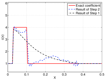
(a)

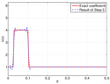
(b)

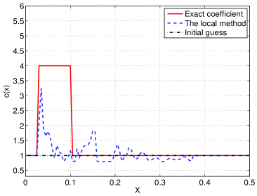
(c)

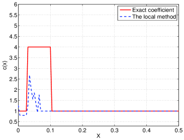
(d)

Figure 1: Reconstruction of the coefficient of Example 1. (a) Result of Steps 1 and 2, (b) Result of Step 3, (c) Result of Step 2 starting from the homogeneous medium as the first guess, (d) Result of Step 3 applied to the result of (c).

Since our target application is in imaging of an abnormal object placed in a homogeneous medium, we mainly test the proposed algorithm with a discontinuous coefficient. The locations of the discontinuities represent the location of the target. As mentioned in Remarks 6.1, it is hard to obtain accurate reconstructions at locations far away from the measurement point. However, this is not a serious restriction from the practical standpoint. Indeed, our experience of working with 3-d time resolved backscattering experimental data [5, 9, 10] tells us that, using the so-called data propagation procedure in data pre-processing, we can approximate quite well both the distance from the measurement point to the target and the Dirichlet and Neumann backscattering data near the target. Thus, we assume below that the target is close to the measurement point.

In the following examples, the parameters were chosen as follows: The pseudo frequencies were $s\in\left[4,15\right]$ with the integration step size in (13) $\Delta s=0.05$. The number of Laguerre’s functions was $N=11$. The coefficients $\lambda$ in the CWF was $\lambda=3$. The regularization parameter $\alpha=0.001$ and the truncation value $\epsilon=0.2$.

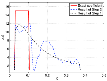
(a)

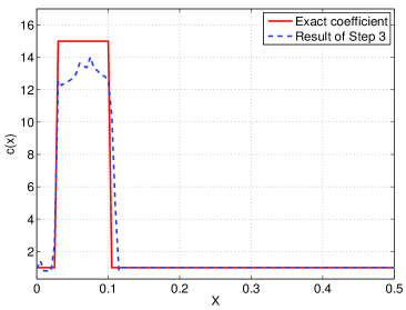
(b)

Figure 2: Reconstruction of the coefficient of Example 2. (a) Result of Steps 1 and 2, (b) Result of Step 3.

Example 1. Consider a piecewise constant coefficient given by $c(x)=1+3\chi[0.03,0.1],$ where $\chi$ is the characteristic function. Figure 1 (a) compares the computed coefficient values of Steps 1 and 2 with the exact one and Figure 1 (b) depicts the result of Step 3. To compare with the performance of the above locally convergent method alone, we plot in Figure 1 (c), (d) the results of Steps 2 and 3, respectively, starting from the homogeneous medium as the initial guess. We can see that our hybrid algorithm provided accurate results, whereas the locally convergent method alone failed.

Example 2. In this example, we consider another piecewise constant coefficient with a larger jump $c(x)=1+14\chi[0.03,0.1].$ The results of Steps 1 - 3 are shown in Figure 2. Even though the jump of the coefficient is high in this case, we still can see the good accuracy of the reconstruction using our hybrid algorithm.

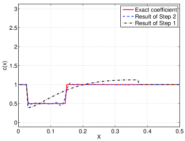
(a)

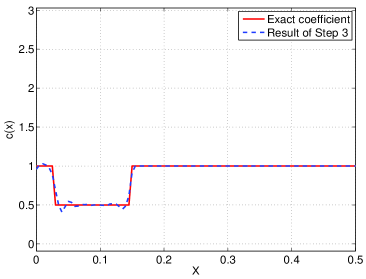
(b)

Figure 3: Reconstruction of the coefficient of Example 3. (a) Result of Steps 1 and 2, (b) Result of Step 3.

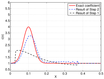
(a)

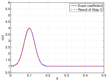
(b)

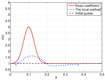
(c)

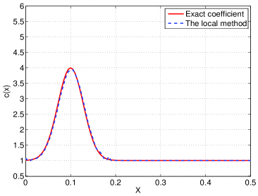
(d)

Figure 4: Reconstruction of the coefficient of Example 4. (a) Result of Steps 1 and 2, (b) Result of Step 3, (c) Result of Step 2 starting from the homogeneous medium as the first guess, (d) Result of Step 3 applied to the result of (c).

Example 3. Consider the exact coefficient $c(x)=1-0.5\chi[0.03,0.15].$ This coefficient mimics the case the case when the dielectric constant of an explosive is less than the one of a homogeneous background. Figure 3 shows the reconstruction results of Steps 1 - 3 of the algorithm. Again, we obtained an accurate reconstruction.

Example 4. Finally, we consider a continuous coefficient given by $c(x)=1+3e^{-(x-0.1)^{2}/\left(0.04\right)^{2}}.$ The results are shown in Figure 4. Comparing Figure 4 (a) with Figure 4 (c), one can see that the combination of Step 1 and Step 2 provided much better result than Step 2 starting from the homogeneous medium as the first guess. However, results of Step 3 of both cases are accurate.

From Figure 1 (d) and Figure 4 (d) we see that the above locally convergent method, taking alone, is unstable in the sense that, depending on the type of the target, it provides either bad or good quality images. Meanwhile, the proposed hybrid algorithm provides accurate results in all four examples.

References

- [1] M. Abramowitz and I. A. Stegun. Handbook of Mathematical Functions with Formulas, Graphs, and Mathematical Tables, volume 55 of National Bureau of Standards Applied Mathematics Series. 1964.
- [2] A. Bakushinsky, M. Y. Kokurin and A. Smirnova, Iterative Methods for Ill-Posed Problems, De Gruyter, 2011.
- [3] L. Beilina and M.V. Klibanov, Approximate Global Convergence and Adaptivity for Coefficient Inverse Problems, Springer, 2012.
- [4] L. Beilina, Energy estimates and numerical verification of the stabilized domain decomposition finite element/finite difference approach for the Maxwell’s system in time domain, Central European Journal of Mathematics, 11, 702-733, 2013.
- [5] L. Beilina, N.T. Thành, M.V. Klibanov and M.A. Fiddy, Reconstruction from blind experimental data for an inverse problem for a hyperbolic equation, Inverse Problems, 30, 025002, 2014.
- [6] B. Engquist and A. Majda, Absorbing boundary conditions for numerical simulation of waves, Proc. Natl. Acad. Sci. USA, 74, 1765–1766, 1977.
- [7] A.V. Kuzhuget, L. Beilina, M.V. Klibanov, A. Sullivan, L. Nguyen and M.A. Fiddy, Blind experimental data collected in the field and an approximately globally convergent inverse algorithm, Inverse Problems, 28, 095007, 2012.
- [8] M.V. Klibanov and A. Timonov, Carleman Estimates for Coefficient Inverse Problems and Numerical Applications, VSP, Utrecht, 2004.
- [9] N. T. Thành, L. Beilina, M. V. Klibanov and M. A. Fiddy, Reconstruction of the refractive index from experimental backscattering data using a globally convergent inverse method, SIAM J. Sci. Comp., 36, B273-B293, 2014.
- [10] N. T. Thành, L. Beilina, M. V. Klibanov and M. A. Fiddy, Imaging of buried objects from experimental backscattering time dependent measurements using a gloobally convergent inverse algorithm, arxiv: 1406.3500v1 [math-ph], 2014.