A Cyclic Coordinate Descent Algorithm for $l_{q}$ Regularization

Abstract

In recent studies on sparse modeling, $l_{q}$ ($0<q<1$) regularization has received considerable attention due to its superiorities on sparsity-inducing and bias reduction over the $l_{1}$ regularization. In this paper, we propose a cyclic coordinate descent (CCD) algorithm for $l_{q}$ regularization. Our main result states that the CCD algorithm converges globally to a stationary point as long as the stepsize is less than a positive constant. Furthermore, we demonstrate that the CCD algorithm converges to a local minimizer under certain additional conditions. Our numerical experiments demonstrate the efficiency of the CCD algorithm.

I Introduction

Recently, the sparse vector recovery problems have attracted lots of attention in both scientific research and engineering practice ([1]-[9]). Typical applications include compressed sensing [1], [2], statistical regression [5], visual coding [6], signal processing [7], machine learning [8], magnetic resonance imaging (MRI) [3] and microwave imaging [9], [10]. In a general setup, an unknown sparse vector $x\in\mathbf{R}^{N}$ is reconstructed from measurements

$$y=Ax,$$ (1)

or more generally, from

$$y=Ax+\epsilon,$$ (2)

where $y\in\mathbf{R}^{m}$, $A\in\mathbf{R}^{m\times N}$ (commonly, $m<N$) is a measurement matrix and $\epsilon$ represents the noise. The problem can be modeled as the $l_{0}$ regularization problem

$$\min_{x\in\mathbf{R}^{N}}\left\{\frac{1}{2}{\|Ax-y\|}_{2}^{2}+\lambda{\|x\|}_{0}\right\},$$ (3)

where $\|x\|_{0}$, formally called the $l_{0}$ norm, denotes the number of nonzero components of $x$, and $\lambda>0$ is a regularization parameter. However, due to its NP-hardness [11], $l_{0}$ regularization is generally intractable.

In order to overcome such difficulty, many continuous penalties were proposed to substitute the $l_{0}$ norm by the following optimization problem

$$\min_{x\in\mathbf{R}^{N}}\left\{\frac{1}{2}{\|Ax-y\|}_{2}^{2}+\lambda\Phi(x)\right\},$$ (4)

where $\Phi(x)$ is a separable, continuous penalty with $\Phi(x)=\sum_{i=1}^{N}\phi(x_{i})$, and $x=(x_{1},\cdots,x_{N})^{T}$. One of the most important cases is the $l_{1}$ norm, i.e., $\Phi(x)=\|x\|_{1}=\sum_{i=1}^{N}|x_{i}|$. The $l_{1}$ norm is convex and thus, the corresponding $l_{1}$ norm regularized convex optimization problem can be efficiently solved. Because of this, the $l_{1}$ norm gets its popularity and has been accepted as a very useful method for the modeling of the sparsity problems. Nevertheless, the $l_{1}$ norm may not induce further sparsity when applied to certain applications [12], [13], [14]. Alternatively, many non-convex penalties were introduced as relaxations of the $l_{0}$ norm. Among these, the $l_{q}$ norm with $0<q<1$ (not an actual norm when $0<q<1$), i.e., $\|x\|_{q}=(\sum_{i=1}^{N}|x_{i}|^{q})^{1/q}$ is one of the most typical subsitutions. Compared with the $l_{1}$ norm, the $l_{q}$ norm can usually induce better sparsity and reduce the bias while the corresponding non-convex regularized optimization problems are generally more difficult to solve.

Several classes of algorithms have been developed to solve the non-convex regularized optimization problem (4). These algorithms include half-quadratic (HQ) algorithm [15], [16], iteratively reweighted algorithm [12], [17], difference of convex functions algorithm (DC programming) [18], iterative thresholding algorithm [19], [20], [21], and cyclic coordinate descent (CCD) algorithm [22], [23].

The first class is the half-quadratic (HQ) algorithm [15], [16]. The basic idea of HQ algorithm is to formulate the original objective function as an infimum of a family of augmented functions via introducing a dual variable, and then minimize the augmented function along the primal and dual variables in an alternate fashion. However, HQ algorithms can be efficient only when both subproblems are easily solved (particularly, when both subproblems have the closed-form solutions). The second class is the iteratively reweighted algorithm which includes the iteratively reweighted least squares minimization (IRLS) [17], [24], [25], and iteratively reweighted $l_{1}$-minimization (IRL1) [12]. More specifically, the IRLS algorithm solves a sequence of weighted least squares problems, which can be viewed as some approximate problems to the original optimization problem. Similarly, the IRL1 algorithm solves a sequence of non-smooth weighted $l_{1}$-minimization problems, and hence can be seen as the non-smooth counterpart to the IRLS algorithm. Nevertheless, the iteratively reweighted algorithms can be only efficient when applied to such non-convex regularization problems whose non-convex penalty can be well approximated by the quadratic function or the weighted $l_{1}$ norm function.

The third class is the difference of convex functions algorithm (DC programming) [18], which is also called Multi-Stage (MS) convex relaxation [26]. The key idea of DC programming is to consider a proper decomposition of the objective function. More specifically, it converts the non-convex penalized problem into a convex reweighted $l_{1}$ minimization problem (called primal problem) and another convex problem (called dual problem), and then iteratively optimizes the primal and dual problems [18]. Hence, it can only be applied to a certain family of non-convex penalties that can be decomposed as a difference of convex functions. The fourth class is the iterative thresholding algorithm [20], [21], [27], [28], which fits the framework of the forward-backward splitting algorithm [29] and the framework of the generalized gradient projection algorithm [19]. Intuitively, the iterative thresholding algorithm can be seen as a procedure of Landweber iteration projected by a certain thresholding operator. Compared with the other types of non-convex algorithms, the iterative thresholding algorithm can be easily implemented and has relatively lower computational complexity for large scale problems [9], [10], [30]. However, the iterative thresholding algorithm can only be effectively applied to models with some particular structures.

The last class is the cyclic coordinate descent (CCD) algorithm. Basically, CCD algorithm is a coordinate descent algorithm with the cyclic coordinate updating rule. In [31], a CCD algorithm was implemented for solving the $l_{1}$ regularization problem. Its convergence can be shown by referring to [22]. In [32], a CCD algorithm was proposed for a class of non-convex penalized least squares problems. However, both [32] and [22] do not consider the CCD algorithm for $l_{q}$ regularization problem. Recently, Marjanovic and Solo [23] proposed a cyclic descent algorithm (called $l_{q}$CD) for the normalized $l_{q}$ regularization problem where the columns of $A$ are normalized with the unit $l_{2}$ norm, i.e., $\|A_{i}\|_{2}=1$, $i=1,2,\dots,N$, where $A_{i}$ is the $i$-th column of $A$. They proved the subsequential convergence and furthered the convergence to a local minimizer under the scalable restricted isometry property (SRIP) in [23]. According to [23], the column-normalization requirement is crucial for the convergence analysis of $l_{q}$CD algorithm. However, such requirement may limit the applicability of the $l_{q}$CD algorithm, and also will introduce some additional computational complexity.

In this paper, we propose a cyclic coordinate descent (CCD) algorithm (called CCD algorithm) for solving $l_{q}$ regularization problem without the requirement of column-normalization. Instead, we introduce a stepsize parameter to improve the applicability of the CCD algorithm. The proposed CCD algorithm can be viewed as a variant of the $l_{q}$CD algorithm. In the perspective of algorithmic implementation, it can be noted that the $l_{q}$CD algorithm proposed in [23] is actually a special case of the proposed CCD algorithm with the stepsize as 1 and a column-normalized $A$. More important, we can justify the convergence instead of the subsequential convergence of the proposed CCD algorithm via introducing a stepsize parameter. We prove that the proposed CCD algorithm can converge to a stationary point as long as the stepsize less than $\frac{1}{L_{\max}}$ with $L_{\max}=\max_{i}\|A_{i}\|_{2}^{2}$. This convergence condition is generally weaker than those of the iterative thresholding algorithms, i.e., the stepsize parameter should be less than $\|A\|_{2}^{-2}$ [21], [34]. Roughly, the proposed CCD algorithm is a Gauss-Seidel iterative method while the corresponding iterative thresholding algorithm is a Jacobi iterative algorithm. We can also justify that the proposed CCD algorithm converges to a local minimizer under some additional conditions. In addition, it can be observed numerically that the proposed CCD algorithm has almost the same performance of the $l_{q}$CD algorithm when $A$ is normalized in column and the stepsize approaches to 1.

The reminder of this paper is organized as follows. In section II, we first introduce the $l_{q}$ $(0<q<1)$ regularization problem, then propose a cyclic coordinate descent algorithm for such a non-convex regularization problem. In section III, we prove the convergence of the proposed CCD algorithm. In section IV, we implement a series of simulations to demonstrate the efficiency of the CCD algorithm. We conclude this paper in section V.

Notations: We denote $\mathbf{N}$ and $\mathbf{R}$ as the natural number set and one-dimensional real space, respectively. Given an index set $I\subset\{1,2,\cdots,N\}$, $I^{c}$ represents its complementary set, i.e., $I^{c}=\{1,2,\cdots,N\}\setminus I.$ For any matrix $A\in\mathbf{R}^{M\times N}$, $A_{i}$ denotes as the $i$-th column of $A$, and $A_{I}$ represents a submatrix of $A$ with the columns restricted to an index set $I$. Similarly, for any vector $x\in\mathbf{R}^{N}$, $x_{i}$ denotes as the $i$-th component of $x$, and $x_{I}$ represents a subvector of $x$ with the coordinate coefficients restricted to $I$. For any matrix and vector, we denote $\cdot^{T}$ by the transpose operation. For any square matrix $A$, $\sigma_{i}(A)$ and $\sigma_{\min}(A)$ denote as the $i$-th and the minimal eigenvalues of $A$, respectively.

II A Cyclic Coordinate Descent Algorithm

In this section, we first introduce the non-convex $l_{q}$ regularization ($0<q<1$) problem, then show some important theoretical results of the $l_{q}$ regularization problem, which serve as the basis of the following sections. Finally, we propose a cyclic coordinate descent (CCD) algorithm for solving the $l_{q}$ regularization problem.

II-A $l_{q}$ Regularization Problem

Mathematically, the $l_{q}$ regularization problem is

$$\min_{x\in\mathbf{R}^{N}}\left\{T_{\lambda}(x)=\frac{1}{2}{\|Ax-y\|}_{2}^{2}+\lambda\|x\|_{q}^{q}\right\},$$ (5)

where $0<q<1$ and $\lambda>0$. It can be easily observed that the first least squares term is proper lower semi-continuous while the $l_{q}$ penalty is continuous and coercive, and thus the minimum of the $l_{q}$ regularization problem exists. However, due to the non-convexity, the $l_{q}$ regularization problem might have several global minimizers.

For better characterizing the global minimizers of (5), we first generalize the proximity operator from convex case to the non-convex $l_{q}$ norm,

$$Prox_{\lambda\mu,q}(x)=\arg\min_{u\in\mathbf{R}^{N}}\left\{\frac{\|x-u\|_{2}^{2}}{2}+\lambda\mu\|u\|_{q}^{q}\right\},$$ (6)

where $\mu>0$ is the stepsize parameter. Since $\|\cdot\|_{q}^{q}$ is separable, thus computing $Prox_{\lambda\mu,q}$ is reduced to solve a one-dimensional minimization problem, that is,

$$prox_{\lambda\mu,q}(z)=\arg\min_{v\in\mathbf{R}}\left\{\frac{|z-v|^{2}}{2}+\lambda\mu|v|^{q}\right\},$$ (7)

and thus,

$$Prox_{\lambda\mu,q}(x)=(prox_{\lambda\mu,q}(x_{1}),\cdots,prox_{\lambda\mu,q}(x_{N}))^{T}.$$ (8)

Furthermore, according to [19], $prox_{\lambda\mu,q}(\cdot)$ can be expressed as follows:
$prox_{\lambda\mu,q}(z)=$

$$\left\{\begin{array}[c]{ll}(\cdot+\lambda\mu qsgn(\cdot)|\cdot|^{q-1})^{-1}(z),&\mbox{for}\ |z|\geq\tau_{\mu,q}\\ 0,&\mbox{for}\ |z|\leq\tau_{\mu,q}\end{array}\right.$$ (9)

for any $z\in\mathbf{R}$ with

$$\tau_{\mu,q}=\frac{2-q}{2-2q}(2\lambda\mu(1-q))^{\frac{1}{2-q}},$$ (10)

$$\eta_{\mu,q}=(2\lambda\mu(1-q))^{\frac{1}{2-q}},$$ (11)

and the range domain of $prox_{\lambda\mu,q}$ is $\{0\}\cup[\eta_{\mu,q},\infty)$, $sgn(\cdot)$ represents the sign function henceforth. When $\ |z|\geq\tau_{\mu,q}$, the relation $prox_{\lambda\mu,q}(z)=(\cdot+\lambda\mu qsgn(\cdot)|\cdot|^{q-1})^{-1}(z)$ means that $prox_{\lambda\mu,q}(z)$ satisfies the following equation

$$v+\lambda\mu q\cdot sgn(v)|v|^{q-1}=z.$$

Remark 1.

From (9), it can be noted that $prox_{\lambda\mu,q}$ is a set-valued operator since it can take two different function values when $|z|=\tau_{\mu,q}.$ Moreover, for some specific $q$ (say, $q=1/2,2/3$), the operator $prox_{\lambda\mu,q}(\cdot)$ can be expressed analytically, which are shown as follows:

(a) $prox_{\lambda\mu,1/2}(\cdot)$ for $l_{1/2}$ regularization ([20]):
$prox_{\lambda\mu,1/2}(z)=$

$$\\ \left\{\begin{array}[]{cc}{\frac{2}{3}}z\left(1+\cos\left({\frac{2{\pi}}{3}}-{\frac{2}{3}}\theta_{\tau_{\mu,1/2}}(z)\right)\right),&|z|\geq\tau_{\mu,1/2}\\ 0,&|z|\leq\tau_{\mu,1/2}\end{array}\right.,$$ (12)

with $\theta_{\tau_{\mu,1/2}}(z)=\arccos\left({\frac{\sqrt{2}}{2}}{(\frac{\tau_{\mu,1/2}}{|z|})}^{\frac{3}{2}}\right).$

(b) $prox_{\lambda\mu,2/3}(\cdot)$ for $l_{2/3}$ regularization ([35]):
$prox_{\lambda\mu,2/3}(z)=$

$$\left\{\begin{array}[]{cc}sgn(z)\left(\frac{\phi_{\tau_{\mu,2/3}}(z)+\sqrt{f_{\tau_{\mu,2/3}}(z)}}{2}\right)^{3},&|z|\geq\tau_{\mu,2/3}\\ 0,&|z|\leq\tau_{\mu,2/3}\end{array}\right.,$$ (13)

where

$$f_{\tau_{\mu,2/3}}(z)=\frac{2|z|}{\phi_{\tau_{\mu,2/3}}(z)}-\phi_{\tau_{\mu,2/3}}(z)^{2},$$

and

$$\phi_{\tau_{\mu,2/3}}(z)=\frac{2^{13/16}}{4\sqrt{3}}\tau_{\mu,2/3}^{3/16}(\cosh(\frac{\theta_{\tau_{\mu,2/3}}(z)}{3}))^{1/2}$$

with $\theta_{\tau_{\mu,2/3}}(z)=arccosh(\frac{3\sqrt{3}z^{2}}{2^{7/4}(2\tau_{\mu,2/3})^{9/8}})$.

Remark 2.

It was demonstrated in [20] that $prox_{\lambda\mu,q}(\cdot)$ has analytical expression when $q$ is $\frac{1}{2}$ or $\frac{2}{3}$. While for other $q\in(0,1)$, we can use an iterative scheme proposed by [23] to compute the operator $prox_{\lambda\mu,q}(\cdot)$, that is, let $\eta_{\mu,q}\leq v^{0}\leq|z|$,

$$v^{k+1}=|z|-\lambda\mu q|v^{k}|^{q-1}.$$

With the definition of proximity operator, we can define a new operator $G_{\lambda\mu,q}(\cdot)$ as

$$G_{\lambda\mu,q}(x)=Prox_{\lambda\mu,q}(x-\mu A^{T}(Ax-y))$$ (14)

for any $x\in\mathbf{R}^{N}$. We denote ${\mathcal{F}}_{q}$ as the fixed point set of the operator $G_{\lambda\mu,q}$, i.e.,

$${\mathcal{F}}_{q}=\{x:x=G_{\lambda\mu,q}(x)\}.$$ (15)

According to [19], each global minimizer of (5) is a fixed point of $G_{\lambda\mu,q}(\cdot)$, which is shown as follows.

Lemma 1.

(Proposition 2.3 in [19]). Assume that $0<\mu<\|A\|_{2}^{-2}$, then each global minimizer of $T_{\lambda}$ is a fixed point of $G_{\lambda\mu,q}(\cdot)$.

By the definition of $Prox_{\lambda\mu,q}$, a type of optimality conditions of $l_{q}$ regularization has been derived in [23].

Lemma 2.

(Theorem 3 in [23]). Given a point $x^{*}$, define the support set of $x^{*}$ as $Supp(x^{*})=\{i:x_{i}^{*}\neq 0\}$, then $x^{*}\in{\mathcal{F}}_{q}$ if and only if the following three conditions hold.

1. For $i\in Supp(x^{*})$, $|x_{i}^{*}|\geq\eta_{\mu,q}$.

2. For $i\in Supp(x^{*})$, $A_{i}^{T}(Ax^{*}-y)+\lambda qsgn(x_{i}^{*})|x_{i}^{*}|^{q-1}=0$.

3. For $i\in Supp(x^{*})^{c}$, $|A_{i}^{T}(Ax^{*}-y)|\leq\tau_{\mu,q}/\mu$.

We call the point a stationary point of the $l_{q}$ regularization problem henceforth if it satisfies the optimality conditions in Lemma 2.

II-B A CCD Algorithm for $l_{q}$ Regularization

In this subsection, we derive a cyclic coordinate descent algorithm for solving the $l_{q}$ regularization problem. More specifically, given the current iterate $x^{n}$, at the next iteration, the $i$-th coefficient is selected by

$$i=\left\{\begin{array}[]{cc}N&{\rm if}\ 0\equiv{(n+1)}\ {\rm mod}\ N\\ {(n+1)}\ {\rm mod}\ N,&{\rm otherwise}\end{array}\right.$$ (16)

and then updated by

$$x_{i}^{n+1}\in\arg\min_{v\in\mathbf{R}}\left\{\frac{|z^{n}_{i}-v|^{2}}{2}+\lambda\mu|v|^{q}\right\}=prox_{\lambda\mu,q}(z^{n}_{i}),$$

where

$$z_{i}^{n}=x_{i}^{n}-\mu A_{i}^{T}(Ax^{n}-y).$$ (17)

It can be seen from (9) that $prox_{\lambda\mu,q}$ is a set-valued operator. Therefore, we select a particular single-valued operator of $prox_{\lambda\mu,q}$ and then update $x_{i}^{n+1}$ according to the following scheme,

$$x^{n+1}_{i}=\mathcal{T}(z_{i}^{n},x_{i}^{n}),$$ (18)

where

$$\mathcal{T}(z_{i}^{n},x_{i}^{n})=\left\{\begin{array}[]{cc}prox_{\lambda\mu,q}(z_{i}^{n})&{\rm if}\ |z_{i}^{n}|\neq\tau_{\mu,q}\\ sgn(z_{i}^{n})\eta_{\mu,q}\mathbf{I}(x_{i}^{n}\neq 0),&{\rm if}\ |z_{i}^{n}|=\tau_{\mu,q}\end{array}\right.,$$

and $\mathbf{I}(x_{i}^{n}\neq 0)$ denotes the indicator function, that is,

$$\mathbf{I}(x_{i}^{n}\neq 0)=\left\{\begin{array}[]{cc}1,&{\rm if}\ x_{i}^{n}\neq 0\\ 0,&{\rm otherwise}\end{array}\right..$$

While the other components of $x^{n+1}$ are being fixed, i.e.,

$$x_{j}^{n+1}=x_{j}^{n},\ {\rm for}\ j\neq i.$$ (19)

In summary, we can formulate the proposed algorithm as follows.

The Cyclic Coordinate Descent (CCD) Algorithm

Initialize with $x^{0}$. Choose a stepsize $\mu>0$, let $n:=0$.

Step 1. Calculate the index $i$ according to (16);

Step 2. Calculate $z_{i}^{n}$ according to (17);

Step 3. Update $x_{i}^{n+1}$ via (18) and $x_{j}^{n+1}=x_{j}^{n}$ for $j\neq i$;

Step 4. Check the terminational rule. If yes, stop;

otherwise, let $n:=n+1$, go to Step 1.

Remark 3.

It can be observed that the proposed algorithm is similar to the $l_{q}$CD proposed by Marjanovic and Solo [23]. However, we get rid of the column-normalization requirement of $A$ by introducing a stepsize parameter $\mu$. The following sections show that it can bring more benefits in both algorithmic implementation and theoretical justification.

III Convergence Analysis

In this section, we prove the convergence of the proposed CCD algorithm for the $l_{q}$ regularization problem with $0<q<1$. We first give some basic properties of the proposed algorithm, which serve as the basis of the next subsections, and then prove that the CCD algorithm converges to a stationary point from any initial point as long as the stepsize parameter $\mu$ is less than a positive constant, and finally show that the proposed algorithm converges to a local minimizer under certain additional conditions.

III-A Some Basic Properties of CCD Algorithm

According to the definition of the operator $prox_{\lambda\mu,q}(\cdot)$ (9) and the updating rule of CCD algorithm (16)-(19), we can claim that $x_{i}^{n+1}$ satisfies the following property.

Property 1.

Given the current iterate $x^{n}$ ($n\in\mathbf{N}$), the index set $i$ is determined via (16), then $x_{i}^{n+1}$ satisfies either

1. $x_{i}^{n+1}=0,$ or,

2. $|x_{i}^{n+1}|\geq\eta_{\mu,q}$ and also satisfies the following equation

   $$A_{i}^{T}(Ax^{n+1}-y)+\lambda qsgn(x_{i}^{n+1})|x_{i}^{n+1}|^{q-1}$$

   $$=(\frac{1}{\mu}-A_{i}^{T}A_{i})(x_{i}^{n}-x_{i}^{n+1}).$$ (20)

   that is, $\nabla_{i}T_{\lambda}(x^{n+1})=(\frac{1}{\mu}-A_{i}^{T}A_{i})(x_{i}^{n}-x_{i}^{n+1}),$ where $\nabla_{i}T_{\lambda}(x^{n+1})$ represents the gradient of $T_{\lambda}$ with respect to the $i$-th coordinate at the point $x^{n+1}$.

Proof.

According to (9) and (18), it holds obviously either $x_{i}^{n+1}=0$ or $|x_{i}^{n+1}|\geq\eta_{\mu,q}$. Moreover, when $|x_{i}^{n+1}|\geq\eta_{\mu,q}$, according to (7), $x_{i}^{n+1}$ is a minimizer of the optimization problem (7) with $z=z_{i}^{n}$. Therefore, $x_{i}^{n+1}$ should satisfy the following optimality condition

$$x_{i}^{n+1}-z_{i}^{n}+\lambda\mu qsgn(x_{i}^{n+1})|x_{i}^{n+1}|^{q-1}=0.$$ (21)

Plugging (17) into (21) gives

$$A_{i}^{T}(Ax^{n+1}-y)+\lambda qsgn(x_{i}^{n+1})|x_{i}^{n+1}|^{q-1}$$

$$=\frac{1}{\mu}(x_{i}^{n}-x_{i}^{n+1})-A_{i}^{T}A(x^{n}-x^{n+1}).$$ (22)

Combining (19) and (22) implies (20). ∎

As shown by Property 1, the coordinate-wise gradient of $T_{\lambda}$ with respect to the $i$-th coordinate at $x^{n+1}$ is not exact zero but with a relative error. In the following, we show that the sequence $\{T_{\lambda}(x^{n})\}$ satisfies the sufficient decrease property [33].

Property 2.

Let $\{x^{n}\}$ be a sequence generated by the CCD algorithm. Assume that $0<\mu<L_{\max}^{-1}$, then

$$T_{\lambda}(x^{n})-T_{\lambda}(x^{n+1})\geq\frac{1}{2}(\frac{1}{\mu}-L_{\max})\|x^{n}-x^{n+1}\|_{2}^{2},~{}\forall n\in\mathbf{N}.$$

Proof.

Given the current iteration $x^{n}$, let the coefficient index $i$ be determined according to (16). According to (7) and (18),

$$x_{i}^{n+1}\in\arg\min_{v\in\mathbf{R}}\left\{\frac{|z_{i}^{n}-v|^{2}}{2}+\lambda\mu|v|^{q}\right\},$$

where $z_{i}^{n}=x_{i}^{n}-\mu A_{i}^{T}(Ax^{n}-y)$. Then it implies

$$\frac{1}{2}|\mu A_{i}^{T}(Ax^{n}-y)|^{2}+\lambda\mu|x_{i}^{n}|^{q}$$

$$\geq\frac{1}{2}|(x_{i}^{n+1}-x_{i}^{n})+\mu A_{i}^{T}(Ax^{n}-y)|^{2}+\lambda\mu|x_{i}^{n+1}|^{q}.$$

Some simplifications give

$$\lambda|x_{i}^{n}|^{q}-\lambda|x_{i}^{n+1}|^{q}$$

$$\geq\frac{|x_{i}^{n+1}-x_{i}^{n}|^{2}}{2\mu}+A_{i}^{T}(Ax^{n}-y)(x_{i}^{n+1}-x_{i}^{n}).$$ (23)

Moreover, since $x_{j}^{n+1}=x_{j}^{n}$ for any $j\neq i$, (23) becomes

$$\lambda\|x^{n}\|_{q}^{q}-\lambda\|x^{n+1}\|_{q}^{q}$$

$$\geq\frac{\|x^{n+1}-x^{n}\|^{2}}{2\mu}+\langle Ax^{n}-y,A(x^{n+1}-x^{n})\rangle.$$ (24)

Adding $\frac{1}{2}\|Ax^{n}-y\|_{2}^{2}-\frac{1}{2}\|Ax^{n+1}-y\|_{2}^{2}$ to both sides of (24) gives

$$T_{\lambda}(x^{n})-T_{\lambda}(x^{n+1})$$

$$\geq\frac{\|x^{n+1}-x^{n}\|^{2}}{2\mu}-\frac{1}{2}\|A(x^{n}-x^{n+1})\|_{2}^{2}$$

$$=\frac{\|x^{n+1}-x^{n}\|^{2}}{2\mu}-\frac{1}{2}(A_{i}^{T}A_{i})\|x^{n}-x^{n+1}\|_{2}^{2}$$

$$\geq\frac{1}{2}(\frac{1}{\mu}-L_{\max})\|x^{n}-x^{n+1}\|_{2}^{2},$$ (25)

where the first equality holds for

$$\|A(x^{n}-x^{n+1})\|_{2}^{2}=(A_{i}^{T}A_{i})|x_{i}^{n}-x_{i}^{n+1}|^{2}=(A_{i}^{T}A_{i})\|x^{n}-x^{n+1}\|_{2}^{2},$$

and the second inequality holds for $A_{i}^{T}A_{i}\leq L_{\max}$. ∎

In fact, by the first inequality of (25), a slightly stricter but more commonly used condition to guarantee the sufficient decrease is $0<\mu<\|A\|_{2}^{-2}.$ Property 2, gives the boundedness of the sequence $\{x^{n}\}$.

Property 3.

Let $\{x^{n}\}$ be a sequence generated by the CCD algorithm. Assume that $0<\mu<L_{\max}^{-1}$ and $T_{\lambda}(x^{0})<+\infty$, then $x^{n}$ is bounded for any $n\in\mathbf{N}$.

Proof.

By Property 2, for any $n$,

$$\|x^{n}\|_{q}^{q}\leq\frac{1}{\lambda}T_{\lambda}(x^{n})\leq\frac{1}{\lambda}T_{\lambda}(x^{0})<+\infty.$$

It implies that $x^{n}$ is bounded. ∎

Moreover, Property 2 also gives the following asymptotically regular property.

Property 4.

Let $\{x^{n}\}$ be a sequence generated by the CCD algorithm. Assume $0<\mu<L_{\max}^{-1}$, then

$$\sum_{k=0}^{n}\|x^{k+1}-x^{k}\|_{2}^{2}\leq\frac{2\mu}{1-\mu L_{\max}}T_{\lambda}(x^{0}),$$

and

$$\|x^{n}-x^{n+1}\|_{2}\rightarrow 0,\ {\rm as}\ n\rightarrow+\infty.$$

From Properties 2-4, we can prove the subsequential convergence of the CCD algorithm.

Theorem 1.

Let $\{x^{n}\}$ be a sequence generated by the CCD algorithm. Assume that $0<\mu<L_{\max}^{-1}$ and $T_{\lambda}(x^{0})<+\infty$, then the sequence $\{x^{n}\}$ has a convergent subsequence. Moreover, let $\mathcal{L}$ be the set of the limit points of $\{x^{n}\}$, then $\mathcal{L}$ is closed and connected.

Proof.

By Property 2, we know that $\{T_{\lambda}(x^{n})\}$ is a decreasing and lower-bounded sequence, thus, $\{T_{\lambda}(x^{n})\}$ is convergent. Denote the convergent value of $\{T_{\lambda}(x^{n})\}$ as $T^{*}$. Moreover, by Property 3, $\{x^{n}\}$ is bounded, and also by the continuity of $T_{\lambda}(\cdot)$, there exists a subsequence of $\{x^{n}\}$, $\{x^{n_{j}}\}$ converging to some point $x^{*}$, which satisfies $T_{\lambda}(x^{*})=T^{*}$.

Furthermore, by Property 4 and Ostrowski’s result (Theorem 26.1, p. 173) [36], the limit point set $\mathcal{L}$ of the sequence $\{x^{n}\}$ is closed and connected. ∎

Theorem 1 only shows the subsequential convergence of the CCD algorithm. Moreover, we note that $\mathcal{L}$ might not be a set of isolated points. Due to this, it becomes challenging to justify the global convergence of CCD algorithm. More specifically, there are still two open questions on the convergence of the CCD algorithm.

1. When does the algorithm converge globally? So far, for most non-convex algorithms, only subsequential convergence can be claimed.

2. Where does the algorithm converge? Does the algorithm converge to a global minimizer or more practically, a local minimizer due to the non-convexity of the optimization problem?

III-B Convergence To A Stationary Point

In this subsection, we will focus on answering the first open question proposed in the end of the last subsection. More specifically, we will show that the whole sequence $\{x^{n}\}$ generated by the CCD algorithm converges to a stationary point as long as the stepsize parameter $\mu$ satisfies $0<\mu<\frac{1}{L_{\max}}$.

Given the current iteration $x^{n}$, we define the descent function as

$$\Delta(x^{n},x^{n+1})=T_{\lambda}(x^{n})-T_{\lambda}(x^{n+1}).$$ (26)

Note that $x^{n}$ and $x^{n+1}$ differ only in their $i$-th coefficient which is determined by (16). From now on, if not stated, it is assumed $x_{i}^{n+1}$ is given by (18) and $i$ is given by (16). The following lemma gives an important property of the descent function.

Lemma 3.

Let $\{x^{n}\}$ be a sequence generated by CCD algorithm. Assume that $0<\mu<L_{\max}^{-1}$, then

$$\Delta(x^{n},x^{n+1})=0\ {\rm if~{}and~{}only~{}if}\ x_{i}^{n+1}=x_{i}^{n}.$$

Proof.

($\Rightarrow$) It is obvious that if $x_{i}^{n+1}=x_{i}^{n}$, then $x^{n+1}=x^{n}$, and thus $\Delta(x^{n},x^{n+1})=0$.

($\Leftarrow$) If $\Delta(x^{n},x^{n+1})=0$, then Property 2 implies $x^{n+1}=x^{n}$ and thus, $x_{i}^{n+1}=x_{i}^{n}$. ∎

Moreover, similar to Theorem 10 in [23], we can claim that the mapping $\mathcal{T}(\cdot,\cdot)$ is a closed mapping, shown as follows.

Lemma 4.

$\mathcal{T}(\cdot,\cdot)$ is a closed mapping, i.e., assume

1. $x_{i}^{n}\rightarrow x_{i}^{*}$ as $n\rightarrow\infty;$

2. $x_{i}^{n+1}\rightarrow x_{i}^{**}$ as $n\rightarrow\infty$, where $x_{i}^{n+1}=\mathcal{T}(z_{i}^{n},x_{i}^{n}).$

Then $x_{i}^{**}=\mathcal{T}(z_{i}^{*},x_{i}^{*})$, where $z_{i}^{*}=x_{i}^{*}-\mu A_{i}^{T}(Ax^{*}-y)$.

The proof is the essentially the same as that of Theorem 10 in [23]. The only difference is that $prox_{\lambda\mu,q}$ is discontinuous at $\tau_{\mu,q}$ while $prox_{\lambda,q}$ is discontinuous at $\tau_{1,q}$. Therefore, the closedness of the operator $\mathcal{T}(\cdot,\cdot)$ can not be changed after introducing a stepsize $\mu$. The following theorem shows that any limit point of the sequence $\{x^{n}\}$ is a stationary point of the non-convex $l_{q}$ regularization problem.

Theorem 2.

Let $\{x^{n}\}$ be a sequence generated by the CCD algorithm, and $\mathcal{L}$ be its limit point set. Assume that $0<\mu<L_{\max}^{-1}$ and $T_{\lambda}(x^{0})<+\infty$, then $\mathcal{L}\subseteq{\mathcal{F}}_{q}$.

The proof of this theorem is similar to that of Theorem 5 in [23]. For the completion, we provide the proof as follows.

Proof.

Since the sequence $\{x^{n}\}$ is bounded, then it has limit points. Let $x^{*}\in\mathcal{L}$. We now focus on the $i$-th coefficient of the sequence with $n=n(i)=jN+i-1$, where $i=1,2,\dots,N$ and $j=0,1,\dots.$ However, here, we simply use $n$ by which we mean $n(i)$. Now there exists a subsequence $\{x^{n_{1}},x^{n_{2}},\cdots\}$ such that

$$\{x^{n_{1}},x^{n_{2}},\cdots\}\rightarrow x^{*}\ {\rm and}\ \{x_{i}^{n_{1}},x_{i}^{n_{2}},\cdots\}\rightarrow x_{i}^{*}.$$ (27)

Moreover, since the sequence $\{x^{n_{1}+1},x^{n_{2}+1},\cdots\}$ is also bounded, thus, it also has limit points. Denoting one of these by $x^{**}$, then there exists a subsequence $\{x^{l_{1}+1},x^{l_{2}+1},\cdots\}$ such that

$$\{x^{l_{1}+1},x^{l_{2}+1},\cdots\}\rightarrow x^{**}\ {\rm and}\ \{x_{i}^{l_{1}+1},x_{i}^{l_{2}+1},\cdots\}\rightarrow x_{i}^{**},$$ (28)

where $\{l_{1},l_{2},\cdots\}\subset\{n_{1},n_{2},\cdots\}$. In this case, it holds

$$\{x^{l_{1}},x^{l_{2}},\cdots\}\rightarrow x^{*}\ {\rm and}\ \{x_{i}^{l_{1}},x_{i}^{l_{2}},\cdots\}\rightarrow x_{i}^{*},$$ (29)

since it is a subsequence of (27). From (17) and (29), we have

$$z_{i}^{l_{j}}\rightarrow z_{i}^{*}\ {\rm as}\ j\rightarrow\infty.$$

Thus, by Lemma 4, it holds

$$x_{i}^{**}=\mathcal{T}(z_{i}^{*},x_{i}^{*}).$$ (30)

Moreover, by (28), (29) and (19), it holds

$$x_{j}^{*}=x_{j}^{**}\ {\rm for}\ j\neq i.$$ (31)

In the following, by the continuity of $T_{\lambda}(\cdot)$ and thus the continuity of $\Delta(\cdot,\cdot)$ with respect to its arguments, it holds

$$\Delta(x^{l_{j}},x^{l_{j}+1})\rightarrow\Delta(x^{*},x^{**}).$$

Moreover, since the sequence $\{T_{\lambda}(x^{n})\}$ is convergent, then

$$\Delta(x^{l_{j}},x^{l_{j}+1})=T_{\lambda}(x^{l_{j}})-T_{\lambda}(x^{l_{j}+1})\rightarrow 0\ {\rm as}\ j\rightarrow\infty,$$

which implies

$$\Delta(x^{*},x^{**})=0.$$

Furthermore, by Lemma 3, and (30)-(31), it holds

$$x_{i}^{**}=x_{i}^{*}.$$ (32)

Combining (30) and (32), we have

$$x_{i}^{*}=\mathcal{T}(z_{i}^{*},x_{i}^{*}).$$ (33)

Since $i$ is arbitrary, we have that (33) holds for all $i\in\{1,\cdots,N\}$. It implies that $x^{*}$ is a fixed point of $G_{\lambda\mu,q}(\cdot)$, that is, $x^{*}\in{\mathcal{F}}_{q}$. Similarly, since $x^{*}\in\mathcal{L}$ is also arbitrary, therefore, $\mathcal{L}\subset{\mathcal{F}}_{q}$. Consequently, we complete the proof of this theorem. ∎

In the following theorem, we demonstrate the finite support convergence of the sequence $\{x^{n}\}$, that is, the support of $\{x^{n}\}$ will converge within a finite number of iterations. Denote $I^{n}=Supp(x^{n})=\{i:|x_{i}^{n}|\neq 0,i=1,2\cdots,N\}$, $I=Supp(x^{*})$.

Theorem 3.

Let $\{x^{n}\}$ be a sequence generated by the CCD algorithm. Assume that $0<\mu<\frac{1}{L_{\max}}$ and $x^{*}$ is a limit point of $\{x^{n}\}$, then there exists a sufficiently large positive integer $n^{*}>N$ such that when $n>n^{*}$, it holds

1. either $x_{j}^{n}=0$ or $|x_{j}^{n}|\geq\eta_{\mu,q}$ for $j=1,2,\cdots,N;$

2. $I^{n}=I$;

3. $sgn(x^{n})=sgn(x^{*})$.

Proof.

We can note that all the coefficient indices will be updated at least one time when $n>N$. By Property 1, once the index $i$ is updated at $n$-th iteration, then the coefficient $x_{i}^{n}$ satisfies:

$${\rm either}\ x_{i}^{n}=0\ {\rm or}\ |x_{i}^{n}|\geq\eta_{\mu,q}.$$

Thus, Theorem 3(a) holds.

In the following, we prove Theorem 3(b) and (c). By the assumption of Theorem 3, there exits a subsequence $\{x^{n_{j}}\}$ converges to $x^{*}$, i.e.,

$$x^{n_{j}}\rightarrow x^{*}\ \ \text{as}\ \ j\rightarrow\infty.$$ (34)

Thus, there exists a sufficiently large positive integer $j_{0}$ such that $\|x^{n_{j}}-x^{*}\|_{2}<\eta_{\mu,q}$ when $j\geq j_{0}$. Moreover, by Property 4, there also exists a sufficiently large positive integer $n^{*}>N$ such that $\|x^{n}-x^{n+1}\|_{2}<\eta_{\mu,q}$ when $n>n^{*}$. Without loss of generality, we let $n^{*}=n_{j_{0}}$. In the following, we first prove that $I^{n}=I$ and $sgn(x^{n})=sgn(x^{*})$ whenever $n>n^{*}$.

In order to prove $I^{n}=I$, we first show that $I^{n_{j}}=I$ when $j\geq j_{0}$ and then verify that $I^{n+1}=I^{n}$ when $n>n^{*}$. We now prove by contradiction that $I^{n_{j}}=I$ whenever $j\geq j_{0}$. Assume this is not the case, namely, that $I^{n_{j}}\neq I$. Then we easily derive a contradiction through distinguishing the following two possible cases:

Case 1: $I^{n_{j}}\neq I$ and $I^{n_{j}}\cap I\subset I^{n_{j}}.$ In this case, then there exists an $i_{n_{j}}$ such that $i_{n_{j}}\in I^{n_{j}}\setminus I$. By Theorem 3(a), it then implies

$$\|x^{n_{j}}-x^{\ast}\|_{2}\geq|x_{i_{n_{j}}}^{n_{j}}|\geq\min_{i\in I^{n_{j}}}|x_{i}^{n_{j}}|\geq\eta_{\mu,q},$$

which contradicts to $\|x^{n_{j}}-x^{\ast}\|_{2}<\eta_{\mu,q}.$

Case 2: $I^{n_{j}}\neq I$ and $I^{n_{j}}\cap I=I^{n_{j}}.$ In this case, it is obvious that $I^{n_{j}}\subset I$. Thus, there exists an $i^{\ast}$ such that $i^{\ast}\in I\setminus I^{n_{j}}$. By Lemma 2(a), we still have

$$\|x^{n_{j}}-x^{\ast}\|_{2}\geq|x_{i^{\ast}}^{\ast}|\geq\min_{i\in I}|x_{i}^{\ast}|\geq\eta_{\mu,q},$$

and it contradicts to $\|x^{n_{j}}-x^{\ast}\|_{2}<\eta_{\mu,q}$.

Thus we have justified that $I^{n_{j}}=I$ when $j\geq j_{0}$. Similarly, it can be also claimed that $I^{n+1}=I^{n}$ whenever $n>n^{*}$. Therefore, whenever $n>n^{*}$, it holds $I^{n}=I$.

As $I^{n}=I$ when $n>n^{*}$, it suffices to test that $sgn(x_{i}^{(n)})=sgn(x_{i}^{\ast})$ for any $i\in I$. Similar to the first part of proof, we will first check that $sgn(x_{i}^{n_{j}})=sgn(x_{i}^{*})$, and then $sgn(x_{i}^{n+1})=sgn(x_{i}^{n})$ for any $i\in I$ by contradiction. We now prove $sgn(x_{i}^{n_{j}})=sgn(x_{i}^{*})$ for any $i\in I$. Assume this is not the case. Then there exists an $i^{\ast}\in I$ such that $sgn(x_{i^{*}}^{n_{j}})\neq sgn(x_{i^{*}}^{\ast})$, and hence,

$$sgn(x_{i^{\ast}}^{n_{j}})sgn(x_{i^{\ast}}^{\ast})=-1.$$

From Lemma 2(a) and Theorem 3(a), it then implies

$$\|x^{n_{j}}-x^{\ast}\|_{2} \geq|x_{i^{\ast}}^{n_{j}}-x_{i^{\ast}}^{\ast}|=|x_{i^{\ast}}^{n_{j}}|+|x_{i^{\ast}}^{\ast}|$$

$$\geq\min_{i\in I}\{|x_{i}^{n_{j}}|+|x_{i}^{\ast}|\}\geq 2\eta_{\mu,q},$$

contradicting again to $\|x^{n_{j}}-x^{\ast}\|_{2}<\eta_{\mu,q}$. This contradiction shows $sgn(x^{n_{j}})=sgn(x^{\ast})$. Similarly, we can also show that $sgn(x^{n+1})=sgn(x^{n})$ whenever $n>n^{*}$. Therefore, $sgn(x^{n})=sgn(x^{*})$ when $n>n^{*}$.

With this, the proof of Theorem 3 is completed. ∎

In order to prove the convergence of the whole sequence, we do some modifications of the original sequence $\{x^{n}\}$, and then yield a new sequence $\{u^{n}\}$ such that both sequences have the same convergence behaviours. We describe these modifications as follows:

1. Let $n_{0}=j_{0}N>n^{*}$ for some positive integer $j_{0}$. Then we can define a new sequence $\{\hat{x}^{n}\}$ with $\hat{x}^{n}=x^{n_{0}+n}$ for ${n\in\mathbf{N}}$. It is obvious that $\{\hat{x}^{n}\}$ has the same convergence behaviour with $\{x^{n}\}$. Moreover, it can be noted from Theorem 3 that all the support sets and signs of $\{\hat{x}^{n}\}$ are the same.

2. Denote $I$ as the convergent support set of the sequence $\{x^{n}\}$. Let $K$ be the number of elements of $I$. Without loss of generality, we assume

   $$1\leq I(1)<I(2)<\cdots<I(K)\leq N.$$

   According to the updating rule (16)-(19) of the CCD algorithm, we can observe that many successive iterations of $\{\hat{x}^{n}\}$ are the same. Thus, we can merge these successive iterations into a single iteration. Moreover, the updating rule of the index is cyclic and thus periodic. As a consequence, the merging procedure can be repeated periodically. Formally, we consider such a periodic subsequence with $N$-length of $\{\hat{x}^{n}\}$, i.e.,

   $$\{\hat{x}^{jN+I(1)},\hat{x}^{jN+I(1)+1},\cdots,\hat{x}^{jN+I(1)+N-1}\}$$

   for $j\in\mathbf{N}$. Then for any $j\in\mathbf{N}$, we emerge the $N$-length sequence $\{\hat{x}^{jN+I(1)},\cdots,\hat{x}^{jN+I(1)+N-1}\}$ into a new $K$-length sequence $\{\bar{x}^{jK+1},\bar{x}^{jK+2},\cdots,\bar{x}^{jK+K}\}$ with the rule

   $$\{\hat{x}^{jN+I(i)},\cdots,\hat{x}^{jN+I(i+1)-1}\}\mapsto\bar{x}^{jK+i},$$

   with $\bar{x}^{jK+i}=\hat{x}^{jN+I(i)}$ for $i=1,2,\cdots,K,$ since $\hat{x}^{jN+I(i)+k}=\hat{x}^{jN+I(i)}$ for $k=1,\cdots,I(i+1)-I(i)-1.$ Moreover, we emerge the first $I(1)$ iterations of $\{\hat{x}^{n}\}$ into $\bar{x}^{0}$, i.e.,

   $$\{\hat{x}^{0},\cdots,\hat{x}^{I(1)-1}\}\mapsto\bar{x}^{0},$$

   with $\bar{x}^{0}=\hat{x}^{0}$, since these iterations keep invariant and are equal to $\hat{x}^{0}$. After this procedure, we obtain a new sequence $\{\bar{x}^{n}\}$ with $n=jK+i$, $i=0,\cdots,K-1$ and $j\in\mathbf{N}$. It can be observed that such an emerging procedure keeps the convergence behaviour of $\{\bar{x}^{n}\}$ the same as that of $\{\hat{x}^{n}\}$ and $\{x^{n}\}$.

3. Furthermore, for the index set $I$, we define a projection $P_{I}$ as

   $$P_{I}:\mathbf{R^{N}}\rightarrow\mathbf{R}^{K},P_{I}x=x_{I},\forall x\in\mathbf{R}^{N},$$

   where $x_{I}$ represents the subvector of $x$ restricted to the index set $I$. With this projection, a new sequence $\{u^{n}\}$ is constructed such that

   $$u^{n}=P_{I}\bar{x}^{n},$$

   for $n\in\mathbf{N}$. As we can observe that $u^{n}$ keeps all the non-zero elements of $\bar{x}^{n}$ while gets rid of its zero elements. Moreover, this operation can not change the convergence behavior of $\{\bar{x}^{n}\}$ and $\{u^{n}\}$. Therefore, the convergence behaviour of $\{u^{n}\}$ is the same as $\{x^{n}\}$.

In the following, we will prove the convergence of $\{x^{n}\}$ via justifying the convergence of $\{u^{n}\}$. Let

$$\mathcal{U}=\{u^{*}:u^{*}=P_{I}x^{*},\forall x^{*}\in\mathcal{L}\}.$$

Then $\mathcal{U}$ is the corresponding limit point set of $\{u^{n}\}$. Furthermore, we define a new function $T$ as follows:

$$T:\mathbf{R}^{K}\rightarrow\mathbf{R},T(u)=T_{\lambda}(P_{I}^{T}u),\forall u\in\mathbf{R}^{K},$$ (35)

where $P_{I}^{T}$ denotes the transpose of the projection $P_{I}$, and is defined as

$$P_{I}^{T}:\mathbf{R}^{K}\rightarrow\mathbf{R}^{N},(P_{I}^{T}u)_{I}=u,(P_{I}^{T}u)_{I^{c}}=0,\forall u\in\mathbf{R}^{K},$$

where $I^{c}$ represents the complementary set of $I$, i.e., $I^{c}=\{1,2,\cdots,N\}\setminus I$, $(P_{I}^{T}u)_{I}$ and $(P_{I}^{T}u)_{I^{c}}$ represent the subvectors of $P_{I}^{T}u$ restricted to $I$ and $I^{c}$, respectively. Let $B=A_{I}$, where $A_{I}$ denotes the submatrix of $A$ restricted to the index set $I$. Thus,

$$T(u)=\frac{1}{2}\|Bu-y\|_{2}^{2}+\lambda\|u\|_{q}^{q}.$$

After the modifications (a)-(c), we can observe that the following properties still hold for $\{u^{n}\}$.

Lemma 5.

The sequence $\{u^{n}\}$ possesses the following properties:

1. $\{u^{n}\}$ is updated via the following cyclic coordinate descent rule. Given the current iteration $u^{n}$, only the $i$-th coordinate will be updated while the other coordinate coefficients will be fixed at the next iteration, i.e.,

   $$u^{n+1}_{i}=\mathcal{T}(v_{i}^{n},u_{i}^{n}),$$ (36)

   and

   $$u_{j}^{n+1}=u_{j}^{n},\ {\rm for}\ j\neq i,$$ (37)

   where $i$ is determined by

   $$i=\left\{\begin{array}[]{cc}K&{\rm if}\ 0\equiv{(n+1)}\ {\rm mod}\ K\\ {(n+1)}\ {\rm mod}\ K,&{\rm otherwise}\end{array}\right.,$$ (38)

   and

   $$v_{i}^{n}=u_{i}^{n}-\mu B_{i}^{T}(Bu^{n}-y),$$ (39)

2. According to the updating rule (36)-(39), for $n\geq K$, then there exit two positive integers $1\leq i_{0}\leq K$ and $j_{0}\geq 1$ such that $n=j_{0}K+i_{0}$ and

   $$u_{j}^{n}=\left\{\begin{array}[]{cc}u_{j}^{n-(i_{0}-j)},&{\rm if}\ 1\leq j\leq i_{0}\\ u_{j}^{n-K-(i_{0}-j)},&{\rm if}\ i_{0}+1\leq j\leq K\end{array}\right..$$ (40)

3. For any $n\in\mathbf{N}$,

   $$u^{n}\in\mathbf{R}_{{\eta_{\mu,q}}^{c}}^{K},$$

   where $\mathbf{R}_{{\eta_{\mu,q}}^{c}}$ represents a one-dimensional real subspace, which is defined as

   $$\mathbf{R}_{{\eta_{\mu,q}}^{c}}=\mathbf{R}\setminus(-\eta_{\mu,q},\eta_{\mu,q}).$$

4. Given $u^{n}$, and $i$ is determined by (38), then $u_{i}^{n+1}$ satisfies the following equation

   $$B_{i}^{T}(Bu^{n+1}-y)+\lambda qsgn(u_{i}^{n+1})|u_{i}^{n+1}|^{q-1}$$

   $$=(\frac{1}{\mu}-B_{i}^{T}B_{i})(u_{i}^{n}-u_{i}^{n+1}).$$ (41)

   That is,

   $$\nabla_{i}T(u^{n+1})=(\frac{1}{\mu}-B_{i}^{T}B_{i})(u_{i}^{n}-u_{i}^{n+1}),$$

   where $\nabla_{i}T(u^{n+1})$ represents the gradient of $T(\cdot)$ with respect to the $i$-th coordinate at the point $u^{n+1}$.

5. $\{u^{n}\}$ satisfies the following sufficient decrease condition:

   $$T(u^{n})-T(u^{n+1})\geq a\|u^{n}-u^{n+1}\|_{2}^{2},$$

   for $n\in\mathbf{N}$, where $a=\frac{1}{2}(\frac{1}{\mu}-L_{\max}).$

6. $$\|u^{n+1}-u^{n}\|_{2}\rightarrow 0,\ {\rm as}\ n\rightarrow\infty.$$

Proof.

The properties of $\{u^{n}\}$ listed in Lemma 5 are some direct extensions of those of $\{x^{n}\}$. More specifically, Lemma 5(a) can be derived by the CCD algorithm updating rule (16)-(19) and the modification procedure. Lemma 5(b) is obtained directly by the cyclic updating rule. Lemma 5(c) and (d) can be derived by Property 1(b) and the updating rule (36)-(39). Lemma 5(e) can be obtained by Property 2 and the definition of $T$ (35). Lemma 5(f) can be directly derived by Property 4. ∎

Besides Lemma 5, the following lemma shows that the gradient sequence $\{\nabla T(u^{n})\}$ satisfies the so-called relative error condition [29], which is useful for proving the convergence of $\{u^{k}\}$.

Lemma 6.

When $n\geq K-1$, $\nabla T(u^{n+1})$ satisfies

$$\|\nabla T(u^{n+1})\|_{2}\leq b\|u^{n+1}-u^{n}\|_{2},$$

where $b=(\frac{1}{\mu}+K\delta)\sqrt{K},$ with

$$\delta=\max_{i,j=1,2,\cdots,K}|B_{i}^{T}B_{j}|.$$

Proof.

We assume that $n+1=j^{*}K+i^{*}$ for some positive integers $j^{*}\geq 1$ and $1\leq i^{*}\leq K$. For simplicity, let

$$i^{*}=K.$$ (42)

If not, we can renumber the indices of the coordinates such that (42) holds while the iterative sequence $\{u^{n}\}$ keeps invariant, since the updating rule (38) is cyclic and thus periodic. Such an operation can be described as follows: for each $n\geq K$, by Lemma 5(b), we know that the coefficients of $u^{n}$ are only related to the previous $K-1$ iterates. Thus, we consider the following a period of the original updating order, i.e.,

$$\{i^{*}+1,\cdots,K,1,\cdots,i^{*}\},$$

then we can renumber the above coordinate updating order as

$$\{1^{\prime},\cdots,(K-i^{*})^{\prime},(K-i^{*}+1)^{\prime},\cdots,K^{\prime}\},$$

with

$$j^{\prime}=\left\{\begin{array}[]{cc}i^{*}+j,&{\rm if}\ 1\leq j\leq K-i^{*}\\ j-(K-i^{*}),&{\rm if}\ K-i^{*}<j\leq K\end{array}\right..$$

In the following, we will calculate $\nabla_{i}T(u^{n+1})$ by a recursive way for $i=K,K-1,\cdots,1$. Specifically,

1. For $i=K$, by Lemma 5(d), it holds

   $$\nabla_{K}T(u^{n+1})=(\frac{1}{\mu}-B_{K}^{T}B_{K})(u_{K}^{n}-u_{K}^{n+1}).$$ (43)

   For any $i=K-1,K-2,\cdots,1,$

   $$\nabla_{i}T(u^{n+1})=B_{i}^{T}(Bu^{n+1}-y)+\lambda qsgn(u_{i}^{n+1})|u_{i}^{n+1}|^{q-1},$$

   and $u_{i}^{n+1}=u_{i}^{n}$. Therefore, for $i=K-1,K-2,\cdots,1,$

   $$\nabla_{i}T(u^{n+1})=\nabla_{i}T(u^{n})+B_{i}^{T}B_{K}(u_{K}^{n+1}-u_{K}^{n}).$$ (44)

2. For $i=K-1$, since $n=j^{*}K+(K-1)$, then by Lemma 5(d) again, it holds

   $$\nabla_{K-1}T(u^{n})=(\frac{1}{\mu}-B_{K-1}^{T}B_{K-1})(u_{K-1}^{n-1}-u_{K-1}^{n}).$$ (45)

   By Lemma 5(b), it implies

   $$u_{K-1}^{n-1}=u_{K-1}^{n+1}.$$

   Thus,

   $$\nabla_{K-1}T(u^{n})=(\frac{1}{\mu}-B_{K-1}^{T}B_{K-1})(u_{K-1}^{n+1}-u_{K-1}^{n}).$$ (46)

   Combing (44) with (46),

   $$\nabla_{K-1}T(u^{n+1})=$$

   $$(\frac{1}{\mu}-B_{K-1}^{T}B_{K-1})(u_{K-1}^{n+1}-u_{K-1}^{n})$$

   $$+B_{K-1}^{T}B_{K}(u_{K}^{n+1}-u_{K}^{n})$$ (47)

   Similarly to (44), for $i=K-2,K-3,\cdots,1$, we have

   $$\nabla_{i}T(u^{n})=\nabla_{i}T(u^{n-1})+B_{i}^{T}B_{K-2}(u_{K-2}^{n}-u_{K-2}^{n-1}).$$ (48)

3. For any $i=K-j$ with $0\leq j\leq K-1$, by a recursive way, we have

   $$\nabla_{K-j}T(u^{n+1})$$

   $$=\nabla_{K-j}T(u^{n})+B_{K-j}^{T}B_{K}(u_{K}^{n+1}-u_{K}^{n})$$

   $$=\nabla_{K-j}T(u^{n-1})+B_{K-j}^{T}\sum_{k=0}^{1}B_{K-k}(u_{K-k}^{n+1-k}-u_{K-k}^{n-k})$$

   $$=\cdots$$

   $$=\nabla_{K-j}T(u^{n-j+1})$$

   $$+B_{K-j}^{T}\sum_{k=0}^{j-1}B_{K-k}(u_{K-k}^{n+1-k}-u_{K-k}^{n-k}).$$ (49)

   Moreover, Lemma 5(d) gives

   $$\nabla_{K-j}T(u^{n-j+1})$$

   $$=(\frac{1}{\mu}-B_{K-j}^{T}B_{K-j})(u_{K-j}^{n-j}-u_{K-j}^{n-j+1}).$$ (50)

   Plugging (50) into (49), it holds

   $$\nabla_{K-j}T(u^{n+1})=\frac{1}{\mu}(u_{K-j}^{n-j}-u_{K-j}^{n-j+1})$$

   $$+\sum_{k=0}^{j}B_{K-j}^{T}B_{K-k}(u_{K-k}^{n+1-k}-u_{K-k}^{n-k}),$$ (51)

   for $j=0,1,\cdots,K-1.$ Furthermore, by Lemma 5(b), it implies

   $$u_{K-k}^{n+1-k}=u_{K-k}^{n+1}$$

   and

   $$u_{K-k}^{n-k}=u_{K-k}^{n}$$

   for $0\leq k\leq K-1$. Therefore, (51) becomes

   $$\nabla_{K-j}T(u^{n+1})=\frac{1}{\mu}(u_{K-j}^{n}-u_{K-j}^{n+1})$$

   $$+\sum_{k=0}^{j}B_{K-j}^{T}B_{K-k}(u_{K-k}^{n+1}-u_{K-k}^{n}),$$ (52)

   for $j=0,1,\cdots,K-1.$

Furthermore, by (52), it implies

$$|\nabla_{K-j}T(u^{n+1})|\leq\frac{1}{\mu}|u_{K-j}^{n}-u_{K-j}^{n+1}|$$

$$+\sum_{k=0}^{j}(|B_{K-j}^{T}B_{K-k}|\cdot|u_{K-k}^{n+1}-u_{K-k}^{n}|)$$

$$\leq\frac{1}{\mu}|u_{K-j}^{n}-u_{K-j}^{n+1}|+\delta\|u^{n+1}-u^{n}\|_{1},$$ (53)

for $j=0,1,\cdots,K-1,$ where the second inequality holds for

$$\delta=\max_{i,j=1,\cdots,K}|B_{i}^{T}B_{j}|$$

and

$$\sum_{k=0}^{j}|u_{K-k}^{n+1}-u_{K-k}^{n}|\leq\|u^{n+1}-u^{n}\|_{1}.$$

Summing $|\nabla_{K-j}T(u^{n+1})|$ with respect to $j$ gives

$$\|\nabla T(u^{n+1})\|_{1}$$

$$\leq\frac{1}{\mu}\|u^{n+1}-u^{n}\|_{1}+K\delta\|u^{n+1}-u^{n}\|_{1}$$

$$\leq(\frac{1}{\mu}+K\delta)\sqrt{K}\|u^{n+1}-u^{n}\|_{2},$$ (54)

where the second inequality holds for the norm inequality between 1-norm and 2-norm, that is,

$$\|u\|_{2}\leq\|u\|_{1}\leq\sqrt{K}\|u\|_{2},$$ (55)

for any $u\in\mathbf{R}^{K}$. Also, combing (55) and (54) implies

$$\|\nabla T(u^{n+1})\|_{2}\leq(\frac{1}{\mu}+K\delta)\sqrt{K}\|u^{n+1}-u^{n}\|_{2}.$$

∎

Furthermore, according to [29] (p. 122), we know that the function

$$T(u)=\frac{1}{2}\|Bu-y\|_{2}^{2}+\lambda\|u\|_{q}^{q}$$

is a Kurdyka-Łojasiewicz (KL) function with a desingularizing function of the form $\varphi(s)=cs^{\theta},$ where $c>0$, $\theta\in[0,1).$ As a consequence, we can claim the following lemma.

Lemma 7.

For any $u^{*}\in\mathbf{R}_{{\eta_{\mu,q}}^{c}}^{K}$ (where $\mathbf{R}_{{\eta_{\mu,q}}^{c}}^{K}$ is defined as in Lemma 5(c)), there exist a neighborhood $U$ of $u^{*}$ and a constant $\xi>0$ such that for all $u\in U\cap\{u:T(u^{*})<T(u)<T(u^{*})+\xi\}$, it holds

$$\varphi^{\prime}(T(u)-T(u^{*}))\|\nabla T(u)\|_{2}\geq 1.$$ (56)

With Lemmas 5-7, we can prove the convergence of $\{u^{n}\}$ as the following theorem.

Theorem 4.

The sequence $\{u^{n}\}$ is convergent.

Proof.

Assume that $u^{*}\in\mathcal{U}$ is a limit point of $\{u^{n}\}$. By Lemma 5, we have known the following facts:

1. $\|u^{n+1}-u^{n}\|_{2}\rightarrow 0$ as $n\rightarrow\infty$;

2. $\{T(u^{n})\}$ is monotonically decreasing and converges to $T(u^{*})$;

3. there exists a subsequence $\{u^{n_{j}}\}$ converges to $u^{*}$, that is,

   $$u^{n_{j}}\rightarrow u^{*}\ \text{as}\ j\rightarrow\infty.$$

Therefore, for any positive constant $\varepsilon<\xi$, there exists a sufficiently large integer $j^{*}>0$ such that when $n\geq n_{j^{*}}$,

$$\|u^{n+1}-u^{n}\|_{2}<\varepsilon\ \text{and}\ 0<T(u^{n})-T(u^{*})<\varepsilon,$$ (57)

and when $j\geq j^{*}$,

$$\|u^{n_{j}}-u^{*}\|_{2}<\varepsilon,$$ (58)

and further by the fact that $T$ is a KL function with $\varphi$ as the desingularizing function,

$$\|u^{*}-u^{n_{j^{*}}}\|_{2}+2\sqrt{\frac{T(u^{n_{j^{*}}})-T(u^{*})}{a}}+\frac{b}{a}\varphi(T(u^{n_{j^{*}}})-T(u^{*}))<\varepsilon.$$ (59)

We redefine a new sequence $\{\hat{u}^{n}\}$ for $n\in\mathbf{N}$ with

$$\hat{u}^{n}=u^{n+n_{j^{*}}}.$$

Then the following inequalities hold naturally for each $n\in\mathbf{N}$,

$$\|\hat{u}^{n+1}-\hat{u}^{n}\|_{2}<\varepsilon\ \text{and}\ 0<T(\hat{u}^{n})-T(u^{*})<\varepsilon,$$

and

$$\|u^{*}-\hat{u}^{0}\|_{2}+2\sqrt{\frac{T(\hat{u}^{0})-T(u^{*})}{a}}+\frac{b}{a}\varphi(T(\hat{u}^{0})-T(u^{*}))<\varepsilon.$$ (60)

Therefore, the convergence of $\{u^{n}\}$ is equivalent to the convergence of $\{\hat{u}^{n}\}$.

The key point to prove the convergence of $\{\hat{u}^{n}\}$ is to justify the following claim: for $n=1,2,\cdots$

$$\hat{u}^{n}\in\mathbf{B}(u^{*},\varepsilon),$$ (61)

that is, $\hat{u}^{n}$ lies in an $\varepsilon$-neighborhood of $u^{*}$, and

$$\sum_{i=1}^{n}\|\hat{u}^{i+1}-\hat{u}^{i}\|_{2}+\|\hat{u}^{n+1}-\hat{u}^{n}\|_{2}\leq\|\hat{u}^{0}-\hat{u}^{1}\|+$$

$$\frac{b}{a}\left(\varphi({T(\hat{z}^{1})-T({z}^{*})})-\varphi({T(\hat{z}^{n+1})-T({z}^{*})})\right).$$ (62)

By Lemma 5(e), it can be observed that

$$a\|\hat{u}^{n+1}-\hat{u}^{n}\|_{2}^{2}\leq T(\hat{u}^{n})-T(\hat{u}^{n+1})$$ (63)

for any $n\in\mathbf{N}$. Fix $n\geq 1$, we claim that if $\hat{u}^{n}\in B(u^{*},\varepsilon)$, then

$$2\|\hat{u}^{n+1}-\hat{u}^{n}\|_{2}\leq\|\hat{u}^{n}-\hat{u}^{n-1}\|_{2}+$$

$$\frac{b}{a}\left(\varphi({T(\hat{u}^{n})-T(u^{*})})-\varphi({T(\hat{u}^{n+1})-T(u^{*})})\right).$$ (64)

Since $T$ is a KL function, by Lemma 7, it holds

$$\varphi^{\prime}(T(\hat{u}^{n})-T(u^{*}))\geq\frac{1}{\|\nabla T(\hat{u}^{n})\|_{2}}.$$ (65)

Moreover, by Lemma 6,

$$\varphi^{\prime}(T(\hat{z}^{n})-T(z^{*}))\geq\frac{1}{\|\nabla T(\hat{u}^{n})\|_{2}}\geq\frac{1}{b\|\hat{u}^{n}-\hat{u}^{n-1}\|_{2}}.$$ (66)

Furthermore, by the concavity of the function $\varphi{(s)}$ for $s>0$,

$$\varphi({T(\hat{u}^{n})-T(u^{*})})-\varphi({T(\hat{u}^{n+1})-T(u^{*})})$$

$$\geq\varphi^{\prime}(T(\hat{u}^{n})-T(u^{*}))(T(\hat{u}^{n})-T(\hat{u}^{n+1})).$$ (67)

Plugging the inequalities (63) and (66) into (67) and after some simplifications,

$$\|\hat{u}^{n}-\hat{u}^{n+1}\|_{2}^{2}\leq\frac{b}{a}\|\hat{u}^{n}-\hat{u}^{n-1}\|_{2}$$

$$\times\left(\varphi({T(\hat{u}^{n})-T(u^{*})})-\varphi({T(\hat{u}^{n+1})-T(u^{*})})\right).$$

Using the inequality $\sqrt{\alpha\beta}\leq\frac{\alpha+\beta}{2}$ for any $\alpha,\beta\geq 0$, we conclude that inequality (64) is satisfied. Thus, the claim (62) can be easily derived from (64).

In the following, we will prove the claim (61) by induction.

First, by (60), it implies

$$\hat{u}^{0}\in B(u^{*},\varepsilon).$$

Second, it can be observed that

$$\|\hat{u}^{1}-u^{*}\|_{2} \leq\|\hat{u}^{1}-\hat{u}^{0}\|_{2}+\|\hat{u}^{0}-u^{*}\|_{2}$$

$$\leq\sqrt{\frac{T(\hat{u}^{0})-T(\hat{u}^{1})}{a}}+\|\hat{u}^{0}-u^{*}\|_{2}$$

$$\leq\sqrt{\frac{T(\hat{u}^{0})-T({u}^{*})}{a}}+\|\hat{u}^{0}-u^{*}\|_{2}$$

$$<\varepsilon,$$

where the second inequality holds for (63), the third inequality holds due to $T(u^{*})\leq T(\hat{u}^{1})\leq T(\hat{u}^{0})$ and the last inequality holds for (60). Therefore, $\hat{u}^{1}\in B(u^{*},\varepsilon)$.

Third, suppose that $\hat{u}^{n}\in B(u^{*},\varepsilon)$ for $n\geq 1$, then

$$\|\hat{u}^{n+1}-u^{*}\|_{2}\leq\|u^{*}-\hat{u}^{0}\|_{2}+\|\hat{u}^{0}-\hat{u}^{1}\|_{2}+\sum_{i=1}^{n}\|\hat{u}^{i+1}-\hat{u}^{i}\|_{2}$$

$$\leq\|u^{*}-\hat{u}^{0}\|_{2}+2\|\hat{u}^{0}-\hat{u}^{1}\|_{2}$$

$$+\frac{b}{a}\left(\varphi({T(\hat{u}^{1})-T(u^{*})})-\varphi({T(\hat{u}^{n+1})-T(u^{*})})\right),$$ (68)

where the second inequality holds for (62). Moreover,

$$\|\hat{u}^{0}-\hat{u}^{1}\|_{2}\leq\sqrt{\frac{T(\hat{u}^{0})-T(\hat{u}^{1})}{a}}\leq\sqrt{\frac{T(\hat{u}^{0})-T({u}^{*})}{a}},$$ (69)

where the first inequality holds for (63) and the second inequality holds for $T(u^{*})\leq T(\hat{u}^{1})\leq T(\hat{u}^{0})$. Also, it is obvious that

$$\varphi({T(\hat{z}^{1})-T(z^{*})})-\varphi({T(\hat{z}^{n+1})-T(z^{*})})\leq\varphi({T(\hat{z}^{0})-T(z^{*})}).$$ (70)

Plugging (69) and (70) into (68) and using (60), we can claim that

$$\hat{u}^{n+1}\in B(u^{*},\varepsilon).$$

By (62), it shows that

$$\sum_{i=1}^{n}\|\hat{u}^{i+1}-\hat{u}^{i}\|_{2}\leq\|\hat{u}^{0}-\hat{u}^{1}\|_{2}+\frac{b}{a}\varphi({T(\hat{u}^{1})-T({u}^{*})}).$$

Therefore,

$$\sum_{i=1}^{\infty}\|\hat{u}^{n+1}-\hat{u}^{n}\|_{2}<+\infty,$$

which implies that the sequence $\{\hat{u}^{n}\}$ converges to some $u^{**}$. While we have assumed that there exists a subsequence $\{\hat{u}^{n_{j}}\}$ converges to $u^{*}$, then it must hold

$$u^{**}=u^{*}.$$

Consequently, we can claim that $\{u^{n}\}$ converges to $u^{*}$.

∎

From Theorem 4, the sequence $\{u^{n}\}$ is convergent. As a consequence, we can also claim the convergence of $\{x^{n}\}$ as shown in the following theorem.

Theorem 5.

Let $\{x^{n}\}$ be a sequence generated by the CCD algorithm. Assume that $0<\mu<L_{\max}^{-1}$ and $T_{\lambda}(x^{0})<+\infty$, then $\{x^{n}\}$ converges to a stationary point.

Proof.

The proof of Theorem 5 can be directly derived by Theorems 2, 4 and the fact that the convergence behaviours $\{x^{n}\}$ and $\{u^{n}\}$ are the same. ∎

III-C Convergence to A Local Minimizer

In this subsection, we mainly answer the second open question proposed in the end of the subsection III.A. More specifically, we will demonstrate that the CCD algorithm converges to a local minimizer of the $l_{q}$ regularization problem under certain conditions.

Theorem 6.

Let $\{x^{n}\}$ be a sequence generated by the CCD algorithm. Assume that $0<\mu<L_{\max}^{-1}$, $T_{\lambda}(x^{0})<+\infty$, and $x^{*}$ is a convergent point of $\{x^{n}\}$. Let $I=Supp(x^{*})$, and $K=\|x^{*}\|_{0}$. Then $x^{*}$ is a local minimizer of $T_{\lambda}$ if the following conditions hold:

1. $\sigma_{\min}(A_{I}^{T}A_{I})>0$;

2. $0<\lambda<\frac{\sigma_{\min}(A_{I}^{T}A_{I})|e|^{2-q}}{q(1-q)}$, where $e=\min_{i\in I}|x_{i}^{*}|$.

Intuitively, under the condition (b) in Theorem 6, it follows that the principle submatrix of the Henssian matrix of $T_{\lambda}$ at $x^{*}$ restricted to the index set $I$ is positively definite. Thus, the convexity of the objective function can be guaranteed in a neighborhood of $x^{*}$. As a consequence, $x^{*}$ should be a local minimizer.

Proof.

For simplicity, let

$$F(x)=\frac{1}{2}\|Ax-y\|_{2}^{2},\Phi(x)=\sum_{i=1}^{N}\phi(x_{i})$$

with

$$\phi(x_{i})=|x_{i}|^{q}.$$

Thus, $T_{\lambda}(x)=F(x)+\lambda\Phi(x)$, and for $v\neq 0,$

$$\phi^{\prime}(v)=qsgn(v)|v|^{q-1},\phi^{\prime\prime}(v)=q(q-1)|v|^{q-2}.$$ (71)

Let

$$\epsilon=\frac{1}{2}\left(\sigma_{\min}(A_{I}^{T}A_{I})+\lambda\phi^{\prime\prime}(e)\right).$$ (72)

By the assumption of Theorem 6, it holds $\epsilon>0$. Furthermore, we define two constants

$$C_{0}=\max{\{\|A_{I}^{T}A_{I}\|_{1},2\|A_{I}^{T}A_{I^{c}}\|_{1}\}},$$ (73)

and

$$C=\frac{\tau_{\mu}}{\lambda\mu}+\frac{\sqrt{N}e}{\lambda}C_{0},$$

where $e=\min_{i\in I}|x_{i}^{*}|$. In the following, we will show that there exists a constant $0<c<1$, it holds

$$T_{\lambda}(x^{*}+h)-T_{\lambda}(x^{*})\geq 0,$$

whenever $\|h\|_{2}<ce$.

Actually, we have

$$T_{\lambda}(x^{*}+h)-T_{\lambda}(x^{*})=F(x^{*}+h)-F(x^{*})$$

$$+\lambda\left(\sum_{i\in I}(\phi(x_{i}^{*}+h_{i})-\phi(x_{i}^{*}))+\sum_{i\in I^{c}}\phi(h_{i})\right).$$ (74)

By Taylor expansion, it holds

$$F(x^{*}+h)-F(x^{*})$$

$$=\langle h_{I},A_{I}^{T}(Ax^{*}-y)\rangle+\langle h_{I^{c}},A_{I^{c}}^{T}(Ax^{*}-y)\rangle$$

$$+\frac{1}{2}\left(h_{I}^{T}A_{I}^{T}A_{I}h_{I}+h_{I^{c}}^{T}A_{I^{c}}^{T}A_{I^{c}}h_{I^{c}}\right)+h_{I^{c}}^{T}A_{I^{c}}^{T}A_{I}h_{I},$$ (75)

and

$$\sum_{i\in I}(\phi(x_{i}^{*}+h_{i})-\phi(x_{i}^{*}))=$$

$$\sum_{i\in I}(\phi^{\prime}(x_{i}^{*})h_{i}+\frac{1}{2}\phi^{\prime\prime}(x_{i}^{*})|h_{i}|^{2}+o(|h_{i}|^{2})).$$ (76)

Denote $\Lambda_{1}\in\mathbf{R}^{K\times K}$ as a diagonal matrix generated by $\{\phi^{\prime\prime}(x_{i}^{*})\}_{i\in I}$, that is, for $i=1,2,\cdots,K$,

$$\Lambda_{1}(i,i)=\phi^{\prime\prime}(x_{I(i)}^{*})=q(q-1)|x_{I(i)}^{*}|^{q-2},$$ (77)

where $I(i)$ represents the $i$-th element of $I.$ By Lemma 2(b), it implies

$$A_{i}^{T}(Ax^{*}-y)+\lambda\phi^{\prime}(x_{i}^{*})=0.$$ (78)

for $i\in I$. Plugging (75), (76) and (78) into (74), it becomes

$$T_{\lambda}(x^{*}+h)-T_{\lambda}(x^{*})$$

$$=\frac{1}{2}h_{I}^{T}\left(A_{I}^{T}A_{I}+\lambda\Lambda_{1}\right)h_{I}+o(\|h_{I}\|_{2}^{2})$$

$$+\frac{1}{2}h_{I^{c}}^{T}\left(A_{I^{c}}^{T}A_{I^{c}}h_{I^{c}}+2A_{I^{c}}^{T}A_{I}h_{I}\right)$$

$$+h_{I^{c}}^{T}A_{I^{c}}^{T}(Ax^{*}-y)+\lambda\sum_{i\in I^{c}}\phi(h_{i}).$$ (79)

Moreover, by the definition of $o(\|h_{I}\|_{2}^{2})$, there exists a constant $0<c_{\epsilon}<1$ (depending on $\epsilon$) such that $|o(\|h_{I}\|_{2}^{2})|\leq\epsilon\|h_{I}\|_{2}^{2}$ whenever $\|h_{I}\|_{2}<c_{\epsilon}e$. Therefore

$$T_{\lambda}(x^{*}+h)-T_{\lambda}(x^{*})$$

$$=\frac{1}{2}h_{I}^{T}\left(A_{I}^{T}A_{I}+\lambda\Lambda_{1}\right)h_{I}-\epsilon\|h_{I}\|_{2}^{2}$$

$$+\frac{1}{2}h_{I^{c}}^{T}\left(A_{I^{c}}^{T}A_{I^{c}}h_{I^{c}}+2A_{I^{c}}^{T}A_{I}h_{I}\right)$$

$$+h_{I^{c}}^{T}A_{I^{c}}^{T}(Ax^{*}-y)+\lambda\sum_{i\in I^{c}}\phi(h_{i}).$$ (80)

Furthermore, we divide the right side of the inequality (80) into three parts, that is, $E_{1}$, $E_{2}$ and $E_{3}$ with

$$E_{1}=\frac{1}{2}h_{I}^{T}\left(A_{I}^{T}A_{I}+\lambda\Lambda_{1}\right)h_{I}-\epsilon\|h_{I}\|_{2}^{2},$$ (81)

$$E_{2}=\frac{1}{2}h_{I^{c}}^{T}\left(A_{I^{c}}^{T}A_{I^{c}}h_{I^{c}}+2A_{I^{c}}^{T}A_{I}h_{I}\right),$$ (82)

$$E_{3}=h_{I^{c}}^{T}A_{I^{c}}^{T}(Ax^{*}-y)+\lambda\sum_{i\in I^{c}}\phi(h_{i}).$$ (83)

By the definition of $\epsilon$ as in (72), it can be observed that

$$\sigma_{\min}(A_{I}^{T}A_{I}+\lambda\Lambda_{1})\geq\sigma_{\min}(A_{I}^{T}A_{I})+\lambda\phi^{\prime\prime}(e),$$

and thus,

$$E_{1} \geq\left(\frac{1}{2}\sigma_{\min}(A_{I}^{T}A_{I}+\lambda\Lambda_{1})-\epsilon\right)\|h_{I}\|_{2}^{2}$$

$$\geq 0.$$ (84)

Since $0<q<1$, then for any $v\in\mathbf{R}_{+}$, it holds $\phi^{\prime}(v)=qsgn(v)|v|^{q-1}\rightarrow\infty$ as $v\rightarrow 0^{+}$, which implies that there exists a sufficiently small constant $0<c<\frac{c_{\epsilon}}{\sqrt{N}}$ such that $\phi^{\prime}(v)>C$ for any $0<v<ce$. By Taylor expansion and $\phi(0)=0$, we have

$$\phi(v)\geq Cv>0,$$

when $0<v<ce$. Similarly, it holds

$$\phi(v)\geq-Cv>0,$$

when $-ce<v<0$. Thus, when $0<|v|<ce$,

$$\phi(v)\geq C|v|.$$ (85)

Moreover, by Lemma 2(c), for any $i\in I^{c}$,

$$\phi(h_{i})+\frac{1}{\lambda}A_{i}^{T}(Ax^{*}-y)h_{i}\geq\phi(h_{i})-\frac{\tau_{\mu,q}}{\lambda\mu}|h_{i}|\geq(C-\frac{\tau_{\mu,q}}{\lambda\mu})|h_{i}|.$$

Thus,

$$E_{3}\geq\lambda(C-\frac{\tau_{\mu}}{\lambda\mu})\|h_{I^{c}}\|_{1}={\sqrt{N}e}C_{0}\|h_{I^{c}}\|_{1}.$$

Moreover, since $\|h\|_{2}<c_{\epsilon}e$ with $0<c_{\epsilon}<1$, then $\|h\|_{1}<\sqrt{N}e$, $\|h_{I}\|_{1}<\sqrt{N}e$ and $\|h_{I^{c}}\|_{1}<\sqrt{N}e$. It is easy to check that

$$|E_{2}| \leq\frac{1}{2}\|h_{I^{c}}\|_{1}\|A_{I^{c}}^{T}A_{I^{c}}\|_{1}\|h_{I^{c}}\|_{1}+\|h_{I^{c}}\|_{1}\|A_{I^{c}}^{T}A_{I}\|_{1}\|h_{I}\|_{1}$$

$$\leq\|h_{I^{c}}\|_{1}C_{0}\|h\|_{1}\leq\sqrt{N}eC_{0}\|h_{I^{c}}\|_{1}\leq E_{3},$$

where the second inequality holds for $\|h_{I^{c}}\|_{1}\leq\|h\|_{1}$, $\|h_{I}\|_{1}\leq\|h\|_{1}$ and the definition of $C_{0}$ as specified in (73). It implies that

$$E_{2}+E_{3}\geq 0.$$ (86)

By (84) and (86), it holds

$$T_{\lambda}(x^{*}+h)-T_{\lambda}(x^{*})\geq E_{1}+E_{2}+E_{3}\geq 0,$$

for any sufficiently small $h$. Therefore, $x^{*}$ is a local minimizer of $T_{\lambda}$.

∎

IV Numerical Experiments

In this section, we demonstrate the effects of the algorithmic parameters on the performance of the proposed CCD algorithm. Particularly, we will mainly focus on the effect of the stepsize parameter, while the effects of the regularization parameter $\lambda$ and $q$ can be referred to [23].

For this purpose, we consider the performance of the CCD algorithm for the sparse signal recovery problem (2). In these experiments, we set $m=200,$ $N=400$ and $k^{*}=20,$ where $m$ is the number of measurements, $N$ is the dimension of signal and $k^{*}$ is the sparsity level of the original sparse signal. The original sparse signal $x^{*}$ is generated randomly according to the standard Gaussian distribution. $A$ is of dimension $m\times N=200\times 400$ with Gaussian $\mathcal{N}(0,1/200)$ i.i.d. entries and is preprocessed via column-normalization, i.e., $\|A_{i}\|_{2}=1$ for any $i$. The observation $y$ is generated via $y=Ax^{*}+\epsilon$ with 30 dB noise. With these settings, the convergence condition for the CCD algorithm becomes $0<\mu<1.$ To justify the effect of the stepsize parameter, we vary $\mu$ from $0$ to $1$, as well as consider different $q,$ that is, $q=0.1,0.3,0.5,0.7,0.9.$ The terminal rule of the CCD algorithm is set as either the recovery mean square error (RMSE) $\frac{\|x^{(n)}-x^{*}\|_{2}}{\|x^{*}\|_{2}}$ less than a given precision $tol$ (in this case, $tol=10^{-2}$) or the number of iterations more than a given positive integer $MaxIter$ (in this case, $MaxIter=1.6\times 10^{5}$). The regularization parameter $\lambda$ is set as 0.009 and fixed for all experiments. The experiment results are shown in Fig. 1.

From Fig. 1, we can observe that the stepsize parameter $\mu$ has almost no influence on the recovery quality of the CCD algorithm (as shown in Fig. 1(a)) while it significantly affects the time efficiency of the proposed algorithm (as shown in Fig. 1(b)). Basically, we can claim that larger stepsize implies faster convergence. This coincides with the common sense. Therefore, in practice, we suggest a larger step-size like $0.95/L_{\max}$ for the CCD algorithm. However, as shown in Fig. 1, there are some abnormal points when $q=0.1$ and $0.3$ with smaller $\mu.$ More specifically, when $q=0.1$ with $\mu=0.1,0.2,0.3,0.4$ as well as $q=0.3$ with $\mu=0.1,0.2$, the recovery error and computational time of these cases are much larger than the other cases. This phenomena is mainly due to that in these cases, the CCD algorithm stops when the number of iterations achieves to the given maximal number of iterations but not the recovery error reaches to the given recovery precision. While in the other cases, the CCD algorithm stops when the recovery error attains to the given recovery precision. Therefore, in these special cases, more iterations are implemented and thus, more computational time is required as well as worse recovery quality is obtained, as compared with those of the other cases.

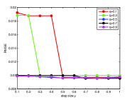
(a) Recovery Error

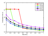
(b) Computational Time

Figure 1: Experiment for the justification of the effect of stepsize parameter $\mu$ on the performance of the CCD algorithm with different $q$. (a) The trends of recovery error of the CCD algorithm with different $q$. (b) The trends of the computational time of the CCD algorithm with different $q$.

V Conclusion

We propose a cyclic coordinate descent (CCD) algorithm for the non-convex $l_{q}$ ($0<q<1$) regularization problem. The main contribution of this paper is the establishment of the convergence analysis of the proposed CCD algorihm. In summary, we have verified that

1. the proposed CCD algorithm converges to a stationary point as long as $0<\mu<\frac{1}{L_{\max}}$ with $L_{\max}=\max_{i}\|A_{i}\|_{2}^{2}$, which is weaker than the convergence condition for the iterative jumping thresholding (IJT) algorithm applied to $l_{q}$ regularization with $0<\mu<\|A\|_{2}^{-2}$ [21]. This coincides with the common sense because the CCD algorithm proposed in this paper can be viewed as a Gauss-Seidel type algorithm while IJT algorithm can be seen as a Jocobi type algorithm.

2. the CCD algorithm further converges to a local minimizer of $l_{q}$ regularization if the regularization parameter $\lambda$ is relatively small.

Compared with the tightly related work in [23], there are two significant improvements. On one hand, we get rid of the column-normalization requirement of the measurement matrix $A$ via introducing a stepsize parameter that improves the flexibility and applicability of the CCD algorithm. In addition, the proposed CCD algorithm has almost the same performance of the $l_{q}$CD algorithm as demonstrated by the numerical experiments. On the other hand and also the more important one, we can justify the convergence of the proposed CCD algorithm by introducing the stepsize parameter. While only the subsequential convergence of $l_{q}$CD algorithm can be claimed in [23].

References

- [1] D. L. Donoho, Compressed sensing. IEEE Transactions on Information Theory, 52(4): 1289-1306, 2006.
- [2] E. J. Cands, J. Romberg, and T. Tao, Robust uncertainty principles: exact signal reconstruction from highly incomplete frequency information. IEEE Transactions on Information Theory, 52(2): 489-509, 2006.
- [3] M. Lustig, D. L. Donoho, J. M. Santos, and J. M. Pauly, Compressed sensing MRI, IEEE Signal Processing Magazine, 25:72-82, 2008.
- [4] M. F. Duarte and Y. C. Eldar, Structured compressed sensing: From theory to applications. IEEE Transactions on Signal Processing, 59: 4053-4085, 2011.
- [5] R. Tibshirani, Regression shrinkage and selection via the lasso, J. Royal Stat. Soc. Ser. B, vol. 58: 267-288, 1996.
- [6] B. A. Olshausen and D. J. Field, Emergence of simple-cell receptive field properties by learning a sparse code for natural images, Nature, vol. 381: 607-609, 1996.
- [7] P. Combettes and V. Wajs, Signal recovery by proximal forward-backward splitting. Multiscale Model. Simul., 4: 1168-1200, 2005.
- [8] J. Zhu, S. Rosset, T. Hastie and R. Tibshirani, 1-norm support vector machines, Neural Information Processing Systems (NIPS), 2003.
- [9] J. S. Zeng, J. Fang and Z. B. Xu, Sparse SAR imaging based on regularization, Science in China Series F-Information Science, 55: 1755-1775, 2012.
- [10] J. S. Zeng, Z. B. Xu, B. C. Zhang, W. Hong and Y. R. Wu. Accelerated regularization based SAR imaging via BCR and reduced Newton skills. Signal Processing, 93: 1831-1844, 2013.
- [11] B. K. Natarajan, Sparse approximate solutions to linear systems. SIAM J. Comput., 24: 227-234, 1995.
- [12] E. J. Cands, M. B. Wakin and S. P. Boyd, Enhancing sparsity by reweighted minimization, Journal of Fourier Analysis and Applications, 14 (5): 877-905, 2008.
- [13] R. Chartrand, Exact reconstruction of sparse signals via nonconvex minimization. IEEE Signal Processing Letters, 14 (10): 707-710, 2007.
- [14] R. Chartrand and V. Staneva, Restricted isometry properties and nonconvex compressive sensing, Inverse Problems, 24: 1-14, 2008.
- [15] D. Geman and G. Reynolds, Constrained restoration and the recovery of discontinuities, IEEE Transactions on Pattern Analysis and Machine Intelligence, 14 (3): 367-383, 1992.
- [16] D. Geman and C. Yang, Nonlinear image recovery with Half-Quadratic regularization, IEEE Transactions on Image Processing, 4 (7): 932 - 946, 1995.
- [17] I. F. Gorodnitsky and B. D. Rao, Sparse signal reconstruction from limited data using FOCUSS: a re-weighted minimum norm algorithm, IEEE Transactions on Signal Processing, 45 (3): 600-616, 1997.
- [18] G. Gasso, A. Rakotomamonjy and S. Canu, Recovering sparse signals with a certain family of nonconvex penalties and dc programming, IEEE Transactions on Signal Processing, 57(12): 4686 - 4698, 2009.
- [19] K. Bredies, and D. A. Lorenz, Minimization of non-smooth, non-convex functionals by iterative thresholding, http://citeseerx.ist.psu.edu /viewdoc/sum mary?doi=10.1.1.156.9058, 2009.
- [20] Z. B. Xu, X. Y. Chang, F. M. Xu and H. Zhang, regularization: a thresholding representation theory and a fast solver, IEEE Transactions on Neural Networks and Learning Systems, 23: 1013-1027, 2012.
- [21] J. S. Zeng, S. B. Lin and Z. B. Xu, Sparse Regularization: Convergence of Iterative Jumping Thresholding Algorithm, arXiv preprint arXiv:1402.5744, 2014.
- [22] P. Tseng, Convergence of block coordinate descent methods for non-differentiable minimization, J. Optimization Theory Appl., 109: 475-494, 2001.
- [23] G. Marjanovic, and V. Solo, sparsity penalized linear regression with cyclic descent, IEEE Transactions on Signal Processing, 62(6): 1464-1475, 2014.
- [24] R. Chartrand and Wotao Yin, Iterative reweighted algorithms for compressed sensing, IEEE international conference on Acoustics, speech and signal processing (ICASSP), 3869-3872, 2008.
- [25] I. Daubechies, R. Devore, M. Fornasier and C. S. Gunturk, Iteratively reweighted least squares minimization for sparse recovery, Communications on Pure and Applied Mathematics, 63: 1-38, 2010.
- [26] T. Zhang, Analysis of multi-stage convex relaxation for sparse regularization. Journal of Machine Learning Research, 11: 1081-1107, 2010.
- [27] I. Duabechies, M. Defrise, C. Mol, An iterative thresholding algorithm for linear inverse problems with a sparse constraint, Communications on Pure and Applied Mathematics, 57: 1413-1457, 2004.
- [28] T. Blumensath and M. E. Davies, Iterative thresholding for sparse approximation. Journal of Fourier Analysis and Application, 14(5): 629-654, 2008.
- [29] H. Attouch, J. Bolte and B. F. Svaiter, Convergence of descent methods for semi-algebraic and tame problems: proximal algorithms, forward-backward splitting, and regularized Gauss-Seidel methods. Math. Program., Ser. A, 137:91-129, 2013.
- [30] Y. T. Qian, S. Jia, J. Zhou and A. Robles-Kelly, Hyperspectral unmixing via sparsity-constrained nonnegative matrix factorization, IEEE Transactions on Geoscience and Remote Sensing, 49 (11): 4282-4297, 2011.
- [31] J.H. Friedman, T. Hastie, H. Hofling, and R. Tibshirani, Pathwise coordinate optimization, Ann. Appl. Stat., 1(2): 302-332, 2007.
- [32] R. Mazumder, J. H. Friedman, and T. Hastie, Sparsenet: Coordinate descent with nonconvex penalties, J. Amer. Statist. Assoc., 106: 1125-1138, 2007.
- [33] J. V. Burke, Descent methods for composite nondifferentiable optimization problems, Math. Program., 33: 260-279, 1985.
- [34] J. S. Zeng, S. B. Lin, Y. Wang and Z. B. Xu, Regularization: convergence of iterative half thresholding algorithm, IEEE Transactions on Signal Processing, 62(9): 2317-2329, 2014.
- [35] W. F. Cao, J. Sun, and Z. B. Xu, Fast image deconvolution using closed-form thresholding formulas of () regularization. Journal of Visual Communication and Image Representation, 24(1): 1529-1542, 2013.
- [36] A.M. Ostrowski, Solutions of equaltions in Euclidean and Banach spaces, New York, NY, USA: Academic, 1973.