Answering Regular Path Queries on Workflow Provenance

Abstract

This paper proposes a novel approach for efficiently evaluating regular path queries over provenance graphs of workflows that may include recursion. The approach assumes that an execution $g$ of a workflow $G$ is labeled with query-agnostic reachability labels using an existing technique. At query time, given $g$, $G$ and a regular path query $R$, the approach decomposes $R$ into a set of subqueries $R_{1}$, …, $R_{k}$ that are safe for $G$. For each safe subquery $R_{i}$, $G$ is rewritten so that, using the reachability labels of nodes in $g$, whether or not there is a path which matches $R_{i}$ between two nodes can be decided in constant time. The results of each safe subquery are then composed, possibly with some small unsafe remainder, to produce an answer to $R$. The approach results in an algorithm that significantly reduces the number of subqueries $k$ over existing techniques by increasing their size and complexity, and that evaluates each subquery in time bounded by its input and output size. Experimental results demonstrate the benefit of this approach.

I Introduction

Capturing and querying workflow provenance is increasingly important for scientific as well as business applications. By maintaining information about the sequence of module executions used to produce data, as well as the parameter settings and intermediate data passed between module executions, the validity and reproducibility of data can be enhanced.

A series of “provenance challenges”  was held between 2006 and 2010 to compare the expressiveness of various provenance systems. Many of the sample queries given in these challenges were simple reachability queries that check the existence of an (arbitrary) execution path between workflow nodes, e.g. “Identify the data sources that contributed some data leading to the production of publication $p$”. However, others were more complex, requiring the path between nodes to have a certain shape.

Such constraints on the path structure can naturally be captured by regular expressions. For example, the query “Find all publications $p$ that resulted from starting with data of type $x$, then performing a repeated analysis using either technique $a_{1}$ or technique $a_{2}$, terminated by producing a result of type $s$, and eventually ending by publishing $p$.” can be captured as the regular path query $R=\;x.(a_{1}|a_{2})^{+}.s.\_^{*}.p$.

As users become familiar with the power of provenance, such complex, regular path queries will become even more common. In particular, they are necessary to find workflows that exhibit certain types of behaviors within shared repositories of workflows and their executions, a topic of increasing interest within the scientific community [13, 27].

Answering regular path queries over graphs (in particular, XML trees) has been extensively studied [2, 9, 12, 28, 29, 30]. The typical approach used is to cut the query into smaller subqueries (e.g. reachability queries), and traverse the graph to answer each subquery. The results of the subqueries are then joined together to answer the original query. The problem with this approach is the large number and size of intermediate results, and the subsequent cost of joins. In this paper, we show that since workflow executions are not arbitrary graphs, but rather graphs that originate from a given specification, regular path queries can be processed much more efficiently. Specifically, we show that a regular path query does not need to be decomposed when it is safe for a given workflow specification. Safe queries are quite general, and go well beyond reachability queries.

Before discussing our solution, note that regular path queries, such as the one presented above, cannot be answered simply by looking at a workflow specification. This is because 1) the queries may involve run-time data; and 2) if the workflow specification contains alternatives then the exact paths between data may not be known in advance. For example, if a workflow specification $G$, which takes something of type $x$ as input, involves a choice of either executing $a_{1}$ repeatedly followed by $s$ and terminating with $p$ (which matches $R$), or executing $a_{3}$ repeatedly followed by $s$ and terminating with $p$ (which doesn’t match $R$), to answer the query one needs to examine which option was actually taken at run time. Nevertheless, we will see that the specification can still be used to speed up query processing.

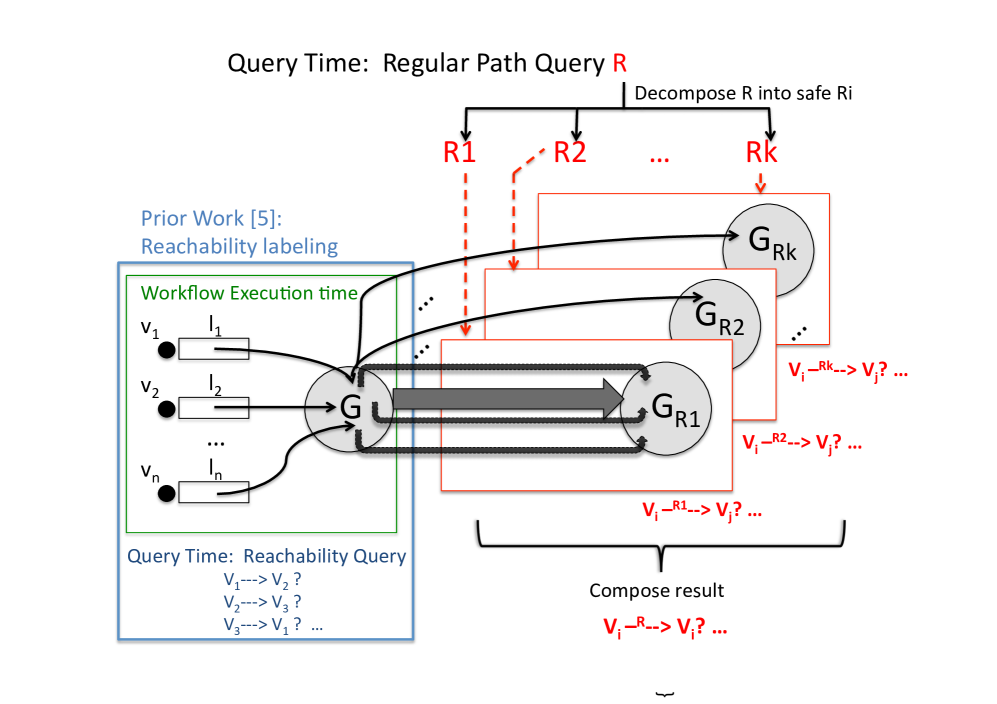
Figure 1: Overview of our approach

The approach we present in this paper, illustrated in Fig. 1, assumes that an execution $g$ of a workflow specification $G$ is labeled with query-agnostic, reachability labels using an existing technique [4] (left portion of Fig. 1; each $v_{i}$ is a node in $g$, and its reachability label $l_{i}$ references the specification $G$). At query time, given $g$, $G$ and a regular path query $R$, the approach decomposes $R$ into a set of subqueries $R_{1}$, …, $R_{k}$ which are safe for the specification $G$ . For each safe subquery $R_{i}$, $G$ is rewritten so that, using the reachability labels of nodes in $g$, whether or not there is a path which matches $R_{i}$ between two nodes $u$ and $v$ can be decided in constant time ($G_{R_{1}}$,…$G_{R_{k}}$ in Fig. 1). The results of each safe subquery are then composed, possibly with some small unsafe remainder, to produce an answer to $R$.

The reason this solution is possible is because the labeling in [4] is parameterized by the specification. The novelty in this paper is to rewrite the specification so that reachability labeling can be used to evaluate regular path expressions.

The benefit of this approach is 1) the number of subqueries is much smaller than previous approaches; 2) subqueries are larger and more complex than the atomic subqueries used previously, reducing the number and size of intermediate results; and 3) there are therefore fewer, potentially less expensive joins, hence overall a significant speedup is achieved. The type of executions (provenance graphs) for which this can be done are produced by a very general class of workflows expressed as context-free graph grammars [7], and which handle recursion in a reasonable way (strictly linear recursive [4]).

Related Work. The model of workflow provenance that we adopt in this paper is based on [14, 25]. The problem of labeling workflow runs to answer reachability queries was studied in [17], where they adapted the interval-based labeling for trees to work for DAGs. The problem with this approach is that the size of the transformed tree can be exponential in the size of the original DAG, which leads to linear-size interval labels. Furthermore, it does not extend to regular path queries since it is not parameterized by the specification.

Reachability queries have also been extensively studied for XML trees and graphs, and a common approach is to use labeling. An algorithm for all-pairs reachability queries over trees is given in [2], which executes in time linear in the input and output size and is therefore optimal. [9] gives an optimal algorithm for XML pattern matching. However, existing work on all-pairs reachability queries on DAGs/graphs cannot achieve linear time complexity  [12, 28, 29, 30].

Pairwise regular path queries on DAGs can be answered in time linear in graph size [24]. Two optimization techniques (query pruning and query rewriting) which use graph schemas [10] are proposed in [16]. [21] proposes to decompose regular expressions into concatenation/union/Kleene star subexpressions, and then uses reachability labeling to perform joins. Recently [20] proposes to use rare labels to decompose queries to smaller subqueries and perform a breadth-first search in parallel. [15] proposes multiple regular query variants and represents queries as datalog. [22] considers querying both data and the topology of graphs. [23] considers regular expressions with numerical occurrence indicators. Regular expressions of special forms have also been recently studied [19]. Languages for path queries over graph-structured data are surveyed in [6]; among them, [21, 24] [20] can be extended to our setting. We will show a comparison to this in the experiments.

Most relevant for this paper are the dynamic reachability labeling techniques of [3, 4, 5] for workflow provenance graphs, which address reachability queries between a single pair of nodes. In contrast, this paper addresses considerably more complex queries, regular path queries, between sets of nodes. To do this, we harness in a non-trivial way the labeling techniques in [4], and employ them for processing general queries over workflow provenance.

Contributions. In contrast to previous work, we answer regular path queries over graphs using labeling, by leveraging the fact that the graphs represent executions generated from a given workflow specification. Specifically:

$\bullet$ We identify a core property, safe query, that is defined for a query relative to a workflow specification, and that enables the use of reachability labels for processing regular path queries. We show that safety of a query can be detected in polynomial time in the size of the query and specification.

$\bullet$ Pairwise safe queries. We show how to rewrite a specification using a safe query $R$, and use the rewritten specification together with the reachability labels of two input nodes $u$ and $v$ to answer whether there exists a path between $u$ and $v$ which conforms to $R$ , $u\stackrel{{\scriptstyle R}}{{\leadsto}}v$, in constant time.

$\bullet$ All-pairs safe queries. We extend the pairwise query technique to answer all-pairs safe queries, which ask whether $u\stackrel{{\scriptstyle R}}{{\leadsto}}v$ for node pairs $(u,v)\in U\times V$, and give an algorithm for answering all-pairs queries that runs in time linear in $|U|,|V|,N$ and polynomial in the size of the specification, where $N$ is the number of reachable nodes in $U\times V$. As a side effect, we answer all-pairs reachability queries in linear time in the input and output size, which is optimal.

$\bullet$ All-pairs general queries. Finally, we present our approach for answering general regular path queries. We give a top-down algorithm for decomposing a general query into a small set of safe subqueries, and show how to compose results of the safe subqueries, possibly with some small unsafe remainder, to answer the original query.

$\bullet$ Experimental studies demonstrate the significant speedup that is achieved by our approach.

Outline. Section II presents the workflow model and reachability labeling of [4]. We formally define regular path queries, and discuss pairwise safe queries in Section III. In particular, we show how to transform a regular path query $R$ to a reachability query by rewriting the workflow specification and decoding the labels of nodes using the rewritten workflow; we also discuss conditions under which this can be done (safe query). Section IV shows how to answer all-pairs safe queries, and discusses how to decompose a general query into a small set of safe subqueries to answer general all-pairs queries. Experimental results are given in Section V.

II Prior Work

In this section, we summarize the workflow model and labeling scheme of [4]. Although the labeling scheme was designed to answer reachability queries, we will extend it in Section III to answer pairwise regular path queries.

II-A Workflow model [4]

A workflow specification is modeled as a context-free graph grammar (CFGG), which describes the design of the workflow and whose language corresponds to the set of all possible executions (runs). The model that we use is similar to [3, 7]. Nonterminals in a CFGG $G$ correspond to composite modules and terminals to atomic modules; edges in graphs in $G$ correspond to dataflow between modules. More formally, we start by defining simple workflows and build up to workflows using productions.

Definition 1

(Simple Workflow) A simple workflow is $W=(V,E)$, where $V$ is a set of modules and $E$ is a set of data edges between modules. Each node $v$ has a name drawn from a finite set of symbols $\Sigma$, denoted $name(v)$. Each edge $e$ is tagged with an element of a finite set of symbols, $\Gamma$, which represents the name of the data flowing over the edge, denoted $\tau_{E}(e)$. There may be multiple parallel edges between two nodes, each with a different tag.

Simple workflows are reused as composite modules to build more complex workflows. This is modeled using workflow productions.

Definition 2

(Workflow Production) A workflow production is of form $M\rightarrow W$, where $M$ is a composite module and $W$ is a simple workflow.

Definition 3

(Workflow Specification) A workflow specification is a CFGG $G=(\Sigma,\Delta,S,P)$, where $\Sigma$ is a finite set of modules, $\Delta\subseteq\Sigma$ is a set of composite modules (then $\Sigma\setminus\Delta$ is the set of atomic modules), $S\in\Sigma$ is a start module, and $P=\{M\rightarrow W\ |\ M\in\Delta,W\in\Sigma^{*}\}$ is a finite set of workflow productions (i.e. $W$ is a simple workflow whose nodes are modules in $\Sigma$). We will frequently refer to workflow specifications as workflows.

Definition 4

(Workflow Derivation and Execution) A given workflow execution is derived by a series of node replacements or derivation steps corresponding to the productions in the specification. We start with a graph $g_{0}$ consisting of a node named $S$. At the $i^{th}$ step of the derivation, a new graph $g_{i}$ is obtained by replacing (executing) some composite node $v$ of the current graph $g_{i-1}$ with a simple workflow $W$, where $p:name(v)\rightarrow W$ is a production of the grammar. If $u$ is a node in $W$, then we say that $v$ derives $u$ ($u$ is derived by $v$) and extend this transitively. We denote by $(v,p)$ a node replacement. The language of a workflow is the set of all executions.

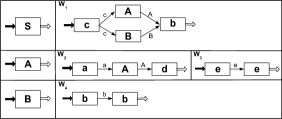
(a) Workflow specification $G$

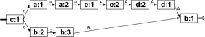
(b) A run of $G$

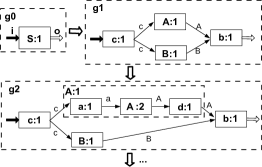
(c) Partial derivation graph

Figure 2: Sample Workflow

To simplify, in the examples of specifications throughout this paper the tags on edges are the same as the name of the modules at their head.

Example II.1

An example of a workflow specification is shown in Fig. 2a, and one of its runs in Fig. 2b. Upper case module names ($S$, $A$, $B$) correspond to composite modules, and lowercase to atomic modules ($a$, $b$, $c$, $d$, $e$). The specification contains a choice of implementations for $A$, i.e. either $W_{2}$ or $W_{3}$. The run inherits node (module) names and edge tags from its specification; to disambiguate multiple occurrences of the same module an occurrence number is appended to module names to form a unique node id. A partial sequence of derivation steps that would arrive at the run is shown in Fig. 2c. We start with a graph $g_{0}$ consisting of a single node $S:1$.In the first step, we replace $S:1$ with $W_{2}$; $S:1$ therefore derives $c:1$, $A:1$, $B:1$ and $b:1$ since they are nodes in $W_{2}$. Similarly, in the second step, we replace $A:1$ by $W_{2}$; $A:1$ therefore derives $a:1$, $A:2$ and $d:1$. By transitivity, $S:1$ also derives $a:1$, $A:2$ and $d:1$.

In a fine-grained workflow model, each module $M$ may have multiple input/output ports, each representing a different data item. Explicit dependencies between the output of an atomic module and a subset of its inputs can be captured as internal module edges. For example, if an atomic $m$ has two inputs, $x$ and $y$, and produces as output $x$ and $x+y$, $m$ would have two input ports and two output ports (see Fig. 3). The first output port, representing $x$, would be connected only to the first input port, representing $x$, while the second output port, representing $x+y$, would be connected to both input ports. The dependency between input and output ports of a composite module may vary according to its execution (more details can be found in Section II-B). Executions of fine-grained workflows are also fine-grained.

Figure 3: Fine-grained workflow

II-B Reachability labeling [4]

The labeling scheme in [4], called dynamic, derivation based labeling, was designed to answer reachability queries over views of workflows. A reachability query is one which, given two nodes $u$, $v$ in a run $g$, returns “yes” iff there is a path from $u$ to $v$ in $g$ (written $u\leadsto v$). The labeling scheme is based on the fine-grained workflow model; however, it labels a run as if the workflow were coarse-grained, encoding only the sequence of productions used to arrive at each node (hence the name derivation-based). Reachability queries over views are then answered by decoding the labels using the fine-grained workflow specification intersected with the view definition. In a similar way, to answer regular path queries we label a run as if it were coarse-grained; however, to decode labels we will use the query intersected workflow specification $G_{R}$, which is fine-grained. Readers familiar with the results in  [4] can go directly to Section III.

Constraints. A labeling scheme is optimal (or compact) if 1) labels are logarithmic in the size of the run, and 2) labels can be decoded in constant time, assuming that any operation on two words ($log\;n$ bits) can be done in constant time. For compact reachability labeling to be achievable for fine-grained workflows, two corresponding constraints must be met: 1) the workflow must be strictly-linear recursive; and 2) the workflow must be safe. The first condition is essential for logarithmic-size labeling and the second for efficient decoding.

To define the first constraint, we use the notion of a production graph.

Definition 5

(Production Graph) Given a workflow $G=(\Sigma,\Delta,S,P)$, the production graph of $G$ is a directed multigraph ${\cal P}(G)$ in which each vertex denotes a unique module in $\Sigma$. For each production $M\rightarrow W$ in $P$ and each module $M^{\prime}$ in $W$, there is an edge from $M$ to $M^{\prime}$ in ${\cal P}(G)$. Note that if $W$ has multiple instances of a module $M^{\prime}$, then ${\cal P}(G)$ has multiple parallel edges from $M$ to $M^{\prime}$.

Definition 6

(Strictly Linear-Recursive Workflow) A workflow $G$ is recursive if ${\cal P}(G)$ is cyclic, and a module in $G$ is recursive if it belongs to a cycle in ${\cal P}(G)$. $G$ is strictly linear-recursive iff all cycles in ${\cal P}(G)$ are vertex-disjoint.

Example II.2

The production graph for the grammar $G$ in Fig. 2a is shown in Fig. 5 (ignore for now the pair of numbers on edges). $G$ is recursive since there is a cycle in ${\cal P}(G)$; it is strictly linear-recursive since ${\cal P}(G)$ contains only one cycle. The only recursive node in $G$ is $A$.

In contrast, the hypothetical (and unlabeled) production graph shown in Fig. 5 contains two cycles which share a node, $S$, and therefore the workflow that it represents is not strictly linear-recursive.

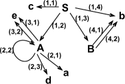
Figure 4: Production graph ${\cal P}(G)$

Figure 5: Synthetic production graph

As argued in [4], strict linear recursion is able to capture common recursive patterns found in repositories of scientific workflows, in particular looping and forked executions.

Now we turn to the second constraint. Recall that a fine-grained workflow is such that each atomic module has one or more input/output ports whose dependency is explicitly specified by module internal edges (see Fig. 3). The dependency between the input and output ports of a composite module is determined by the executions of the module. Intuitively, if a workflow is safe, we can draw unambiguous internal edges for all composite modules.

Definition 7

(Safe Workflow) A workflow $G$ is safe iff for each composite module, the dependency between its input and output ports is deterministic w.r.t. all its executions.

Example II.3

Consider the fine-grained workflow below and two of its executions $ex_{1}$ and $ex_{2}$. In $ex_{1}$, the second output port of $S$ solely depends on the second input port of $S$. However, in $ex_{2}$, the second output port of $S$ depends on both input ports of $S$. Thus the dependency between the input and output ports of $S$ is not deterministic. Therefore the workflow is not safe. An example of safe workflow is given in Fig. 9, where the dependency for composite modules are illustrated by internal module edges.

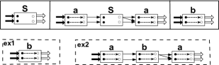
Figure 6: Unsafe workflow

Labeling $\psi_{V}(u)$. The labeling function $\psi_{V}$ assigns a label to each node $u$ when the node is derived and will not change the label as the workflow is executed. The approach is based on a tree representation for a run, called the compressed parse tree. In contrast to the traditional parse tree used for context-free grammars whose depth may be proportional to the size of the run, the depth of a compressed parse tree is bounded by the size of the specification. The compressed parse is constructed in a top-down manner, i.e. as productions are fired. A label is assigned to each node (module execution) as soon as it is executed, and encodes the sequence of derivation steps that create the module.

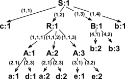
Figure 7: Compressed Parse Tree

Example II.4

The compressed parse tree for the run in Fig. 2b is shown in Fig. 7 (ignore the tree edge labels for now). Each leaf node denotes an atomic module, and each non-leaf node denotes either a composite module or a linear recursion, called a recursive node and labeled $R$. The children of a composite node denote the modules of the simple workflow produced by the production used in its execution; and the children of a recursive node denote a sequence of nested composite modules obtained by unfolding a cycle in the production graph. As before, occurrence numbers are used to disambiguate module executions. In the sample run, $A$ is executed three times (denoted $A:1$, $A:2$, $A:3$), twice using $W_{2}$ and the final time using $W_{3}$.

Edges in the compressed parse tree $T$ are labeled as follows (we denote by $\psi_{T}(e)$ the label of an edge $e$): We begin with assigning labels to edges of the production graph of the specification, ${\cal P}(G)$ . First of all, fix an arbitrary ordering among the productions in $P$, and for each production $M\rightarrow W$, fix an arbitrary topological ordering among the modules in $W$. Let $p_{k}=M\rightarrow W$ be the $k$th production in $P$, and $M_{i}$ be the $i$th module in $W$, then we assign the edge from $M$ to $M_{i}$ in ${\cal P}(G)$ a pair $(k,i)$. In addition, fix an arbitrary ordering among all the cycles in ${\cal P}(G)$, and for each cycle, fix an arbitrary edge as the first edge of the cycle. We are now ready to label $T$. Let $e=(u,v)$ be an edge of $T$. (1) If $u$ is a composite node, then $e$ can be mapped to an edge $e^{\prime}$ in ${\cal P}(G)$. Let $e^{\prime}=(k,i)$, then $\psi_{T}(e)=(k,i)$; and (2) otherwise (if $u$ is a recursive node), let $u$ denote the $s$th cycle in ${\cal P}(G)$ starting from the $t$th edge. Let $v$ be the $i$th child of $u$, then $\psi_{T}(e)=(s,t,i)$.

Example II.5

Consider ${\cal P}(G)$ shown in Fig. 5. The productions are ordered as shown in the Fig. 2a. For example, the edge between $S$ and $c$ is labeled (1,1) since $W_{1}$ is the first production, and $c$ is chosen as the first module in its body. The edge labels for Fig. 7 were constructed as follows: Labels on edges from the root $S$ of $T$ were taken from the production graph in Fig. 5. Since there is only one cycle in ${\cal P}(G)$ it is the first cycle, and its first (and only) edge is (2,2). Thus the cycle is labeled (1,1). The children of the recursive node $R$ were ordered by their order of execution. Thus we label edge $(R:1,A:2)$ in $T$ as (1,1,2), meaning that $A:2$ is the second child of $R:1$ which corresponds to the first cycle in ${\cal P}(G)$ starting from the first edge.

A module execution (node $v$ in $T$) is labeled using the concatenation of edge labels from the root of $T$ to $v$, denoted by $\psi_{V}(v)$. For example, $\psi_{V}(b:2)=(1,3)(4,1)$.

Decoding $\pi(\psi_{V}(u),\psi_{V}(v),G)$. Given a pair of module executions $u$, $v$ in a run that was generated from the workflow $G$, the predicate $\pi(\psi_{V}(u),\psi_{V}(v),G)$ outputs whether $u$ is reachable to $v$ in the run. A constant-time algorithm to evaluate $\pi(\psi_{V}(u),\psi_{V}(v),G)$ is presented in [4]. The subtlety is that the workflow $G$ is taken as a parameter. As a very simple example, consider node $c:1$ and $b:1$ of the run in Fig. 8 which was derived from the (safe) workflow in Fig. 9. Once we know $c:1$ and $b:1$ are from the same node replacement i.e. $(S:1,S\rightarrow W_{1}^{\prime})$ (which is determined by identifying their least common ancestor in the compressed parse tree (Fig. 7) using their labels), we know directly from $W_{1}^{\prime}$ the connectivity between $c:1$ and $b:1$. This is done in constant time because we access the specification rather than the run. Details of the decoding algorithm are omitted here, since they are not necessary for understanding the new techniques that will be proposed in this work.

III Answering Pairwise Safe Queries

In this section, we show how to answer pairwise safe queries, assuming that the execution has been labeled using the reachability labeling scheme of [4]. To achieve this, we must do two things: 1) reduce regular path queries to equivalent reachability queries; and 2) identify constraints on $G$ and $R$ which allow reachability labeling to be used.

Informally, our approach works as follows. We reduce regular path queries on a coarse-grained workflow $G$ to equivalent reachability queries on a fine-grained (and query-specific) workflow $G_{R}$. This workflow is obtained by intersecting $G$ with a DFA of query $R$, thereby modeling DFA state transitions within modules of $G_{R}$ while leaving the sequence of productions unchanged (Section III-B). Since reachability labeling only works for safe workflows, we discuss in Section III-C a class of safe queries which guarantee that the query-intersected workflow $G_{R}$ is safe. Since the run $g$ is labeled with information about the sequence of productions used as it was executed, the (pre-existing) reachability labels of a pair of nodes $u$, $v$ can then be combined at query time with DFA state transition information in $G_{R}$ to answer $u\stackrel{{\scriptstyle R}}{{\leadsto}}v$ (Section III-D).

We start in Section III-A by formally defining the class of queries studied in this paper.

III-A Regular path queries

To simplify the presentation, in this paper we will consider regular path queries on coarse-grained workflows in which each module has a single-input and single-output, and the output is assumed to depend on the input; we also assume that simple workflows are acyclic.

Queries are regular expressions over edge tags, defined using concatenation, alternation and Kleene star:

$$e~{}:=~{}c~{}|~{}e_{1}e_{2}~{}|~{}e_{1}+e_{2}~{}|~{}e_{1}^{*}~{}|~{}e_{1}^{+}$$

where $c~{}:=~{}\epsilon~{}|~{}\_~{}|~{}a$ is a constant regular expression ($\epsilon$ is the empty string and $~{}\_~{}$ is the wildcard symbol that matches any single symbol); $e_{1}e_{2}$ denotes the concatenation of two sub-expressions; $e_{1}+e_{2}$ denotes alternation; and $e_{1}^{*}$ ($e_{1}^{+}$) denotes the set of all strings that can be obtained by concatenating zero (one) or more strings chosen from $e_{1}$. Given a regular expression $R$, we denote by $L(R)$ the set of strings that conform to $R$.

Definition 8

(Regular Path Query) Let $G$ be a workflow specification and $g\in L(G)$ be a run. Given a path $p=v_{0}\xrightarrow{e_{1}}v_{1}\xrightarrow{e_{2}}v_{2}\ldots v_{n-1}\xrightarrow{e_{n}}v_{n}$ in $g$, we define $\tau_{P}(p)$ to be the concatenation of all edge tags on this path, that is, $\tau_{P}(p)=\tau_{E}(e_{1})\tau_{E}(e_{2})\ldots\tau_{E}(e_{n})\in\Gamma^{*}$. A regular path query $R$ over $g$ is a regular expression over $\Gamma$. The result of $R$ on $g$ is defined as the set of node pairs $(u,v)$ in $g$ such that there is a path $p$ in $g$ from $u$ to $v$ where $\tau_{P}(p)\in L(R)$.

In this paper, we study two related sub-problems of answering regular path queries over workflow runs, pairwise queries and all-pairs queries.

Definition 9

(Pairwise Query) Given two nodes $u,v$ from an edge-tagged graph $g$, a pairwise query $R$ asks if there exists a path $p$ from $u$ to $v$ in $g$ such that $\tau_{P}(p)\in L(R)$, denoted by $u\stackrel{{\scriptstyle R}}{{\leadsto}}v$.

The answer to a pairwise query is either true or false; reachability is a special case ($R=\;\_^{*}$).

Definition 10

(All-Pairs Query) Given two lists of nodes $l_{1},l_{2}$ from an edge-tagged graph $g$, all-pairs query $R$ asks for all node pairs $(u,v)\in l_{1}\times l_{2}$ such that $u\stackrel{{\scriptstyle R}}{{\leadsto}}v$.

Example III.1

Let $R_{1}=\;A^{+}$ and $R_{2}=\;A$. Revisiting the run in Fig. 2b, the pairwise query result of $R_{1}$ for $(d:2,b:1)$ is true, but is false for $R_{2}$. The all-pairs query result of $R_{1}$ for $l_{1}=\{d:1,d:2,e:2\}$, $l_{2}=\{b:1,b:2\}$ is $\{(d:1,b:1),(d:2,b:1),(e:2,b:1)\}$. The all-pairs query result of $R_{2}$ for $l_{1}$, $l_{2}$ is $\{(d:1,b:1)\}$.

In the next subsection, we reduce regular path queries on coarse-grained workflows to reachability queries on fine-grained workflows.

III-B From regular path queries to reachability queries

A simple algorithm for answering a pairwise regular path query $R$ over a run $g\in L(G)$ works as follows: augment each module in the run with input and output ports representing the states of a DFA for $R$, and connect the output port of module execution $u$ representing state $q$ to the input port of module execution $v$ representing state $q^{\prime}$ iff the tag of edge $e=(u,v)$ causes the DFA to transition from $q$ to $q^{\prime}$ ($\delta(q,\tau_{E}(e))=q^{\prime}$). Atomic modules leave states unchanged. Then for any two nodes $u,v$ in $g$, $u\stackrel{{\scriptstyle R}}{{\leadsto}}v$ iff the input port of $u$ representing the start state of the DFA reaches an output port of $v$ representing an accepting state of the DFA. This algorithm is linear in the run size since it needs to scan the run to perform the intersection.

Example III.2

The fine-grained run in Fig. 8 corresponds to the sample run in Fig. 2b, augmented with state transition information for query $R_{3}$ (Fig. 11a). Since there are two states in the DFA for $R_{3}$ , $q_{0}$ and $q_{f}$, each module execution has two input ports and two output ports. Since there is an edge tagged $e$ between $e:1$ and $e:2$ in the sample run, the output port $q_{0}$ of $e:1$ connects to the input port $q_{f}$ of $e:2$. All other edge tags leave the DFA in the same state.

In the sample run, $R_{3}=(\_)^{*}e(\_)^{*}$ evaluates to true for $(c:1,b:1)$, but false for $(c:1,b:3)$. Correspondingly, in the fine-grained run there is a path from the input port $q_{0}$ of $c:1$ to the output port $q_{f}$ of $b:1$, but there is no path from the input port $q_{0}$ of $c:1$ to the output port $q_{f}$ of $b:3$.

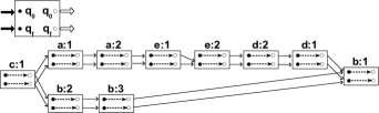
Figure 8: Fine-grained representation of sample run for query $R_{3}$

However, since the run is very large compared to the specification, we do not actually want to generate the query-augmented run. Rather, we augment the workflow specification with state-transition information from the DFA for $R$, transforming $G$ into a query-specific, fine-grained workflow. We then use the derivation information encoded as labels in the run to answer pairwise queries.

We now describe how to augment the workflow specification with DFA state-transition information by intersecting the workflow with the DFA.

Let ${\cal M}=(Q,\Gamma,\delta,q_{0},F)$ be a DFA of query $R$. We intersect the specification $G=(\Sigma,\Delta,S,P)$ with $\cal M$ to obtain a new specification $G_{R}=(\Sigma^{\prime},\Delta^{\prime},S^{\prime},P^{\prime})$ as follows:

1. For each module $M\in\Sigma$, create an augmented module $f_{M}(M)$ in $\Sigma^{\prime}$, where $f_{M}(M)$ has $|Q|$ input ports $I_{1}\ldots I_{|Q|}$ and $|Q|$ output ports $O_{1}\ldots O_{|Q|}$, corresponding to the $|Q|$ states of $\cal M$. Module names are preserved, i.e. $name(f_{M}(M))=\;name(M)$. For each atomic module $M\in\Sigma/\Delta$, for each input port $q$ of $M$, there is an edge from $q$ to the output port $q$ of $M$.

2. For each $M\in\Delta$, add $f_{M}(M)$ to $\Delta^{\prime}$. $S^{\prime}=\;f_{M}(S)$.

3. For each production $p:M\rightarrow W\in P$ where $W=(V,E)$, construct a new production $f_{P}(p):f_{M}(M)\rightarrow W^{\prime}\in P^{\prime}$, where $W^{\prime}=(V^{\prime},E^{\prime})$ is constructed from $W$ by (i) for each $v\in V$, $f_{M}(v)\in V^{\prime}$; and (ii) for each edge $e=(u,v)\in E$ there is an edge from output port $q$ of $f_{M}(u)$ to input port $q^{\prime}$ of $f_{M}(v)$ iff $\delta(q,\tau_{E}(e))=q^{\prime}$.

Example III.3

The intersection of the specification $G$ of Fig. 2a and the query $R_{3}=\_^{*}e\_^{*}$ in Fig. 11a is shown in Fig. 9 (ignore the edges inside composite modules for now). Each module in $G_{R}$ has two input ports and two output ports corresponding to $q_{0}$ and $q_{f}$. The only occurrence of the edge tag $e$ in $G$ is on the edge $(e,e)$ in $W_{2}$. Since $\delta(q_{0},e)=q_{f}$, $\delta(q_{f},e)=q_{f}$, all output ports of the first $e$ in $W^{\prime}_{2}$ are connected to the $q_{f}$ input port of the second $e$. All other augmented modules in $G_{R}$ connect $q_{0}$ to $q_{0}$ and $q_{f}$ to $q_{f}$.

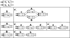
Figure 9: The fine-grained grammar $G_{R}$ obtained by intersecting $G$ with query $R_{3}$

We now reduce a pairwise query $R$ over a run $g$ generated by $G$ into an equivalent reachability query over a run $g^{\prime}$ generated by $G_{R}$. The correctness is shown below.

Lemma III.1

Let $G$ be a workflow, $\cal M$ be a DFA for query $R$, and $G_{R}$ be the intersection of $G$ with $\cal M$. Given any two vertices $u,v$ of $g\in L(G)$, $u\stackrel{{\scriptstyle R}}{{\leadsto}}v$ iff the $q_{0}$ input port of $u$ reaches an accepting output port $q_{f}$ of $v$ in $g^{\prime}$, where $g^{\prime}\in L(G_{R})$ is the run obtained by the same sequence of node replacements as $g$.

Proof:

Let $G_{R}=(\Sigma^{\prime},\Delta^{\prime},S^{\prime},P^{\prime})$ be the intersection of $G=(\Sigma,\Delta,S,P)$ and ${\cal M}=(Q,\delta,q_{0},F)~{}$, and $g$ be a run of $G$ derived by the sequence of node replacement $(v_{1},p_{1})\ldots(v_{n},p_{n})$. Note that $f_{M},f_{P}$ are bijective functions. The corresponding run $g^{\prime}\in G_{R}$ is derived by the sequence of node replacements $(v_{1}^{\prime},f_{P}(p_{1}))\ldots(v_{n}^{\prime},f_{P}(p_{n}))$. Observe that since $g$ and $g^{\prime}$ are derived by corresponding sequences of node replacements, the only difference between $g$ and $g^{\prime}$ is the addition of input/output ports and connections between modules corresponding to edge tag induced state transitions in the DFA.

If $u\stackrel{{\scriptstyle R}}{{\leadsto}}v$ in $g$, then there is a path $p=e_{1}...e_{k}$ from $u$ to $v$ in $g$ with $e_{i}=(u_{i-1},u_{i})$ ($u=u_{0}$ and $v=u_{k}$) such that $\delta(q_{0},\tau_{E}(e_{1}))=q_{1}$, $\delta(q_{1},\tau_{E}(e_{2}))=q_{2}$, …, $\delta(q_{k-1},\tau_{E}(e_{k}))=q_{f}$, and $q_{f}$ is a final state in ${\cal M}$. Thus there are corresponding edges $e^{\prime}_{i}$ in $g^{\prime}$ from output port $q_{i-1}$ of $u^{\prime}_{i-1}$ to input port $q_{i}$ of $u^{\prime}_{i}$. Since modules in $g^{\prime}$ are atomic, the $i$’th input port of each module is connected to its $i$’th output port. Hence there is a path $p^{\prime}$ in $g^{\prime}$ from input port $q_{0}$ in $u^{\prime}$ to output port $q_{f}$ in $v^{\prime}$. The only-if direction proceeds analogously. ∎

The benefit of this approach is that intersecting the workflow $G$ with a DFA $\cal M$ to obtain $G_{R}$ models state transitions in $\cal M$ but does not change the sequence of productions in $G$. Thus the reachability labels of [4], which rely solely on the production sequence that arrive at a node, can be used. However, in order to use the results of [4] $G_{R}$ must be 1) strictly-linear recursive, a condition which is guaranteed by $G$ being strictly-linear recursive; and 2) safe, a condition which is guaranteed by $R$ being a safe query for $G$. We next discuss the general problem of using (dynamic) labels for answering regular path queries, and then define safe queries.

III-C Safe Queries

Due to the complexity of regular expressions, there are specifications for which dynamic labeling is not possible, even if arbitrarily large labels are allowed. For example, consider the grammar in Fig. 2a and query $(\_)^{*}a(\_)^{*}$. At the second step of the derivation of the run in Fig. 2b, the graph $g_{1}$ is $W_{1}$. Observe that we cannot tell if the query will be satisfied for ($c:1$, $b:1$), and therefore it is impossible to label them as they arise: If $A\rightarrow W_{2}$ is applied, the answer would be “yes”. However, if $A\rightarrow W_{3}$ is applied, the answer would be “no”. We therefore say that query $(\_)^{*}a(\_)^{*}$ is not safe with respect to this workflow. In contrast, the query $(\_)^{*}e(\_)^{*}$ is safe, since $A$ must eventually terminate with an execution of $W_{3}$. It is also easy to see that the reachability query $(\_)^{*}$ is safe with respect to any workflow, since every module in a coarse-grained model has a single input and a single output.

We formally define safety of a query with respect to a workflow in terms of a finite state automata (DFA) for the query. Since there may be several equivalent DFAs for a query, we then show that it is sufficient to consider the minimal DFA for the query, and give an efficient algorithm for checking safety using the minimal DFA.

Recall the standard definition of a DFA [18]:

Definition 11

(DFA) A DFA ${\cal M}$ is a 5-tuple $(Q,\Gamma,\delta,q_{0},F)$, where $Q$ is a set of states, $\Gamma$ is a set of input symbols (i.e., edge tags), $\delta:Q\times\Gamma\rightarrow Q$ is a transition function, $q_{0}$ is the start state and $F\subseteq Q$ is a set of accept states. We extend $\delta$ to $\delta^{*}:Q\times\Gamma^{*}\rightarrow Q$ such that $\delta^{*}(q,w_{1}\ldots w_{n})=\delta^{*}(\delta(q,w_{1}),w_{2}\ldots w_{n})$ where $w_{i}\in\Gamma$.

Definition 12

(Safe DFA) A DFA ${\cal M}=(Q,\Gamma,\delta,q_{0},F)$ is safe with respect to a workflow specification $G=(\Sigma,\Delta,S,P)$ iff any state pair $(q_{1},q_{2})\in Q\times Q$ is safe. A state pair $(q_{1},q_{2})$ is safe iff $\forall M\in\Sigma$ and any two executions $ex_{1},ex_{2}$ of $M$, if there exists a path $p$ connecting an input $i$ of $M$ and an output $o$ of $M$ in $ex_{1}$ such that $\delta^{*}(q_{1},\tau_{P}(p))=q_{2}$, then there exists a path $p^{\prime}$ connecting $i$ and $o$ in $ex_{2}$ such that $\delta^{*}(q_{1},\tau_{P}(p^{\prime}))=q_{2}$.

Definition 13

(Safe Query) A regular path query $R$ is said to be safe with respect to a workflow specification $G$ iff there exists a DFA that accepts $R$ and is safe with respect to $G$.

Example III.4

Consider the composite module $A$ in the sample workflow $G$ in Fig. 2a. Two of $A$’s executions are shown in Fig. 10; all other executions of $A$ will represent $k$ recursions, with $k$ modules named $a$, followed by two named $e$, followed by $k$ named $d$.

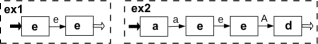
Figure 10: Two of $A$’s executions

(a) $R_{3}:(\_)^{*}e(\_)^{*}$ (safe)

(b) $R_{4}:e$ (not safe)

Figure 11: Two regular path queries

The DFAs of two queries are shown in Figures 11. $R_{3}$ is safe with respect to $G$ since all state pairs (i.e., $(q_{0},q_{0})$, $(q_{f},q_{f})$, $(q_{0},q_{f})$) are safe. For example, $(q_{0},q_{f})$ is safe because all executions of $S$ and $A$ contain a path whose tag transitions the DFA from $q_{0}$ to $q_{f}$, whereas none of $B$’s executions contains a path whose tag transitions the DFA from $q_{0}$ to $q_{f}$.

In contrast, $R_{4}$ is not safe with respect to $G$ because $(q_{0},q_{f})$ is not safe. In particular, the two executions of $A$ shown in Fig. 10, $ex_{1}$, $ex_{2}$, behave differently: There exists a path in $ex_{1}$ that transitions the DFA from $q_{0}$ to $q_{f}$, but there does not exist such a path in $ex_{2}$.

Note that the number of states of the DFA determines the size of the fine-grained workflow. We now show that it is sufficient to check the minimal DFA for $R$ in order to determine whether or not $R$ is safe for a given workflow.

Lemma III.2

Given a workflow $G$ and a regular expression $R$, $R$ is safe with respect to $G$ iff the minimal DFA of $R$ is safe with respect to $G$.

Proof:

By definition 13, it suffices to show that if the minimal DFA of $R$ is unsafe with respect to $G$ then all DFAs of $R$ are unsafe with respect to $G$. Specifically, for any unsafe state pair of the minimal DFA, we can always find in any DFA of $R$ a corresponding state pair that is unsafe.

Let ${\cal M}=(Q,\delta,q_{0},F)$ be any DFA of $R$, and $\\ {\cal M}_{min}=(Q_{min},\delta_{min},q^{min}_{0},F_{min})$ be the minimal DFA. By the definition of minimal DFA, for any state $q\in Q$ there is an equivalent state $q_{min}\in Q_{min}$, denoted by $q\equiv q_{min}$ (which we will define later) and vice versa. Suppose $(q_{1}^{min},q_{2}^{min})\in Q_{min}\times Q_{min}$ is unsafe with respect to some composite module $M$, i.e. there are two executions $W_{1},W_{2}$ of $M$ where there exists some path $p$ connecting the input $i$ and output $o$ of $M$ in $W_{1}$ such that

$$\delta^{*}_{min}(q_{1}^{min},\tau_{P}(p))=q_{2}^{min}$$ (1)

while for every path $p^{\prime}$ connecting $i$ and $o$ in $W_{2}$, $\\ \delta^{*}_{min}(q_{1}^{min},\tau_{P}(p^{\prime}))\not=q_{2}^{min}$. Now choose a state $q_{1}\in Q$ such that $q_{1}\equiv q_{1}^{min}$. Let

$$q_{2}=\delta^{*}(q_{1},\tau_{P}(p))$$ (2)

We prove that (1) $q_{2}\equiv q^{min}_{2}$ and thus $q_{2}$ is not a rejecting state; and (2) $(q_{1},q_{2})$ is unsafe w.r.t. $M$.

We first prove $q_{2}\equiv q^{min}_{2}$. Proof is by contradiction. Suppose $q_{2}\not\equiv q^{min}_{2}$. Recall from [18], a state $q$ of $\cal M$ is equivalent to a state $q_{min}$ of ${\cal M}_{min}$ iff any string that transits $\cal M$ from $q$ to some accepting state transits ${\cal M}_{min}$ from $q_{min}$ to some accepting state and vice versa. Formally $q\equiv q_{min}$ iff $\{w|\delta^{*}(q,w)\in F\}=\{w|\delta_{min}^{*}(q_{min},w)\in F_{min}\}$. Take any string $w$ that transits ${\cal M}_{min}$ from $q^{min}_{2}$ to some accepting state while cannot transit ${\cal M}$ from $q_{2}$ to some accepting state. Because of Equation 1, string $\tau_{P}(p)w$ transits ${\cal M}_{min}$ from $q^{min}_{1}$ to some accepting state while because of Equation 2, $\tau_{P}(p)w$ cannot transit $\cal M$ from $q_{1}$ to some accepting state, which contradicts $q_{1}\equiv q^{min}_{1}$.

We prove the second one by first showing that for any string $w$, if $q^{min}_{1}\equiv q_{1},q^{min}_{2}\equiv q_{2}$ and $\delta_{min}^{*}(q^{min}_{1},w)\not=q^{min}_{2}$, then $\delta^{*}(q_{1},w)\not=q_{2}$. Proof is similar to the first part. Recall that no path in $W_{2}$ can transit from $q^{min}_{1}$ to $q^{min}_{2}$. Thus no path in $W_{2}$ can transit from $q_{1}$ to $q_{2}$. Revisiting Equation 2, the path $p$ in $W_{1}$ can transit from $q_{1}$ to $q_{2}$. Thus by Definition 13, $(q_{1},q_{2})$ is unsafe. ∎

In the rest of the paper, we refer to the minimal DFA of a query as its DFA.

Checking safety of DFA: Intuitively, a DFA $\cal M$ is safe w.r.t. a workflow $G$ if the fine-grained workflow $G_{R}$ obtained by intersecting $G$ with $\cal M$ is safe. We must therefore understand the internal edges in modules of $G_{R}$, since a safe workflow is one in which the dependency between the input and output ports of each composite module is deterministic w.r.t. all its executions (recall Section II-B). An atomic module leaves states of a DFA unchanged; thus we draw an internal edge from the input port representing $q$ to the output port representing $q$. If the DFA $\cal M$ is safe, then internal edges can be “lifted” deterministically to composite modules.

Example III.5

Consider the internal module edges in Fig. 9. All atomic modules leave the state unchanged. The execution of composite module $B$ leaves the states unchanged, whereas any execution of composite module $A$ causes a transition from $q_{0}$ to $q_{f}$, and from $q_{f}$ to $q_{f}$. Thus $R_{3}$ is safe for $G$.

An algorithm for checking safety is as follows: We denote by $\lambda(M,ex)$ for each execution $ex$ of each module $M\in\Sigma$ a $|Q|\times|Q|$ boolean matrix, such that $\lambda(M,ex)[q_{1},q_{2}]=1$ iff there exists a path in $ex$ whose tag can transition the DFA from $q_{1}$ to $q_{2}$. Note that if the DFA is safe with respect to the specification, then executions of the same module provide the same matrix. In this case, we simply use $\lambda(M)$, where $ex$ is understood from the context. To check safety, we start by defining $\lambda(M)$ as the identity matrix for any atomic module $M$, and then compute $\lambda(M)$ for composite modules by verifying all the productions. A production $M\rightarrow W$ is said to be verifiable if $\lambda$ is already defined for all modules in $W$, so that $\lambda(M)$ can be computed. The algorithm reports that the DFA is safe if $\lambda$ is consistently defined for all composite modules, and outputs $\lambda$ as a by-product. To visit each production once, we adapt the algorithm in [18] of checking whether the language of a given context-free string grammar is empty. The time complexity of checking safety is then $O(|Q|^{2}*G)$.

Time Complexity: Given a query $R$, checking safety with respect to $G$ consists of 1) creating a DFA for $R$; 2) minimizing the DFA; and 3) checking whether the minimum DFA is safe. The third step dominates the first two, since the DFA size is the main factor. While in general the DFA may have a state space which is exponential in $|R|$, precisely $O(c^{|R|}*|\Gamma|)$, for the subclass of deterministic regular expressions [8], which are widely used in XML processing, the DFA state space size is only $O(|\Gamma|*|R|)$. Note that in our case, $|\Gamma|$ is bounded by the grammar size, $|G|$. Thus the overall time complexity for general grammars is $O(c^{|R|}*|G|^{3})$, and for deterministic regular expressions is $O(|R|^{2}*|G|^{3})$.

III-D Decoding Labels

We conclude this section by summarizing a constant-time algorithm for answering safe regular path queries.

Theorem 1

Given a workflow $G$ and the labels of two nodes, a safe pairwise query $R$ can be answered in constant time.

Proof:

We prove this by presenting Algorithm 1. We override the decoding function $\pi$ in [4] by adding query $R$ as a parameter. The subtlety is that the run is labeled when it is created (offline) rather that at query time. At query time, we first compute $G_{R}$, which runs in $O(1)$ time w.r.t. the run size. We then decode labels, which also runs in $O(1)$ time w.r.t. the run size assuming that any operation on two words ($log\;n$ bits) can be done in $O(1)$ time [4]. Pairwise safe queries can therefore be answered in constant time. ∎

$\pi(\psi_{V}(u),\psi_{V}(v),G,R)$

Input: The regular path labels of node $u$ and $v$, $\psi_{V}(u)$, $\psi_{V}(v)$, query $R$ and specification $G$

Output: whether $u\stackrel{{\scriptstyle R}}{{\leadsto}}v$

begin

      Transform $R$ to its minimal DFA $\cal M$

      if $\cal M$ is safe w.r.t. $G$ then

           Intersect $G$ with $\cal M$ resulting in $G_{R}$

           return $\pi(\psi_{V}(u),\psi_{V}(v),G_{R})$ // Section II-B

          

     

Algorithm 1 answerPairwiseSafeQuery

IV Answering All-Pairs Queries

We now turn to all-pairs regular path queries. Recall that in this problem, we are given a graph $g$, two list $l_{1},l_{2}$ of nodes of $g$, and a regular expression $R$, and return the set of all node pairs $(u,v)$ in $l_{1}\times l_{2}$ such that $u\stackrel{{\scriptstyle R}}{{\leadsto}}v$. We start by describing how to efficiently answer all-pairs safe regular path queries before moving to unsafe (general) queries.

IV-A Safe queries

We assume that each node in the run $g$ is labeled using the algorithm presented in Section II-B, so that pairwise regular path queries $u\stackrel{{\scriptstyle R}}{{\leadsto}}v$ can be answered in constant time. We then do structural joins over the two lists $l_{1}$ and $l_{2}$ to find all pairs of nodes $(u,v)$ such that $(u,v)\in l_{1}\times l_{2}$ and $u\stackrel{{\scriptstyle R}}{{\leadsto}}v$. In particular, we consider two types of structural joins.

Option S1: Nested-loop join. A straightforward algorithm is to use nested loops to perform structural joins: For each node $u$ in $l_{1}$, iterate over the list $l_{2}$ and return $(u,v)$ if $u\stackrel{{\scriptstyle R}}{{\leadsto}}v$. Given that testing $u\stackrel{{\scriptstyle R}}{{\leadsto}}v$ can be done by comparing the labels of $u$ and $v$ in constant time, the overall time complexity is $\Theta(|l_{1}|\times|l_{2}|)$. However, it turns out that we can do better.

Option S2: Reachable node pairs as a filtering step. In this option, we first find reachable node pairs in $l_{1}\times l_{2}$ (i.e. pairs $(u,v)$ such that $u\leadsto v$) and then check if $u\stackrel{{\scriptstyle R}}{{\leadsto}}v$. We will show in Section V that the filtering step significantly improves query performance although the overall time complexity is proportional to the size of the input, which is $O(|l_{1}|\times|l_{2}|)$.

Lemma IV.1

The all-pairs safe regular query $R$ over input lists $l_{1}$ and $l_{2}$ from an edge-labeled run of workflow $G$ can be answered in time linear in $|l_{1}|$, $|l_{2}|$, $N$ and polynomial in $|G|$, where $N$ is the number of reachable node pairs in $l_{1}$, $l_{2}$.

We prove this by presenting a corresponding algorithm. We show that all-pairs reachability queries can be answered in time $O(|l_{1}|+|l_{2}|+N)$, which is optimal. This can be done by using the fact that if $u\leadsto v$, then all nodes derived by $u$ can reach all nodes derived by $v$. The trick is to represent a list of nodes as a tree.

Tree representation of a list of nodes. Given a list $l$ of node labels $\psi_{V}$, we transform $l$ into an edge-labeled tree $T$ which is a projection of the compressed parse tree for $g$ and whose leaves correspond to the list $l$. Since a node label is a list of entries $(k,i)$ or $(s,t,i)$, if $l$ is already sorted then the tree can be constructed in linear time.

Returning to the sample run in Fig. 2b whose compressed parse tree is in Fig. 7, the list $l_{1}=\;\{a:1,d:1,b:3\}$ represented by their labels would be $\\ \{(1,2)(1,1,1)(2,1),\;(1,2)(1,1,1)(2,3),\;(1,3)(4,2)\}$, and has the tree representation shown as $T_{1}$ in Fig. 12.

Next, we color an edge $e=(u,v)$ in $T$ if the incoming edge of $u$ is from a recursive node, i.e. has label of form $(s,t,j)$ (see Section II-B). Suppose $e$ is labeled as $(k,i)$, and $M\rightarrow W$ is the $k^{th}$ production; then $v$ is the $i^{th}$ node of $W$. Let $v^{\prime}$ be the recursive node of $W$ (if there is one). Then $e$ is colored red if $v\leadsto v^{\prime}$ in $W$ or blue if $v^{\prime}\leadsto v$ in $W$. For example, in Fig. 12 the edge $(A:1,a:1)$ of $T_{1}$ is colored red (indicated by the letter “r”) since node $a$ can reach the recursive node $A$ in $W_{2}$, and edge $(A:1,d:1)$ is colored blue (indicated by the letter “b”) since the recursive node $A$ can reach node $d$.

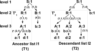
Figure 12: Two lists of nodes

Answering all-pairs reachability queries. To answer all-pairs reachability query, we traverse the two trees $T_{1}$ and $T_{2}$ representing $l_{1}$ and $l_{2}$ using Algorithm 2. This is done top-down, level by level. Note that children of the “same” node in $T_{1}$ and $T_{2}$ are either from the same simple workflow or from recursion (Cases 1 and 2, respectively, in Algorithm 2). For example, the children of $S:1$ in Fig. 12 are from the same simple workflow, whereas the children of $R:1$ are from recursion. Two nodes $v_{1},v_{2}$ in $T_{1},T_{2}$ are said to be same if they have the same labels, $\psi_{V}(v_{1})=\;\psi_{V}(v_{2})$. To disambiguate, we denote by $\psi_{T}(u)$ the label of the incoming edge of $u$ in $T$, e.g. $\psi_{T}(B:1)=(1,3)$.

Input: The tree presentations of two lists, $T_{1},T_{2}$, specification $G$ and safe query $R$

Initialization

Let $root(T)$, $children(T)$, $leaves(T)$ be the root of tree $T$, the set of children of the root, the set of leaf-descendants of the root; let $T(u)$ be the subtree rooted at node $u$

begin

   1 if $root(T_{1}),root(T_{2})$ are the same non-recursive node then

      // Case 1: Same simple workflow

       foreach $u\in children(T_{1}),v\in children(T_{2})$ do

          let $\psi_{T}(u)=(k,i),\psi_{T}(v)=(k,j)$

         2 if $i=j$ then $answerAllPairsSafeQuery(T(u),T(v))$

         3 else if The $i^{th}$ node reaches the $j^{th}$ node on the right-hand side of the $k^{th}$ production  then $output(leaves(T(u),leaves(T(v))))$

         

      

   4else if $root(T_{1}),root(T_{2})$ are the same recursive node then

       // Case 2: Recursion

       Let $Set_{op}$ ($op\in\{<,=,>\}$) be the set of all node pairs $(u,v)\in$ $children(T_{1})$ $\times children(T_{2})$ such that if let $\psi_{T}(u)=(s,t,i)$, $\psi_{T}(v)=(s,t,j)$ then $i~{}op~{}j$, and if $op$ equals $<$ then $u$ has red children, and if $op$ equals $>$ then $v$ has blue children

       // $Set_{op}$ can be computed by merge join; details are omitted

      5 foreach $(u,v)\in Set_{=}$ do

         $answerAllPairsSafeQuery(T(u),T(v))$

      6foreach $(u,v)\in Set_{<}$, red child $u_{r}$ of $u$ do

         $output(leaves(T(u_{r})),leaves(T(v)))$

      7foreach $(u,v)\in Set_{>}$, blue child $v_{b}$ of $v$ do

         $output(leaves(T(u)),leaves(T(v_{b})))$

      

   

output(a list of node labels $l_{1}$, a list of node labels $l_{2}$ ) {

 foreach  $u\in l_{1}$, $v\in l_{2}$ do 

8  if $\pi(\psi_{V}(u),\psi_{V}(v),G,R)$ then output($u$,$v$)}

Algorithm 2 answerAllPairsSafeQuery

For Case 1, let node $u$ of $T_{1}$ and node $v$ of $T_{2}$ be children of their respective root, and then $\psi_{T}(u)$ and $\psi_{T}(v)$ are of the form $(k,i)$. If $u$ can reach $v$ in the simple workflow for that production (line 3), then all leaf-descendant nodes of $u$ in $T_{1}$ can reach all leaf-descendant nodes of $v$ in $T_{2}$. However, if $u$ and $v$ are the same node, then we need to move to the next level to process the subtrees rooted at $u$ and $v$ (line 2). E.g., for $T_{1}$, $T_{2}$ in Fig. 12, we first process level 1. The outgoing edges of the root of $T_{1}$ are labeled $\{(1,2),(1,3)\}$, and $\{(1,2),(1,4)\}$ for $T_{2}$, and fall into case 1 (line 1). Note that $(1,2),(1,3),(1,4)$ corresponds to $A,B,b$ in $W_{1}$, respectively. It is clear that $A$ can reach $b$ and hence all leaf-descendants of $(1,2)$ in $T_{1}$ (i.e. $a:1,d:1$) are ancestors of all leaf-descendants of $(1,4)$ in $T_{2}$ ( i.e. $d:1$) (line 3). However, root of $T_{1}$ and $T_{2}$ have the same outgoing edge $(1,2)$. We then recursively process $T_{1}^{\prime}$ and $T_{2}^{\prime}$ (shown in the rectangles).

For Case 2, let a recursive node $u$ of $T_{1}$ and a recursive node $v$ of $T_{2}$ be a child of the root, and then $\psi_{T}(u)$ ($\psi_{T}(v)$) is of the form $(s,t,i)$ ($(s,t,j)$). Let $u_{r}$ be a child of $u$. If $u$ derives $v$, i.e. $i<j$ (line 6), and $u_{r}\leadsto v$ (i.e. $(u,u_{r})$ is a red edge) then leaf-descendants of $u_{r}$ can reach leaf-descendants of $v$. Similarly, if $v$ derives $u$, i.e. $i>j$ (line 7), and $u\leadsto v_{b}$ (i.e. $(v,v_{b})$ is a blue edge) then leaf-descendants of $u$ can reach leaf-descendants of $v_{b}$. If $u$ and $v$ are the same, we then move to the next level (line 5). E.g., $A:1~{}(1,1,1)$ of $T_{1}^{\prime}$ derives $A:2~{}(1,1,2)$ of $T_{2}^{\prime}$, hence all leaf-descendants of $a:1~{}(2,1)$ (red child) of $T_{1}^{\prime}$ can reach all leaf-descendants of $A:2$.

Answering all-pairs safe regular path queries. For each reachable node pair $(u,v)$ i.e. $u\leadsto v$, we invoke Algorithm 1 to check if $u\stackrel{{\scriptstyle R}}{{\leadsto}}v$ (Line 8).

Time complexity. Building the tree representation of a list can be done in time linear in the list size, assuming the list is sorted by post-order of nodes in the compressed parse tree. Case 1 does a nested-loop join. Since the size of the outer and inner loop of the join is bounded by the grammar size, this takes $O(|G|^{2})$. Case 2 does a merge join and hence takes $O(|l_{1}|+|l_{2}|)$. The body of the merge join runs in time linear in output size of the function $output$. For each level of the two trees, Algorithm 2 therefore takes $O(|l_{1}|+|l_{2}|+max(|l_{1}|,|l_{2}|)*|G|^{2}+N_{l})$ where $N_{l}$ is the number of reachable node pairs from this level. Since the height of the two trees is bounded by the grammar size, letting $l=\;max(|l_{1}|,|l_{2}|)$, Algorithm 2 takes $O(|G|^{3}l+N)$ where $N$ is the number of reachable node pairs in $l_{1},l_{2}$.

IV-B General queries

We now discuss answering general (unsafe) all-pairs regular path queries. We first describe three previous approaches, which will be used to provide a baseline for the experiments in the next section, and then describe our approach.

Option G1: Represent $R$ as a tree and evaluate bottom-up using joins [21]. This approach treats a regular expression as a (binary/unary) tree (parse tree), where leaves are single symbols, and internal nodes are union, concatenation, or Kleene star. We then evaluate the tree bottom-up. [24] is too slow we omit it.

Option G2: Use rare edge labels [20]. “Rare” edge labels are ones which match very few node pairs. The approach decomposes a query to a series of smaller subqueries using rare labels, then performs a breadth-first search on the graph.

Option G3: Use reachability labeling [3] combined with indexing for queries of a special form. Regular expressions of the form $R=(\_)^{*}a_{1}(\_)^{*}a_{2}(\_)^{*}\ldots(\_)^{*}a_{k}(\_)^{*}$ can be decomposed into $k$ sub-expressions of the form $R_{i}=a_{i}$. The set $l_{i}$ of nodes pairs $(u_{i},v_{i})$ matching $a_{i}$ can be found using indexing, and reachability tested between $v_{i}$ and $u_{i+1}$ using dynamic labeling.

Our approach: We first represent the regular expression $R$ as a (binary/unary) parse tree [21] as described in Option G1, and find its largest safe subtree, which then can be evaluated using the approach described in Section IV-A. The remainder of the query can then be evaluated using Option G1.

Given a tree representing $R$, to find the largest safe subtree, we traverse the tree top-down from the root. For each subtree, we check the safety of the regular expression it represents using the algorithm given in Section III-C. If the subtree is unsafe, we move to its child subtrees until we find a subtree that is safe. We will show in experiments that this simple heuristic yields significant performance improvements over previous approaches.

It is worth noting that there may be many trees equivalent to $R$ due to query rewriting [11]. Finding the largest safe subexpression is therefore an interesting optimization problem, which we leave for future work.

V Experiments

To evaluate the performance of all-pairs general regular path queries, we evaluate each component separately. We start in Section V-B by evaluating overhead, and then evaluate pairwise safe queries (Algorithm 1) in Section V-C and all-pairs safe queries (Algorithm 2) in Section V-D. Finally, we evaluate the performance of all-pairs general queries in Section V-E.

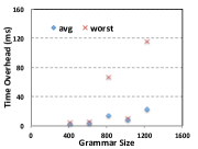
(a) Time overhead (vary grammar size)

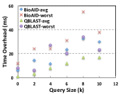
(b) Time overhead (vary query size)

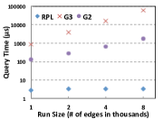
(c) pairwise query time (vary run size)

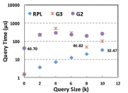
(d) pairwise query time (vary query size)

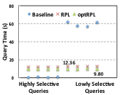
(e) all-pairs query time (BioAID)
$8$ IFQs ($k=3$), run size=$2K$

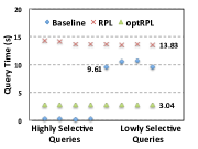
(f) all-pairs query time (QBLast)
$8$ IFQs ($k=3$), run size=$2K$

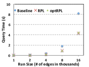
(g) all-pairs query time (BioAID)
$R=a^{*}$, run size=$2K$

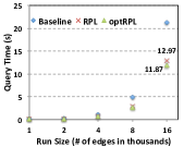
(h) all-pairs query time (QBLast)
$R=a^{*}$, run size=$2K$

Figure 13: Performance of our approaches (RPL and optRPL) for safe queries

V-A Experimental Setup

Experiments were performed on a Mac Pro with Intel Core i5 2.3GHz CPU and 4G memory. We use the library [1] to parse regular expressions and minimize DFAs. All reported running times are averages of 5 sample runs per setting.

Realistic and Synthetic Datasets. Realistic scientific workflows were collected from myExperiment [26]. We report on results for two representative, recursive workflows, BioAID and QBLast. BioAID is deep while QBLast is more “branchy”. BioAID, of size 166, has 112 modules (16 of which are composite) and 23 productions (7 of which are recursive); QBLast, of size 105, has 77 modules (11 of which are composite) and 15 productions (5 of which are recursive). To evaluate the overhead of our approach, we create a set of synthetic workflows while varying workflow parameters (e.g. size, recursion depth, node degree). Due to lack of space, we only report the overhead while varying workflow size.

Since myExperiment does not record executions, we simulate runs. If not specified, we apply a random sequence of productions, varying run sizes (i.e. the number of edges) from 1K to 8K by a factor of 2, and labeling the nodes as they are generated. All executions are stored as Java serializable objects on disk. The loading time is omitted.

In addition, we build indices to support comparisons (Option G3). For each run, an index maps an edge tag $\gamma\in\Gamma$ to a list of node pairs that are connected by an edge tagged $\gamma$. We store indices as Java serializable objects and materialize them on disk. The running time for all-pairs queries thus includes disk access for indices. Although we could further reduce the index access time by using more sophisticated indices, the inverted index is fast enough (below $10ms$) in light of the query time being more than $1s$.

Queries. We test using two classes of queries known to be expensive:

(1) IFQs ($R=(\_)^{*}a_{1}(\_)^{*}a_{2}\ldots a_{k}(\_)^{*}$) ask for node pairs that are processed by a sequence of modules. IFQs can be handled by indexing and reachability labels (Option G3), and are therefore challenging to improve upon. We will show that our approach beats the baseline when queries are not too selective.

(2) Kleene Star ($R=a^{*}$), used to query provenance for recursions, is at the other extreme. The baseline for Kleene star is Option G2, which performs self-joins on node pairs that are connected by an edge labeled $a$ until a fixpoint is reached. Since it is unknown how many rounds it takes to reach a fixpoint, the performance can be very bad. We will show that our approach achieves a major gain in this case.

It is worth noting that Kleene star is important for querying workflow provenance because of fork and loop operations. We illustrate by the simplest Kleene star expression $a^{*}$. For example, one fork operation in BioAID is captured by two productions shown in Fig. 14a, where module $A$ is composite, whose productions are omitted and module $M$ is to call $A$ in forks; atomic module $a$ is a fork distributor and atomic module $b$ is a fork aggregator. When executing, the first production may be fired many times, the result run of which is shown in Fig. 14b. When a user queries for data that are processed by forks, he may issue query $a^{*}$. To evaluate the performance of $a^{*}$, we generate runs by firing the specified fork recursion many times and other recursions only once, while varying run size from 1K to 16K by a factor of 2.

(a) Fork

(b) Run of Fork

Figure 14: A fork example of BioAID

We also generate queries by randomly combining edge tags using concatenation, union, and Kleene star. Due to space constraints, we do not explicitly list these queries.

V-B Overhead of Our Approach

In this section, we use RPL (Regular Path Labels) for our approach to pairwise queries (Algorithm 1) and Option S1 for all-pairs queries. We use optRPL for Option S2 (Algorithm 2).

The overhead of our approach comes from checking the safety of a query w.r.t. a workflow (Section III-C). We thus evaluate overhead while varying the grammar and query size. Fig. 13a shows the average and worst time overhead of $20$ IFQs with $k=3$ on synthetic workflows of size varying from $400$ to $1200$ ($10$ workflows per size). Fig. 13b shows the average and worst time overhead of IFQs varying $k$ from $0$ to $10$ on both BioAID and QBLast. We can see that time overhead increases as the grammar or query grows. Nonetheless the time overhead is $<200ms$, which is acceptable compared to the query time in seconds (see Section V-D).

V-C Performance of Pairwise Safe Queries

We test the performance of pairwise safe IFQs on real datasets while comparing Option G2 and G3 and RPL. Option G1 is clearly worse than Option G3 for IFQs so we omit it here. We vary run size and query size. QBLast has similar trends to BioAID, so we only report on BioAID. The pairwise query time is in microseconds, so we use $10K$ node pairs and report the average time of $5$ queries per setting. For RPL, the query time thus includes time overhead amortized over $10K$ node pairs. Fig. 13c reports the query time of IFQs of size $3$ on runs varying in size from $1K$ to $8K$. We can see that RPL runs in almost constant time (below $10\mu s$) while the run times of the other approaches grow sharply as the run size grows, from $100\mu s$ to $1ms$ and $1ms$ to $100ms$ respectively. Fig. 13d reports the query time of IFQs of size $k=0$ to $k=10$ on runs of size $2K$. We can see that the query time of RPL grows as the query size grows, but remains below $40\mu s$. In contrast, the query time of Option G2 and G3 goes above $40\mu s$. Note that when $k=0$, the query degrades to a reachability query and thus Option G3 has constant query time. It is worth noting that Option G2 and G3 do not show a clear trend; this is because they rely on query selectivity, which we will discuss in the next section. In summary, RPL significantly outperforms Options G2 and G3 for pairwise safe queries.

V-D Performance of All-pairs Safe Queries

We now show how labels can be used to help answer all-pairs safe queries. Since Option G2 is designed to run in parallel for all-pairs queries, it would be unfair to include it. So for IFQs, which favor existing approaches, the baseline is Option G3. For Kleene star, which favor our approach, the baseline is Option G1.

Fig. 13e reports the query time for $8$ IFQs of size 3 $k=3$ over runs of size $2K$ (the input lists $l_{1}$, $l_{2}$ are the list of all nodes) on BioAID. As expected, the baseline performance varies widely since it depends on the selectivity of the query. The first set of 4 queries are highly selective ( $<10$ node pairs), while the second set of 4 queries are not (around 100 node pairs). The baseline query time increases from $0.4s$ for the first set to $60s$ for the second set. In contrast, the performance of RPL and optRPL depend solely on the input list size (and query size), and have respective query times of $12s$ and $10s$ for all queries of this size, regardless of their selectivity. Compared with Fig. 13f, RPL is stable when query size and input list size are fixed while optRPL achieves a major gain over RPL. Note that query times of (opt)RPL for lowly selective queries on BioAID and QBLast vary, around 60s and 14s respectively; that is because BioAID is deeper so that IFQs match more node pairs.

Fig. 13g reports the query time for $a^{*}$ on BioAID. The query time of the baseline increases dramatically from $44ms$ to $7.8s$ as the run size grows from $1K$ to $16K$. In contrast, RPL and optRPL increase slowly from $22ms$ to $4.7s$, reducing the query time by an order of magnitude. The same trend can be observed in Fig. 13h for QBLast. Note that optRPL shows limited improvement over RPL because a relatively small number of unreachable node pairs are filtered out.

V-E Performance of General Queries

Finally, we evaluate the performance of regular path labels when used in general queries. We compare our approach optRPL with the baseline Option G1 on queries randomly generated by combining IFQs, Kleene stars and edge labels. We observed that most of the queries are safe. In this subsection, we only report the performance of $40$ unsafe queries. As expected, our technique significantly speeds up the performance of queries that generate massive intermediate results due to lowly selective components. For BioAID, 75% (31/40) of the unsafe queries were of this form; the improvement over the baseline of these queries is shown in Fig. 15a. Note that over 60% (19/31) of these queries show significant improvement ($>40\%$). For QBLast, over 25% (13/40) of the unsafe queries were of this form, and the improvement is shown in Fig. 15b. We therefore conclude that our technique could be a very useful component in a cost-based query optimizer that uses statistical information to choose the right query plan and would significantly reduce the evaluation cost of lowly selective subqueries.

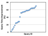
(a) BioAID

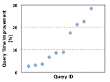
(b) QBLast

Figure 15: Improvement of optRPL for general queries

VI Conclusions

This paper considers the problem of answering regular path queries over workflow provenance graphs (executions). The approach assumes that the execution has been labeled with derivation-based reachability labels [4], and shows how to use them to answer regular path queries. For this we identify a core property of a query w.r.t. a specification, safe query, which allows reachability labels to be used in conjunction with the query-intersected specification to answer a pairwise regular path query in constant time. The reason that this works is that the reachability labels of [4], unlike other labeling techniques, are parameterized by the specification. Building on this, we develop efficient algorithms to answer all-pairs safe/general queries. Experimental results demonstrate the advantage of our approach, especially for queries which generate large intermediate results, e.g. Kleene star. Future work includes 1) building a cost model to predict the intermediate result size so as to optimize the query process; and 2) query rewriting, taking the workflow specification into account.

VII Acknowledgement

We thank the authors of [20] for providing their code.

References

- [1] http://www.brics.dk/automaton/.
- [2] S. Al-Khalifa et al. Structural joins: A primitive for efficient XML query pattern matching. In ICDE, 2002.
- [3] Z. Bao, S. B. Davidson, and T. Milo. Labeling recursive workflow executions on-the-fly. In SIGMOD, 2011.
- [4] Z. Bao, S. B. Davidson, and T. Milo. Labeling workflow views with fine-grained dependencies. In PVLDB, 2012.
- [5] Z. Bao et al. An optimal labeling scheme for workflow provenance using skeleton labels. In SIGMOD, 2010.
- [6] P. Barceló, L. Libkin, A. W. Lin, and P. T. Wood. Expressive languages for path queries over graph-structured data. ACM Trans. Database Syst., 37(4):31, 2012.
- [7] C. Beeri, A. Eyal, S. Kamenkovich, and T. Milo. Querying business processes. In VLDB, 2006.
- [8] A. Brüggemann-Klein and D. Wood. One-unambiguous regular languages. Inf. Comput., 140(2):229–253, 1998.
- [9] N. Bruno, N. Koudas, and D. Srivastava. Holistic twig joins: optimal XML pattern matching. In SIGMOD, 2002.
- [10] P. Buneman et al. Adding structure to unstructured data. In ICDT, 1997.
- [11] D. Calvanese et al. Rewriting of regular expressions and regular path queries. In PODS, pages 194–204, 1999.
- [12] L. Chen, A. Gupta, and M. E. Kurul. Stack-based algorithms for pattern matching on dags. In VLDB, 2005.
- [13] S. Cohen-Boulakia and U. Leser. Search, adapt, and reuse: the future of scientific workflows. SIGMOD Rec., (2):6–16, Sept. 2011.
- [14] S. B. Davidson et al. Provenance in scientific workflow systems. IEEE Data Eng. Bull., 30(4):44–50, 2007.
- [15] S. Dey, V. Cuevas-Vicenttín, S. Köhler, E. Gribkoff, M. Wang, and B. Ludäscher. On implementing provenance-aware regular path queries with relational query engines. EDBT, 2013.
- [16] M. F. Fernandez and D. Suciu. Optimizing regular path expressions using graph schemas. In ICDE, 1998.
- [17] T. Heinis and G. Alonso. Efficient lineage tracking for scientific workflows. In SIGMOD, pages 1007–1018, 2008.
- [18] J. Hopcroft, R. Motwani, and J. Ullman. Introduction to Automata Theory, Languages, And Computation. Pearson/Addison Wesley, 2007.
- [19] R. Jin et al. Computing label-constraint reachability in graph databases. In SIGMOD, 2010.
- [20] A. Koschmieder and U. Leser. Regular path queries on large graphs. In SSDBM, 2012.
- [21] Q. Li and B. Moon. Indexing and querying XML data for regular path expressions. In VLDB, 2001.
- [22] L. Libkin and D. Vrgoc. Regular path queries on graphs with data. In ICDT, 2012.
- [23] K. Losemann and W. Martens. The complexity of evaluating path expressions in SPARQL. In PODS, 2012.
- [24] A. O. Mendelzon and P. T. Wood. Finding regular simple paths in graph databases. In VLDB, 1989.
- [25] L. Moreau et al. The Open Provenance Model core specification (v1.1). Future Generation Computer Systems, (6):743 – 756, 2011.
- [26] D. D. Roure et al. The design and realisation of the myExperiment Virtual Research Environment for social sharing of workflows. Future Generation Comp. Syst., (5):561–567, 2009.
- [27] J. Starlinger, S. C. Boulakia, and U. Leser. (re)use in public scientific workflow repositories. In SSDBM, 2012.
- [28] S. Trißl and U. Leser. Fast and practical indexing and querying of very large graphs. In SIGMOD, 2007.
- [29] H. Wang et al. Coding-based join algorithms for structural queries on graph-structured XML documents. WWW, (4):485–510, 2008.
- [30] Q. Zeng and H. Zhuge. Comments on “Stack-based algorithms for pattern matching on dags”. PVLDB, (7):668–679, 2012.