Nonlinear Force-Free Field Modeling of the Solar Magnetic Carpet and Comparison with SDO/HMI and Sunrise/IMaX Observations

Abstract

In the quiet solar photosphere, the mixed polarity fields form a magnetic carpet, which continuously evolves due to dynamical interaction between the convective motions and magnetic field. This interplay is a viable source to heat the solar atmosphere. In this work, we used the line-of-sight (LOS) magnetograms obtained from the Helioseismic and Magnetic Imager (HMI) on the Solar Dynamics Observatory (SDO), and the Imaging Magnetograph eXperiment (IMaX) instrument on the Sunrise balloon-borne observatory, as time dependent lower boundary conditions, to study the evolution of the coronal magnetic field. We use a magneto-frictional relaxation method, including hyperdiffusion, to produce time series of three-dimensional (3D) nonlinear force-free fields from a sequence of photospheric LOS magnetograms. Vertical flows are added up to a height of 0.7 Mm in the modeling to simulate the non-force-freeness at the photosphere-chromosphere layers. Among the derived quantities, we study the spatial and temporal variations of the energy dissipation rate, and energy flux. Our results show that the energy deposited in the solar atmosphere is concentrated within 2 Mm of the photosphere and there is not sufficient energy flux at the base of the corona to cover radiative and conductive losses. Possible reasons and implications are discussed. Better observational constraints of the magnetic field in the chromosphere are crucial to understand the role of the magnetic carpet in coronal heating.

1. INTRODUCTION

The dynamical evolution of magnetic field in the solar photosphere holds the key to solving the problem of coronal heating. High resolution observations show that a mixed polarity field, termed as the magnetic carpet (Schrijver et al., 1997), is spread throughout the solar surface. The loops connecting these elements pierce through the atmosphere before closing down at the photosphere. The random motions of these small elements caused by relentless convective motions in the photosphere, are a favorite candidate to explain the energy balance in the solar atmosphere (for example, Schrijver et al., 1998; Gudiksen & Nordlund, 2002; Priest et al., 2002). In three-dimensional (3D) magnetohydrodynamic (MHD) models, small-scale footpoint motions drive dissipative Alfvén wave turbulence in coronal loops (van Ballegooijen et al., 2011). Also, the convective motions promote magnetic reconnection and flux cancellation—viable mechanisms to heat the corona (for example, Longcope & Kankelborg, 1999; Galsgaard & Parnell, 2005).

The magnetic carpet typically contains magnetic features with magnetic flux ranging from $10^{16}-10^{19}$ Mx, a part of which are kilo Gauss flux tubes, also in the internetwork (Lagg et al., 2010). The carpet is continually recycled with newly emerging flux replacing the pre-existing flux. Magnetic elements split, merge, and cancel due to granular action (Iida et al., 2012; Yang et al., 2012; Lamb et al., 2013). Additionally, recent observations show small-scale swirl events in the chromosphere, possibly due to the rotation of photospheric elements (Wedemeyer-Böhm & Rouppe van der Voort, 2009). Also, the magnetic elements display significant horizontal motions that can reach supersonic speeds (e.g. Jafarzadeh et al., 2013). All these dynamical aspects of the magnetic carpet make the overlying field non-potential—a source of magnetic energy (for a review on small-scale magnetic fields see de Wijn et al., 2009). There is indirect observational evidence for the existence of non-potential structures in the quiet Sun (Chesny et al., 2013).

The vector magnetic field ($\mathbf{B}$) or its line-of-sight component ($B_{z}$) at the photosphere is used to infer coronal fields, due to the unavailability of their direct measurements in corona. Earlier studies of the co-evolution of magnetic carpet and coronal field were mainly through the potential field (current-free) extrapolations of the photospheric magnetic field (for example, Close et al., 2004; Schrijver & van Ballegooijen, 2005). Recently,  Meyer et al. (2013) have used nonlinear force-free field extrapolations of the observed $B_{z}$ to study the magnetic energy storage and dissipation in the quiet Sun corona. They concluded that the magnetic free energy stored in the coronal field is sufficient to explain structures like X-ray bright points (XBP) and other impulsive events at small-scales  (for reviews on the force-free magnetic fields see Schrijver et al., 2006; Metcalf et al., 2008; Wiegelmann & Sakurai, 2012). Wiegelmann et al. (2013) have used a 22 minute time sequence of very high resolution vector magnetograms to extrapolate the field into the upper atmosphere under the potential field assumption, and argued that the energy release through magnetic-reconnection is not likely to be the primary contributor to the heating of solar chromosphere and corona in the quiet Sun. To test the basis of magnetic-reconnection between open and closed flux tubes as a plasma injection mechanism into the solar wind, Cranmer & van Ballegooijen (2010) used Monte Carlo simulations of the magnetic carpet. They also concluded that the slow or fast solar wind is unlikely to be driven by loop-opening processes through reconnections. The works of Cranmer & van Ballegooijen (2010) (using models to study solar wind acceleration), and Wiegelmann et al. (2013) (using observations to study solar atmospheric heating) arrive at similar conclusions, disfavoring a significant role of the evolution of the magnetic carpet in supplying energy to the corona and solar wind, in contrast to Meyer et al. (2013).

A possible explanation for the above conflicting results is that the potential field studies simplify the magnetic topology and do not include dynamic aspects like currents, and other nonlinear effects. Also, as the methods of analysis are not the same, it may not be so straightforward to compare the results from those studies. With an ever increasing quality of the observations showing more intermittent flux filling the solar surface, it is valid to inquire its contribution to the dynamics of the upper solar atmosphere and advance our knowledge towards a holistic picture of the magnetic connection from photosphere to corona, particularly in the quiet Sun.

To rigorously address these issues, a continuous monitoring of the Sun’s magnetic field is desired. This valuable facility is provided by the Helioseismic and Magnetic Imager (HMI; Scherrer et al., 2012) on board the Solar Dynamics Observatory (SDO; Pesnell et al., 2012). SDO/HMI obtains full-disk magnetograms of the Sun at $0^{\prime\prime}.5$ pixel^-1 with 45 s cadence. To probe the magnetic field at an even higher spatial resolution, the Imaging Magnetograph eXperiment (IMaX; Martínez Pillet et al., 2011) instrument on the Sunrise balloon-borne observatory (Solanki et al., 2010; Barthol et al., 2011) recorded 33 s cadence observations at $0^{\prime\prime}.055$ pixel^-1. To better understand the role of the magnetic carpet, we use the SDO/HMI and the Sunrise/IMaX line-of-sight (LOS) magnetic field observations as lower boundary conditions in a time-dependent nonlinear force-free modeling of the coronal field, and report our comparative findings. The rest of the paper is structured as follows. In Section 2 we describe the datasets, and model set-up. In Section 3 the main results of the work are presented. We conclude in Section 4 with a summary, and implications of the results are discussed.

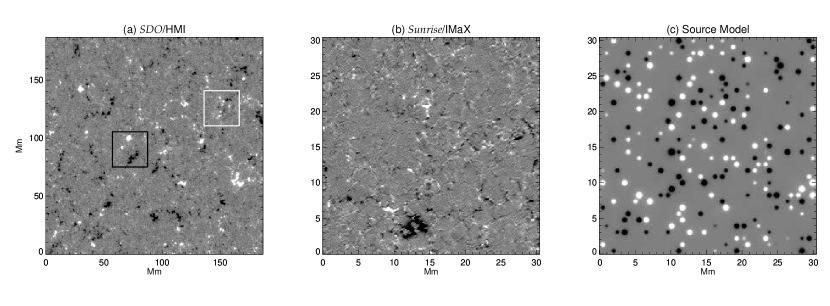
Figure 1.— Contextual figure showing the photospheric line-of-sight (LOS) magnetograms taken from the respective time sequences. (a) SDO/HMI. (b) Sunrise/IMaX. (c) Model magnetogram from the magnetic sources (see text for details). Note the larger field of view (FOV) of SDO/HMI compared to the Sunrise/IMaX, and Source Model. A white box shown in panel (a) is approximately the size of FOVs in panels (b), and (c). To facilitate displaying, all the magnetograms are saturated at $\pm 50$ G.

2. OBSERVATIONS AND MODEL SET-UP

In this work we used a one day long time sequence of the SDO/HMI LOS magnetic field observations at the disk center and compared the results with the higher resolution observations at the disk center obtained from the Sunrise/IMaX instrument. In Section 2.1 we briefly describe the datasets, and Section 2.2 deals with the set-up of the simulation for the magnetic field extrapolations.

2.1. Dataset

HMI Data (Set 1): This set consists of a tracked, one day long, time sequence of the LOS magnetograms observed at the disk center on 2011 January 08, starting at 00:00 UT. With a field-of-view (FOV) of $187\times 187$ Mm², and a time cadence of 45 s, these observations cover several magnetic network patches in the quiet Sun. In Figure 1(a) we show a snapshot from the HMI observations. The magnetic flux density is saturated at 50 G. The observations are found to be closely in flux balance over the entire duration. To retain the weaker field at the lower boundary, no smoothing is applied to the data. The larger region considered here allows us to compare various results between sub-regions with varied magnetic configurations. The details are given in Section 3.

Figure 2.— Mean magnetic field as a function of time for the three magnetogram types. (a) SDO/HMI (solid line, the mean magnetic field is derived from a region marked with the white box in Figure 1(a)), Source Model (dashed line). (b) Sunrise/IMaX. The $y$-axis scaling for both panels is the same.

IMaX Data (Set 2): These level 2 data correspond to imaging spectropolarimetric observations of Fe i at 5250.2 Å. The observations were recorded at the disk center on 2009 June 09, starting at 01:30 UT. The spatial resolution of these observations is ten times better than the HMI sequence. On the downside, IMaX observations span over time period of only $\approx 30$ minutes. From the original frames, the degraded edges because of the apodization (required by the phase diversity restoration technique) during the reduction process have been discarded. We extracted a $30\times 30$ Mm² region for further analysis. The LOS magnetograms are derived by taking the ratio of Stokes $V$ and $I$ with a calibration constant  (cf. Eq. 17, Martínez Pillet et al., 2011). The data are binned to a pixel scale of 119.2 km (Figure 1(b)). This effectively reduces the noise in the data by up to a factor of three (but it also reduces signal due to small-scale mixed polarity fields). Similar to the HMI data, IMaX data are also found to be closely in flux balance. Due to the limitations of the time duration of the dataset, the evolution of the coronal magnetic field cannot be studied for a longer period. For this purpose, we have constructed a series of artificial LOS magnetograms, named, Source Model. The details of the Source Model are given below.

Source Model (Set 3): The Source Model is made to complement the IMaX observations, but for a longer duration of time (see Appendix A for details). The model is initiated with $50$ magnetic sources placed randomly on a mesh of hexagonal grids (which has the dimensions of IMaX FOV considered above). The mesh is periodic in $x$-, and $y$-directions. The sources include both positive and negative polarity elements such that the net flux is zero. The sources are allowed to move along the edges of each hexagonal grid which has a length unit of $\approx 1$ Mm. All the sources move with a uniform velocity of 1.5 km s^-1, which is in the range of typical observed velocities of the small scale magnetic elements due to the interactions with granules (for e.g. Chitta et al., 2012, and references therein).

During the time evolution, the flux emergence, cancellation, along with splitting and merging of the elements are the possible ways of interactions among the magnetic elements at the corners of each grid. The LOS magnetic field reached a quasi-statistical equilibrium almost 15 hours after the initiation. During this time, the total magnetic flux increased from $10^{19}$ Mx to $10^{20}$ Mx. Out of the total 48 hours of time evolution, which includes both the rise time and equilibrium period, a portion of 8.5 hours time sequence is used for further analysis. The total flux in the Source Model FOV roughly matches with that of the IMaX observations. In Figure 1(c) we show a snapshot of the LOS magnetogram from the Source Model.

To ensure $\nabla{\cdot}\mathbf{B}=0$, fractional flux imbalance in the observed data (HMI and IMaX) is corrected by dividing the positive flux with an absolute ratio of integrated positive flux to the negative flux in the FOV. This method is justified only if the ratio is close to unity to begin with, in other words, the observations must be closely in flux balance. This is the case in both the observations we used in this study. In Figure 2 we plot the mean magnetic field ($\langle|B_{z}|\rangle$) as a function of time for all the datasets. In the left panel the solid line is for the HMI set and dashed line is for the Source Model. Right panel shows the IMaX mean magnetic field. We emphasize that the IMaX LOS magnetic field is derived from a simple ratio method, which underestimates the flux density in stronger elements (Martínez Pillet et al., 2011).

Table 1Values of $L$, $T$, $\eta_{4}$ and $\nu^{-1}$ used in the magnetic modeling

	$L$ (Mm)	$T$ (s)	$\eta_{4}$ (km4 s-1)	$\nu^{-1}$ (km2 s-1)
HMI	3.12	900	$1.05\times 10^{7}$	$1\times 10^{3}$
IMaX	1.02	165	$6.48\times 10^{6}$	$0.6\times 10^{3}$
Source Model	1.02	680	$1.57\times 10^{6}$	$0.1\times 10^{3}$

2.2. Simulation Set-up

In this section we describe the simulation set-up and the equations we solve to derive the 3D magnetic field above the photosphere.

For Set 1, the computational box is a $512\times 512\times 250$ cell volume covering $187\times 187\times 91.4$ Mm³ in physical space. For Sets 2 and 3, the computational domain is much smaller covering only $30.5\times 30.5\times 18$ Mm³ with $256\times 256\times 150$ cells. The simulation box is periodic in $x$- and $y$-directions and closed at the top. LOS magnetograms of Sets 1, 2, and 3 are the respective boundary conditions in the $xy$-plane at $z=0$. Initially, at time $t=0$, a potential field is assumed to fill the box, which is then evolved in time into nonlinear force-free states with the evolving boundary conditions.

The rate of change of vector potential $\mathbf{A}$ is related to the magnetic field $\mathbf{B}$ through the induction equation

$$\frac{\partial\mathbf{A}}{\partial t}=\mathbf{v}\times\mathbf{B}+\epsilon,$$ (1)

where $\epsilon$ is the hyperdiffusion, defined as

$$\epsilon=\frac{\mathbf{B}}{B^{2}}\nabla\mathbf{\cdot}(\eta_{4}B^{2}\nabla\alpha).$$ (2)

$\alpha={\mathbf{j{\cdot}B}}/{B^{2}}$ is the force-free parameter, and $\eta_{4}$ is the hyperdiffusivity. Some form of magnetic diffusion is needed in any numerical MHD simulation to suppress the development of numerical artifacts on small spatial scales. Here we use hyperdiffusion (instead of ordinary resistivity) to minimize the direct effect of the diffusion on larger scales. van Ballegooijen & Cranmer (2008) presented a theory of coronal heating which draws energy with hyperdiffusion from the dissipation of nonpotential magnetic field. It conserves the mean magnetic helicity and smooths the gradients in $\alpha$ (Boozer, 1986; Bhattacharjee & Hameiri, 1986). It has been proposed that tearing modes can promote turbulence in 3D sheared magnetic field, which causes hyperdiffusion (Strauss, 1988).

Equation 1 is evolved using a magneto-frictional relaxation technique (Yang et al., 1986), which assumes that the plasma velocity ($\mathbf{v}$, in this case, the magneto-frictional velocity) is proportional to the Lorentz force ($\mathbf{j}\times\mathbf{B}$), given by

$$\mathbf{v}=\frac{1}{\nu}\frac{\mathbf{j}\times\mathbf{B}}{B^{2}},$$ (3)

where $\nu$ is the frictional coefficient. The numerical values of $\eta_{4}$ and $\nu^{-1}$ (tabulated in Table 1) are determined in part by the requirement of numerical stability of the code, and by the length ($L$) and time ($T$) units of the simulations. Mackay et al. (2011) and Cheung & DeRosa (2012) used magneto-frictional relaxation technique to study the time evolution of active regions on much larger scales.

It is known that the magnetic field in the photosphere is non-force-free due to the high plasma $\beta$. Metcalf et al. (1995) calculated the Lorentz force of an active region as a function of height. They concluded that the field becomes force-free higher in the atmosphere, above approximately 400 km. The mixed polarity fields in the magnetic carpet are weaker and may be dominated by gas pressure even in the chromosphere as suggested by the simulations of Abbett (2007), which, however, do not include a realistic treatment of radiative transfer for the photospheric and chromospheric layers. To mimic the additional forces on the magnetic field in the photosphere and low chromosphere, we use the method first described by Metcalf et al. (2008) where a second term is added to the magnetofrictional velocity

$$\mathbf{v}=(\frac{1}{\nu}\mathbf{j}-v_{1}\hat{z}\times\mathbf{B})\times\mathbf{B}/B^{2}.$$ (4)

The additional term is present only at low heights (up to 0.7 Mm) and is the projection of a constant upward velocity ($v_{1}\hat{z}$) onto the plane perpendicular to the local magnetic field. The quantity $v_{1}$ is constant over horizontal planes and independent of the magnetic field. This new force marginally prevents the field from splaying out at the lower boundary. In the present paper we use $v_{1}=1.5$ km s^-1 for IMaX/Source Model, and $v_{1}=3.4$ km s^-1 for HMI dataset. This has only a minor effect on the flux concentrations in our model. Similar to $\eta_{4}$ and $\nu^{-1}$, the choice of $v_{1}$ is defined by the $L$ and $T$ units of the respective models.

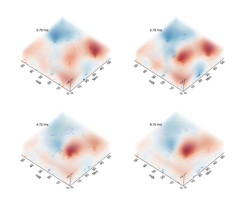
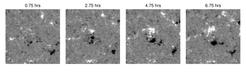
Figure 3.— Top segment: Volume rendering of the extrapolated $B_{z}$ using SDO/HMI observations as lower boundary conditions. Shown here is the time evolution of $B_{z}$ of an ephemeral region, with consecutive frames lying two hours apart, in a box of $\approx 55\times 55\times 14$ Mm³ volume, with its bottom surface centered at (70 Mm, 90 Mm) of Figure 1(a). The red (blue) colored areas are the regions of negative (positive) polarity. Bottom segment: The distribution of $B_{z}$ (saturated at $\pm 50$ G) in the photosphere corresponding to the respective panels in the top segment is shown.

3. RESULTS

In the top segment of Figure 3 we present volume rendering of $B_{z}$ in a sub-volume from HMI simulations, at four instances, separated by two hours each. At the lower boundary of this sub-volume an emerging bipole is seen, with stronger negative polarity (centered on the black square, Figure 1(a)). The red (blue) coloration covers regions of negative (positive) polarity. As the bipole emerges into the atmosphere, pre-existing coronal field responds to it, and eventually becomes bipolar in time. Note that this is a 3D rendering. To see through the cube, we used increasing transparency of layers with height (so that we can see till the bottom through the layers above). Also, to account for the decrease in field strength with height, we scaled each layer (at a given height) in respective panels separately. In the bottom segment we show $B_{z}$ at photospheric level corresponding to the respective panels in the top segment. The purpose of this figure is to show how the coronal field responds to an emerging bipole in the photosphere.

Figure 4.— Top panel: Free energy of an emerging bipole located within the black square in Figure 1(a). Each of the four curves plotted in a different line style is for a different point in time, corresponding to the times of the snapshots plotted in Figure 3. The curves are labelled in the upper panel. At all times $E_{\text{free}}(z)$ falls rapidly with $z$, peaking below 5 Mm. Bottom panel: The ratio of non-potential magnetic energy to the potential magnetic energy ($\gamma$) is plotted as a function of height (for the same time steps as shown in the top panel). The peaks of $\gamma(z)$ shift towards higher $z$ with time, indicating the interaction of newly emerging field with the pre-existing coronal field.

The magnetic free energy ($E_{\text{free}}$), which is an excess of non-potential magnetic energy (in this case, the nonlinear force-free energy) over the potential magnetic energy is calculated. Our aim is to emphasize the height dependence of the quantities relevant to the energy budget of the solar corona. To this end, we calculate $E_{\text{free}}$ as a function of height, given by

$$E_{\text{free}}(z)=\frac{1}{8\pi}\Delta z\int\int[B^{2}_{\text{np}}(x,y,z)-B^{2}_{\text{p}}(x,y,z)]dxdy,$$ (5)

where $\Delta z$ is the pixel length. $B^{2}_{\text{np}}/8\pi$ and $B^{2}_{\text{p}}/8\pi$ are the non-potential, and potential magnetic energy densities, respectively. In the top panel of Figure 4 we plot the HMI $E_{\text{free}}(z)$ ($\Delta z=0.36$ Mm). Integration is over the surface enclosed by the black square in Figure 1(a). The curves represent the evolution of an emerging bipole at four times (shown in Figure 3). It is observed that most of $E_{\text{free}}(z)$ (5–10$\times 10^{25}$ ergs), is available at heights below 5 Mm. These results are consistent with the free energy values reported in Meyer et al. (2013).

To estimate the non-potentiality of the magnetic energy, we calculate a ratio $\gamma(z)$, defined as

$$\gamma(z)=\frac{\int\int B^{2}_{\text{np}}(x,y,z)dxdy}{\int\int B^{2}_{\text{p}}(x,y,z)dxdy}.$$ (6)

It is observed that the magnetic energy is close to energy of the potential magnetic field, with an excess $<20$%. In the bottom panel of Figure 4 we plot $\gamma(z)$ for the same time steps as shown in the top panel. There is an apparent rise in the non-potentiality with time, indicating the interaction of a newly emerging flux with the pre-existing coronal field. However, by combining the values of $\gamma(z)$ and $E_{\text{free}}(z)$, it can be seen that the coronal field over the HMI FOV is potential. We note that in the bottom panel, $\gamma(z)<1$ for some points in time above a height of $10$ Mm, which means a negative free energy. This is due to the fact that the surface integration is performed only over a sub-region within the full FOV. The total volume integrated $E_{\text{free}}$, however, remains positive.

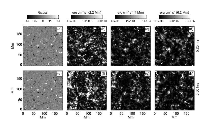
Figure 5.— HMI Magnetic field configuration at the lower boundary ((a) and (e) saturated at $\pm 50$ G), and the energy dissipation ($Q$) at three layers ((b) and (f) 2.2 Mm; (c) and (g) 4 Mm; (d) and (h) 6.2 Mm) are shown. Note the change of grey scale ranges in the energy dissipation maps. The top and the bottom maps are separated by 15 minutes in time and are rendered according to the same greyscales (for a given height). Though the magnetic field configuration has little apparent change, the locations of the energy dissipation have changed significantly, suggesting a highly non-localized and intermittent nature of the time evolution of magneto-frictional relaxation method.

Magnetic free energy is necessary but not sufficient to completely quantify the energy supply to solar corona. It is important to calculate the energy dissipation, and energy flux, which can then be directly compared with the observed radiative and conductive losses. Earlier studies by Withbroe & Noyes (1977), Withbroe (1988), Habbal & Grace (1991) placed observational constraints on the energy flux through the coronal base, $10^{5}$–$10^{6}$ erg cm^-2 s^-1 for a quiet Sun region. With magneto-frictional relaxation including hyperdiffusion, the energy dissipation per unit volume ($Q$) is calculated as

$$Q=\frac{B^{2}}{4\pi}(\nu|\mathbf{v}|^{2}+\eta_{4}|\nabla\alpha|^{2}),$$ (7)

(see, Yang et al., 1986; van Ballegooijen & Cranmer, 2008). The first and second parts on the right hand side of the Equation 7 are due to magneto-friction, and hyperdiffusion, respectively. To understand the evolution of $Q$ with respect to height, at the time scale of minutes, we consider snapshots of $Q$ from HMI simulations, separated by 15 minutes. The results are shown in Figure 5. The top row shows $B_{z}$ (lower boundary, (a)), and $Q$ at three heights ((b): 2.2 Mm, (c): 4 Mm, and (d): 6.2 Mm) at 5.25 hrs into the simulation. Bottom row is same as the top row, but 15 minutes after panels (a)-(d). With very little change in the $B_{z}$ over the duration, apparently, there is a drastic morphological change in $Q$ (panels (b) and (f)). This is very interesting to note, suggesting that the energy dissipation process due to magneto-friction and hyperdiffusion is non-localized in time (i.e., the locations of energy dissipation rapidly change with time). This in turn means that the time evolution of spatially averaged $Q$ at any two locations separated by some distance (having a different underlying magnetic morphology) would be similar. In other words, the average dissipation of magnetic energy is very uniform in our simulations. However, the magnitude of $Q$ has a strong height dependence (as seen in the greyscales of the right three panels). This was also indicated by Meyer et al. (2013). These large-scale changes in the atmosphere are caused by small-scale random footpoint motions of magnetic elements at the photosphere.

Figure 6.— Horizontal mean of energy dissipation plotted as a function of height (top panels), and time (bottom panels). (a) Mean energy dissipation over an ER (red), and a QR (blue) observed by HMI. (b) Energy dissipation in the IMaX dataset (blue) and Source Model (red) averaged over the entire FOV. As an illustration, a grey striped box is drawn at 2–6 Mm range to compare the energy dissipations between panels (a), and (b) at those heights. (c) Mean energy dissipation plotted vs. time, averaged over the height ranges 0–2 Mm (solid) and 2–4 Mm (dashed), respectively. (d) Same as (c), but for Source Model.

To further quantify the above statements, Figure 6 plots the horizontally averaged dissipation rate as a function of height and time. The top left panel is $Q$ plotted as a function of height from the HMI simulations. The two shaded bands are for two sub-regions of the HMI FOV (red: Figure 1(a) black square; blue Figure 1(a) white square). The black square covers an ephemeral region (ER), and the white square covers a less active quiet region (QR). At a given height, the width of each shaded band represent the range of minimum to maximum energy dissipated at that height. A vertical shaded rectangle is drawn to indicate the base of the transition region and corona. $Q$ monotonically decreases with height in a similar way for regions with completely different underlying $B_{z}$. In the top right panel, results from the Source Model (red), and IMaX (blue) are shown for comparison with those of HMI. It is noted that the fall of $Q_{\text{Source Model/IMaX}}$ is steeper than $Q_{\text{HMI}}$.

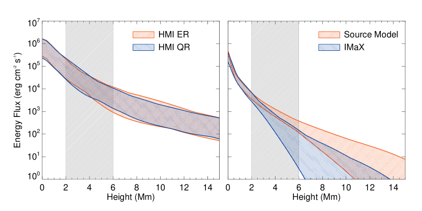
Figure 7.— Horizontal mean of the energy flux plotted as function of height. The color schemes and legends in the left and right panels are the same as in Figures 6(a) and (b), respectively.

Further, we plot the averaged $Q$ in two height ranges (0–2; 2–4 Mm) and study its time evolution. In Figure 6(c) we plot these results for the HMI simulations (red: ER; blue: QR; solid: 0–2 Mm; dashed: 2–4 Mm). These plots show that on average, the energy dissipation is uniform over the entire FOV and also fairly constant throughout the time evolution. Another fact to notice is that $Q$ reaches its statistically mean value very early in the simulations. Recalling that the initial condition of the simulation is a potential field, the build-up of magnetic shear of coronal field and in turn the energy dissipation through hyperdiffusion, is contributing only a fraction of total $Q$. Magneto-friction acts as a dominant energy source in our simulations. Figure 6(d) shows the evolution of $Q_{\text{Source Model}}$.

As a next step, we calculate the energy flux ($F$) through a given horizontal surface. In a quasi-stationary state, the energy flux $F(z)$ through height $z$ is equal to the integral of $Q(z)$ over all heights above $z$, given by

$$F(z)=\int_{z}^{z_{max}}Q(z)dz,$$ (8)

where $z_{max}$ is the top of the simulation domain. The horizontal average of the calculated $F(z)$ is plotted in Figure 7. Similar to Figure 6(a), in the left panel we show $\langle F(z)\rangle$ for two sub-regions within HMI FOV. $\langle F(z)\rangle$ of IMaX/Source Model are plotted in the right panel. All sets have a flux of $\approx 10^{6}$ erg cm^-2 s^-1 at the photosphere. Almost all of this flux is dissipated at heights below 2 Mm, i.e. in the chromosphere (for which, however, our model may not be valid, since the field below 1000–1500 km is not force-free). Over a quiet Sun, the coronal base is typically above 3 Mm (cf. Figure 3, Withbroe & Noyes, 1977). At this layer, $\langle F_{\text{HMI}}(z)\rangle\approx 5\times 10^{4}$ erg cm^-2 s^-1, and $\langle F_{\text{IMaX}}(z)\rangle\approx 2\times 10^{3}$ erg cm^-2 s^-1. These values are lower than the required flux in the quiet Sun corona.

To summarize Figures 6 and 7, three sets of magnetograms used in this work show a similar trend. Close to the lower boundary both $Q(z)$, and $F(z)$, respectively, are similar for all the cases. $F(z)$ is $>10^{5}$ erg cm^-2 s^-1, and appears to be comparable with the coronal energy budget of the quiet Sun. This condition is no more satisfied for $z>$2–3 Mm. On average, there is an order of magnitude or more deficit in the required energy flux to support the observed coronal energy losses. The deficit in $F(z)$ is very noticeable in the higher resolution but smaller FOV IMaX/Source Model cases.

Figure 8.— The dependence of energy flux on the dimensionless parameters ($\theta$, $\phi$) is shown for the case of IMaX dataset. The ratio $F^{\prime}_{\theta,\phi}(z)/F(z)$ is plotted as a function of height for three sets of parameters as marked in the plot legend (see text for details).

Next, choosing IMaX set as an example we studied the dependence and sensitivity of the calculated energy dissipation and flux on the simulation parameters ($\nu^{-1}$, $\eta_{4}$). As described in the previous section, the numerical values of these parameters are constrained by the requirements that the code be numerically stable and that numerical artifacts are suppressed. The frictional coefficient and hyperdiffusivity can be written as $\nu^{-1}=\theta L^{2}/T$ and $\eta_{4}=\phi L^{4}/T$, where $\theta$ and $\phi$ are dimensionless parameters, and $L$ and $T$ are the length and time units for each simulation. For the case of IMaX (and also for the Source Model), $\theta=0.1$ and $\phi=0.001$; the corresponding values of $\nu^{-1}$ and $\eta_{4}$ are listed in Table 1. Numerical stability dictates that $\theta$ and $\phi$ cannot be arbitrarily large, and to suppress numerical artifacts $\phi$ cannot be arbitrarily small. To test how lower values of these parameters affect the final results, we considered three sub-cases: (a) $\theta=0.01$, $\phi=0.0001$; (b) $\theta=0.01$, $\phi=0.001$; (c) $\theta=0.1$, $\phi=0.0001$. Further, the energy flux with the respective new set of parameters is calculated, and we denote it as $F^{\prime}_{\theta,\phi}(z)$. The ratio $F^{\prime}_{\theta,\phi}(z)/F(z)$ is plotted in Figure 8 (solid line: case (a); dashed line: case (b); dash-dotted line: case(c)). Here, $F(z)$ is calculated with $\theta=0.1$ and $\phi=0.001$ (see the blue shaded band in the right panel of Figure 7). These results indicate that the energy dissipation and flux are sensitive to the frictional coefficient, which can also be argued on the basis that the magneto-frictional energy is dominant in the simulations.

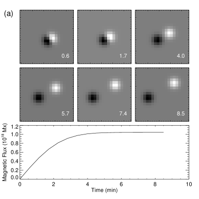
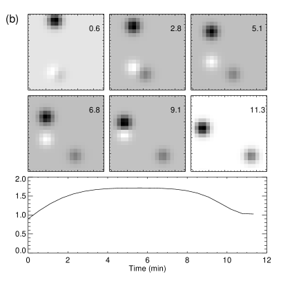
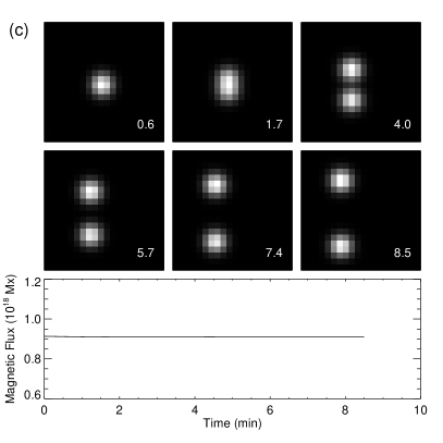
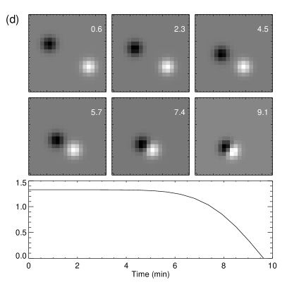
Figure 9.— Various interactions among magnetic elements in the Source Model are illustrated here. (a) Flux emergence. (b) Flux emergence followed by a partial flux cancellation. (c) Flux splitting. (d) Total flux cancellation. Each panel is comprised of two segments. The top segment is a time sequence of magnetic maps describing the interaction. Each map in the respective top segment covers an area of $\approx 2.4\times 2.4$ Mm². The numbers in the maps indicate time, in minutes, elapsed since an arbitrary start time. The bottom segment is a plot of the magnetic flux integrated over the area of the map as a function of time. The scale of $y$-axis in the bottom segment is set at 10¹⁸ Mx.

4. SUMMARY AND DISCUSSION

With an aim to understand the role of the magnetic carpet in the heating of the solar corona, we simulated the coronal magnetic field using the disk center observations of quiet Sun LOS magnetic field obtained from the SDO/HMI and Sunrise/IMaX. To overcome the limitations of short duration IMaX data, we created a time sequence of synthetic magnetograms that roughly match the IMaX set in terms of the absolute flux (Figures 1–2). A time series of the 3D nonlinear force-free magnetic field is constructed with the magnetograms as lower boundary conditions, and potential fields as initial conditions. The coronal field is evolved using Equation 1, with a magneto-frictional relaxation technique (Equation 4), including hyperdiffusion (Equation 2). We incorporated the non-force-free nature of the lower solar atmosphere ($\leq 0.7$ Mm) by adding vertical flows that prevent the field from splaying out at the lower boundary (Equation 4). These gentle flows weakly increased the field strength of the magnetic elements.

Next, we calculated $E_{\text{free}}(z)$, $Q(z)$, and $F(z)$ to quantitatively estimate the magnetic free energy, its dissipation, and energy flux injected at the base of corona. It is found that the energy dissipation in simulations with moderate resolution (HMI), and much higher resolution (IMaX/Source Model), is very similar close to the lower boundary. At low heights in these models most of the heating occurs in short, low-lying loops that originate from the mixed-polarity magnetic carpet. The average length of these loops is only a small fraction of the computational domain. Further, these loops are highly intermittent, facilitating uniform energy dissipation over the entire surface. These loops can be formed by interactions of near-by elements (e.g. Wiegelmann et al., 2010), and also from the newly emerging flux in the internetwork (Centeno et al., 2007).

Despite their intrinsic differences, IMaX and Source Model simulations are strikingly similar. Moving away from the lower boundary, we see that $F_{\text{Source Model/IMaX}}$ decreases by more than two orders of magnitude at $z=2$ Mm. This leaves only a few percent of $F$ at the coronal base. The energy flux into the corona as predicted by our model is approximately $10^{4}$ $\rm erg~{}cm^{-2}~{}s^{-1}$ (see the right panel of Figure 7), which is about one order of magnitude smaller than the estimated radiative and conductive losses from the quiet-Sun corona as derived from EUV and X-ray observations (e.g., Withbroe & Noyes, 1977; Withbroe, 1988; Habbal & Grace, 1991). We conclude that the present model, which is based on evolving force-free magnetic fields and uses realistic photospheric boundary conditions, cannot account for the observed coronal heating of the quiet Sun.

Figure 10.— The complete time evolution of the magnetic flux for the Source Model, integrated over its FOV is shown. The plot includes both the rise and equilibrium phases of the magnetic flux as described in Section 2.1. Two thin vertical lines mark the period of 8.5 hours duration from which the time sequence of the Source Model is extracted for further analysis.

Wiegelmann et al. (2013) used similar IMaX data to create a set of potential field models of the evolving magnetic carpet. They also concluded that the magnetic energy release associated with reconnections is not likely to supply the required energy to heat the chromosphere and corona. Our estimate for the energy flux $F$ into the corona is below the upper limit provided by Wiegelmann et al. (2013), indicating that flux estimates based on force-free-field modeling are consistent with those based on potential field modeling. However, both types of estimates are well below the values needed to heat the corona. This suggests that both potential-field and force-free-field models underestimate the amount of energy injected into the corona due to photospheric footpoint motions and other effects in the magnetic carpet. This is perhaps not surprising because these models make many simplifying assumptions about the structure and dynamics of the solar atmosphere. For example, the models ignore the details of the lower atmosphere, where the density decreases with height over many orders of magnitude. Also, the models assume that the coronal magnetic field evolves quasi-statically in response to the footpoint motions, whereas in reality the response may be more dynamic and significantly more energy may be injected in the form of Alfvén waves (e.g., van Ballegooijen et al., 2014).

However, the deficit in $F$ is smaller in the HMI set as compared to those of other models. Assuming that this discrepancy is mainly due to the larger HMI volume, it means that there is a contribution from the long range magnetic connections, often reaching coronal heights, that was not possible with the IMaX set. This was also cited by Wiegelmann et al. (2013) as a reason for their too low upper limit. Future observations with high spatial resolution and large FOVs are required to check and justify the contribution from long range magnetic interactions. Also, IMaX and HMI observed mainly different kinds of features, with very different lifetimes. In the case of HMI it is predominantly network magnetic features (including ephemeral regions) and some internetwork fields, for IMaX it is dominated by internetwork fields. The latter are more likely to be horizontal and do not reach high into the atmosphere. Additionally, IMaX observations were carried out in 2009, at the depth of the last minimum in a very quiet part of the Sun, while the HMI data were obtained in 2011, i.e. when the Sun was well on its way into the new cycle.

A relatively large $F_{\text{HMI}}(z)$ can be considered as a basal flux to heat a diffused coronal region. Compact features like XBPs have a mean lifetime of eight hours (Golub et al., 1974), and an average emission height of 8–12 Mm above the photosphere (Brajša et al., 2004; Tian et al., 2007). Our model predicts a flux too small to account for the energy losses at those height ranges.

Another important issue to scrutinize here is the lower boundary condition itself. Reliability of the extrapolations using the photospheric magnetic field has to be further reviewed. Abbett (2007) demonstrated that the quiet Sun model chromosphere is a non-force-free layer, and the extrapolations from the upper chromosphere may accurately yield the quiet Sun field. Further, our simulations do not capture the actual response of plasma to the dissipation, which is the determining factor when comparing the models with the emission maps of corona. Also, it is possible that the energy released during events such as magnetic reconnection at some altitude can be dissipated at a different altitude due to reconnection-driven processes viz. jets, outflows, and waves (Longcope, 2004). These processes are not included in the present simulations. Thus a detailed MHD description is necessary to evaluate the role of the magnetic carpet in the heating of solar atmosphere. To conclude, our results show that the energy flux associated with quasi-static processes (here modeled using magneto-friction and hyperdiffusion) are not sufficient to heat the quiet solar corona. Although this suggests that the evolution of the magnetic carpet (through magnetic splitting, merging, cancellation, and emergence) without invoking any other reconnection-driven and wave mechanisms, does not play a dominant role in the coronal energy supply, a final judgment can be passed only with better observational constraints of magnetic field, in particular, at the force-free upper chromospheric layer. Observations from the next generation instruments such as the Advanced Technology Solar Telescope, and the Solar-C, which can offer multi-wavelength coverage with excellent spectro-polarimetric sensitivity, and large FOVs, will shed light on these issues.

Appendix A Details of the Source Model

In this section we consider a model for the evolution of the photospheric magnetic field of the quiet Sun. The field is assumed to consists of a collection of discrete flux elements or “sources”. Each source has an associated magnetic flux, which can be positive or negative, but the combined flux of all sources is assumed to vanish. Each source has a Gaussian flux distribution with radius $r_{0}=200$ km. The spatial distribution of the sources continually evolves due to several processes: (1) random motions driven by sub-surface convective flows, (2) splitting and merging of like-polarity sources, (3) mutual cancellation of opposite-polarity sources, and (4) emergence of new bipoles. To simulate these processes, we introduce a hexagonal grid with an edge length $L\approx 1$ Mm. Initially, the sources are centered at randomly selected vertices of the hexagonal grid (where 3 edges come together); subsequently they start moving along the edges of the grid. Each source has an equal probability (0.25) of moving along one of the three edges connecting to its original vertex, or remaining fixed at that vertex. The motion occurs with constant speed, $v=1.5$ $\rm km~{}s^{-1}$, so that at time $t=\Delta t=L/v$ all moving sources again reach a neighboring vertex. Then the process repeats itself, producing a random walk of the sources along the grid edges. Therefore, in the present model all sources periodically return to the vertices (at times $t_{n}=n\Delta t$ with $n=1,2,\cdots$).

The magnetic sources interact with each other only at vertices of the hexagons. For example, when two sources meet at a vertex, they are forced to merge or partially cancel each other, depending on their magnetic polarity. Also, each source has a probability of splitting in two, which only occurs at a vertex so that the two parts may move away from each other along different edges. The emergence of a bipole is modeled by inserting a new pair of flux-balanced sources at a vertex and allowing the two sources to move apart along different edges of the grid. The newly inserted sources have absolute fluxes in the range $0.1\text{\textendash}1.5\times 10^{18}$ Mx.

Figure 9 illustrates various interactions between sources: (a) flux emergence, (b) emergence and subsequent partial cancellation, (c) splitting of an element, (d) total flux cancellation. Each panel has two segments. The top segment shows the time sequence of the respective interaction (the numbers given in the snapshots indicate time, in minutes, elapsed since an arbitrary start time), and the bottom segment shows the magnetic flux vs. time. Flux merging, and self-cancellation of a newly emerged bipole are other possible ways in which the elements interact. We emphasize that the motivation behind the Source Model is not to create a realistic magnetic flux distribution for the quiet Sun, but rather to have a model with an average flux density similar to that obtained in the IMaX observations.

The simulation is initiated with 50 magnetic sources with magnetic fluxes in the range $5\text{\textendash}50\times 10^{16}$ Mx. Figure 10 shows the integrated flux of the sources (i.e., the sum of absolute values of fluxes) as function of time. The initial phase of the model is dominated by flux emergence. After 15 hours into the evolution, the integrated flux reached a statistical equilibrium of $10^{20}$ Mx. This is due to the balance between the new flux emergence and partial/complete cancellation of the magnetic elements. The two thin vertical lines mark the period of evolution (8.5 hours) chosen for the main Source Model analysis presented in this work. In total, 2000 bipoles emerged in the complete time evolution of the model (360 during the 8.5 hour period). The average rate of flux emergence is about 150 $\rm Mx~{}cm^{-2}~{}day^{-1}$, which is a factor three less than the value reported by Thornton & Parnell (2011). However, their study included a much wider range of flux emergence events ($10^{16}$–$10^{23}$Mx).

References

- Abbett (2007) Abbett, W. P. 2007, ApJ, 665, 1469
- Barthol et al. (2011) Barthol, P., et al. 2011, Sol. Phys., 268, 1
- Bhattacharjee & Hameiri (1986) Bhattacharjee, A., & Hameiri, E. 1986, Physical Review Letters, 57, 206
- Boozer (1986) Boozer, A. H. 1986, Journal of Plasma Physics, 35, 133
- Brajša et al. (2004) Brajša, R., Wöhl, H., Vršnak, B., Ruždjak, V., Clette, F., Hochedez, J.-F., & Roša, D. 2004, A&A, 414, 707
- Centeno et al. (2007) Centeno, R., et al. 2007, ApJ, 666, L137
- Chesny et al. (2013) Chesny, D. L., Oluseyi, H. M., & Orange, N. B. 2013, ApJ, 778, L17
- Cheung & DeRosa (2012) Cheung, M. C. M., & DeRosa, M. L. 2012, ApJ, 757, 147
- Chitta et al. (2012) Chitta, L. P., van Ballegooijen, A. A., Rouppe van der Voort, L., DeLuca, E. E., & Kariyappa, R. 2012, ApJ, 752, 48
- Close et al. (2004) Close, R. M., Parnell, C. E., Longcope, D. W., & Priest, E. R. 2004, ApJ, 612, L81
- Cranmer & van Ballegooijen (2010) Cranmer, S. R., & van Ballegooijen, A. A. 2010, ApJ, 720, 824
- Cranmer et al. (2013) Cranmer, S. R., van Ballegooijen, A. A., & Woolsey, L. N. 2013, ApJ, 767, 125
- de Wijn et al. (2009) de Wijn, A. G., Stenflo, J. O., Solanki, S. K., & Tsuneta, S. 2009, Space Sci. Rev., 144, 275
- Galsgaard & Parnell (2005) Galsgaard, K., & Parnell, C. E. 2005, A&A, 439, 335
- Golub et al. (1974) Golub, L., Krieger, A. S., Silk, J. K., Timothy, A. F., & Vaiana, G. S. 1974, ApJ, 189, L93
- Gudiksen & Nordlund (2002) Gudiksen, B. V., & Nordlund, Å. 2002, ApJ, 572, L113
- Habbal & Grace (1991) Habbal, S. R., & Grace, E. 1991, ApJ, 382, 667
- Iida et al. (2012) Iida, Y., Hagenaar, H. J., & Yokoyama, T. 2012, ApJ, 752, 149
- Jafarzadeh et al. (2013) Jafarzadeh, S., Solanki, S. K., Feller, A., Lagg, A., Pietarila, A., Danilovic, S., Riethmüller, T. L., & Martínez Pillet, V. 2013, A&A, 549, A116
- Lagg et al. (2010) Lagg, A., et al. 2010, ApJ, 723, L164
- Lamb et al. (2013) Lamb, D. A., Howard, T. A., DeForest, C. E., Parnell, C. E., & Welsch, B. T. 2013, ApJ, 774, 127
- Longcope (2004) Longcope, D. 2004, in ESA Special Publication, Vol. 575, SOHO 15 Coronal Heating, ed. R. W. Walsh, J. Ireland, D. Danesy, & B. Fleck, 198
- Longcope & Kankelborg (1999) Longcope, D. W., & Kankelborg, C. C. 1999, ApJ, 524, 483
- Mackay et al. (2011) Mackay, D. H., Green, L. M., & van Ballegooijen, A. 2011, ApJ, 729, 97
- Martínez Pillet et al. (2011) Martínez Pillet, V., et al. 2011, Sol. Phys., 268, 57
- Metcalf et al. (1995) Metcalf, T. R., Jiao, L., McClymont, A. N., Canfield, R. C., & Uitenbroek, H. 1995, ApJ, 439, 474
- Metcalf et al. (2008) Metcalf, T. R., et al. 2008, Sol. Phys., 247, 269
- Meyer et al. (2013) Meyer, K. A., Sabol, J., Mackay, D. H., & van Ballegooijen, A. A. 2013, ApJ, 770, L18
- Pesnell et al. (2012) Pesnell, W. D., Thompson, B. J., & Chamberlin, P. C. 2012, Sol. Phys., 275, 3
- Priest et al. (2002) Priest, E. R., Heyvaerts, J. F., & Title, A. M. 2002, ApJ, 576, 533
- Scherrer et al. (2012) Scherrer, P. H., et al. 2012, Sol. Phys., 275, 207
- Schrijver et al. (1997) Schrijver, C. J., Title, A. M., van Ballegooijen, A. A., Hagenaar, H. J., & Shine, R. A. 1997, ApJ, 487, 424
- Schrijver & van Ballegooijen (2005) Schrijver, C. J., & van Ballegooijen, A. A. 2005, ApJ, 630, 552
- Schrijver et al. (1998) Schrijver, C. J., et al. 1998, Nature, 394, 152
- Schrijver et al. (2006) —. 2006, Sol. Phys., 235, 161
- Solanki et al. (2010) Solanki, S. K., et al. 2010, ApJ, 723, L127
- Strauss (1988) Strauss, H. R. 1988, ApJ, 326, 412
- Thornton & Parnell (2011) Thornton, L. M., & Parnell, C. E. 2011, Sol. Phys., 269, 13
- Tian et al. (2007) Tian, H., Tu, C.-Y., He, J.-S., & Marsch, E. 2007, Advances in Space Research, 39, 1853
- van Ballegooijen et al. (2014) van Ballegooijen, A. A., Asgari-Targhi, M., & Berger, M. A. 2014, ApJ, 787, 87
- van Ballegooijen et al. (2011) van Ballegooijen, A. A., Asgari-Targhi, M., Cranmer, S. R., & DeLuca, E. E. 2011, ApJ, 736, 3
- van Ballegooijen & Cranmer (2008) van Ballegooijen, A. A., & Cranmer, S. R. 2008, ApJ, 682, 644
- Wedemeyer-Böhm & Rouppe van der Voort (2009) Wedemeyer-Böhm, S., & Rouppe van der Voort, L. 2009, A&A, 507, L9
- Wiegelmann & Sakurai (2012) Wiegelmann, T., & Sakurai, T. 2012, Living Reviews in Solar Physics, 9, 5
- Wiegelmann et al. (2010) Wiegelmann, T., et al. 2010, ApJ, 723, L185
- Wiegelmann et al. (2013) —. 2013, Sol. Phys., 283, 253
- Withbroe (1988) Withbroe, G. L. 1988, ApJ, 325, 442
- Withbroe & Noyes (1977) Withbroe, G. L., & Noyes, R. W. 1977, ARA&A, 15, 363
- Yang et al. (2012) Yang, S., Zhang, J., Li, T., & Liu, Y. 2012, ApJ, 752, L24
- Yang et al. (1986) Yang, W. H., Sturrock, P. A., & Antiochos, S. K. 1986, ApJ, 309, 383