Tomlinson-Harashima Precoding for Multiuser MIMO Systems with Quantized CSI Feedback and User Scheduling

Abstract

This paper studies the sum rate performance of a low complexity quantized CSI-based Tomlinson-Harashima (TH) precoding scheme for downlink multiuser MIMO tansmission, employing greedy user selection. The asymptotic distribution of the output signal to interference plus noise ratio of each selected user and the asymptotic sum rate as the number of users $K$ grows large are derived by using extreme value theory. For fixed finite signal to noise ratios and a finite number of transmit antennas $n_{T}$, we prove that as $K$ grows large, the proposed approach can achieve the optimal sum rate scaling of the MIMO broadcast channel. We also prove that, if we ignore the precoding loss, the average sum rate of this approach converges to the average sum capacity of the MIMO broadcast channel. Our results provide insights into the effect of multiuser interference caused by quantized CSI on the multiuser diversity gain.

I Introduction

Multiple-input multiple-output (MIMO) communication systems have received considerable attention in recent years, due to their ability for providing significantly enhanced spectral efficiency and link reliability compared with conventional single-antenna systems [1, 2]. In the downlink multiuser MIMO systems, the spatial multiplexing capability of multiple transmit antennas can be exploited to efficiently serve multiple users simultaneously, rather than trying to maximize the capacity of a single-user link.

The performance of a MIMO communication systems with spatial multiplexing is severely impaired by the multi-stream interference due to the simultaneous transmission of parallel data streams. To reduce interference between the parallel data streams, processing at the transmitter (precoding) as well as the receiver (equalization) can be used. Precoding matches the transmission to the channel. Linear schemes, such are those based on zero-forcing or minimum-mean squared error (MMSE) criteria [3, 4] or their regularized variants [5], are commonly used due to their low complexity. However, such linear schemes typically incur an appreciable capacity loss. Nonlinear processing at either the transmitter or the receiver provides an alternative approach that offers the potential for performance improvements. Nonlinear approaches include schemes combining linear precoding with decision feedback equalization (DFE) [6], vector perturbation[7], Tomlinson-Harashima (TH) precoding [8, 9], and dirty paper coding (DPC) [10]. Of these, DPC has been shown to be optimal in terms of achieving the capacity region of the MIMO broadcast channel[11, 10]; however it is a highly nonlinear technique involving joint optimization over a set of power-constrained covariance matrices, and is therefore generally deemed too complex for practical implementation [11]. A reduced complexity sub-optimal DPC scheme which combines linear ZF with partial DPC, referred to as ZFDPC, was proposed for single-antenna users in [12], and generalized to multiple-antenna users in [13]. Vector perturbation has been proposed for multiuser MIMO channel model which can achieve rates near sum capacity [7]. It has superior performance to linear precoding techniques as well as TH precoding [7]. However, this method requires the joint selection of a vector perturbation of the signal to be transmitted to all the receivers, which is a multi-dimensional integer-lattice least-squares problem. The optimal solution with an exhaustive search over all possible integers in the lattice is prohibitively complex. Although some sub-optimal solutions, such as the sphere encoder[14], exist, the complexity is still much higher than TH precoding.

TH precoding employs modulo arithmetic and has a complexity comparable to that of linear precoders. It was originally proposed to combat inter-symbol interference (ISI) in highly dispersive channels[15] and can be readily extended to MIMO channels [16, 8]. Although it was shown in [7] that TH precoding does not perform as well as vector perturbation in general, it can achieve significantly better performance than linear preprocessing algorithms[9]. Thus, it provides a good tradeoff between performance and complexity. Note that TH precoding is strongly related to DPC. In fact, it is a suboptimal implementation of the DPC scheme proposed in [12].

As with many precoding schemes, the major problem for systems with TH precoding is the availability of the channel state information (CSI) at the transmitter. In time division duplex (TDD) systems, since the channel can be assumed to be reciprocal, the CSI at the transmitter side can be easily obtained from the channel estimation during reception. In frequency division duplex (FDD) systems, the transmitter cannot estimate this information and the CSI has to be quantized at the receivers and communicated from the receivers to the transmitter via a feedback channel.

For linear precoding, there have been extensive research results for MIMO systems with quantized CSI at the transmitter in FDD systems. [17, 18]. In TDD systems, considering the channel estimation errors, some robust algorithms can be exploited to improve the communication performance with THP precoding [19]. However, as far as we know, there has been little attention paid to systems employing TH precoding based on quantized CSI at the transmitter side. Exception include the previous work [20], in which TH precoding is designed based on imperfect CSI where the quantization is performed using scalar quantization, and the recent work[21], in which TH precoding was designed based on the available statistics of the channel magnitude information (CMI) and the quantized channel direction information (CDI). In this paper, we will focus on the implementation of TH precoding in FDD systems.

For many practical precoding schemes, such as ZFDPC and ZF beamforming (ZFBF), the maximum number of users that can be supported simultaneously is no larger than the number of transmit antennas. In practical systems, however, the number of users may be quite large, and one must select a subset of users to serve at any given time. Sum rate maximization is a common approach to seek the subset of supported users. Greedy algorithms are commonly employed, which can avoid prohibitively large complexity of finding the optimal subset (see e.g., [22, 17, 23, 24]).

In this paper, we design a multiuser spatial TH precoding based on quantized CSI and a ZF criterion. In contrast to [8], where perfect CSI is assumed at the transmitter side, here the feedforward filter as well as the feedback filter are computed at the transmitter only based on the quantized CDI received at the transmitter side. For systems with more users than transmit antennas, we propose a low complexity greedy user scheduling algorithm together with the quantized CSI-based TH precoding method. We refer to this technique as G-THP-Q. It is noted that our scheme, based on quantized CSI and the scheme in [8] based on perfect CSI are both practical implementations of ZFDPC proposed in [12]. We present an asymptotic performance analysis of the sum rate (as in [17, 22, 23, 24]) as the number of users grows large. In particular, we demonstrate that G-THP-Q achieves the optimal sum capacity scaling of the MIMO broadcast channel in this asymptotic regime. In addition, we prove the more powerful result that if we ignore the precoding loss of TH precoding, then the difference between the sum rate of G-THP-Q and the sum capacity of the MIMO broadcast channel converges to zero. We also establish key insights into the effect of multiuser interference (MUI) caused by quantized CSI on the multiuser diversity gain. In particular, we show that, for the perfect CSI case, whilst the coefficient of the first-order term $O(\log K)$ is unaffected by the number of iterations $n$ of the proposed greedy user selection algorithm, the coefficient of second-order term $O(\log\log K)$ increases linearly with $n_{T}$ and decreases linearly with $n$ respectively. In contrast, for the quantized CSI case, the coefficient of second-order term $O(\log\log K)$ decreases linearly with both $n_{T}$ and $n$.

II System Model

We consider downlink multi-user MIMO systems where TH precoding [15] is used at the transmitter for multi-user interference pre-subtraction. For simplicity, we assume $K$ decentralized users each with single antenna (though the extension to allow multiple receive antennas is straightforward), and the transmitter is equipped with $n_{T}$ transmit antennas. Let $\mathcal{U}=\left\{1,\ldots,K\right\}$ denote the set of indices of all $K$ users, and let $\mathcal{S}\subset\mathcal{U}$ ($L:=|\mathcal{S}|\leq n_{T}$) be a subset of user indices determined by the scheduler for transmission. The selected users are indexed by $\mathcal{S}=\{\mathcal{S}(1),\ldots,\mathcal{S}(L)\}$. The vector $\mathbf{s}=[s_{1},\ldots,s_{L}]\in\mathbb{C}^{L}$ represents the modulated signal vector, where $s_{k}$ is the modulated symbol for user $\mathcal{S}(k)$. (Note that the specific user selection algorithm will be discussed in Section IV.) Here we assume that in each of the parallel data streams an $M$-ary square constellation ($M$ is a square number) is employed and the constellation set is $\mathcal{A}=\big{\{}s_{I}+\sqrt{-1}~{}s_{Q}|~{}s_{I},s_{Q}\in\pm 1\sqrt{\frac{3}{2(M-1)}},\pm 3\sqrt{\frac{3}{2(M-1)}},\ldots,\pm\left(\sqrt{M}-1\right)\sqrt{\frac{3}{2(M-1)}}\big{\}}$. In general, the average transmit symbol energy is normalized, i.e., $\mathbb{E}\{|s_{k}|^{2}\}=1$. $\mathbf{s}$ is fed to a backward square matrix $\mathbf{B}$, which must be strictly lower triangular to allow data precoding in a recursive fashion [8]. The construction of $\mathbf{B}$ will depend on the level of CSI of the supported users available at the transmitter side. In this way, since $\mathbf{B}$ is a function of the channel matrix, the instantaneous transmit power can be greatly increased. Thus, TH precoding modulo operation is introduced here to ensure that the transmit symbols are mapped into the square region $\mathcal{R}=\{x+\sqrt{-1}~{}y|x,y\in(-\tau,\tau)\}$, where $\tau=\sqrt{M}\sqrt{\frac{3}{2(M-1)}}$. The modulo operator $\text{MOD}_{\tau}(\cdot)$ acts independently over the real and imaginary parts of its input as follows

$$\text{MOD}_{\tau}(x)=x-\tau\bigg{\lfloor}\frac{x+\tau}{2\tau}\bigg{\rfloor},$$ (1)

where $\lfloor z\rfloor$ is the largest integer not exceeding $z$. Considering the effect of the modulo operation, the channel signals are given as

$$x_{1}=s_{1},~{}~{}x_{k}=s_{k}+d_{k}-\sum_{l=1}^{k-1}[\mathbf{B}]_{k,l}x_{l},~{}k=2,\ldots,L,$$

where $d_{k}\in\left\{2\tau(p_{I}+\sqrt{-1}~{}p_{Q})|~{}p_{I},p_{Q}\in\mathbb{Z}\right\}$ is properly selected to ensure the real and imaginary parts of $x_{k}$ to fall into $\mathcal{R}$ [8]. The constellation of the modified data symbols $v_{k}:=s_{k}+d_{k}$ is simply the periodic extension of the original constellation along the real and imaginary axes. Equivalently, we have

$$\mathbf{v} =\mathbf{C}\mathbf{x},$$ (2)

where $\mathbf{v}=[v_{1},v_{2},\cdots,v_{L}]^{T}$ and $\mathbf{C}:=\mathbf{B}+\mathbf{I}$. We will make the standard assumption that the elements of $\mathbf{x}$ are almost uncorrelated and uniformly distributed over the Voronoi region of the constellation $\mathcal{R}$. Such a model becomes more precise as $n_{T}$ increases [9, Theorem 3.1]. Compared to transmission of symbols taken from the constellation $\mathcal{R}$, this leads to a somewhat increased transmit power quantified by the precoding loss [8]. With $\mathbb{E}\left\{\mathbf{s}\mathbf{s}^{H}\right\}=\mathbf{I}$, the covariance of $\mathbf{x}$ can be accurately approximated as $\mathbf{R_{x}}=\frac{M}{M-1}\mathbf{I}$[9]. Moreover, the induced shaping loss by the non-Gaussian signaling leads to the fact that the achievable rate can only be obtained up to $1.53$ dB from the channel capacity [26]. However, as indicated in [8], the shaping loss can be bridged by higher-dimensional precoding lattices. A scheme named “inflated lattice” precoding has been proved to be capacity-achieving in [27]. Thus, following [8], we will ignore the shaping loss in this work.

Prior to transmission, a spatial channel pre-equalization is performed using a feedforward precoding matrix $\mathbf{F}\in\mathbb{C}^{n_{T}\times{L}}$. As for $\mathbf{B}$, $\mathbf{F}$ is also designed based on the level of CSI available to the transmitter. Throughout this work, we assume equal power allocation to all supported users. The received signals of all the supported users can be written in vector form as

$$\mathbf{r}_{\mathcal{S}}=\sqrt{\frac{P}{\kappa}}\mathbf{H}_{\mathcal{S}}\mathbf{F}\mathbf{x}+\mathbf{n}_{\mathcal{S}},$$ (3)

where $\kappa$ is used for transmit power normalization, $\mathbf{H}_{\mathcal{S}}=\left[\mathbf{h}_{\mathcal{S}(1)}^{T},\cdots,\mathbf{h}_{\mathcal{S}(L)}^{T}\right]^{T}$ is the equivalent flat fading channel matrix consisting of all selected users’ channel vectors, and $\mathbf{h}_{\mathcal{S}(k)}\in\mathbb{C}^{n_{T}}$ is the channel from the transmitter to user ${\mathcal{S}(k)}$. We assume that $\mathbf{n}_{\mathcal{S}}$ contains the white additive Gaussian noise at all receivers with covariance $\mathbf{R}_{\mathbf{n}_{\mathcal{S}}}=\mathbf{I}$, without loss of generality. Each receiver compensates for the channel gain by dividing the received signal by a factor $g_{k}$ prior to the modulo operation. Let $\mathbf{G}=\text{diag}\left\{g_{1,1},\ldots,g_{L,L}\right\}$. Then, the signal vector after channel gain compensation is

$$\mathbf{y}_{\mathcal{S}} =\mathbf{G}\left(\sqrt{\frac{P}{\kappa}}\mathbf{H}_{\mathcal{S}}\mathbf{F}\mathbf{x}+\mathbf{n}_{\mathcal{S}}\right).$$

Throughout the paper, we assume (as in [17, 23, 24]) that (i) each user can obtain perfect knowledge of its own CSI through channel estimation and feeds back this information to the transmitter via a rate-constrained feedback link with zero delay, and (ii) the feedback information can be perfectly received at the transmitter. In the following subsections, we describe how to determine the TH precoding matrix $\mathbf{B}$, the feedforward precoding matrix $\mathbf{F}$ and the compensation matrix $\mathbf{G}$ with quantized CSI feedback at the transmitter side, based on the selected user set $\mathcal{S}$.

III Precoder Design and User Scheduling Algorithm

III-A Precoder Design with Quantized CSI at the Transmitter

In practical systems, perfect CSI is never available at the transmitter. In a FDD system, the transmitter obtains CSI of downlink through the limited feedback of $B$ bits by each receiver. To the best of our knowledge, there has been little work concerning the design of TH precoding with limited feedback CSI at the transmitter. Previous work in [20] utilized a scalar quantization method to quantize each element of the rank-reduced estimated downlink channels. In [21], the random vector quantization (RVQ) method is utilized to quantize the CDI of the estimated channels. The TH precoding designs in both papers were based on the MMSE criteria, and depended highly on the knowledge of the distribution of channel fading. In this work, following the studies of quantized CSI feedback in [18, 17], the channel direction vector is quantized at each receiver, and the TH precoding is solely designed based on the information of the quantized channel direction vectors. Given the quantization codebook with $m$ codewords $\mathcal{W}=\{\mathbf{w}_{1},\cdots,\mathbf{w}_{m}\}$ ($\mathbf{w}_{i}\in\mathcal{C}^{1\times n_{T}}$), which is known to both the transmitter and to all receivers, user $k$ selects the quantized direction vector as follows:

$${\hat{\mathbf{h}}_{k}}=\text{arg}\max_{\mathbf{w}_{i}\in\mathbb{W}}\{|\bar{{\mathbf{h}}}_{k}\mathbf{w}_{i}|^{2}\},$$ (4)

where $\bar{{\mathbf{h}}}_{k}=\frac{\mathbf{h}_{k}}{\|\mathbf{h}_{k}\|}$ is the channel direction vector of user $k$. The corresponding index is fed back to the transmitter via an error and delay-free feedback channel.

In this work, we use a RVQ codebook, in which the $m$ quantization vectors are independently and isotropically distributed on the $n_{T}$–dimensional complex unit sphere [18]. Using the result in [18], for user $k$ we have

$$\bar{\mathbf{h}}_{k}=\hat{\mathbf{h}}_{k}\cos\theta_{k}+\tilde{\mathbf{h}}_{k}\sin\theta_{k},$$ (5)

where $\cos^{2}\theta_{k}=|\bar{\mathbf{h}}_{k}\hat{\mathbf{h}}_{k}^{H}|^{2}$, whilst $\tilde{\mathbf{h}}_{k}\in\mathcal{C}^{1\times M}$ is a unit norm vector isotropically distributed in the orthogonal complement subspace of $\hat{\mathbf{h}}_{k}$ and is independent of $\sin\theta_{k}$. Then $\mathbf{H}_{\mathcal{S}}$ can be written as

$$\mathbf{H}_{\mathcal{S}}=\mathbf{\Gamma}_{\mathcal{S}}\left(\mathbf{\Phi}_{\mathcal{S}}\hat{\mathbf{H}}_{\mathcal{S}}+\mathbf{\Omega}_{\mathcal{S}}\tilde{\mathbf{H}}_{\mathcal{S}}\right),$$ (6)

where $\mathbf{\Gamma}_{\mathcal{S}}=\text{diag}\left(\rho_{\mathcal{S}(1)},\ldots,\rho_{\mathcal{S}(L)}\right)$ with $\rho_{\mathcal{S}(k)}=\|\mathbf{h}_{\mathcal{S}(k)}\|$, $\mathbf{\Phi}_{\mathcal{S}}=\text{diag}\big{(}\cos\theta_{\mathcal{S}(1)},\ldots,\cos\theta_{\mathcal{S}(L)}\big{)}$ and $\mathbf{\Omega}_{\mathcal{S}}=\text{diag}\big{(}\sin\theta_{\mathcal{S}(1)},\ldots,\sin\theta_{\mathcal{S}(L)}\big{)}$, $\hat{\mathbf{H}}_{\mathcal{S}}=\left[\hat{\mathbf{h}}_{\mathcal{S}(1)}^{T},\ldots,\hat{\mathbf{h}}_{\mathcal{S}(L)}^{T}\right]^{T}$ and $\tilde{\mathbf{H}}_{\mathcal{S}}=\left[\tilde{\mathbf{h}}_{\mathcal{S}(1)}^{T},\cdots,\tilde{\mathbf{h}}_{\mathcal{S}(L)}^{T}\right]^{T}$. For simplicity of analysis, in this work we consider the quantization cell approximation used in [17], where each quantization cell is assumed to be a Voronoi region of a spherical cap with surface area approximately equal to $\frac{1}{m}$ of the total surface area of the $n_{T}$-dimensional unit sphere. For a given codebook $\mathbb{W}$, the actual quantization cell for vector $\mathbf{w}_{i}$, $\mathcal{R}_{i}=\big{\{}\bar{\mathbf{h}}:|\bar{\mathbf{h}}\mathbf{w}_{i}|^{2}\geq|\bar{\mathbf{h}}\mathbf{w}_{j}|^{2},\forall~{}i\neq j\big{\}}$, is approximated as $\tilde{\mathcal{R}}_{i}=\left\{\bar{\mathbf{h}}:|\bar{\mathbf{h}}\mathbf{w}_{i}|\geq 1-\delta\right\}$, where $\delta=2^{-\frac{B}{n_{T}-1}}$.

With the quantized CDI at the transmitter, the transmitter obtains the feedforward precoding matrix $\mathbf{F}$ and feedback matrix $\mathbf{B}$ through the LQ decomposition of the equivalent channel matrix $\hat{\mathbf{H}}_{\mathcal{S}}$ as $\hat{\mathbf{H}}_{\mathcal{S}}=\hat{\mathbf{R}}_{\mathcal{S}}\hat{\mathbf{Q}}_{\mathcal{S}},$ where $\hat{\mathbf{R}}_{\mathcal{S}}\in\mathbb{C}^{L\times L}$ is a lower left-triangular matrix and $\hat{\mathbf{Q}}_{\mathcal{S}}\in\mathbb{C}^{L\times n_{T}}$ is a semi-unitary matrix with orthonormal rows which satisfies $\hat{\mathbf{Q}}_{\mathcal{S}}\hat{\mathbf{Q}}_{\mathcal{S}}^{H}=\mathbf{I}$. In addition, we denote $\hat{r}_{i,j}$ as the $(i,j)$-th element of matrix $\hat{\mathbf{R}}_{\mathcal{S}}$ and $\hat{\mathbf{q}}_{l}$ as the $l$-th row of matrix $\hat{\mathbf{Q}}_{\mathcal{S}}$. Then we have $\mathbf{F}=\hat{\mathbf{Q}}_{\mathcal{S}}^{H}$ and $\mathbf{B}=\hat{\mathbf{\Delta}}\hat{\mathbf{H}}_{\mathcal{S}}\mathbf{F}-\mathbf{I}=\hat{\mathbf{\Delta}}\hat{\mathbf{R}}-\mathbf{I}$ with $\hat{\mathbf{\Delta}}=\text{diag}\left(\hat{r}_{1,1}^{-1},\ldots,\hat{r}_{L,L}^{-1}\right)$. In addition, the scaling matrix at the receivers is

$$\mathbf{G}=\sqrt{\frac{\kappa}{P}}\left(\mathbf{\Gamma}_{\mathcal{S}}\mathbf{\Phi}_{\mathcal{S}}\text{diag}\left\{\hat{\mathbf{R}}_{\mathcal{S}}\right\}\right)^{-1}.$$ (7)

According to the transmit power constraint $\frac{P}{\kappa}\text{Tr}\{\mathbf{F}\mathbf{R}_{\mathbf{x}}\mathbf{F}^{H}\}=\frac{P}{\kappa}\frac{M}{M-1}\text{Tr}\{\mathbf{F}\mathbf{F}^{H}\}=\frac{P}{\kappa}\frac{M}{M-1}L=P$, we have $\kappa=\frac{M}{M-1}L$. After scaling, the effective received vector $\hat{\mathbf{y}}_{\mathcal{S}}$ can be further written as

$$\hat{\mathbf{y}}_{\mathcal{S}}=\mathbf{G}\left(\sqrt{\frac{P}{\kappa}}\mathbf{H}_{\mathcal{S}}\mathbf{F}_{\mathcal{S}}\mathbf{x}+\mathbf{n}_{\mathcal{S}}\right)$$

$$=\mathbf{G}\sqrt{\frac{P}{\kappa}}\mathbf{\Gamma}_{\mathcal{S}}\left(\mathbf{\Phi}_{\mathcal{S}}\hat{\mathbf{H}}_{\mathcal{S}}+\mathbf{\Omega}_{\mathcal{S}}\tilde{\mathbf{H}}_{\mathcal{S}}\right)\mathbf{F}\mathbf{x}+\mathbf{G}\mathbf{n}_{\mathcal{S}}$$

$$=\mathbf{v}+\left(\mathbf{\Phi}_{\mathcal{S}}\text{diag}\left\{\hat{\mathbf{R}}_{\mathcal{S}}\right\}\right)^{-1}\mathbf{\Omega}_{\mathcal{S}}\tilde{\mathbf{H}}\hat{\mathbf{Q}}^{H}\mathbf{x}$$

$$\hskip 28.45274pt+\sqrt{\frac{\kappa}{P}}\left(\mathbf{\Gamma}_{\mathcal{S}}\mathbf{\Phi}_{\mathcal{S}}\text{diag}\left\{\hat{\mathbf{R}}_{\mathcal{S}}\right\}\right)^{-1}\mathbf{n}_{\mathcal{S}},$$ (8)

where we have used the relationship $\mathbf{v}=\left(\text{diag}\left\{\hat{\mathbf{R}}_{\mathcal{S}}\right\}\right)^{-1}\hat{\mathbf{R}}_{\mathcal{S}}\mathbf{x}$. The first term is the useful signal for all the selected users, the second term is the interference caused by quantized CSI, whilst the last term is the effective noise after processing. At the receivers, each symbol in $\mathbf{y}_{\mathcal{S}}$ is first modulo reduced into the boundary region of the signal constellation $\mathcal{A}$. A slicer of the original constellation will follow the modulo operation to detect the received signals. According to (III-A), the signal to interference plus noise ratio (SINR) $\gamma_{\mathcal{S}(k)}$ for user $\mathcal{S}(k)$ ($k=1,\ldots,{L}$) can be written as

$$\gamma_{\mathcal{S}(k)}$$

$$=\frac{1}{\frac{\sin^{2}\theta_{\mathcal{S}(k)}}{|\hat{r}_{k,k}|^{2}\cos^{2}\theta_{\mathcal{S}(k)}}\|\tilde{\mathbf{h}}_{\mathcal{S}(k)}\hat{\mathbf{Q}}_{\mathcal{S}}^{H}\|^{2}+\frac{\kappa}{P}\frac{1}{\rho_{\mathcal{S}(k)}^{2}|\hat{r}_{k,k}|^{2}\cos^{2}\theta_{\mathcal{S}(k)}}}$$

$$=\frac{\frac{P}{\kappa}\rho_{\mathcal{S}(k)}^{2}|\hat{r}_{k,k}|^{2}\cos^{2}\theta_{\mathcal{S}(k)}}{\frac{P}{\kappa}\rho_{\mathcal{S}(k)}^{2}\|\tilde{\mathbf{h}}_{\mathcal{S}(k)}\hat{\mathbf{Q}}_{\mathcal{S}(k)}^{H}\|^{2}\sin^{2}\theta_{\mathcal{S}(k)}+1}.$$ (9)

In the next subsection, we present a greedy scheduling algorithm which is combined with the proposed quantized CSI-based TH precoding to determine the supported user set $\mathcal{S}$. Henceforth, this strategy will be termed G-THP-Q.

III-B User Scheduling

In the above subsection, the transceiver structures are obtained based on the selected user set $\mathcal{S}$, which is determined by the scheduler at the transmitter. Given the optimal user set $\mathcal{S}$, with equal power allocation to each user, the sum rate is

$$R_{\text{G-THP-Q}}=\sum_{i=1}^{L}\log_{2}\left(1+\frac{P}{\kappa}\gamma_{\mathcal{S}(k)}\right).$$ (10)

In the following, we consider the problem of determining the optimal user set to maximize the sum rate given by (10). When $K\gg n_{T}$, to find the optimal user set $\mathcal{S}$, for each $L\leq n_{T}$ an exhaustive search must be applied over all possible sets of $L$ user channels. In addition, all permutations of a given user set must be considered due to the fact with TH precoding that different orderings of a given set of user channels yield different sum rates. For large values of $K$ the complexity associated with this exhaustive search is prohibitive in practice [22, 28]. To reduce the complexity of user scheduling we adopt the greedy method which has been extensively used in the literature [22, 17, 23, 24] and in practical systems [29]. Besides the CDI feedback, each user also feeds back its channel magnitude $\rho_{k}^{2}=\|\mathbf{h}_{k}\|^{2}$, which will be used for scheduling. The proposed user selection method iteratively selects a user by searching for a set of users, based on the quantized CSI. Let $\mathcal{U}_{n}$ denote the candidate set at the $n$-th iteration. This set contains the indices of all users which have not been selected previously. Also, let $\mathcal{S}_{n}=\{\mathcal{S}(1),\ldots,\mathcal{S}(n)\}$ denote the set of indices of the selected users after the $n$-th iteration. The selection algorithm works as follows.   G-THP-Q (Algorithm 1)  

1. Initialization:
   Set $n=1$ and $\mathcal{U}_{1}=\left\{1,2,\ldots,K\right\}$.
   Let

   $$\gamma_{k}(1)=\frac{\frac{P}{\kappa}\rho_{k}^{2}\cos^{2}\theta_{k}}{\frac{P}{\kappa}\rho_{k}^{2}\sin^{2}\theta_{k}+1},~{}~{}k\in\mathcal{U}_{1}$$ (11)

   The transmitter selects the first user as follows:

   $$\mathcal{S}(1)=\textrm{arg}\max_{k\in\mathcal{U}_{1}}~{}\gamma_{k}(1)\,.$$ (12)

   Set $\mathcal{S}_{1}=\left\{\mathcal{S}(1)\right\}$, and define $\hat{\mathbf{q}}_{1}=\hat{\mathbf{h}}_{\mathcal{S}(1)}$.

2. While $n\leq n_{T}$, $n\leftarrow n+1$.
   Candidate set is $\mathcal{U}_{n}=\mathcal{U}_{n-1}\backslash\mathcal{S}_{n-1}$. For each user $k\in\mathcal{U}_{n}$, denote

   $$\xi_{i} = \hat{\mathbf{h}}_{k}\hat{\mathbf{q}}_{i}^{H},~{}~{}i=1,\ldots,n-1$$ (13)

   $$\bm{\xi}_{k} = \hat{\mathbf{h}}_{k}-\sum_{i=1}^{n-1}\xi_{i}\hat{\mathbf{q}}_{i}$$ (14)

   $$\gamma_{k}(n) = \frac{\frac{P}{\kappa}\rho^{2}_{k}\parallel\bm{\xi}_{k}\parallel^{2}\cos^{2}\theta_{k}}{\frac{P}{\kappa}\rho^{2}_{k}\sin^{2}\theta_{k}+1}.$$ (15)

   Select the $n$-th supported user as follows:

   $$\mathcal{S}(n) = \text{arg}\max_{k\in\mathcal{U}_{n}}\gamma_{k}(n)\,.$$ (16)

   Set $\mathcal{S}_{n}=\mathcal{S}_{n-1}\cup\{\mathcal{S}(n)\}$ and

   $$\hat{\mathbf{q}}_{n}=\frac{\bm{\xi}_{\mathcal{S}(n)}}{\parallel\bm{\xi}_{\mathcal{S}(n)}\parallel}.$$ (17)

3. Let $\mathbf{F}=\hat{\mathbf{Q}}_{\mathcal{S}}^{H}=\left[\hat{\mathbf{q}}_{1}^{H},\cdots,\hat{\mathbf{q}}_{n}^{H}\right]$, $\mathbf{G}$ is obtained by using (7). The transmitter broadcasts to all users the indices of the selected users; then performs TH precoding as discussed previously.

  Note that it is obvious that $L=n_{T}$ users are determined at the end of this user scheduling algorithm. In this case, since $\hat{\mathbf{Q}}_{\mathcal{S}}$ becomes a unitary matrix, if user $k\in\mathcal{U}_{n}$ is scheduled, the term $\|\tilde{\mathbf{h}}_{k}\hat{\mathbf{Q}}_{\mathcal{S}}^{H}\|^{2}$ in the denominator of (III-A) for the $n$-th scheduled user becomes a constant, i.e., $\|\tilde{\mathbf{h}}_{k}\hat{\mathbf{Q}}_{\mathcal{S}}^{H}\|^{2}=1$. In addition, the power allocated to each user is equal to $\frac{P}{n_{T}}$. Thus (15) follows.

The following important relations can be observed. According to the LQ decomposition of the ordered rows of $\hat{\mathbf{H}}_{\mathcal{S}}$, as described by (13), (14) and (17),

$$\hat{\mathbf{h}}_{\mathcal{S}(n)}=~{}(\hat{\mathbf{h}}_{\mathcal{S}(n)}~{}\hat{\mathbf{q}}_{n}^{H})\hat{\mathbf{q}}_{n}+\sum_{j=1}^{n-1}(\hat{\mathbf{h}}_{\mathcal{S}(n)}\hat{\mathbf{q}}_{j}^{H})\hat{\mathbf{q}}_{j},$$ (18)

and $\hat{r}_{n,j}=\hat{\mathbf{h}}_{\mathcal{S}(n)}\hat{\mathbf{q}}_{j}^{H}$, for $j\leq n$. With (14),

$$|\hat{r}_{n,n}|^{2}=|\hat{\mathbf{h}}_{\mathcal{S}(n)}\hat{\mathbf{q}}_{n}^{H}|^{2}=\parallel\bm{\xi}_{\mathcal{S}(n)}\parallel^{2}.$$ (19)

In addition, since $\|\hat{\mathbf{h}}_{\mathcal{S}(n)}\|^{2}=1$ and $\hat{\mathbf{q}}_{i},~{}i=1,\ldots,n_{T}$ are orthonormal, it can be easily shown that

$$\sum_{j=1}^{n}|\hat{r}_{n,j}|^{2}=1,~{}~{}~{}~{}\text{for}~{}n=1,2,\ldots,n_{T}.$$ (20)

These relations will be useful for the subsequent analysis.

IV Sum Rate Analysis

In this section, we investigate the sum rate achieved by the proposed quantized CSI-based TH precoding scheme combined with the greedy user scheduling algorithm described in Subsection III-B. Besides the assumptions made in Section II, we further assume the channels of all users are subject to uncorrelated Rayleigh fading and, for simplicity, as in [30, 23, 17] all users are homogeneous and experience statistically independent fading. We focus on establishing asymptotic results as $K\to\infty$, whilst keeping SNR and $n_{T}$ finite.

To analyze the sum rate of the system, we require the distribution of the output SINR $\gamma_{\mathcal{S}(n)}$ of the selected user at the $n$-th iteration of the user selection algorithm. The SINR for arbitrary user $k$ selected from the candidate set $\mathcal{U}_{n}$ at the $n$-th iteration of Algorithm 1 is given by

$$\gamma_{k}(n)=\frac{\phi\rho_{k}^{2}\omega_{k}(n)\cos^{2}\theta_{k}}{\phi\rho_{k}^{2}\sin^{2}\theta_{k}+1},~{}~{}k\in\mathcal{U}_{n},$$ (21)

with $\omega_{k}(n)=\parallel\bm{\xi}_{k}\parallel^{2}$ given by (14) and $\phi=\frac{(M-1)P}{Mn_{T}}$. Thus, let us first determine the common distribution of $\gamma_{k}(n)$ with $n=1,\ldots,n_{T}$.

Starting with $n=1$, $\gamma_{k}(1)$ in (11), $k=1,2\ldots,K$, are independent and identically distributed (i.i.d.) random variables whose common cumulative distribution function (c.d.f.) has been obtained in[17] in closed-form as

$$F_{\gamma(1)}(x)=1-\frac{2^{B}e^{-\frac{x}{\phi}}}{(1+x)^{n_{T}-1}},~{}~{}~{}~{}x\geq\frac{1}{\delta}-1.$$ (22)

For $n\geq 2$, it is more challenging to obtain the distribution of $\gamma_{k}(n)$, $k\in\mathcal{U}_{n}$. Particularly, after the user selection in (16) in Step $2$ at the previous iteration (i.e., the $\left(n-1\right)$-th), the exact distribution of the channel vectors in $\mathcal{U}_{n}$ is different from the distributions of the channel vectors in $\mathcal{U}_{l}$, $l\leq n-1$. More specifically, for $n\geq 2$, the channels for users in the candidate set $\mathcal{U}_{n}$ no longer behave statistically as uncorrelated complex Gaussian vectors. We see from (21) that, compared with $\gamma_{k}(1)$, $\gamma_{k}(n)$ ($n\geq 2$) involves an additional variable $\omega_{k}(n)=\parallel\bm{\xi}_{k}\parallel^{2}$. For the reasons stated above, the exact distributions of $\omega_{k}(n)$, $\rho_{k}^{2}$, $\cos^{2}\theta_{k}$ and $\sin^{2}\theta_{k}$ for $k\in\mathcal{U}_{n},n\geq 2$ are currently unknown and appear difficult to derive analytically. Thus, we can continue the analysis by considering the “large-user” regime. In particular, using similar techniques as in [31, 23, 22] we can strictly prove that, when the number of users in the candidate set $\mathcal{U}_{n}$ is large, removing one user from $\mathcal{U}_{n}$ has negligible impact on the statistical properties of the remaining users’ channel vectors.

Lemma 1

At the $n$-th iteration of Algorithm 1, $2\leq n\leq M$, conditioned on the previously selected channel vectors $\mathbf{h}_{\mathcal{S}(1)},\ldots,\mathbf{h}_{\mathcal{S}(n-1)}$, the channel vectors in $\mathcal{U}_{n}$ are i.i.d. Furthermore, as the size of the candidate user set $\mathcal{U}_{n}$ grows large (i.e., $\lim_{K\to\infty}|\mathcal{U}_{n}|=\infty$), conditioned on the previously selected channels, the distribution of the channel vector of each user in $\mathcal{U}_{n}$ converges to the distribution of uncorrelated complex Gaussian vector.

Equipped with Lemma 1, at the $n$-th iteration, from the point of view of the users in $\mathcal{U}_{n}$, the channel vectors of the selected users in the previous iterations (i.e., $\mathbf{h}_{\mathcal{S}(n)},\ldots,\mathbf{h}_{\mathcal{S}(n)}$) appear to be randomly selected. Thus, the orthonormal basis $\hat{\mathbf{q}}_{1},\ldots,\hat{\mathbf{q}}_{n-1}$ (generated from $\hat{\mathbf{h}}_{\mathcal{S}(n)},\ldots,\hat{\mathbf{h}}_{\mathcal{S}(n)}$) appears independent of the channel vectors of the users in $\mathcal{U}_{n}$. This greatly simplifies the following analysis.

Firstly, we will derive the distribution of the random variable $\omega_{k}(n)$ for $k\in\mathcal{U}_{n}$ $n\geq 2$, which is given in the following lemma.

Lemma 2

Let $k\in\mathcal{U}_{n}$, $n\in\{2,\ldots,M\}$. For sufficiently large $K$, $\omega_{k}(n)=\parallel\bm{\xi}_{k}\parallel^{2}$ follows a beta distribution with shape parameters $(n_{T}-n+1)$ and $(n-1)$, which is denoted as $\omega_{k}(n)\sim\mathrm{Beta}(n_{T}-n+1,n-1)$ whose probability density function (p.d.f.) is given as follows:

$$f_{\omega(n)}(x)=\frac{1}{\beta(n_{T}-n+1,n-1)}x^{n_{T}-n}(1-x)^{n-2},$$ (23)

where $\beta(a,b)=\int_{0}^{1}t^{a-1}(1-t)^{b-1}{\rm d}t$ is the beta function [32].

Proof:

See Appendix A. ∎

Note that $\gamma_{k}(n)$ involves random variables $\rho_{k}^{2}$, $\cos^{2}\theta_{k}$ and $\sin^{2}\theta_{k}$. In the following, we recall the joint distribution of $\rho_{k}^{2}\cos^{2}\theta_{k}$ and $\rho_{k}^{2}\sin^{2}\theta_{k}$ which was obtained in [17].

Lemma 3

Under the quantization cell approximation of $\tilde{\mathcal{R}}_{i}$ shown in Section III-A, the joint distribution of $\big{(}\rho_{k}^{2}\cos^{2}\theta_{k},\rho_{k}^{2}\sin^{2}\theta_{k}\big{)}$ is the same as that of $(X+(1-\delta)Y,\delta Y)$, where $X$ is gamma-distributed with shape $1$ and scale $1$ and $Y$ is gamma-distributed with shape $(M-1)$ and scale $1$. These are denoted as $X\sim\mathrm{Gamma}(1,1)$ and $Y\sim\mathrm{Gamma}(M-1,1)$ respectively.

Denote the c.d.f. of $\gamma_{k}(n)$ for $k\in\mathcal{U}_{n}$ as $F_{\gamma(n)}(x)$. Equipped with Lemma 2 and Lemma 3, we can obtain $F_{\gamma(n)}(x)$ in the following lemma.

Lemma 4

The c.d.f. $F_{\gamma(n)}(x)$ for $n=2,\ldots,n_{T}$ is given by

$$F_{\gamma(n)}(x)=1-a_{n}~{}x^{n_{T}-n+1}$$

$$\times V(n-1;-n_{T}+2;-n_{T}+1;\frac{1}{\phi};x),~{}~{}~{}x\geq\frac{1}{\delta}-1,~{}~{}$$ (24)

where $a_{n}=\frac{2^{B}}{\beta(n_{T}-n+1,n-1)}$,

$$V(m_{1};m_{2};m_{3};\mu;x) =\int_{x}^{\infty}e^{-\mu t}(t-x)^{m_{1}-1}\left(t+1\right)^{m_{2}-1}$$

$$\times t^{m_{3}-1}{\rm d}t$$

with $\mathrm{Re}~{}[m_{1}]>0,\mathrm{Re}~{}[\mu x]>0$.

Proof:

See Appendix B. ∎

A closed-form solution for the common distribution function $F_{\gamma(n)}(x)$ appears intractable. As we will see, closed-form upper and lower bounds of $F_{\gamma(n)}(x)$ can be obtained, and these are sufficient to analyze the performance in the large-user regime.

Lemma 5

The c.d.f. of $\gamma_{k}(n)$ for $k\in\mathcal{U}_{n}$, $n\in\{2,\ldots,n_{T}\}$ and $x\geq\frac{1}{\delta}-1$, satisfies $F_{\tilde{\gamma}(n)}(x)\leq F_{\gamma(n)}(x)\leq F_{\bar{\gamma}(n)}(x)$ with $F_{\tilde{\gamma}(n)}(x)$ and $F_{\bar{\gamma}(n)}(x)$ given by

$$F_{\tilde{\gamma}(n)}(x)=1-b_{1,n}~{}x^{-\frac{n-1}{2}}\exp\left(-\frac{x}{2\phi}\right)$$

$$\hskip 28.45274pt\times W_{\frac{-2n_{T}-n+3}{2},\frac{2n_{T}-n}{2}}\left(\frac{x}{\phi}\right),$$ (25)

and

$$F_{\bar{\gamma}(n)}(x)=1-b_{2,n}~{}x^{n_{T}-n+1}\left(x+\frac{n_{T}-1}{2n_{T}-1}\right)^{-\frac{2n_{T}-n+1}{2}}$$

$$\hskip 14.22636pt\times\exp\left(-\frac{x}{2\phi}\right)W_{\frac{-2n_{T}-n+3}{2},\frac{2n_{T}-n}{2}}\left(\frac{x+\frac{n_{T}-1}{2n_{T}-1}}{\phi}\right)$$ (26)

respectively, where

$$b_{1,n}=\frac{2^{B}(n-2)!}{\beta(n_{T}-n+1,n-1)}\left(\frac{1}{\phi}\right)^{\frac{2n_{T}-n-1}{2}},$$

$$b_{2,n}=\frac{2^{B}(n-2)!}{\beta(n_{T}-n+1,n-1)}\left(\frac{1}{\phi}\right)^{\frac{2n_{T}-n-1}{2}}e^{\frac{\frac{n_{T}-1}{2n_{T}-1}}{2\phi}},$$

where $W_{\mu,\nu}(x)$ is Whittaker function of the second kind [32]. The equalities on both sides are approached as $x\to\infty$.

Proof:

See Appendix C. ∎

According to (16), $\gamma_{\mathcal{S}(n)}$ is the maximum of a collection of i.i.d. random variables chosen from $\mathcal{U}_{n}$, with common c.d.f. $F_{\gamma(n)}(x)$. Moreover, since the analysis is carried out in the large-user regime, according to the extreme value theory of order statistics (see e.g. [33] [24, Appendix I][34]), the asymptotic distribution of the largest order statistic $\gamma_{\mathcal{S}(n)}$ depends on the tail behavior (large $x$) of $F_{\gamma(n)}(x)$. For $n\geq 2$, the following closed-form asymptotic ($x\rightarrow\infty$) expansions for the c.d.f. lower and upper bounds in (5) and (5) are derived in Appendix D:

$$F_{\tilde{\gamma}(n)}(x) =1-c_{n}~{}\phi^{n-1}x^{-n_{T}-n+2}\exp\left(-\frac{x}{\phi}\right)$$

$$+O\left(x^{-n_{T}-n+1}\exp\left(-\frac{x}{\phi}\right)\right),$$ (27)

and

$$F_{\bar{\gamma}(n)}(x) =1-c_{n}~{}\phi^{n-1}\frac{x^{n_{T}-n+1}}{\left(x+\frac{n_{T}-1}{2n_{T}-1}\right)^{2n_{T}-1}}\exp\left(-\frac{x}{\phi}\right)$$

$$+O\left(x^{-n_{T}-n+1}\exp\left(-\frac{x}{\phi}\right)\right)$$ (28)

where

$$c_{n}=\frac{2^{B}(n-2)!}{\beta(n_{T}-n+1,n-1)}.$$ (29)

We can also examine the tightness of these bounds as follows. First, noticing that both $F_{\bar{\gamma}(n)}(x)$ and $F_{\tilde{\gamma}(n)}(x)$ are continuous monotonic increasing functions and $\lim_{x\rightarrow+\infty}F_{\gamma(n)}(x)=\lim_{x\rightarrow+\infty}F_{\bar{\gamma}(n)}(x)=\lim_{x\rightarrow+\infty}F_{\tilde{\gamma}(n)}(x)=1$, for an arbitrary given constant $\varepsilon>0$, we can always find a positive number $X(\varepsilon)$ such that, whenever $x>X(\varepsilon)$,

$$F_{\gamma(n)}(x)-F_{\tilde{\gamma}(n)}(x)<\varepsilon/2$$

and

$$F_{\bar{\gamma}(n)}(x)-F_{\gamma(n)}(x)<\varepsilon/2.$$

Using (IV) and (IV), as $x\rightarrow+\infty$ we have

$$F_{\bar{\gamma}(n)}(x)-F_{\tilde{\gamma}(n)}(x)$$

$$=c_{n}~{}\phi^{n-1}\exp\left(-\frac{x}{\phi}\right)\bigg{(}x^{-n_{T}-n+2}$$

$$\hskip 28.45274pt-\frac{x^{n_{T}-n+1}}{\left(x+\frac{n_{T}-1}{2n_{T}-1}\right)^{2n_{T}-1}}+o\left(x^{-n_{T}-n+1}\right)\bigg{)}$$

$$=c_{n}\left(n_{T}-1\right)~{}\phi^{n-1}\exp\left(-\frac{x}{\phi}\right)$$

$$\hskip 28.45274pt\times\left(\frac{x^{n_{T}-n}}{\left(x+\frac{n_{T}-1}{2n_{T}-1}\right)^{2n_{T}-1}}+o\left(x^{-n_{T}-n+1}\right)\right).$$

Thus, as $x\rightarrow+\infty$, both $F_{\bar{\gamma}(n)}(x)-F_{\gamma(n)}(x)$ and $F_{\bar{\gamma}(n)}(x)-F_{\gamma(n)}(x)$ decrease at the speed, not slower than $O\left(\exp\left(-\frac{x}{\phi}\right)x^{-n_{T}-n+1}\right)$.

Based on the above results, we can establish upper and lower bounds on the asymptotic distribution of $\gamma_{\mathcal{S}(n)}$ for large $K$ and $n=2,\ldots,n_{T}$. To this end, define $\tilde{\gamma}_{\mathcal{S}(n)}=\max_{k\in\mathcal{U}_{n}}\tilde{\gamma}_{k}(n)$ and $\bar{\gamma}_{\mathcal{S}(n)}=\max_{k\in\mathcal{U}_{n}}\bar{\gamma}_{k}(n)$, with c.d.f.s $F_{\tilde{\gamma}_{\mathcal{S}(n)}}(x)$ and $F_{\bar{\gamma}_{\mathcal{S}(n)}(x)}$ respectively. It is clear that $F_{{\tilde{\gamma}}_{\mathcal{S}(n)}}(x)\leq F_{{\gamma}_{\mathcal{S}(n)}}(x)\leq F_{{\bar{\gamma}}_{\mathcal{S}(n)}}(x)$ ($n=2,\ldots,n_{T}$). Then, we have the following lemma:

Lemma 6

The random variables $\tilde{\gamma}_{\mathcal{S}(n)}$ and $\bar{\gamma}_{\mathcal{S}(n)}$, $n\in\{2,\ldots,n_{T}\}$, satisfy

$$\text{Pr}\{\chi_{n}-\phi\log\log\sqrt{K}\leq\tilde{\gamma}_{\mathcal{S}(n)}\leq\chi_{n}+\phi\log\log\sqrt{K}\}$$

$$\geq 1-O\bigg{(}\frac{1}{\log K}\bigg{)},$$ (30)

$$\text{Pr}\{\chi_{n}-\phi\log\log\sqrt{K}\leq\bar{\gamma}_{\mathcal{S}(n)}\leq\chi_{n}+\phi\log\log\sqrt{K}\}$$

$$\geq 1-O\left(\frac{1}{\log K}\right),$$ (31)

where

$$\chi_{n}=\phi\log\left(\frac{c_{n}K}{\phi^{n_{T}-1}}\right)-\phi(n_{T}+n-2)\log\log\left(\frac{c_{n}K}{\phi^{n_{T}-1}}\right)$$ (32)

with $c_{n}$ given by (29).

Proof:

See Appendix E. ∎

The following lemma follows from the above results.

Lemma 7

For $\gamma_{\mathcal{S}(n)}$, $n\in\{1,\ldots,n_{T}\}$, we have

$$\text{Pr}\{\chi_{n}-\phi\log\log\sqrt{K}\leq\gamma_{\mathcal{S}(n)}\leq\chi_{n}+\phi\log\log\sqrt{K}\}$$

$$\geq 1-O\bigg{(}\frac{1}{\log K}\bigg{)},$$ (33)

where

$$\chi_{1}=\phi\log\left(\frac{2^{B}K}{\phi^{n_{T}-1}}\right)-\phi(n_{T}-1)\log\log\left(\frac{2^{B}K}{\phi^{n_{T}-1}}\right)$$ (34)

and $\chi_{n}$ for $n=2,\ldots,n_{T}$ is given by (32).

Proof:

See Appendix F. ∎

We can now prove the following theorem (see Appendix G), which presents a key contribution:

Theorem 1

For a fixed number of transmit antennas $n_{T}$ and fixed transmit power $P$, the sum rate $R_{\text{G-THP-Q}}$ of the proposed quantized CSI-based TH precoding scheme satisfies

$$\lim_{K\rightarrow\infty}\frac{R_{\text{G-THP-Q}}}{n_{T}\log_{2}[\varrho\log K]}=1$$ (35)

with probability 1, where $\varrho=\frac{P}{n_{T}}$. For $M$ fixed,

$$\lim_{K\rightarrow\infty}\mathbb{E}\{R_{\text{BC}}\}-\mathbb{E}\{R_{\text{G-THP-Q}}\}$$ (36)

$$\hskip 28.45274pt\leq n_{T}\log_{2}\left(1+\frac{1}{M-1}\right).$$

Moreover, as $M,K\rightarrow\infty$ we have

$$\mathbb{E}\{R_{\text{BC}}\}-\mathbb{E}\{R_{\text{G-THP-Q}}\}$$

$$\leq\min\left\{O\left(\frac{\log\log K}{\log K}\right),O\left(\frac{1}{M-1}\right)\right\},$$ (37)

and

$$\lim_{K\rightarrow\infty,~{}M\rightarrow\infty}\mathbb{E}\{R_{\text{BC}}\}-\mathbb{E}\{R_{\text{G-THP-Q}}\}=0,$$ (38)

where $R_{\text{BC}}$ denotes the sum rate of the MIMO broadcast channel, achieved with DPC.

IV-A High SNR or Interference-Limited Regime

In this subsection, we let SNR go large. In this regime, for each user $k\in\mathcal{U}_{1}$, the output SINR becomes

$$\lim_{P\rightarrow\infty}\gamma_{k}(n)=\frac{\cos^{2}\theta_{k}}{\sin^{2}\theta_{k}}\stackrel{{\scriptstyle\Delta}}{{=}}\hat{\gamma}_{k}(1),$$ (39)

whose c.d.f. has been obtained in [17] as

$$F_{\hat{\gamma}(1)}(x)=\left\{\begin{array}[]{ll}1-\frac{2^{B}}{(1+x)^{n_{T}-1}},&x\geq\frac{1}{\delta}-1\\ 0,&\text{otherwise}\end{array}\right..$$ (42)

For each user $k\in\mathcal{U}_{n},n=2,\ldots,n_{T}$, the output SINR becomes

$$\lim_{P\rightarrow\infty}\gamma_{k}(n)=\omega_{k}(n)\frac{\cos^{2}\theta_{k}}{\sin^{2}\theta_{k}}\stackrel{{\scriptstyle\Delta}}{{=}}\hat{\gamma}_{k}(n),$$ (43)

whose c.d.f. is given by the following lemma.

Lemma 8

For each user $k\in\mathcal{U}_{n},n=2,\ldots,n_{T}$ and $x\geq\frac{1}{\delta}-1$, the c.d.f. of $\hat{\gamma}_{k}(n)$ is given by

$$F_{\hat{\gamma}(n)}(x)=1-\frac{d_{n}}{x^{n_{T}-1}}$$

$$~{}\times{}_{2}F_{1}\left(n_{T}-1,2n_{T}-n;2n_{T}-1;-\frac{1}{x}\right),$$ (44)

where ${}_{2}F_{1}(\cdot)$ is a generalized hypergeometric function [32, 9.14] and $d_{n}=\frac{2^{B}\beta(2n_{T}-n,n-1)}{\beta(n_{T}-n+1,n-1)}$.

Proof:

See Appendix H. ∎

The tail distribution of $F_{\hat{\gamma}(n)}(x)$ ($x\to\infty$) is obtained as

$$F_{\hat{\gamma}(n)}(x)=1-\frac{d_{n}}{x^{n_{T}-1}}+O\left(\frac{1}{x^{n_{T}}}\right),$$ (45)

where we have used the series expansion ${}_{2}F_{1}(a,b;c;x)=\sum_{l=0}^{\infty}\frac{(a)_{l}(b)_{l}}{(c)_{l}}\frac{x^{l}}{l!}$, and $(\cdot)_{r}$ is the Pochammer symbol, which is defined as $(a)_{k}=a(a+1)\cdots(a+k-1)$ with $(a)_{0}=1$.

The output SINR of the selected user at the $n$-th iteration becomes $\hat{\gamma}_{\mathcal{S}(n)}=\arg\max_{k\in\mathcal{U}_{n}}\hat{\gamma}_{k}(n)$, whose extremal distribution is given by the following lemma.

Lemma 9

For $\hat{\gamma}_{\mathcal{S}(1)}$, we have

$$\text{Pr}\bigg{\{}\left(\frac{2^{B}K}{\log\sqrt{K}}\right)^{\frac{1}{n_{T}-1}}-1\leq\hat{\gamma}_{\mathcal{S}(1)}\leq$$

$$\hskip 14.22636pt\left(2^{B}K\log\sqrt{K}\right)^{\frac{1}{n_{T}-1}}-1\bigg{\}}\geq 1-O\left(\frac{1}{\log K}\right),$$ (46)

and for $\hat{\gamma}_{\mathcal{S}(n)}$, $n=2,\ldots,n_{T}$, we have

$$\text{Pr}\left\{\left(\frac{d_{n}K}{\log\sqrt{K}}\right)^{\frac{1}{n_{T}-1}}\leq\hat{\gamma}_{\mathcal{S}(n)}\leq\left(d_{n}K\log\sqrt{K}\right)^{\frac{1}{n_{T}-1}}\right\}$$

$$\hskip 28.45274pt\geq 1-O\left(\frac{1}{\log K}\right),$$ (47)

where $d_{n}$ is defined in Lemma 8.

Proof:

See Appendix I ∎

With Lemma 9, for large $K$ the average sum rate can be approximated as

$$\mathbb{E}\left\{R_{\text{high-SNR}}\right\}$$

$$=\mathbb{E}\left\{\sum_{i=1}^{n_{T}}\log_{2}\left(1+\hat{\gamma}_{\mathcal{S}(i)}\right)\right\}$$

$$\thickapprox\frac{n_{T}}{n_{T}-1}\left(B+\log_{2}K\right)+\frac{1}{n_{T}-1}$$

$$\hskip 14.22636pt\times\sum_{n=2}^{n_{T}}\log_{2}\left(\frac{\beta(2n_{T}-n,n-1)}{\beta(n_{T}-n+1,n-1)}\right)$$

$$\hskip 14.22636pt+O(\log_{2}\log K),$$ (48)

where $R_{\text{high-SNR}}$ represents $R_{\text{G-THP-Q}}$ in (10) in the high-SNR regime ($P\rightarrow\infty$).

IV-B Discussion of Results

In this subsection, we will discuss the analytical results obtained above.

1. Asymptotically, (41) shows that for fixed finite $n_{T}$ and SNR, our scheme can achieve the maximum spatial multiplexing gain of $n_{T}$, and also the maximum multi-user diversity gain up to first order (i.e., the SNR scales with $\log K$, and the average sum rate scales as $\log\log K$).

2. As explained in Section II, the precoding loss[8] caused by TH precoding can be negligible for moderate sizes $M$ and vanishes as $M$ increases. Theorem 1 shows that if we ignore this loss, the asymptotic sum rate performance achieved by this quantized CSI-based TH precoding can converge to that of the MIMO broadcast channel.

3. The asymptotic results in (32)–(34) are valid only when both $K$ and $\frac{2^{B}K}{\phi^{n_{T}-1}}$ are large. Moreover, the c.d.f.s (22) and (4) are valid only for $\gamma_{\mathcal{S}(n)}\geq 2^{\frac{B}{n_{T}-1}}-1$. Thus, when either $B$ or $\phi(P)$ is sufficiently large that a given $K$ is not large enough to satisfy the aforementioned conditions, then some of these conditions may fail. Also given a target SINR or sum rate performance, the $B$, $K$ and $\phi(P)$ should scale such that $\frac{c_{n}K}{\phi^{n_{T}-1}}$ is a constant. Or equivalently,

   $$B+\log_{2}K=(n_{T}-1)\log_{2}P+c$$ (49)

   for some constant $c$. In [17], a very similar result has also been observed for the multi-user diversity gain in the first-order terms $O(\log K)$ for the downlink MU-MIMO systems, employing ZFBF based on the quantized CSI.

4. It is instructive to compare the performance of the proposed algorithm with quantized CSI with that of the ZFDPC algorithm with perfect CSI. For the system with perfect CSI, we refer to our previous work in [22]. We have noted above that TH precoding is a practical implementation of ZFDPC proposed in [12]. If we ignore the precoding loss and shaping loss, the performance of TH precoding is the same as that of ZFDPC. Moreover, although the additional semi-orthogonal constraint is imposed by the ZFDPC algorithm in [22], it was shown that this constraint asymptotically does not reduce the multi-user diversity gain in either the first ($\log(K)$) or the second-order ($\log\log(K)$) terms. For the sake of clarity, in the following we rewrite the asymptotic distribution of the output SNR $\zeta_{\pi(n)}$ for the $n$-th selected user which was derived in [22].

   $$\text{Pr}\{\varpi_{n}-\varrho\log\log\sqrt{K}\leq\zeta_{\pi(n)}\leq$$

   $$\upsilon_{n}+\varrho\log\log\sqrt{K}\}\geq 1-O\bigg{(}\frac{1}{\log K}\bigg{)},$$ (50)

   where $\varpi_{n}=\varrho\log\bigg{(}\frac{K}{\varepsilon_{n}}\bigg{)}+\varrho(n_{T}-n)\log\log\bigg{(}\frac{K}{\varepsilon_{n}}\bigg{)}$, $\upsilon_{n}=\varrho\log\left(\frac{K}{\epsilon_{n}}\right)+\varrho(n_{T}-n)\log\log\left(\frac{K}{\epsilon_{n}}\right)$ and $\varepsilon_{n}=\frac{\Gamma(n_{T}-n+1)(n-1)^{n-1}}{\Gamma(n)}$, $\epsilon_{n}=\Gamma(n_{T}-n+1)$. If we compare the asymptotic distribution of the output SINR for the quantized CSI case with that of the output SNR for the perfect CSI case, which are given in (7) and (4) respectively, we can see that there is an additional term $\Delta=\frac{2^{B}}{\phi^{n_{T}-1}}$ that affects the multi-user diversity gain in both first-order terms $O(\log K)$ and second-order terms $O(\log\log K)$ (omitting the constant terms only related to $n_{T}$ and $n$). We can see that, for a given SNR, increasing the feedback rate can improve the effect of multiuser diversity gain and increase the sum rate. For a fixed feedback rate, increasing transmit power can reduce the effect of the multiuser diversity gain.

5. The asymptotic distributions in (7) and (4) also show a very interesting result that, for the perfect CSI case, whilst the coefficient of the first order term $O(\log K)$ is unaffected by the number of iterations $n$, the coefficient of the second-order term $O(\log\log K)$ increases linearly with $n_{T}$ and decreases linearly with $n$. In contrast, for the quantized CSI case, the coefficient of the second-order term $O(\log\log K)$ decreases linearly with both $n_{T}$ and $n$. This difference between perfect CSI and quantized CSI cases in the coefficient of the term $O(\log\log K)$ is also caused by MUI given by the second term of (III-A).

6. Although the quantized CSI-based and the perfect CSI-based TH precoding schemes achieve the same asymptotic average sum rate as $K\rightarrow\infty$, the speed of convergence to this optimal sum rate can be very different. This performance difference is due to the MUI caused by quantized CSI at the transmitter side. We can see this clearly from the last line of (69) in the proof of Theorem 1. In fact, the term $O\left(\frac{1}{\log K}\right)$ in the first term of (69) contains $\Delta$ which is due to MUI. For finite $K$, this term can been even larger than the term $O\bigg{(}\frac{\log\log K}{\log K}\bigg{)}$. Thus, for finite $K$ there is a gap in the average sum rates between the two cases.

7. In the high-SNR regime, we can also observe the similar interchangeability between $B$ and $\log K$ as we have observed for general SNR values. In addition, from (IV-A) it is easy to see that for $K$ and finite $B$ the sum rate converges to a constant as $P\rightarrow\infty$. In contrast to the previous finding for the fixed finite SNR regime that the asymptotic sum rate scaling increases only via a factor of $\log_{2}\log K$ in the multi-user diversity gain, the asymptotic sum rate (IV-A) grows via a factor of $\log_{2}K$. Thus, multiuser diversity gain is even more beneficial in high-SNR regime. However, the spatial multiplexing gain decreases remarkably from $n_{T}$ to $\frac{n_{T}}{n_{T}-1}$. The same results can also be observed in [17] in the context of ZFBF.

V Numerical Results

In this section we present some numerical results. We assume $n_{T}=4$ and $M$ is large enough such that the precoding loss can be ignored. The SNR of the system is defined to be equal to $P$.

In Fig. 1, we present the average sum rates versus SNR $P$ for a system with $K=100$ users, and various CDI quantization levels $B=8,12$ bits. As expected, it is seen from the figure that, with quantized CSI, the average sum rates of TH precoding and ZFBF both approach the corresponding average sum rates with perfect CSI as $B$ increases. We can also observe that, with perfect CSI, when the number of users is large, the average sum rates of TH precoding and ZFBF can be quite similar. However, the average sum rates of TH precoding and ZFBF with quantized CSI can be quite different.

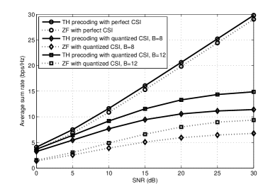
Figure 1: The average sum rate versus system SNR $P$ under $n_{T}=4$ and various $B$.

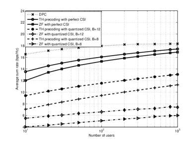
Figure 2: The average sum rate versus number of users $K$ under $n_{T}=4$, $P=15$ dB and various $B$.

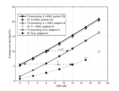
Figure 3: The average sum rate versus SNR $P$ under $n_{T}=4$, and adaptive $B$ or $K$ such that $B+\log_{2}K=(n_{T}-1)\log_{2}P+8.32$.

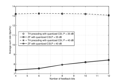
Figure 4: The average sum rate versus the number of feedback bits $B$ in high-SNR regime ($P=35$ dB, $P=40$ dB) under $n_{T}=4$, and adaptive $B$ or $K$ such that $B+\log_{2}K=16.55$.

Fig. 2 plots the average sum rate as a function of the number of users achieved by TH precoding and ZFBF based on both perfect CSI and quantized CSI at the transmitter side. A curve is also presented for the optimal DPC which acts as an achievable upper bound, and is computed using the algorithm from [11]. As evident from the figure, the average sum rate of TH precoding scheme with perfect CSI converges slowly to the average sum rate achieved with optimal DPC as $K$ grows large. The curves for the quantized CSI cases are far below those for the perfect CSI cases at finite $K$, which is due to MUI as explained in Section IV for TH precoding and in [17] for ZFBF, respectively. Still, we can see the trend of convergence to the optimal DPC for the quantized CSI case. In addition, TH precoding performs significantly better than linear ZFBF for both the perfect CSI and quantized CSI cases. For finite $K$, there is a gap between the average sum rates achieved by TH precoding and ZFBF for both the perfect CSI and quantized CSI cases. Moreover, the gap between the average sum rates achieved by TH precoding and ZFBF for the systems with quantized CSI increases as $K$ increases, whereas this gap in the systems with perfect CSI decreases as $K$ increases. In fact, we see that the curve for ZFBF with perfect CSI converges slowly to that of DPC (thus, converge to that of TH precoding) as $K$ grows large. However, the speed of convergence is slower than that of TH precoding. This result has also been proved in [22].

Fig. 3 investigates the interchangeability between $B$ and $\log_{2}K$, where we adapt $B$ and $K$ as

$$B-B_{0}+\log_{2}\left(\frac{K}{K_{0}}\right)=(n_{T}-1)\log_{2}\left(\frac{P}{P_{0}}\right),$$ (51)

so that a constant gap from the sum rate of the perfect CSI case can be maintained. We consider a system in the large-user regime such that $K_{0}=5000,B_{0}=6$, $P_{0}=10$ dB. This corresponds to $B+\log_{2}K=(n_{T}-1)\log_{2}P+8.32$. We either fix $K=K_{0}$ and adapt $B$ as a function of $P$, or fix $B=B_{0}$ and adapt $K$ as a function of $P$. For comparison, we plot the results for both TH precoding and ZFBF. We find that, in the large-user regime, the average sum rate achieved by TH precoding and ZFBF with perfect CSI are very close to each other, whereas the corresponding results with quantized CSI are very different. Particularly, we can observe a constant SNR gap of about $5$ dB from the perfect CSI curve for TH precoding, which confirms the analysis in Section IV. Whereas the corresponding SNR gap for ZFBF is about $11$ dB from the perfect CSI curve and this gap increases a little as SNR increases in the large-user regime.

Fig. 4 investigates the interchangeability between $B$ and $\log_{2}K$ in the high-SNR regime ($P=35$ dB, $P=40$ dB) for both TH precoding and ZFBF, where we adapt $B$ and $K$ as (51). We consider a system in the large-user high-SNR regime such that $K_{0}=3000,B_{0}=5$ and $P_{0}=P$. This corresponds to $B+\log_{2}K=16.55$. We adapt $K$ as a function of $B$. For comparison, we plot the results for both TH precoding and ZFBF. It is seen that the average sum rate achieved by TH precoding almost remains constant as $B$ increases, and also doesn’t change much as SNR increases from $35$ dB to $40$ dB, which aligns with the analysis in Section IV. However, the average sum rate of ZFBF increases a little as the number of feedback bits $B$ increases.

$$f(t_{1},\ldots,t_{n-1})=\left\{\begin{array}[]{ll}\frac{\Gamma(n_{T})}{\Gamma(n_{T}-n+1)}\left(1-\sum_{i=1}^{n-1}t_{i}\right)^{n_{T}-n},&t_{i}\geq 0,i=1,\ldots,n-1,\sum_{i=1}^{n-1}t_{i}\leq 1\\ 0,&\text{otherwise}\end{array}\right..$$ (54)

VI Conclusion

We have investigated the sum rate of a quantized CSI-based TH precoding scheme for a MU-MIMO system, denoted G-THP-Q. We have proved that for fixed finite SNR and finite $n_{T}$, G-THP-Q can achieve the optimal sum rate scaling of the MIMO broadcast channel, and that the average sum rate converges to the average sum capacity of the MIMO broadcast channel as the number of users $K$ grows large. In addition, our analytical results have provided important insights into the effect of quantized CSI on the multiuser diversity gain in both the first- and the second-order terms. We have studied and derived the tradeoffs between the number of feedback bits, the number of users and SNR. Particularly, a constant SNR gap from the result of the perfect CSI case can be achieved by simultaneously interchanging the number of users and feedback bits.

Appendix A Proof of Lemma 2

According to Lemma 1, for large $K$, the channel direction vector $\bar{\mathbf{h}}_{k}$, for $k\in\mathcal{U}_{n}$, is an isotropically distributed unit vector on the $n_{T}$-dimensional complex unit hypersphere. Using RVQ, the same results holds for the quantized channel direction vector $\hat{\mathbf{h}}_{k}$, for $k\in\mathcal{U}_{n}$. In addition, the subspace spanned by the orthonormal basis $\hat{\mathbf{q}}_{1},\ldots,\hat{\mathbf{q}}_{n-1}$ becomes independent of $\bar{\mathbf{h}}_{k}$, for $k\in\mathcal{U}_{n}$. Thus, without loss of generality we can assume $\mathbf{q}_{i}=\mathbf{e}_{i}$, where $\mathbf{e}_{i}$ is the $i$-th row of the identity matrix $\mathbf{I}_{n_{T}}$.

For $k\in\mathcal{U}_{n}$, let $\hat{\mathbf{h}}_{k}=[m_{1},\cdots,m_{n_{T}}]^{T}$, and $t_{i}=|\hat{\mathbf{h}}_{k}\hat{\mathbf{q}}_{i}^{H}|^{2}$. Then, with $\mathbf{q}_{i}=\mathbf{e}_{i},i=1,\ldots,n-1$, we have $t_{i}=|m_{i}|^{2}$ for $1\leq i\leq n-1$. The joint p.d.f. of $t_{1},\ldots,t_{n-1}$ has been obtained in [22] and is shown in (54) at the top of this page. Now we want to obtain the distribution of $w_{1}=\sum_{l=1}^{n-1}t_{l}$. We define the following transformation of variables

$$w_{1}=\sum_{l=1}^{n-1}t_{l},~{}~{}w_{i}=t_{i}~{}~{}~{}\text{for}~{}i=2,\ldots,n-1.$$ (55)

The corresponding Jacobian can be easily obtained as $J=1$. Thus the joint p.d.f. of $w_{1},\ldots,w_{n-1}$ is

$$f_{w_{1},\ldots,w_{n-1}}\left(x_{1},\ldots,x_{n-1}\right)$$

$$=\frac{\Gamma(n_{T})}{\Gamma(n_{T}-n+1)}\left(1-x_{1}\right)^{n_{T}-n}.$$ (56)

Since $0\leq t_{i}\leq 1$, we have $0\leq t_{1}=w_{1}-\sum_{i=2}^{n-1}w_{i}\leq 1$. According to (55), the region of the random variables after transformation can be obtained as $\mathcal{D}=\big{\{}\left(w_{1},\ldots,w_{n-1}\right)~{}|~{}0\leq\sum_{i=2}^{n-1}w_{i}\leq w_{1}\leq 1,0\leq w_{i}\leq 1~{}\text{for}~{}i=2,\ldots,n-1\big{\}}$. Then the marginal distribution of $w_{1}$ can be obtained as

$$f_{w_{1}}(x)$$

$$=\int\cdots\int_{\mathcal{D}}f(x,x_{2}\ldots,x_{n-1})~{}{\rm d}x_{2}\cdots{\rm d}x_{n-1}$$

$$=\int\cdots\int_{\mathcal{D}}\frac{\Gamma(n_{T})}{\Gamma(n_{T}-n)}\left(1-x_{1}\right)^{n_{T}-n}~{}{\rm d}x_{2}\cdots{\rm d}x_{n-1}$$

$$\mathop{=}\limits^{(a)}\frac{\Gamma(n_{T})}{\Gamma(n_{T}-n)}(1-x)^{n_{T}-n}\frac{x^{n-2}}{\left(n-2\right)!},$$

where in $(a)$ we have used the identity $\mathop{\int\int{\cdots\int{}}}\limits_{\scriptstyle\sum_{i=1}^{n}t_{i}\leq h\hfill\atop\scriptstyle t_{1}\geq 0,\ldots,t_{n}\geq 0\hfill}~{}{\rm d}t_{1}\cdots~{}{\rm d}t_{n}=\frac{h^{n}}{n!}$ [32]. We find that $w_{1}$ follows beta distribution with shape parameters $(n-1)$ and $(n_{T}-n+1)$. According to (20) we have $\omega_{k}(n)=1-\sum_{j}^{n-1}|\hat{\mathbf{h}}_{k}\hat{\mathbf{q}}_{j}^{H}|^{2}=1-w_{1}$. Thus $\omega_{k}(n)\sim\mathrm{Beta}(n_{T}-n+1,n-1)$, whose p.d.f. is given by (23).

Appendix B Proof of Lemma 4

From Lemma 3 it is clear that $\gamma_{k}(n)$ has the same distribution of $\gamma=\frac{\phi\omega\left(X+(1-\delta)Y\right)}{\phi\delta Y+1}$, where $\omega$ has the same distribution of $\omega_{k}(n)$, and $X,Y$ are defined in Lemma 3. Then we will derive the c.d.f. of $\gamma$ as

$$\mathrm{Pr}(\gamma\geq x)$$

$$=\mathrm{Pr}\left(\frac{\phi\omega\left(X+(1-\delta)Y\right)}{\phi\delta Y+1}\geq x\right)$$

$$=\int_{0}^{1}f_{\omega}(z){\rm d}z\int_{0}^{\infty}\mathrm{Pr}\left(X\geq\left(\frac{\delta}{z}y+\frac{1}{\phi z}\right)x-(1-\delta)y\right)$$

$$\hskip 28.45274pt\times f_{Y}(y){\rm d}y.$$ (57)

If $x\geq\frac{1-\delta}{\delta}$, then $\left(\frac{\delta}{z}y+\frac{1}{\phi z}\right)x-(1-\delta)y$ is nonnegative for any $y\geq 0$ and $0\leq z\leq 1$. Using the definition of random variables $X$ and $Y$, the above can be further written as

$$\mathrm{Pr}(\gamma\geq x)$$

$$=\int_{0}^{1}f_{\omega(n)}(z){\rm d}z\int_{0}^{\infty}e^{-\left(\frac{\delta}{z}y+\frac{1}{\phi z}\right)x+(1-\delta)y}f_{Y}(y){\rm d}y$$

$$=\int_{0}^{1}e^{-\frac{x}{\phi z}}f_{\omega}(z){\rm d}z\int_{0}^{\infty}e^{-\left[\frac{\delta}{z}x-(1-\delta)\right]y}\frac{y^{n_{T}-2}e^{-y}}{(n_{T}-2)!}{\rm d}y$$

$$=\int_{0}^{1}e^{-\frac{x}{\phi z}}f_{\omega}(z){\rm d}z\int_{0}^{\infty}\frac{e^{-\delta\left(\frac{x}{z}+1\right)y}y^{n_{T}-2}}{(n_{T}-2)!}{\rm d}y$$

$$=\int_{0}^{1}\frac{2^{B}e^{-\frac{x}{\phi z}}}{\left(\frac{x}{z}+1\right)^{n_{T}-1}}\frac{1}{\beta(n_{T}-n+1,n-1)}$$

$$\hskip 28.45274pt\times z^{n_{T}-n}(1-z)^{n-2}{\rm d}z$$

$$=c_{n}\int_{0}^{1}\frac{e^{-\frac{x}{\phi z}}}{\left(z+x\right)^{n_{T}-1}}z^{2n_{T}-n-1}(1-z)^{n-2}{\rm d}z,$$ (58)

where $c_{n}$ is as defined in the lemma statement.

With the change of variables $t=\frac{x}{z}$, (58) can be written as

$$\mathrm{Pr}(\gamma\geq x)$$

$$=c_{n}\int_{x}^{\infty}\frac{e^{-\frac{t}{\phi}}}{\left(\frac{x}{t}+x\right)^{n_{T}-1}}\left(\frac{x}{t}\right)^{2n_{T}-n-1}\left(1-\left(\frac{x}{t}\right)\right)^{n-2}$$

$$\hskip 56.9055pt\times\frac{x}{t^{2}}{\rm d}t$$

$$=c_{n}x^{n_{T}-n+1}\int_{x}^{\infty}e^{-\frac{t}{\phi}}\frac{(t-x)^{n-2}}{\left(t+1\right)^{n_{T}-1}t^{n_{T}}}{\rm d}t$$

$$=c_{n}x^{n_{T}-n+1}V(n-1;-n_{T}+2;-n_{T}+1;\frac{1}{\phi};x).$$ (59)

Thus Lemma 4 is proved.

Appendix C Proof of Lemma 5

Using the geometric-mean inequality we have

$$(t+1)^{n_{T}-1}t^{n_{T}} <\left(\frac{(n_{T}-1)(t+1)+{n_{T}}t}{2n_{T}-1}\right)^{2n_{T}-1}$$

$$=\left(t+\frac{n_{T}-1}{2n_{T}-1}\right)^{2n_{T}-1}.$$ (60)

Thus, for $\frac{1}{\delta}<x<\infty$,

$$V(n-1;-n_{T}+2;-n_{T}+1;\frac{1}{\phi};x)$$

$$>\int_{x}^{\infty}e^{-\frac{t}{\phi}}\frac{(t-x)^{n-2}}{\left(t+\frac{n_{T}-1}{2n_{T}-1}\right)^{2n_{T}-1}}{\rm d}t$$

$$=\int_{x+\frac{n_{T}-1}{2n_{T}-1}}^{\infty}e^{-\frac{s-\frac{n_{T}-1}{2n_{T}-1}}{\phi}}\frac{\left(s-x-\frac{n_{T}-1}{2n_{T}-1}\right)^{n-2}}{s^{2n_{T}-1}}~{}{\rm d}s$$ (61)

$$=e^{\frac{\frac{n_{T}-1}{2n_{T}-1}}{\phi}}\left(\frac{1}{\phi}\right)^{\frac{2n_{T}-n-1}{2}}\Gamma(n-1)$$

$$\hskip 14.22636pt\times\left(x+\frac{n_{T}-1}{2n_{T}-1}\right)^{\frac{n-2n_{T}-1}{2}}\exp\left(-\frac{x+\frac{n_{T}-1}{2n_{T}-1}}{2\phi}\right)$$

$$\hskip 14.22636pt\times W_{\frac{-2n_{T}-n+3}{2},\frac{2n_{T}-n}{2}}\left(\frac{x+\frac{n_{T}-1}{2n_{T}-1}}{\phi}\right)$$ (62)

$$=\Gamma(n-1)\left(\frac{1}{\phi}\right)^{\frac{2n_{T}-n-1}{2}}e^{\frac{\frac{n_{T}-1}{2n_{T}-1}}{2\phi}}$$

$$\hskip 14.22636pt\times\left(x+\frac{n_{T}-1}{2n_{T}-1}\right)^{-\frac{2n_{T}-n+1}{2}}\exp\left(-\frac{x}{2\phi}\right)$$

$$\hskip 28.45274pt\times W_{\frac{-2n_{T}-n+3}{2},\frac{2n_{T}-n}{2}}\left(\frac{x+\frac{n_{T}-1}{2n_{T}-1}}{\phi}\right),$$ (63)

where the change of variables $s=t+\frac{n_{T}-1}{2n_{T}-1}$ is employed in (61), whilst (C) is obtained by using [32, 3.383.4]. In addition, we have

$$V(n-1;-n_{T}+2;-n_{T}+1;\frac{1}{\phi};x)$$

$$<\int_{x}^{\infty}e^{-\frac{t}{\phi}}\frac{(t-x)^{n-2}}{t^{2n_{T}-1}}{\rm d}t$$

$$=\Gamma(n-1)\left(\frac{1}{\phi}\right)^{\frac{2n_{T}-n-1}{2}}x^{-\frac{2n_{T}-n+1}{2}}\exp\left(-\frac{x}{2\phi}\right)$$

$$\hskip 28.45274pt\times W_{\frac{-2n_{T}-n+3}{2},\frac{2n_{T}-n}{2}}\left(\frac{x}{\phi}\right),$$ (64)

where we have used [32, 3.383.4] again to obtain (C). Then, for $\frac{1}{\delta}<x<\infty$ and $n\geq 2$, $F_{\bar{\gamma}(n)}(x)$ and $F_{\tilde{\gamma}(n)}(x)$ are obtained by individually substituting (C) and (C) into (4) with $\Gamma(n-1)=(n-2)!$. In addition, it is easy to prove that $F_{\tilde{\gamma}(n)}(0)=0$, $F_{\tilde{\gamma}(n)}(1)=1$ and $F_{\tilde{\gamma}(n)}(x)$ is an increasing function of $x$. Thus, $F_{\tilde{\gamma}(n)}(x)$ is a distribution function. For the same reasons, $F_{\bar{\gamma}(n)}(x)$ is also a distribution function. Lemma 5 is proved.

Appendix D Asymptotic expansion of c.d.f.s of $\tilde{\gamma}_{k}(n)$ and $\bar{\gamma}_{k}(n)$ for large $x$.

Using the asymptotic expansion of the Whittaker function $W_{\lambda,\mu}(x)$ for large $x$ given by [32, 9.227], we have

$$W_{\frac{-2n_{T}-n+3}{2},\frac{2n_{T}-n}{2}}\left(\frac{x+\frac{n_{T}-1}{2n_{T}-1}}{\phi}\right)$$

$$=\exp\left(-\frac{x+\frac{n_{T}-1}{2n_{T}-1}}{2\phi}\right)\left(\frac{x+\frac{n_{T}-1}{2n_{T}-1}}{\phi}\right)^{\frac{-2n_{T}-n+3}{2}}$$

$$\hskip 28.45274pt\times\left(1+O\left(\frac{1}{x+\frac{n_{T}-1}{2n_{T}-1}}\right)\right)$$ (65)

and

$$W_{\frac{-2n_{T}-n+3}{2},\frac{2n_{T}-n}{2}}\left(\frac{x}{\phi}\right)$$

$$=\exp\left(-\frac{x}{2\phi}\right)\left(\frac{x}{\phi}\right)^{\frac{-2n_{T}-n+3}{2}}\left(1+O\left(\frac{1}{x}\right)\right).$$ (66)

Substituting (D) and (D) into (5) and (5) respectively, after some manipulations we obtain (IV) and (IV).

Appendix E Proof of Lemma 6

Applying the results in [24, Appendix I] to the distribution of $\tilde{\gamma}_{k}(n)$ in (5) with $a_{K,n}=\phi$ and $b_{K,n}=\phi\log\big{(}\frac{c_{n}K}{\phi^{n_{T}-1}}\big{)}-\phi(n_{T}+n-2)\log\log\big{(}\frac{c_{n}K}{\phi^{n_{T}-1}}\big{)}$, we have the asymptotic results (E) at the top of next page.

$$\lim_{K\rightarrow\infty}K\left(1-F_{\tilde{{\gamma}}(n)}(a_{K,n}x+b_{K,n})\right)=\lim_{K\rightarrow\infty}\frac{c_{n}\phi^{n-1}K\exp\left(-\frac{a_{K,n}x+b_{K,n}}{\phi}\right)}{\left(a_{K,n}x+b_{K,n}\right)^{n_{T}+n-2}}$$

$$\hskip 8.53581pt=\lim_{K\rightarrow\infty}\frac{c_{n}\phi^{n-1}K\exp\left[-x-\log\left(\frac{c_{n}K}{\phi^{n_{T}-1}}\right)+(n_{T}+n-2)\log\log\left(\frac{c_{n}K}{\phi^{n_{T}-1}}\right)\right]}{\left[\phi x+\phi\log\big{(}\frac{c_{n}K}{\phi^{n_{T}-1}}\big{)}-\phi(n_{T}+n-2)\log\log\big{(}\frac{c_{n}K}{\phi^{n_{T}-1}}\big{)}\right]^{n_{T}+n-2}}$$

$$\hskip 8.53581pt=\lim_{K\rightarrow\infty}\frac{e^{-x}\left(\log\left(\frac{c_{n}K}{\phi^{n_{T}-1}}\right)\right)^{n_{T}+n-2}}{\left[x+\log\big{(}\frac{c_{n}K}{\phi^{n_{T}-1}}\big{)}-(n_{T}+n-2)\log\log\big{(}\frac{c_{n}K}{\phi^{n_{T}-1}}\big{)}\right]^{n_{T}+n-2}}$$

$$\hskip 8.53581pt=e^{-x}.$$ (67)

Similarly, we can show that $\lim_{K\rightarrow\infty}K\left(1-F_{\bar{{\gamma}}(n)}(a_{K,n}x+b_{K,n})\right)=e^{-x}$. Borrowing the language from extreme value theory of order statistics, $F_{{{\tilde{\gamma}}}(n)}(x)$ and $F_{\bar{{\gamma}}(n)}(x)$ are in the domain of attraction of type (III) limiting distribution [24, Theorem 4]. The final results can be obtained by utilizing a similar method used in [24, Lemma 7].

Appendix F Proof of Lemma 7

Recall that $F_{{\tilde{\gamma}}_{\mathcal{S}(n)}}(x)\leq F_{{\gamma}_{\mathcal{S}(n)}}(x)\leq F_{{\bar{\gamma}}_{\mathcal{S}(n)}}(x)$. For $\gamma_{\mathcal{S}(n)},n\in\{2,\ldots,M\}$, and large $K$, with (6), $\text{Pr}\{\chi_{n}-\phi\log\log\sqrt{K}\leq\gamma_{\mathcal{S}(n)}\}\geq\text{Pr}\{\chi_{n}-\log\log\sqrt{K}\leq\bar{\gamma}_{\mathcal{S}(n)}\}\geq 1-O\bigg{(}\frac{1}{\log K}\bigg{)}$. Similarly, with (6) we have $\text{Pr}\{\gamma_{\mathcal{S}(n)}\leq\chi_{n}+\phi\log\log\sqrt{K}\}\geq\text{Pr}\{\tilde{\gamma}_{\mathcal{S}(n)}\leq\chi_{n}+\log\log\sqrt{K}\}\geq 1-O\bigg{(}\frac{1}{\log K}\bigg{)}$. Thus, (7) holds. For the case $n=1$, the asymptotic distribution of $\gamma_{\mathcal{S}(1)}$ is obtained in [17, Theorem 1] as

$$\text{Pr}\{\chi_{1}-\phi\log\log\sqrt{K}\leq\gamma_{\mathcal{S}(1)}$$

$$\leq\chi_{1}+\phi\log\log\sqrt{K}\}\geq 1-O\bigg{(}\frac{1}{\log K}\bigg{)}.$$ (68)

The lemma is proved by combining (7) and (F).

Appendix G Proof of Theorem 1

Using (7) we can obtain $\text{Pr}\bigg{\{}\frac{\log_{2}(1+\chi_{n}-\phi\log\log\sqrt{K})}{\log_{2}{[\varrho\log K]}}\leq\frac{\log_{2}(1+{\gamma}_{\mathcal{S}(n)})}{\log_{2}[\varrho\log K]}\leq\frac{\log_{2}(1+\chi_{n}+\phi\log\log\sqrt{K})}{\log_{2}{[\varrho\log K]}}\bigg{\}}\geq 1-O\bigg{(}\frac{1}{\log K}\bigg{)}$. Substituting (32) and (34) and letting $K\rightarrow\infty$, the left-hand side and the right-hand side inequality within $\text{Pr}\{\cdot\}$ converge to the same value. Thus, $\lim_{K\rightarrow\infty}\frac{\log_{2}(1+{\gamma}_{\mathcal{S}(n)})}{\log_{2}[\varrho\log K]}=1$ with probability 1, and (35) holds. To establish (36), we employ the upper bound on $\mathbb{E}\{R_{\text{BC}}\}$ derived in [35], which is given as $\mathbb{E}\{R_{\text{BC}}\}\leq n_{T}\log_{2}\big{(}1+\varrho(\log K+O(\log\log K))\big{)}$. From Lemma 7, we have $\text{Pr}\bigg{\{}\log_{2}(1+{\gamma}_{\mathcal{S}(n)})\geq\log_{2}(1+\chi_{n}-\phi\log\log\sqrt{K})\bigg{\}}\geq 1-O\bigg{(}\frac{1}{\log K}\bigg{)}$. Thus, we have (G) at the top of this page,

$$\mathbb{E}\{R_{\text{BC}}\}-\mathbb{E}\{R_{\text{G-THP-Q}}\}$$

$$\leq n_{T}\log_{2}\big{(}1+\varrho(\log K+O(\log\log K))\big{)}-\bigg{(}1-O\bigg{(}\frac{1}{\log K}\bigg{)}\bigg{)}\sum_{n=1}^{n_{T}}\log_{2}\big{(}1+\chi_{n}-\phi\log\log\sqrt{K}\big{)}$$

$$=\sum_{n=1}^{n_{T}}\log_{2}\big{(}\frac{1+\varrho(\log K+O(\log\log K))}{1+\chi_{n}-\phi\log\log\sqrt{K}}\big{)}+O\bigg{(}\frac{1}{\log K}\bigg{)}\sum_{n=1}^{n_{T}}\log_{2}\big{(}1+\chi_{n}-\phi\log\log\sqrt{K}\big{)}$$

$$\sim\sum_{n=1}^{n_{T}}\log_{2}\bigg{(}1+\frac{\frac{P}{Mn_{T}}\log K+O\left(\log\log{K}\right)+\phi\log\left(\frac{\phi^{n_{T}-1}}{c_{n}}\right)}{1+\frac{(M-1)P}{Mn_{T}}\log K+O\left(\log\log{K}\right)}\bigg{)}+O\bigg{(}\frac{1}{\log K}\bigg{)}O(\log\log K)$$

$$\sim\frac{n_{T}}{\log 2}\log\bigg{(}1+\frac{1}{M-1}+O\left(\frac{\log\log K}{\log K}\bigg{)}+O\left(\frac{1}{\log K}\right)\right)+O\bigg{(}\frac{\log\log K}{\log K}\bigg{)}.$$ (69)

where $x\sim y$ means $\lim_{K\rightarrow\infty}x/y=1$. Thus (36) is proved. Equation (38) is proved by combining (69) and the fact that $\log(1+x)\approx x$ for $x\ll 1$.

Appendix H Proof of Lemma 8

When $x\geq\frac{1}{\delta}-1$ and $\frac{x}{y}\geq\frac{1}{\delta}-1$, $y\leq\frac{x}{\frac{1}{\delta}-1}$ and $\frac{x}{\frac{1}{\delta}-1}\geq 1$. In addition, $\omega_{k}(n)$ and $Z\stackrel{{\scriptstyle\Delta}}{{=}}\frac{\cos^{2}\theta_{k}}{\sin^{2}\theta_{k}}$ are independent, thus the c.d.f. of $\hat{\gamma}_{k}(n)$ can be obtained as

$$F_{\hat{\gamma}(n)}(x)$$

$$=\int_{0}^{1}F_{Z}\bigg{(}\frac{x}{y}\bigg{)}f_{\omega(n)}(y){\rm d}y,$$

$$=\int_{0}^{1}\left(1-\frac{2^{B}}{\left(\frac{x}{y}+1\right)^{n_{T}-1}}\right)f_{\omega(n)}(y){\rm d}y$$

$$=1-\int_{0}^{1}\frac{2^{B}}{\left(\frac{x}{y}+1\right)^{n_{T}-1}}\frac{1}{\beta(n_{T}-n+1,n-1)}$$

$$\hskip 28.45274pt\times y^{n_{T}-n}(1-y)^{n-2}$$

$$=1-\frac{2^{B}}{\beta(n_{T}-n+1,n-1)}\int_{0}^{1}\frac{y^{2n_{T}-n-1}y^{n-2}}{(x+y)^{n_{T}-1}}{\rm d}y$$

$$=1-\frac{2^{B}\beta(2n_{T}-n,n-1)}{\beta(n_{T}-n+1,n-1)}\frac{1}{x^{n_{T}-1}}$$

$$\hskip 28.45274pt\times{}_{2}F_{1}\left(n_{T}-1,2n_{T}-n;2n_{T}-1;-\frac{1}{x}\right),$$ (70)

where to obtain the last line we have used [32, 3.197.3].

Appendix I Proof of Lemma 9

First, for $n=1$ the extremal distribution in (9) has been obtained in [17]. By applying (45) with the change of variables $\acute{\gamma}(n)=\left(\frac{2^{B}}{d_{n}}\right)^{\frac{1}{n_{T}-1}}\hat{\gamma}(n)-1$, we have

$$F_{\acute{\gamma}(n)}(x) =F_{\hat{\gamma}(n)}\left(\frac{x+1}{\left(\frac{2^{B}}{d_{n}}\right)^{\frac{1}{n_{T}-1}}}\right)$$

$$=1-\frac{2^{B}}{(1+x)^{n_{T}-1}}+O\left(\frac{1}{x}\right),$$ (71)

which is the same as the tail distribution of $F_{\hat{\gamma}(1)}(x)$. Using (9) we have

$$\text{Pr}\bigg{\{}\left(\frac{2^{B}K}{\log\sqrt{K}}\right)^{\frac{1}{n_{T}-1}}-1\leq\left(\frac{2^{B}}{d_{n}}\right)^{\frac{1}{n_{T}-1}}\hat{\gamma}_{\mathcal{S}(n)}-1$$

$$\hskip 14.22636pt\leq\left(2^{B}K\log\sqrt{K}\right)^{\frac{1}{n_{T}-1}}-1\bigg{\}}\geq 1-O\left(\frac{1}{\log K}\right).$$ (72)

Thus (9) follows.

References

- [1] İ. E. Telatar, “Capacity of multi-antenna Gaussian channels,” Europ. Trans. Commun., pp. 585–595, Nov.-Dec. 1999.
- [2] P. W. Wolniansky, G. J. Foschini, G. D. Golden, and R. A. Valenzuela, “V-BLAST: An architecture for realizing very high data rates over the rich-scattering wireless channel,” in Proc. URSI Int. Symposium on Signals, Systems, and Electronics, pp. 295–300, Pisa, Italy 1998.
- [3] T. Haustein, C. von Helmolt, E. Jorswieck, V. Jungnickel, and V. Pohl, “Performance of MIMO systems with channel inversion,” in Proc. 55th IEEE Veh. Technol. Conf., pp. 35–39, Birmingham, AL, May 2002.
- [4] M. Joham, K.Kusume, M. H. Gzara, and W. Utschick, “Transmit Wiener filter for the downlink of TDD DS-CDMA systems,” in Proc. IEEE 7th Symp. Spread-Spectrum Technol., Applicat., pp. 9–13, Prague, Czech Republic, Sep. 2002.
- [5] C. B. Peel, B. M. Hochwald, and A. L. Swindlehurst, “A vector-perturbation technique for near-capacity multiantenna multi-user communication - Part I: Channel inversion and regularization,” IEEE Trans. Commun., vol. 53, no. 1, pp. 195–202, Jan. 2005.
- [6] J. Yang and S. Roy, “Joint transmitter-receiver optimization for multi-input multi-output systems with decision feedback,” IEEE Trans. Inform. Theory, vol. 40, no. 5, pp. 1334–1347, Sep. 1994.
- [7] B. M. Hochwald, C. B. Peel, and A. L. Swindlehurst, “A vector-perturbation technique for near-capacity multiantenna multiuser communication - Part II: Perturbation,” IEEE Trans. Commun., vol. 53, no. 3, pp. 537–544, Mar. 2005.
- [8] C. Windpassinger, R. F. H. Fischer, T. Vencel, and J. B. Huber, “Precoding in multiantenna and multiuser communications,” IEEE Trans. Wireless Commun., vol. 3, no. 4, pp. 1305–1316, Jul. 2004.
- [9] R. F. H. Fischer, Precoding and Signal Shaping for Digital Transmission, 1st ed. USA: New York: Wiley, 2002.
- [10] H. Weingarten, Y. Steinberg, and S. Shamai (Shitz), “The capacity region of the Gaussian multiple-input multiple-output broadcast channel,” IEEE Trans. Inform. Theory, vol. 52, no. 9, pp. 3936–3964, Sep. 2006.
- [11] S. Vishwanath, N. Jindal, and A. Goldsmith, “Duality, achievable rates, and sum-rate capacity of Gaussian MIMO broadcast channels,” IEEE Trans. Inform. Theory, vol. 49, no. 10, pp. 2658–2668, Oct. 2003.
- [12] G. Caire and S. Shamai (Shitz), “On the achievable throughput of a multi-antenna Gaussian broadcast channel,” IEEE Trans. Inform. Theory, vol. 49, no. 7, pp. 1691–1706, Jul. 2003.
- [13] A. D. Dabbagh and D. J. Love, “Precoding for multiple antenna Gaussian broadcast channels with successive zero-forcing,” IEEE Trans. Signal Process., vol. 55, no. 7, pp. 3837–3850, Jul. 2007.
- [14] M. O. Damen, A. Chkeif, and J.-C. Belfiore, “Lattice code decoder for space-time codes,” IEEE Commun. Lett., vol. 4, pp. 161–163, May. 2000.
- [15] H. Harashima and H. Miyakawa, “Matched-transmission technique for channels with intersymbol interference,” IEEE Trans. Commun., vol. 20, pp. 774–780, Aug. 1972.
- [16] A. A. D’Amico, “Tomlinson-Harashima precoding in MIMO systems: A unified approach to transceiver optimization based on multiplicative Schur-convexity,” IEEE Trans. Signal Process., vol. 56, no. 8, pp. 3662–3677, Aug. 2008.
- [17] T. Yoo, N. Jindal, and A. Goldsmith, “Multi-antenna downlink channels with limited feedback and user selection,” IEEE J. Sel. Areas Commun., vol. 25, no. 7, pp. 1478–1491, Sep. 2007.
- [18] N. Jindal, “MIMO broadcast channels with finite-rate feedback,” IEEE Trans. Inform. Theory, vol. 52, pp. 5045–5060, Nov. 2006.
- [19] C. Xing, M. Xia, F. Gao, and Y.-C. Wu, “Robust transceiver with Tomlinson-Harashima precoding for amplify-and-forward MIMO relaying systems,” IEEE J. Sel. Areas Commun., vol. 30, no. 8, pp. 1370–1382, Sep. 2012.
- [20] P. M. Castro, M. Joham, L. Castedo, and W. Utschick, “Optimized CSI feedback for robust THP design,” in Proc. 41st Asilomar Conference on Signals, Systems and Computers (ACSSC), Nov. 2007.
- [21] I. Slim, A. Mezghani, and J. A. Nossek, “Quantized CDI based Tomlinson Harashima precoding for broadcast channels,” in Proc. IEEE Int. Conf. on Commun. (ICC), Jun. 2011, pp. 1–5.
- [22] L. Sun and M. R. McKay, “Eigen-based transceivers for the MIMO broadcast channel with semi-orthogonal user selection,” IEEE Trans. Signal Process., vol. 58, no. 10, pp. 5246–5261, Oct. 2010.
- [23] J. Wang, D. J. Love, and M. D. Zoltowski, “User selection with zero-forcing beamforming achieves the asymptotically optimal sum rate,” IEEE Trans. Signal Process., vol. 56, no. 8, pp. 3713–3726, Aug. 2008.
- [24] M. A. Maddah-Ali, M. Ansari, and A. K. Khandani, “Broadcast in MIMO systems based on a generalized QR decomposition: Signaling and performance analysis,” IEEE Trans. Inform. Theory, vol. 54, no. 3, pp. 1124–1138, Mar. 2008.
- [25] N. Jindal, “Antenna combining for the MIMO downlink channel,” IEEE Trans. Wireless Commun., vol. 7, no. 10, pp. 3834–3844, Oct. 2008.
- [26] R. D. Wesel and J. M. Cioffi, “Achievable rates for Tomlinson-Harashima precoding,” IEEE Trans. Inform. Theory, vol. 44, no. 2, pp. 824–831, Mar. 1998.
- [27] U. Erez and R. Zamir, “Achieving on the AWGN channel with lattice encoding and decoding,” IEEE Trans. Inform. Theory, vol. 50, no. 10, pp. 2293–2314, Oct. 2004.
- [28] T. Yoo and A. J. Goldsmith, “On the optimality of multi-antenna broadcast scheduling using zero-forcing beamforming,” IEEE J. Sel. Areas Commun., vol. 24, no. 3, pp. 528–541, Mar. 2006.
- [29] F. Khan, LTE for 4G Mobile Broadband: Air Interface Technologies and Performance, 1st ed. Cambridge, U.K.: Cambridge University Press, 2009.
- [30] G. Dimic and N. Sidiropoulos, “On the downlink beamforming with greedy user selection: Performance analysis and a simple new algorithm,” IEEE Trans. Signal Process., vol. 53, no. 10, pp. 3857–3868, Jul. 2005.
- [31] J. Wang, D. J. Love, and M. D. Zoltowski, A result on order statistics. [Online]. Available: http:// docs.lib.purdue.edu/ecetr/347, Tech. Rep., Purdue Univ., West Lafayette, IN, 2007.
- [32] I. S. Gradshteyn and I. M. Ryzhik, Table of Integrals, Series, and Products, 6th ed. New York: Academic, 2000.
- [33] J. Galambos, The Asymptotic Theory of Extreme Order Statistics, 2nd ed. Malabar, Florida, USA: Robert E. Krieger, 1987.
- [34] H. David and H. Nagaraja, Order Statistics, 3rd ed. New York: John Wiley and Sons, 2003.
- [35] M. Sharif and B. Hassibi, “On the capacity of MIMO broadcast channels with partial side information,” IEEE Trans. Inform. Theory, vol. 2, no. 21, pp. 506–522, Feb. 2005.