Shrinkage priors for linear instrumental
variable models with many instruments

Abstract.

This paper addresses the weak instruments problem in linear instrumental variable models from a Bayesian perspective. The new approach has two components. First, a novel predictor-dependent shrinkage prior is developed for the many instruments setting. The prior is constructed based on a factor model decomposition of the matrix of observed instruments, allowing many instruments to be incorporated into the analysis in a robust way.

Second, the new prior is implemented via an importance sampling scheme, which utilizes posterior Monte Carlo samples from a first-stage Bayesian regression analysis. This modular computation makes sensitivity analyses straightforward.

Two simulation studies are provided to demonstrate the advantages of the new method. As an empirical illustration, the new method is used to estimate a key parameter in macro-economic models: the elasticity of inter-temporal substitution. The empirical analysis produces substantive conclusions in line with previous studies, but certain inconsistencies of earlier analyses are resolved.

1. Introduction

This paper considers the practically important problem of how to undertake an instrumental variables analysis when the instrumental variables may be only weakly predictive of the endogenous regressor. This problem is illustrated via an applied problem from monetary policy theory: estimating the elasticity of inter-temporal substitution (EIS). The EIS is a central parameter in the theoretically optimal consumption rule. The weak instruments problem is addressed by including an array of instruments which—in aggregate—alleviate the weak instruments phenomenon. In adding these many auxiliary instruments, care must be taken to avoid over-fitting, which will be achieved through a powerful shrinkage prior based on ideas from factor analysis. Using Bayesian factor models for the purpose of inducing a regression can prove problematic (Hahn et al., 2013): if the dominant factor structure apparent in the instruments does not predict the endogenous regressor, estimates of the first stage regression can be strongly biased to zero, exacerbating the identification problem the instruments were intended to resolve. What is required instead is a prior over the first-stage regression coefficients which is biased towards any obvious factor structure, but which does not collapse sharply to zero if the evident structure in the instruments appears not to be predictive of the endogenous regressor. It is demonstrated that a prior built on this principle can be constructed in terms of an approximate low-rank decomposition of the instruments matrix. Finally, an importance resampling approach is developed to implement the new prior in the instrumental variables setting.

1.1. Overview

The balance of this paper introduces a factor shrinkage prior and explores its many relations to previous methods and its application to instrumental variable models with many instruments. Specifically, Section 2 lays out the background and notation of Bayesian linear IV, Gaussian linear factor models, and predictor-dependent priors for linear regression.

Despite this rich context, the basic intuition behind the new prior is quite straightforward, and is worth delineating at the outset. Begin with a linear model for a scalar response variable $x_{i}$:

$$x_{i}=\mathrm{z}^{t}_{i}\boldsymbol{\delta}+\epsilon_{i};\;\;\;\;\epsilon_{i}\operatorname{\stackrel{{\scriptstyle\mbox{\tiny iid}}}{{\sim}}}\mbox{N}(0,\sigma^{2}).$$

A factor shrinkage prior over the vector of regression coefficients $\boldsymbol{\delta}$ is induced via the following three steps.

1. First, suppose that $\mbox{cov}(\mathrm{z})=\mathbf{B}\mathbf{B}^{t}+\boldsymbol{\Psi}^{2}$ is known, for $\boldsymbol{\Psi}^{2}$ diagonal and $\mbox{rank}(\mathbf{B})\ll\mbox{dim}(\mathrm{z})$. That is, suppose that the factor structure of the predictor variables is known.

2. Next, create an over-complete dictionary by decomposing $\mathbf{Z}$ into i) its projection onto the column space of $\mathbf{B}$ and ii) the residuals arising from this projection. Specifically, define $\tilde{\mathbf{Z}}=\begin{pmatrix}\tilde{\mathbf{B}}^{t}\mathbf{Z}\\ (\mathbf{I}-\tilde{\mathbf{B}}\tilde{\mathbf{B}}^{t})\mathbf{Z}\end{pmatrix},$ where $\tilde{\mathbf{B}}$ is an orthonormalization of $\mathbf{B}$. Note that the span of $\tilde{\mathbf{Z}}$ is the same as for $\mathbf{Z}$.

3. Redefine the likelihood in terms of $\tilde{\mathrm{z}}$: $x_{i}=\tilde{\mathrm{z}}^{t}_{i}\tilde{\boldsymbol{\delta}}+\epsilon_{i}\;\;\;\;\epsilon_{i}\operatorname{\stackrel{{\scriptstyle\mbox{\tiny iid}}}{{\sim}}}\mbox{N}(0,\sigma^{2}).$ Proceed with Bayesian inference under one’s preferred shrinkage prior over $\tilde{\boldsymbol{\delta}}$.

The intuition behind this method is simply that if the derived variables $\tilde{\mathbf{B}}^{t}\mathbf{Z}$ are strong predictors of $x$, the shrinkage prior on $\tilde{\boldsymbol{\delta}}$ should allow to spot this strong signal; at the same time, if these derived variables are not by themselves adequate, the residual predictors $(\mathbf{I}-\tilde{\mathbf{B}}\tilde{\mathbf{B}}^{t})\mathbf{Z}$ have still been retained. In the former case, one has relied on the factor structure of the predictor variables to construct an approximately sparse regression problem with $p+k$ predictors, of which $k$ are dominant. In the latter case, one has only added $k\ll p$ predictors and so one is essentially not much worse off than if fitting the unmodified regression.

This sketch has omitted many details. For example, in practice, the factor structure is not known exactly and so must be inferred or approximated and one must choose what prior to use once $\tilde{\mathbf{Z}}$ and $\tilde{\boldsymbol{\delta}}$ have been defined. Section 3 fills in these details and demonstrates the prior’s performance via a small simulation study. Finally, one must determine how to implement this prior within an instrumental variable analysis; Section 4 introduces an efficient importance sampler for this purpose.

Section 5 then turns to the empirical analysis and Section 6 concludes with a brief discussion.

2. Background

2.1. The Bayesian linear instrumental variables model

This section describes a simple re-parametrization of the usual Gaussian instrumental variables (IV) model. This representation will underpin the computational approach taken later.

The starting point of Bayesian approaches to endogenous regressors is the structural equation model

(1) $$\begin{split}y_{i}&=\beta x_{i}+\epsilon_{y}\\ x_{i}&=\mathrm{z}_{i}^{t}\boldsymbol{\delta}+\epsilon_{x}.\end{split}$$

where $(\epsilon_{x},\epsilon_{y})$ are jointly Gaussian with mean zero and covariance

$$\mbox{cov}\begin{pmatrix}\epsilon_{x}\\ \epsilon_{y}\end{pmatrix}\equiv\mathbf{S}=\begin{pmatrix}\sigma_{x}^{2}&\sigma_{xy}\\ \sigma_{yx}&\sigma_{y}^{2}\end{pmatrix}.$$

The variable $x_{i}$ is referred to as the treatment variable, $y_{i}$ is the response variable and $\mathrm{z}_{i}$ is a vector of instruments. The unknown parameters in this model are $\beta$, $\delta$, $\sigma_{x}^{2}$, $\sigma_{y}^{2}$ and $\sigma_{xy}=\sigma_{yx}$; the parameter of interest is $\beta$. Because of the implied covariance between $x_{i}$ and $\epsilon_{y}$, valid estimates of $\beta$ cannot be obtained from just a regression of $y_{i}$ onto $x_{i}$.

The joint distribution of the observables can be found by substitution

(2) $$\begin{split}x_{i}&=\mathrm{z}_{i}^{t}\boldsymbol{\delta}+\epsilon_{x},\\ y_{i}&=\mathrm{z}_{i}^{t}\boldsymbol{\delta}\beta+\beta\epsilon_{x}+\epsilon_{y}.\end{split}$$

A further reparametrization yields

(3) $$\begin{split}x_{i}&=\mathrm{z}_{i}^{t}\boldsymbol{\delta}+\nu_{x},\\ y_{i}&=\mathrm{z}_{i}^{t}\boldsymbol{\delta}\beta+\nu_{y},\end{split}$$

with

$$\mbox{cov}\begin{pmatrix}\nu_{x}\\ \nu_{y}\end{pmatrix}=\boldsymbol{\Omega}=\mathbf{A}\mathbf{S}\mathbf{A}^{t}$$

where $\mathbf{A}=\begin{pmatrix}1&0\\ \beta&1\end{pmatrix}$. Equation (3) is referred to as the “reduced form” equations, in contrast to (1), the “structural” equations. These various formulations invite a host of possible prior specifications. For a discussion of common specifications, see Lopes and Polson (2014).

The focus in this paper will be on priors for $\boldsymbol{\delta}$ when the number of instruments $p$ is large relative to the number of available observations $n$. Priors over the remaining parameters are determined by a factorization of the likelihood based on $\epsilon_{y}\mid\epsilon_{x}\sim\mbox{N}(\alpha\epsilon_{x},\xi^{2})$, where

(4) $$\alpha=\frac{\sigma_{y}}{\sigma_{x}}\rho;\;\;\;\xi^{2}=(1-\rho^{2})\sigma_{y}^{2},\\$$

with $\rho\equiv\frac{\sigma_{xy}}{\sigma_{x}\sigma_{y}}$. The matrix $\Omega$ can be written in terms of $\beta$, $\alpha$, $\xi^{2}$ and $\sigma_{x}^{2}$,

(5) $$\Omega=\begin{pmatrix}\sigma^{2}_{x}&(\beta+\alpha)\sigma_{x}^{2}\\ (\beta+\alpha)\sigma_{x}^{2}&(\beta+\alpha)^{2}\sigma_{x}^{2}+\xi^{2}\end{pmatrix},$$

which in turn corresponds to the following factorization of the joint likelihood over observables $(x,y)$:

(6) $$\begin{split}f(x,y\mid\mathrm{z})&=f(y\mid x,\mathrm{z})f(x\mid\mathrm{z})\\ &=\mbox{N}_{y\mid x}(x\beta+\alpha(x-\mathrm{z}^{t}\boldsymbol{\delta}),\xi^{2})\times\\ &\;\;\;\;\;\mbox{N}_{x}(\mathrm{z}^{t}\boldsymbol{\delta},\sigma_{x}^{2}).\end{split}$$

The appearance of $\boldsymbol{\delta}$ in both factors on the right-hand side means that observations of $(y_{i},\mathrm{z}_{i})$ allow one to disentangle $\beta$ and $\alpha$. It is concievable, of course, that in a given applied problem one instead has

(7) $$f(x,y\mid\mathrm{z})=f(y\mid x,\mathrm{z})f(x\mid\mathrm{z})=\mbox{N}_{y\mid x}(x\beta+\alpha(x-\mathrm{z}^{t}\boldsymbol{\delta}),\xi^{2})\mbox{N}_{x}(\mathrm{z}^{t}\tilde{\boldsymbol{\delta}},\sigma_{x}^{2}),$$

with $\tilde{\boldsymbol{\delta}}\neq\boldsymbol{\delta}$. The assumption that $\tilde{\boldsymbol{\delta}}=\boldsymbol{\delta}$ is referred to as the instrument exclusion restriction and in general is untestable. See Conley et al. (2012) and Chan and Tobias (2014) for approaches which weaken this assumption, yielding only partial identification of $\beta$. In this paper, the exclusion restriction will be assumed.

Bayesian linear IV has been studied for many years now (Lindley and El-Sayed, 1968; Dreze, 1976; Geweke, 1996; Chamberlain and Imbens, 1996; Chao and Phillips, 1998) and remains an active area of research (Kleibergen and Zivot, 2003). For a textbook treatment, chapter 7 of Rossi et al. (2006) is a nice resource. The basic approach outlined above can be modified to consider non-Gaussian error terms (Conley et al., 2008). In the empirical illustration considered in Section 5, $y_{i}$ is the quarterly change in consumption in the United States, $x_{i}$ is the real interest rate and $\beta$ denotes the elasticity of inter-temporal substitution. The instrument vector $\mathrm{z}_{i}$ consists of a battery of macroeconomic indicators, twice-lagged. This formulation of the economic problem follows from a linearization of an Euler equation; see Yogo (2004) section II (and references therein) for details.

2.2. Gaussian factor regression models

Given a $p$-by-$k$ matrix $\mathbf{B}$ and a $k$-by-$1$ vector $\mathrm{f}_{i}$, a linear factor model for the $p$-dimensional vector $\mathrm{z}_{i}$ takes the form

(8) $$\mathrm{z}_{i}=\mathbf{B}\mathrm{f}_{i}+\epsilon_{i}$$

where $\epsilon_{i}$ is a $p$-dimensional, independent, additive error term (referred to as idiosyncratic errors). Conditional on the factors $\mathrm{f}_{i}$, the data may be viewed as realizations of an independent and identically distributed random variable. However, the latent factor scores $\mathrm{f}_{i}$ are not observable, rather they are given a prior distribution. Integrating over the latent factors induces a dependence structure among the observed data, in particular

(9) $$\mbox{Cov}(\mathrm{z}_{i})=\mathbf{B}\mbox{Cov}(\mathrm{f}_{i})\mathbf{B}^{t}+\boldsymbol{\Psi}^{2},$$

where $\mbox{Cov}(\epsilon_{i})=\boldsymbol{\Psi}^{2}$ is assumed diagonal.

When the priors over the latent factors and the idiosyncratic errors are both Gaussian, $\mathrm{f}_{i}\operatorname{\stackrel{{\scriptstyle\mbox{\tiny iid}}}{{\sim}}}\mbox{N}(0,\mathbf{I}_{k})$ and $\epsilon_{i}\operatorname{\stackrel{{\scriptstyle\mbox{\tiny iid}}}{{\sim}}}\mbox{N}(0,\boldsymbol{\Psi}^{2})$, the marginal distribution of $\mathrm{z}_{i}$ is also normally distributed,

(10) $$\mathrm{z}_{i}\sim\mbox{N}(0,\mathbf{B}\mathbf{B}^{t}+\boldsymbol{\Psi}^{2}),$$

and the model is called a Gaussian factor model.

Factor models have been a topic of research for more than 100 years. A seminal reference is Spearman (1904) and Bartholomew and Moustaki (2011) is an excellent contemporary reference. Bayesian factor models continue to see new developments, for example Lopes et al. (2008) and Murray et al. (2013). Recent work considering the use of factor models in the many instruments context include Groen and Kapetanios (2009); Ng and Bai (2009); Hahn and Hansen (2011) and Kapetanios and Marcellino (2010). Much of this previous work on factor models for IV analysis is non-Bayesian and the Bayesian treatments tend to focus specifically on asymptotic analysis under non-informative priors. The present paper differs from these earlier approaches in considering predictor dependent priors and an importance sampling implementation.

2.2.1. Weak factors and weak instruments

Factor models can be useful in a regression context owing to their ability to leverage “side information”. To observe this phenomenon, consider a factor regression model specified as:

(11) $$x_{i}=\mathrm{z}^{t}_{i}\boldsymbol{\delta}+\epsilon_{i};\;\;\;\ \epsilon_{i}\sim\mbox{N}(0,\sigma^{2});\;\;\;\boldsymbol{\delta}=\boldsymbol{\theta}\mathbf{B}^{t}(\mathbf{B}\mathbf{B}^{t}+\boldsymbol{\Psi}^{2})^{-1}.$$

Suppose that $\mathrm{z}_{i}$ follows the distribution in (10) and that many observations are available from this distribution, whereas only a limited number of $x$ observations are available. In this case, inference concerning $\boldsymbol{\delta}$ still benefits, because the “unlabeled” draws from (10) permit reliable inference concerning $\mathbf{B}$ and $\boldsymbol{\Psi}^{2}$, which reduces the $p$-dimensional regression in (11) to the problem of learning the $k$-dimensional vector $\theta$. (For a more general discussion of this idea, see Liang et al. (2007).)

However, if the assumption in (11) relating $\boldsymbol{\delta}$ to $\mathbf{B}$ and $\boldsymbol{\Psi}^{2}$ fails, the factor regression strategy can backfire, leading to insidious bias; in particular the true but unknown $\boldsymbol{\delta}$ need not live in the span of $\mathbf{B}^{t}(\mathbf{B}\mathbf{B}^{t}+\boldsymbol{\Psi}^{2})^{-1}$. Inferences made under an incorrect assumption of this form tend to exhibit a strong zero-bias when priors on $\boldsymbol{\theta}$ are centered at the origin. A similar phenomenon has long been recognized in the area of principal component analysis, where it is referred to as the “least eigenvalue problem” (Jolliffe, 1982; Cox, 1968). The illustration of this weak factor problem in the Bayesian linear factor model context is the topic of Hahn et al. (2013).

In the IV context, the weak factor problem relates intimately to the “weak instrument” problem. Note that when $\boldsymbol{\delta}=0$ the likelihood in (4) is non-unique in terms of the parameters $\beta$ and $\alpha$, with any combination having the same sum $\beta+\alpha$ giving equivalent likelihood evaluations. The weak instruments problem refers then to cases where $\boldsymbol{\delta}$ is small (but not zero), so that the likelihood is nearly flat for many combinations of $\alpha$ and $\beta$. Therefore, strong zero-bias in $\boldsymbol{\delta}$ due to the weak factor problem will directly impact inferences concerning $\beta$ by inducing a weak instrument scenario. A natural way to avoid this difficulty is to work with a “pure regression model”, dealing only with a conditional model for $(x_{i}\mid\mathrm{z}_{i})$ rather than for $(x_{i},\mathrm{z}_{i})$ jointly. It is therefore natural to ask how evident structure in the predictor matrix might be incorporated into a prior of the regression coefficients.

In the applied context of this paper, factor structure in the instrument vector is plausible if one posits macroeconomic trends underlying joint movement of the various indicators.

2.3. Predictor-dependent priors

The idea of specifying a prior distribution over a set of regression coefficients in a way that depends on the observed matrix of predictor variables goes back at least to Zellner (1986), where the so-called $g$-prior was introduced:

(12) $$(\boldsymbol{\delta}\mid\sigma^{2},g)\sim\mbox{N}(0,g\sigma^{2}(\mathbf{Z}\mathbf{Z}^{t})^{-1}).$$

The $g$-prior continues to be a popular choice in the Bayesian variable selection literature (Liang et al., 2008; Maruyama and George, 2011), due largely to the convenient closed form marginal likelihood it implies. The $g$-prior can be motivated by specifying a regression problem in the de-correlated predictor space and using independent priors in that representation. That is, supposing $\mbox{cov}(\mathrm{z})\equiv\boldsymbol{\Sigma}=\mathbf{L}\mathbf{L}^{t}$ is known and defining $\mathrm{w}_{i}\equiv\mathbf{L}^{-1}\mathrm{z}_{i}$ gives that

(13) $$\mathrm{w}_{i}\sim\mbox{N}(0,\mathbf{I});\;\;\;x_{i}\sim\mbox{N}(\mathrm{w}_{i}^{t}\boldsymbol{\eta},\sigma^{2});\;\;\;\boldsymbol{\eta}\sim\mbox{N}(0,g\mathbf{I}),$$

implies

(14) $$x_{i}\sim\mbox{N}(\mathrm{z}_{i}^{t}\boldsymbol{\delta},\sigma^{2});\;\;\;\boldsymbol{\delta}=\mathbf{L}^{-t}\boldsymbol{\eta};\;\;\;\boldsymbol{\delta}\sim\mbox{N}(0,g\boldsymbol{\Sigma}^{-1}).$$

Zellner’s $g$-prior follows from using an empirical plug-in estimate of $\boldsymbol{\Sigma}^{-1}$. The general idea of working in a rotated predictor representation has been fruitful in many contexts, for example in a model averaging capacity (Clyde et al., 1996). West (2003) introduces generalized-singular $g$-priors as a way to formally tie factor models to principal component regression, essentially by letting the prior on each $\psi_{j}^{2}$ approach a degenerate distribution at 0, so that “the latent factors explain essentially all the variation in the predictors”. With no additive error, the observed data is assumed to arise as $\mathbf{Z}=\mathbf{B}\mathbf{F}$ and $\mathbf{B}$ can be computed (non-uniquely) via a generalized inverse. (In practice the eigenvalues of $\mathbf{B}$ will all be positive, but small values are set to zero.)

While West (2003) expresses concern that “a basic modelling issue arises from the explicit design-, and sample size-, dependence of the empirical factor model,” the insight connecting factor models and $g$-priors can be applied “in reverse” to ask: is it possible to specify a predictor-dependent prior that allows for non-zero idiosyncratic variances? That is, instead of using a dimension reduced design matrix based on the singular-value decomposition (SVD) of $\mathbf{Z}$, it should be possible to use a true factor decomposition of $n^{-1}\mathbf{Z}\mathbf{Z}^{t}$. Such a prior would benefit from the substantive bias that the response variable should associate more strongly with the communalities than the idiosyncratic errors, while directly avoiding the “weak factor” problem by working with a pure regression model rather than a joint model.

The next section lays out the mechanics of producing such a decomposition and describes how to use this decomposition to construct a robust factor shrinkage prior.

3. Factor shrinkage priors

If it were possible to extract latent factors governing the correlation structure in a vector of instruments, one might suppose that these factors would make “strong” instruments. However, such an approach is at risk of extracting the “wrong” latent factors with respect to the desired regression, which could worsen the weak instruments problem. This section builds a prior designed to nudge the regression towards apparent factor structure in the instruments matrix, without committing to the assumption that the endogenous regressor is independent of the instruments conditional on the factors.

The new factor shrinkage prior is built on two ideas, the Frisch decomposition of a matrix and a robust shrinkage prior called the horseshoe prior. Sections 3.1 and 3.2 provide the details of this work. Section 3.3 defines the new prior and section 3.4 conducts a small simulation study.

3.1. The Frisch decomposition

The notion of “shared factors” among vectors of measurements can be characterized in terms of an optimization problem motivated by the early work of Ragnar Frisch on “confluence analysis” (Frisch, 1934). Specifically, given a covariance matrix $\boldsymbol{\Sigma}$, consider the following rank minimization problem:

(15) $$\begin{split}\mbox{min}_{\mathbf{D}}&\;\;\;\;\mbox{rank}(\boldsymbol{\Sigma}-\mathbf{D})\\ \mbox{s.t.}&\;\;\;\;\mathbf{D}\mbox{ diagonal},\\ &\;\;\;\;\boldsymbol{\Sigma}-\mathbf{D}\geq 0.\end{split}$$

If $\mathbf{D}^{*}$ is a solution to (15), denote a matrix pair $(\boldsymbol{\Psi}^{2},\mathbf{B})$ a Frisch decomposition of $\boldsymbol{\Sigma}$, if

(16) $$\boldsymbol{\Psi}^{2}=\mathbf{D}^{*};\;\;\;\mathbf{B}\mathbf{B}^{t}=\boldsymbol{\Sigma}-\mathbf{D}^{*}.$$

By assuming $\boldsymbol{\Sigma}$ known, this problem is non-statistical in nature, yet it readily captures an intuition about what makes factor models appealing as descriptions of data. Factor models are popular not merely because they decomposes covariance structure into a common component and an independent (diagonal) component, but because it is anticipated that this decomposition can be done parsimoniously. Indeed, any $p$-by-$p$ covariance matrix has a $p-1$ dimensional factor representation (let $\boldsymbol{\Psi}^{2}=\iota_{p}\mathbf{I}$ for $\iota_{p}$ the smallest eigenvalue of the SVD), whereas the Frisch decomposition demands that we have the most concise of all such descriptions.

Alas, solving (15) is quite difficult. Fortunately, high quality approximations are available using a surrogate objective function based on the matrix trace (Fazel, 2002):

(17) $$\begin{split}\mbox{min}_{\mathbf{D}}&\;\;\;\;\mbox{trace}(\boldsymbol{\Sigma}-\mathbf{D})\\ \mbox{s.t.}&\;\;\;\;\mathbf{D}\mbox{ diagonal},\\ &\;\;\;\;\boldsymbol{\Sigma}-\mathbf{D}\geq 0.\end{split}$$

The trace approximation is convex and can be routinely solved by readily available software (Grant and Boyd, 2013, 2008). The specifics of this approximation are beyond the scope of this paper; see Ning et al. (2013) for an excellent overview with many references. The trace approximation serves to extract a “sharper” set of eigenvectors, in the sense of having a more rapidly decaying set of eigenvalues, as seen in Figure 1, which overlays the eigenvalues of an example covariance matrix $\boldsymbol{\Sigma}$ and $\boldsymbol{\Sigma}-\mathbf{D}^{*}$, where $\mathbf{D}^{*}$ solves (17). In this sense, the trace heuristic still isolates “commonalities”. Henceforth, whenever a Frisch decomposition is referred to, it is to be understood that it is computed approximately using the feasible trace formulation in (17).

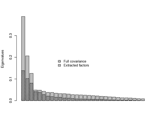
Figure 1. An illustration of how the eigenvalues of a full covariance matrix $\boldsymbol{\Sigma}$ can be flatter than the eigenvalues of the trace-heuristic derived loadings matrix $\boldsymbol{\Sigma}-\mathbf{D}^{*}$ . This occurs when $\boldsymbol{\Sigma}$ has an underlying factor structure with relatively large idiosyncratic variances.

3.2. The horseshoe prior

The “horseshoe” prior of Carvalho et al. (2010) is defined as a scale mixture of normals, with representation

(18) $$\pi(\delta_{j})=\int{\mbox{N}(\delta_{j}|0,\lambda_{j}^{2})\pi(\lambda_{j}^{2})}d\lambda_{j}.$$

To motivate this representation, consider the “intercept only model”, $(z_{j}\mid\delta_{j})\sim\mbox{N}(\delta_{j},1)$. Then, for $(\delta_{j}\mid\lambda_{j})\sim\mbox{N}(0,\lambda_{j}^{2})$, the posterior mean of $\delta_{j}$ may be expressed as

(19) $$\mbox{E}(\delta_{j}\mid z_{j})=\{1-\mbox{E}(\kappa_{j}\mid z_{j})\}z_{j},$$

where $\kappa_{j}=1/(1+\lambda_{j}^{2})$. The prior gets its name from the fact that a half-Cauchy prior $\lambda_{j}\sim\mbox{C}^{+}(0,1)$ yields a U-shaped $\mbox{Beta}\left(\frac{1}{2},\frac{1}{2}\right)$ distribution over the “shrinkage factor” $\kappa$, expressing the anticipation that shrinkage ought to be either severe ($\kappa\approx 1$) or minimal ($\kappa\approx 0$), and less likely to be at intermediate levels ($\kappa\approx 1/2)$.

The horseshoe and its relatives (such as Griffin and Brown (2012) and Polson and Scott (2012)) make good default priors for regression coefficients because they lack hyper-parameters and have been observed empirically to successfully shrink irrelevant coefficients strongly to zero without similarly attenuating the magnitude of relevant coefficients.

3.3. A factor shrinkage horseshoe prior

The factor shrinkage horseshoe prior arises as the implied prior on $\boldsymbol{\delta}$ when a horseshoe prior is placed on the regression coefficients corresponding to an augmented predictor matrix. This enriched predictor matrix is constructed using the Frisch decomposition of $\hat{\boldsymbol{\Sigma}}=n^{-1}\mathbf{Z}\mathbf{Z}^{t}$ (the hat denoting that this can be thought of as a point estimate of $\mbox{cov}(\mathrm{z})=\boldsymbol{\Sigma}$). The enriched predictor set is defined as follows. Let $(\mathbf{B},\boldsymbol{\Psi}^{2})$ denote the Frisch decomposition of $\hat{\boldsymbol{\Sigma}}$ and denote by $k$ the rank of $\mathbf{B}$. Let $\tilde{\mathbf{B}}$ denote the orthonormalization of $\mathbf{B}$. The enriched matrix is then defined as

(20) $$\tilde{\mathbf{Z}}=\begin{pmatrix}\tilde{\mathbf{B}}^{t}\mathbf{Z}\\ (\mathbf{I}-\tilde{\mathbf{B}}\tilde{\mathbf{B}}^{t})\mathbf{Z}\end{pmatrix}.$$

Note that $\tilde{\mathbf{Z}}$ is dimension $(p+k)$-by-$n$. Complete the regression model via

(21) $$\begin{split}x_{i}&=\tilde{\mathrm{z}}^{t}_{i}\tilde{\boldsymbol{\delta}}+\epsilon_{i}\;\;\;\;\epsilon_{i}\operatorname{\stackrel{{\scriptstyle\mbox{\tiny iid}}}{{\sim}}}\mbox{N}(0,\sigma^{2})\\ \tilde{\boldsymbol{\delta}}&\sim\mbox{N}(0,s^{2}\boldsymbol{\Lambda}^{2}),\;\;\;\lambda_{j}\sim\mbox{C}^{+}(0,1),\;\;\;s\sim\mbox{C}^{+}(0,1).\end{split}$$

The matrix $\boldsymbol{\Lambda}$ is diagonal with local shrinkage factors $\lambda_{j}$, $j=1,\dots,p+k$. Denote by $\boldsymbol{\Lambda}_{f}$ the upper $k$-by-$k$ block of $\boldsymbol{\Lambda}$, associated with the derived factors, and $\boldsymbol{\Lambda}_{r}$ the lower $p$-by-$p$ block associated with the residuals.

3.3.1. Local shrinkage and over-complete dictionaries

It may appear that nothing has been gained via working with the augmented design matrix. Indeed, the implied prior over $\boldsymbol{\delta}$ under (20) is mostly similar to a typical regression prior. In the special case where $\Lambda_{f}=\mathbf{I}_{k}$ and $\Lambda_{r}=\mathbf{I}_{p}$ are considered fixed, the prior on $\boldsymbol{\delta}$ is simply a standard normal:

(22) $$\begin{split}\mathbf{Z}^{t}\boldsymbol{\delta}&=\mathbf{Z}^{t}\tilde{\mathbf{B}}\tilde{\boldsymbol{\delta}}_{f}+\mathbf{Z}^{t}(\mathbf{I}-\tilde{\mathbf{B}}\tilde{\mathbf{B}}^{t})\tilde{\boldsymbol{\delta}}_{r},\\ \boldsymbol{\delta}&=\tilde{\mathbf{B}}\tilde{\boldsymbol{\delta}}_{f}+(\mathbf{I}-\tilde{\mathbf{B}}\tilde{\mathbf{B}}^{t})\tilde{\boldsymbol{\delta}}_{r},\\ \boldsymbol{\delta}&\sim\mbox{N}(0,\tilde{\mathbf{B}}\tilde{\mathbf{B}}^{t}+(\mathbf{I}-\tilde{\mathbf{B}}\tilde{\mathbf{B}}^{t})(\mathbf{I}-\tilde{\mathbf{B}}\tilde{\mathbf{B}}^{t})^{t})=\mbox{N}(0,\mathbf{I}).\end{split}$$

The last line follows from the idempotence of $\mathbf{I}-\tilde{\mathbf{B}}\tilde{\mathbf{B}}^{t}$.

However, the models are in fact quite different when the local hyper-variances are taken into account. The over-parametrized augmented matrix $\tilde{\mathbf{Z}}$ allows an expansion of what it means to be “local”, by creating new composite predictors that are themselves linear combinations of the original predictors. In this enriched set, the composite predictors may be found to represent the large signals, allowing more of the original predictor coefficients to be severely zero-shrunk.

The factor shrinkage prior construction suggests that local shrinkage priors combined with over-complete dictionaries could be a powerful general method for constructing novel priors for regression models.

3.3.2. Computational details

For completeness, note two additional details concerning the implemented Frisch decomposition. First, the solution to (15) is invariant to row and column scaling operations, while (17) is not. This observation has motivated weighted minimum trace approximations that attempt to define and compute an optimal weight matrix (Shapiro, 1982; Ning et al., 2013). As a crude heuristic, the approach taken here is to solve (17) applied to the sample correlation matrix as opposed to the sample covariance matrix.

Similarly, because $\boldsymbol{\Sigma}$ is only known up to an empirical estimate, the actual rank of $\mathbf{B}$ will tend not to be reduced. Accordingly, $\tilde{\mathbf{Z}}$ is constructed by approximating $\mathbf{B}$ (respectively, $\tilde{\mathbf{B}}$) by its first few dominate eigenvectors. This approximation entails that the associated $\boldsymbol{\Psi}^{2}$ will not be perfectly diagonal, but only “nearly” diagonal.

These two approximations determine the precise specification of the prior in (22), but do not change the underlying motivation and intuition. Moreover, the next section demonstrates that they do not demonstrably affect the qualitative behavior of the resulting posterior estimator.

3.4. Comparison study

This section compares the performance of the new prior to that of a full factor model and a pure regression model. Two regimes were considered, both with $p=30$ and $n=60$. In both cases data $\mathrm{z}_{i}$ is drawn from a factor model with parameters $\mathbf{B}$ and $\boldsymbol{\Psi}^{2}$ generated as follows. For $j=1,\dots,p$ and $g=1,\dots,k$

(23) $$\begin{split}a_{j,g}&\sim\mbox{N}(0,1)\\ w_{g}&\equiv 1+|\epsilon_{g}|,\mbox{ s.t. }|w_{g}|\geq|w_{g^{\prime}}|\mbox{ if }g<g^{\prime},\\ \epsilon_{g}&\sim\mbox{t}(0,df=5),\\ \mathbf{B}&\equiv\mathbf{A}\mathbf{W},\\ \psi_{j}&=\sqrt{\mathbf{b}_{j}\mathbf{b}_{j}^{t}}/u_{j},\hskip 7.22743ptu_{j}\sim\mbox{Unif}(1/2,7/4),\end{split}$$

where $\mathbf{W}$ is a $k$-by-$k$ diagonal matrix with diagonal elements $w_{g}$. The response variable $x_{i}$ is then generated from the factor model (11) with $\sigma=1/5$. This gives a signal-to-noise ratio of 5-to-1 conditional on $\mathrm{f}_{i}$, representing a quite strong signal if the factors were observable. From this basic procedure, two regimes are considered. In the first regime, $k=3$, and the first and most dominant factor (in the sense of $|w_{g,g}|$ being largest) is solely predictive of $x_{i}$: $\boldsymbol{\theta}=(1,0,0)$. In the second regime, $k=10$, and the least dominant factor is the one which is solely predictive of $x_{i}$: $\boldsymbol{\theta}=(0,0,\dots,1).$ Simulations under each regime consisted of 500 replications. Performance was judged using root mean square prediction error (RMSE), scaled by the theoretically best possible generalization error as determined by the simulated parameter values:

(24) $$\begin{split}\mbox{RMSE}&=\frac{\sqrt{\sigma^{2}+n^{-1}\sum_{i}\left(|\mathrm{z}_{i}^{t}(\boldsymbol{\delta}-\hat{\boldsymbol{\delta}})|^{2}\right)}}{\sigma}.\end{split}$$

Under the simulation protocol described, $\sigma=\sqrt{1-m+1/25}$ where $m$ denotes the $(1,1)$ entry of $\mathbf{M}=\mathbf{B}^{t}(\mathbf{B}\mathbf{B}^{t}+\boldsymbol{\Psi}^{2})^{-1}\mathbf{B}$ under the first regime and the $(10,10)$ entry under the second.

Intuitively, the first regime is favorable to a factor model, because $x_{i}$ associates strongly with the dominant factor and $n=60$ observations ought to provide information about this dominant trend of covariation. Conversely, the second regime should prove challenging for a factor model, as $x_{i}$ is not associated with the dominant factors; in this regime one might expect a pure regression approach to perform better. The results in Tables 1 and 2 show that indeed these intuitions are borne out. The factor shrinkage approach matches the better performing method in each case. Figure 2 illustrates the benefits of the factor shrinkage in the favorable regime; not only is the average error better as reported in the tables, but it is more often the better performing method as well, indicated by the majority of the plotted points lying above the diagonal.

Table 1. Case one: when the dominant factor structure is highly predictive of the response, the factor shrinkage prior performs on par with the full factor model regression. Reported numbers are given as percent of the theoretical optimal RMSE

Method	RMSE
Factor shrinkage	1.09
Factor model	1.09
Regression model	1.13

Table 2. Case two: when the factor structure is less predictive of the response, the factor shrinkage approach performs on par with the pure regression model (both with horseshoe priors), while the full factor model over-shrinks. Reported numbers are given as percent of the theoretical optimal RMSE.

Method	RMSE
Factor shrinkage	1.17
Factor model	1.28
Regression model	1.17

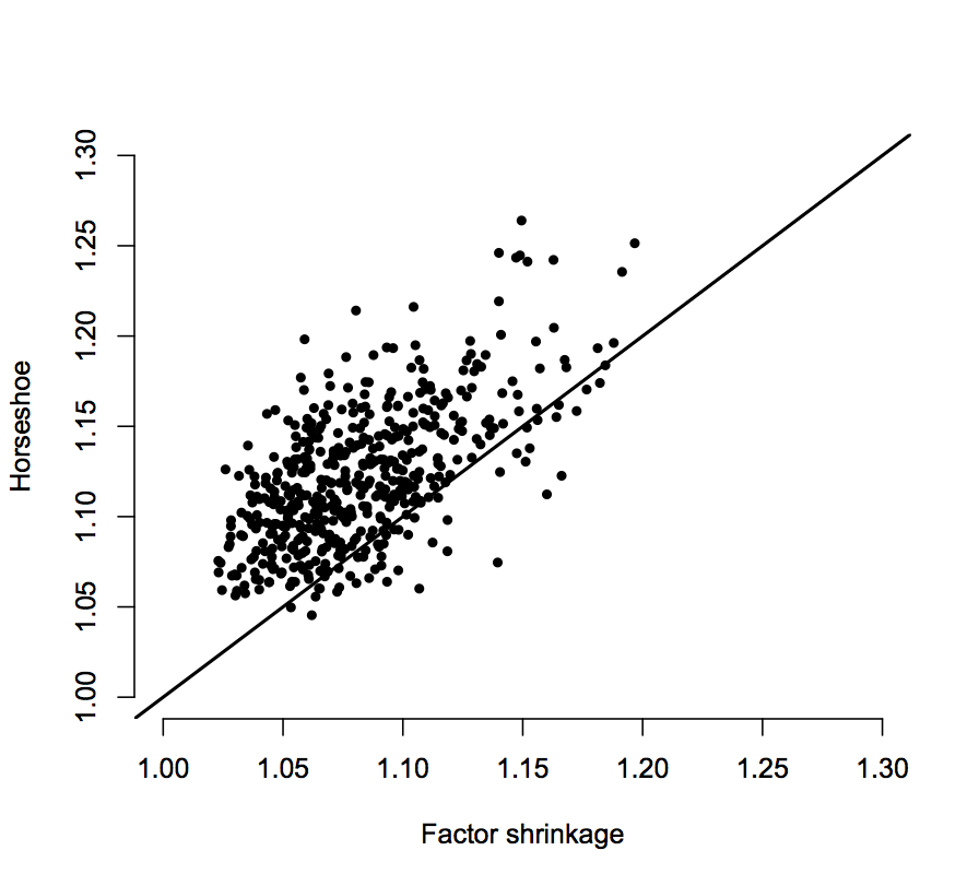
Figure 2. The RMSE as a percentage of the optimal. When factor structure lay beneath idiosyncratic noise, the factor shrinkage prior dominates the unmodified horseshoe prior.

4. An importance resampler for Bayesian IV

Importance sampling a Bayesian IV models proceeds analogously to two-stage least squares in that one first fits a model for $x_{i}\mid\mathrm{z}_{i}$ to obtain estimates of $\boldsymbol{\delta}$. Given $\boldsymbol{\delta}$, estimates for $\beta$, $\alpha$ and $\xi^{2}$ follow straightforwardly from a regression analysis. However, unlike two-stage least squares, which disregards the contribution of $f(x\mid y)$ in forming the first-stage estimate, a Bayesian sampling approach can account for both parts of the likelihood when obtaining posterior draws of $\boldsymbol{\delta}$. Integrating $\alpha,\beta$ and $\xi^{2}$ from the model a priori yields

(25) $$\pi(\boldsymbol{\delta},\sigma_{x}^{2}\mid\mathbf{x},\mathbf{y},\mathbf{Z})\propto\pi(\boldsymbol{\delta},\sigma_{x}^{2}\mid\mathbf{x},\mathbf{Z})f(\mathbf{y}\mid\mathbf{x},\mathbf{Z},\boldsymbol{\delta}),$$

which reveals that one can obtain posterior draws from $\pi(\boldsymbol{\delta},\sigma_{x}^{2}\mid\mathbf{x},\mathbf{y},\mathbf{Z})$ by first sampling from $\pi(\boldsymbol{\delta},\sigma_{x}^{2}\mid\mathbf{x},\mathbf{Z})$ as if $\mathbf{y}$ were not observed, and then resampling with weights proportional to $f(\mathbf{y}\mid\mathbf{x},\mathbf{Z},\boldsymbol{\delta})$. Draws of $(\alpha,\beta,\xi^{2})$ are then obtain compositionally, conditional on a given value of $\boldsymbol{\delta}$.

In the following, assume a normal-inverse-Gamma prior is used for $(\alpha,\beta,\xi^{2})$, with prior mean $\mbox{E}(\alpha)=\mbox{E}(\beta)=0$, covariance of $c\mathbf{I}$, and Gamma shape parameter of $s/2$ and scale parameter of $v/2$. Define $\tilde{x}_{i}\equiv(x_{i},x_{i}-\mathrm{z}_{i}\boldsymbol{\delta})$. Let $\mathbf{M}=c^{-1}\mathbf{I}+\tilde{\mathbf{x}}^{t}\tilde{\mathbf{x}}$, $b=s+\mathbf{y}^{t}\mathbf{y}-\mathbf{y}^{t}\tilde{\mathbf{x}}\mathbf{M}^{-1}\tilde{\mathbf{x}}^{t}\mathbf{y}$, and $a=n+v$. Note that $\tilde{\mathbf{x}}$, $\mathbf{M}$, $a$ and $b$ depend implicitly on $\boldsymbol{\delta}$; in particular, let subscript $j$ denote dependence on the $j$th sample of $\boldsymbol{\delta}$.

1. Draw $N$ samples of $\boldsymbol{\delta}$ from $\pi(\boldsymbol{\delta},\sigma_{x}^{2}\mid\mathbf{x},\mathbf{Z})$ using the sampler described in Carvalho et al. (2009) (though any regression model of choice will suffice here).

2. Resample with weights proportional to $f(\mathbf{y}\mid\boldsymbol{\delta},\mathbf{x},\mathbf{Z})$. Under the conjugate prior described above, $y_{i}\mid z_{i},x_{i},\boldsymbol{\delta},\alpha,\beta,\sigma^{2}_{y\mid x}\sim\mbox{N}(x_{i}\beta+\alpha(x_{i}-\mathrm{z}_{i}^{t}\boldsymbol{\delta}),\sigma^{2}_{y\mid x})$, for each $i$ implies that marginally over $(\alpha,\beta,\sigma^{2}_{y\mid x})$ the $n$-vector of responses has a multivariate $t$-distribution: $\mathbf{y}\mid\mathbf{x},\mathbf{Z},\boldsymbol{\delta}\sim\mbox{t}(a,\mathbf{M})$. Therefore the resampling weights are determined for draw $\boldsymbol{\delta}^{(j)}$ as $w_{j}\propto\mbox{det}(\mathbf{M}_{j})^{-\frac{1}{2}}b_{j}^{-\frac{a_{j}}{2}}$.

3. Finally, sample $(\alpha,\beta,\sigma^{2}_{x})$ given $\boldsymbol{\delta}$ from $\pi(\alpha,\beta,\sigma^{2}_{x},\xi^{2}\mid\mathbf{x},\mathbf{Z},\mathbf{y},\boldsymbol{\delta})$, which is a conjugate Gaussian regression with predictor vector $\tilde{\mathbf{x}}$. More specifically, draw $\sigma^{2}_{x}$ from an inverse-Gamma distribution with shape parameter $b/2$ and scale parameter $a/2$, then draw $(\alpha,\beta)$ as a vector with mean $\mathbf{M}^{-1}\tilde{\mathbf{x}}^{t}\mathbf{y}$ and covariance $\sigma^{2}_{x}\mathbf{M}^{-1}$.

4.1. Synthetic example

This section demonstrates the efficacy of the new approach using synthetic data where the true parameters are known for post-analysis evaluation. The intent of this exercise is not to argue that the factor shrinkage prior is better than alternatives in any absolute sense; the goal is rather to illustrate the role played by predictor-induced bias in posterior inferences in an IV problem.

The parameters of this demonstration are set to mimic the applied analysis in the following section: $\alpha=-0.08$ and $\beta=0.2$. The instruments are generated from a $k=3$ factor model as in the previous simulation. For this demonstration, $p=20$ and $n=60$.

Two priors for the ‘first stage’ regression coefficients $\boldsymbol{\delta}$ are compared, the horseshoe priors and the new factor shrinkage prior. In the instrumental variables regression context mean squared prediction error is not the primary focus, rather it is inferences concerning the structural parameter $\beta$ that are relevant. To reflect this inferential focus, the simulation study considers the coverage and size of the 95% intervals produced by the two models over 250 simulated data sets.

The upshot of the study is that the two regression methods have identical coverage of 94.8% (237 out of 250) that is very nearly identical to the nominal coverage. However, the factor shrinkage prior is, on average, 6% smaller. Figure 3 profiles this difference via a smoothed histogram of this ratio across simulated data sets.

Figure 3. A kernel density plot of the ratio between the posterior 95% interval widths of the horseshoe IV regression versus the factor shrinkage IV regression. The factor shrinkage intervals are smaller on 71% of simulated data sets with an average decrease in interval length of 6%.

5. Empirical study: the elasticity of inter-temporal substitution

Yogo (2004) considers estimating the elasticity of inter-temporal substitution via a linearization of the Euler equation, using macroeconomic data and an instrumental variable analysis. Ng and Bai (2009) extend this analysis by incorporating many additional macro variables (detailed in Ludvigson and Ng (2007)) as instruments and consolidating them into factors using a boosting approach. This section mimics that analysis for comparative purposes, focusing on the 1970:3 to 1998:4 quarterly data for the United States. The complete set of factors use by Ng and Bai (2009) was unobtainable; of their 209 macro-variables a subset of 82 are used here, listed by variable code in the appendix. A representative subset of these macro-variables includes, for example, gross domestic purchases, fixed investment in durable equipment, assets abroad, and net exports.

It is a practically relevant question as to whether or not (lagged) macroeconomic indicators serve as valid instruments in the sense of satisfying the exclusion restriction. On the one hand, under a causal interpretation it seems reasonable to assert that past indicators should only relate to the present economy via the more recent indicators—a sort of Markov property. On the other hand, this narrative falls apart when one considers latent common causes that serve to induce dependence between today’s indicators, yesterdays indicators, and today’s response variable. Such shared common causes clearly violate the desired exclusion restriction. That said, this possibility will not be discussed further here; rather, a narrow comparison is drawn with the results of Ng and Bai (2009), who assume the validity of the macro indicators as instruments.

For reference, the model being fit is as in (6): $f(x,y\mid\mathrm{z})=\mbox{N}_{y\mid x}(x\beta+\alpha(x-\mathrm{z}^{t}\boldsymbol{\delta}),\xi^{2})\mbox{N}_{x}(\mathrm{z}^{t}\boldsymbol{\delta},\sigma_{x}^{2})$, where $y_{i}$ is the quarterly consumption growth (i.e., the change in consumption) in the United States, $x_{i}$ is the real interest rate and $\beta$ denotes the elasticity of inter-temporal substitution (EIS). The instrument vector $\mathrm{z}_{i}$ consists of aforementioned macroeconomic indicators (twice lagged), in addition to the original instruments used inYogo (2004): twice lagged nominal interest rate, inflation, consumption growth, and log dividend-price ratio. See Yogo (2004) section II for a theoretical justification of this model.

One goal of estimating EIS centers around the hypothesis that it is precisely 1, which corresponds to the theoretical proposition that an investor s optimal consumption level is a constant proportion of wealth. If $\beta<1$ is less than 1, the investor s optimal consumption-wealth ratio is increasing in expected returns, if $\beta>1$ it is decreasing.

Additionally, a statistical puzzle was laid out by Yogo concerning testing the hypothesis that EIS is small. One can estimate EIS via two distinct linearizations of the Euler equation. Denote the estimand EIS by $\psi$. One can estimate this directly, as described above, so that $\beta\equiv\psi$. Alternatively, one may interchanging the response variable (consumption growth) and the regressor (real interest rate), whence $\psi\equiv 1/\beta$. When comparing these two approaches, one often finds that both $\psi$ and $1/\psi$ are estimated to be insignificantly different than zero, which gives an apparent contradiction.

To estimate this model, a factor shrinkage prior is placed on $\boldsymbol{\delta}$ and the conjugate normal-inverse-gamma prior described in Section 4 is used for $(\alpha,\beta,\xi^{2})$, with parameters $s=1$, $v=1$, and $c=25$.

Using the direct form of the linearization, so that $\beta\equiv\psi$, the partial factor shrinkage IV model gives a posterior mean rate of inter-temporal substitution of approximately 16%, with 95% credible interval of $(1.4\%,30.8\%)$. This is notably higher than the earlier analyses and the credible interval safely excludes 1. Figures 4 and 5 summarize the posterior inference concerning $\psi\equiv\beta$. Table 3 compares the estimates and standard errors/posterior uncertainty for various estimation methods. Bayesian IV with the factor shrinkage prior is the only approach which gives an estimate of $\beta\equiv\psi$ greater than the OLS estimate (0.16 versus 0.12 respectively); in particular this arises due to a posterior mean estimate of $-0.10$ for $\alpha$.

Using the inverted form of the linearization, so that $\beta\equiv 1/\psi$, the partial factor IV model gives a posterior mean for $\psi$ of 0.41, with 95% credible interval of $(18\%,63\%)$. Although these estimates differ markedly from the direct regression (it is a distinct model with distinct priors), notice that no paradox emerges. In both cases, $\psi$ is estimated to be below 1 and $1/\psi$ is estimated to be above 1. As shown in Figure 6, however, this form of the regression has much weaker signal-to-noise ratio, which results in a multimodal posterior.

Table 3. Estimates of the elasticity of intertemporal substitution using the direct regression ($\beta\equiv\psi$), by various methods: ordinary least squares (OLS), two-stage least squares (TSLS) for Yogo’s original four instruments and for the augmented vector including the 82 macro indicators , Bayesian IV with factor shrinkage prior (FSP), and the boosted factor IV of Ng and Bai (2009), Table 7b ($\mbox{FIV}_{b}$). Standard errors for Bayesian models are given as the posterior standard deviation. All figures are have been rounded to two decimal places for comparison.

Method	$\hat{\psi}\equiv\hat{\beta}$	standard error
OLS	0.12	0.05
TSLS (Yogo)	0.06	0.09
TSLS (full)	0.23	0.10
FSP	0.16	0.08
$\mbox{FIV}_{b}$	0.09	0.06

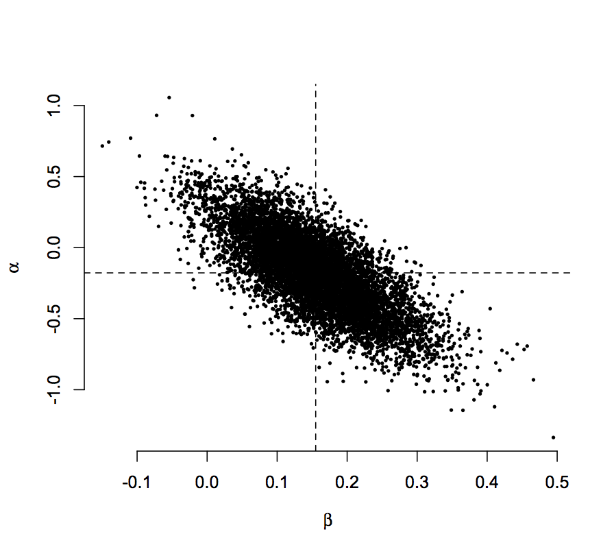
Figure 4. Posterior draws of $(\alpha,\beta)$.

Figure 5. The marginal posterior of the coefficient for elasticity of demand (here $\beta=\psi$). The 90% posterior credible interval does not include 1.

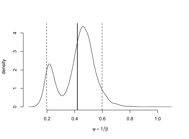
Figure 6. The marginal posterior of the coefficient for elasticity of demand using the inverted regression. The 90% posterior credible interval for $\psi$ still does not include 1. The multimodal posterior is typical of horseshoe-based posteriors in low signal-to-noise ratio problems.

6. Discussion

The factor shrinkage prior leverages an atypical matrix decomposition to create a prior that favors regression coefficients consistent with factor structure underlying the matrix of instruments. In the language of factor analysis, this prior asserts that the treatment variable is more likely to depend on the communalities of the instrument matrix than on the idiosyncrasies. A resampling approach is implemented which allows efficient computation and hence straightforward sensitivity analysis. Specifically, the resampling weights only require computing the determinant of a $d+1$ dimensional matrix, where $d$ is the dimension of the treatment variable (typically one), irrespective of the number of instruments.

Analysis on synthetic data reveals that the new prior performs according to intuition: when factor structure predictive of the treatment is apparent in the matrix of instruments, this concordance with the prior yields tighter inference concerning the treatment effect of interest ($\beta$). Meanwhile, working with a pure regression model sidesteps the least-eigenvalue problem that plagues direct factor modeling. Moreover, the new prior can be used even when the instruments are not jointly Gaussian, such as many binary instruments. More generally, the efficacy of the factor shrinkage prior speaks to the possibilities of combining local shrinkage priors with over-complete dictionaries.

Appendix A Data description

The table below lists the macroeconomic indicators used in our instruments matrix by mnemonic and accompanied by brief abbreviated descriptions. These data came originally from the now-defunct DRI-Global Insight, Basic Economics Database which has been subsumed by the IHS Economics & Country Risk database. Compare to the table in Appendix A.1 in Ludvigson and Ng [2007], of which our list is a subset (some of the series are no longer kept). Following those authors, we apply the following data transformations (DT), indicated by: 1=no transformation; 2 = first difference; 3 = log first difference.

Category/Name	DT	Description
FX
BPAUS	2	U.S. ASSETS ABROAD (NET)
BPB	2	BALANCE ON MERCHANDISE TRADE
GDFXFC	3	CHAIN-TYPE QUANTITY INDEX - EXPORTS OF GOODS AND SERV
GNET	2	NET EXPORTS OF GOODS AND SERV
GRFIW	3	RECEIPT FACTOR INCOME FROM REST OF WORLD
GXIM	1	% CHG FRM PRECEDING PERIOD: IMPORTS
GXMDQF	3	EXPORTS-DURABLE GOODS
GXMNQF	3	EXPORTS-NONDURABLE GOODS
GXMQF	3	EXPORTS-GOODS
GDFMFC	3	CHAIN-TYPE QUANTITY INDEX - IMPORTS OF GOODS AND SERV
Consumption
GDFCDC	3	CHAIN-TYPE QUANTITY INDEX - PCE, DURABLE GOODS
GXDAQF	3	AUTO OUTPUT-EXPORTS
GXPC	1	% CHG FROM PRECEDING PERIOD:PERSONAL CONSUMPTION EXPENDS
GDFCFC	3	CHAIN-TYPE QUANTITY INDEX - PERSONAL CONSUMPTION EXPENDITURES
Prices
GD	3	IMPLICIT PR DEFLATOR: GROSS NATIONAL PRODUCT
GDC	3	IMPLICIT PR DEFLATOR: PERSONAL CONSUMPTION EXPENDITURES
GDCD	3	IMPLICIT PR DEFLATOR: DURABLE GOODS,PCE
GDCN	3	IMPLICIT PR DEFLATOR: NONDURABLE GOODS,PCE
GDCS	3	IMPLICIT PR DEFLATOR: SERVICES, PCE
GDEX	3	IMPLICIT PR DEFLATOR: EXPORTS OF GDS & SERV
GDEXIM	3	TERMS OF TRADE
GDFCC	3	CHAIN-TYPE PRICE INDEX - PERSONAL CONSUMPTION EXPENDITURES
GDFCNC	3	CHAIN-TYPE PRICE INDEX - PCE, NONDURABLE GOODS
GDFCSC	3	CHAIN-TYPE PRICE INDEX - PCE, SERVICES
GDFDCF	3	CHAIN-TYPE PRICE INDEX - NATL DEFENSE EXPENDITURES & GROSS INVESTMENT
GDFDFC	3	CHAIN-TYPE PRICE INDEX - PCE, DURABLE GOODS
GDFDPC	3	CHAIN-TYPE PRICE INDEX- PRODUCERS’ DURABLE EQUIPMENT
GDFEXC	3	CHAIN-TYPE PRICE INDEX - EXPORTS OF GOODS AND SERVICES
GDFGEC	3	CHAIN-TYPE PRICE INDEX - GOVT CONSUMPTION EXPENDITURES & GROSS INV
GDFGFC	3	CHAIN-TYPE PRICE INDEX - FED CONSUMPTION EXPEND & GROSS INVESTMENT
GDFGOC	3	CHAIN-TYPE PRICE INDEX - NONDEF CONS EXPENDITURES & GROSS INVESTMENT
GDFGSC	3	CHAIN-TYPE PRICE INDEX - S&L CONSUMPTION EXPEND & GROSS INVESTMENT
GDFICF	3	CHAIN-TYPE PRICE INDEX - PRIVATE FIXED INVESTMENT
GDFIMC	3	CHAIN-TYPE PRICE INDEX - IMPORTS OF GOODS AND SERV
GDFIRC	3	CHAIN-TYPE PRICE INDEX - RESIDENTIAL
GDFISC	3	CHAIN-TYPE PRICE INDEX - NONRESIDENTIAL STRUCTURES
GDFNRC	3	CHAIN-TYPE PRICE INDEX - NONRESIDENTIAL
GDGF	3	IMPLICIT PR DEFLATOR: FED GOV’T PURCH OF GDS & SERV
GDIS	3	IMPLICIT PR DEFLATOR: PRIVATE NONRESINDENTIAL STRUCTURES
LBGDPU	3	IMPLICIT PRICE DEFLATOR: NONFARM BUSINESS
Fixed Investment
GFINO	3	FIXED INVEST:PRODUCER DURABLE EQUIP
GXIFN	1	% CHG FRM PRECEDING PERIOD:NONRESIDENTIAL FIXED INVESTMENT
GXIFR	1	% CHG FRM PRECEDING PERIOD:RESIDENTIAL FIXED INVESTMENT
GXIPD	1	% CHG FRM PRECEDING PERIOD: NONRESID PRODUCERS’ DUR EQUIP
GXIS	1	% CHG FRM PRECEDING PERIOD: NONRESIDENTIAL STRUCTURES
GXPI	1	% CHG FRM PRECEDING PERIOD:GROSS PRIV DOM INVESTMENT
GDFFIC	3	CHAIN-TYPE QUANTITY INDEX - PRIVATE FIXED INVESTMENT
GDFIFC	3	CHAIN-TYPE QUANTITY INDEX - GROSS PRIVATE DOMESTIC INVESTMENT
Output & Income
GDFDEC	3	CHAIN-TYPE QUANTITY INDEX - NATL DEF EXPENDITURES & GROSS INVESTMENTS
GDFEOC	3	CHAIN-TYPE QUANTITY INDEX - NONDEF CONS EXPEND & GROSS INVESTMENT
GDFFGC	3	CHAIN-TYPE QUANTITY INDEX - FED CONSUMPTION EXPEND & GROSS INVESTMENT
GDFGGC	3	CHAIN-TYPE QUANTITY INDEX - GOVT CONSUMPTION EXPENDITURES & GROSS
GDFGLC	3	CHAIN-TYPE QUANTITY INDEX - S&L CONSUMPTION EXPEND & GROSS INVESTMENT
GDFINC	3	CHAIN-TYPE QUANTITY INDEX - NONRESIDENTIAL
GDFNFC	3	CHAIN-TYPE QUANTITY INDEX - PCE, NONDURABLE GOODS
GDFPDC	3	CHAIN-TYPE QUANTITY INDEX - PRODUCERS’ DURABLE EQUIPMENT
GDFRFC	3	CHAIN-TYPE QUANTITY INDEX - RESIDENTIAL
GDFSFC	3	CHAIN-TYPE QUANTITY INDEX - PCE, SERVICES
GDFSTC	3	CHAIN-TYPE QUANTITY INDEX - NONRESIDENTIAL STRUCTURES
GPY	3	PERSONAL INCOME, TOTAL
GWY	3	NAT’L INCOME: WAGES AND SALARIES
GXNP	1	% CHANGE FROM PRECEDING PERIOD, GNP
GXSAV	3	PERSN’L INCOME: PERS SAVING RATE, GPSAV AS % OF GYD
GXYD	1	% CHG FRM PRECEDING PERIOD: DISP. PERSONAL INCOME
GYDPCQ	3	DISPOSABLE PERSONAL INCOME PER CAPITA IN CHAINED
GYFIR	3	GY BY IND DIV: FINANCE, INSUR AND REAL ESTATE
GYGGE	3	GY BY IND DIV: GOV’T AND GOV’T ENTERPRISES
GYM	3	GY BY IND DIV: MANUFACTURING INDUSTRY
GYMD	3	GY BY IND DIV: DURABLE GOODS MANUFACTURING INDUSTRY
GYMN	3	GY BY IND DIV: NONDURABLE GOODS MANUFACTURING INDUSTRY
GYS	3	GY BY IND DIV: SERVICE INDUSTRIES
GYT	3	GY BY IND DIV: TRANSPORTATION INDUSTRY
GYUT	3	GY BY IND DIV: ELECTRIC, GAS AND SANITARY SEW INDUSTRY
Sales, Orders, Purchases
GXNPD	1	GROSS DOM PURCH
GXNS	1	FINAL SALES OF DOM PROD
GXNSD	1	FINAL SALE TO DOM PURCH
LBOUT	3	OUTPUT PER HOUR ALL PERSONS
LBOUTU	3	OUTPUT PER HOUR ALL PERSONS: NONFARM BUSINESS

References

- Bartholomew and Moustaki [2011] D. Bartholomew and I. Moustaki. Latent Variable models and Factor Analysis: A Unified Approach. Wiley, third edition, 2011.
- Carvalho et al. [2010] C. Carvalho, N. Polson, and J. Scott. The horseshoe estimator for sparse signals. Biometrika, 97:465–480, 2010.
- Carvalho et al. [2009] C. M. Carvalho, N. G. Polson, and J. G. Scott. Handling sparsity via the horseshoe. In International Conference on Artificial Intelligence and Statistics, pages 73–80, 2009.
- Chamberlain and Imbens [1996] G. Chamberlain and G. Imbens. Hierarchical Bayes models with many instrumental variables, 1996.
- Chan and Tobias [2014] J. Chan and J. Tobias. Priors and posterior computation in linear endogenous variable models with imperfect instruments. Journal of Applied Econometrics, 2014.
- Chao and Phillips [1998] J. C. Chao and P. C. Phillips. Posterior distributions in limited information analysis of the simultaneous equations model using the Jeffreys prior. Journal of Econometrics, 87(1):49–86, 1998.
- Clyde et al. [1996] M. Clyde, H. Desimone, and G. Parmigiani. Prediction via orthogonalized model mixing. Journal of the American Statistical Association, 91(435):1197–1208, 1996.
- Conley et al. [2008] T. G. Conley, C. B. Hansen, R. E. McCulloch, and P. E. Rossi. A semi-parametric Bayesian approach to the instrumental variable problem. Journal of Econometrics, 144(1):276–305, 2008.
- Conley et al. [2012] T. G. Conley, C. B. Hansen, and P. E. Rossi. Plausibly exogenous. Review of Economics and Statistics, 94(1):260–272, 2012.
- Cox [1968] D. Cox. Notes on some aspects of regression analysis. Journal of the Royal Statistical Society Series A, 131:265–279, 1968.
- Dreze [1976] J. H. Dreze. Bayesian limited information analysis of the simultaneous equations model. Econometrica: Journal of the Econometric Society, pages 1045–1075, 1976.
- Fazel [2002] M. Fazel. Matrix rank minimization with applications. PhD thesis, Stanford University, 2002.
- Frisch [1934] R. Frisch. Statistical confluence analysis by means of complete regression systems. Technical Report 5, University of Oslo, Economic Institute, 1934.
- Geweke [1996] J. Geweke. Bayesian reduced rank regression in econometrics. Journal of Econometrics, 75(1):121–146, 1996.
- Grant and Boyd [2008] M. Grant and S. Boyd. Graph implementations for nonsmooth convex programs. In V. Blondel, S. Boyd, and H. Kimura, editors, Recent Advances in Learning and Control, Lecture Notes in Control and Information Sciences, pages 95–110. Springer-Verlag Limited, 2008.
- Grant and Boyd [2013] M. Grant and S. Boyd. CVX: Matlab software for disciplined convex programming, version 2.0 beta. http://cvxr.com/cvx, Sept. 2013.
- Griffin and Brown [2012] J. Griffin and P. Brown. Structuring shrinkage: some correlated priors for regression. Biometrika, 99:481–487, 2012.
- Groen and Kapetanios [2009] J. J. Groen and G. Kapetanios. Parsimonious estimation with many instruments. Federal Reserve Bank of New York, Staff Report, (386), 2009.
- Hahn and Hansen [2011] J. Hahn and K. Hansen. Parameter orthogonalization and Bayesian inference with many instruments. Economics Letters, 112(2):207–209, 2011.
- Hahn et al. [2013] P. Hahn, C. M. Carvalho, and S. Mukherjee. Partial factor modeling: predictor-dependent shrinkage for linear regression. Journal of the American Statistical Association, 108(503):999–1008, 2013.
- Jolliffe [1982] I. T. Jolliffe. A note on the use of principal components in regression. Journal of the Royal Statistical Society, Series C, 31(3):300–303, 1982.
- Kapetanios and Marcellino [2010] G. Kapetanios and M. Marcellino. Factor-GMM estimation with large sets of possibly weak instruments. Computational Statistics & Data Analysis, 54(11):2655–2675, 2010.
- Kleibergen and Zivot [2003] F. Kleibergen and E. Zivot. Bayesian and classical approaches to instrumental variable regression. Journal of Econometrics, 114(1):29–72, 2003.
- Liang et al. [2007] F. Liang, S. Mukherjee, and M. West. The use of unlabeled data in predictive modeling. Statistical Science, 22(2):189–205, 2007.
- Liang et al. [2008] F. Liang, R. Paulo, G. Molina, M. Clyde, and J. Berger. Mixtures of g priors for Bayesian variable selection. Journal of the American Statistical Association, 103:410–423, 2008.
- Lindley and El-Sayed [1968] D. Lindley and G. El-Sayed. The Bayesian estimation of a linear functional relationship. Journal of the Royal Statistical Society. Series B, 30:190–202, 1968.
- Lopes and Polson [2014] H. F. Lopes and N. G. Polson. Bayesian instrumental variables: priors and likelihoods. Econometric Reviews, 33(1-4):100–121, 2014.
- Lopes et al. [2008] H. F. Lopes, E. Salazar, and D. Gamerman. Spatial dynamic factor analysis. Bayesian Analysis, 3(4):759–792, 2008.
- Ludvigson and Ng [2007] S. C. Ludvigson and S. Ng. The empirical risk–return relation: A factor analysis approach. Journal of Financial Economics, 83(1):171–222, 2007.
- Maruyama and George [2011] Y. Maruyama and E. I. George. Fully Bayes factors with a generalized g-prior. The Annals of Statistics, 39(5):2740–2765, 2011.
- Murray et al. [2013] J. S. Murray, D. B. Dunson, L. Carin, and J. E. Lucas. Bayesian Gaussian copula factor models for mixed data. Journal of the American Statistical Association, 108(502):656–665, 2013.
- Ng and Bai [2009] S. Ng and J. Bai. Selecting instrumental variables in a data rich environment. Journal of Time Series Econometrics, 1(1), 2009.
- Ning et al. [2013] L. Ning, T. T. Georgiou, A. Tannenbaum, and S. P. Boyd. Linear models based on noisy data and the Frisch scheme. arXiv preprint arXiv:1304.3877, 2013.
- Polson and Scott [2012] N. Polson and J. Scott. Local shrinkage rules, Levy processes and regularized regression. Journal of the Royal Statistical Society, B, 74(2):287–311, 2012.
- Rossi et al. [2006] P. E. Rossi, G. M. Allenby, and R. McCulloch. Bayesian statistics and marketing. Series in Probability and Statistics. Wiley, 2006.
- Shapiro [1982] A. Shapiro. Weighted minimum trace factor analysis. Psychometrika, 47(3):243–264, 1982.
- Spearman [1904] C. Spearman. General intelligence, objectively determined and measured. American Journal of Psychology, 15:201–293, 1904.
- West [2003] M. West. Bayesian factor regression models in the “large p, small n” paradigm. In J. M. Bernardo, M. Bayarri, J. Berger, A. Dawid, D. Heckerman, A. Smith, and M. West, editors, Bayesian Statistics 7, pages 723–732. Oxford University Press, 2003.
- Yogo [2004] M. Yogo. Estimating the elasticity of intertemporal substitution when instruments are weak. Review of Economics and Statistics, 86(3):797–810, 2004.
- Zellner [1986] A. Zellner. On assessing prior distributions and Bayesian regression analysis with g-prior distributions. In Bayesian Inference and Decision Techniques: Essays in Honor of Bruno de Finetti, pages 233–243. Amsterdam: North-Holland, 1986.