Tidal radii and destruction rates of globular clusters in the Milky Way due to bulge-bar and disk shocking

Abstract

We calculate orbits, tidal radii, and bulge-bar and disk shocking destruction rates for 63 globular clusters in our Galaxy. Orbits are integrated in both an axisymmetric and a non-axisymmetric Galactic potential that includes a bar and a 3D model for the spiral arms. With the use of a Monte Carlo scheme, we consider in our simulations observational uncertainties in the kinematical data of the clusters. In the analysis of destruction rates due to the bulge-bar, we consider the rigorous treatment of using the real Galactic cluster orbit, instead of the usual linear trajectory employed in previous studies. We compare results in both treatments. We find that the theoretical tidal radius computed in the non-axisymmetric Galactic potential compares better with the observed tidal radius than that obtained in the axisymmetric potential. In both Galactic potentials, bulge-shocking destruction rates computed with a linear trajectory of a cluster at its perigalacticons give a good approximation to the result obtained with the real trajectory of the cluster. Bulge-shocking destruction rates for clusters with perigalacticons in the inner Galactic region are $smaller$ in the non-axisymmetric potential, as compared with those in the axisymmetric potential. For the majority of clusters with high orbital eccentricities ($e>0.5$), their total bulge+disk destruction rates are $smaller$ in the non-axisymmetric potential.

1 Introduction

In two previous papers (Allen et al., 2006, 2008, hereafter Papers I and II) tidal radii and destruction rates due to bulge and disk shocking were computed for 54 globular clusters in our Galaxy, using axisymmetric and non-axisymmetric Galactic potentials. In Paper I the non-axisymmetric Galactic potential included the Galactic bar, and in Paper II the additional effect of three dimensional (3D) spiral arms was also analyzed. The models for these non-axisymmetric components given by Pichardo et al. (2003, 2004) were employed in those computations. The absolute proper motion data needed to compute the Galactic orbits of the globular clusters were obtained from the extensive studies of Dinescu et al. (1997, 1999a, 1999b, 2000, 2001, 2003) and Casetti-Dinescu et al. (2007), who have computed the proper motions for a good fraction of the total number of globular clusters; for other clusters, Dinescu et al. (1999b) have compiled the proper motion data from various sources. Lately, Casetti-Dinescu et al. (2010) have given the absolute proper motions of other nine globular clusters, and Casetti-Dinescu et al. (2013) present new absolute proper motions of NGC 6397, NGC 6626, and NGC 6656; thus now we dispose of absolute proper motion data for a total of 63 globular clusters in our Galaxy.

For the new sample of 63 globular clusters, we compute again their tidal radii and destruction rates due to bulge and disk shocking, now with some improvements. We use axisymmetric and non-axisymmetric Galactic potentials, the later including both the spiral arms and the Galactic bar models of Pichardo et al. (2003, 2004), as in Paper II. A first part of our improvements has to do with this Galactic potential, the initial orbital conditions of the globular clusters, and the uncertainties in the computed quantities: (a) the Galactic potential is now rescaled to recent values of the galactocentric distance and rotation velocity of the local standard of rest, as found by Brunthaler et al. (2011), (b) we use the solar velocity obtained by Schönrich et al. (2010), (c) the late compilation of clusters properties given by Harris (2010) is used to update other parameters employed in our computations, and (d) we make Monte Carlo simulations to estimate the uncertainties in the tidal radii and destruction rates, and compare with estimates in Papers I and II.

The second part of our improvements refers to the procedure to compute destruction rates. In Papers I, II and in previous studies of tidal heating due to the interaction with the Galactic bulge and heating by disk shocking (e.g., Aguilar et al., 1988; Gnedin & Ostriker, 1997, 1999), the impulse approximation and a straight-path cluster trajectory have been employed. Here we relax the straight-path approximation and follow the more rigorous treatment given by Gnedin et al. (1999a), who employ a fit to the tidal acceleration along the true Galactic orbit of the cluster. In this paper this procedure is undertaken in our non-spherical Galactic potentials, as opposed to the spherical potential used by Gnedin et al. (1999a). The results are compared with those obtained using the usual straight-path aproximation.

In $\S$ 2 we give the globular cluster data employed in our study. The Galactic potential and its parameters are presented in $\S$ 3. In $\S$ 4 some properties of the Galactic orbits in both the axisymmetric and non-axisymmetric potentials are tabulated, and for some clusters we show their meridional orbits. The tidal radii are analyzed in $\S$ 5. The needed formulism of destruction rates using the real trajectories of globular clusters is summarized in $\S$ 6, and our results are presented in $\S$ 8. In $\S$ 9 we present our conclusions.

2 Employed data for the globular clusters

In Table 1 we list the cluster parameters employed in our study. Equatorial coordinates $(\alpha,\delta)$, are given in columns 2 and 3. The distance $r$ and radial velocity $v_{r}$, in columns 4 and 5, are taken from the recent compilation by Harris (2010). The absolute proper motions, ${\mu}_{x}$ = ${\mu}_{\alpha}\cos{\delta}$, ${\mu}_{y}$ = ${\mu}_{\delta}$, in columns 6 and 7, are the values given by Dinescu et al. (1997, 1999a, 1999b, 2000, 2001, 2003) and Casetti-Dinescu et al. (2007, 2010, 2013), except for 47 Tuc (NGC 104) and M4 (NGC 6121) whose values are taken from Anderson & King (2003) and Bedin et al. (2003), respectively. As in Papers I and II, the mass of a cluster, $M_{c}$, given in column 8, is computed using a mass-to-light ratio $(M/L)_{V}$ = 2 $M_{\odot}/L_{\odot}$. In $\S$ 5 we also employ for some clusters their $M_{c}$ computed with dynamical mass-to-light ratios given by McLaughlin & van der Marel (2005) . The observed tidal radius $r_{td}$ (we call $r_{td}$=$r_{K}$ if this radius is computed with a King model (King, 1962)) is not listed by Harris (2010), but as he points out, it can be computed with his listed values for the concentration, $c$, and core radius, $r_{c}$, only for those clusters with a non-collapsed core. For clusters with a collapsed core, Harris suggests to take $r_{td}$ estimated by McLaughlin & van der Marel (2005) and Peterson & King (1975). For this type of clusters, and listed in Table 1, McLaughlin & van der Marel (2005) give $r_{td}$ for NGC 362, NGC 1904, NGC 6266, and NGC 6723; we take their $r_{td}$ for a King model, which is the model we use in our computations. For other clusters in Table 1, Peterson & King (1975) estimate $r_{td}$ in NGC 6397, NGC 6752, NGC 7078, and NGC 7099. These values of $r_{td}$ from McLaughlin & van der Marel (2005) and Peterson & King (1975) are transformed according to the distances $r$ given by Harris (2010). For NGC 6284, NGC 6293, NGC 6342, and NGC 6522, we take $r_{td}$ from Harris’ previous compilation, transformed with his new listed distances. Column 9 gives the final $r_{td}$=$r_{K}$ employed values, and column 10 the half-mass radius, $r_{h}$, in each cluster.

3 The Galactic potential

In our analysis we employ axisymmetric and non-axisymmetric models for the Galactic gravitational potential. The axisymmetric model is based on the Galactic model of Allen & Santillán (1991), which gives a circular rotation speed on the Galactic plane ${\Theta}_{0}$ $\approx$ 220 km/s at its assumed Sun’s Galactocentric distance $R_{0}$ = 8.5 kpc. This model is scaled to the new Galactic parameters ${\Theta}_{0}$, $R_{0}$ given by Brunthaler et al. (2011): ${\Theta}_{0}$ = 239$\pm$7 km/s, $R_{0}$ = 8.3$\pm$0.23 kpc.

The non-axisymmetric Galactic model is built from the scaled axisymmetric model. First, all the mass in the spherical bulge component in this axisymmetric model is employed to built the Galactic bar. In Papers I and II, where only 70$\%$ of the bulge mass was employed to built the bar, we have mentioned some properties of the model used for this bar component. We use the third bar model given by Pichardo et al. (2004) (the model of superposition of ellipsoids), which approximates the boxy COBE/DIRBE brightness profiles shown by Freudenreich (1998).

We also consider a 3D gravitational potential to represent the spiral arms. The model used for these arms, called PERLAS, is given by Pichardo et al. (2003), and has already been employed in Paper II. The total mass of the 3D spiral arms is taken as a small fraction of the mass in the disk component of the scaled axisymmetric model. We take $M_{\rm arms}/M_{\rm disk}$ = 0.04$\pm$0.01, considered by Pichardo et al. (2012) in their analysis of the maximum value on the Galactic plane of the parameter $Q_{T}$ (Sanders & Tubbs, 1980; Combes & Sanders, 1981), which, as a function of Galactocentric distance, is the ratio of the maximum azimuthal force of the spiral arms to the radial axisymmetric force at a given distance.

The mass density at the center of the spiral arms falls exponentially with Galactocentric distance, and we take its corresponding radial scale length equal to the one of the Galactic exponential disk modeled by Benjamin et al. (2005): $H$ = 3.9$\pm$0.6 kpc, using $R_{0}$ = 8.5 kpc, scaled now with the new value of $R_{0}$.

Other properties of the Galactic bar and the Galactic spiral arms, have been collected in Pichardo et al. (2012). We use the following parameters in our computations: a) the present angle between the bar’s major axis and the Sun-Galactic center line is taken as 20^∘, b) the angular velocity of the bar is in the range $\approx$ 55$\pm$5 ${\rm\,km\,s^{-1}{kpc}^{-1}}$, c) we consider the pitch angle of the spiral arms in the range $\approx$ 15.5$\pm$3.5^∘, d) the range for the angular velocity of the spiral arms is $\approx$ 24$\pm$6 ${\rm\,km\,s^{-1}{kpc}^{-1}}$.

Table Tidal radii and destruction rates of globular clusters in the Milky Way due to bulge-bar and disk shocking summarizes all the parameters employed in our Galactic models, along with the Solar velocity $(U,V,W)_{\odot}$ obtained by Schönrich et al. (2010) (here $U$ is taken negative towards the Galactic center) and its uncertainties estimated by Brunthaler et al. (2011).

4 Properties of the Galactic orbits

For the computation of the Galactic orbits we have employed the Bulirsch-Stoer algorithm given by Press et al. (1992), and also the Runge-Kutta algorithm of seventh-eight order elaborated by Fehlberg (1968). In our problem both algorithms give practically the same results, and due to the complicated mathematical forms of the gravitational potentials of the non-axisymmetric Galactic components (bar and 3D spiral arms), we have favored the Runge-Kutta algorithm to reduce the computing time, specially in the Monte Carlo calculations. The Bulirsch-Stoer algorithm is employed mainly in the computations with the axisymmetric potential.

In Table 3 we give for each cluster some orbital parameters obtained with the non-axisymmetric (first line) and axisymmetric (second line) potentials. Except for the data given in columns 8 and 9, whose associated time interval is commented in the next section, the data presented in this table correspond to a backward time integration of 5 $\times$ $10^{9}$ yr in the axisymmetric case, and from $10^{9}$ to 3 $\times$ $10^{9}$ yr in the non-axisymmetric case, depending on the cluster. The second, third, and fourth columns show the average perigalactic distance, the average apogalactic distance, and the average maximum distance from the Galactic plane, respectively. The fifth column gives the average orbital eccentricity, this eccentricity defined as $e=(r_{max}-r_{min})/(r_{max}+r_{min})$, with $r_{min}$ and $r_{max}$ successive perigalactic and apogalactic distances. Columns 6 and 7 give the orbital energy per unit mass, $E$, and the z-component of angular momentum per unit mass, $h$, only in the axisymmetric potential, where these two quantities are constants of motion. Columns 8 and 9 list tidal radii, which are discussed in the next section.

In Figures 1 and 2 we show meridional orbits for some clusters, whose NGC number is given. In each pair of columns the orbit in the axisymmetric potential is shown in the left frame, and that in the non-axisymmetric potential in the right frame. We choose this sample of clusters to illustrate how strong the effect of the non-axisymmetric Galactic components can be. The most conspicuous difference between the computations in both potentials is the orbital radial extent. This has important consequences in the clusters tidal radii, as shown in the next section.

Figures 3, 4, and 5 show the comparison in both Galactic potentials of the average perigalactic distance, average apogalactic distance, and average maximum distance from the Galactic plane, given respectively in the second, third, and fourth columns of Table 3. Values in the axisymmetric potential (with a subindex ’ax’) and non-axisymmetric potential (with a subindex ’nax’) are given in the horizontal and vertical axes, respectively. The uncertainties shown in these figures are estimated with the differences from corresponding quantities obtained in the minimum and maximum energy orbits in each cluster, according to the uncertainties in the cluster radial velocity, distance, and proper motions.

5 Tidal radii

5.1 Comparison of theoretical and observed tidal radii in the axisymmetric and non-axisymmetric Galactic potentials

5.1.1 Comparison with observed King tidal radii $r_{K}$

As in Papers I and II, for each globular cluster, and in both axisymmetric and non-axisymmetric Galactic potentials employed in our analysis, we compute a theoretical tidal radius using two expressions. The first is King’s formula (King, 1962)

$$r_{K_{t}}=\left[\frac{M_{c}}{M_{g}(3+e)}\right]^{1/3}r_{min},$$ (1)

where $M_{c}$ is the mass of the cluster, $M_{g}$ is an effective galactic mass, $e$ is the orbital eccentricity as defined in the previous section, and $r_{min}$ is the perigalactic distance. The mass $M_{g}$ is taken as the equivalent central mass point which gives an acceleration at the given perigalactic position with a magnitude equal to the magnitude of the actual acceleration at this point in the corresponding Galactic potential.

The second expression is the one proposed in Paper I, computed at the perigalactic position

$$r_{\ast}=\left[\frac{GM_{c}}{\left(\frac{\partial F_{x^{\prime}}}{\partial x^{\prime}}\right)_{{\bf r^{\prime}}=0}+\dot{\theta}^{2}+\dot{\varphi}^{2}\sin^{2}{\theta}}\right]^{1/3},$$ (2)

with $F_{x^{\prime}}$ the component of the Galactic acceleration along the line $x^{\prime}$ joining the cluster with the Galactic center, and its partial drivative evaluated at the given perigalactic point. The angles ${\varphi}$ and ${\theta}$ are angular spherical coordinates of the cluster in an inertial galactic frame.

In Paper I these two expressions for a theoretical tidal radius gave similar values. For a given Galactic potential, this result is maintained in the present computations. Columns 8 and 9 in Table 3 give the average values $<$$r_{K_{t}}$$>$, $<$$r_{\ast}$$>$ of $r_{K_{t}}$ and $r_{\ast}$, over the last $10^{9}$ yr (in some clusters this time interval is extended to have a few perigalactic points).

In this and next sections of $\S$ 5 we make some comparisons using $r_{K_{t}}$ given by Eq. (1). The first comparison is $r_{K_{t}}$ with the observed tidal radius (also called the limiting radius) $r_{td}$=$r_{K}$ listed in Table 1, estimated with a King model (King, 1962). In Figures 6 and 7 we show with big filled squares this comparison in the axisymmetric and non-axisymmetric Galactic potentials. These points have two marks: clusters in which the tidal radius $<$$r_{K_{t}}$$>$ computed with the non-axisymmetric potential is greater than $<$$r_{K_{t}}$$>$ computed with the axisymmetric potential, are marked with encircled points; crossed points correspond to clusters in which $<$$r_{K_{t}}$$>$ computed with the non-axisymmetric potential is less than $<$$r_{K_{t}}$$>$ computed with the axisymmetric potential. These marks are shown in both figures. Thus, encircled and crossed points in Figure 6 will move upwards and downwards, respectively, to give the corresponding Figure 7. As in Papers I and II, the uncertainty in $<$$r_{K_{t}}$$>$, or $<$$r_{\ast}$$>$, is estimated in each cluster by computing $<$$r_{K_{t}}$$>$ in the minimum and maximum energy orbits, according to the uncertainties in the cluster radial velocity, distance, and proper motions. The small empty squares and empty triangles in Figures 6 and 7 show the values of $<$$r_{K_{t}}$$>$ in these minimum and maximum energy orbits, respectively.

From these figures we note that $<$$r_{K_{t}}$$>$ computed in the non-axisymmetric potential compares better with $r_{K}$: many clusters whose points lie below the line of coincidence in Figure 6, are closer to this line in Figure 7; these are the encircled points. Likewise, several clusters with points (now the crossed points) above the line of coincidence in Figure 6, are closer to this line in Figure 7. The rearrangement of the encircled points is the most conspicuous.

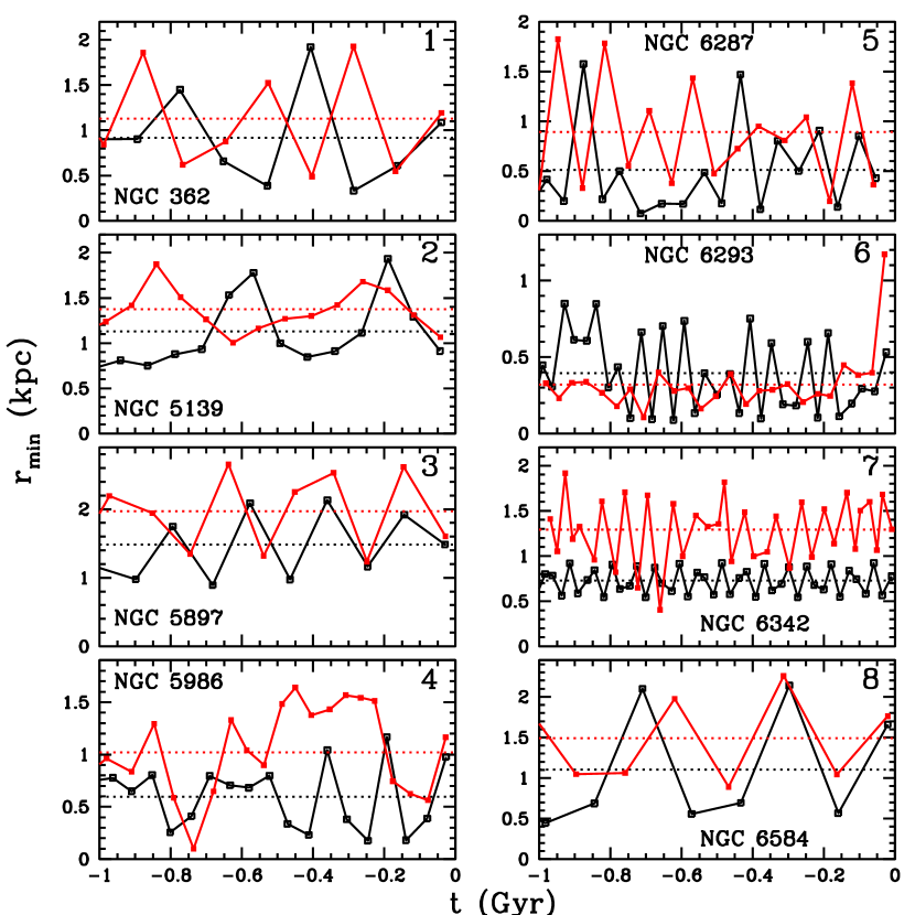
Figure 8: Perigalactic distance as a function of time over the last $10^{9}$ yr for the sample of globular clusters with numbered encircled points in Figure 6. Black dots joined with black lines show the values in the axisymmetric potential; those in red correspond to the non-axisymmetric potential. The horizontal dotted lines show the corresponding average values. In each frame the cluster name and its identification number in Figure 6 are given.

In Figure 6 a sample of eight clusters has been selected, represented by encircled points numbered from 1 to 8, and correspond to NGC 362, NGC 5139, NGC 5897, NGC 5986, NGC 6287, NGC 6293, NGC 6342, and NGC 6584, respectively. For these clusters, in Figure 8 we give the values of their perigalactic distance, $r_{min}$, as a function of time, over the last $10^{9}$ yr; black dots joined by black lines show the values in the axisymmetric potential, and the dots and lines in red correspond to the non-axisymmetric potential. The black and red horizontal dotted lines show the corresponding average value of $r_{min}$ in the given interval of time. Each frame shows the cluster name and also the identification number in Figure 6. Except for NGC 6293, Figure 8 partly explains why in the case of encircled points, $<$$r_{K_{t}}$$>$ increases using the non-axisymmetric potential: in these clusters, the average value of $r_{min}$ obtained with the non-axisymmetric potential (red horizontal dotted lines) is greater than the corresponding average in the axisymmetric potential (black horizontal dotted lines).

The other factor which helps to understand the rearrangement of encircled points from Figure 6 to Figure 7 (at least those in the considered sample) is the value of the effective galactic mass $M_{g}$ employed in King’s formula Eq. (1). As stated in $\S$ 3, the original concentrated spherical bulge in the axisymmetric potential was employed to built the bar; thus, due to the less mass concentration of the non-axisymmetric potential in the inner Galactic region (see upper frame in figure 7 in Paper I), the contribution of the bar to $M_{g}$ computed at a given perigalactic distance in this inner region is expected to decrease compared with the contribution of the spherical bulge in the axisymmetric potential. In general, the value of $M_{g}$ in the non-axisymmetric potential will depend on the position of the perigalactic point relative to the axes of the Galactic bar, because this bar generates a non-axisymmetric force field. In addition, $M_{g}$ has also the effect of the spiral arms with their relative orientation to the axes of the bar at the time of occurrence of the perigalactic point. Thus, the value of $M_{g}$ depends on the specific perigalactic point.

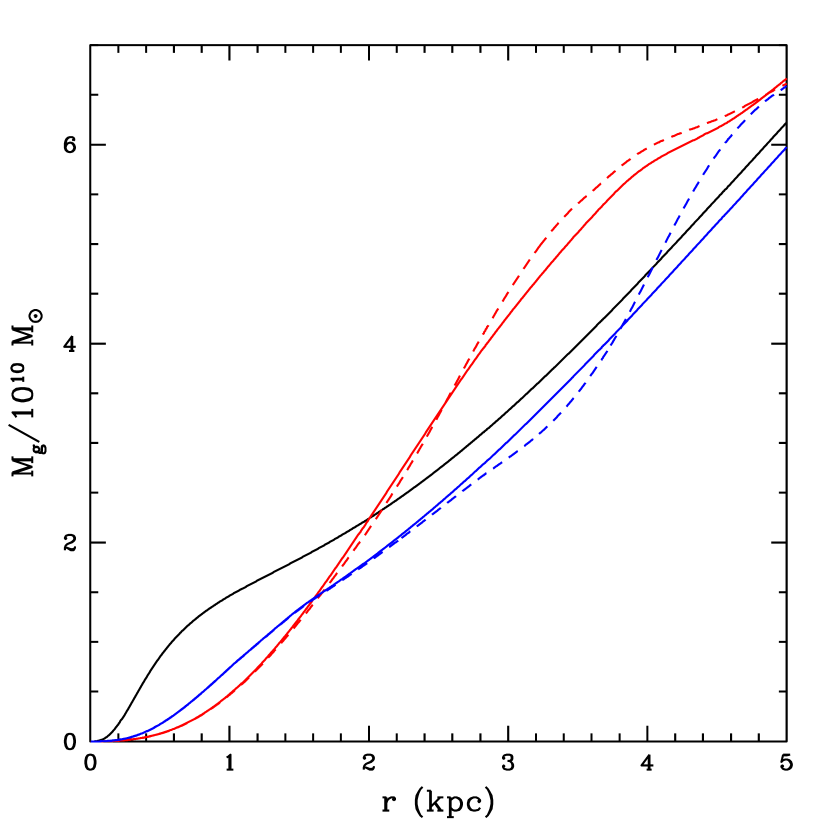
Figure 9: $M_{g}$ computed on the Galactic plane as a function of distance to the Galactic center. Values in the axisymmetric potential are shown with the black line; the continuous and dashed red and blue lines show values in the non-axisymmetric potential, along the major (red) and minor (blue) axes of the bar. The continuous red and blue lines show the contribution of the axisymmetric background and Galactic bar in this potential, and the corresponding dashed lines includes the spiral arms with a particular orientation (see main text).

To illustrate these comments, in Figure 9 we give values of $M_{g}$ computed on the Galactic plane as a function of distance to the Galactic center. The black line corresponds to the axisymmetric potential; the continuous red and blue lines show values of $M_{g}$ due to the axisymmetric background (i.e. disk and spherical dark halo) plus the Galactic bar, along the major and minor axes of the bar, respectively. The dashed red and blue lines show values of $M_{g}$ along these major and minor axes with the addition of the spiral arms, i.e. considering all the mass components in the non-axisymmetric potential, taking in particular the major axis of the bar as the line where the spiral arms originate in the inner Galactic region. Thus, note the smaller values that $M_{g}$ can take in the inner Galactic region in the non-axisymmetric potential.

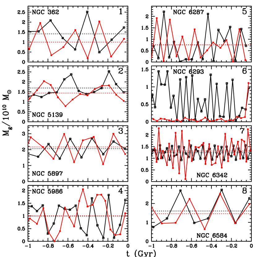
Figure 10: Effective galactic mass $M_{g}$ employed in Eq. (1) as a function of time over the last $10^{9}$ yr for the clusters in Figure 8. The correspondence of colors is the same as in Figure 8. The horizontal dotted lines (not plotted in NGC 6293) show the average values of $M_{g}$.

Figure 10 shows the values of $M_{g}$ at the perigalactic points in Figure 8. The correspondence of colors in this figure is that given in Figure 8. The horizontal dotted lines show the average values of $M_{g}$ over the last $10^{9}$ yr; these lines are not plotted in NGC 6293 to avoid confusion in the lower continuous red line. The average values of $M_{g}$ in the axisymmetric and non-axisymmetric potentials almost coincide in the clusters NGC 5897, NGC 5986, NGC 6287, NGC 6342, and NGC 6584; thus in these clusters the increase of the average value of $r_{min}$ in the non-axisymmetric potential explains the corresponding increase of $<$$r_{K_{t}}$$>$. For the remaining clusters in this sample, NGC 362, NGC 5139, and NGC 6293, the average value of $M_{g}$ is sensibly smaller in the non-axisymmetric potential, specially in NGC 6293. This result combined with the increase of $r_{min}$, gives a net increase of $<$$r_{K_{t}}$$>$ for NGC 362 and NGC 5139 in the non-axisymmetric potential. On the other hand, in NGC 6293 the strong decrease of the average value of $M_{g}$ in the non-axisymmetric potential compared with that in the axisymmetric potential, counteracts the corresponding slight decrease of the average value of $r_{min}$ shown in Figure 8, giving a net increase of $<$$r_{K_{t}}$$>$ in the non-axisymmetric potential.

5.1.2 Comparison with improved observed limiting radii

Recently Miocchi et al. (2013) have derived the radial stellar density profiles of 26 Galactic globular clusters from resolved star counts, using high-resolution $HubbleSpaceTelescope$ observations. In particular, they derive the limiting radius $r_{l}$, what we call the observed tidal radius, employing King and Wilson (Wilson, 1975) models. Considering the clusters in common between our sample and their 26 clusters, we have taken their best fits given by the least value of the reduced ${\chi}^{2}$ in the third column of their table 2, and compare our theoretical tidal radii $r_{K_{t}}$ with their corresponding limiting radii $r_{l}$.

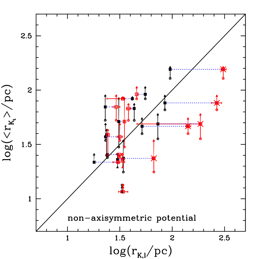
Figure 11: Red points: comparison between $r_{K_{t}}$ and the limiting radius $r_{l}$ obtained by Miocchi et al. (2013) for some clusters in our sample. The comparison is made in the non-axisymmetric potential. Black points are corresponding points from $r_{K_{t}}$ vs $r_{K}$ in Figure 7. Horizontal displacements between red and black points are shown with dotted blue lines. Red crossed points correspond to clusters in which a Wilson model gives the best fit.

We give this comparison in Figure 11, in particular in the non-axisymmetric potential. The black points with their uncertainties are points already plotted in Figure 7 with corresponding King tidal radii $r_{K}$ employed in that figure. The red points are the comparison between $r_{K_{t}}$ with $r_{l}$; the uncertainties in $r_{l}$ are computed with data in table 2 of Miocchi et al. (2013) using distances given in our Table 1. Thus these points are displaced in the horizontal axis with respect to the black points. The displacements are shown with dotted blue lines. Red crossed points correspond to clusters in which a Wilson model gives the best fit to the density profile. The comparison between $r_{K_{t}}$ with $r_{l}$ is almost the same as $r_{K_{t}}$ vs $r_{K}$ in Figure 7, except for the five red crossed points, where $r_{l}$ is about a factor of 2-3 greater than $r_{K}$ and $r_{K_{t}}$. These five points correspond to NGC 288, NGC 5024 (M53), NGC 5272 (M3), NGC 5466, and NGC 5904 (M5). As commented in Paper I, the last three clusters appear to be dissolving (Leon et al., 2000; Odenkirchen & Grebel, 2004; Belokurov et al., 2006); also, NGC 288 has extended tails (Grillmair et al., 2004), and NGC 5024 is possibly an accreted cluster (Mackey & Gilmore, 2004). Thus in these five clusters $r_{l}$ will be an upper bound for the tidal radius; some stars contributing to $r_{l}$ may be already escaping from the cluster.

5.1.3 Comparison with improved cluster masses

In their study of structural properties of massive star clusters, McLaughlin & van der Marel (2005) have obtained dynamical mass-to-light ratios $(M/L)_{V}$ for 57 Galactic globular clusters. In this part we compute $r_{K_{t}}$ for clusters in common between our sample and those listed in their table 13, now with the cluster mass $M_{c}$ computed with their $(M/L)_{V}$, instead of $(M/L)_{V}$ = 2 $M_{\odot}/L_{\odot}$ employed in our study. With these new values of $r_{K_{t}}$, we compare $r_{K_{t}}$ vs $r_{K}$ in the non-axisymmetric potential.

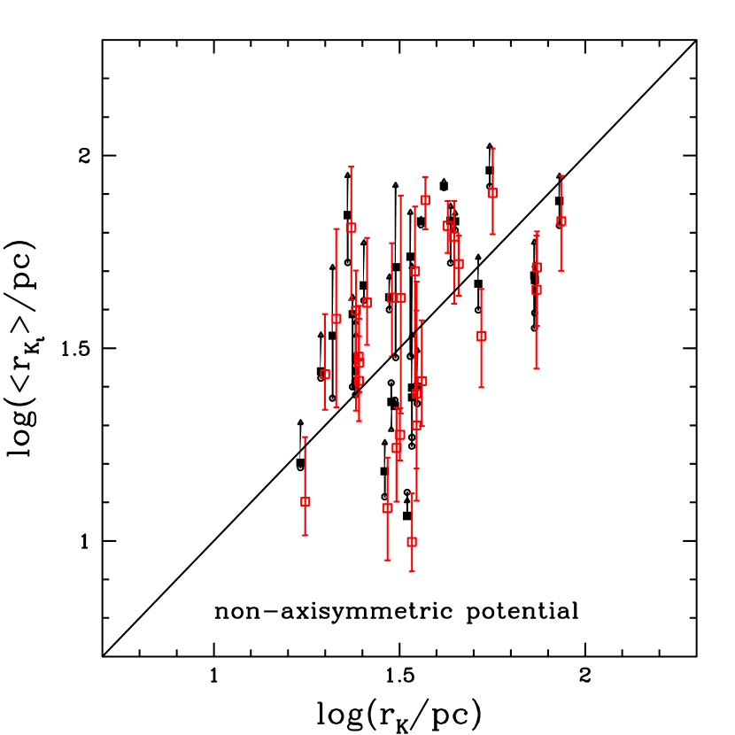
Figure 12: Red points: comparison of $r_{K_{t}}$ vs $r_{K}$ in the non-axisymmetric potential computing the cluster mass $M_{c}$ with dynamical mass-to-light ratios given by McLaughlin & van der Marel (2005). Black points: corresponding points from Figure 7 using $(M/L)_{V}$ = 2 $M_{\odot}/L_{\odot}$. For clarity, the red points are slightly displaced to the right of the black points.

Figure 12 shows this comparison. The black points are points from Figure 7, using $(M/L)_{V}$ = 2 $M_{\odot}/L_{\odot}$; the red points employ the $(M/L)_{V}$ values of McLaughlin & van der Marel (2005) with their uncertainties. For clarity in the figure, these red points are slightly displaced to the right of the black points. Thus, there is no much difference with respect to the comparison made in Figure 7, and the standard $(M/L)_{V}$ = 2 $M_{\odot}/L_{\odot}$ is a convenient test in our analysis.

5.2 Tidal radii with Monte Carlo computations

The comparison of theoretical and observed tidal radii made in the last section was repeated, now using Monte Carlo simulations. The uncertainties in the cluster distance, radial velocity, and proper motions, listed in Table 1, plus the uncertainties of the Galactic parameters listed in Table Tidal radii and destruction rates of globular clusters in the Milky Way due to bulge-bar and disk shocking, were considered as 1$\sigma$ variations in a Gaussian Monte Carlo sampling. For each cluster we computed a few hundreds of orbits. In each sampled cluster orbit computed backward in time, we found the average $<$$r_{K_{t}}$$>$ over the last $10^{9}$ yr, and in turn, with all these values in a given cluster, determined its corresponding global average, denoted by $\langle r_{K_{t}}\rangle$, and its 1$\sigma$ variation.

Figures 13 and 14 show the comparison of $\langle r_{K_{t}}\rangle$ with $r_{K}$ in the axisymmetric and non-axisymmetric Galactic potentials. The error bars in both figures correspond to the computed 1$\sigma$ variation. With these Monte Carlo calculations we obtain nearly the same comparisons shown in Figures 6 and 7; thus, again our conclusion is that $\langle r_{K_{t}}\rangle$ compares better with $r_{K}$ employing the non-axisymmetric potential. These Figures 13 and 14 also show that the estimate of the uncertainty in $<$$r_{K_{t}}$$>$ done in $\S$ 5.1 using the minimum and maximum energy orbits, is acceptable.

An additional plotted point in Figures 13 and 14, which does not appear in Figures 6 and 7, is the one corresponding to the cluster Pal 3, the upper point in these figures. This cluster has an unbounded orbit computed with its mean distance, radial velocity, and proper motions listed in Table 1, and the mean Galactic parameters in Table Tidal radii and destruction rates of globular clusters in the Milky Way due to bulge-bar and disk shocking. In the Monte Carlo simulations we have picked out its bounded orbits.

5.3 Overfilling excess of predicted tidal radius?

Webb et al. (2013) have considered observed limiting radii of Galactic globular clusters, given by a King model, $r_{K}$, and their theoretical tidal radius, $r_{t}$, computed at their perigalactic distance in the axisymmetric Galactic potential used by Johnston et al. (1995), but $r_{t}$ obtained as if the Galactic potential were spherically symmetric. They take the ratio of the difference ($r_{K}$$-$$r_{t}$) to the average ($r_{K}$+$r_{t}$)/2, and plot this ratio against the perigalactic distance. Clusters with this ratio greater than zero, overfill their predicted theoretical tidal radius; underfilling occurs in clusters which have this ratio less than zero. Webb et al. (2013) show in their figure 1 that the majority of clusters are overfilling their predicted tidal radius. Through $N$-body simulations of star clusters moving on the plane of symmetry of a given axisymmetric Galactic potential, they find an analytical correction to be applied to $r_{t}$ computed at perigalacticon, to obtain a better estimate of the cluster limiting radius $r_{L}$. With this value of $r_{L}$ employed instead of $r_{t}$ in the computation of the ratio mentioned above, Webb et al. (2013) find that the overfilling excess disappears, and there is a stronger agreement between theory and observations.

To compare with the results of Webb et al. (2013), in our axisymmetric and non-axisymmetric Galactic potentials we compute the theoretical tidal radius at perigalacticon with King’s formula Eq. (1) (or alternatively with $r_{\ast}$ in Eq. (2)), take the average values of $r_{K_{t}}$ over the last $10^{9}$ yr listed in column 8 of Table 3, take the ratio of the difference ($r_{K}$$-$$<$$r_{K_{t}}$$>$) to the average ($r_{K}$+$<$$r_{K_{t}}$$>$)/2 ($r_{K}$ is listed in Table 1) and plot this ratio against the logarithm of the average perigalactic distance in these last $10^{9}$ yr. We do the same taking only the last perigalacticon, and its distance to the Galactic center.

Figure 15 shows our results. The two upper frames (a),(c) correspond to the last $10^{9}$ yr, and the two lower frames (b),(d) to the last perigalacticon. The frames on the left (a),(b) give results in the axisymmetric Galactic potential, and the frames on the right (c),(d) in the non-axisymmetric Galactic potential. At first sight, there is no evident overfilling nor underfilling excess of predicted theoretical tidal radius; the points scatter approximately around zero value in the ratio 2($r_{K}$$-$$<$$r_{K_{t}}$$>$)/($r_{K}$+$<$$r_{K_{t}}$$>$). This holds in both the axisymmetric and non-axisymmetric Galactic potentials, thus the main point in the discrepance of our results with those of Webb et al. (2013) seems to be the different ways in which the theoretical tidal radius is computed at perigalactic distance.

If we apply the correction given by Webb et al. (2013) in their equation 8 to our $r_{K_{t}}$ computed at perigalacticon, this leads to a new cluster limiting radius $r_{LK}$. To compute this limiting radius we take in each cluster an average of $r_{K_{t}}$, the orbital eccentricity, and the orbital phase, over the last $10^{9}$ yr. We determine the ratio of the difference ($r_{K}$$-$$r_{LK}$) to the average ($r_{K}$+$r_{LK}$)/2, and plot this ratio against the logarithm of the average perigalactic distance in these last $10^{9}$ yr. This is shown in Figure 16 only for the non-axisymmetric Galactic potential. The error bars shown in this figure are obtained using the the minimum and maximum energy orbits, mentioned in $\S$ 5.1. We find a strong underfilling excess; there is a systematic shifting towards negative values in comparison with the initial approximately zero excess found in Figure 15. Then our conclusion is that in our computations we do not need to apply the correction given by Webb et al. (2013). This issue needs a further study.

6 Bulge-shocking destruction rates taking the real trajectory of a cluster

In Paper I we have listed some relations needed to compute destruction rates of globular clusters due to bulge and disk shocking. Those corresponding to bulge shocking employ the impulse approximation, along with adiabatic corrections, and a linear trajectory of the cluster when passing at a given perigalactic point. In this section we give relations to compute destruction rates due to bulge shocking employing the real trajectory of a globular cluster, maintaining the impulse approximation.

Let $\cal F$($r$) be the Galactic gravitational acceleration at the position $r$ in an inertial reference system with origin at the Galactic center. In particular, in the following we consider this acceleration due to the spherical bulge component in the used axisymmetric model, and due to the bar in the non-axisymmetric model, in which all the bulge is represented by this bar, as mentioned in $\S$ 3.

With $r$_c the position of the center of a globular cluster, and $r^{\prime}$ the position of a star in the cluster with respect to the cluster center, then $r$=$r$_c+$r^{\prime}$ is the position of the star in the inertial frame, and we define $F$($r^{\prime}$) with the relation $\cal F$($r$)$\equiv$ $\cal F$($r$_c+$r^{\prime}$)= $F$($r^{\prime}$).

Then, up to linear terms in $r^{\prime}$ and at the cluster position $r$_c, the tidal acceleration $M$($r^{\prime}$) on the star is (with a sum over a repeated index)

$$\mbox{\boldmath$M$}\left(\mbox{\boldmath$r^{\prime}$}\right)=\mbox{\boldmath$F$}\left(\mbox{\boldmath$r^{\prime}$}\right)-\mbox{\boldmath$F$}\left(\mbox{\boldmath$r^{\prime}$}=0\right)\simeq\mbox{\boldmath$J$}\cdot\mbox{\boldmath$r^{\prime}$}=\mbox{\boldmath$e$}_{i}x^{\prime}_{j}\left(\frac{\partial F_{x^{\prime}_{i}}}{\partial x^{\prime}_{j}}\right)_{{\bf r^{\prime}}=0}.$$ (3)

The coordinates $x^{\prime}_{i}$, $i$ = 1, 2, 3, are Cartesian coordinates of $r^{\prime}$; this vector written in the inertial base of unitary vectors ($e$₁, $e$₂, $e$₃). The matrix $J$ is given by

$$\mbox{\boldmath$J$}=\bordermatrix{&&&\cr&\frac{\partial F_{x^{\prime}}}{\partial x^{\prime}}&\frac{\partial F_{x^{\prime}}}{\partial y^{\prime}}&\frac{\partial F_{x^{\prime}}}{\partial z^{\prime}}\cr&\frac{\partial F_{y^{\prime}}}{\partial x^{\prime}}&\frac{\partial F_{y^{\prime}}}{\partial y^{\prime}}&\frac{\partial F_{y^{\prime}}}{\partial z^{\prime}}\cr&\frac{\partial F_{z^{\prime}}}{\partial x^{\prime}}&\frac{\partial F_{z^{\prime}}}{\partial y^{\prime}}&\frac{\partial F_{z^{\prime}}}{\partial z^{\prime}}\cr}_{\bf r^{\prime}=0}.$$ (4)

To obtain the stellar velocity change due to $M$, we integrate d$v^{\prime}$/dt = $M$ in the inertial frame, taking two successive apogalactic points in the cluster’s orbit. The stellar velocity $v^{\prime}$ is measured in the inertial frame. Using the impulse approximation, the change in the $ith$ component of the stellar velocity between these two successive apogalactic points is (there is a sum over the index $j$)

$${\Delta}v^{\prime}_{i}=x^{\prime}_{j}\int_{t_{ap1}}^{t_{ap2}}\left(\frac{\partial F_{x^{\prime}_{i}}}{\partial x^{\prime}_{j}}\right)_{{\bf r^{\prime}}=0}dt=x^{\prime}_{j}I_{ij},$$ (5)

with $I_{ij}$ defined by the integral, and the integration done numerically along the real orbit of the cluster, under the whole used Galactic potential, between successive apogalactic points occurring at times $t_{ap1}$, $t_{ap2}$, i.e. an apogalactic period.

The change of stellar energy per unit mass is $\Delta E$ = $v^{\prime}$$\cdot$$\Delta$$v^{\prime}$+ (1/2)($\Delta$$v^{\prime}$)². Thus, with Eq. (5), assuming spherical symmetry in the cluster, and an isotropic stellar velocity distribution within the cluster depending only on distance $r^{\prime}$ = $|$$r^{\prime}$$|$ from the center of the cluster, we have the two local (i.e. averaged on a spherical surface of radius $r^{\prime}$) diffusion coefficients due to the interaction with the bulge

$$<\!(\Delta E)_{b}\!>_{loc}=\frac{1}{2}<\!(\Delta\mbox{\boldmath$v^{\prime}$})^{2}\!>_{loc}=\frac{1}{6}r^{\prime 2}\sum_{i,j}I^{2}_{ij},$$ (6)

$$<\!(\Delta E)_{b}^{2}\!>_{loc}\approx<\!(\mbox{\boldmath$v^{\prime}$}\cdot\Delta\mbox{\boldmath$v^{\prime}$})^{2}\!>_{loc}=\frac{1}{9}r^{\prime 2}v^{\prime 2}(r^{\prime})(1+{\chi}_{r^{\prime},v^{\prime}}(r^{\prime}))\sum_{i,j}I^{2}_{ij},$$ (7)

with $v^{\prime}(r^{\prime})$ the rms velocity within the cluster at distance $r^{\prime}$, and the position-velocity correlation function ${\chi}_{r^{\prime},v^{\prime}}(r^{\prime})$ given by Gnedin & Ostriker (1999). The sum in these equations gives nine squared coefficients $I^{2}_{ij}$.

To take into account the stellar motion within the cluster during its interaction with the Galactic bulge or bar in an apogalactic period, adiabatic correction factors ${\eta}_{1}(x)$, ${\eta}_{2}(x)$ are introduced in Eqs. (6) and (7), having the forms (Gnedin & Ostriker, 1999)

$${\eta}_{1}(x(r^{\prime}))=(1+x^{2}(r^{\prime}))^{-{\gamma}_{1}},$$ (8)

$${\eta}_{2}(x(r^{\prime}))=(1+x^{2}(r^{\prime}))^{-{\gamma}_{2}},$$ (9)

with $x(r^{\prime})={\omega}(r^{\prime}){\tau}$; $\omega(r^{\prime})$ is angular velocity of stars inside the cluster at distance $r^{\prime}$, and as in Paper I, the angular velocity in circular motion at distance $r^{\prime}$ is considered to represent this $\omega(r^{\prime})$. The factor $\tau$ is an effective interaction time with the Galactic bulge or bar in an apogalactic period. The exponents ${\gamma}_{1}$, ${\gamma}_{2}$ depend on the ratio between $\tau$ and the cluster’s inner dynamical time evaluated at the half-mass radius, $t_{dyn,h}=({\pi}^{2}{r_{h}}^{3}/2GM_{c})^{1/2}$ (the half-mass radius $r_{h}$ and the mass of the cluster $M_{c}$ are listed in Table 1). The values of ${\gamma}_{1}$, ${\gamma}_{2}$ are those considered in Paper I, based on Table 2 of Gnedin & Ostriker (1999).

In the usual procedure employed in the impulse approximation with a linear trajectory of the cluster passing at a given perigalactic point, the effective interaction time $\tau$ is estimated as $\tau=|$$r$${}_{p}|/|$$v$${}_{p}|$, with $r$_p, $v$_p the position and velocity of the cluster at this point with respect to the Galactic inertial frame. For the real trajectory of the cluster considered in this section, we follow the treatment of Gnedin et al. (1999a) to estimate $\tau$. Gnedin et al. (1999a) consider a potential with spherical symmetry and estimate $\tau$ making a Gaussian fit of the form $e^{-t^{2}/{\tau}^{2}}$ to the tidal acceleration in the z-direction. In our Galactic potentials we make a similar fit to the rms $total$ tidal acceleration.

From Eq. (3), the local averaged square tidal acceleration is

$$<\!\mbox{\boldmath$M$}^{2}\!>_{loc}=\frac{1}{3}r^{\prime 2}\sum_{i,j}\left(\frac{\partial F_{x^{\prime}_{i}}}{\partial x^{\prime}_{j}}\right)^{2}_{{\bf r^{\prime}}=0}$$ (10)

Taking an average over the cluster, the Gaussian fit in an apogalactic period is made on the rms tidal acceleration given by

$$\left(<\!\mbox{\boldmath$M$}^{2}\!>\right)^{1/2}=\left\{\frac{1}{3}<\!r_{c}^{2}\!>\sum_{i,j}\left(\frac{\partial F_{x^{\prime}_{i}}}{\partial x^{\prime}_{j}}\right)^{2}_{{\bf r^{\prime}}=0}\right\}^{1/2},$$ (11)

where $<$$r_{c}^{2}$$>$ is the mean square cluster radius, computed below. The resulting value of $\tau$ given by the fit is employed in Eqs. (8) and (9).

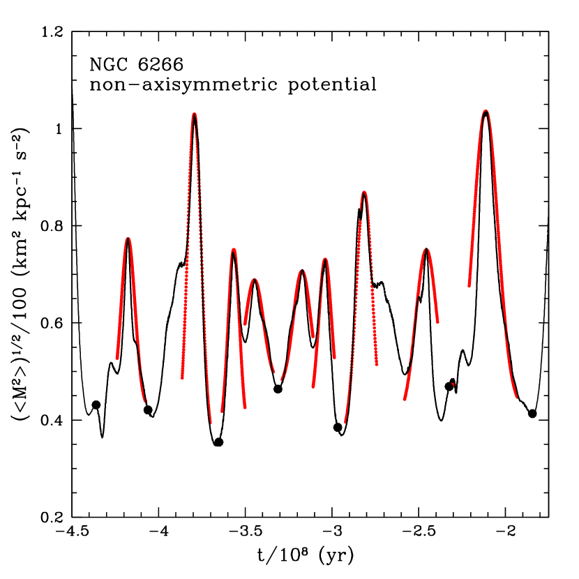
Figure 17: An example in the non-axisymmetric potential of the Gaussian fits to ($<$$M$${}^{2}>$)^1/2 in some apogalactic periods, where this tidal acceleration has more than one maximum in a given period. The black dots show the positions of the apogalactic points, and the red curves the approximate fits to the main peaks in the tidal acceleration.

In the axisymmetric potential the tidal acceleration ($<$$M$${}^{2}>$)^1/2 has one maximum in every apogalactic period. However, in the non-axisymmetric potential, and in some clusters, this acceleration may have a complicated behavior in some apogalactic periods, showing more than one maximum. Figure 17 shows as an example some apogalactic periods in a run in the cluster NGC 6266. The black dots give the positions in time of apogalactic points; the black curve is ($<$$M$${}^{2}>$)^1/2 and the red curves show the typical approximate fits made to the main acceleration peaks in cases like this.

Including the adiabatic correction factors, the averages of Eqs. (6) and (7) over the cluster are

$$<\!(\Delta E)_{b}\!>=\frac{1}{6}<\!r^{\prime 2}{\eta}_{1}(x(r^{\prime}))\!>\sum_{i,j}I^{2}_{ij},$$ (12)

$$<\!(\Delta E)_{b}^{2}\!>\approx\frac{1}{9}<\!r^{\prime 2}v^{\prime 2}(r^{\prime})(1+{\chi}_{r^{\prime},v^{\prime}}(r^{\prime})){\eta}_{2}(x(r^{\prime}))\!>\sum_{i,j}I^{2}_{ij},$$ (13)

with

$$<\!r^{\prime 2}{\eta}_{1}(x(r^{\prime}))\!>=\frac{4\pi}{M_{c}}\int_{0}^{r_{K}}{\rho}_{c}(r^{\prime}){\eta}_{1}(x(r^{\prime}))r^{\prime 4}dr^{\prime},$$ (14)

$$<\!r^{\prime 2}v^{\prime 2}(r^{\prime})(1+{\chi}_{r^{\prime},v^{\prime}}(r^{\prime})){\eta}_{2}(x(r^{\prime}))\!>=\frac{4{\pi}G}{M_{c}}\int_{0}^{r_{K}}{\rho}_{c}(r^{\prime})M_{c}(r^{\prime}){\eta}_{2}(x(r^{\prime}))(1+{\chi}_{r^{\prime},v^{\prime}}(r^{\prime}))r^{\prime 3}dr^{\prime},$$ (15)

and $<$$r_{c}^{2}$$>$ in Eq. (11)

$$<\!r_{c}^{2}\!>=<\!r^{\prime 2}\!>=\frac{4\pi}{M_{c}}\int_{0}^{r_{K}}{\rho}_{c}(r^{\prime})r^{\prime 4}dr^{\prime},$$ (16)

$r_{K}$ is the tidal radius of the cluster (listed in Table 1), $M_{c}$ is its total mass, ${\rho}_{c}(r^{\prime})$ is its spatial density, obtained with a King (1966) model, and $M_{c}(r^{\prime})$ is the mass of the cluster within radius $r^{\prime}$. As in Paper I, we approximate the rms velocity $v^{\prime}(r^{\prime})$ with the corresponding circular velocity at that $r^{\prime}$.

With $E_{c}\simeq-0.2GM_{c}/r_{h}$ the mean binding energy per unit mass of the cluster, and if the cluster has a dominant maximum of the tidal acceleration ($<$$M$${}^{2}>$)^1/2 in a given apogalactic period, bulge shock timescales in this period are defined as (Gnedin & Ostriker, 1997)

$$t_{bulge,1}=\left(\frac{-E_{c}}{<\!(\Delta E)_{b}\!>}\right)P_{orb},$$ (17)

$$t_{bulge,2}=\left(\frac{E_{c}^{2}}{<\!(\Delta E)_{b}^{2}\!>}\right)P_{orb},$$ (18)

with $P_{orb}$ the apogalactic period. If the cluster has more than one maximum of ($<$$M$${}^{2}>$)^1/2 in the given apogalactic period, as in Figure 10, instead of $P_{orb}$ we use in each main fitted peak the corresponding interval of time taken in the fit. In each case the total destruction rate due to bulge shocking is

$$\frac{1}{t_{bulge}}=\frac{1}{t_{bulge,1}}+\frac{1}{t_{bulge,2}}.$$ (19)

7 Disk and spiral arms shocking

The treatment for disk shocking remains the same as in Paper I. The corresponding expressions to Eqs. (12) and (13) for disk shocking are obtained averaging equations (1) and (2) in Gnedin et al. (1999b), resulting in

$$<\!(\Delta E)_{d}\!>=\frac{2g_{m}^{2}}{3v_{z}^{2}}<\!r^{\prime 2}{\eta}_{1}(x(r^{\prime}))\!>,$$ (20)

$$<\!(\Delta E)_{d}^{2}\!>=\frac{4g_{m}^{2}}{9v_{z}^{2}}<\!r^{\prime 2}v^{\prime 2}{\eta}_{2}(x(r^{\prime}))(1+{\chi}_{r^{\prime},v^{\prime}}(r^{\prime}))\!>.$$ (21)

In both, the axisymmetric and non-axisymmetric Galactic potentials, $|g_{m}|$ is the maximum acceleration produced by the corresponding axisymmetric disk component in its perpendicular z-direction, on the perpendicular line to the plane of the disk passing at the position where the cluster crosses the disk, and $|v_{z}|$ is the z-velocity of the cluster at this point. Here $\tau$ in $x(r^{\prime})={\omega}(r^{\prime}){\tau}$ is given by $\tau=|z_{m}|/|v_{z}|$, with $|z_{m}|$ the z-distance at which $|g_{m}|$ is reached.

With $n$ crossings of the cluster orbit with the Galactic plane, disk shock timescales and corresponding total destruction rate are given by

$$t_{disk,1}=\left(\frac{-E_{c}}{<\!(\Delta E)_{d}\!>}\right)\frac{P_{orb}}{n},$$ (22)

$$t_{disk,2}=\left(\frac{E_{c}^{2}}{<\!(\Delta E)_{d}^{2}\!>}\right)\frac{P_{orb}}{n},$$ (23)

$$\frac{1}{t_{disk}}=\frac{1}{t_{disk,1}}+\frac{1}{t_{disk,2}}.$$ (24)

In the non-axisymmetric potential, the spiral arms represent a plane mass distribution, analogous to the axisymmetric disk component, and also produce a shock on a cluster crossing the Galactic plane, with corresponding averaged diffusion coefficients $<\!(\Delta E)_{arms}\!>$ and $<\!(\Delta E)_{arms}^{2}\!>$ . At a given crossing point, the ratios $<\!(\Delta E)_{arms}\!>/<\!(\Delta E)_{d}\!>$, $<\!(\Delta E)_{arms}^{2}\!>/<\!(\Delta E)_{d}^{2}\!>$ between averaged diffusion coefficients due to the spiral arms and axisymmetric disk, will depend on the squared ratio of corresponding maximum accelerations $(|g_{m}|_{arms}/|g_{m}|_{disk})^{2}$. The velocity $|v_{z}|$ has the same value in both type of diffusion coefficients, as this velocity, as well as the orbit itself, is computed under the whole Galactic potential, i.e. including the axisymmetric (disk and dark halo) and non-axisymmetric (bar and spiral arms) components. There will be also a dependence of these ratios on the corresponding $|z_{m}|$ given by the spiral arms, through the dependence of ${\eta}_{1}$ and ${\eta}_{2}$ on $\tau$.

Figures 18 and 19 show the azimuth-averaged ratios $(|g_{m}|_{arms}/|g_{m}|_{disk})^{2}$ and $|z_{m}|_{arms}/|z_{m}|_{disk}$ as functions of the distance $R$ to the Galactic center of the point where a cluster orbit crosses the Galactic plane. The squared ratio $(|g_{m}|_{arms}/|g_{m}|_{disk})^{2}$ is important only in the region of the spiral arms (2-12 kpc) and of order $10^{-2}$-$10^{-3}$. In this region $|z_{m}|_{arms}/|z_{m}|_{disk}$ is close to unity. Thus, in our analysis we ignore the spiral arms shocking, which compared with the one of the disk will be two or three orders of magnitude lower.

8 Destruction rates. Results

In this section we present bulge-shocking destruction rates obtained with the formulism given in the last section, using the real trajectories of globular clusters in the employed Galactic potentials, and compare with corresponding values obtained with the usual linear trajectory approximation used in Paper I. The disk-shocking destruction rates are also computed and compared in the axisymmetric and non-axisymmetric potentials. All the computations are done with Monte Carlo simulations.

Table 4 shows our results. Bulge-shocking destruction rates averaged over the last $10^{9}$ yr in a cluster’s orbit (this time is increased in some clusters) and their lower, ${\sigma}_{-}$, and upper, ${\sigma}_{+}$, uncertainties, are listed according to the linear (columns 2-4) or real (columns 5-7) employed cluster’s trajectory. Columns 8-10 give the disk-shocking destruction rates. For each cluster, the first line gives values in the non-axisymmetric potential, and the second line in the axisymmetric potential.

With the data given in Table 4, Figures 20 and 21 show separately the comparison of bulge-shocking total destruction rates in the axisymmetric and non-axisymmetric Galactic potentials. Values obtained with the real trajectory of the cluster are shown in the vertical axis, and in the horizontal axis those with the linear trajectory. The error bars in these and following figures are given by the ${\sigma}_{-}$ and ${\sigma}_{+}$ values in Table 4. The conclusion from these two figures is that the use of the linear trajectory, along with the associated effective interaction time estimated as $\tau=|$$r$${}_{p}|/|$$v$${}_{p}|$, gives a good approximation to compute destruction rates due to the bulge, in the axisymmetric and non-axisymmetric Galactic potentials.

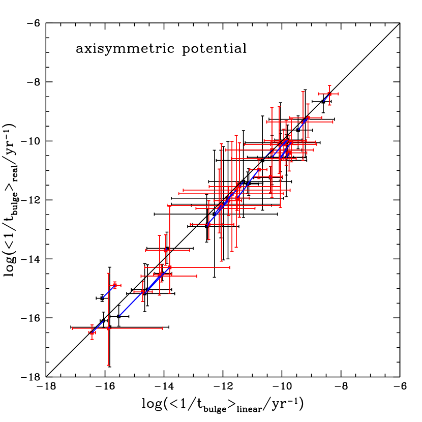
Figure 22: Comparison of bulge-shocking total destruction rates in the axisymmetric potential, employing the real and linear trajectories in each cluster. Here the cluster mass $M_{c}$ is computed with dynamical mass-to-light ratios $(M/L)_{V}$ given by McLaughlin & van der Marel (2005). Black points are points from Figure 20, and red points are the new points obtained with the dynamical mass-to-light ratios. Corresponding shifts between black and red points in a cluster are shown with blue lines.

To see how much the computed destruction rates can change if we take the cluster mass-to-light ratio $(M/L)_{V}$ different from the assumed $(M/L)_{V}$ = 2 $M_{\odot}/L_{\odot}$, we consider, as in Figure 12, dynamical mass-to-light ratios $(M/L)_{V}$ obtained by McLaughlin & van der Marel (2005). For clusters in common between our sample and in table 13 of McLaughlin & van der Marel (2005), the new cluster mass $M_{c}$ is computed, and in Figure 22 we show the comparison of bulge-shocking total destruction rates in particular in the axisymmetric potential, comparing values using the real (vertical axis) and linear (horizontal axis) trajectory. The black points with their uncertainties are points from Figure 20, obtained with the assumed $(M/L)_{V}$ = 2 $M_{\odot}/L_{\odot}$. The red points are obtained with the dynamical mass-to-light ratios given by McLaughlin & van der Marel (2005). The correspondig shifts between black and red points in a cluster are shown with blue lines. Thus, the destruction rates do not change too much, specially those with high values, and the standard $(M/L)_{V}$ = 2 $M_{\odot}/L_{\odot}$ is a convenient test value.

Taking the real trajectories, Figure 23 shows the comparison of bulge-shocking total destruction rates in the non-axisymmetric (vertical axis) and axisymmetric (horizontal axis) Galactic potentials. Here we note important differences between both potentials, specially in the region of high destruction rates, where values obtained with the non-axisymmetric potential are $smaller$ than those with the axisymmetric potential. As noted in $\S$ 3, in the non-axisymmetric potential all the bulge is represented by the Galactic bar; thus, there is no remnant of the original concentrated spherical bulge in the axisymmetric potential, whose mass is now distributed over the bar, with less central concentration (see upper frame in figure 7 in Paper I) and thus less dangerous for clusters crossing its region. This explains the behavior in the high destruction rate region in Figure 23. In $\S$ 5.1.1 we saw a related $decrease$ of tidal radii in the inner Galactic region in the non-axisymmetric potential; see discussion of Figure 8 in that section. Our conclusion is that the more appropriate non-axisymmetric Galactic potential employed in our computations, reduces the destruction rates due to the bulge (bar, in this case) for clusters with perigalacticons in the inner Galactic region.

Disk-shocking destruction rates in the non-axisymmetric and axisymmetric potentials are compared in Figure 24. Practically these destruction rates are the same in both potentials. Comparing this figure with Figure 23, we note that the disk dominates the destruction rate for clusters in the low destruction rate region, i.e. clusters with perigalacticons relatively distant from the Galactic center.

Adding the bulge-shocking total destruction rate obtained with the real trajectory of the cluster, and the disk-shocking destruction rate, results in the total bulge+disk destruction rate. Figure 25 shows the comparison of these total values in the non-axisymmetric (vertical axis) and axisymmetric (horizontal axis) Galactic potentials. In Figure 26 we show the same Figure 25 but now without the error bars. Empty and black squares correspond to clusters with orbital eccentricity $e\leq 0.5$ and $e>0.5$, respectively. The points marked with a circle show the clusters whose mass is less than $10^{5}M_{\odot}$. The position of some clusters are marked with their NGC and Pal numbers.

As in Figure 23, in these last figures we note that in the region of high destruction rates, dominated by the bulge, the total destruction rates obtained with the non-axisymmetric potential are $smaller$ than those resulting with the axisymmetric potential. Figure 26 shows that the majority of clusters with high eccentricities ($e>0.5$), have smaller destruction rates in the non-axisymmetric potential.

With the non-axisymmetric Galactic potential employed in our analysis, along with the more appropriate Monte Carlo simulations, we see from Figure 26 that seven clusters have particularly high destruction rates at the present time, due to bulge and disk shocking: Pal 5, NGC 6144, NGC 6121, NGC 6342, NGC 5897, NGC 6293, and NGC 6522. In Paper I, using only the Galactic bar in the non-axisymmetric potential, we found that NGC 6528 had the greatest destruction rate; now with the present non-axisymmetric Galactic model and the Monte Carlo simulations, this cluster has a low destruction rate, as shown in Figure 26.

9 Conclusions

We have employed the available 6-D data (positions and velocities) of 63 globular clusters in our Galaxy to analyze their Galactic orbits and compute their tidal radii, as well as their bulge and disk shocking destruction rates. This analysis has been made in axisymmetric and non-axisymmetric Galactic potentials; in particular, the used non-axisymmetric potential is a very detailed model which includes both the Galactic bar and a 3D model for the spiral arms. Our analysis is made using Monte Carlo simulations, to take into account the several uncertainties in the kinematical data of the clusters. For the computation of destruction rates due to the bulge in both Galactic potentials, we have employed the rigorous treatment of considering the real Galactic cluster orbit, instead of the usual linear trajectory employed in previous studies.

Our first result is that the theoretical tidal radius computed in the non-axisymmetric Galactic potential compares better with the observed tidal radius than that computed in the axisymmetric potential. This result leaves an open question with a recent study made by Webb et al. (2013), who propose a correction to be applied to the theoretical tidal radius computed at perigalacticon, to have a better comparison with the observed tidal radius. In our computations we do not need to introduce this correction.

The first conclusion from our results of bulge-shocking destruction rates is that the usual linear trajectory of the cluster considered at perigalacticon, gives a good approximation to the result obtained taking the real trajectory of the cluster. This conclusion holds in both the axisymmetric and non-axisymmetric potentials.

Our second conclusion is that the bulge-shocking destruction rates for clusters with perigalacticons in the inner Galactic region, turn out to be $smaller$ in the non-axisymmetric potential, as compared with those in the axisymmetric one. The majority of clusters with high orbital eccentricities ($e>0.5$) have $smaller$ total bulge+disk destruction rates in the non-axisymmetric potential.

We acknowledge financial support from UNAM DGAPA-PAPIIT through grant IN114114.

Table 1: Globular Clusters Data

Cluster	${\alpha}_{2000}$	${\delta}_{2000}$	$r$	$v_{r}$	${\mu}_{x}$	${\mu}_{y}$	$M_{c}$	$r_{K}$	$r_{h}$
	($deg$)	($deg$)	($kpc$)	($km/s$)	($mas$)	($mas$)	($M_{\odot}$)	($pc$)	($pc$)
NGC 104	6.02363	$-$72.08128	4.5$\pm$0.45	$-$18.0$\pm$0.1	5.64$\pm$0.20	$-$2.02$\pm$0.20	0.10E+07	55.37	4.15
NGC 288	13.18850	$-$26.58261	8.9$\pm$0.89	$-$45.4$\pm$0.2	4.67$\pm$0.42	$-$5.62$\pm$0.23	0.86E+05	34.15	5.77
NGC 362	15.80942	$-$70.84878	8.6$\pm$0.86	223.5$\pm$0.5	5.07$\pm$0.71	$-$2.55$\pm$0.72	0.40E+06	26.61	2.05
NGC 1851	78.52817	$-$40.04655	12.1$\pm$1.21	320.5$\pm$0.6	1.28$\pm$0.68	2.39$\pm$0.65	0.37E+06	22.95	1.80
NGC 1904	81.04621	$-$24.52472	12.9$\pm$1.29	205.8$\pm$0.4	2.12$\pm$0.64	$-$0.02$\pm$0.64	0.24E+06	30.90	2.44
NGC 2298	102.24754	$-$36.00531	10.8$\pm$1.08	148.9$\pm$1.2	4.05$\pm$1.00	$-$1.72$\pm$0.98	0.57E+05	23.36	3.08
NGC 2808	138.01292	$-$64.86350	9.6$\pm$0.96	101.6$\pm$0.7	0.58$\pm$0.45	2.06$\pm$0.46	0.97E+06	25.35	2.23
Pal 3	151.38292	0.07167	92.5$\pm$9.25	83.4$\pm$8.4	0.33$\pm$0.23	0.30$\pm$0.31	0.32E+05	107.81	17.49
NGC 3201	154.40342	$-$46.41247	4.9$\pm$0.49	494.0$\pm$0.2	5.28$\pm$0.32	$-$0.98$\pm$0.33	0.16E+06	36.13	4.42
NGC 4147	182.52625	18.54264	19.3$\pm$1.93	183.2$\pm$0.7	$-$1.85$\pm$0.82	$-$1.30$\pm$0.82	0.50E+05	34.16	2.69
NGC 4372	186.43917	$-$72.65900	5.8$\pm$0.58	72.3$\pm$1.2	$-$6.49$\pm$0.33	3.71$\pm$0.32	0.22E+06	58.91	6.60
NGC 4590	189.86658	$-$26.74406	10.3$\pm$1.03	$-$94.7$\pm$0.2	$-$3.76$\pm$0.66	1.79$\pm$0.62	0.15E+06	44.67	4.52
NGC 4833	194.89133	$-$70.87650	6.6$\pm$0.66	200.2$\pm$1.2	$-$8.11$\pm$0.35	$-$0.96$\pm$0.34	0.32E+06	34.14	4.63
NGC 5024	198.23021	18.16817	17.9$\pm$1.79	$-$62.9$\pm$0.3	0.50$\pm$1.00	$-$0.10$\pm$1.00	0.52E+06	95.64	6.82
NGC 5139	201.69683	$-$47.47958	5.2$\pm$0.52	232.1$\pm$0.1	$-$5.08$\pm$0.35	$-$3.57$\pm$0.34	0.22E+07	73.19	7.56
NGC 5272	205.54842	28.37728	10.2$\pm$1.02	$-$147.6$\pm$0.2	$-$1.10$\pm$0.51	$-$2.30$\pm$0.54	0.61E+06	85.22	6.85
NGC 5466	211.36371	28.53444	16.0$\pm$1.60	110.7$\pm$0.2	$-$4.65$\pm$0.82	0.80$\pm$0.82	0.11E+06	72.98	10.70
Pal 5	229.02188	$-$0.11161	23.2$\pm$2.32	$-$58.7$\pm$0.2	$-$1.78$\pm$0.17	$-$2.32$\pm$0.23	0.20E+05	51.17	18.42
NGC 5897	229.35208	$-$21.01028	12.5$\pm$1.25	101.5$\pm$1.0	$-$4.93$\pm$0.86	$-$2.33$\pm$0.84	0.13E+06	36.88	7.49
NGC 5904	229.63842	2.08103	7.5$\pm$0.75	53.2$\pm$0.4	5.07$\pm$0.68	$-$10.70$\pm$0.56	0.57E+06	51.55	3.86
NGC 5927	232.00288	$-$50.67303	7.7$\pm$0.77	$-$107.5$\pm$0.9	$-$5.72$\pm$0.39	$-$2.61$\pm$0.40	0.23E+06	37.45	2.46
NGC 5986	236.51250	$-$37.78642	10.4$\pm$1.04	88.9$\pm$3.7	$-$3.81$\pm$0.45	$-$2.99$\pm$0.37	0.41E+06	24.15	2.96
NGC 6093	244.26004	$-$22.97608	10.0$\pm$1.00	8.1$\pm$1.5	$-$3.31$\pm$0.58	$-$7.20$\pm$0.67	0.33E+06	20.88	1.77
NGC 6121	245.89675	$-$26.52575	2.2$\pm$0.22	70.7$\pm$0.2	$-$12.50$\pm$0.36	$-$19.93$\pm$0.49	0.13E+06	33.16	2.77
NGC 6144	246.80775	$-$26.02350	8.9$\pm$0.89	193.8$\pm$0.6	$-$3.06$\pm$0.64	$-$5.11$\pm$0.72	0.94E+05	86.35	4.22
NGC 6171	248.13275	$-$13.05378	6.4$\pm$0.64	$-$34.1$\pm$0.3	$-$0.70$\pm$0.90	$-$3.10$\pm$1.00	0.12E+06	35.33	3.22
NGC 6205	250.42183	36.45986	7.1$\pm$0.71	$-$244.2$\pm$0.2	$-$0.90$\pm$0.71	5.50$\pm$1.12	0.45E+06	43.39	3.49
NGC 6218	251.80908	$-$1.94853	4.8$\pm$0.48	$-$41.4$\pm$0.2	1.30$\pm$0.58	$-$7.83$\pm$0.62	0.14E+06	24.13	2.47
NGC 6254	254.28771	$-$4.10031	4.4$\pm$0.44	75.2$\pm$0.7	$-$6.00$\pm$1.00	$-$3.30$\pm$1.00	0.17E+06	23.64	2.50
NGC 6266	255.30333	$-$30.11372	6.8$\pm$0.68	$-$70.1$\pm$1.4	$-$3.50$\pm$0.37	$-$0.82$\pm$0.37	0.80E+06	23.10	1.82
NGC 6273	255.65750	$-$26.26797	8.8$\pm$0.88	135.0$\pm$4.1	$-$2.86$\pm$0.49	$-$0.45$\pm$0.51	0.77E+06	37.30	3.38
NGC 6284	256.11879	$-$24.76486	15.3$\pm$1.53	27.5$\pm$1.7	$-$3.66$\pm$0.64	$-$5.39$\pm$0.83	0.26E+06	102.72	2.94
NGC 6287	256.28804	$-$22.70836	9.4$\pm$0.94	$-$288.7$\pm$3.5	$-$3.68$\pm$0.88	$-$3.54$\pm$0.69	0.15E+06	19.02	2.02
NGC 6293	257.54250	$-$26.58208	9.5$\pm$0.95	$-$146.2$\pm$1.7	0.26$\pm$0.85	$-$5.14$\pm$0.71	0.22E+06	39.32	2.46
NGC 6304	258.63438	$-$29.46203	5.9$\pm$0.59	$-$107.3$\pm$3.6	$-$2.59$\pm$0.29	$-$1.56$\pm$0.29	0.14E+06	22.74	2.44
NGC 6316	259.15542	$-$28.14011	10.4$\pm$1.04	71.4$\pm$8.9	$-$2.42$\pm$0.63	$-$1.71$\pm$0.56	0.37E+06	22.97	1.97
NGC 6333	259.79692	$-$18.51594	7.9$\pm$0.79	229.1$\pm$7.0	$-$0.57$\pm$0.57	$-$3.70$\pm$0.50	0.26E+06	18.39	2.21
NGC 6341	259.28079	43.13594	8.3$\pm$0.83	$-$120.0$\pm$0.1	$-$3.30$\pm$0.55	$-$0.33$\pm$0.70	0.33E+06	30.05	2.46
NGC 6342	260.29200	$-$19.58742	8.5$\pm$0.85	115.7$\pm$1.4	$-$2.77$\pm$0.71	$-$5.84$\pm$0.65	0.63E+05	36.74	1.80
NGC 6356	260.89554	$-$17.81303	15.1$\pm$1.51	27.0$\pm$4.3	$-$3.14$\pm$0.68	$-$3.65$\pm$0.53	0.43E+06	41.01	3.56
NGC 6362	262.97913	$-$67.04833	7.6$\pm$0.76	$-$13.1$\pm$0.6	$-$3.09$\pm$0.46	$-$3.83$\pm$0.46	0.10E+06	30.73	4.53
NGC 6388	264.07179	$-$44.73550	9.9$\pm$0.99	80.1$\pm$0.8	$-$1.90$\pm$0.45	$-$3.83$\pm$0.51	0.99E+06	19.43	1.50
NGC 6397	265.17538	$-$53.67433	2.3$\pm$0.23	18.8$\pm$0.1	3.69$\pm$0.29	$-$14.88$\pm$0.26	0.77E+05	29.79	1.94
NGC 6441	267.55442	$-$37.05144	11.6$\pm$1.16	16.5$\pm$1.0	$-$2.86$\pm$0.45	$-$3.45$\pm$0.76	0.12E+07	24.11	1.92
NGC 6522	270.89175	$-$30.03397	7.7$\pm$0.77	$-$21.1$\pm$3.4	6.08$\pm$0.20	$-$1.83$\pm$0.20	0.20E+06	36.82	2.24
NGC 6528	271.20683	$-$30.05628	7.9$\pm$0.79	206.6$\pm$1.4	$-$0.35$\pm$0.23	0.27$\pm$0.26	0.73E+05	9.45	0.87
NGC 6553	272.32333	$-$25.90869	6.0$\pm$0.60	$-$3.2$\pm$1.5	2.50$\pm$0.07	5.35$\pm$0.08	0.22E+06	13.37	1.80
NGC 6584	274.65667	$-$52.21578	13.5$\pm$1.35	222.9$\pm$15.0	$-$0.22$\pm$0.62	$-$5.79$\pm$0.67	0.20E+06	30.13	2.87
NGC 6626	276.13671	$-$24.86978	5.5$\pm$0.55	17.0$\pm$1.0	0.63$\pm$0.67	$-$8.46$\pm$0.67	0.31E+06	17.96	3.15
NGC 6656	279.09975	$-$23.90475	3.2$\pm$0.32	$-$146.3$\pm$0.2	7.37$\pm$0.50	$-$3.95$\pm$0.42	0.43E+06	29.70	3.13
NGC 6712	283.26792	$-$8.70611	6.9$\pm$0.69	$-$107.6$\pm$0.5	4.20$\pm$0.40	$-$2.00$\pm$0.40	0.17E+06	17.12	2.67
NGC 6723	284.88813	$-$36.63225	8.7$\pm$0.87	$-$94.5$\pm$3.6	$-$0.17$\pm$0.45	$-$2.16$\pm$0.50	0.23E+06	30.20	3.87
NGC 6752	287.71712	$-$59.98456	4.0$\pm$0.40	$-$26.7$\pm$0.2	$-$0.69$\pm$0.42	$-$2.85$\pm$0.45	0.21E+06	40.48	2.22
NGC 6779	289.14821	30.18347	9.4$\pm$0.94	$-$135.6$\pm$0.9	0.30$\pm$1.00	1.40$\pm$0.10	0.16E+06	28.86	3.01
NGC 6809	294.99879	$-$30.96475	5.4$\pm$0.54	174.7$\pm$0.3	$-$1.42$\pm$0.62	$-$10.25$\pm$0.64	0.18E+06	24.07	4.45
NGC 6838	298.44371	18.77919	4.0$\pm$0.40	$-$22.8$\pm$0.2	$-$2.30$\pm$0.80	$-$5.10$\pm$0.80	0.30E+05	10.35	1.94
NGC 6934	308.54738	7.40447	15.6$\pm$1.56	$-$411.4$\pm$1.6	1.20$\pm$1.00	$-$5.10$\pm$1.00	0.16E+06	33.83	3.13
NGC 7006	315.37242	16.18733	41.2$\pm$4.12	$-$384.1$\pm$0.4	$-$0.96$\pm$0.35	$-$1.14$\pm$0.40	0.20E+06	52.37	5.27
NGC 7078	322.49304	12.16700	10.4$\pm$1.04	$-$107.0$\pm$0.2	$-$0.95$\pm$0.51	$-$5.63$\pm$0.50	0.81E+06	63.23	3.03
NGC 7089	323.36258	$-$0.82325	11.5$\pm$1.15	$-$5.3$\pm$2.0	5.90$\pm$0.86	$-$4.95$\pm$0.86	0.70E+06	41.65	3.55
NGC 7099	325.09217	$-$23.17986	8.1$\pm$0.81	$-$184.2$\pm$0.2	1.42$\pm$0.69	$-$7.71$\pm$0.65	0.16E+06	37.43	2.43
Pal 12	326.66183	$-$21.25261	19.0$\pm$1.90	27.8$\pm$1.5	$-$1.20$\pm$0.30	$-$4.21$\pm$0.29	0.10E+05	105.56	9.51
Pal 13	346.68517	12.77200	26.0$\pm$2.60	25.2$\pm$0.3	2.30$\pm$0.26	0.27$\pm$0.25	0.54E+04	16.59	2.72

Table 2: Galactic parameters

Parameter	Value	References
$R_{0}$	8.3$\pm$0.23 kpc	1
${\Theta}_{0}$	239$\pm$7 km/s	1
$(U,V,W)_{\odot}$	($-11.1\pm$1.2,12.24$\pm$2.1,7.25$\pm$0.6) km s-1	2,1
Galactic Bar
position of major axis	20∘	3
angular velocity	55$\pm$5 ${\rm\,km\,s^{-1}{kpc}^{-1}}$	4
Spiral Arms
$M_{\rm arms}/M_{\rm disk}$	0.04$\pm$0.01	5
scale length ($H$)	3.9$\pm$0.6 kpc ($R_{0}$ = 8.5 kpc)	6
pitch angle	15.5$\pm$3.5∘	7
angular velocity	24$\pm$6 ${\rm\,km\,s^{-1}{kpc}^{-1}}$	4

References. — 1) Brunthaler et al. (2011). 2) Schönrich et al. (2010). 3) Gerhard (2002). 4) Gerhard (2011). 5) Pichardo et al. (2012). 6) Benjamin et al. (2005). 7) Drimmel (2000).

Table 3: Orbital parameters with the non-axisymmetric and axisymmetric potentials

Cluster	$<$$r_{min}$$>$	$<$$r_{max}$$>$	$<$$|z|_{max}$$>$	$<$$e$$>$	$E$	$h$	$<$$r_{K_{t}}$$>$	$<$$r_{\ast}$$>$
	($kpc$)	($kpc$)	($kpc$)		(10$kms^{-1})^{2}$	(10$kms^{-1}kpc$)	($pc$)	($pc$)
NGC 104	5.78	8.30	3.13	0.177			91.6	102.9
	6.25	7.57	3.16	0.095	$-1482.12$	134.55	98.3	112.4
NGC 288	2.60	12.38	6.40	0.654			23.6	22.8
	2.78	12.25	6.70	0.632	$-1384.68$	$-46.38$	24.5	23.5
NGC 362	1.39	9.28	3.85	0.736			24.3	20.7
	0.74	11.09	2.16	0.877	$-1492.42$	$-12.56$	17.1	15.9
NGC 1851	6.66	33.28	7.61	0.667			70.1	68.2
	6.73	31.75	7.59	0.650	$-939.52$	238.99	71.5	69.5
NGC 1904	5.25	18.85	5.54	0.563			51.4	51.4
	5.19	20.52	5.37	0.596	$-1137.89$	173.68	52.0	51.6
NGC 2298	3.18	20.38	11.49	0.731			22.0	20.8
	3.20	17.90	9.52	0.698	$-1212.81$	$-56.36$	22.7	21.3
NGC 2808	2.27	10.74	2.39	0.649			46.0	43.4
	2.73	12.74	2.59	0.647	$-1395.39$	94.19	53.3	51.4
NGC 3201	9.00	16.86	4.54	0.304			67.5	72.3
	8.99	17.12	4.52	0.311	$-1151.30$	$-251.56$	67.8	72.5
NGC 4147	3.89	27.33	13.97	0.750			25.0	22.8
	3.78	28.64	14.73	0.766	$-1001.35$	66.83	25.4	22.8
NGC 4372	2.39	5.30	1.57	0.386			30.4	33.2
	3.19	7.41	1.60	0.397	$-1624.75$	95.34	37.7	39.9
NGC 4590	9.60	30.81	11.86	0.525			67.5	68.6
	9.57	30.40	11.82	0.521	$-932.42$	264.42	68.0	68.6
NGC 4833	1.04	8.41	1.54	0.778			22.1	18.3
	0.98	7.43	1.93	0.767	$-1685.97$	26.11	18.3	17.3
NGC 5024	16.43	36.30	24.34	0.377			155.4	161.6
	16.44	36.46	24.44	0.379	$-811.52$	143.90	155.7	161.9
NGC 5139	1.49	5.81	1.69	0.592			47.5	47.4
	0.98	6.45	1.16	0.737	$-1770.34$	$-34.25$	36.7	35.5
NGC 5272	5.61	13.28	8.77	0.404			76.3	80.2
	5.60	14.22	8.99	0.435	$-1267.90$	79.36	76.7	79.4
NGC 5466	6.81	60.45	36.45	0.797			48.8	44.1
	6.85	60.20	36.33	0.796	$-663.05$	$-32.56$	49.1	44.2
Pal 5	3.80	18.74	10.93	0.663			19.2	18.5
	3.97	18.88	10.92	0.653	$-1179.26$	54.78	19.6	18.7
NGC 5897	1.89	7.95	5.09	0.621			23.4	22.5
	1.48	8.94	4.49	0.719	$-1552.41$	23.18	17.5	16.6
NGC 5904	2.65	36.80	17.89	0.866			46.5	40.4
	2.76	37.35	18.11	0.863	$-888.65$	40.12	46.6	40.5
NGC 5927	3.44	4.64	0.80	0.150			41.4	48.8
	4.50	5.45	0.79	0.095	$-1693.39$	110.15	48.7	57.3
NGC 5986	1.05	3.97	1.33	0.562			24.7	24.6
	0.46	4.90	1.31	0.831	$-1904.82$	1.51	12.9	12.4
NGC 6093	2.07	3.11	3.02	0.201			34.1	37.0
	2.01	3.78	3.14	0.311	$-1867.55$	10.18	31.7	32.8
NGC 6121	0.39	5.95	0.49	0.874			11.6	7.7
	0.55	5.47	2.11	0.827	$-1824.59$	$-1.58$	9.8	8.7
NGC 6144	2.14	2.99	2.64	0.166			22.2	24.9
	2.08	2.66	2.33	0.123	$-1981.75$	$-20.51$	22.1	23.3
NGC 6171	2.28	3.14	2.34	0.157			25.1	28.4
	2.70	3.31	2.41	0.104	$-1886.70$	39.42	28.3	31.2
NGC 6205	5.35	21.93	13.90	0.609			67.7	67.2
	5.30	22.61	14.22	0.621	$-1087.59$	$-30.31$	67.1	66.4
NGC 6218	2.76	5.94	2.21	0.363			30.0	32.1
	2.73	5.32	2.56	0.323	$-1744.69$	59.13	29.5	31.2
NGC 6254	3.86	5.84	2.43	0.204			38.8	43.5
	3.46	4.93	2.40	0.175	$-1737.04$	71.23	37.3	41.9
NGC 6266	1.52	2.63	0.83	0.276			37.2	43.6
	1.41	2.22	0.85	0.223	$-2167.78$	33.20	32.8	34.9
NGC 6273	1.28	2.40	1.28	0.304			34.4	38.4
	1.35	1.83	1.60	0.153	$-2169.73$	$-11.81$	32.0	33.2
NGC 6284	6.34	8.52	2.78	0.147			62.2	69.7
	6.40	8.10	2.68	0.117	$-1461.17$	148.72	64.3	73.3
NGC 6287	0.91	5.03	2.82	0.707			16.3	14.2
	0.87	4.30	2.44	0.671	$-1895.79$	$-3.07$	8.7	7.7
NGC 6293	0.32	3.34	0.46	0.826			14.2	8.9
	0.37	2.67	1.19	0.756	$-2168.38$	$-3.58$	8.6	7.7
NGC 6304	1.90	3.25	0.53	0.276			23.7	27.4
	1.84	3.09	0.57	0.253	$-2054.85$	48.88	22.8	24.3
NGC 6316	0.72	3.07	1.18	0.626			19.9	19.2
	0.96	2.59	0.83	0.460	$-2170.75$	$-26.10$	18.2	19.0
NGC 6333	1.44	5.32	1.53	0.582			21.5	21.5
	1.02	4.37	1.34	0.623	$-1937.01$	27.83	15.3	15.1
NGC 6341	1.20	10.43	2.43	0.793			22.9	20.6
	1.30	10.86	2.59	0.786	$-1496.54$	30.29	21.6	20.1
NGC 6342	1.29	2.09	1.37	0.245			14.9	17.1
	0.73	1.68	1.13	0.401	$-2304.73$	10.92	8.3	8.6
NGC 6356	2.45	7.94	2.08	0.528			38.2	39.6
	2.30	7.74	1.98	0.542	$-1637.01$	67.45	37.3	37.8
NGC 6362	2.31	5.05	1.98	0.374			22.4	24.0
	2.28	5.80	1.70	0.436	$-1760.08$	62.23	23.4	24.4
NGC 6388	0.70	3.03	1.10	0.627			27.6	26.1
	0.53	2.95	0.88	0.696	$-2148.65$	$-13.57$	16.2	16.2
NGC 6397	2.53	5.12	1.46	0.344			23.1	25.4
	3.33	6.42	1.66	0.317	$-1672.42$	91.10	27.4	29.7
NGC 6441	0.57	3.97	0.87	0.751			27.6	22.5
	0.48	3.15	1.45	0.742	$-2082.24$	$-2.77$	16.9	15.7
NGC 6522	0.37	3.87	0.57	0.831			13.4	8.9
	0.81	2.23	1.16	0.471	$-2199.97$	18.26	13.2	13.4
NGC 6528	0.81	2.85	1.20	0.571			12.5	12.0
	0.57	1.51	0.77	0.454	$-2399.18$	14.31	7.3	7.6
NGC 6553	2.09	8.75	0.33	0.615			28.9	28.1
	2.31	12.02	0.52	0.677	$-1445.87$	97.14	30.2	28.0
NGC 6584	1.38	12.43	4.43	0.804			21.7	19.4
	1.06	12.20	3.11	0.843	$-1434.63$	24.27	15.3	14.5
NGC 6626	1.03	2.82	0.85	0.472			21.7	24.0
	0.74	3.09	0.88	0.613	$-2111.49$	21.96	14.2	14.3
NGC 6656	2.85	7.96	1.18	0.472			42.9	45.1
	3.10	9.18	1.28	0.495	$-1542.68$	105.56	45.7	46.8
NGC 6712	0.60	5.56	1.14	0.809			15.9	13.6
	0.91	6.34	1.86	0.749	$-1767.49$	13.60	12.9	12.5
NGC 6723	2.00	3.25	3.03	0.242			29.1	31.4
	2.06	2.66	2.65	0.127	$-1969.12$	$-0.19$	30.1	30.8
NGC 6752	4.65	6.71	1.75	0.180			45.8	52.7
	4.74	5.81	1.72	0.102	$-1640.42$	109.14	48.9	56.8
NGC 6779	0.62	12.52	0.77	0.906			15.2	10.7
	0.84	12.49	2.44	0.875	$-1428.17$	$-24.15$	11.7	10.5
NGC 6809	1.98	5.95	3.87	0.508			25.5	26.1
	1.78	5.61	3.59	0.526	$-1741.44$	19.74	22.9	22.7
NGC 6838	5.01	6.56	0.33	0.131			25.2	29.4
	4.88	6.98	0.29	0.177	$-1599.94$	134.92	25.8	29.6
NGC 6934	6.88	34.87	20.35	0.670			54.6	52.3
	6.83	35.12	20.60	0.674	$-892.95$	$-56.25$	54.6	52.4
NGC 7006	17.89	79.15	26.93	0.631			115.4	111.1
	17.90	79.32	26.97	0.632	$-514.26$	572.52	115.7	111.4
NGC 7078	6.12	10.89	5.25	0.281			91.5	98.5
	6.48	11.00	5.45	0.259	$-1347.69$	139.60	94.4	103.1
NGC 7089	6.10	33.12	18.03	0.689			83.4	78.9
	6.14	34.19	18.77	0.695	$-908.90$	$-67.44$	84.1	79.3
NGC 7099	3.16	6.91	4.20	0.373			32.6	35.0
	3.09	7.38	4.70	0.412	$-1584.65$	$-46.62$	32.9	34.0
Pal 12	15.19	19.64	15.76	0.128			40.3	44.7
	15.25	19.86	15.90	0.131	$-1010.08$	165.80	40.4	44.8
Pal 13	11.84	88.01	38.03	0.763			25.4	23.5
	11.86	88.13	38.24	0.763	$-485.90$	$-329.53$	25.5	23.6

Table 4: Destruction Rates of globular clusters in the non-axisymmetric and axisymmetric potentials, obtained with Monte Carlo simulations

	———– Linear Trajectory ———–			———— Real Trajectory ————
Cluster	$<$$1/t_{bulge}$$>$	${\sigma}_{-}$	${\sigma}_{+}$	$<$$1/t_{bulge}$$>$	${\sigma}_{-}$	${\sigma}_{+}$	$<$$1/t_{disk}$$>$	${\sigma}_{-}$	${\sigma}_{+}$
	($yr^{-1}$)	($yr^{-1}$)	($yr^{-1}$)	($yr^{-1}$)	($yr^{-1}$)	($yr^{-1}$)	($yr^{-1}$)	($yr^{-1}$)	($yr^{-1}$)
NGC 104	0.321E-15	0.191E-15	0.962E-14	0.286E-14	0.225E-14	0.650E-14	0.146E-12	0.359E-13	0.616E-13
	0.806E-16	0.304E-16	0.497E-16	0.466E-15	0.104E-15	0.165E-15	0.148E-12	0.281E-13	0.352E-13
NGC 288	0.750E-10	0.669E-10	0.289E-09	0.157E-09	0.129E-09	0.408E-09	0.809E-11	0.440E-11	0.563E-11
	0.621E-09	0.585E-09	0.538E-08	0.542E-09	0.516E-09	0.496E-08	0.899E-11	0.493E-11	0.842E-11
NGC 362	0.365E-11	0.259E-11	0.445E-11	0.228E-11	0.144E-11	0.244E-11	0.128E-12	0.383E-13	0.439E-13
	0.767E-10	0.580E-10	0.134E-09	0.390E-10	0.301E-10	0.672E-10	0.170E-12	0.528E-13	0.614E-13
NGC 1851	0.540E-16	0.495E-16	0.227E-14	0.248E-15	0.236E-15	0.703E-14	0.777E-15	0.642E-15	0.332E-14
	0.145E-15	0.138E-15	0.146E-13	0.488E-16	0.466E-16	0.523E-14	0.860E-15	0.723E-15	0.419E-14
NGC 1904	0.127E-12	0.123E-12	0.306E-11	0.135E-12	0.126E-12	0.126E-11	0.628E-13	0.506E-13	0.164E-12
	0.105E-11	0.104E-11	0.866E-10	0.714E-12	0.704E-12	0.639E-10	0.635E-13	0.512E-13	0.176E-12
NGC 2298	0.789E-11	0.741E-11	0.469E-10	0.983E-11	0.889E-11	0.465E-10	0.835E-12	0.668E-12	0.151E-11
	0.769E-10	0.743E-10	0.834E-09	0.562E-10	0.544E-10	0.645E-09	0.989E-12	0.768E-12	0.182E-11
NGC 2808	0.498E-14	0.383E-14	0.201E-13	0.819E-14	0.666E-14	0.459E-13	0.727E-14	0.289E-14	0.406E-14
	0.225E-14	0.171E-14	0.210E-13	0.672E-15	0.510E-15	0.636E-14	0.537E-14	0.220E-14	0.328E-14
Pal 3	0.506E-15	0.499E-15	0.830E-14	0.154E-14	0.149E-14	0.239E-13	0.132E-14	0.129E-14	0.203E-13
	0.163E-14	0.161E-14	0.826E-13	0.107E-14	0.106E-14	0.556E-13	0.490E-14	0.483E-14	0.241E-12
NGC 3201	0.903E-16	0.221E-16	0.331E-16	0.168E-15	0.999E-16	0.174E-14	0.107E-13	0.504E-14	0.125E-13
	0.895E-16	0.212E-16	0.302E-16	0.801E-16	0.345E-16	0.779E-16	0.109E-13	0.505E-14	0.133E-13
NGC 4147	0.320E-11	0.308E-11	0.300E-10	0.300E-11	0.276E-11	0.209E-10	0.466E-12	0.384E-12	0.984E-12
	0.219E-10	0.213E-10	0.669E-09	0.217E-10	0.213E-10	0.685E-09	0.519E-12	0.427E-12	0.164E-11
NGC 4372	0.910E-10	0.697E-10	0.463E-09	0.670E-10	0.458E-10	0.234E-09	0.792E-10	0.327E-10	0.567E-10
	0.352E-11	0.167E-11	0.213E-11	0.238E-11	0.106E-11	0.136E-11	0.436E-10	0.137E-10	0.171E-10
NGC 4590	0.299E-15	0.149E-15	0.337E-15	0.147E-15	0.655E-16	0.258E-15	0.151E-13	0.887E-14	0.223E-13
	0.295E-15	0.145E-15	0.351E-15	0.112E-15	0.590E-16	0.154E-15	0.162E-13	0.951E-14	0.247E-13
NGC 4833	0.661E-10	0.408E-10	0.792E-10	0.160E-09	0.878E-10	0.144E-09	0.389E-11	0.107E-11	0.152E-11
	0.454E-09	0.326E-09	0.106E-08	0.264E-09	0.189E-09	0.633E-09	0.422E-11	0.100E-11	0.126E-11
NGC 5024	0.188E-12	0.187E-12	0.415E-10	0.487E-12	0.484E-12	0.597E-10	0.491E-13	0.475E-13	0.138E-11
	0.307E-12	0.305E-12	0.937E-10	0.292E-12	0.291E-12	0.104E-09	0.561E-13	0.539E-13	0.151E-11
NGC 5139	0.371E-10	0.187E-10	0.443E-10	0.958E-10	0.546E-10	0.105E-09	0.639E-11	0.157E-11	0.184E-11
	0.156E-09	0.992E-10	0.320E-09	0.108E-09	0.754E-10	0.241E-09	0.746E-11	0.151E-11	0.189E-11
NGC 5272	0.438E-12	0.377E-12	0.718E-11	0.170E-11	0.161E-11	0.221E-10	0.118E-11	0.618E-12	0.124E-11
	0.854E-12	0.770E-12	0.441E-10	0.661E-12	0.609E-12	0.481E-10	0.127E-11	0.681E-12	0.132E-11
NGC 5466	0.538E-11	0.503E-11	0.136E-09	0.171E-10	0.153E-10	0.247E-09	0.307E-11	0.245E-11	0.113E-10
	0.495E-11	0.462E-11	0.208E-09	0.417E-11	0.392E-11	0.221E-09	0.288E-11	0.227E-11	0.101E-10
Pal 5	0.345E-08	0.312E-08	0.149E-07	0.110E-07	0.950E-08	0.445E-07	0.461E-09	0.317E-09	0.516E-09
	0.304E-07	0.289E-07	0.300E-06	0.399E-07	0.383E-07	0.406E-06	0.616E-09	0.428E-09	0.172E-08
NGC 5897	0.250E-09	0.220E-09	0.625E-09	0.406E-09	0.366E-09	0.108E-08	0.196E-10	0.113E-10	0.154E-10
	0.434E-08	0.402E-08	0.218E-07	0.378E-08	0.354E-08	0.198E-07	0.246E-10	0.146E-10	0.280E-10
NGC 5904	0.350E-12	0.244E-12	0.853E-12	0.499E-12	0.393E-12	0.170E-11	0.189E-12	0.976E-13	0.190E-12
	0.302E-12	0.208E-12	0.631E-12	0.149E-12	0.104E-12	0.342E-12	0.198E-12	0.102E-12	0.192E-12
NGC 5927	0.535E-11	0.467E-11	0.473E-10	0.142E-11	0.118E-11	0.106E-10	0.483E-11	0.220E-11	0.324E-11
	0.255E-14	0.146E-14	0.506E-14	0.116E-13	0.395E-14	0.620E-14	0.156E-11	0.445E-12	0.564E-12
NGC 5986	0.222E-10	0.121E-10	0.187E-10	0.233E-10	0.151E-10	0.204E-10	0.523E-12	0.144E-12	0.172E-12
	0.640E-09	0.437E-09	0.564E-09	0.228E-09	0.155E-09	0.174E-09	0.605E-12	0.147E-12	0.171E-12
NGC 6093	0.194E-11	0.180E-11	0.735E-11	0.248E-11	0.232E-11	0.900E-11	0.128E-12	0.743E-13	0.872E-13
	0.140E-09	0.136E-09	0.332E-09	0.487E-10	0.474E-10	0.116E-09	0.156E-12	0.873E-13	0.112E-12
NGC 6121	0.286E-09	0.144E-09	0.167E-09	0.676E-09	0.310E-09	0.786E-09	0.176E-10	0.416E-11	0.651E-11
	0.252E-08	0.147E-08	0.219E-08	0.215E-08	0.125E-08	0.180E-08	0.137E-10	0.288E-11	0.372E-11
NGC 6144	0.126E-08	0.678E-09	0.206E-08	0.304E-08	0.161E-08	0.575E-08	0.325E-09	0.986E-10	0.862E-10
	0.226E-08	0.157E-08	0.182E-07	0.495E-08	0.249E-08	0.272E-07	0.472E-09	0.128E-09	0.176E-09
NGC 6171	0.206E-10	0.135E-10	0.468E-10	0.229E-10	0.140E-10	0.840E-10	0.170E-10	0.450E-11	0.486E-11
	0.897E-10	0.840E-10	0.188E-08	0.866E-10	0.775E-10	0.189E-08	0.177E-10	0.470E-11	0.604E-11
NGC 6205	0.325E-14	0.241E-14	0.300E-13	0.388E-13	0.342E-13	0.577E-12	0.611E-13	0.331E-13	0.931E-13
	0.277E-14	0.198E-14	0.156E-13	0.920E-15	0.662E-15	0.542E-14	0.657E-13	0.354E-13	0.813E-13
NGC 6218	0.260E-11	0.219E-11	0.183E-10	0.140E-11	0.115E-11	0.141E-10	0.136E-11	0.549E-12	0.870E-12
	0.280E-12	0.216E-12	0.323E-11	0.126E-12	0.889E-13	0.142E-11	0.123E-11	0.332E-12	0.454E-12
NGC 6254	0.821E-12	0.737E-12	0.714E-11	0.315E-12	0.258E-12	0.544E-11	0.777E-12	0.424E-12	0.679E-12
	0.127E-13	0.100E-13	0.859E-13	0.228E-13	0.157E-13	0.587E-13	0.584E-12	0.206E-12	0.308E-12
NGC 6266	0.594E-12	0.470E-12	0.341E-11	0.245E-12	0.158E-12	0.268E-12	0.781E-13	0.290E-13	0.418E-13
	0.130E-11	0.118E-11	0.760E-10	0.865E-12	0.705E-12	0.136E-10	0.900E-13	0.421E-13	0.726E-13
NGC 6273	0.214E-10	0.154E-10	0.553E-10	0.152E-10	0.863E-11	0.339E-10	0.208E-11	0.656E-12	0.765E-12
	0.148E-10	0.104E-10	0.108E-09	0.216E-10	0.153E-10	0.546E-10	0.262E-11	0.892E-12	0.994E-12
NGC 6284	0.898E-10	0.871E-10	0.100E-08	0.144E-09	0.136E-09	0.212E-08	0.557E-10	0.451E-10	0.162E-09
	0.215E-09	0.209E-09	0.883E-08	0.342E-09	0.333E-09	0.172E-07	0.556E-10	0.450E-10	0.188E-09
NGC 6287	0.188E-10	0.981E-11	0.141E-10	0.264E-10	0.136E-10	0.181E-10	0.493E-12	0.132E-12	0.195E-12
	0.721E-09	0.443E-09	0.553E-09	0.323E-09	0.195E-09	0.234E-09	0.758E-12	0.266E-12	0.325E-12
NGC 6293	0.487E-09	0.242E-09	0.240E-09	0.334E-09	0.146E-09	0.319E-09	0.295E-10	0.106E-10	0.107E-10
	0.107E-07	0.684E-08	0.105E-07	0.118E-07	0.769E-08	0.122E-07	0.364E-10	0.140E-10	0.183E-10
NGC 6304	0.130E-10	0.100E-10	0.428E-10	0.100E-10	0.779E-11	0.203E-09	0.349E-11	0.173E-11	0.220E-11
	0.945E-11	0.842E-11	0.247E-09	0.139E-10	0.126E-10	0.364E-09	0.358E-11	0.162E-11	0.316E-11
NGC 6316	0.872E-11	0.687E-11	0.178E-10	0.396E-11	0.268E-11	0.826E-11	0.461E-12	0.174E-12	0.281E-12
	0.128E-09	0.113E-09	0.566E-09	0.818E-10	0.732E-10	0.399E-09	0.710E-12	0.309E-12	0.659E-12
NGC 6333	0.243E-11	0.192E-11	0.785E-11	0.321E-11	0.273E-11	0.895E-11	0.170E-12	0.577E-13	0.931E-13
	0.154E-10	0.113E-10	0.878E-10	0.501E-11	0.370E-11	0.341E-10	0.222E-12	0.757E-13	0.929E-13
NGC 6341	0.668E-11	0.449E-11	0.108E-10	0.627E-11	0.482E-11	0.135E-10	0.472E-12	0.114E-12	0.144E-12
	0.462E-10	0.395E-10	0.203E-09	0.280E-10	0.247E-10	0.126E-09	0.501E-12	0.107E-12	0.133E-12
NGC 6342	0.586E-09	0.347E-09	0.675E-09	0.620E-09	0.324E-09	0.406E-09	0.109E-09	0.325E-10	0.344E-10
	0.445E-08	0.252E-08	0.321E-08	0.856E-08	0.491E-08	0.608E-08	0.144E-09	0.372E-10	0.363E-10
NGC 6356	0.179E-10	0.157E-10	0.747E-10	0.244E-10	0.225E-10	0.153E-09	0.223E-11	0.154E-11	0.232E-11
	0.139E-09	0.132E-09	0.171E-08	0.101E-09	0.971E-10	0.130E-08	0.231E-11	0.154E-11	0.283E-11
NGC 6362	0.417E-10	0.281E-10	0.145E-09	0.135E-10	0.104E-10	0.110E-09	0.212E-10	0.611E-11	0.782E-11
	0.683E-11	0.385E-11	0.906E-11	0.349E-11	0.183E-11	0.543E-11	0.178E-10	0.320E-11	0.396E-11
NGC 6388	0.122E-11	0.883E-12	0.186E-11	0.166E-12	0.120E-12	0.512E-12	0.125E-13	0.366E-14	0.507E-14
	0.408E-10	0.299E-10	0.639E-10	0.572E-11	0.409E-11	0.780E-11	0.179E-13	0.457E-14	0.684E-14
NGC 6397	0.131E-10	0.108E-10	0.699E-10	0.438E-11	0.345E-11	0.206E-10	0.115E-10	0.479E-11	0.714E-11
	0.237E-12	0.114E-12	0.279E-12	0.176E-12	0.724E-13	0.153E-12	0.667E-11	0.145E-11	0.185E-11
NGC 6441	0.379E-11	0.270E-11	0.586E-11	0.584E-12	0.401E-12	0.115E-11	0.331E-13	0.113E-13	0.196E-13
	0.142E-09	0.107E-09	0.366E-09	0.274E-10	0.204E-10	0.694E-10	0.500E-13	0.185E-13	0.314E-13
NGC 6522	0.211E-09	0.142E-09	0.213E-09	0.285E-09	0.200E-09	0.328E-09	0.154E-10	0.569E-11	0.842E-11
	0.450E-08	0.403E-08	0.145E-07	0.528E-08	0.480E-08	0.168E-07	0.277E-10	0.143E-10	0.203E-10
NGC 6528	0.296E-11	0.213E-11	0.492E-11	0.355E-12	0.249E-12	0.144E-11	0.377E-13	0.130E-13	0.161E-13
	0.935E-10	0.800E-10	0.506E-09	0.221E-10	0.185E-10	0.782E-10	0.948E-13	0.557E-13	0.827E-13
NGC 6553	0.103E-12	0.954E-13	0.210E-11	0.894E-13	0.792E-13	0.475E-12	0.643E-14	0.345E-14	0.853E-14
	0.247E-12	0.240E-12	0.405E-10	0.582E-13	0.563E-13	0.909E-11	0.422E-14	0.220E-14	0.776E-14
NGC 6584	0.163E-10	0.139E-10	0.356E-10	0.252E-10	0.211E-10	0.545E-10	0.944E-12	0.554E-12	0.865E-12
	0.220E-09	0.195E-09	0.685E-09	0.145E-09	0.130E-09	0.440E-09	0.128E-11	0.793E-12	0.126E-11
NGC 6626	0.640E-11	0.422E-11	0.152E-10	0.999E-12	0.594E-12	0.160E-11	0.290E-12	0.896E-13	0.139E-12
	0.113E-09	0.943E-10	0.569E-09	0.333E-10	0.273E-10	0.132E-09	0.328E-12	0.118E-12	0.173E-12
NGC 6656	0.151E-12	0.133E-12	0.328E-11	0.972E-13	0.746E-13	0.344E-12	0.244E-12	0.906E-13	0.241E-12
	0.885E-14	0.399E-14	0.990E-14	0.322E-14	0.140E-14	0.345E-14	0.164E-12	0.488E-13	0.767E-13
NGC 6712	0.140E-10	0.950E-11	0.199E-10	0.124E-10	0.904E-11	0.208E-10	0.423E-12	0.130E-12	0.191E-12
	0.886E-10	0.740E-10	0.591E-09	0.279E-10	0.232E-10	0.150E-09	0.475E-12	0.131E-12	0.155E-12
NGC 6723	0.121E-10	0.823E-11	0.470E-10	0.238E-10	0.186E-10	0.853E-10	0.466E-11	0.126E-11	0.134E-11
	0.572E-11	0.433E-11	0.470E-09	0.890E-11	0.474E-11	0.167E-09	0.640E-11	0.137E-11	0.162E-11
NGC 6752	0.241E-11	0.229E-11	0.776E-10	0.394E-12	0.311E-12	0.361E-11	0.415E-11	0.207E-11	0.581E-11
	0.535E-14	0.330E-14	0.113E-13	0.198E-13	0.834E-14	0.215E-13	0.272E-11	0.749E-12	0.101E-11
NGC 6779	0.367E-10	0.244E-10	0.536E-10	0.722E-10	0.473E-10	0.868E-10	0.229E-11	0.809E-12	0.958E-12
	0.353E-09	0.272E-09	0.746E-09	0.233E-09	0.179E-09	0.485E-09	0.222E-11	0.666E-12	0.750E-12
NGC 6809	0.245E-10	0.187E-10	0.638E-10	0.309E-10	0.232E-10	0.551E-10	0.228E-11	0.612E-12	0.969E-12
	0.756E-11	0.405E-11	0.153E-10	0.371E-11	0.228E-11	0.795E-11	0.231E-11	0.515E-12	0.642E-12
NGC 6838	0.493E-13	0.487E-13	0.150E-11	0.653E-14	0.539E-14	0.367E-12	0.380E-13	0.182E-13	0.135E-12
	0.905E-16	0.276E-16	0.436E-16	0.198E-15	0.489E-16	0.662E-16	0.241E-13	0.633E-14	0.870E-14
NGC 6934	0.415E-12	0.405E-12	0.161E-10	0.277E-12	0.264E-12	0.524E-11	0.948E-13	0.812E-13	0.436E-12
	0.148E-11	0.146E-11	0.112E-09	0.115E-11	0.114E-11	0.961E-10	0.895E-13	0.769E-13	0.439E-12
NGC 7006	0.203E-12	0.201E-12	0.244E-10	0.641E-13	0.631E-13	0.271E-11	0.429E-13	0.418E-13	0.740E-12
	0.138E-11	0.138E-11	0.303E-09	0.131E-11	0.130E-11	0.305E-09	0.536E-13	0.523E-13	0.156E-11
NGC 7078	0.175E-13	0.159E-13	0.734E-12	0.956E-14	0.832E-14	0.168E-12	0.246E-12	0.183E-12	0.689E-12
	0.562E-14	0.488E-14	0.656E-13	0.299E-14	0.245E-14	0.260E-13	0.225E-12	0.166E-12	0.472E-12
NGC 7089	0.243E-13	0.235E-13	0.130E-11	0.324E-13	0.308E-13	0.636E-12	0.204E-13	0.168E-13	0.772E-13
	0.515E-12	0.510E-12	0.697E-10	0.330E-12	0.328E-12	0.484E-10	0.231E-13	0.191E-13	0.989E-13
NGC 7099	0.322E-11	0.272E-11	0.133E-10	0.409E-11	0.315E-11	0.246E-10	0.296E-11	0.132E-11	0.144E-11
	0.296E-11	0.246E-11	0.172E-10	0.163E-11	0.136E-11	0.117E-10	0.312E-11	0.138E-11	0.155E-11
Pal 12	0.205E-11	0.160E-11	0.218E-10	0.109E-10	0.782E-11	0.528E-10	0.270E-10	0.204E-10	0.982E-10
	0.214E-11	0.167E-11	0.423E-10	0.101E-10	0.785E-11	0.668E-10	0.281E-10	0.210E-10	0.115E-09
Pal 13	0.135E-13	0.126E-13	0.764E-12	0.568E-13	0.519E-13	0.238E-11	0.718E-13	0.645E-13	0.705E-12
	0.982E-14	0.910E-14	0.542E-12	0.512E-14	0.481E-14	0.381E-12	0.679E-13	0.611E-13	0.714E-12

Figure 1: Meridional Galactic orbits for a sample of globular clusters. Each pair of columns shows the orbits with the axisymmetric (left) and non-axisymmetric (right) Galactic potentials. The cluster NGC number is given.

Figure 2: As in Figure 1.

Figure 3: Comparison of the cluster average perigalactic distance, second column in Table 3, in the axisymmetric potential (denoted with a subindex ’ax’) and in the non-axisymmetric potential (with a subindex ’nax’). The plotted line is the line of coincidence.

Figure 4: Comparison of the cluster average apogalactic distance, third column in Table 3, in the axisymmetric potential (with a subindex ’ax’) and in the non-axisymmetric potential (with a subindex ’nax’). The plotted line is the line of coincidence.

Figure 5: Comparison of the cluster maximum distance from the Galactic plane, fourth column in Table 3, in the axisymmetric potential (with a subindex ’ax’) and in the non-axisymmetric potential (with a subindex ’nax’). The plotted line is the line of coincidence.

Figure 6: Comparison of the theoretical tidal radius $r_{K_{t}}$ computed in the axisymmetric potential, averaged over the last $10^{9}$ yr in each cluster orbit, and the observed tidal radius $r_{K}$. Encircled and crossed points correspond, respectively, to clusters in which $<$$r_{K_{t}}$$>$ in this axisymmetric potential, is less or greater than $<$$r_{K_{t}}$$>$ computed in the non-axisymmetric potential. See next Figure 7. The small empty squares and triangles give $<$$r_{K_{t}}$$>$ in the minimum and maximum energy orbits. The continuous line is the line of coincidence. The numbered encircled points are considered in Figure 8.

Figure 7: Comparison of the averaged theoretical tidal radius $r_{K_{t}}$ computed in the non-axisymmetric potential and the observed tidal radius $r_{K}$. The marks in the points maintain the corresponding meaning given in Figure 6.

Figure 13: Comparison of the Monte Carlo theoretical tidal radius global average $\langle r_{K_{t}}\rangle$ computed with the axisymmetric potential over the last $10^{9}$ yr, and the observed tidal radius $r_{K}$. Compare this figure with Figure 6.

Figure 14: As in Figure 13, here we show the results in the non-axisymmetric potential. In this case compare with Figure 7.

Figure 15: Frames (a),(c): ratio of the difference between $r_{K}$ in Table 1 and $<$$r_{K_{t}}$$>$ in column 8 of Table 3 for the last $10^{9}$ yr in the orbital computation, to their average ($r_{K}$+$<$$r_{K_{t}}$$>$)/2, plotted against the logarithm of the average perigalactic distance in this time interval. Frames (b),(d): the same comparison, but with $r_{K_{t}}$ computed only in the last perigalacticon, and the logarithm of its corresponding distance to the Galactic center. Frames (a),(b) show results in the axisymmetric Galactic potential, and (c),(d) in the non-axisymmetric Galactic potential.

Figure 16: As in Figure 15 in the non-axisymmetric Galactic potential over the last $10^{9}$ yr, but now applying to $r_{K_{t}}$ computed at perigalacticon the correction given by Webb et al. (2013) in their equation 8, which results in the average limiting radius $r_{LK}$. This new limiting radius is used instead of $<$$r_{K_{t}}$$>$ in the ratio plotted in the ordinate axis of Figure 15.

Figure 18: Azimuth-averaged squared ratio of maximum z-accelerations due to the spiral arms and axisymmetric disk component in the non-axisymmetric potential, as a function of the distance $R$ to the Galactic center of an orbital crossing point with the Galactic plane.

Figure 19: Azimuth-averaged ratio of distances from the Galactic plane where maximum z-accelerations of the spiral arms and axisymmetric disk are reached, as a function of the distance $R$ to the Galactic center of an orbital crossing point with the Galactic plane.

Figure 20: Comparison of bulge-shocking total destruction rates in the axisymmetric potential, employing the real and linear trajectories in each cluster. Corresponding values are shown in the vertical and horizontal axes. The plotted line is the line of coincidence.

Figure 21: As in Figure 20, here the comparison is made in the non-axisymmetric potential.

Figure 23: Comparison of bulge-shocking total destruction rates employing the real trajectory in each cluster. Values obtained in the non-axisymmetric potential (denoted with a subindex ’nax’) and axisymmetric potential (with a subindex ’ax’) are shown in the vertical and horizontal axes, respectively. The plotted line is the line of coincidence.

Figure 24: Comparison of disk-shocking destruction rates obtained in the non-axisymmetric potential (vertical axis) with those obtained in the axisymmetric potential (horizontal axis). The plotted line is the line of coincidence.

Figure 25: Total bulge+disk destruction rates employing the real trajectory of the cluster. Values obtained in the non-axisymmetric potential and in the axisymmetric potential are shown in the vertical and horizontal axes, respectively. The plotted line is the line of coincidence.

Figure 26: This is Figure 25 without the error bars. Points shown with empty squares correspond to clusters with orbital eccentricity $e\leq 0.5$, and those with black squares to clusters with $e>0.5$. The squares with a circle correspond to clusters with a mass less than $10^{5}M_{\odot}$. The position of the cluster Pal 5 is shown, and also other clusters with their NGC numbers.

References

- Aguilar et al. (1988) Aguilar, L., Hut, P., & Ostriker, J. P. 1988, ApJ, 335, 720
- Allen et al. (2006) Allen, C., Moreno, E., & Pichardo, B. 2006, ApJ, 652, 1150 (Paper I)
- Allen et al. (2008) Allen, C., Moreno, E., & Pichardo, B. 2008, ApJ, 674, 237 (Paper II)
- Allen & Santillán (1991) Allen, C., & Santillán, A. 1991, Rev. Mexicana Astron. Astrofis., 22, 255
- Anderson & King (2003) Anderson, J., & King, I. R. 2003, AJ, 126, 772
- Bedin et al. (2003) Bedin, L. R., Piotto, G., King, I. R., & Anderson, J. 2003, AJ, 126, 247
- Belokurov et al. (2006) Belokurov, V., Evans, N. W., Irwin, M. J., Hewett, P. C., & Wilkinson, M. I. 2006, ApJ, 637, L29
- Benjamin et al. (2005) Benjamin, R. A., et al. 2005, ApJ, 630, L149
- Brunthaler et al. (2011) Brunthaler, A., et al. 2011, AN, 332, No. 5, 461
- Casetti-Dinescu et al. (2007) Casetti-Dinescu, D. I., Girard, T. M., Herrera, D., van Altena, W. F., López, C. E., & Castillo, D. J. 2007, AJ, 134, 195
- Casetti-Dinescu et al. (2010) Casetti-Dinescu, D. I., Girard, T. M., Korchagin, V. I., van Altena, W. F., & López, C. E. 2010, AJ, 140, 1282
- Casetti-Dinescu et al. (2013) Casetti-Dinescu, D. I., Girard, T. M., Jílková, L., van Altena, W. F., Podestá, F., & López, C. E. 2013, AJ, 146, 33
- Combes & Sanders (1981) Combes, F., & Sanders, R. H. 1981, A&A, 96, 164
- Dinescu et al. (1997) Dinescu, D. I., Girard, T. M., van Altena, W. F., Méndez, R. A., & López, C. E. 1997, AJ, 114, 1014
- Dinescu et al. (1999a) Dinescu, D. I., van Altena, W. F., Girard, T. M., & López, C. E. 1999a, AJ, 117, 277
- Dinescu et al. (1999b) Dinescu, D. I., Girard, T. M., & van Altena, W. F. 1999b, AJ, 117, 1792
- Dinescu et al. (2000) Dinescu, D. I., Majewski, S. R., Girard, T. M., & Cudworth, K. M. 2000, AJ, 120, 1892
- Dinescu et al. (2001) Dinescu, D. I., Majewski, S. R., Girard, T. M., & Cudworth, K. M. 2001, AJ, 122, 1916
- Dinescu et al. (2003) Dinescu, D. I., Girard, T. M., van Altena, W. F., & López, C. E. 2003, AJ, 125, 1373
- Drimmel (2000) Drimmel, R. 2000, A&A, 358, L13
- Fehlberg (1968) Fehlberg, E. 1968, NASA TR R-287
- Freudenreich (1998) Freudenreich, H. T. 1998, ApJ, 492, 495
- Gerhard (2002) Gerhard, O. 2002, ASP Conf. Ser., 273, 73
- Gerhard (2011) Gerhard, O. 2011, Mem. Soc. Astron. Italiana Suppl., Vol. 18, 185
- Gnedin & Ostriker (1997) Gnedin, O. Y., & Ostriker, J. P. 1997, ApJ, 474, 223
- Gnedin & Ostriker (1999) Gnedin, O. Y., & Ostriker, J. P. 1999, ApJ, 513, 626
- Gnedin et al. (1999a) Gnedin, O. Y., Hernquist, L., & Ostriker, J. P. 1999, ApJ, 514, 109
- Gnedin et al. (1999b) Gnedin, O. Y., Lee, H. M., & Ostriker, J. P. 1999, ApJ, 522, 935
- Grillmair et al. (2004) Grillmair, C. J., Jarrett, T. H., & Ha, A. C. 2004, ASP Conf. Ser., 327, 276
- Harris (1996) Harris, W. E. 1996, AJ, 112, 1487
- Harris (2010) Harris, W. E. 2010, arXiv:1012.3224v1
- Johnston et al. (1995) Johnston, K. V., Spergel, D. N., & Hernquist, L. 1995, ApJ, 451, 598
- King (1962) King, I. R. 1962, AJ, 67, 471
- King (1966) King, I. R. 1966, AJ, 71, 64
- Leon et al. (2000) Leon, S., Meylan, G., & Combes, F. 2000, A&A, 359, 907
- Mackey & Gilmore (2004) Mackey, A. D., & Gilmore, G. F. 2004, MNRAS, 355, 504
- McLaughlin & van der Marel (2005) McLaughlin, D. E., & van der Marel, R. P. 2005, ApJS, 161, 304
- Miocchi et al. (2013) Miocchi, P., Lanzoni, B., Ferraro, F. R., Dalessandro, E., Vesperini, E., Pasquato, M., Beccari, G., Pallanca, C., & Sanna, N. 2013, ApJ, 774, 151
- Odenkirchen & Grebel (2004) Odenkirchen, M., & Grebel, E. K. 2004, ASP Conf. Ser., 327, 284
- Peterson & King (1975) Peterson, C. J. & King, I. R. 1975, AJ, 80, 427
- Pichardo et al. (2004) Pichardo, B., Martos, M., & Moreno, E. 2004, ApJ, 582, 230
- Pichardo et al. (2003) Pichardo, B., Martos, M., Moreno, E., & Espresate, J. 2003, ApJ, 582, 230
- Pichardo et al. (2012) Pichardo, B., Moreno, E., Allen, C., Bedin, L. R., Bellini, A., Pasquini, L. 2012, AJ, 143, 73
- Press et al. (1992) Press, W. H., Teukolsky, S. A., Vetterling, W. T., & Flannery, B. P. 1992, Numerical Recipes in Fortran 77: The Art of Scientific Computing (2nd ed.; Cambridge: Cambridge Univ. Press)
- Sanders & Tubbs (1980) Sanders, R. H., & Tubbs, A. 1980, AJ, 235, 803
- Schönrich et al. (2010) Schönrich, R., Binney, J., & Dehnen, W. 2010, MNRAS, 403, 1829
- Webb et al. (2013) Webb, J. J., Harris, W. E., Sills, A., & Hurley, J. R. 2013, ApJ, 764, 124
- Wilson (1975) Wilson, C. P. 1975, AJ, 80, 175