Quantized CSI-Based Tomlinson-Harashima Precoding in Multiuser MIMO Systems

Abstract

This paper considers the implementation of Tomlinson-Harashima (TH) precoding for multiuser MIMO systems based on quantized channel state information (CSI) at the transmitter side. Compared with the results in [1], our scheme applies to more general system setting where the number of users in the system can be less than or equal to the number of transmit antennas. We also study the achievable average sum rate of the proposed quantized CSI-based TH precoding scheme. The expressions of the upper bounds on both the average sum rate of the systems with quantized CSI and the mean loss in average sum rate due to CSI quantization are derived. We also present some numerical results. The results show that the nonlinear TH precoding can achieve much better performance than that of linear zero-forcing precoding for both perfect CSI and quantized CSI cases. In addition, our derived upper bound on the mean rate loss for TH precoding converges to the true rate loss faster than that of zero-forcing precoding obtained in [2] as the number of feedback bits becomes large. Both the analytical and numerical results show that nonlinear precoding suffers from imperfect CSI more than linear precoding does.

I Introduction

Since the pioneering work [3] and [4], multiple-input multiple-output (MIMO) communication systems have been extensively studied in both academic and industry communities and becomes the key technology of most emerging wireless standards. It is shown that significantly enhanced spectral efficiency and link reliability can be achieved compared with conventional single antenna systems [3, 5]. In the downlink multiuser MIMO systems, multiple users can be simultaneously served by exploiting the spatial multiplexing capability of multiple transmit antennas, rather than trying to maximize the capacity of a single-user link.

The performance of a MIMO system with spatial multiplexing is severely impaired by the multi-stream interference due to the simultaneous transmission of parallel data streams. To reduce the interference between the parallel data streams, both the processing of the data streams at the transmitter (precoding) and the processing of the received signals (equalization) can be used. Precoding matches the transmission to the channel. Accordingly, linear precoding schemes with low complexity are based on zero-forcing (ZF) [6] or minimum mean-square-error (MMSE) criteria [7] and their improved version of channel regularization [8]. In spite of very low complexity, the linear schemes suffer from capacity loss. Nonlinear processing at either the transmitter or the receiver provides an alternative approach that offers the potential for performance improvements over the linear approaches. This kind of approaches includes schemes employing linear precoding combined with decision feedback equalization (DFE) [9, 5], vector perturbation[10], Tomlinson-Harashima (TH) precoding [1, 11], and ideal dirty paper coding [12, 13] which is too complex to be implemented in practice. Vector perturbation has been proposed for multiuser MIMO channel model and can achieve rate near capacity [10]. It has superior performance to linear precoding techniques, such as zero-forcing beamforming and channel inversion, as well as TH precoding [10]. However, this method requires the joint selection of a vector perturbation of the signal to be transmitted to all the receivers, which is a multi-dimensional integer-lattice least-squares problem. The optimal solution with an exhaustive search over all possible integers in the lattice is complexity prohibited. Although some sub-optimal solutions, such as sphere encoder[14], exist, the complexity is still much higher than TH precoding.

TH precoding can be viewed as a simplified version of vector perturbation by sequential generation of the integer offset vector instead of joint selection. This technique employs modulo arithmetic and has a complexity comparable to that of linear precoders. It was originally proposed to combat inter-symbol interference in highly dispersive channels[15] and can readily be extended to MIMO channels [16, 1]. Although it was shown in [10] that TH precoding does not perform nearly as well as vector perturbation for general SNR regime, it can achieve significantly better performance than the linear pre-processing algorithm, since it limits the transmitted power increase while pre-eliminating the inter-stream interference[11]. Thus, it provides a good choice of tradeoff between performance and complexity and has recently received much attention[1, 11]. Note that TH precoding is strongly related to dirty paper coding. In fact, it is a suboptimal implementation of dirty paper coding proposed in [17].

As many precoding schemes, the major problem for systems with TH precoding is the availability of the channel state information (CSI) at the transmitter. In time division duplex systems, since the channel can be assumed to be reciprocal, the CSI can be easily obtained from the channel estimation during reception. In frequency division duplex (FDD) systems, the transmitter cannot estimate this information and the CSI has to be communicated from the receivers to the transmitter via a feedback channel. In this paper, we will focus on the implementation of TH precoding in FDD systems. In this context, for linear precoding, there have been extensive research results for MIMO systems with quantized CSI at the transmitter [18, 19, 2]. However, as far as we know, there has been very few works directed at the design of TH precoding based on the quantized CSI at the transmitter side. In this respect, the previous design in [20] is based on MMSE criteria. Since the MSE is a function of both statistics (moments) of the channels and the statistics of the channel quantization error, the computation of the MSE requires the exact distribution of the channels which can be very difficult to obtain in practical systems. In addition, even if the exact distribution function of channels could be obtained, the statistics of quantization error can be very difficult to obtain for more general channel fading other than uncorrelated Rayleigh fading even with simple random vector quantization (RVQ) codebook. Instead, we aim to design low complexity method which can be easily implemented in practical systems with arbitrary channel fading. Our scheme employs a more direct method which only depends on the quantized CDI of user channels.

In this paper, we design a multiuser spatial TH precoding based on quantized CSI and ZF criteria. As in [1], we focus on high spectral efficiency, in particular non-binary modulation alphabets and correspondingly we assume high signal-to-noise ratios (SNRs). In contrast to [1] where perfect CSI is at the transmitter side, we assume only quantized CDI is available at the transmitter. The feedforward filter as well as the feedback filter are computed at the transmitter only based on the available quantized CDI at the transmitter side. In addition, our scheme also generalizes the results in [1] to more general system setting where the number of users $K$ in system can be less than or equal to the number of transmit antennas $n_{T}$. We also study the achievable average sum rate of the proposed quantized CSI-based TH precoding scheme by analytically characterizing the average sum rate and the rate loss due to quantized CSI as functions of the number of feedback bits per user. Our derived upper bound for TH precoding tracks the true rate loss quite closely and appears to converge faster than the upper bound for ZF precoding obtained in [2] as the number of feedback bits becomes large.

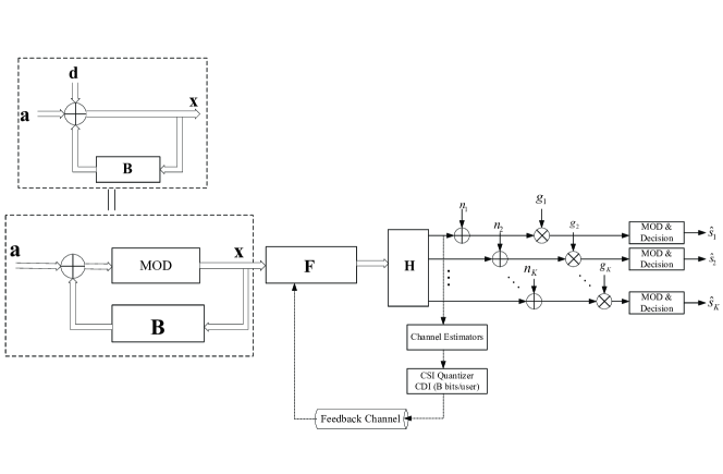
Figure 1: TH precoding for multiuser MIMO downlink with quantized CSI feedback.

II System Model

As shown in Fig. 1, we consider the multi-user downlink systems where TH precoding [15] is used at the transmitter for multi-user interference pre-subtraction. The transmitter is equipped with $n_{T}$ transmit antennas and $K$ decentralized users each has a single antenna such that $K\leq n_{T}$. Let the vector $\mathbf{s}=[s_{1},\cdots,s_{K}]^{T}\in\mathbb{C}^{K\times 1}$ represent the modulated signal vector for all users, where $s_{k}$ is the $k$-th modulated symbol stream for user $k$. Here we assume that an $M$-ary square constellation ($M$ is a square number) is employed in each of the parallel data streams and the constellation set is $\mathcal{A}=\big{\{}s_{I}+js_{Q}|~{}s_{I},s_{Q}\in\pm 1\sqrt{\frac{3}{2(M-1)}},\pm 3\sqrt{\frac{3}{2(M-1)}},\cdots,\pm\sqrt{M}\sqrt{\frac{3}{2(M-1)}}\big{\}}$. In general, the average transmit symbol energy is normalized, i.e. $\mathbb{E}\{|s_{k}|^{2}\}=1$. $\mathbf{s}$ is fed to the precoding unit, which consists of a backward square matrix $\mathbf{B}$ and a nonlinear operator $\text{MOD}_{\tau}(\cdot)$ which acts independently over the real and imaginary parts of its input as follows

$$\text{MOD}_{\tau}(x)=x-\tau\bigg{\lfloor}\frac{x+\tau}{2\tau}\bigg{\rfloor},$$ (1)

where $\tau=\sqrt{M}\sqrt{\frac{3}{2(M-1)}}$, $\lfloor z\rfloor$ is the largest integer not exceeding $z$. $\mathbf{B}$ must be strictly lower triangular to allow data precoding in a recursive fashion [1]. The construction of $\mathbf{B}$ will depend on the level of CSI of the supported users available at the transmitter side. If we temporarily neglect the nonlinear operator $\text{MOD}_{\tau}(\cdot)$ in Fig. 1, the channel signal vector $\mathbf{x}=[x_{1},\cdots,x_{K}]^{T}$ can be generated as

$$x_{1} =s_{1},$$

$$x_{k} =s_{k}-\sum_{l=1}^{k-1}[\mathbf{B}]_{k,l}x_{l},~{}k=2,\cdots,K.$$ (2)

In this way, if $\mathbf{b}=\left(\mathbf{I}+\mathbf{B}\right)^{-1}\mathbf{s}$ become large in the presence of deep fading the transmit power can be greatly increased. TH precoding modulo (1) reduces the transmit symbols into the boundary square region of $\mathcal{R}=\{x+jy|x,y\in(-\tau,\tau)\}$. With (1) and (II) the channel signals are equivalently given as

$$x_{k}=s_{k}+d_{k}-\sum_{l=1}^{k-1}[\mathbf{B}]_{k,l}x_{l},~{}k=2,\cdots,K,$$ (3)

where $d_{k}\in\left\{2\tau(p_{I}+jp_{Q})|~{}p_{I},p_{Q}\in\mathbb{Z}\right\}$ is properly selected to ensure the real and imaginary parts of $x_{k}$ are constrained into $\mathcal{R}$ [1]. The constellation of the modified data symbols $v_{k}=s_{k}+d_{k}$ is simply the periodic extension of the original constellation along the real and imaginary axes. Equivalently, the effective data symbols $v_{k}$ ($k=2,\cdots,K$) are passed into $\mathbf{B}$, which is implemented by the feedback structure. Thus, we have

$$\mathbf{v}=\mathbf{C}\mathbf{x},$$ (4)

where $\mathbf{v}=[v_{1},v_{2},\cdots,v_{K}]^{T}$ and

$$\mathbf{C}=\mathbf{B}+\mathbf{I}.$$ (5)

We will make the standard observation that the elements of $\mathbf{x}$ are almost uncorrelated and uniformly distributed over the Voronoi region of the constellation $\mathcal{R}$, and that such a model becomes more precise as $n_{T}$ increases [11, Theorem 3.1]. With $\mathbb{E}\left\{\mathbf{s}\mathbf{s}^{H}\right\}=\mathbf{I}$, the covariance of $\mathbf{x}$ can be accurately approximated as $\mathbf{R_{x}}=\frac{M}{M-1}\mathbf{I}$[11]. Moreover, the induced shaping loss by the non-Gaussian signaling leads to the fact that the achievable rate can be up to $1.53$ dB from the channel capacity [21]. However, as indicated in [1], the so-called shaping loss can be bridged by higher-dimensional precoding lattices. A scheme named “inflated lattice” precoding has been proved to be capacity-achieving in [22]. Thus, following [1], we will ignore the shaping gap in this work.

A spatial channel pre-equalization is performed at the transmitter side using a feedforward precoding matrix $\mathbf{F}\in\mathbb{C}^{n_{T}\times K}$. Throughout this work, we assume equal power allocation to all supported users. Then the received signal can be written as

$$\mathbf{r}=\sqrt{\frac{P}{\kappa}}\mathbf{H}\mathbf{F}\mathbf{x}+\mathbf{n},$$ (6)

where $\mathbf{H}=\left[\mathbf{h}_{1}^{T},\cdots,\mathbf{h}_{K}^{T}\right]^{T}$ is the compact flat fading channel matrix consisting of all users’s channel vectors and $\mathbf{h}_{k}\in\mathbb{C}^{n_{T}\times 1}$ is the channel from the transmitter to user $k$. $\kappa$ is used for transmit power normalization. $\mathbf{F}\in\mathbb{C}^{n_{T}\times K}$ satisfies transmit power constraint $\frac{P}{\kappa}\text{Tr}\{\mathbf{F}\mathbf{R}_{\mathbf{x}}\mathbf{F}^{H}\}=\frac{P}{\kappa}\frac{M}{M-1}\text{Tr}\{\mathbf{F}\mathbf{F}^{H}\}=P$. As for $\mathbf{B}$, $\mathbf{F}$ is also designed based on the level of CSI available to the transmitter. We assume $\mathbf{n}$ is the white additive noise at all the receivers with the covariance $\mathbf{R}_{\mathbf{n}}=\mathbf{I}$ without loss of generality. Each receiver compensates for the channel gain by dividing by a factor $g_{k}$ prior to the modulo operation as follows:

$$\mathbf{y} =\mathbf{G}\left(\sqrt{\frac{P}{\kappa}}\mathbf{H}\mathbf{F}\mathbf{x}+\mathbf{n}\right),$$ (7)

where $\mathbf{G}=\text{diag}\left(g_{1,1},\cdots,g_{K,K}\right)$.

Throughout this work, we assume each receiver can obtain perfect CSI of his own through channel estimation and feeds back this information to the transmitter via a zero-delay feedback link with possible rate-constraints. In this part, we assume this feedback information is perfect at the transmitter. The design of TH precoding for MU MIMO systems with perfect CSI has been studied in [1] where, for simplicity, the authors restrict the work to the systems with equal number of transmit antennas and users. In this part, we review and extend that construction for systems with arbitrary number of users no more that of the transmit antennas.

With perfect CSI at the transmitter, let the QR decomposition of the compact channels be $\mathbf{H}=\mathbf{RQ}$, where $\mathbf{R}=\left[r_{i,j}\right]\in\mathbb{C}^{K\times K}$ is a lower left triangular matrix and $\mathbf{Q}\in\mathbb{C}^{K\times n_{T}}$ is a semi-unitary matrix with orthonormal rows which satisfies $\mathbf{Q}\mathbf{Q}^{H}=\mathbf{I}$. Then the precoding matrix $\mathbf{F}$ is given as $\mathbf{F}=\mathbf{Q}^{H}$, the scaling matrix $\mathbf{G}$ is given as $\mathbf{G}=\sqrt{\frac{\kappa}{P}}\mathbf{\Delta}$ with $\mathbf{\Delta}=\text{diag}\left(r_{1,1}^{-1},\cdots,r_{K,K}^{-1}\right)$ and the feedback matrix reads $\mathbf{B}=\mathbf{\Delta HF}-\mathbf{I}=\mathbf{\Delta R}-\mathbf{I}$. According to the transmit power constraint $\frac{P}{\kappa}\frac{M}{M-1}K=P$, we have $\kappa=\frac{M}{M-1}K$. With the processing, the effective received data symbols $\mathbf{y}$ corrupted by additive noise can be written as[1]

$$\mathbf{y}=\mathbf{v}+\mathbf{G}\mathbf{n}.$$ (8)

At the receivers, each symbol in $\mathbf{y}$ is firstly modulo reduced into the boundary region of the signal constellation $\mathcal{A}$. A quantizer of the original constellation will follow the modulo operation to detect the received signals. The SNR $\xi_{k}$ for receiver $k$ can be written as

$$\xi_{k}=\frac{P}{\kappa}|r_{k,k}|^{2}.$$ (9)

In the following part, we will describe how to implement the precoding with quantized CSI obtained at the transmitter.

III System with Quantized transmit CSI

In practical systems, perfect CSI is never available at the transmitter. For example, in a FDD system, the transmitter obtains CSI for the downlink through the limited feedback of $B$ bits by each receiver. Following the studies of quantized CSI feedback in [2, 19], channel direction vector is quantized at each receiver, and the corresponding index is fed back to the transmitter via an error and delay-free feedback channel. Given the quantization codebook $\mathbb{W}=\{\mathbf{w}_{1},\cdots,\mathbf{w}_{n}\}$ ($\mathbf{w}_{i}\in\mathbb{C}^{1\times n_{T}}$), which is known to both the transmitter and all the receivers, the $k$-th receiver selects the quantized channel direction vector of its own channel as follows:

$${\hat{\mathbf{h}}_{k}}=\text{arg}\max_{\mathbf{w}_{i}\in\mathbb{W}}\{|\bar{{\mathbf{h}}}_{k}\mathbf{w}_{i}|^{2}\},$$ (10)

where $\bar{{\mathbf{h}}}_{k}=\frac{\mathbf{h}_{k}}{\|\mathbf{h}_{k}\|}$ is the channel direction vector of user $k$.

In this work, we use RVQ codebook, in which the $n$ quantization vectors are independently and isotropically distributed on the $n_{T}$–dimensional complex unit sphere. Although RVQ is suboptimal for a finite-size system, it is very amenable to analysis and also its performance is close to the optimal quantization[2]. Using the result in [2], for user $k$ we have

$$\bar{\mathbf{h}}_{k}=\hat{\mathbf{h}}_{k}\cos\theta_{k}+\tilde{\mathbf{h}}_{k}\sin\theta_{k},$$ (11)

where $\cos^{2}\theta_{k}=|\bar{\mathbf{h}}_{k}\hat{\mathbf{h}}_{k}^{H}|^{2}$, $\tilde{\mathbf{h}}_{k}\in\mathbb{C}^{1\times n_{T}}$ is a unit norm vector isotropically distributed in the orthogonal complement subspace of $\hat{\mathbf{h}}_{k}$ and independent of $\sin\theta_{k}$. Then $\mathbf{H}$ can be written as

$$\mathbf{H}=\mathbf{\Gamma}\left(\mathbf{\Phi}\hat{\mathbf{H}}+\mathbf{\Omega}\tilde{\mathbf{H}}\right),$$ (12)

where $\mathbf{\Gamma}=\text{diag}\big{(}\rho_{1},\cdots,\rho_{K}\big{)}$ with $\rho_{k}=\|\mathbf{h}_{k}\|$, $\mathbf{\Phi}=\text{diag}\left(\cos\theta_{1},\cdots,\cos\theta_{K}\right)$ and $\mathbf{\Omega}=\text{diag}\big{(}\sin\theta_{1},\\ \cdots,\sin\theta_{K}\big{)}$, $\hat{\mathbf{H}}=\left[\hat{\mathbf{h}}_{1}^{T},\cdots,\hat{\mathbf{h}}_{K}^{T}\right]^{T}$ and $\tilde{\mathbf{H}}=\left[\tilde{\mathbf{h}}_{1}^{T},\cdots,\tilde{\mathbf{h}}_{K}^{T}\right]^{T}$. For simplicity of analysis, in this work we consider the quantization cell approximation used in [23, 19], where each quantization cell is assumed to be a Voronoi region of a spherical cap with surface area approximately equal to $\frac{1}{n}$ of the total surface area of the $n_{T}$-dimensional unit sphere. For a given codebook $\mathbb{W}$, the actual quantization cell for vector $\mathbf{w}_{i}$, $\mathcal{R}_{i}=\left\{\bar{\mathbf{h}}:|\bar{\mathbf{h}}\mathbf{w}_{i}|^{2}\geq|\bar{\mathbf{h}}\mathbf{w}_{j}|^{2},\forall~{}i\neq j\right\}$, is approximated as $\tilde{\mathcal{R}}_{i}\approx\left\{\bar{\mathbf{h}}:|\bar{\mathbf{h}}\mathbf{w}_{i}|\geq 1-\delta\right\}$, where $\delta=2^{-\frac{B}{n_{T}-1}}$.

With the quantized CDI at the transmitter side, the transmitter obtains the feedforward precoding matrix $\mathbf{F}$ and feedback matrix $\mathbf{B}$ through the QR decomposition of compact channel matrix $\hat{\mathbf{H}}$ in the same way as the QR decomposition of matrix $\mathbf{H}$, i.e. $\hat{\mathbf{H}}=\hat{\mathbf{R}}\hat{\mathbf{Q}}$, where the matrices $\hat{\mathbf{R}}$ and $\hat{\mathbf{Q}}$ have the same structure as the matrices $\mathbf{R}$ and $\mathbf{Q}$ respectively. Then we have $\mathbf{F}=\hat{\mathbf{Q}}^{H}$ and $\mathbf{B}=\left(\text{diag}\left\{\hat{\mathbf{R}}\right\}\right)^{-1}\hat{\mathbf{R}}-\mathbf{I}$. In addition, the scaling matrix at the receivers now becomes

$$\mathbf{G}=\sqrt{\frac{\kappa}{P}}\left(\mathbf{\Gamma}\mathbf{\Phi}~{}\text{diag}\left\{\hat{\mathbf{R}}\right\}\right)^{-1}.$$ (13)

Using the same operation at the receiver side as that in perfect CSI case to detect the received signals, the detected signal vector $\hat{\mathbf{y}}$ can be further written as

$$\hat{\mathbf{y}} =\mathbf{G}\left(\sqrt{\frac{P}{\kappa}}\mathbf{H}\mathbf{F}\mathbf{x}+\mathbf{n}\right)$$

$$=\mathbf{G}\sqrt{\frac{P}{\kappa}}\mathbf{\Gamma}\left(\mathbf{\Phi}\hat{\mathbf{H}}+\mathbf{\Omega}\tilde{\mathbf{H}}\right)\mathbf{F}\mathbf{x}+\mathbf{G}\mathbf{n}$$

$$=\mathbf{v}+\left(\mathbf{\Phi}~{}\text{diag}\left\{\hat{\mathbf{R}}\right\}\right)^{-1}\mathbf{\Omega}\tilde{\mathbf{H}}\hat{\mathbf{Q}}^{H}\mathbf{x}+\sqrt{\frac{\kappa}{P}}\left(\mathbf{\Gamma}\mathbf{\Phi}~{}\text{diag}\left\{\hat{\mathbf{R}}\right\}\right)^{-1}\mathbf{n},$$ (14)

where we have used the relationship $\mathbf{v}=\left(\text{diag}\left\{\hat{\mathbf{R}}\right\}\right)^{-1}\hat{\mathbf{R}}\mathbf{x}$. In (III), the first term is the useful signal vector for all the users and the second term is interference signal caused by the quantized CSI.

According to (III), the output signal-to-interference-plus-noise ratio (SINR) $\gamma_{k}$ for receiver $k$ can be written as

$$\gamma_{k} =\frac{1}{\frac{\sin^{2}\theta_{k}}{|\hat{r}_{k,k}|^{2}\cos^{2}\theta_{k}}\|\tilde{\mathbf{h}}_{k}\hat{\mathbf{Q}}^{H}\|^{2}+\frac{\kappa}{P}\frac{1}{\rho_{k}^{2}|\hat{r}_{k,k}|^{2}\cos^{2}\theta_{k}}}$$

$$=\frac{\frac{P}{\kappa}\rho_{k}^{2}|\hat{r}_{k,k}|^{2}\cos^{2}\theta_{k}}{\frac{P}{\kappa}\rho_{k}^{2}\|\tilde{\mathbf{h}}_{k}\hat{\mathbf{Q}}^{H}\|^{2}\sin^{2}\theta_{k}+1}.$$ (15)

IV Average Sum Rate Analysis under Quantized CSI Feedback

In this section we will study the achievable average sum rate of the proposed quantized CSI feedback TH precoding scheme. Although the exact distribution of each term in the expression of the output SINR $\gamma_{k}$ in $(15)$ can be obtained (see for the detailed information), these terms are located at both the numerator and the denominator in $(15)$. Thus, to obtain the exact closed-form expression of the distribution of output SINR $\gamma_{k}$ can be very difficult if not impossible, not to mention the exact closed-form expression of the average sum rate. Thus, to simplify analysis, we have appealed to studying some bounds of the average sum rate and the average sum rate loss instead of exact results. For tractability, throughout this section we assume each user’s channel is Rayleigh-faded. In the following subsection, we will first study the statistical distribution of the power of interference signal at each user caused by quantized CSI.

IV-A Interference Part

In this subsection, assuming Rayleigh fading channel and RVQ for quantized CSI feedback, we will derive the statistical distribution of interference part $\frac{P}{\kappa}\rho_{k}^{2}\|\tilde{\mathbf{h}}_{k}\hat{\mathbf{Q}}^{H}\|^{2}\sin^{2}\theta_{k}$ in (III). It is well known that $\rho_{k}^{2}$ has a $\chi_{2n_{T}}^{2}$ distribution and the distribution of $\sin^{2}\theta_{k}$ is given in [18, 2]. However, since $\tilde{\mathbf{h}}_{k}\perp\hat{\mathbf{h}}_{k}$ ($k=1,\cdots,K$) and $\hat{\mathbf{Q}}$ is determined by $\hat{\mathbf{h}}_{k}$ ($k=1,\cdots,K$), $\tilde{\mathbf{h}}_{k}$ for $k=1,\cdots,K$ are not independent of $\hat{\mathbf{Q}}$. The distribution of the term $\|\tilde{\mathbf{h}}_{k}\hat{\mathbf{Q}}^{H}\|^{2}$ is still unknown and to obtain the exact result is not trivial. The following lemma presents the exact distribution of this interference term. It is one of the key contributions of this paper.

Lemma 1

For $1<K<n_{T}$, the random variables $\varepsilon_{k}=\|\tilde{\mathbf{h}}_{k}\hat{\mathbf{Q}}^{H}\|^{2}$ for $k=1,\cdots,K$ follow the same beta distribution with shape $(K-1)$ and $(n_{T}-K)$ which is denoted as $\varepsilon_{k}\sim\mathrm{Beta}(K-1,n_{T}-K)$. In addition, the probability density function (p.d.f.) of $\varepsilon_{k}$ is given as

$$f_{\varepsilon_{k}}(x)=\frac{1}{\beta(K-1,n_{T}-K)}x^{K-2}(1-x)^{n_{T}-K-1}.$$ (16)

where $\beta(a,b)=\int_{0}^{1}t^{a-1}t^{b-1}{\rm d}t$ is beta function [24]. Specially, when $K=1$ there is no interference term. When $K=n_{T}$, $\varepsilon_{k}=\|\tilde{\mathbf{h}}_{k}\hat{\mathbf{Q}}^{H}\|^{2}$ is equal to $1$ which is a constant.

Proof:

See Appendix A. ∎

Lemma 1 implies a very interesting result that, with randomly ordered user channel vectors, the signal of the user which is precoded ahead suffers from the same interference signal power as the signals of the users which are precoded afterwards. In the following we will only focus on the general situation that $1<K<n_{T}$. However, it is easy to check that all the obtained results also apply to the special cases of $K=1$ and $K=n_{T}$.

The expectation of the logarithm of the interference term $\varepsilon_{k}$, which is shown to be useful in the following theorems, is obtained in the following lemma.

Lemma 2

The expectation of the logarithm of the interference term $\varepsilon_{k}$ is given by

$$\mathbb{E}_{\mathbf{H},\mathbb{W}}\left[-\log_{2}\left(\|\tilde{\mathbf{h}}_{k}\hat{\mathbf{Q}}^{H}\|^{2}\right)\right]=\log_{2}e\sum_{m=K-1}^{n_{T}-2}\sum_{l=0}^{n_{T}-m-2}\frac{(n_{T}-2)!}{m!~{}l!~{}(n_{T}-m-2-l)!}(-1)^{l}\frac{1}{m+l}$$ (17)

Proof:

See Appendix B. ∎

IV-B Upper Bounds on the Average Sum Rate Loss and Sum Rate

The instantaneous achievable rates for user $k$ with perfect CSI and quantized CSI feedback are given as

$$R_{P,k}=\log_{2}\left(1+\xi_{k}\right)$$ (18)

and

$$R_{Q,k}=\log_{2}(1+\gamma_{k}),$$ (19)

respectively. The following theorem quantifies the average sum rate performance degradation as a function of the feedback rate.

Theorem 1

With $B$ feedback bits per user, the average sum rate loss of user $k$ due to quantized CSI feedback can be upper bounded by

$$\Delta R_{k} =\mathbb{E}_{\mathbf{H},\mathbb{W}}\{R_{P,k}-R_{Q,k}\}$$

$$\leq\Delta R=\log_{2}\left(1+cP~{}2^{-\frac{B}{n_{T}-1}}\right)+\frac{\log_{2}(e)}{n_{T}-1}\sum_{i=1}^{n_{T}-1}\beta\left(n,\frac{i}{n_{T}-1}\right),$$ (20)

where $c=\frac{(K-1)n_{T}}{\kappa(n_{T}-1)}$ and $n=2^{B}$ is the size of codebook.

Proof:

See Appendix C. ∎

According to the results in [2, Theorem 1], the average sum rate loss due to quantized feeback for ZF precoding is upper bounded by $\Delta R_{zf}<\log_{2}\left(1+P~{}2^{-\frac{B}{n_{T}-1}}\right)$. We find the first term at the right hand side (RHS) of (1) can be approximated as $\log_{2}\left(1+P~{}2^{-\frac{B}{n_{T}-1}}\right)$ with high order constellation, large number of transmit antennas and large number of supported users. Thus, the second term at the RHS of (1) can be seen as the sum rate degradation of nonlinear precoding compared with that of linear precoding when only quantized CSI is available at the transmitter side. In addition, similar to the results for the linear ZF beamforming in [2], the rate loss for nonlinear precoding is also an increasing function of the system SNR ($P$). Thus, the system with fixed feedback rate is interference-limited at high SNR regime, which is shown in the following theorem.

Theorem 2

The average sum rate of user $k$ achieved by quantized CSI-based TH precoding with $B$ feedback bits per user is bounded as

$$R_{Q,k}\leq\log_{2}e\left(\sum_{m=K-1}^{n_{T}-2}\sum_{l=0}^{n_{T}-m-2}\frac{(n_{T}-2)!}{m!~{}l!~{}(n_{T}-m-2-l)!}(-1)^{l}\frac{1}{m+l}+\frac{1}{n_{T}-1}\sum_{l=1}^{n}\frac{1}{l}\right),$$ (21)

where $n=2^{B}$ is the size of codebook.

Proof:

See Appendix D. ∎

We can see from this theorem that, with fixed feedback bits per user, as the interference and signal power both increase linearly with $P$, the system becomes interference-limited and the average sum rate converges to an upper bound. These can also be observed from the simulation results in Fig. 3.

In the context of linear ZF precoding in [2], the author showed the interference-limited scenario can be avoided by scaling the feedback rate linearly with the SNR $P_{\text{dB}}$ (in decibels). Particularly, it is showed in [2, Theorem 3] that in order to maintain a constant average sum rate loss no greater than $\log_{2}b$ bits per user between the system with perfect CSI and the system with finite-rate feedback, it is sufficient to scale the number of feedback bits per user according to

$$B=(n_{T}-1)\frac{\log_{2}10}{10}P_{\text{dB}}-(n_{T}-1)\log_{2}(b-1).$$ (22)

However, for nonlinear TH precoding, the explicit relationship between the feedback rate and the SNR to maintain a constant average sum rate loss cannot be easily obtained. This is mainly due to the fact that the expression of average sum rate loss in (1) is a much more complex function of $n$ ($B$) than the corresponding expression for linear ZF precoding given in [2, Theorem 1]. In the following we will derive a corresponding relationship for the system employing TH precoding. First, in Appendix E we show that the second term at the RHS of (1) can be bounded by a decreasing function of $n$ for a fixed $n_{T}$. In addition, this upper bound approaches zero as $n\rightarrow\infty$. Thus, as $n$ scales linearly with SNR (in decibels), for an arbitrary given constant $0<\varepsilon<1$, we can always find a positive integer $N(\varepsilon)$ such that, whenever $n\geq N(\varepsilon)$,

$$\Delta R\leq\log_{2}\left(1+cP~{}2^{-\frac{B}{n_{T}-1}}\right)+\varepsilon.$$ (23)

To characterize a sufficient condition of the scaling of feedback rate, we set the RHS of (23) to be the maximum allowable gap of $\log_{2}b$. After some simple manipulations, we get

$$B =(n_{T}-1)\log_{2}P-\log_{2}(b-2^{\varepsilon}-1)+\log_{2}c$$

$$=(n_{T}-1)\frac{\log_{2}10}{10}P_{\text{dB}}-\log_{2}(b-2^{\varepsilon}-1)+\log_{2}c.$$ (24)

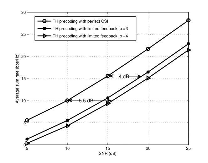
Figure 2: $4\times 4$ system with increasing number of feedback bits.

In Fig. 2, the average sum rate curves are shown for a system with $n_{T}=4$ and $K=4$. The feedback rate is assumed to scale according to the relationship given in (IV-B). Notice that, since $\varepsilon$ can be set to be a small number when $B$ is large enough, in the simulation we set $\varepsilon=0$ to get a stronger condition than (IV-B). Quantized CSI-based TH precoding is seen to perform within around $4$ dB and $5.5$ dB of TH precoding with perfect CSI for $b=3$ and $b=4$ respectively.

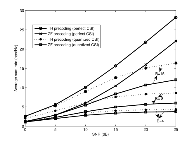
Figure 3: The average sum rate performance of TH precoding and ZF precoding for both perfect CSI and quantized CSI.

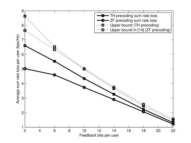
Figure 4: The average sum rate loss per user and corresponding upper bounds against the number of feedback bits. $P=25$ dB.

V Numerical Results

In this section we present some numerical results. We assume $n_{T}=K=4$. Here the SNR of the systems is defined to be equal to $P$.

Fig. 3 shows the average sum rate performance of TH precoding and linear ZF precoding with both perfect CSI and quantized CSI, and $4,8$ and $15$ feedback bits per user. We can see TH precoding performs better than linear precoding in both perfect CSI and quantized CSI cases. When the SNR is small and moderate, the average sum rate achieved by quantized CSI-based TH precoding can even be better than that of perfect CSI-based linear ZF precoding.

Fig. 4 plots the average sum rate loss per user as a function of the number of feedback bits for both ZF precoding and TH precoding in a system at an SNR of $25$ dB. We also plot the upper bound from Theorem 1 in this paper and the upper bound from Theorem $1$ in [2]. From the figure we can see that nonlinear precoding suffers from imperfect CSI more than linear precoding does. However, the performance of nonlinear precoding can still be better than linear precoding when SNR is not large or the feedback quantization resolution is high enough. In addition, we notice that the upper bound for TH precoding tracks the true rate loss quite closely, and appears to converge faster than the upper bound for linear precoding obtained in [2] as $B$ increases.

VI Conclusion

In this paper, we have investigated the implementation of TH precoding in the downlink multiuser MIMO systems with quantized CSI at the transmitter side. In particular, our scheme generalized the results in [1] to more general system setting where the number of users $K$ in the systems can be less than or equal to the number of transmit antennas $n_{T}$. In addition, we studied the achievable average sum rate of the proposed scheme by deriving expressions of upper bounds on both the average sum rate and the mean loss in sum rate due to CSI quantization. Our numerical results showed that the nonlinear TH precoding could achieve much better performance than that of linear zero-forcing precoding for both perfect CSI and quantized CSI cases. In addition, our derived upper bound for TH precoding converged to the true rate loss faster than the upper bound for zero-forcing precoding obtained in [2] as the number of feedback bits increased.

Appendix A Proof of Lemma 1

The results for the special cases that $K=1$ and $n_{T}$ are trivial. In the following we will consider the cases that $1<K<n_{T}$. Since the user channel vectors in $\mathbf{H}$ are unordered, so are the quantized channel direction vectors in $\hat{\mathbf{H}}=\left[\hat{\mathbf{h}}_{1}^{T},\cdots,\hat{\mathbf{h}}_{K}^{T}\right]^{T}$. According to the QR decomposition of $\hat{\mathbf{H}}$ we have

$$\hat{\mathbf{h}}_{k}=\sum_{l=1}^{k}\hat{r}_{k,l}\hat{\mathbf{q}}_{l},$$ (25)

If we require $\hat{r}_{i,i}>0$ for $i=1,\cdots,K$, this decomposition is unique. Particularly, we have $\hat{r}_{1,1}=1$ and $\hat{\mathbf{q}}_{1}=\hat{\mathbf{h}}_{1}$. In addition, $\tilde{\mathbf{h}}_{k}$ is isotropically distributed in the null space of $\hat{\mathbf{h}}_{k}$[2]. Thus, for $k=1$ we have $\tilde{\mathbf{h}}_{1}\bot~{}\hat{\mathbf{q}}_{1}$ or equivalently $\tilde{\mathbf{h}}_{1}$ is an isotropically distributed unit vector in the null space of $\hat{\mathbf{q}}_{1}$.

With the assumption of RVQ, the quantized channel direction vectors $\hat{\mathbf{h}}_{k}(k=1,\cdots,K)$ are independently and isotropically distributed on the $n_{T}$–dimensional complex unit sphere due to the assumption of i.i.d. Rayleigh fading. Thus we can conclude that the orthonormal basis $\hat{\mathbf{q}}_{1},\cdots,\hat{\mathbf{q}}_{K}$ of the subspace spanned by quantized channel vectors $\hat{\mathbf{h}}_{k}(k=1,\cdots,K)$ have no preference of direction, i.e., $\left[\hat{\mathbf{q}}_{1}^{T},\cdots,\hat{\mathbf{q}}_{K}^{T}\right]^{T}$ is isotropically distributed in the $K\times n_{T}$ semi-unitary space. Thus, to derive the distribution of $\varepsilon_{1}=\|\tilde{\mathbf{h}}_{1}\hat{\mathbf{Q}}^{H}\|^{2}$, we can assume $\hat{\mathbf{q}}_{i}=\mathbf{e}_{i}$ for $i=1,\cdots,K$ without loss of generality, where $\mathbf{e}_{i}$ is the $i$-th row of the identity matrix $\mathbf{I}_{n_{T}}$. Recall that $\tilde{{\mathbf{h}}}_{1}\bot\hat{\mathbf{q}}_{1}$, thus the random vector $\tilde{{\mathbf{h}}}_{1}$ can be written in the form of $\tilde{{\mathbf{h}}}_{1}=[0,\mathbf{v}]$, where the vector $\mathbf{v}=[v_{1},v_{2},\cdots,v_{n_{T}-1}]$ is isotropically distributed on the $\left(n_{T}-1\right)$–dimensional complex unit sphere. Then $\varepsilon_{1}=\|\tilde{\mathbf{h}}_{1}\hat{\mathbf{Q}}^{H}\|^{2}=\sum_{l=1}^{K-1}|v_{l}|^{2}$. Let $t_{l}=|v_{l}|^{2}$. It has been obtained in [25] that the joint p.d.f. of $t_{1},\cdots,t_{K-1}$ is

$$f(t_{1},\ldots,t_{K-1})=\left\{\begin{array}[]{ll}\frac{\Gamma(n_{T}-1)}{\Gamma(n_{T}-K)}\left(1-\sum_{i=1}^{K-1}t_{i}\right)^{n_{T}-K-1},&t_{i}\geq 0~{}\text{for}~{}i=1,\cdots,K-1,\sum_{i=1}^{K-1}t_{i}=1\\ 0,&\text{otherwise}\end{array}\right..$$ (28)

Now we want to obtain the distribution of $u_{1}=\sum_{l=1}^{K-1}t_{l}$. We define the following transformation of variables

$$u_{1}=\sum_{l=1}^{K-1}t_{l},~{}~{}u_{i}=t_{i}~{}~{}~{}\text{for}~{}i=2,\cdots,K-1.$$

It is easy to obtain the corresponding Jacobian is $J=1$. Thus the joint p.d.f. of $u_{1},\cdots,u_{K-1}$ is

$$f_{u_{1},\ldots,u_{K-1}}\left(x_{1},\cdots,x_{K-1}\right)=\frac{\Gamma(n_{T}-1)}{\Gamma(n_{T}-K)}\left(1-x_{1}\right)^{n_{T}-K-1}.$$ (29)

Since $0\leq t_{i}\leq 1$, we have $0\leq t_{1}=u_{1}-\sum_{i=2}^{K-1}u_{i}\leq 1$. The region of the random variables after transformation can be obtained as $\mathcal{D}=\big{\{}\left(u_{1},\cdots,u_{K-1}\right)~{}|~{}0\leq\sum_{l=2}^{K-1}u_{l}\leq u_{1}\leq 1,0\leq u_{i}\leq 1~{}\text{for}~{}i=2,\cdots,K-1\big{\}}$. Then the marginal distribution of $u_{1}$ can be obtained as

$$f_{u_{1}}(x) =\int\cdots\int_{\mathcal{D}}f(x,x_{2}\ldots,x_{K-1})~{}{\rm d}x_{2}\cdots{\rm d}x_{K-1}$$

$$=\int\cdots\int_{\mathcal{D}}\frac{\Gamma(n_{T}-1)}{\Gamma(n_{T}-K)}\left(1-x_{1}\right)^{n_{T}-K-1}~{}{\rm d}x_{2}\cdots{\rm d}x_{K-1}$$

$$\mathop{=}\limits^{(a)}\frac{\Gamma(n_{T}-1)}{\Gamma(n_{T}-K)}(1-x)^{n_{T}-K-1}\frac{x^{K-2}}{\left(K-2\right)!}$$

which is given by (16), where in (a) we have used the identity $\mathop{\int\int{\cdots\int{}}}\limits_{\scriptstyle\sum_{i=1}^{n}t_{i}\leq h\hfill\atop\scriptstyle t_{1}\geq 0,\cdots,t_{n}\geq 0\hfill}~{}{\rm d}t_{1}\cdots~{}{\rm d}t_{n}=\frac{h^{n}}{n!}$ [24]. We find that $\varepsilon_{1}=u_{1}$ follows beta distribution with shape $(K-1)$ and $(n_{T}-K)$. In the following we will prove $\varepsilon_{k}$s have the same distribution.

Let $\bm{\pi}$ be an arbitrary and channel-independent permutation of $(1,2,\cdots,K)$. $\mathbf{P}_{\bm{\pi}}=\big{[}\mathbf{1}_{\bm{\pi}(1)},\cdots,\\ \mathbf{1}_{\bm{\pi}(K)}\big{]}^{T}$ is the permutation matrix corresponding to $\bm{\pi}$ and $\mathbf{1}_{\bm{\pi}(i)}$ is the $\bm{\pi}(i)$-th column of identity matrix. We denote $\hat{\mathbf{H}}_{\bm{\pi}}=\mathbf{P}_{\bm{\pi}}\hat{\mathbf{H}}=\left[\mathbf{h}_{\bm{\pi}(1)}^{T},\cdots,\mathbf{h}_{\bm{\pi}(K)}^{T}\right]^{T}$ the matrix obtained by permutating the row vector of matrix $\hat{\mathbf{H}}$ according to the permutation $\bm{\pi}$. Then the QR decomposition of $\hat{\mathbf{H}}_{\bm{\pi}}$ can be written as $\hat{\mathbf{H}}_{\bm{\pi}}=\mathbf{P}_{\bm{\pi}}\hat{\mathbf{R}}\hat{\mathbf{Q}}=\hat{\mathbf{R}}_{\bm{\pi}}\hat{\mathbf{Q}}_{\bm{\pi}}$. With the assumption that $\hat{\mathbf{R}}_{\bm{\pi}}$ has positive diagonal elements, the above QR decomposition of $\hat{\mathbf{H}}_{\bm{\pi}}$ is unique. Using Givens transformation, there is a series of Givens matrices $\mathbf{G}_{1},\cdots,\mathbf{G}_{K-1}\in\mathbb{C}^{K\times K}$ which satisfy $\mathbf{P}_{\bm{\pi}}\hat{\mathbf{R}}\mathbf{G}_{1}\cdots\mathbf{G}_{K-1}=\bar{\mathbf{R}}_{\bm{\pi}}$ [26], where $\bar{\mathbf{R}}_{\bm{\pi}}\in\mathbb{C}^{K\times K}$ is a lower triangular matrix with positive diagonal elements. Since Givens matrix is unitary, we have $\mathbf{G}_{1}\cdots\mathbf{G}_{K-1}\mathbf{G}_{K-1}^{H}\cdots\mathbf{G}_{1}^{H}=\mathbf{I}$. So $\hat{\mathbf{H}}_{\bm{\pi}}$ can be written as $\hat{\mathbf{H}}_{\bm{\pi}}=\bar{\mathbf{R}}_{\bm{\pi}}\mathbf{G}_{K-1}^{H}\cdots\mathbf{G}_{1}^{H}\hat{\mathbf{Q}}$. Let $\bar{{\mathbf{Q}}}_{\bm{\pi}}=\mathbf{G}_{K-1}^{H}\cdots\mathbf{G}_{1}^{H}\hat{\mathbf{Q}}$. Then we have $\hat{\mathbf{H}}_{\bm{\pi}}=\bar{\mathbf{R}}_{\bm{\pi}}\bar{\mathbf{Q}}_{\bm{\pi}}$ where $\bar{{\mathbf{Q}}}_{\bm{\pi}}$ is unitary. Thus $\hat{\mathbf{H}}_{\bm{\pi}}=\bar{\mathbf{R}}_{\bm{\pi}}\bar{\mathbf{Q}}_{\bm{\pi}}$ is also a QR decomposition of $\hat{\mathbf{H}}_{\bm{\pi}}$. Using the uniqueness of QR decomposition, we conclude that $\bar{\mathbf{Q}}_{\bm{\pi}}=\hat{\mathbf{Q}}_{\bm{\pi}}$ and $\bar{\mathbf{R}}_{\bm{\pi}}=\hat{\mathbf{R}}_{\bm{\pi}}$. Thus we have

$$\varepsilon_{k} =\|\tilde{\mathbf{h}}_{k}\hat{\mathbf{Q}}^{H}\|^{2}$$

$$=\|\tilde{\mathbf{h}}_{k}\hat{\mathbf{Q}}_{\bm{\pi}}^{H}\mathbf{G}_{K-1}^{H}\cdots\mathbf{G}_{1}^{H}\|^{2}$$

$$\mathop{=}\limits^{(b)}\|\tilde{\mathbf{h}}_{k}\bar{\mathbf{Q}}_{\bm{\pi}}^{H}\|^{2},$$ (30)

where $(b)$ is due to the fact that the matrix $\mathbf{G}_{i}$ is unitary for $i=1,\cdots,K-1$. If we let $\bm{\pi}(1)=k$, $\hat{\mathbf{h}}_{k}$ will be the first row of $\hat{\mathbf{H}}_{\bm{\pi}}$. According to the previous derivation in the proof, we know $\varepsilon_{k}$ for $k=2,\cdots,K-1$ have the same distribution as $\varepsilon_{1}$ whose p.d.f. is give by (16).

Appendix B Proof of Lemma 2

Let $Y=\|\tilde{\mathbf{h}}_{k}\hat{\mathbf{Q}}^{H}\|^{2}$. As shown in Lemma 1, $Y$ follows the beta distribution with shape $(K-1)$ and $(n_{T}-K)$ and the cumulative distribution function (c.d.f.) is given by $\text{Pr}\left(Y\leq y\right)=I_{x}\left(K-1,n_{T}-K\right)$, where $I_{x}\left(\cdot,\cdot\right)$ is the regularized incomplete beta function. Using the facts that

$$I_{x}\left(a,b\right)=\sum_{m=a}^{a+b-1}\frac{(a+b-1)!}{m!(a+b-m-1)!}x^{m}(1-x)^{a+b-m-1},$$ (31)

$\mathbb{E}[X]=\int_{0}^{\infty}\text{Pr}\left(X\geq x\right){\rm d}x$ for nonnegative random variables and binomial expansion, we have

$$\mathbb{E}\left[-\ln Y\right] =\int_{0}^{\infty}\text{Pr}\left(Y\leq e^{-x}\right){\rm d}x$$

$$=\int_{0}^{\infty}I_{e^{-x}}(K-1,n_{T}-K){\rm d}x$$

$$=\int_{0}^{\infty}\left\{\sum_{m=K-1}^{n_{T}-2}\frac{(n_{T}-2)!}{m!(n_{T}-2-m)!}e^{-mx}(1-e^{-x})^{n_{T}-2-m}\right\}{\rm d}x$$

$$=\int_{0}^{\infty}\left\{\sum_{m=K-1}^{n_{T}-2}\frac{(n_{T}-2)!}{m!(n_{T}-2-m)!}e^{-mx}\sum_{l=0}^{n_{T}-m-2}\binom{n_{T}-m-2}{l}(-1)^{l}e^{-lx}\right\}{\rm d}x$$

$$=\sum_{m=K-1}^{n_{T}-2}\sum_{l=0}^{n_{T}-m-2}\frac{(n_{T}-2)!}{m!(n_{T}-2-m)!}\binom{n_{T}-m-2}{l}(-1)^{l}\frac{1}{m+l}$$

$$=\sum_{m=K-1}^{n_{T}-2}\sum_{l=0}^{n_{T}-m-2}\frac{(n_{T}-2)!}{m!~{}l!~{}(n_{T}-m-2-l)!}(-1)^{l}\frac{1}{m+l}.$$ (32)

Thus (17) is proved.

Appendix C Proof of Theorem 1

First we will prove the fact that $|r_{k,k}|^{2}$ and $\rho_{k}^{2}|\hat{r}_{k,k}|^{2}$ have the same distribution. Let the QR decomposition of matrix $\check{\mathbf{H}}=\mathbf{\Phi}\hat{\mathbf{H}}$ be $\check{\mathbf{Q}}\check{\mathbf{R}}$. It is easy to see $|\check{r}_{k,k}|^{2}=\rho_{k}^{2}|\hat{r}_{k,k}|^{2}$, where $\check{r}_{k,k}$ is the $k$-th diagonal element of $\check{\mathbf{R}}$. Since we assume using RVQ, $\check{\mathbf{H}}$ has the same distribution as $\mathbf{H}$. Thus $\rho_{k}^{2}|\hat{r}_{k,k}|^{2}$ has the same distribution as $|r_{k,k}|^{2}$.

Using (9), (III) (18) and (19), we can write

$$\Delta R_{k} =\mathbb{E}_{\mathbf{H},\mathbb{W}}\left\{\log_{2}\left(1+\frac{P}{\kappa}|r_{k,k}|^{2}\right)-\log_{2}\left(1+\frac{\frac{P}{\kappa}\rho_{k}^{2}|\hat{r}_{k,k}|^{2}\cos^{2}\theta_{k}}{\frac{P}{\kappa}\rho_{k}^{2}\|\tilde{\mathbf{h}}_{k}\hat{\mathbf{Q}}^{H}\|^{2}\sin^{2}\theta_{k}+1}\right)\right\}$$

$$=\mathbb{E}_{\mathbf{H},\mathbb{W}}\left\{\log_{2}\left(1+\frac{P}{\kappa}|r_{k,k}|^{2}\right)\right\}-\mathbb{E}_{\mathbf{H},\mathbb{W}}\left\{\log_{2}\left(\frac{P}{\kappa}\rho_{k}^{2}\left(|\hat{r}_{k,k}|^{2}\cos^{2}\theta_{k}+\|\tilde{\mathbf{h}}_{k}\hat{\mathbf{Q}}^{H}\|^{2}\sin^{2}\theta_{k}\right)+1\right)\right\}$$

$$\hskip 56.9055pt+\mathbb{E}_{\mathbf{H},\mathbb{W}}\left\{\log_{2}\left(\frac{P}{\kappa}\rho_{k}^{2}\|\tilde{\mathbf{h}}_{k}\hat{\mathbf{Q}}^{H}\|^{2}\sin^{2}\theta_{k}+1\right)\right\}$$ (33)

$$\leq\mathbb{E}_{\mathbf{H},\mathbb{W}}\left\{\log_{2}\left(1+\frac{P}{\kappa}|r_{k,k}|^{2}\right)\right\}-\mathbb{E}_{\mathbf{H},\mathbb{W}}\left\{\log_{2}\left(1+\frac{P}{\kappa}\rho_{k}^{2}|\hat{r}_{k,k}|^{2}\cos^{2}\theta_{k}\right)\right\}$$

$$\hskip 56.9055pt+\mathbb{E}_{\mathbf{H},\mathbb{W}}\left\{\log_{2}\left(1+\frac{P}{\kappa}\rho_{k}^{2}\|\tilde{\mathbf{h}}_{k}\hat{\mathbf{Q}}^{H}\|^{2}\sin^{2}\theta_{k}\right)\right\}$$ (34)

$$\approx-\mathbb{E}_{\mathbf{H},\mathbb{W}}\left\{\log_{2}\left(\cos^{2}\theta_{k}\right)\right\}+\mathbb{E}_{\mathbf{H},\mathbb{W}}\left\{\log_{2}\left(1+\frac{P}{\kappa}\rho_{k}^{2}\|\tilde{\mathbf{h}}_{k}\hat{\mathbf{Q}}^{H}\|^{2}\sin^{2}\theta_{k}\right)\right\}$$ (35)

$$\leq\log_{2}\left(1+\frac{P}{\kappa}\mathbb{E}_{\mathbf{H},\mathbb{W}}\left\{\rho_{k}^{2}\|\tilde{\mathbf{h}}_{k}\hat{\mathbf{Q}}^{H}\|^{2}\sin^{2}\theta_{k}\right\}\right)-\mathbb{E}_{\mathbf{H},\mathbb{W}}\left\{\log_{2}\left(\cos^{2}\theta_{k}\right)\right\}.$$ (36)

Here (C) holds by eliminating the non-negative terms $\|\tilde{\mathbf{h}}_{k}\hat{\mathbf{Q}}^{H}\|^{2}\sin^{2}\theta_{k}$ in the second term of (C). (35) follows by using high SNR approximation and the fact that $|r_{k,k}|^{2}$ and $\rho_{k}^{2}|\hat{r}_{k,k}|^{2}$ have the same distribution which has been proved above. (36) follows by applying Jensen’s inequality.

Since the norm of the channel vector $\rho_{k}$ and the direction of channel vector $\bar{\mathbf{h}}_{k}$ are independent and $\sin^{2}\theta_{k}$ and $\tilde{\mathbf{h}}_{k}$ ($\hat{\mathbf{h}}_{k}$) are also independent with each other [2], we have

$$\mathbb{E}_{\mathbf{H},\mathbb{W}}\left\{\rho_{k}^{2}\|\tilde{\mathbf{h}}_{k}\hat{\mathbf{Q}}^{H}\|^{2}\sin^{2}\theta_{k}\right\} =\mathbb{E}_{\mathbf{H},\mathbb{W}}\left\{\rho_{k}^{2}\right\}\mathbb{E}_{\mathbf{H},\mathbb{W}}\left\{\|\tilde{\mathbf{h}}_{k}\hat{\mathbf{Q}}^{H}\|^{2}\right\}\mathbb{E}_{\mathbf{H},\mathbb{W}}\left\{\sin^{2}\theta_{k}\right\}.$$ (37)

Each term of right hand side of (37) can be obtained respectively as follows.

$$\mathbb{E}_{\mathbf{H},\mathbb{W}}\left\{\rho_{k}^{2}\right\}=\mathbb{E}_{\mathbf{H},\mathbb{W}}\left\{\chi^{2}_{2n_{T}}\right\}=n_{T},$$ (38)

$$\mathbb{E}_{\mathbf{H},\mathbb{W}}\left\{\|\tilde{\mathbf{h}}_{k}\hat{\mathbf{Q}}^{H}\|^{2}\right\}=\mathbb{E}_{\mathbf{H},\mathbb{W}}\left(\text{Beta}\left(K-1,n_{T}-1\right)\right)=\frac{K-1}{n_{T}-1},$$ (39)

$$\mathbb{E}_{\mathbf{H},\mathbb{W}}\left\{\sin^{2}\theta_{k}\right\}\leq 2^{-\frac{B}{M-1}},$$ (40)

where (39) can be easily obtained by using p.d.f. result in (16) and (40) is given in [18] and[2, Lemma 1] respectively. In [27], the second term in (36) was obtained as

$$\mathbb{E}_{\mathbf{H},\mathbb{W}}\left\{\log_{2}\left(\cos^{2}\theta_{k}\right)\right\}=\log_{2}(e)\sum_{i=1}^{n}\binom{n}{i}(-1)^{i}\sum_{l=1}^{i\left(n_{T}-1\right)}\frac{1}{l},$$ (41)

and (41) is rewritten in [28] as

$$\mathbb{E}_{\mathbf{H},\mathbb{W}}\left\{\log_{2}\left(\cos^{2}\theta_{k}\right)\right\}=-\frac{\log_{2}(e)}{n_{T}-1}\sum_{i=1}^{n_{T}-1}\beta\left(n,\frac{i}{n_{T}-1}\right).$$ (42)

The final result follows by combing (37)–(42) .

Appendix D Proof of Theorem 2

The average sum rate for user $k$ can be upper bounded as

$$\mathbb{E}_{\mathbf{H},\mathbb{W}}\left\{R_{Q,k}\right\} =\mathbb{E}_{\mathbf{H},\mathbb{W}}\left\{\log_{2}(1+\gamma_{k})\right\}$$

$$=\mathbb{E}_{\mathbf{H},\mathbb{W}}\left\{\log_{2}\left(1+\frac{\frac{P}{\kappa}\rho_{k}^{2}|\hat{r}_{k,k}|^{2}\cos^{2}\theta_{k}}{\frac{P}{\kappa}\rho_{k}^{2}\|\tilde{\mathbf{h}}_{k}\hat{\mathbf{Q}}^{H}\|^{2}\sin^{2}\theta_{k}+1}\right)\right\}$$

$$\leq\mathbb{E}_{\mathbf{H},\mathbb{W}}\left\{\log_{2}\left(1+\frac{|\hat{r}_{k,k}|^{2}\cos^{2}\theta_{k}}{\|\tilde{\mathbf{h}}_{k}\hat{\mathbf{Q}}^{H}\|^{2}\sin^{2}\theta_{k}}\right)\right\}$$

$$=\mathbb{E}_{\mathbf{H},\mathbb{W}}\left\{\log_{2}\left(\frac{|\hat{r}_{k,k}|^{2}\cos^{2}\theta_{k}+\|\tilde{\mathbf{h}}_{k}\hat{\mathbf{Q}}^{H}\|^{2}\sin^{2}\theta_{k}}{\|\tilde{\mathbf{h}}_{k}\hat{\mathbf{Q}}^{H}\|^{2}\sin^{2}\theta_{k}}\right)\right\}$$

$$\leq-\mathbb{E}_{\mathbf{H},\mathbb{W}}\left\{\log_{2}\left(\|\tilde{\mathbf{h}}_{k}\hat{\mathbf{Q}}^{H}\|^{2}\sin^{2}\theta_{k}\right)\right\},$$ (43)

where (43) is obtained using the facts that $|\hat{r}_{k,k}|^{2}\leq 1$ and $\|\tilde{\mathbf{h}}_{k}\hat{\mathbf{Q}}^{H}\|^{2}\leq 1$. By using [2, Lemma 3] and (39), $\mathbb{E}_{\mathbf{H},\mathbb{W}}\left\{R_{Q,k}\right\}$ can be upper bounded as

$$\mathbb{E}_{\mathbf{H},\mathbb{W}}\left\{R_{Q,k}\right\} \leq-\mathbb{E}_{\mathbf{H},\mathbb{W}}\left\{\log_{2}\left(\|\tilde{\mathbf{h}}_{k}\hat{\mathbf{Q}}^{H}\|^{2}\right)\right\}-\mathbb{E}_{\mathbf{H},\mathbb{W}}\left\{\log_{2}\left(\sin^{2}\theta_{k}\right)\right\}.$$ (44)

Then (21) follows by using Lemma 2 and [2, Lemma 3].

Appendix E The Proof That the RHS of (1) Can Be Bounded by a Decreasing Function of $n$ for a Fixed $n_{T}$

Let $\mathcal{J}:=\frac{\log_{2}(e)}{n_{T}-1}\sum_{i=1}^{n_{T}-1}\beta\left(n,\frac{i}{n_{T}-1}\right)$. $\beta\left(n,\frac{i}{n_{T}-1}\right)$ can be written as

$$\beta\left(n,\frac{i}{n_{T}-1}\right)=\frac{\Gamma(n)\Gamma(\frac{i}{n_{T}-1})}{\Gamma\left(n+\frac{i}{n_{T}-1}\right)}.$$ (45)

By applying Kershaw’s inequality for the gamma function [29],

$$\frac{\Gamma(x+s)}{\Gamma\left(x+1\right)}<\left(x+\frac{s}{2}\right)^{s-1},\forall x>0,0\leq s\leq 1.$$ (46)

With $x=n-1+\frac{i}{n_{T}-1}$ and $s=1-\frac{i}{n_{T}-1}$, we have

$$\frac{\Gamma(n)}{\Gamma\left(n+\frac{i}{n_{T}-1}\right)} \leq\left(n-\frac{1}{2}+\frac{i}{2(n_{T}-1)}\right)^{-\frac{i}{n_{T}-1}}\leq\left(n-\frac{1}{2}\right)^{-\frac{i}{n_{T}-1}}.$$ (47)

Thus, $\mathcal{J}$ can be upper bounded as

$$\mathcal{J}\leq\sum_{i=1}^{n_{T}-1}\Gamma(\frac{i}{n_{T}-1})\left(n-\frac{1}{2}\right)^{-\frac{i}{n_{T}-1}},$$ (48)

where the RHS is a decreasing function of $n$ for a fixed $n_{T}$.

References

• [1] C. Windpassinger, R. F. H. Fischer, T. Vencel, and J. B. Huber, “Precoding in multiantenna and multiuser communications,” IEEE Trans. Wireless Commun., vol. 3, no. 4, pp. 1305–1316, Jul. 2004.
• [2] N. Jindal, “MIMO broadcast channels with finite-rate feedback,” IEEE Trans. Inform. Theory, vol. 52, pp. 5045–5060, Nov. 2006.
• [3] İ. E. Telatar, “Capacity of multi-antenna Gaussian channels,” Europ. Trans. Commun., pp. 585–595, Nov.-Dec. 1999.
• [4] G. J. Foschini and J. E. Hall, “Layered space-time architecture for wireless communication in a fading environment when using multi-element antennas,” Bell Labs Tech. J., pp. 41–59, 1996.
• [5] P. W. Wolniansky, G. J. Foschini, G. D. Golden, and R. A. Valenzuela, “V-BLAST: An architecture for realizing very high data rates over the rich-scattering wireless channel,” in Proc. URSI Int. Symposium on Signals, Systems, and Electronics, pp. 295–300, Pisa, Italy 1998.
• [6] T. Haustein, C. von Helmolt, E. Jorswieck, V. Jungnickel, and V. Pohl, “Performance of MIMO systems with channel inversion,” in Proc. 55th IEEE Veh. Technol. Conf., pp. 35–39, Birmingham, AL, May 2002.
• [7] M. Joham, K.Kusume, M. H. Gzara, and W. Utschick, “Transmit Wiener filter for the downlink of TDD DS-CDMA systems,” in Proc. IEEE 7th Symp. Spread-Spectrum Technol., Applicat., pp. 9–13, Prague, Czech Republic, Sep. 2002.
• [8] C. B. Peel, B. M. Hochwald, and A. L. Swindlehurst, “A vector-perturbation technique for near-capacity multiantenna multi-user communication - Part I: Channel inversion and regularization,” IEEE Trans. Commun., vol. 53, no. 1, pp. 195–202, Jan. 2005.
• [9] J. Yang and S. Roy, “Joint transmitter-receiver optimization for multi-input multi-output systems with decision feedback,” IEEE Trans. Inform. Theory, vol. 40, no. 5, pp. 1334–1347, Sep. 1994.
• [10] B. M. Hochwald, C. B. Peel, and A. L. Swindlehurst, “A vector-perturbation technique for near-capacity multiantenna multiuser communication - Part II: Perturbation,” IEEE Trans. Commun., vol. 53, no. 3, pp. 537–544, Mar. 2005.
• [11] R. F. H. Fischer, Precoding and Signal Shaping for Digital Transmission, 1st ed.   USA: New York: Wiley, 2002.
• [12] M. Costa, “Writing on dirty paper,” IEEE Trans. Inform. Theory, vol. 29, no. 1, pp. 439–441, May 1983.
• [13] H. Weingarten, Y. Steinberg, and S. Shamai (Shitz), “The capacity region of the Gaussian multiple-input multiple-output broadcast channel,” IEEE Trans. Inform. Theory, vol. 52, no. 9, pp. 3936–3964, Sep. 2006.
• [14] M. O. Damen, A. Chkeif, and J.-C. Belfiore, “Lattice code decoder for space-time codes,” IEEE Commun. Lett., vol. 4, pp. 161–163, May. 2000.
• [15] H. Harashima and H. Miyakawa, “Matched-transmission technique for channels with intersymbol interference,” IEEE Trans. Commun., vol. 20, pp. 774–780, Aug. 1972.
• [16] A. A. D’Amico, “Tomlinson-Harashima precoding in MIMO systems: A unified approach to transceiver optimization based on multiplicative schur-convexity,” IEEE Trans. Signal Process., vol. 56, no. 8, pp. 3662–3677, Aug. 2008.
• [17] G. Caire and S. Shamai (Shitz), “On the achievable throughput of a multi-antenna Gaussian broadcast channel,” IEEE Trans. Inform. Theory, vol. 49, no. 7, pp. 1691–1706, Jul. 2003.
• [18] C. K. Au-Yeung and D. J. Love, “On the performance of random vector quantization limited feedback beamforming in a MISO system,” IEEE Trans. Wireless Commun., vol. 6, pp. 458–462, Feb. 2007.
• [19] T. Yoo, N. Jindal, and A. Goldsmith, “Multi-antenna downlink channels with limited feedback and user selection,” IEEE J. Sel. Areas Commun., vol. 25, no. 7, pp. 1478–1491, Sep. 2007.
• [20] I. Slim, A. Mezghani, and J. A. Nossek, “Quantized CDI based Tomlinson Harashima precoding for broadcast channels,” in Proc. IEEE Int. Conf. on Commun. (ICC), Jun. 2011, pp. 1–5.
• [21] R. D. Wesel and J. M. Cioffi, “Achievable rates for Tomlinson-Harashima precoding,” IEEE Trans. Inform. Theory, vol. 44, no. 2, pp. 824–831, Mar. 1998.
• [22] U. Erez and R. Zamir, “Achieving $1/2log(1+SNR)$ on the AWGN channel with lattice encoding and decoding,” IEEE Trans. Inform. Theory, vol. 50, no. 10, pp. 2293–2314, Oct. 2004.
• [23] K. K. Mukkavilli, A. Sabharwal, E. Erkip, and B. Aazhang, “On beamforming with finite rate feedback in multiple antenna systems,” IEEE Trans. Inform. Theory, vol. 50, no. 10, pp. 2562–2579, Oct. 2003.
• [24] I. S. Gradshteyn and I. M. Ryzhik, Table of Integrals, Series, and Products, 6th ed.   New York: Academic, 2000.
• [25] L. Sun and M. R. McKay, “Eigen-based transceivers for the MIMO broadcast channel with semi-orthogonal user selection,” IEEE Trans. Signal Process., vol. 58, no. 10, pp. 5246–5261, Oct. 2010.
• [26] G. H. Golub and C. F. V. Loan, Matrix Computations, 3rd ed.   Baltimore: Johns Hopkins Univ. Press, 1996.
• [27] R. Bhagavatula and J. R. W. Heath, “Adaptive limited feedback for sum-rate maximizing beamforming in cooperative multicell systems,” IEEE Trans. Signal Process., vol. 59, no. 2, pp. 800–811, Feb. 2011.
• [28] R. Bhagavatula and R. W. Heath, “Adaptive bit partitioning for multicell intercell interference nulling with delayed limited feedback,” IEEE Trans. Signal Process., vol. 59, no. 8, pp. 3824–3836, Aug. 2011.
• [29] D. Kershaw, “Some extensions of W. Gautschi’s inequalities for the gamma function,” Math. Comput., vol. 41, no. 164, pp. 607–611, Oct. 1983.