Supernovae Driven Turbulence in the Interstellar Medium
 Frederick Armstrong Gent
Thesis submitted for the degree of
  Doctor of Philosophy
 
School of Mathematics & Statistics
Newcastle University
Newcastle upon Tyne
United Kingdom
November $2012$

Abstract

I model the multi-phase interstellar medium (ISM) randomly heated and shocked by supernovae (SN), with gravity, differential rotation and other parameters we understand to be typical of the solar neighbourhood. The simulations are in a 3D domain extending horizontally $1\times 1\,{\rm kpc}^{2}$ and vertically $2\,{\rm kpc}$, symmetric about the galactic mid-plane. They routinely span gas number densities $10^{-5}$–$10^{2}\,{\rm cm^{-3}}$, temperatures 10–$10^{8}\,{\rm K}$, speeds up to $10^{3}\,{\rm km\,s^{-1}}$ and Mach number up to 25. Radiative cooling is applied from two widely adopted parameterizations, and compared directly to assess the sensitivity of the results to cooling.

There is strong evidence to describe the ISM as comprising well defined cold, warm and hot regions, typified by $T\sim 10^{2}\,,10^{4}$ and $10^{6}\,{\rm K}$, which are statistically close to thermal and total pressure equilibrium. This result is not sensitive to the choice of parameters considered here. The distribution of the gas density within each can be robustly modelled as lognormal. Appropriate distinction is required between the properties of the gases in the supernova active mid-plane and the more homogeneous phases outside this region. The connection between the fractional volume of a phase and its various proxies is clarified. An exact relation is then derived between the fractional volume and the filling factors defined in terms of the volume and probabilistic averages. These results are discussed in both observational and computational contexts.

The correlation scale of the random flows is calculated from the velocity autocorrelation function; it is of order 100 pc and tends to grow with distance from the mid-plane. The origin and structure of the magnetic fields in the ISM is also investigated in non-ideal MHD simulations. A seed magnetic field, with volume average of roughly ${4\,{\rm nG}}$, grows exponentially to reach a statistically steady state within 1.6 Gyr. Following Germano (1992), volume averaging is applied with a Gaussian kernel to separate magnetic field into a mean field and fluctuations. Such averaging does not satisfy all Reynolds rules, yet allows a formulation of mean-field theory. The mean field thus obtained varies in both space and time. Growth rates differ for the mean-field and fluctuating field and there is clear scale separation between the two elements, whose integral scales are about $0.7\,{\rm kpc}$ and $0.3\,{\rm kpc}$, respectively.

Analysis of the dependence of the dynamo on rotation, shear and SN rate is used to clarify its mean and fluctuating contributions. The resulting magnetic field is quadrupolar, symmetric about the mid-plane, with strong positive azimuthal and weak negative radial orientation. Contrary to conventional wisdom, the mean field strength increases away from the mid-plane, peaking outside the SN active region at $|z|\simeq 300\,{\rm pc}$. The strength of the field is strongly dependent on density, and in particular the mean field is mainly organised in the warm gas, locally very strong in the cold gas, but almost absent in the hot gas. The field in the hot gas is weak and dominated by fluctuations.

My son, Declan. Wherever you’re going may you always enjoy the journey …

Acknowledgements

I would like to thank my supervisors – Prof. Anvar Shukurov, Dr. Graeme Sarson and Dr. Andrew Fletcher – who have provided a collaborative and stimulating environment in which to work. They have been constructive in their criticism and very supportive both with resources and advice. They have provided opportunities for me to participate in the broader research community in this country and internationally. I have always felt that they valued and were generally interested in our project and have enjoyed the freedom to think and work autonomously.

Further I thank my host in Helsinki – Dr. Maarit Mantere, her family and her colleagues, amongst them Dr. Petri Käplyä, Dr. Thomas Hackmann and Dr. Jorma Harju – who has provided invaluable guidance in the application and understanding of the use of the pencil-code and in particular principles of numerical modelling and specifically modelling the ISM. She, and they, also made my visits to Finland for work an extremely pleasurable social and cultural experience.

In addition I feel privileged to have shared offices with a fabulous group of friends, who have filled my experience of post graduate life with amusement, drama and insight. In particular I thank my ever present room mates Timothy Yeomans, Donatello Gallucci, Dr. Joy Allen and Anisah Mohammed. Other graduate students and Post Docs who have made memorable contributions to my experience during my graduate studies are: Dr. Sam James, Dr. Pete Milner, Dr. Jill Johnson, Dr. Andrew Baggaley, Dr. James Pickering, Dr. Kevin Wilson, Dr. Daniel Maycock, Dr. David Elliot, Dr. Drew Smith, Dr. Paul McKay, Dr. Angela White, Nathan Barker, Nuri Badi, Matt Buckley, Christian Perfect, Alix Leboucq, Rob Pattinson, Holly Ainsworth, Rute Vieira, Kavita Gangal, Nina Wilkinson, Asghar Ali, Gavin Whitaker, Stacey Aston, Lucy Sherwin, Jamie Owen, David Cushing, Tom Fisher.

I wish to thank the school computing support officers, Dr. Anthony Youd and Dr. Michael Beaty, and administrative staff Jackie Williams, Adele Fleck, Jackie Martin and Helen Green, plus Andrea Carling in MathsAid and Gail de-Blaquiere of the SAgE Faculty Office. I also thank Prof. Carlo Barenghi, Prof. Ian Moss, Prof. David Toms, Prof. Robin Johnson, Dr. Paul Bushby, Dr. Nikolaos Proukakis, Dr. Nicholas Parker, Prof. John Matthews, Prof. Robin Henderson, Dr. Peter Avery, Dr. Colin Gillespie, Dr. Phil Ansel, Dr. David Walshaw, Dr. Jian Shi, Dr. Zinaida Lykova, Prof. Peter Jorgensen, Dr. Rafael Bocklandt and Dr. Alina Vdovina for their general practical and intellectual assistance during my research and previously.

I owe a special debt of gratitude to Dr. James Ford and Dr. Bill Foster, who enabled me to successfully apply for a place on the degree programme in 2004, leading me towards a new scientific vocation.

I wish to express my gratitude and respect for my hosts at the Inter University Centre for Astronomy and Astrophysics, in Pune, India, where I spent a stimulating, effective and enjoyable month, writing up my thesis, and investigating some new material: Prof. Kandu Subramanian, Luke Charmandy, Pallavi Bhatt, Nishant Singh and Dr. Pranjal Trivedi.

I acknowledge the support of the staff and resources from; the Center for Science and Computing, Espoo, Finland, where the bulk of my simulations were computed; the HPC-Europa II programme, which funded my research visits to Finland; UKMHD, who provided computing on the UK MHD Cluster, St. Andrews, Scotland and support for attendance at UKMHD conferences; Nordita, Stockholm, Sweden, and in particular Prof. Axel Brandenburg, who provided financial and practical support for attendance at conferences and development of the simulation code; the International Space Science Institute, Berne, Switzerland support for attending their workshop and publishing; my funding research council the Engineering and Physical Sciences Research Council; the Science and Technology Facilities Council for additional support; and the pencil-code developers, among them Prof. Axel Brandenburg, Dr. Antony Mee, Dr. Wolfgang Dobler, Dr. Boris Dintrans, Dr. Dhrubaditya Mitra, Dr. Matthias Rheinhardt.

In addition to those who have contributed directly to my research I would like to thank many, who have communicated informally, either by email or in person, and in particular: Prof. Miguel de Avillez and Dr. Oliver Gressel for advice arising from their previous experiences of similar modelling; Dr. Greg Eyink, Dr. Eric Blackman and Prof. Russell Kulsrud for their insights into volume averaging, magnetic helicity and cosmic rays; the anonymous reviewers of my submitted articles to Monthly Notices for their conscientious and constructive assessment of the work; for informal international discussions Dr. Marijke Haverkorn, Dr. Dominik Schleicher, Dr. Reiner Beck, Dr. Simon Calderesi, Dr. Gustavo Guerrero, Dr. Jörn Warnecke, Dr. Sharanya Sur, Anne Liljströhm, Nadya Chesnok, Prof. Sridhar Seshadri; and visitors to my department Dr. Michele Sciacco, Luca Galantucci, Alessandra Spagniolli, Carl Schneider, Dr. Mike Garrett, Brendan Mulkerin and Dr. Rodion Stepanov.

In conclusion I thank my internal examiner, Dr. Paul Bushby, and my external examiner Prof. James Pringle for an interesting, intelligent and rigorous viva.

Finally I thank my parents and family for their patience and support throughout my academic studies.

Part I Motivation and outline: magnetism and
the interstellar medium in galaxies

Chapter 1 How to shed some light on galaxies?

1.1 Outline of the content

1.1.1 Motivation behind this work

As we look into the sky, for generations mankind has been captivated by its beauty, awestruck by the spectacular (aurora, comets), and reassured by its familiarity and constancy over the centuries. The combination of improved observations and measurements, mathematics and validated theory have transformed our understanding of the objects populating our own solar system and the most distant of galaxies. In doing so the universe has grown to fill spaces and time so vast our minds cannot easily conceive them. We have discovered new entities (black holes, supernovae, jets and pulsars, etc) that have been so vast or alien, that they are a challenge to describe. To do so has required combining theories about the very large (general relativity) and the very small (bosons, cosmic rays, quantum mechanics, etc). Hence, in contrast to the constant and familiar, astronomy and astrophysics have instead continually challenged our preconceptions and uncovered shocking and surprising discoveries.

In more recent years it has even become possible to visit space and to devise machines that enable us to peer further into space, and also to view the universe in wavelengths invisible to the human eye, the radio spectrum, x-rays, infrared, etc. The rate of discovery and understanding has accelerated. It has become apparent that magnetic fields are ubiquitous, with many planets and stars generating their own magnetic fields. Of interest to this study, it has also been discovered that the tenuous gas between the stars is magnetized and in many galaxies, including our own, these magnetic fields are organized on a galactic scale. Scientific controversy surrounds these structures, which cannot easily be explained with what we know so far about magnetism.

Despite all the advances in technology, even with instruments in orbit, observational data is effectively constrained to line of site measurements. On galactic time scales, we are also in effect viewing a freeze frame of the sky, and any understanding of motion and evolution has to be inferred by comparing differences between galaxies at different stages of development. Assumptions and estimates must be invoked about the composition and distribution of the gas along these lines of measurement. If we can accurately model astrophysical objects in three dimensions with numerical simulations, these can be used to assess the best methods of estimating the 3D composition. The movement and structure of the astrophysical models can be investigated more easily and inexpensively than the galaxies directly, and be used to motivate useful and effective targets for future observations and investigation.

1.1.2 Structure and contents

In the rest of the Introduction, I provide a brief description of galaxy structure, some of the primary mysteries of interest here and how this research might address these. Section 2 reviews some of the progress made to date with similar models and discusses the significant differences between what is and is not included within the various models.

The most substantial result of my research has been the construction of a robust and versatile numerical model capable of simulating a 3D section of a spiral galaxy. The system is extremely complicated physically and also, inevitably, numerically. The simulations need to evolve over weeks or months and overcoming numerical problems has taken a large proportion of my research time. However the most interesting outcomes are not numerical, but the results and analysis obtained from the simulations. I therefore reserve my comments on some of the critical numerical insights to the Appendices. These may be of interest to others interested in numerical modelling, but less so to the wider scientific community. However, I think it is important not to brush these issues under the carpet for at least two reasons. First, it is important to be clear and honest about the deficits in one’s model, so that the reader may be able to understand how robustly the model may capture various features of the interstellar medium. Secondly, sharing the experiences may help to improve the models of others.

However, so that the reader may reasonably understand the outcomes, in Part II I fully describe the model. I state what physical components are included, and discuss the implications of any necessary numerical limitations or exclusions. In Parts III–V I describe and explain in detail the new results I have obtained. These include data from two sets of simulations, conducted over a period exceeding 12 months. They differ in that the second set include the addition of a seed magnetic field. Rather than discuss each simulation or set separately, I describe various characteristics of the ISM and consider to what extent these depend on any model parameters. Part VI contains a summary of my work, conclusions and discussion of the future of this research approach.

Collaborative and previously available content

Some of the work presented in this thesis is the result of collaboration, which has been submitted for publication. A review of previous related numerical work has appeared in a published chapter (Gent, 2012), which will form part of a book from the International Space Science Institute (ISSI). Chapter 2 covers similar subject matter, but has been substantially revised. The thesis contains material, submitted to MNRAS (Gent, Shukurov, Sarson, Fletcher and Mantere, 2013; Gent, Shukurov, Fletcher, Sarson and Mantere, 2013), in which I am lead author with co-authors Prof. A. Shukurov, Dr. A. Fletcher, Dr. G. R. Sarson and Dr. M. Mantere. The latter article forms the basis of Chapter 8, with some additional new work in Section 8.3. Material from the former article is included in Chapters 3, 5 and 6, plus Sections 7.1 and 10.1, and Appendices A and B. All numerical simulation code refinement, testing and running was performed by myself.

1.2 A brief description of galaxies

The largest dynamically bound structures in the universe so far observed are galaxy clusters. These collections of multiple galaxies of various types interact gravitationally and also contain an intergalactic magnetic field among other features. They occupy regions of space spanning order of 10 – 100 mega-parsecs (Mpc). Within clusters galaxies may collide, merge or accrete material from one to another. Groups of galaxies, typically spanning order 1 Mpc, contain a few dozen gravitationally bound galaxies. Our own galaxy, the Milky Way, belongs to the Local Group containing about 40 galaxies. We refer to the Galaxy (capitalised), to denote the Milky Way, to distinguish it from galaxies in general (lower case).

1.2.1 Classification

The next largest category in the hierarchy of such structures are the galaxies. All galaxies will interact with the intergalactic material surrounding them to a greater or lesser extent. Nevertheless they generally contain powerful internal forces and structure, which may govern the internal dynamics irrespective of the external environment. An early attempt to identify the different categories of galaxies was made by Edwin Hubble in the 1920s, illustrated in Fig. 1.1.

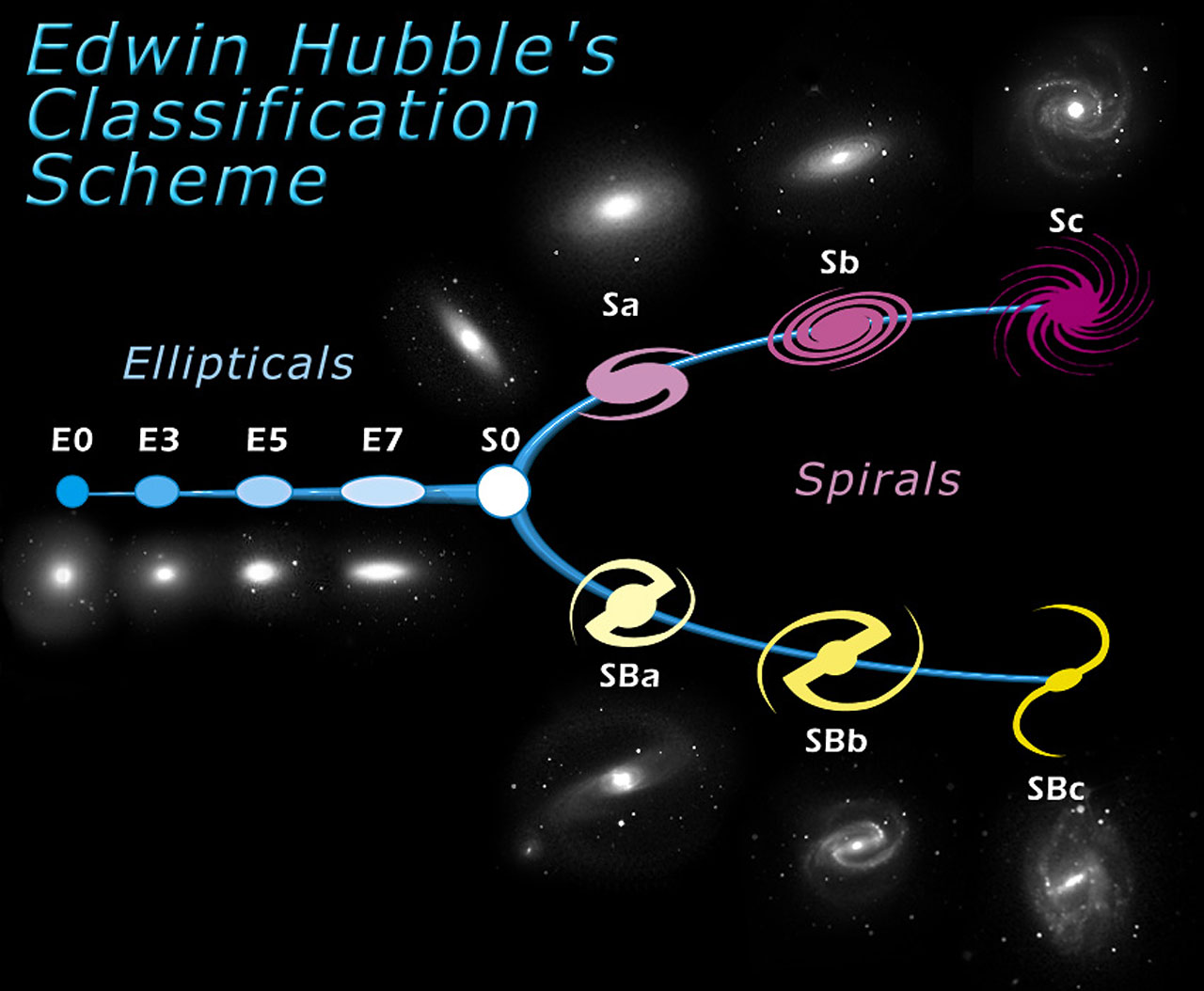
Figure 1.1: Hubble’s traditional tuning fork classification diagram for galaxies. Courtesy of the European Space Agency (ESA) http://www.spacetelescope.org/images/heic9902o/ Galaxies are defined as elliptical (E) or spiral (s) with further division of spirals into normal or barred (Sb)

The classification of galaxies turned out to be more complicated than Hubble could have envisaged. In the Hubble classification galaxies are elliptical (E) or spiral (S). Spirals also include barred galaxies where the spiral arms emerge from the tips of an elongated central layer, rather than the central bulge. It may not always be certain whether a galaxy, which appears elliptical as viewed from our solar system, is not in fact a spiral, viewed face on. Subsequently van den Bergh (1976) revised Hubble’s morphological classification of galaxies, but more recently Cappellari et al. (2011), using the ATLAS^3D astronomical survey, proposed a more physical classification based on the kinematic properties of galaxies. Their revised classification diagram is shown in Fig. 1.2.

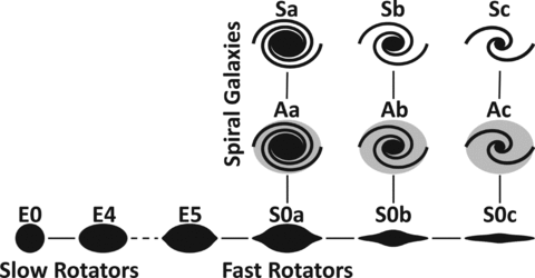
Figure 1.2: The revised galaxy classification diagram of Cappellari et al. (2011) using the ATLAS^3D astronomical survey. Galaxies are categorized as slow rotators, corresponding to elliptical shapes and fast rotators, which become increasingly flattened with smaller central bulge as a result of higher angular momentum.

Considering the kinematic properties of the galaxies improves the consistency of classification and reduces the reliance for identification on our viewing angle. It also helps us to understand the underlying cause for the variation in morphology. Disc galaxies rotate faster and, significantly, about a single axis of rotation. In some cases elliptical galaxies exhibit very weak rotation. In others the shape is the result of multiple axes of rotation, with angular momentum acting in two or three transverse directions. This action counteracts the tendency to flatten perpendicular to an axis of rotation.

Cappellari et al. (2011) found only a very small proportion of galaxies are actually elliptical (about 4% in most clusters) and the rate of rotation as well as stellar density is very important to the morphology the strength of the magnetic field. It is my long term aim to model the ISM in any class of galaxy, although the current model is constructed to simulate spiral galaxies. The most comprehensive data pertains to the Galaxy, so as a first iteration with which we can verify the relevance of the model, it is convenient to use parameters matching the Galaxy in the solar neighbourhood and compare the outcomes with what we understand of the real Galaxy.

The Galaxy is estimated to have a stellar disc of radius approximately 16 kiloparsecs (kpc) with atomic hydrogen Hi up to 40 kpc, and the Sun, is estimated to be 7 – 9 kpc from the Galactic centre. (Here capitalised Sun denotes our own star.) Most of the mass in the Galaxy is in the form of non-interacting dark matter and stars, with stars accounting for about 90% of the visible mass with gas and dust the other 10%. There is a large central bulge and although hard to identify from our position inside the Galaxy, it is likely that we live in a barred galaxy. Away from the centre most of the mass is contained within a thin disc $\pm 200$ parsecs (pc) of the mid-plane (Kulkarni and Heiles, 1987; Clemens, Sanders and Scoville, 1988; Bronfman et al., 1988; Ferrière, 2001) over a Galactocentric radius of about 4 – 12 kpc. Either side of the disc is a region referred to as the galactic halo with height of order 10 kpc. Halo gas is generally more diffuse and hotter gas in the disc.

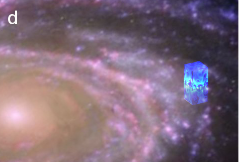
Figure 1.3: Images of spiral galaxies M81 (a), Whirlpool (b), and the barred spiral galaxy NGC 1300 (c) from %****␣intro.tex␣Line␣125␣****http://hubblesite.org/gallery/album/galaxy/ The image in panel (d) represents the typical location of the simulation region, superimposed as a blue box, orbiting the galaxy within the mid-plane of the disc. It extends above and below the mid-plane.

Figure 1.3 shows examples of disc galaxies, in panels (a – c). Panel d indicates the typical location and size of the simulation region in a galaxy, which will be described in Part II. Here the disc is rotating around the axis at about $230\,{\rm km\,s^{-1}}$ (for the Galaxy in the solar neighbourhood). As the ISM nearer to the centre of a galaxy travels a shorter orbit, differential rotation induces a shear through the ISM in the azimuthal direction, with the ISM trailing further away from the galactic centre. Rotation and shear vary between different galaxies, and also over different radii within each galaxy. These features can affect the classification of a galaxy and appear to be important to the strength and organization of the magnetic field.

1.2.2 The interstellar medium

The space between the stars is filled with a tenuous gas, the interstellar medium (ISM), which is mainly hydrogen (90.8% by number [70.4% by mass]) and helium (9.1% [28.1%]), with much smaller amounts of heavier elements also present and a very small proportion of the hydrogen in molecular form (Ferrière, 2001). The density of the ISM in the thin disc is on average below 1 atom $\,{\rm cm^{-3}}$. (In air at sea level the gas number density is about $10^{27}\,{\rm cm^{-3}}$.) The ISM contains gas with a huge range in density and temperature, and can be described as a set of phases each with distinct characteristics.

The multi-phase nature of the ISM affects all of its properties, including its evolution, star formation rate, galactic winds and fountains, and behaviour of the magnetic fields, which in turn feed back into the cosmic rays. In a widely accepted picture (Cox and Smith, 1974; McKee and Ostriker, 1977), most of the volume is occupied by the hot ($T\simeq 10^{6}\,{\rm K}$), warm ($T\simeq 10^{4}\,{\rm K}$) and cold ($T\simeq 10^{2}\,{\rm K}$) phases. The concept of the multi-phase ISM in pressure equilibrium has endured with modest refinement (Cox, 2005). Perturbed cold gas is quick to return to equilibrium due to short cooling times, while warm diffuse gas with longer cooling times has persistent transient states significantly out of thermal pressure balance (Kalberla and Kerp, 2009, and references therein). Dense molecular clouds, while containing most of the total mass of the interstellar gas, occupy a negligible fraction of the total volume and are of key importance for star formation (e.g. Kulkarni and Heiles, 1987, 1988; Spitzer, 1990; McKee, 1995). Gas that does not form one of the three main, stable phases but is in a transient state, may also be important in some processes. The main sources of energy maintaining this complex structure are supernova explosions (SNe) and stellar winds (Mac Low and Klessen, 2004, and references therein). The clustering of SNe in OB associations facilitates the escape of the hot gas into the halo thus reducing the volume filling factor of the hot gas in the disc, perhaps down to 10% at the mid-plane (Norman and Ikeuchi, 1989). The energy injected by the SNe not only produces the hot gas but also drives compressible turbulence in all phases, as well as driving outflows from the disc associated with the galactic wind or fountain, as first suggested by Bregman (1980). Thus turbulence, the multi-phase structure, and the disc-halo connection are intrinsically related features of the ISM.

Although accounting for only about 10% of the total visible mass in galaxies, the turbulent ISM is nevertheless important to their dynamics and structure. Heavy elements are forged by successive generations of stars. These are recycled into the ISM by SN feedback and transported by the ISM around the galaxy to form new stars. The ISM supports the amplification and regulation of a magnetic field, which also affects the movement of gas and subsequent location of new stars. Heating and shock waves within the ISM, primarily driven by supernovae, results in thermal and turbulent pressure alongside magnetic and cosmic ray pressure, which supports the disc against gravitational collapse.

Chapter 2 A brief review of interstellar modelling

2.1 Introduction

Work to produce a comprehensive description of the complex dynamics of the multi-phase ISM has been significantly advanced by numerical simulations in the last three decades, starting with Chiang and Prendergast (1985), followed by many others including Rosen, Bregman and Norman (1993); Rosen and Bregman (1995); Vázquez-Semadeni, Passot and Pouquet (1995); Passot, Vázquez-Semadeni and Pouquet (1995); Rosen, Bregman and Kelson (1996); Korpi, Brandenburg, Shukurov, Tuominen and Nordlund (1999); Gazol-Patiño and Passot (1999); Wada and Norman (1999); de Avillez (2000); Wada and Norman (2001); de Avillez and Berry (2001); de Avillez and Mac Low (2002); Wada, Meurer and Norman (2002); de Avillez and Breitschwerdt (2004); Balsara et al. (2004); de Avillez and Breitschwerdt (2005a, b); Slyz et al. (2005); Mac Low et al. (2005); Joung and Mac Low (2006); de Avillez and Breitschwerdt (2007); Wada and Norman (2007); Gressel et al. (2008a); Hill et al. (2012).

Numerical simulations of this type are demanding even with the best computers and numerical methods available. The self-regulation cycle of the ISM includes physical processes spanning enormous ranges of gas temperature and density, as well as requiring a broad range of spatial and temporal scales. It involves star formation in the cores of molecular clouds, assisted by gravitational and thermal instabilities at larger scales, which evolve against the global background of transonic turbulence, in turn, driven by star formation and subsequent SNe (Mac Low and Klessen, 2004). It is understandable that none of the existing numerical models cover the whole range of parameters, scales and physical processes known to be important.

Two major approaches in earlier work focus either on the dynamics of diffuse gas or on dense molecular clouds. In this chapter I will review a range of previous and current models, relating them to the physical features they include or omit. As with the general structure of the thesis, it is the extent to which physical processes are investigated that is of most interest, therefore I shall consider the physical problems and detail how various numerical approaches have been applied to these.

2.2 Star formation and condensation of molecular clouds

I shall not explicitly consider star formation. This occurs in the most dense clouds, which form from compressions in the turbulent ISM. As densities and temperatures attain critical levels in the clouds the effects of self-gravity and thermal instability may accelerate the collapse of regions within the clouds to form massive objects, which eventually ignite under high pressures to form stars.

The clouds themselves typically occupy regions spanning only a few parsecs. The final stages of star formation occurs on scales many magnitudes smaller than that, which may be regarded as infinitesimal by comparison to the dynamics of the galactic rotation and disc-halo interaction. Bonnell et al. (2006) model star formation by identifying regions of self gravitating gas of number density above $10^{5}\,{\rm cm^{-3}}$ and size$\leq 0.5\,{\rm pc}$. To track the evolution of even one star, requires very powerful computing facilities, and a time resolution well below 1 year. Currently this excludes the possibility of simultaneously modelling larger scale interstellar dynamics.

Modelling on the scale of molecular clouds, incorporating subsonic and supersonic turbulence and self-gravity is reported in Klessen, Heitsch and Mac Low (2000) and Heitsch, Mac Low and Klessen (2001) with and without magnetic field. These authors investigated the effect of various regimes of turbulence on the formation of multiple high density regions, which may then be expected to form stars. The subsequent collapse into stars was beyond the resolution of these models. Magnetic tension inhibited star formation, but this was subordinate to the effect of supersonic turbulence, which enhanced the clustering of gas within the clouds. These clusters provide the seed for star formation. In these models, supersonic turbulence was imposed by a numerical prescription. Physically the primary drivers of turbulence are SNe, and these evolve on scales significantly larger than the computational domain, so it would be difficult to include SNe and the fine structure of molecular clouds in the same model.

In addition to compression and self-gravity, thermal instability may also accelerate the formation of high density structures within the ISM. Brandenburg, Korpi and Mee (2007) investigated the effects of turbulence and thermal instability, including scales below 1 pc. Their analysis concluded that turbulent compression dominated that of thermal instability in the formation of the densest regions. The minimum cooling times were far longer than the typical turnover time of the turbulence.

Slyz et al. (2005) included star formation and a thermally unstable cooling function with a numerical domain spanning 1.28 kpc. The typical resolution was 10 or 20 pc. As previously stated, the dynamics of compression at higher resolution substantially dominate those of self-gravity and thermal instability. At this resolution, maximum density was about $10^{2}\,{\rm cm^{-3}}$ and minimum temperatures were above 300. They found a sensitivity in their results to the inclusion or exclusion of self-gravity, which Heitsch, Mac Low and Klessen (2001), with higher resolution, found to be subordinate to the effects of turbulence on the density profile. I would argue that this indicates that including self-gravity at such large scales may therefore produce artificial numerical rather than physical effects. The gravitational effect of the ISM on scales greater than 1 pc are negligible, compared to stellar gravity and other dynamical effects.

In summary, modelling star formation and molecular clouds in the ISM necessitates a resolution significantly less than 1 pc. Self-gravity within the ISM is significant only for dense structures inside molecular clouds. Such gravitation is proportional to $l^{-2}$, where $l$ denotes the distance from some mass sink, so is a highly localised phenomenon. Star formation in large scale modelling can therefore at best be parametrized by the removal of mass from the ISM based on the distribution of dense mass structures and self-gravity neglected.

2.3 Discs and spiral arms

To model a whole spiral galaxy requires a domain radius of order $10\,{\rm kpc}$ and potentially double that in height to include the halo. Often to avoid excessive computation, when modelling scales spanning the whole disc some authors either adopt a 2D horizontal approach (Slyz, Kranz and Rix, 2003), or adopt a very low vertical extent in 3D (Dobbs and Price, 2008; Hanasz, Wóltański and Kowalik, 2009; Kulesza-Żydzik et al., 2009; Dobbs and Pringle, 2010). Given the mass, energy and turbulence are predominantly located within a few hundred parsecs of the mid-plane, some progress can be made with this approach.

A number of important physical features of the ISM must be neglected at this resolution. An important factor in the self-regulation of the ISM is the galactic fountain, in which over-pressured hot gas in the disc is convected into the halo, where it cools and rains back to the disc. How this affects star-formation and SNe rates is poorly understood.

The multi-phase ISM cannot currently be resolved at these scales. The cold diffuse gas exists in clumpy patches of at most a few parsecs. Even the hot bubbles of gas, generated at the disc by SNe and clusters of SNe are typically less than a few hundred parsecs across. The resolution of these global models is of order 100 pc, which is insufficient to include the separation of scales of about $10^{3}$ between the hot and the warm gas. Generally these models apply an isothermal ISM. Dobbs and Price (2008) include a multiphase medium, by defining cold and warm particles, with fixed temperature and density, but must exclude any interaction between the phases.

The random turbulence driven by SNe must also be neglected or weakly parametrized. Dobbs and Price (2008) exclude SNe with the effect of significantly reducing the disc height between the spiral arms. Hanasz, Wóltański and Kowalik (2009) neglect the thermal and kinetic energy and inject energy only through current rings of radius 50 pc and 1% of the total SN energy. Slyz, Kranz and Rix (2003) use forced supersonic random turbulence to generate density perturbations.

These models can reproduce structures similar to spiral arms and, where a magnetic field is included, an ordered field on the scale of the spiral arms. These can be related to different rates of rotation and for various density profiles. Even in 3D however these only describe the flat 2D structure of the disc and spiral arms. Both the velocity and the magnetic fields are vectors and subject to non-trivial transverse effects. The effect of asymmetry on these vectors in the vertical direction cannot be well represented with this geometry.

Features such as the vertical density distribution of the ISM, the thermal properties and turbulent velocities cannot be understood from these models. They must be introduced as model parameters, derived from observational measurements or smaller scale simulations. On the other hand structures such as spiral arms are too large to generate in more localised simulations. The global simulations may help to identify suitable parameters for introducing spiral arms into local models, such as the scale of the density fluctuations, orientation of the arms, typical width of the arms, how the strength or orientation of the magnetic field varies between the arm and interarm regions.

2.4 The multi-SNe environment

This thesis concerns modelling the ISM in a domain larger than the size of molecular clouds (Sect 2.2) and much smaller than a galaxy, or even just the disc (Sect 2.3). Models on this scale were introduced by Rosen, Bregman and Norman (1993), in 2D with much lower resolution, and without SNe. Nonetheless these already were able to identify features of the galactic fountain and the multiphase structure of the ISM. Individual SNe were investigated numerically by Cowie, McKee and Ostriker (1981). Extensive high resolution simulations led to the refinement of the classic Sedov-Taylor solution (Sedov, 1959; Taylor, 1950) and subsequent snowplough describing the evolution of an expanding blast wave (Ostriker and McKee, 1988; Cioffi, McKee and Bertschinger, 1998). The modelling of multiple SNe in the form of superbubbles within a stratified ISM was advanced by Tomisaka (1998). The first 3D simulations of SNe driven turbulence in the ISM were by Korpi, Brandenburg, Shukurov, Tuominen and Nordlund (1999) and, independently, de Avillez (2000). In this section I consider the key physical and numerical elements of these and subsequent similar models, and the extent to which their inclusion or omission improves or hinders the results.

2.4.1 The stratified interstellar medium

From the images in Fig.1.3 and the profiles illustrated in Fig. 1.2 it can be seen that the matter in spiral galaxies is substantially flattened into a disc. This morphology strongly depends on the rate and form of rotation of the galaxy. Towards the centre of these galaxies is a bulge, where the density structure and dynamics differ substantially from those in the disc. In elliptical galaxies the structure may involve asymmetries that are complicated to model. I shall defer consideration of the central region and elliptical galaxies to elsewhere and confine this thesis to the investigation of the disc region of fast rotating galaxies.

Along the extended plane of the disc in fast rotators the dense region of gas may reasonably be approximated as unstratified to within about a few hundred parsecs of the mid-plane depending on the galaxy. The thickness of the disc away from the central bulge can, in many cases, to first approximation be regarded as constant, although it does usually increase exponentially away from the galactic centre. Thus, towards the outer galaxy, even over relatively short distances the flat disc approximation breaks down. Providing the model domain remains sufficiently within the thickness of the disc, some progress can be made by ignoring stratification, (eg Balsara et al., 2004; Balsara and Kim, 2005).

Important to the dynamics of the interstellar medium is its separation into characteristic phases in apparent pressure equilibrium. Is this separation a real physical effect, or just a statistical noise? What are the thermodynamical properties of the gas, what are the filling factors, typical motions and, if the phases do in fact differ qualitatively, how do they interact? The answers to these questions are critically different when considering the ISM to be stratified or not. Balsara et al. (2004) investigated the effect of increasing rates of supernovae on the composition of the ISM. With initial density set to match the mid-plane of the Galaxy, increasing the rate of energy injection resulted in increased proportions of cold dense and hot diffuse gas and correspondingly less warm gas. The typical radius of SN remnant shells in such a dense medium remained below 50 pc before being absorbed into the surrounding turbulence. The result of increased SNe is higher pressures and eventually overheating of the ISM.

However when a stratified ISM is included, the increased pressure from SNe near the mid-plane is released away from the disc, by a combination of diffuse convection and blow outs of hot high pressure bubbles. Korpi, Brandenburg, Shukurov and Tuominen (1999); de Avillez (2000); de Avillez and Berry (2001) included stratification. They found superbubbles, which combine multiple SNe merging or exploding inside existing remnants in the disc and then breaking out into the more diffuse layers, where they transport the hot gas away. They also had individual SNe exploding at distances $\,\hbox to0.0pt{\raise 2.15277pt\hbox{$>$}\hss}{\lower 4.30554pt\hbox{$\sim$}}\,500\,{\rm pc}$ from the mid-plane, where the ambient ISM is very diffuse and the remnants of these SNe extend to a radius of a few hundred parsecs. This also has an effect on the typical pressures, turbulent velocities and mixing scales. Instead of the cold gas and hot gas becoming more abundant at the mid-plane, the hot gas is transported away and the thickness of the disc expands reducing the mean density and mean temperature at the mid-plane.

Due to the gravitational potential, dominated by stellar mass near the mid-plane, there is a vertical density and pressure gradient. This will vary depending on the galaxy, but in most simulations of this nature it is useful to adopt the local parameters, since data relating to the solar neighbourhood is generally better understood, and therefore is convenient for benchmarking the results of numerical simulations.

There is a natural tendency for cold dense gas to be attracted to the mid-plane and hot diffuse gas to rise and cool. Estimates from observations in the solar vicinity place the Gaussian scale height of the cold molecular gas at about $80\,{\rm pc}$ and the neutral atomic hydrogen about $180\,{\rm pc}$ (Ferrière, 2001). The warm gas is estimated to have an exponential scale height of $390-1000\,{\rm pc}$. Observationally hot gas is more difficult to isolate and estimates vary for the exponential scale height; ranging from as low as 1 kpc to over 5 kpc. Hence to reasonably produce the interaction between the cold and warm gas, we at least need to extend $\pm 1\,{\rm kpc}$ vertically. de Avillez (2000) with a vertical extent of $\pm 4\,{\rm kpc}$ found the ISM above about 2.5 kpc to be 100% comprised of hot gas, and this vertical extent was not high enough to observe the cooling and recycling of the hot gas back to the disc. Subsequent models (including de Avillez and Mac Low, 2001; de Avillez and Berry, 2001; de Avillez and Mac Low, 2002; Joung and Mac Low, 2006; Joung, Mac Low and Bryan, 2009; Hill et al., 2012) use an extended range in $z$ of $\pm 10\,{\rm kpc}$ and find the volume above about $\pm 2.5\,{\rm kpc}$ almost exclusively occupied by the hot gas for column densities and SNe rates comparable to the solar vicinity. Many of these models exclude the magnetic field and all exclude cosmic rays so the models have somewhat thinner discs than expected from observations. With the inclusion of magnetic and cosmic ray pressure, we expect the disc to be somewhat thicker and the scale height of the hot gas to increase.

The build up of thermal and turbulent pressure by SNe near the mid-plane generates strong vertical flows of the hot gas towards the halo. With vertical domain $|z|=10\,{\rm kpc}$ de Avillez and Breitschwerdt (2004) are able to attain an equilibrium with hot gas cooling sufficiently to be recycled back to the mid-plane, replenishing the star forming regions and subsequently SNe. Such recycling may be expected to occur in the form of a galactic fountain. However Korpi, Brandenburg, Shukurov and Tuominen (1999); Korpi, Brandenburg, Shukurov, Tuominen and Nordlund (1999) found the correlation scale in the warm gas of the velocity field remained quite consistently about 30 pc independent of $z$ location, but in the hot gas it increased from about 20 pc at the mid-plane to over 150 pc at $|z|\simeq 300\,{\rm pc}$ and increasing with height. Other authors report correlation scales similar near the mid-plane, but the vertical dependence of correlation lengths requires further investigation. If there is an increase in the correlation length of the velocity field with height, as $|z|\rightarrow 1\,{\rm kpc}$ the scale of the turbulent structures of the ISM can become comparable to the typical size of the numerical domain. Consequently in extending the $z$-range to include the vertical dimension of the hot gas, its horizontal extent may exceed the width of too narrow a numerical box. With a vertical extent of only $\pm 1\,{\rm kpc}$, or with Gressel et al. (2008a) $\pm 2\,{\rm kpc}$, there is a net outflow of gas. Without a mechanism for recycling the hot gas, net losses eventually exhaust the disc and the model parameters cease to be useful. Korpi, Brandenburg, Shukurov, Tuominen and Nordlund (1999) found this restriction limited the useful time frame to a few hundred Myr. It is difficult to combine in one model the detailed dynamics of the SNe driven turbulence about the mid-plane with a realistic global mechanism for the recycling of the hot gas.

There has also been some discussion on the effect of magnetic tension inhibiting these outflows. Using 3D simulations of a stratified but non-turbulent ISM with a purely horizontal magnetic field Tomisaka (1998) placed an upper bound on this confinement. When the ISM is turbulent the magnetic field becomes disordered, the ISM contains pockets of diffuse gas, and the opportunity for hot gas blow outs increases substantially (see e.g. Korpi, Brandenburg, Shukurov and Tuominen, 1999; de Avillez and Breitschwerdt, 2004, 2005b).

2.4.2 Compressible flows and shock handling

The ISM is highly compressible, with much of the gas moving at supersonic velocities. The most powerful shocks are driven by SNe. Accurate modelling of a single SNe in 3D requires high resolution and short time steps (Ostriker and McKee, 1988). On the scales of interest here, hundreds or thousands of SNe are required and this constrains the time and resolution available to model the SNe. Approximations need to be made, which retain the essential characteristics of the blast waves and structure of the remnants at the minimum physical scales resolved by the model.

Shock handling is optimised (by e.g. de Avillez, 2000; Balsara et al., 2004; Mac Low and Klessen, 2004; Joung and Mac Low, 2006; Gressel et al., 2008a) through adaptive mesh refinement (AMR), where increased resolution is applied locally for regions containing the strongest contrasts in density, temperature or flow. With increased spatial resolution the time step must also be much smaller, so there are considerable computational overheads to the procedure. Many of the codes utilising AMR do not currently include modelling of differential rotation, although Gressel et al. (2008a) does apply shear using the Nirvana code. An alternative approach is to apply enhanced viscosities where there are strong convergent flows (by e.g. Korpi, Brandenburg, Shukurov, Tuominen and Nordlund, 1999). This broadens the shock profiles and removes discontinuities, so care needs to be taken that essential physical properties are not compromised.

2.4.3 Distribution and modelling of SNe

There are a number of different types of supernovae, with different properties and origin. Type Ia SNe arise from white dwarfs, which are older stars that have used up most of their hydrogen and comprise mainly of heavier elements oxygen and carbon. If, through accretion or other mechanisms, their mass exceeds the Chandrasekhar limit (Chandrasekhar, 1931) of approximately $1.38M\odot$ they become unstable and explode. Type Ia are observed in all categories of galaxy and can have locations isolated from other types of SNe.

Type II SNe are produced by massive, typically more than $10M\odot$, relatively young hot stars, which rapidly exhaust their fuel and collapse under their own gravity before exploding. Type Ib and Ic are characterized by the absence of hydrogen lines in their spectrum and, for Ic, also their helium, which has been stripped by either stellar winds or accretion, before the more dense residual elements collapse to form SNe. Otherwise Type II, Ib and Ic SNe are very similar, located only in fast rotating galaxies and populating mainly the star forming dense gas clouds near the mid-plane of the disc. For the remainder of this thesis I shall collectively denote these as Type CC (core collapsing) and Type I shall refer only to Type Ia. Type CC SNe are more strongly correlated in space and time than Type I, because they form in clusters, evolve over a few million years and explode in rapid succession.

In many disc galaxies, including the Milky Way, Type CC SNe are much more prolific than Type I. Both types effectively inject $10^{51}\,{\rm erg}$ into the ISM (equivalent to $10^{40}$ modern thermo-nuclear warheads exploded simultaneously). Type CC also contribute $4-20M\odot$ as ejecta at supersonic speeds of a few thousand $\,{\rm km\,s^{-1}}$. Mainly located in the most dense region of the disc, Type CC SNe energy can be more rapidly absorbed and explosion sites reach a radius of typically 50 pc before becoming subsonic, while some Type I explode in more diffuse gas away from the mid-plane and can expand to a radius of a few hundred parsecs. Because Type CC are correlated in location and time, many explode into or close to existing remnants and form superbubbles of hot gas, which help to break up the dense gas shells of SN remants and increase the turbulence. Heating outside the mid-plane by Type I SNe helps to disrupt the thick disc and increase the circulation of gas from within.

A common prescription for location of SNe in numerical models, is to locate them randomly, but uniformly in the horizontal plane and to apply a Gaussian or exponential random probability distribution in the vertical direction, with its peak at the mid-plane $z=0$. Having determined the location, an explosion is then modelled by injecting a roughly spherical region containing mass, energy and/or a divergent velocity profile. The sphere needs to be large enough, that for the given resolution, the resulting thermal and velocity gradients are numerically resolved. This means that for typical resolution of a few pc the radius of the injection site will be several parsecs and indicative of the late Sedov-Taylor or early snowplough phase (See Section 3.2 and Appendix A.1) some thousands of years after the explosion. Subsequently gas is expelled by thermal pressure or kinetic energy from the interior to form an expanding supersonic shell, which drives turbulent motions and heats up the ambient ISM. Problems have been encountered with modelling the subsequent evolution of these remnants. Cooling can dissipate the energy before the remnant shell is formed. Using kinetic rather than thermal energy to drive the SNe evolution is hampered by the lack of resolution.

As well as being physically consistent, clustering of SNe mitigate against energy losses by ensuring they explode in the more diffuse, hot gas where they are subject to lower radiative losses. To achieve clustering for the Type CC SNe Korpi, Brandenburg, Shukurov and Tuominen (1999) selected sites with a random exponential distribution in $z$, excluded sites in the horizontal plane with density below average for the layer and then applied uniform random selection. de Avillez (2000) apply a more rigorous prescription to locate 60% of Type CC in superbubbles, in line with observational estimates (Cowie, Songaila and York, 1979). In addition to a simplified clustering scheme Joung and Mac Low (2006) and Joung, Mac Low and Bryan (2009) also adjust the radii of their SNe injection sites to enclose $60M\odot$ of ambient gas. This appears to optimise the efficiency of the SNe modelling; avoiding high energy losses at $T>10^{8}\,{\rm K}$ with a smaller injection site or avoiding too large an injection site, which dissipates the energy before the snowplough phase can be properly reproduced.

The critical features of the SNe modelling must ensure that the SNe are sufficiently energetic and robust to stir and heat the ambient ISM. It is unlikely that the individual remnants can be accurate in every detail, given the constraints on time and space resolution, but the growth of the remnants should be physically consistent, producing remnants and bubbles of multiple remnants at the appropriate scale. In particular we can expect about 10% of the energy to be output into the ISM in the form of kinetic energy when the remnant merges with the ambient ISM. Spitzer (1978) estimates this to be 3% and Dyson and Williams (1997) to be 30%.

2.4.4 Solid body and differential rotation

To understand the density and temperature composition of the ISM the inclusion of the rotation of the galaxy is not essential. Even an appreciation of the characteristic velocities and Mach numbers associated with the regions of varying density or temperature can be obtained without rotation. Balsara et al. (2004); Balsara and Kim (2005); Mac Low et al. (2005) and de Avillez and Breitschwerdt (2005a) investigate the magnetic field in the ISM without rotation or shear, the latter in the vertically extended stratified ISM, otherwise in an unstratified $(200\,{\rm pc})^{3}$ section. The latter two models impose a uniform $B$ of between $2-5\,\umu{\rm G}$. The turbulence breaks up the ordered field (mean denoted ${{\mbox{\boldmath$B$}}}_{0}$) and with modest amplification of the total magnitude $B$, although the simulations last only a few hundred Myr. Over a longer period, it would be expected that ${{\mbox{\boldmath$B$}}}_{0}$ would continue to dissipate in the absence of any restoring mechanism (rotation). They analyze the distribution with respect to density and temperature of the fluctuations, $b$, and mean parts of the field, and their comparative strengths.

Balsara et al. (2004) and Balsara and Kim (2005) investigate the fluctuation dynamo, introducing a seed field of order $10^{-3}\,\umu{\rm G}$ and increasing it to $10^{-1}\,\umu{\rm G}$ over 40 Myr. This is insufficiently long to saturate and there is no mean field, but they do examine the turbulent structure of $b$ and the dynamo process.

However galactic differential rotation is a defining feature of the global characteristics of disc galaxies and is felt locally by the Coriolis effect and shearing in the azimuthal direction. There is observational evidence that the magnetic field in disc galaxies, which is heavily randomised by turbulence, is also strongly organized along the direction of the spiral arms (e.g. Patrikeev et al., 2006; Tabatabaei et al., 2008; Fletcher et al., 2011). Differential rotation is responsible for the spiral structure, so must be included to understand the source of the mean field in the galaxy.

There is also considerable controversy over the nature and even the existence of the the galactic dynamo. A fluctuation dynamo can be generated by turbulence alone, but it is not clear that it can be sustained indefinitely. The mean field dynamo cannot be generated without anisotropic turbulence and large scale systematic flows.

Gressel et al. (2008a, b) include differential rotation and by introducing a small seed field, are able to derive a mean field dynamo for a stratified ISM. The dynamo is only sustained in their model for rotation $4\Omega_{0}$, where $\Omega_{0}\approx 230\,{\rm km\,s^{-1}}$ is the angular velocity of the Galaxy in the solar vicinity. Otherwise they apply parameters the same as or similar to the local Galaxy. Gressel (2008) also considered solid body rotation and found no dynamo, but concluded that shear, without rotation, cannot support the galactic dynamo. Without rotation diamagnetic pumping is too weak to balance the galactic wind. The resolution of the model at $(8\,{\rm pc})^{3}$ limits the magnetic Reynolds numbers available, which may explain the failure to find a dynamo with rotation of $\Omega_{0}$. For a comprehensive understanding of the galactic magnetic field differential rotation should not be neglected.

2.4.5 Radiative cooling and diffuse heating

The multi-phase structure of the ISM would appear to be the result of a combination of the complex effects of supersonic turbulent compression, randomized heating by SNe and the differential cooling rates of the ISM in its various states. Although excluding SNe, and having a low resolution, Rosen, Bregman and Norman (1993) generated a multi-phase ISM with just diffuse stellar heating from the mid-plane and non-uniform radiative cooling.

Radiative cooling depends on the density and temperature of the gas and different absorption properties of various chemicals within the gas on the molecular level. For models such as the ones discussed here detailed analysis of these effects and estimates of the relative abundances of these elements in different regions of the ISM (see e.g. Wolfire et al., 1995) need to be adapted to fit a monatomic gas approximation. Stellar heating varies locally, on scales far below the resolution of these models, due to variations in interstellar cloud density and composition as well ambient ISM temperature sensitivities.

Subtle variations in the application of these cooling and heating approximations may have very unpredictable effects, due to the complex interactions of the density and temperature perturbations and shock waves. In particular thermal instability is understood to be significant in accelerating the gravitational collapse of dense clouds, by cooling the cold dense gas more quickly than the ambient diffuse warm gas.

Different models have used radiative cooling functions which are qualitatively as well as quantitatively distinct, making direct comparison uncertain. Vázquez-Semadeni, Gazol and Scalo (2000) compared their thermally unstable model to a different model by Scalo et al. (1998) who used a thermally stable cooling function. They concluded that thermal instability on $1\,{\rm pc}$ scales is insufficient to account for the phase separation of the ISM, but in the presence of other instabilities increases the tendency towards thermally stable temperatures. Similarly, de Avillez and Breitschwerdt (2004) and Joung and Mac Low (2006) compared results obtained with different cooling functions, but comparing models with different algorithms for the SN distribution and control of the explosions. In the absence of SNe driven turbulence the ISM does separate into two phases with reasonable pressure parity and in the presence of background turbulence this separation persists (Sánchez-Salcedo, Vázquez-Semadeni and Gazol, 2002; Brandenburg, Korpi and Mee, 2007). Although the pressure distribution broadens, the bulk of both warm and cold gases broadly retain pressure parity.

An additional complexity is advocated by de Avillez and Breitschwerdt (2010). Generally it is assumed that ionization through heating and recombination of atoms by cooling are in equilibrium. However recombination time scales lag considerably, so that cooling is not just dependent on temperature and density. Cooler gas which had been previously heated to $T>10^{6}\,{\rm K}$ will remain more ionized than gas of equivalent density and temperature which has not been previously heated. de Avillez and Breitschwerdt (2010) show that this significantly affects the radiation spectra of the gas, therefore they use a cooling function which varies locally, depending on the thermal history of the gas.

The choice of cooling and heating functions has a quantitative effect on the results of ISM models and there is evidence that the inclusion or exclusion of thermal instability in various temperature ranges has a qualitative impact on the structure of the ISM. However uncertainty remains over whether the adopted cooling functions are indeed faithfully reproducing the physical effects. There is also uncertainty over how critical the differences between various parameterizations are to the results, once SNe, magnetic fields and other processes are considered. It is certain, however, that differential radiative cooling is an essential feature of the ISM.

2.4.6 Magnetism

Estimates of the strength of magnetic fields indicate that the magnetic energy density has the same order of magnitude as the kinetic and thermal energy densities of the ISM. Including magnetic pressure substantially increases the thickness of the galactic disc compared to the purely hydrodynamic regime. Magnetic tension and the Lorentz force will affect the velocities and density perturbations in the ISM. Ohmic heating and electrical conductivity will affect the thermal composition of the ISM. Hydrodynamical models provide an excellent benchmark, but to accurately model the ISM and be able to make direct comparisons with observations the magnetic field should be included.

Comparisons between MHD and HD models have been made (Korpi, Brandenburg, Shukurov and Tuominen, 1999; Balsara et al., 2004; Balsara and Kim, 2005; Mac Low et al., 2005; de Avillez and Breitschwerdt, 2005a). These either impose a relatively strong initial mean field or contain only a random field, and are evolved over a comparatively short time frame. So the composition of the field cannot reliably be considered authentic. Ideally it would be useful to understand the dynamo mechanism; are there minimum and maximum rates of rotation conducive to magnetic fields? How does the SNe rate or distribution affect the magnetic field? What is the structure of the mean field, how do the mean and fluctuating parts of the field compare and how is the magnetic field related to the multi-phase composition of the ISM? To ensure the field is the product of the ISM dynamics the mean field needs to be generated consistently with the key ingredients of differential rotation and turbulence, from a very small seed field. The time over which the model evolves must be sufficiently long that no trace of the seed field properties persist.

2.4.7 Cosmic Rays

Cosmic rays are high energy charged particles, travelling at relativistic speeds. Their trajectories are strongly aligned to the magnetic field lines (Kulsrud, 1978). It is speculated that, amongst other potential sources, they are generated and accelerated in shock fronts around supernovae. They also occur in solar mass ejections, some of which are caught in the Earth’s magnetosphere. The polar aurora result from these travelling along the field lines and heating the upper atmosphere as they collide.

Cosmic rays are of interest in themselves, but also are estimated to make a similar contribution to the energy density and pressures in the ISM as each of the magnetic field, the kinetic and the thermal energies (Parker, 1969). As such their inclusion can be expected to significantly affect the global properties of the ISM.

Although a substantial component of the ISM is not charged the highly energized cosmic rays strongly affect the bulk motion of the gas. The interaction between cosmic rays and the ISM is highly non-linear, but can be considered in simplified form by a diffusion-advection equation,

$$\frac{\partial e_{\rm cr}}{\partial t}+\nabla(e_{\rm cr}{{\mbox{\boldmath$u$}}}) =-p_{\rm cr}\nabla{{\mbox{\boldmath$u$}}}+\nabla(\hat{K}\nabla e_{\rm cr})+Q_{\rm cr}\,,$$ (2.1)

$$p_{\rm cr} =(\gamma_{\rm cr}-1)e_{\rm cr}\,,$$ (2.2)

where $e_{\rm cr}$ and $p_{\rm cr}$ are the cosmic ray energy and pressure respectively, and $\hat{K}$ the cosmic ray diffusion tensor, $\gamma_{\rm cr}$ the cosmic ray ratio of specific heats, and $Q_{\rm cr}$ a cosmic ray source term such as SNe. $u$ is the ISM gas velocity.

Hanasz et al. (2004, 2005, 2006, 2011) use cosmic rays in a magnetized isothermal simulation to perturb the magnetic field and drive the dynamo in their global disc galaxy simulations. None of the thermodynamic, stratified models of the ISM have yet included cosmic rays.

2.4.8 Diffusivities

The dimensionless parameters characteristic of the ISM, such as the kinetic and magnetic Reynolds numbers (reflecting the relative importance of gas viscosity and electrical resistivity) and the Prandtl number (quantifying thermal conductivity) are too large to be obtainable with current computers. Lequeux (2005) estimates the Reynolds number ${\rm Re}\simeq 10^{7}$ for the cold neutral medium, with viscosity $\nu\simeq 3\times 10^{17}\,{\rm cm}^{2}\,{\rm s}^{-1}$. Uncertainty applies to these estimates in the various phases and also to thermal and magnetic diffusivities, but physical ${\rm Re}$ and $\mathrm{Rm}$ (magnetic Reynolds number) are far larger and diffusivities far smaller than can be resolved numerically. Given the very low physical diffusive co-efficients in the ISM some models approximate them as zero. Applying ideal MHD where electrical resistivity is ignored (e.g. de Avillez, 2000; Mac Low et al., 2005; Joung and Mac Low, 2006; Li, Mac Low and Klessen, 2005, and their subsequent models) the magnetic field is modelled as frozen in to the fluid. Although magnetic diffusion is not explicitly included in their equations, it exists through numerical diffusion which is determined by the grid scale. In models with adaptive mesh refinement, the diffusion varies locally with the variations in resolution.

In fact, within the turbulent environment of the ISM, although the diffusivity is very low, shocks and compressions can create conditions, in which the time scales of the diffusion are comparable with other time scales such as the diffusion of heat, charge and momentum. Korpi, Brandenburg, Shukurov, Tuominen and Nordlund (1999) and Gressel et al. (2008a) include bulk diffusivity in their equations, which are some orders of magnitude larger than those typical of the ISM. These are constrained by the minimum that can be resolved with the numerical resolution available, but ensure the level of diffusion is consistent throughout.

Although, the maximum effective Reynolds numbers are much lower than estimates for the real ISM, there is considerable consistency in structures derived by models on the meso-scales, e.g., thickness of the disc, size of remnant structures and super bubbles, typical velocities, densities and temperatures. Uncertainties are greater in describing the fine structures; remnant shells, condensing clouds, and dispersions of velocity, density and temperature.

2.4.9 The galactic fountain

It is reasonable to conclude from what we understand from observations and the work of de Avillez and Mac Low (2002) and their subsequent models, that the modelling of the galactic fountain requires a scale height of order $\pm 10\,{\rm kpc}$. They found $z=\pm 5\,{\rm kpc}$ was insufficient to establish a duty cycle with hot gas condensing and recycling back to the disc. Gressel et al. (2008a) model the ISM to $z=\pm 2\,{\rm kpc}$ and throughout their model there is a net outflow across the outer horizontal surfaces.

Less clear is how large a horizontal span is required. Korpi, Brandenburg, Shukurov, Tuominen and Nordlund (1999) found the correlation length of the velocity of the hot gas increased from about 20 pc at $z=0$ to about 150 pc at $|z|=300\,{\rm pc}$ and the scale of the box at $|z|=850\,{\rm pc}$. This indicates that as height increases above 1 kpc the size of the physical structures of the hot gas may well exceed the model. As such reliable modelling of the galactic fountain may well require a substantially larger computational domain in all directions. de Avillez and Mac Low (2002) model large $|z|$ with much lower resolution than the mid-plane, to manage the computational demands. It may be that the scale of the task may necessitate sacrificing resolution throughout to expand the range of the models to investigate the galactic fountain.

2.4.10 Spiral arms

Only models on the larger scales previously described (Slyz, Kranz and Rix, 2003; Dobbs and Price, 2008; Hanasz et al., 2004, and subsequent models) have reproduced features similar to the spiral arms in rotating galaxies. It is unlikely that the dynamics of the spiral arms can be understood from models in the scale of 1–2 kpc in the horizontal, because they are structures typical of the full size of the galaxy. Rather than an outcome of such models, they could perhaps be included as an input in the form of a density wave through the box at appropriate intervals, with other associated effects, such as fluctuations in SNe rates.

2.5 Summary

Many models have been used, some to describe different astrohpysical features or alternative approaches to the same environment. Direct comparison of results is consequently difficult. All models must omit ingredients and approximate or parameterize some of the challenging dynamics. Computational power restricts resolution, domain size and physical components, so each model must be adapted to match the requirements of the particular astrophysics under investigation; e.g. star formation permits only a small domain, enables high resolution, requires thermal instability; spiral arms impose the requirement of a global domain, restrict resolution or turbulence. A comprehensive understanding requires a heirarchy of models, spanning an overlapping range of scales, encompassing the all the critical physical features.

Part II Modelling the interstellar medium

Chapter 3 Basic equations and their numerical implementation

3.1 Basic equations

I solve numerically a system of equations using the Pencil Code , which is designed for fully nonlinear, compressible magnetohydrodynamic (MHD) simulations. I do not currently include cosmic rays, which will be considered elsewhere subsequently.

The basic equations include the mass conservation equation, the Navier–Stokes equation (written here in the rotating frame), the heat equation and the induction equation:

$$\frac{D\rho}{Dt}\, =\,-\nabla\cdot(\rho{{\mbox{\boldmath$u$}}})\,+\dot{\rho}_{\rm SN},$$ (3.1)

$$\frac{D{{\mbox{\boldmath$u$}}}}{Dt}\, =\,-\rho^{-1}\nabla{\sigma}_{\rm SN,kin}\,-c{{}_{\mathrm{s}}}^{2}\nabla\left({s}/{\,{c_{\rm p}}}+\ln\rho\right)\,-\nabla\Phi\,-Su_{x}\bm{\hat{y}}\,-2{{\mbox{\boldmath$\Omega$}}}\times{{\mbox{\boldmath$u$}}}$$

$$\,+\,\rho^{-1}{{\mbox{\boldmath$j$}}}\times{{\mbox{\boldmath$B$}}}\,+\nu\left(\nabla^{2}{{\mbox{\boldmath$u$}}}+{\textstyle{\frac{1}{3}}}\nabla\nabla\cdot{{\mbox{\boldmath$u$}}}+2{\textbf{{W}}}\cdot\nabla\ln\rho\right)\,+\zeta_{\nu}\left(\nabla\nabla\cdot{{\mbox{\boldmath$u$}}}\right),$$ (3.2)

$$\rho T\frac{Ds}{Dt}\, =\,\dot{\sigma}_{\rm SN,th}\,+\rho\Gamma\,-\rho^{2}\Lambda\,+\nabla\cdot\left(\,{c_{\rm p}}\rho\chi\nabla T\right)\,+\eta\mu_{0}{{\mbox{\boldmath$j$}}}^{2}$$

$$\,+\,2\rho\nu\left|{\textbf{{W}}}\right|^{2}+\zeta_{\chi}\left(\rho T\nabla^{2}s+\nabla\ln\rho T\cdot\nabla s\right)+\rho T\nabla\zeta_{\chi}\cdot\nabla s,$$ (3.3)

$${\color[rgb]{0,0,0}{\frac{\partial{{\mbox{\boldmath$A$}}}}{\partial t}}}\, =\,{\color[rgb]{0,0,0}{{{\mbox{\boldmath$u$}}}\times{{\mbox{\boldmath$B$}}}\,-SA_{y}{{\mbox{\boldmath$\hat{x}$}}}\,-Sx\frac{\partial{{\mbox{\boldmath$A$}}}}{\partial y}}}$$

$$\,+\,(\eta+\zeta_{\eta})\nabla^{2}{{\mbox{\boldmath$A$}}}\,+\nabla\cdot{{\mbox{\boldmath$A$}}}({\color[rgb]{0,0,0}{\nabla\eta+}}\nabla\zeta_{\eta}),$$ (3.4)

where $\rho$, $T$ and $s$ are the gas density, temperature and specific entropy, respectively, $u$ is the deviation of the gas velocity from the background rotation profile (here called the velocity perturbation), and $B$ and $A$ are the magnetic field and magnetic potential, respectively, such that ${{\mbox{\boldmath$B$}}}=\nabla\times{{\mbox{\boldmath$A$}}}$. Also $j$ is the current density, $c{{}_{\mathrm{s}}}$ is the adiabatic speed of sound, $\,{c_{\rm p}}$ is the heat capacity at constant pressure, $S$ is the velocity shear rate associated with the Galactic differential rotation at the angular velocity $\Omega$ (see below), assumed to be aligned with the $z$-axis. The Navier–Stokes equation includes the viscous term with the viscosity $\nu$ and the rate of strain tensor W whose components are given by

$$2W_{ij}=\frac{\upartial u_{i}}{\upartial x_{j}}+\frac{\upartial u_{j}}{\upartial x_{i}}-\frac{2}{3}\delta_{ij}\nabla\cdot{{\mbox{\boldmath$u$}}},$$

as well as the shock-capturing viscosity $\zeta_{\nu}$ and the Lorentz force, $\rho^{-1}{{\mbox{\boldmath$j$}}}\times{{\mbox{\boldmath$B$}}}$. The implementation of shock-capturing is discussed in Section 3.4

The system is driven by SN energy injection per unit volume, at rates $\dot{\sigma}_{\rm SN,kin}$ in the form of kinetic energy in Eq. (3.1) and thermal energy ($\dot{\sigma}_{\rm SN,th}$) in Eq. (3.1). Energy injection is confined to the interiors of SN remnants, and the total energy injected per supernova is denoted $E_{\rm SN}$. The mass of the SN ejecta is included in Eq. (3.1) via the source $\dot{\rho}_{\rm SN}$. The forms of these terms are specified and further details are given in Section 3.2.

The heat equation also contains a thermal energy source due to photoelectric heating $\rho\Gamma$, energy loss due to optically thin radiative cooling $\rho^{2}\Lambda$, heat conduction with the thermal diffusivity $\chi$, viscous heating (with $|{\textbf{{W}}}|$ the determinant of W), Ohmic heating $\eta\mu_{0}{{\mbox{\boldmath$j$}}}^{2}$, and the shock-capturing thermal diffusivity $\zeta_{\chi}$. $K=\,{c_{\rm p}}\rho\chi$ is the thermal conductivity and $\mu_{0}$ is vacuum permeability.

The induction equation includes magnetic diffusivity $\eta$ and shock-capturing magnetic diffusivity $\zeta_{\eta}$.

The advective derivative,

$$\frac{D}{Dt}=\frac{\upartial}{\upartial t}+\left({{\mbox{\boldmath$U$}}}+{{\mbox{\boldmath$u$}}}\right)\cdot\nabla,$$ (3.5)

includes transport by an imposed shear flow ${{\mbox{\boldmath$U$}}}=(0,Sx,0)$ in the local Cartesian coordinates (taken to be linear across the local simulation box), with the velocity $u$ representing a deviation from the overall rotational velocity $U$. As discussed later, the perturbation velocity $u$ consists of two parts, a mean flow and a turbulent velocity. A mean flow is considered using kernel averaging techniques (e.g. Germano, 1992) applying a Gaussian kernel:

$${\langle{{\mbox{\boldmath$u$}}}\rangle}_{\ell}({{\mbox{\boldmath$x$}}}) =\int_{V}{{\mbox{\boldmath$u$}}}({{\mbox{\boldmath$x$}}}^{\prime})G_{\ell}({{\mbox{\boldmath$x$}}}-{{\mbox{\boldmath$x$}}}^{\prime})\,{\rm d}^{3}{{\mbox{\boldmath$x$}}}^{\prime},$$ (3.6)

$$G_{\ell}({{\mbox{\boldmath$x$}}}) =\left(2\upi\ell^{2}\right)^{-{3}/{2}}\exp\left[-{{{\mbox{\boldmath$x$}}}^{2}}/({2\,\ell^{2}})\right],$$

where, as discussed in Chapter 8, $\ell\simeq 50\,{\rm pc}$ is determined to be an appropriate smoothing scale. The random flow ${{\mbox{\boldmath$u$}}}_{\rm turb}$ is then ${{\mbox{\boldmath$u$}}}-{\langle{{\mbox{\boldmath$u$}}}\rangle}_{\ell}$. The differential rotation of the galaxy is modelled with a background shear flow along the local azimuthal ($y$) direction, $U_{y}=Sx$. The shear rate is $S=r\upartial\Omega/\upartial r$ in terms of galactocentric distance $r$, which translates into the $x$-coordinate for the local Cartesian frame. In this thesis I consider models with rotation and shear relative to those in the solar neighbourhood, $\Omega_{0}=-S=25\,{\rm km\,s^{-1}}\,{\rm kpc}^{-1}$.

The ISM is considered an ideal gas, with thermal pressure given by

$$p=\frac{k_{\mathrm{B}}}{\mu m_{\mathrm{p}}}\rho T,$$

where $k_{\mathrm{B}}$ is the Boltzmann constant, $m_{\mathrm{p}}$ is the proton mass. I have assumed the gas to have the Solar chemical composition and the level of ionization to be uniform adopting a value of $\mu=0.62$ for the mean molecular weight. The calculation does not explicitly solve for temperature nor pressure, but for entropy. Due to its complexity ions and electrons are not modelled directly, however even without this it is reasonable to consider different states of ionization for gas depending on temperature. Expressions including $T$ in Eq. 3.1 are reformulated in terms of $s$ and $\rho$ for the calculation. However the equation of state and the effect of $\mu$ is applied indirectly through the specific heat capacities $\,{c_{\rm v}}$ and $\,{c_{\rm p}}$ and via the temperature dependent radiative cooling. In future simulations and analysis we could consider applying $\mu$, which varies according to the temperature and its corresponding level of ionization. As a result the thermal pressure might reduce for the cold and warm gas, and increase for the hot gas, when compared to the analysis presented in this thesis. Further clarification is included in Appendix D.

In Eq. (3.1), $\Phi$ is the gravitational potential produced by stars and dark matter. For the Solar vicinity of the Milky Way, Kuijken and Gilmore (1989) suggest the following form of the vertical gravitational acceleration (see also Ferrière, 2001):

$$g_{z}=-\displaystyle\frac{\upartial\Phi}{\upartial z}=-\frac{a_{1}z}{\sqrt{z_{1}^{2}+z^{2}}}-a_{2}\frac{z}{z_{2}},$$ (3.7)

with $a_{1}=4.4\times 10^{-14}\,{\rm km}\,{\rm s}^{-2}$, $a_{2}=1.7\times 10^{-14}\,{\rm km}\,{\rm s}^{-2}$, $z_{1}=200\,{\rm pc}$ and $z_{2}=1\,{\rm kpc}$. Self-gravity of the interstellar gas is neglected because it is subdominant at the scales of interest.

If self-gravity were included it applies on scales below the Jeans length

$$\lambda_{\rm J}\approx\sqrt{\frac{k_{\rm B}Tr^{3}}{GM\mu}},$$ (3.8)

where the gravitational energy $GM\mu/r$ of the total mass $M$ enclosed within a radius of $r$ exceeds the thermal energy per particle $k_{\rm B}T$ within $r$. If the density of cold gas increases sufficiently such that locally $\lambda_{\rm J}$ becomes less than the grid length $\Delta$ then it can no longer be resolved. Dobbs, Burkert and Pringle (2011) exclude this in their models by locating SNe where the the ISM becomes sufficiently self-gravitating, thus preventing the process exceeding the grid resolution. This is also used to regulate the SN rate.

3.2 Modelling supernova activity

I include both Type CC and Type I SNe in these simulations, distinguished only by their frequency and vertical distribution. The SNe frequencies are those in the Solar neighbourhood (e.g. Tammann, Löffler and Schröder, 1994). Type CC SNe are introduced at a rate, per unit surface area, of $\nu_{\mathrm{II}}=25\,{\rm kpc}^{-2}\,{\rm Myr}^{-1}$ ($0.02\,{\rm yr}^{-1}$ in the whole Galaxy), with fluctuations of the order of $10^{-4}\,{\rm yr}^{-1}$ at a time scale of order $10\,{\rm Myr}$. Such fluctuations in the SN II rate are natural to introduce; there is some evidence that they can enhance dynamo action in MHD models (Hanasz et al., 2004; Balsara et al., 2004). The surface density rate of Type I SNe is $\nu_{\mathrm{I}}=4\,{\rm kpc}^{-2}\,{\rm Myr}^{-1}$ (an interval of 290 years between SN I explosions in the Galaxy).

Unlike most other ISM models of this type, the SN energy in the injection site is split between thermal and kinetic parts, in order to further reduce temperature and energy losses at early stages of the SN remnant evolution. Thermal energy density is distributed within the injection site as $\exp[-(r/r_{\rm SN})^{6}]$, with $r$ the local spherical radius and $r_{\rm SN}$ the nominal location of the remnant shell (i.e. the radius of the SN bubble) at the time of injection. Kinetic energy is injected by adding a spherically symmetric velocity field $u_{r}\propto\exp[-(r/r_{\rm SN})^{6}]$; subsequently, this rapidly redistributes matter into a shell. To avoid a discontinuity in $u$ at the centre of the injection site, the centre is simply placed midway between grid points. I also inject $4{M_{\odot}}$ as stellar ejecta, with density profile $\exp[-(r/r_{\rm SN})^{6}]$. Given the turbulent environment, there are significant random motions and density inhomogeneities within the injection regions. Thus, the initial kinetic energy is not the same in each region, and, injecting part of the SN energy in the kinetic form results in the total kinetic energy varying between SN remnants. I therefore record the energy added for every remnant so I can fully account for the rate of energy injection. For example, in Model WSWa I obtain the energy per SN in the range

$$0.5<E_{\rm SN}<1.5\times 10^{51}\,{\rm erg},$$

with the average of $0.9\times 10^{51}\,{\rm erg}$.

The SN sites are randomly distributed in the horizontal coordinates $(x,y)$. Their vertical positions are drawn from normal distributions with scale heights of $h_{\mathrm{II}}=0.09\,{\rm kpc}$ for SN II and $h_{\mathrm{I}}=0.325\,{\rm kpc}$ for Type I SNe. Thus, Eq. (3.1) contains the mass source of $4{M_{\odot}}$ per SN,

$$\dot{\rho}_{\rm SN}\simeq 4{M_{\odot}}\left(\frac{\nu_{\mathrm{II}}}{2h_{\mathrm{II}}}+\frac{\nu_{\mathrm{I}}}{2h_{\mathrm{I}}}\right)[{M_{\odot}}\,{\rm kpc}^{-3}\,{\rm Myr}^{-1}],$$

whereas Eqs. (3.1) and (3.1) include kinetic and thermal energy sources of similar strength adding up to approximately $E_{\rm SN}$ per SN:

$${\dot{\sigma}}_{\rm SN,kin}\simeq{\dot{\sigma}}_{\rm SN,th}=\tfrac{1}{2}E_{\rm SN}\left(\frac{\nu_{\mathrm{II}}}{2h_{\mathrm{II}}}+\frac{\nu_{\mathrm{I}}}{2h_{\mathrm{I}}}\right)[\,{\rm erg}\,{\rm kpc}^{-3}\,{\rm Myr}^{-1}].$$

The only other constraints applied when choosing SN sites are to reject a site if an SN explosion would result in a local temperature above $10^{10}\,{\rm K}$ or if the local gas number density exceeds $2\,{\rm cm^{-3}}$. The latter requirement ensures that the thermal energy injected is not lost to radiative cooling before it can be converted into kinetic energy in the ambient gas. More elaborate prescriptions can be suggested to select SN sites (Korpi, Brandenburg, Shukurov and Tuominen, 1999; de Avillez, 2000; Joung and Mac Low, 2006; Gressel et al., 2008a); I found this unnecessary for the present purposes.

Arguably the most important feature of SN activity, in the present context, is the efficiency of evolution of the SNe energy from thermal to kinetic energy in the ISM, a transfer that occurs via the shocked, dense shells of SN remnants. Given the relatively low resolution of this model (and most, if not all, other models of this kind), it is essential to verify that the dynamics of expanding SN shells are captured correctly: inaccuracies in the SN remnant evolution would indicate that the modelling of the thermal and kinetic energy processes was unreliable. Therefore, I present in Appendix A detailed numerical simulations of the dynamical evolution of an individual SN remnant at spatial grid resolutions in the range $\Delta=1$–$4\,{\rm pc}$. The SN remnant is allowed to evolve from the Sedov–Taylor stage (at which SN remnants are introduced in these simulations) for $t\approx 3.5\,{\rm Myr}$. The remnant enters the snowplough regime, with a final shell radius exceeding $100\,{\rm pc}$, and the numerical results are compared with the analytical solution of Cioffi, McKee and Bertschinger (1998). The accuracy of the numerical results depends on the ambient gas density $n_{0}$: larger $n_{0}$ requires higher resolution to reproduce the analytical results. I show that agreement with Cioffi, McKee and Bertschinger (1998) in terms of the shell radius and speed is very good at resolutions $\Delta\leq 2\,{\rm pc}$ for $n_{0}\simeq 1\,{\rm cm^{-3}}$, and excellent at $\Delta=4\,{\rm pc}$, for $n_{0}\approx 0.1$ and $0.01\,{\rm cm^{-3}}$.

Since shock waves in the immediate vicinity of an SN site are usually stronger than anywhere else in the ISM, these tests also confirm that this handling of shock fronts is sufficiently accurate and that the shock-capturing diffusivities that are employed do not unreasonably affect the shock evolution.

The standard resolution is 4 pc. To be minimally resolved, the initial radius of an SN remnant must span at least two grid points. Because the origin is set between grid points, a minimum radius of 7 pc for the energy injection volume is sufficient. The size of the energy injection region in the model must be such that the gas temperature is above $10^{6}\,{\rm K}$ and below $10^{8}\,{\rm K}$: at both higher and lower temperatures, energy losses to radiation are excessive and adiabatic expansion cannot be established. Following Joung and Mac Low (2006), I adjust the radius of the energy injection volume to be such that it contains $60{M_{\odot}}$ of gas. For example, in Model WSWa this results in a mean $r_{\rm SN}$ of $35\,{\rm pc}$, with a standard deviation of $25\,{\rm pc}$ and a maximum of $200\,{\rm pc}$. The distribution of radii appears approximately lognormal, so $r_{\rm SN}>75\,{\rm pc}$ is very infrequent and the modal value is about $10\,{\rm pc}$; this corresponds to the middle of the Sedov–Taylor phase of the SN expansion. Unlike Joung and Mac Low (2006), I found that mass redistribution within the injection site was not necessary. Therefore I do not impose uniform site density, particularly as it may lead to unexpected consequences in the presence of magnetic fields.

3.3 Radiative cooling and photoelectric heating

Table 3.1: The cooling function of Rosen, Bregman and Norman (1993), labelled RBN in the text (and in the labels of the numerical models), with $\Lambda=0$ for $T<10\,{\rm K}$.

$T_{k}$	$\Lambda_{k}$	$\beta_{k}$
$[\,{\rm K}]$	$[\,{\rm erg}\,{\rm g}^{-2}\,{\rm s}^{-1}\,{\rm cm}^{3}\,{\rm K}^{-\beta_{k}}]$
10	$9.88\times 10^{5}\phantom{{}^{5}}$	$-$6.000
300	$8.36\times 10^{15}$	$-$2.000
2000	$3.80\times 10^{17}$	$-$1.500
8000	$1.76\times 10^{12}$	$-$2.867
$10^{5}$	$6.76\times 10^{29}$	$-0.650$
$10^{6}$	$8.51\times 10^{22}$	$-$0.500

I consider two different parameterizations of the optically thin radiative cooling appearing in Eq. (3.1), both of the piecewise form $\Lambda=\Lambda_{k}T^{\beta_{k}}$ within a number of temperature ranges $T_{k}\leq T<T_{k+1}$, with $T_{k}$ and $\Lambda_{k}$ given in Tables 3.2 and 3.1. Since this is just a crude (but convenient) parameterization of numerous processes of recombination and ionization of various species in the ISM, there are several approximations designed to describe the variety of physical conditions in the ISM. Each of the earlier models of the SN-driven ISM adopts a specific cooling curve, often without explaining the reason for the particular choice or assessing its consequences. In Section 7.1 I discuss the sensitivity of results to the choice of the cooling function.

Table 3.2: The cooling function of Wolfire et al. (1995) at $T<10^{5}\,{\rm K}$, joined to that of Sarazin and White (1987) at higher temperatures, with $\Lambda=0$ for $T<10\,{\rm K}$. This cooling function is denoted WSW in the text (and in the labels of the numerical models).

$T_{k}$	$\Lambda_{k}$	$\beta_{k}$
$[\,{\rm K}]$	$[\,{\rm erg}\,{\rm g}^{-2}\,{\rm s}^{-1}\,{\rm cm}^{3}\,{\rm K}^{-\beta_{k}}]$
10	$3.70\times 10^{16}$	$-$2.12
141	$9.46\times 10^{18}$	$-$1.00
313	$1.18\times 10^{20}$	$-$0.56
6102	$1.10\times 10^{10}$	$-$3.21
$10^{5}$	$1.24\times 10^{27}$	$-0.20$
$2.88\times 10^{5}$	$2.39\times 10^{42}$	$-3.00$
$4.73\times 10^{5}$	$4.00\times 10^{26}$	$-0.22$
$2.11\times 10^{6}$	$1.53\times 10^{44}$	$-3.00$
$3.98\times 10^{6}$	$1.61\times 10^{22}$	$-$0.33
$2.00\times 10^{7}$	$9.23\times 10^{20}$	$-$0.50

One parameterization of radiative cooling, labelled WSW and shown in Table 3.2, consists of two parts. For $T<10^{5}\,{\rm K}$, the cooling function fitted by Sánchez-Salcedo, Vázquez-Semadeni and Gazol (2002) to the ‘standard’ equilibrium pressure–density relation of Wolfire et al. (1995, Fig. 3b therein) is used. For higher temperatures, the cooling function of Sarazin and White (1987) is adopted. This part of the cooling function (but extended differently to lower temperatures) was used by Slyz et al. (2005) to study star formation in the ISM. The WSW cooling function was also used by Gressel et al. (2008a). It has two thermally unstable ranges: at $313<T<6102\,{\rm K}$, the gas is isobarically unstable ($\beta_{k}<1$); at $T>10^{5}\,{\rm K}$, some gas is isochorically or isentropically unstable ($\beta_{k}<0$ and $\beta_{k}<-1.5$, respectively).

Results obtained with the WSW cooling function are compared with those using the cooling function of Rosen, Bregman and Norman (1993), labelled RBN, whose parameters are shown in Table 3.1. This cooling function has a thermally unstable part only above $10^{5}\,{\rm K}$. Rosen, Bregman and Norman (1993) truncated their cooling function at $T=300\,{\rm K}$. Instead of an abrupt truncation, I have smoothly extended the cooling function down to $10\,{\rm K}$. This has no palpable physical consequences as the radiative cooling time at these low temperatures becomes longer than other time scales in the model, so that adiabatic cooling dominates. The minimum temperature reported in the model of Rosen, Bregman and Norman (1993) is about $100\,{\rm K}$. Here, with better spatial resolution, the lowest temperature gas is at times below $10\,{\rm K}$, with some gas at $50\,{\rm K}$ present most of the time.

I took special care to accurately ensure the continuity of the cooling functions, as small discontinuities may affect the performance of the code; hence the values of $\Lambda_{k}$ in Table 3.2 differ slightly from those given by Sánchez-Salcedo, Vázquez-Semadeni and Gazol (2002). The two cooling functions are shown in Fig. 3.1. The cooling function used in each numerical model is identified with a prefix RBN or WSW in the model label (see Table 4.1). The purpose of Models RBN and WSWb is to assess the impact of the choice of the cooling function on the results (Section 7.1). Other models employ the WSW cooling function.

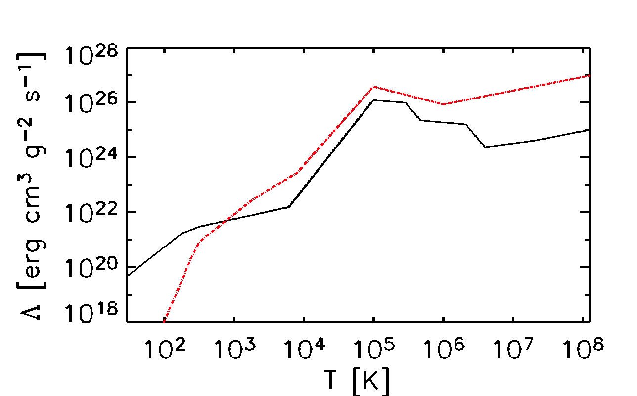
Figure 3.1: The cooling functions WSW (solid, black) and RB (red, dash-dotted), with parameters given in Tables 3.2 and 3.1, respectively.

I also include photoelectric heating in Eq. (3.1) via the stellar far-ultraviolet (UV) radiation $\Gamma$, following Wolfire et al. (1995), and allowing for its decline away from the Galactic mid-plane with a length scale comparable to the scale height of the stellar disc near the Sun (cf. Joung and Mac Low, 2006):

$$\Gamma(z)=\Gamma_{0}\exp\left(-|z|/300\,{\rm pc}\right),\quad\Gamma_{0}=0.0147\,{\rm erg}\,{\rm g}^{-1}\,{\rm s}^{-1}.$$

This heating mechanism is smoothly suppressed at $T>2\times 10^{4}\,{\rm K}$, since the photoelectric effect due to UV photon impact on PAHs (Polycyclic Aromatic Hydrocarbons) and small dust grains is impeded at high temperatures (Wolfire et al., 1995).

3.4 Numerical methods

The model occupies a relatively small region within the galactic disc and lower halo with parameters typical of the solar neighbourhood. Using a three-dimensional Cartesian grid, the results have been obtained for a region $1.024\times 1.024\times 2.240\,{\rm kpc}^{3}$ in size ($1.024\times 1.024\times 2.176\,{\rm kpc}^{3}$ for the MHD models), with $1.024\,{\rm kpc}$ in the radial and azimuthal directions and $1.120\,{\rm kpc}$ ($1.088\,{\rm kpc}$) vertically on either side of the galactic mid-plane. Assuming that the correlation length of the interstellar turbulence is $l_{0}\simeq 0.1\,{\rm kpc}$, it might be expected that the computational domain encompass about 2,000 turbulent cells, so the statistical properties of the ISM should be reliably captured. Testing individual SNe in diffuse ISM and snapshot sampling over various runs confirms the computational domain is sufficiently broad to accommodate comfortably even the largest SN remnants at large heights, so as to exclude any self-interaction of expanding remnants through the periodic boundaries.

Vertically, the reference model accommodates ten scale heights of the cold Hi gas, two scale heights of diffuse Hi (the Lockman layer), and one scale height of ionized hydrogen (the Reynolds layer). The vertical size of the domain in the reference model is insufficient to include the scale height of the hot gas and the Galactic halo. Therefore, it may be desirable to increase its vertical extent in future work. Note, however, that the size of SN remnants, and the correlation scale of the flow above a few hundred parsec height may approach the horizontal size of the numerical domain and may even exceed it at greater heights (Korpi, Brandenburg, Shukurov, Tuominen and Nordlund, 1999). The periodic boundary conditions exclude divergent flows at scales comparable to the horizontal size of the box, suggesting that an increase in height may necessitate an appropriate increase in the horizontal dimensions to reliably capture the dynamics of the flow, and remain consistent with the assumptions of the (sheared) periodic boundary conditions in $x$ and $y$.

The standard resolution (numerical grid spacing) is $\Delta x=\Delta y=\Delta z=\Delta=4\,{\rm pc}$. The grid is $256\times 256\times 560$ (excluding ’ghost’ boundary zones) for the HD models, slightly reduced to $256\times 256\times 544$ for the MHD models. One model at doubled resolution, $\Delta=2\,{\rm pc}$, has a grid $512\times 512\times 1120$ in size. A sixth-order finite difference scheme for spatial vector operations and a third-order Runge–Kutta scheme for time stepping are applied.

The spatial and temporal resolutions attainable impose lower limits on the kinematic viscosity $\nu$ and thermal conductivity $K$, which are, unavoidably, much higher than any realistic values. These limits result from the Courant–Friedrichs–Lewy (CFL) condition which requires that the numerical time step must be shorter than the crossing time over the mesh length $\Delta$ for each of the transport processes involved. It is desirable to avoid unnecessarily high viscosity and thermal diffusivity. The cold and warm phases have relatively small perturbation gas speeds (of order $10\,{\rm km\,s^{-1}}$), so $\nu$ and $\chi$ are prescribed to be proportional to the local speed of sound, $\nu=\nu_{1}c{{}_{\mathrm{s}}}/c_{1}$ and $\chi=\chi_{1}c{{}_{\mathrm{s}}}/c_{1}$. To ensure the maximum Reynolds and Péclet numbers based on the mesh separation $\Delta$ are always less than unity throughout the computational domain (see Appendix B.1), $\nu_{1}\approx 4.2\times 10^{-3}\,{\rm km\,s^{-1}}\,{\rm kpc}$, $\chi_{1}\approx 4.1\times 10^{-4}\,{\rm km\,s^{-1}}\,{\rm kpc}$ and $c_{1}=1\,{\rm km\,s^{-1}}$. This gives, for example, $\chi=0.019\,{\rm km\,s^{-1}}\,{\rm kpc}$ at $T=10^{5}\,{\rm K}$ and $0.6\,{\rm km\,s^{-1}}\,{\rm kpc}$ at $T=10^{8}\,{\rm K}$.

Numerical handling of the strong shocks widespread in the ISM needs special care. To ensure that they are always resolved, shock-capturing diffusion of heat, momentum and induction are included, with the diffusivities $\zeta_{\chi}$, $\zeta_{\nu}$ and $\zeta_{\eta}$, respectively, defined as

$$\zeta_{\chi}=\begin{cases}c_{\chi}\Delta x^{2}\max_{5}|\nabla\cdot{{\mbox{\boldmath$u$}}}|,&\text{if }\nabla\cdot{{\mbox{\boldmath$u$}}}<0,\\ 0,&\text{otherwise},\end{cases}$$ (3.9)

(and similarly for $\zeta_{\nu}$ or $\zeta_{\eta}$, but with coefficients $c_{\nu}$ or $c_{\eta}$), where ${\rm max_{5}}$ denotes the maximum value occurring at any of the five nearest mesh points (in each coordinate). Thus, shock-capturing diffusivity is proportional to the maximum divergence of the velocity in the local neighbourhood, and are confined to the regions of convergent flow. Here, $c_{\chi}=c_{\nu}=c_{\eta}$ is a dimensionless coefficient which has been adjusted empirically to 10. This prescription spreads a shock front over sufficiently many (usually, four) grid points. Detailed test simulations of an isolated expanding SN remnant in Appendix A confirm that this prescription produces quite accurate results, particularly in terms of the most important goal: the conversion of thermal to kinetic energy in SN remnants.

With a cooling function susceptible to thermal instability, thermal diffusivity $\chi$ has to be large enough as to allow us to resolve the most unstable normal modes:

$$\chi\geq\frac{1-\beta}{\gamma~{}\tau{{}_{\rm cool}}}\left(\frac{\Delta}{2\upi}\right)^{2},$$

where $\beta$ is the cooling function exponent in the thermally unstable range ($\beta=0.56$ in the WSW model), $\tau{{}_{\rm cool}}$ is the radiative cooling time, and $\gamma=5/3$ is the adiabatic index. From the contours of constant cooling time plotted in Fig. 7.1 of Chapter 7, it is evident that for these models $\tau{{}_{\rm cool}}$ is typically in excess of 1 Myr in the thermally unstable regime. Further details can be found in Appendix B.2 where it is demonstrated that, with the parameters chosen in my models, thermal instability is well resolved by the numerical grid.

The shock-capturing diffusion broadens the shocks and increases the spread of density around them. An undesirable effect of this is that the gas inside SN remnants cools faster than it should, thus reducing the maximum temperature and affecting the abundance of the hot phase. Having considered various approaches while modelling individual SN remnants in Appendix A, a prescription is adopted which is numerically stable, reduces gas cooling within SN remnants, and confines extreme cooling to the shock fronts. Specifically, the term $(\Gamma-\rho\Lambda)T^{-1}$ in Eq. (3.1) is multiplied by

$$\xi=\exp(-C|\nabla\zeta_{\chi}|^{2}),$$ (3.10)

where $\zeta_{\chi}$ is the shock diffusivity defined in Eq. (3.9). Thus $\xi\approx 1$ almost anywhere in the domain, but reduces towards zero in strong shocks, where $|\nabla\zeta_{\chi}|^{2}$ is large. The value of the additional empirical parameter, $C\approx 0.01$, was chosen to ensure numerical stability with minimum change to the basic physics. It has been verified that, acting together with other artificial diffusion terms, this does not prevent accurate modelling of individual SN remnants (see Appendix A for details).

3.5 Boundary conditions

Given the statistically homogeneous structure of the ISM in the horizontal directions at the scales of interest (neglecting arm-interarm variations), I apply periodic boundary conditions in the azimuthal ($y$) direction. Differential rotation is modelled using the shearing-sheet approximation with sliding periodic boundary conditions (Wisdom and Tremaine, 1988) in $x$, the local analogue of cylindrical radius.

Unlike the horizontal boundaries of the computational domain, where periodic or sliding-periodic boundary conditions may be adequate (within the constraints of the shearing box approximation), the boundary conditions at the top and bottom of the domain are more demanding. The vertical size of the galactic halo is of order of 10 kpc, and nontrivial physical processes occur even at that height, especially when galactic wind and cosmic ray escape are important. Within a few kiloparsecs of the mid-plane, SN heating induces a flow of hot gas towards the halo. The results of e.g., de Avillez and Breitschwerdt (2007, and references therein) suggest that in excess of $\pm 5\,{\rm kpc}$ is required for the hot gas to cool and return to the mid-plane. Their vertical extent ($z=\pm 10\,{\rm kpc}$) excludes significant mass loss from the system, but at considerable numerical expense. Because MHD runs may require simulation times exceeding 1 Gyr, it is desirable to restrict resources to the region, which can be reliably modelled with the minimum vertical extent. Gressel et al. (2008a) applied double the height modelled here, but with half the resolution, hence requiring a quarter of the resources. In adopting $\pm 1\,{\rm kpc}$ for the vertical boundary, there is no physical mechanism for adequate cooling and return of the hot gas, so care must be taken to address potential mass loss. For the HD runs, which require only a few Myr to acquire a statistically steady turbulent state, this is not too problematic. For the MHD runs mass must be replaced, and this is addressed in Appendix C.

It is also important to formulate boundary conditions at the top and bottom of the domain that admit the flow of matter and energy, while minimising any associated artefacts that might affect the interior. Stress-free, open vertical boundaries would seem to be the most appropriate, requiring that the horizontal stresses vanish, while gas density, entropy and vertical velocity have constant first derivatives on the top and bottom boundaries. These are implemented numerically using ‘ghost’ zones; i.e., three outer grid planes that allow derivatives at the boundary to be calculated in the same way as at interior grid points. The interior values of the variables are used to specify their ghost zone values.

Shocks occur ubiquitously within the ISM and handling these is particularly problematic as they approach the boundary. Within the computational domain and on the periodic boundaries, shocks are absorbed into the ambient medium, placing a finite limit on the magnitude of the momentum or energy associated with the shock. When a sharp structure approaches the vertical boundary, however, the strong gradients may be extrapolated into the ghost zones. This artificially enhances the prominence of such a structure, and may cause the code to crash. Here I describe how these boundary conditions have been modified to ensure the numerical stability of the model.

Mass

To prevent artificial mass sources in the ghost zones, I impose a weak negative gradient of gas density in the ghost zones. Thus, the density values are extrapolated to the ghost zones from the boundary point as

$$\rho(x,y,\pm Z\pm k\Delta)=(1-\Delta/0.1\,{\rm kpc})\rho(x,y,\pm Z\pm(k-1)\Delta)$$

for all values of the horizontal coordinates $x$ and $y$, where the boundary surfaces are at $z=\pm Z$, and the ghost zones are at $z=\pm Z\pm k\Delta$ with $k=1,2,3$. The upper (lower) sign is used at the top (bottom) boundary. This ensures that gas density gradually declines in the ghost zones.

Temperature

To prevent a similar artificial enhancement of temperature spikes in the ghost zones, gas temperature there is kept equal to its value at the boundary,

$$T(x,y,\pm Z\pm k\Delta)=T(x,y,\pm Z)\,,$$

so that temperature is still free to fluctuate in response to the interior processes. This prescription is implemented in terms of entropy, given the density variation described above.

Velocity

Likewise, the vertical velocity in the ghost zones is kept equal to its boundary value if the latter is directed outwards,

$$u_{z}(x,y,\pm Z\pm k\Delta)=u_{z}(x,y,\pm Z)\,,\qquad u_{z}(x,y,\pm Z)\gtrless 0\,.$$

However, when gas cools rapidly near the boundary, pressure can decrease and gas would flow inwards away from the boundary. To avoid suppressing inward flows, where

$$u_{z}(x,y,\pm Z)\lessgtr 0$$

the following is applied:

$${\textrm{if}}\quad|u_{z}(x,y,\pm Z\mp\Delta)|<|u_{z}(x,y,\pm Z)|,$$

set

$$u_{z}(x,y,\pm Z\pm\Delta)=\tfrac{1}{2}\left[u_{z}(x,y,\pm Z)+u_{z}(x,y,\pm Z\mp\Delta)\right]\,;$$

otherwise, set

$$u_{z}(x,y,\pm Z\pm\Delta)=2u_{z}(x,y,\pm Z)-u_{z}(x,y,\pm Z\mp\Delta)\,.$$

In both cases, in the two outer ghost zones ($k=2,3$), set

$$u_{z}(x,y,\pm Z\pm k\Delta)=2u_{z}(x,y,\pm Z\pm(k-1)\Delta)-u_{z}(x,y,\pm Z\pm(k-2)\Delta)\,,$$

so that the inward velocity in the ghost zones is always smaller than its boundary value. This permits gas flow across the boundary in both directions, but ensures that the flow is dominated by the interior dynamics, rather than by anything happening in the ghost zones.

For the horizontal components of the velocity at the vertical boundaries, symmetrical conditions are applied to exclude horizontal stresses, so

$$u_{x}(x,y,\pm Z\pm k\Delta)=u_{x}(x,y,\pm Z\mp k\Delta)\,,$$

and similarly for $u_{y}$.

Magnetic field

For the MHD models, two alternative sets of vertical boundary conditions are considered: vertical field and open. The objective with the vertical field condition is to exclude external flux. Any flux across the horizontal periodic boundaries conserves the magnetic energy. To identify a genuine dynamo process, the addition of magnetic energy due to non-physical boundary effects can be excluded by ensuring zero vertical flux on the upper and lower surfaces. For the horizontal components of the vector potential

$$A_{x}(x,y,\pm Z\pm k\Delta)=A_{x}(x,y,\pm Z\mp k\Delta)\,$$

and similarly for $A_{y}$, and for the vertical component

$$A_{z}(x,y,\pm Z\pm k\Delta)=-A_{z}(x,y,\pm Z\mp k\Delta)\,,$$

ensuring on the boundary that

$$\frac{\partial A_{x}}{\partial z}=\frac{\partial A_{y}}{\partial z}=A_{z}=0=B_{x}=B_{y}\,.$$

$B_{z}$ can differ from zero.

Such an approach creates a boundary layer, in which the non-zero horizontal fields near the surfaces, which may be significant close to $z\pm=1\,{\rm kpc}$, must vanish nonphysically.

The alternative open boundary conditions do not exclude external flux, but preserve the physical structure of the field up to the boundary. Gressel et al. (2008a) applied these with a domain up to $\pm 2\,{\rm kpc}$ in $z$, and argue the external magnetic flux was negligible. It is reasonable to expect, given the dominant flow of gas is outward in these simulations, that the outward magnetic flux might exceed the inward flux, so that artificial growth of the magnetic field due to boundary effects may be discounted. The vertical component of the Poynting flux on the boundary is monitored with these boundary conditions and the total flux outwards is 2 orders of magnitude greater than the total flux inwards. For the vertical component

$$A_{z}(x,y,\pm Z\pm k\Delta)=A_{z}(x,y,\pm Z\mp k\Delta)\,,$$

and for the horizontal components

$$A_{x}(x,y,\pm Z\pm k\Delta)=2A_{x}(x,y,\pm Z\pm(k-1)\Delta)-A_{x}(x,y,\pm Z\pm(k-2)\Delta)\,$$

and similar for $A_{y}$, such that

$$\frac{\partial^{2}A_{x}}{\partial z^{2}}=\frac{\partial^{2}A_{y}}{\partial z^{2}}=\frac{\partial A_{z}}{\partial z}=0=\frac{\partial B_{x}}{\partial z}=\frac{\partial B_{y}}{\partial z}\,.$$

The constraint on ${\partial B_{z}}/{\partial z}$ is automatically satisfied since $\nabla\cdot{{\mbox{\boldmath$B$}}}=0$.

3.6 Initial conditions

An initial density distribution is adopted corresponding to isothermal hydrostatic equilibrium in the gravity field of Eq. (3.7):

$$\rho(z)=\rho_{0}\exp\left[a_{1}\left(z_{1}-\sqrt{z_{1}^{2}+z^{2}}-\frac{a_{2}}{2a_{1}}\,\frac{z^{2}}{z_{1}}\right)\right].$$ (3.11)

Since some models do not contain magnetic fields and none contain cosmic rays, which provide roughly one quarter each of the total pressure in the ISM (the remainder being thermal and turbulent pressures), the gas scale heights can be expected to be smaller that those observed. Given the limited spatial resolution of the simulations, and the correspondingly weakened thermal instability and neglected self-gravity, it is not quite clear in advance whether the gas density used in the model should include molecular hydrogen or, otherwise, include only diffuse gas.

$\rho_{0}=3.5\times 10^{-24}\,{\rm g}\,{\rm cm^{-3}}$ is used for Models RBN and WSWb, corresponding to gas number density, $n_{0}=2.1\,{\rm cm^{-3}}$ at the mid-plane. This is the total interstellar gas density, including the part confined to molecular clouds. These models, discussed in Section 7.1, exhibit unrealistically strong cooling. Therefore, all other subsequent models have a smaller amount of matter in the computational domain (a 17% reduction), with $\rho_{0}=3.0\times 10^{-24}\,{\rm g}\,{\rm cm^{-3}}$, or $n_{0}=1.8\,{\rm cm^{-3}}$, accounting only for the atomic gas (see also Joung and Mac Low, 2006).

As soon as the simulation starts, because of density-dependent heating and cooling the gas is no longer isothermal, so $\rho(z)$ given in Eq. (3.11) is not a hydrostatic distribution. To avoid unnecessarily long initial transients, a non-uniform initial temperature distribution is imposed so as to be near static equilibrium:

$$T(z)=\frac{T_{0}}{z_{1}}\left(\sqrt{z_{1}^{2}+z^{2}}+\frac{a_{2}}{2a_{1}}\frac{z^{2}}{z_{2}}\right),$$ (3.12)

where $T_{0}$ is obtained from

$$\Gamma(0)=\rho_{0}\Lambda(T_{0})\approx 0.0147\,{\rm erg}\,{\rm g}^{-1}\,{\rm s}^{-1}.$$

The value of $T_{0}$ therefore depends on $\rho_{0}$ and the choice of the cooling function.

For the models that include a magnetic field, the initial seed field ${{\mbox{\boldmath$B$}}}=(0,B_{I}n(z),0)$. I use $B_{I}=0.05\,\umu{\rm G}\,{\rm cm}^{3}$ and $n_{0}=1.8\,{\rm cm^{-3}}$, such that ${\langle B{{}_{\rm rms}}\rangle}\simeq 0.001\,\umu{\rm G}$ with ${\langle\cdot\rangle}$ indicating the average over the computational domain.

Due to differential cooling and heating in the vertically stratified gas the initial setup is in an unstable equilibrium, resulting in collapse and subsequent oscillations. A new equilibrium requires the gradual build up of thermal and turbulent pressure, followed by an extended period while the oscillations of the disc dissipate and the disc becomes statistically steady. Gressel et al. (2008b) eliminate these transients by adjusting the vertical heating profile to balance exactly the initial cooling. While heating may be only marginal to the long term dynamics of the model, this does add a long term unphysical ingredient. An alternative approach, for future reference, may be to begin without heating and cooling in isothermal, hydrostatic equilibrium. This would be a stable equilibrium, and the heating and cooling terms could be switched on after the thermal and turbulent pressures are sufficiently developed to support the gas against gravitational collapse. This may reduce the duration, and hence numerical expense, of the initial transients.

3.7 Simulation vs. ’realised’ time, and geometry

For this model, as with other models of this type, the unperturbed initial conditions, which cannot be expected to exist in nature, require an extended period of simulation time to reach a quasi-steady turbulent state. Joung and Mac Low (2006) allow 40 Myr for the initial transients to be subsumed by turbulence, while using a similar model de Avillez and Breitschwerdt (2007) argue this should be more like 200 Myr. The initial conditions are not in equilibrium due to the heating and cooling terms, and in the absence of thermal stability there is a large scale collapse of the disc. The thickness of the disc is gradually expanded by the build up of both thermal and ram pressure by the injection of SNe. There remain large scale vertical oscillations from the initial collapse, which require longer to settle. In my model the regular systematic oscillations dissipate over a timescale of at least 100 Myr, but not more than 200 Myr, although random fluctuations occur at later times.

The quasi-steady turbulent state then needs to be tracked over a few hundred Myr to provide reliable statistics for a robust analysis. For models tracing the galactic dynamo, with the relatively low magnetic Reynolds numbers available in the model, it is necessary to run them for up to 2 Gyr to see the magnetic field grow to saturation. Is it then reasonable to assume that the models have a time independent statistically steady state? Tutukov, Shustov and Wiebe (2000) model the lifetime evolution of the Galaxy. They suggest significant variation of star formation and SN rates occur in timescales of a few hundred Myr, with associated changes to the ISM mass and thickness of the disc. On the scale of 1 Gyr, qualitative as well as quantitative effects might be expected to occur. These scales are based on highly simplified premises and are only indicative of galactic trends. Nevertheless it is reasonable to question whether a steady hydrodynamical state should persist over such long timescales.

Consider also the effect of time on the geometry of the numerical domain. Nominally the box is differentially rotating around the Galactic centre. Due to the differential rotation in the azimuthal direction the boundary nearest to the galactic centre moves ahead of the corresponding outer boundary, and this is realised in the model by the sliding periodic boundary conditions. The numerical domain therefore is elongated in the azimuthal direction over time as illustrated in Fig. 3.2. The rectangular box in the bottom left follows the orbit about the galactic centre, being increasingly distorted as shown. If we regard the sliding boundaries to be forever moving apart in this way, as the simulation box completes several orbits, the geometry would rapidly cease to resemble a rectangle and be stretched much like an elastic band.

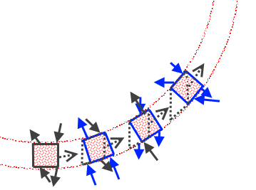
Figure 3.2: Illustration of the preservation of horizontal geometry of the simulation domain using the shearing box approximation. An arbitrary starting location for the orbit of the numerical box about the galactic centre is indicated by the rectangular box bottom left. Differential rotation is represented by the inner boundary moving ahead of the outer ($2^{\rm nd}$ position). The dotted arrows denote the angular velocity of the box. The rectangular geometry of the box is maintained by substituting statistically identical gas in the blue triangle ahead of the box for the gas in the trailing grey triangle. Arbitrary positions on the outer boundary subject to some velocity, are indicated by the solid arrows, grey arrows for an original section and blue for a section of the substituted edge and its substitute. Corresponding arrows on the inner boundary indicate the offset postitions. The offset from the original edge increases, while the offset from the substitute edge decreases ($3^{\rm rd}$ position). By the time the sliding boundaries have been offset by their full length ($4^{\rm th}$ position) the inner and outer edges are in exact correspondence. Thus the blue rectangle in the $4^{\rm th}$ postion becomes a new arbitrary starting postion and the process repeats.

However to first approximation let us suppose the ISM in the neighbourhood of our box in the horizontal directions to be statistically homogeneous to that within the box. Consider the position of the $2^{\rm nd}$ box in Fig. 3.2, with the inner boundary in advance of the outer, illustrated by dotted grey lines. Statistically there is little to distinguish gas within the triangular region bounded by the rear blue edge and the trailing corner from that bounded by the leading and outer blue edges and leading dotted line. Preserving the geometry of the box (blue) as it orbits the galaxy, gas in the trailing triangle is replaced by equivalent gas occupying an identical region of the ISM previously just ahead of the box. Some typical flow, denoted by the solid blue arrows, identifies the identical conditions on the trailing and substitute gas near the outer edge, and the corresponding position on the inner edge ($2^{\rm nd}$ and $3^{\rm rd}$ positions). The solid grey arrows denote such flow across original sections. The offset between the black arrows increases with the shear, and the offset between the blue arrows reduces, until the offset for the original edges is the full length of the boundary ($4^{\rm th}$ position). At this point the inner and outer edges are no longer offset and the process is repeated from this new starting geometry (indistinguishable from the $1^{\rm st}$ position).

With respect to the time, the total simulation time might be considered independent of the physical time to which it is scaled. Only the physical processes inside the calculation are actually tracking real time. Supernova remnants, the advection time of the hot gas from the disc to the boundary, the life times of superbubbles containing multiple SNe have simulation times matching the corresponding physical times. The superbubbles have the longest duration of all the locally coherent physical features in the simulation domain. The premise of the periodic boundary conditions is that horizontally the properties of the ISM in the neighbourhood are statistically identical to first approximation. Thus as one superbubble dissipates and a new one evolves, rather than regarding the new event as occurring later in time it is reasonable to regard it as occurring at the same time in some random location in the neighbourhood. From this conception the entire simulation can be regarded as occurring simultaneously in the quasi-steady state, whose physical time frame need only match the simulation time of the longest lasting superbubble.

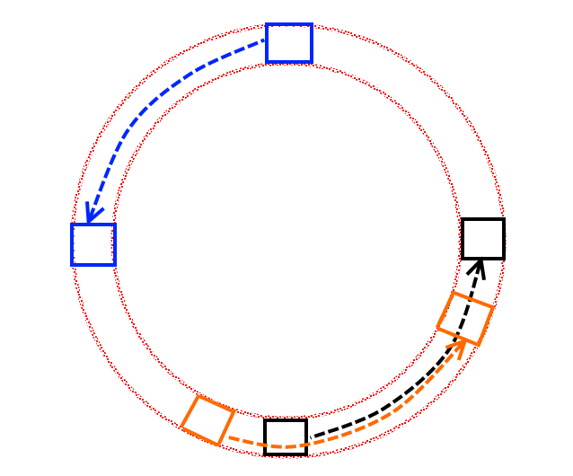
Figure 3.3: Illustration of the distinction between simulation time and realised time, as explained in the text.

In Fig. 3.3 this principle is illustrated. Consider an arbitrary starting time for the simulation in the statistically steady state to correspond to the initial position of the black box. It orbits for 60–100 Myr as shown. The simulation continues, but could be considered now to be modelling an entirely different part of the orbit, shown in blue, but regarded in the realised time frame to be concurrent with the part just modelled in black. Hence, 120–200 Myr of simulation time has elapsed, but only 60–100 Myr of realised time need be considered to have elapsed. Given the statistical homogeneity of the ISM within the neighbourhood of the orbit, even a nearby parcel of ISM, indicated by the orange box, could be regarded as statistically independent of the original sample. In this way each segment of 60–100 Myr may be considered as repeated sampling of the independent sections of the ISM in the same orbit over the same time period, irrespective of how long the simulation lasts. Similarly, the extended simulation time may be considered in terms of ensemble sampling from appropriate neighbourhoods within multiple galaxies, where the common parameters apply.

The only feature that is modelled here that has a structure larger than the local box, and evolves over time scales exceeding the longest lasting superbubbles, is the mean magnetic field. However, the large scale structure of the mean field, is in reality also a statistical property of the random magnetic field on the local scale. Rather than single field lines extending azimuthally over kpc scales, the field lines are highly scattered, but with a preferential orientation in the direction of shear. The large scale organization of the field in the model is therefore not due to any physical superstructures, but to alignment within the random small scale structures.

Finally, the large time scales required to follow the growth of the magnetic dynamo may contravene the assumption of a quasi-steady state. In this case the magnetic Reynolds numbers in the simulations are far smaller than in the real ISM, so it may be expected that the growth rates would be much slower in the simulations. Also here, however, it would be an error to regard the tracing of the dynamo as a physically continuous process. Instead, the appropriate interpretation of time in the dynamo runs, is that each 100–300 Myr of the simulation represents statistical sampling of hydrodynamically similar galaxies with magnetic fields at various stages of maturity.

Chapter 4 Models explored

4.1 Summary of models

I consider five numerical models which do not include magnetic fields (HD), and five which do (MHD), and these are named in Table 4.1 Column 1, together with some of the more important input parameters. Some significant statistical outcomes describing the results for each model are displayed in Table 4.2. The HD models are labelled with prefix RBN or WSW to denote the cooling function used (as described in Section 3.3). All the MHD models use the WSW cooling function, so WSW is dropped and labels identify the other key parameters applied.

Table 4.1: Selected input parameters of the numerical models explored in this paper, named in Column (1). Column: (2) numerical resolution; (3) galactic rotation rate $\Omega$; (4) galactic shear rate $S$; (5) galactic supernovae rate $\dot{\sigma}$; (6) initial mid-plane gas number density $n_{0}$; (7) magnetic field $B$; (8) vertical boundary condition on magnetic potential $A$ (Sect. 3.1); (9) Section where particular model is considered. The estimates for the solar neighbourhood of mean angular velocity $\Omega_{0}$ and rate of SN explosions $\dot{\sigma}_{0}$ (Sect. 3.1 and 3.2).

(1)	(2)	(3)	(4)	(5)	(6)	(7)	(8)	(9)
Model	$\Delta$	$\Omega$	$S$	$\dot{\sigma}$	$n_{0}$	${{\mbox{\boldmath$B$}}}\neq{{\mbox{\boldmath$0$}}}$	bc$z({{\mbox{\boldmath$A$}}})$	Section
	[pc]	$[\Omega_{0}]$	$[\Omega_{0}]$	$[\dot{\sigma}_{0}]$	[$\!\,{\rm cm^{-3}}$]
WSWa	4	1	-1	1	1.8	no	–	5, 6, B.2
WSWah	2	1	-1	1	1.8	no	–	5.1
RBN	4	1	-1	1	2.1	no	–	7.1, C
WSWb	4	1	-1	1	2.1	no	–	7.1, C
${\mathrm{H}1\rm{\Omega}}$	4	1	-1	1	1.8	no	–	7.2, 9
${\mathrm{B}1\rm{\Omega}}$	4	1	-1	1	1.8	yes	vertical	7.1, 9
${\mathrm{B}1\rm{\Omega}\rm{O}}$	4	1	-1	1	1.8	yes	open	9
${\mathrm{B}2\rm{\Omega}}$	4	2	-2	1	1.8	yes	vertical	8, 9, C
${\mathrm{B}1\rm{\Omega}\rm{SN}}$	4	1	-1	0.8	1.8	yes	vertical	7.2, 9
${\mathrm{B}1\rm{\Omega}\rm{Sh}}$	4	1	-1.6	1	1.8	yes	vertical	7.2, 9

For the MHD models, ${\mathrm{B}1\rm{\Omega}}$ and ${\mathrm{B}1\rm{\Omega}\rm{O}}$ denote models with parameters matching the solar neighbourhood, but with alternative vertical boundary conditions, as described in Section 3.5; all models (HD also) have a rate and distribution of supernova explosions equivalent to the solar neighbourhood estimates $\dot{\sigma}_{0}$, as explained in Section 3.2, except for ${\mathrm{B}1\rm{\Omega}\rm{SN}}$ at $0.8\dot{\sigma}_{0}$; ${\mathrm{B}2\rm{\Omega}}$ has galactic rotation $\Omega$ and shearing $-S$ double the value $\Omega_{0}=25\,{\rm km\,s^{-1}}\,{\rm kpc}^{-1}$ introduced in Section 3.1; and ${\mathrm{B}1\rm{\Omega}\rm{Sh}}$ has a shearing rate $-1.6\Omega_{0}$. The primary motivation for these variations is to investigate the sensitivity of the dynamo to the parameters.

Some adjustments to the model are implemented for the MHD runs, to stabilize the disc and to recycle mass, which is transported across the vertical boundaries over the extended duration required for the dynamo. These are detailed in Appendix C. To assist direct comparison with the HD models, Model WSWa is repeated with these adjustments applied, and labelled in Table 4.1 as ${\mathrm{H}1\rm{\Omega}}$.

Column 2 of Table 4.1 lists the resolution applied in each model. The standard resolution is $(4\,{\rm pc})^{3}$, with only one model, WSWah, having $(2\,{\rm pc})^{3}$. The latter model is applied to assess the sensitivity of the models to resolution. The starting state for this model is obtained by remapping a snapshot at $t=600$ Myr from the standard-resolution Model WSWa (when the system has settled to a statistically steady state) onto a grid $512\times 512\times 1120$ in size. Resolutions of $(1\,{\rm pc})^{3}$, $(2\,{\rm pc})^{3}$ and $(4\,{\rm pc})^{3}$ were tested for separate analysis of single remnant models in uniform monotonic ambient ISM of various densities (see Appendix A.1), prior to conducting these comprehensive simulations.

The initial conditions, described in Section 3.6, are intended to be transient, with the statistically steady state into which the models evolve being independent of the initial state within 2–4 Myr of the start. Subsequent evolution however is not independent of the initial density profile, and to facilitate comparison of my results with theory and observations, it is important that the density profile in the evolved state should be close to the estimated values for the solar neighbourhood. In the HD models, we would expect the combined thermal and RAM pressure supporting the gas against gravitational acceleration to be weaker than the observed ISM, due to the absence of magnetic and cosmic ray pressure. Cosmic ray pressure is absent from all models. Since the model resolution does not resolve the dense molecular clouds, it is not clear in advance whether to include this contribution to the ISM density. Models RBN and WSWb  are initialised with the contribution from molecular hydrogen included, while all other models exclude it, as listed in Column 6.

The parameters of rotation, shear and supernova rate are listed in Columns 3, 4 and 5 of Table 4.1. Column 7 indicates whether a magnetic field is included, and Column 8 indicates which boundary conditions apply to the vector potential $A$ on the upper and lower surfaces, which are described in Section 3.5. Column 9 lists the Sections of this thesis in which the results for each model are described.

These models are computationally demanding. The standard resolution models require parallel processing on around 280 nodes and consume around 100 000 cpu hours for 100 Myr of simulation. Therefore, to maximise the results from the available resources, only three models have been run from the initial conditions at $t=0$ yr. These were Models RBN, WSWb  and ${\mathrm{B}1\rm{\Omega}}$, which were evolved until the systems were in the hydrodynamical steady turbulent state, at about 200 Myr, and then continued to at least 600 Myr.

Model WSWa  was initialised from a turbulent snapshot of WSWb  at 400 Myr, but had the gas density at every point reduced by about 17%, so that the revised density profile corresponded to the estimated rates for the solar neighbourhood, excluding molecular hydrogen. It was then continued to 675 Myr, sufficient for any transients arising from the adjustment to subside. Model WSWah  was initialised by remeshing a snapshot from Model WSWa  at about 600 Myr, and was continued to 650 Myr. Due to the reduced grid spacing and the improved resolution of gradients in all variables, the iterative time step reduces substantially to satisfy the Courant-Friedrichs-Lewy (CFL) condition. The impact is an increase of 10–30 times in the computational demands to advance the simulation each Myr. Consequently, only about 50 Myr were completed for this model, which may perhaps yield insufficient statistics for the steady state of this simulation.

For the magnetic runs, ${\mathrm{B}1\rm{\Omega}}$ was run to 400 Myr, and then all of these models were continued from this snapshot with the revised parameters as listed in Table 4.1. It becomes apparent from the rates of growth that if the dynamo is successful, it would require in excess of 2 Gyr for the magnetic field to grow to saturation. Each is run for another several hundred Myr, enough to identify the presence of a dynamo and provide a basis for comparisons between the models. To investigate the dynamo process to saturation, Model ${\mathrm{B}2\rm{\Omega}}$, with the fastest growing dynamo, is continued to 1.7 Gyr. The dynamo saturates at about 1.1 Gyr and then continues with the system in a statistically steady state. For comparisons in the saturated regime, models ${\mathrm{B}1\rm{\Omega}\rm{O}}$ and ${\mathrm{B}1\rm{\Omega}}$ are restarted from a snapshot of ${\mathrm{B}2\rm{\Omega}}$ at 1.2 Gyr and 1.4 Gyr respectively, and continued for a further 400 Myr each.

4.2 Model data summary

Table 4.2: Column (1) lists the models from Table 4.1 with some indicative results: (10) average sound speed ${\langle c{{}_{\mathrm{s}}}\rangle}$; (11) average kinematic viscosity ${\langle\nu\rangle}$; (12) average Reynolds number defined at the grid spacing $\langle{\rm Re}_{{}_{\Delta}}\rangle$; (13) average r.m.s. perturbation velocity ${\langle u{{}_{\rm rms}}\rangle}$; (14) turbulent velocity ${\langle u_{\rm turb}\rangle}$; (15) thermal energy density ${\langle e_{\mathrm{th}}\rangle}$; (16) kinetic energy density ${\langle e_{\mathrm{kin}}\rangle}$; (17) magnetic energy density ${\langle e_{\mathrm{B}}\rangle}$; and (18) time span over which the models have been in steady state ($\tau$ is the typical horizontal crossing time); Standard deviation over volume using eleven composite snapshots (ten for WSWah) per model are given in brackets.

(1)	(10)	(11)	(12)	(13)	(14)	(15)	(16)	(17)	(18)
Model	${\langle c{{}_{\mathrm{s}}}\rangle}$	${\langle\nu\rangle}$	${\langle{\rm Re}_{{}_{\Delta}}\rangle}$	${\langle u{{}_{\rm rms}}\rangle}$	${\langle u_{\rm turb}\rangle}$	${\langle e_{\rm th}\rangle}$	${\langle e_{\rm kin}\rangle}$	${\langle e_{\rm B}\rangle}$	$\Delta t$
	$[\!\,{\rm km\,s^{-1}}]$			$[\!\,{\rm km\,s^{-1}}]$	$[\!\,{\rm km\,s^{-1}}]$	[$E_{\rm SN}\,{\rm kpc}^{-3}$]	[$E_{\rm SN}\,{\rm kpc}^{-3}$]	[$E_{\rm SN}\,{\rm kpc}^{-3}$]	[$\tau$]
WSWa	$108~{}(113)$	$0.44$	$0.88$	$\phantom{1}76~{}{\phantom{0}}(85)$	$26~{}(27)$	$30~{}{\phantom{0}}(87)$	$13~{}(34)$	–	3.9
WSWah	$186~{}(207)$	$0.77$	$0.85$	$103~{}(124)$	$34~{}(37)$	$19~{}{\phantom{0}}(59)$	$10~{}(50)$	–	0.5
RBN	$\phantom{2}58~{}(118)$	$0.24$	$1.18$	$\phantom{1}37~{}{\phantom{0}}(42)$	$18~{}(22)$	$25~{}(115)$	${\phantom{0}}9~{}(25)$	–	2.7
WSWb	$\phantom{2}65~{}{\phantom{0}}(75)$	$0.27$	$0.97$	$\phantom{1}45~{}{\phantom{0}}(49)$	$20~{}(22)$	$29~{}{\phantom{0}}(85)$	$13~{}(46)$	–	4.0
${\mathrm{B}1\rm{\Omega}}$	${\phantom{0}}23~{}{\phantom{0}}(25)$	$0.09$	$0.64$	${\phantom{0}}12~{}{\phantom{0}}(11)$	${\phantom{0}}5~{}{\phantom{0}}(6)$	$25~{}{\phantom{0}}(93)$	${\phantom{0}}5~{}(13)$	$5{\phantom{0.}}~{}{\phantom{0.}}(8)$	1.5
${\mathrm{B}1\rm{\Omega}\rm{O}}$	${\phantom{0}}23~{}{\phantom{0}}(22)$	$0.09$	$0.65$	${\phantom{0}}13~{}{\phantom{0}}(14)$	${\phantom{0}}6~{}{\phantom{0}}(8)$	$25~{}{\phantom{0}}(96)$	${\phantom{0}}6~{}(15)$	$3{\phantom{0.}}~{}{\phantom{0.}}(5)$	1.9
${\mathrm{B}2\rm{\Omega}}$	${\phantom{0}}21~{}{\phantom{0}}(21)$	$0.09$	$0.59$	${\phantom{0}}11~{}{\phantom{0}}{\phantom{0}}(9)$	${\phantom{0}}5~{}{\phantom{0}}(6)$	$26~{}(102)$	${\phantom{0}}5~{}(15)$	$7{\phantom{0}}~{}{\phantom{0}}(10)$	2.0
${\mathrm{H}1\rm{\Omega}}$	${\phantom{0}}41~{}{\phantom{0}}(65)$	$0.17$	$0.95$	${\phantom{0}}33~{}{\phantom{0}}(45)$	$12~{}(16)$	$26~{}{\phantom{0}}(74)$	${\phantom{0}}9~{}(19)$		4.8
${\mathrm{B}1\rm{\Omega}}^{*}$	${\phantom{0}}58~{}{\phantom{0}}(75)$	$0.24$	$0.88$	${\phantom{0}}38~{}{\phantom{0}}(47)$	$15~{}(19)$	$25~{}{\phantom{0}}(66)$	$10~{}(26)$	$0.1~{}(0.4)$	4.5
${\mathrm{B}1\rm{\Omega}\rm{SN}}$	${\phantom{0}}21~{}{\phantom{0}}(23)$	$0.09$	$1.01$	${\phantom{0}}18~{}{\phantom{0}}(13)$	${\phantom{0}}6~{}{\phantom{0}}(8)$	$23~{}{\phantom{0}}(75)$	${\phantom{0}}7~{}(16)$	$0.1~{}(0.4)$	2.5
${\mathrm{B}1\rm{\Omega}\rm{Sh}}$	${\phantom{0}}24~{}{\phantom{0}}(32)$	$0.10$	$0.96$	${\phantom{0}}20~{}{\phantom{0}}(18)$	${\phantom{0}}7~{}(10)$	$29~{}{\phantom{0}}(94)$	${\phantom{0}}7~{}(24)$	$0.1~{}(0.4)$	3.6

In Table 4.2 some indicative data from the various models identified in Table 4.1 are displayed. Here angular brackets denote averages over the whole volume, taken from eleven snapshots (10 for WSWah) within the statistical steady state. The standard deviations (in brackets) are spatial fluctuations for the combined snapshots. The time span, $\Delta t$, is given in Column 18, normalised by $\tau=L_{x}/{\langle u_{\rm turb}\rangle}$, where $u_{\rm turb}$ is the root-mean-square random velocity and $L_{x}\approx 1\,{\rm kpc}$ is the horizontal size of the computational domain. For the HD models, this refers to the steady state. For the MHD models the system has been in a hydrodynamically steady state much longer than the $\Delta t$ as listed. For ${\mathrm{B}1\rm{\Omega}}$, ${\mathrm{B}1\rm{\Omega}\rm{O}}$ and ${\mathrm{B}2\rm{\Omega}}$, $\Delta t$ refers to the latter period when the magnetic field is also in a statistical steady state. For ${\mathrm{B}1\rm{\Omega}\rm{SN}}$ and ${\mathrm{B}1\rm{\Omega}\rm{Sh}}$, the field is still growing and $\Delta t$ refers only to how long the system has been hydrodynamically steady. Results are also taken from Model ${\mathrm{B}1\rm{\Omega}}$ during the kinematic stage, for comparison with the latter models; these are listed in the table as ${\mathrm{B}1\rm{\Omega}}^{*}$. As $\nu$ is set proportional to the speed of sound $c{{}_{\mathrm{s}}}$ (Column 10) it is variable, and the table presents its average value ${\langle\nu\rangle}=\nu_{1}{\langle c{{}_{\mathrm{s}}}\rangle}$ as Column 11, where $\nu_{1}=0.004$ in all models.

The numerical resolution is sufficient when the mesh Reynolds number, ${\rm Re}{{}_{\Delta}}=u\,{\Delta}/\nu$, does not exceed a certain value (typically between 1 and 10) anywhere in the domain. The indicative parameter values of the mesh Reynolds number in Table 4.2 Column 12 are averages, $\langle{\rm Re}{{}_{\Delta}}\rangle={\Delta}{\langle u_{\rm turb}/c{{}_{\mathrm{s}}}\rangle}/\nu_{1}$, where ${\Delta}$ is the grid spacing (4 pc for all models, except for Model WSWah, where ${\Delta}=2\,{\rm pc}$). Although ${\rm Re}{{}_{\Delta}}$ is typically close to 1 in all models, for some locations this could be much greater. However, $u\,{\Delta}/\nu<5$, is ensured through the combination of temperature dependent bulk diffusion and shock enhanced diffusion.

Other quantities shown in Table 4.2 have been calculated as follows. In Column 13 ${\langle u{{}_{\rm rms}}\rangle}$ is derived from the total perturbation velocity field $u$, which excludes only the overall galactic rotation $U$. In Column 14 ${\langle u_{\rm turb}\rangle}$ is obtained from the turbulent velocity only, with the mean flows ${\langle{{\mbox{\boldmath$u$}}}\rangle}_{\ell}$, defined in Eq. (3.6), deducted from $u$. In Columns 15 and 16, $e_{\mathrm{th}}=\langle\rho e\rangle$ and $e_{\mathrm{kin}}=\langle\tfrac{1}{2}\rho u^{2}\rangle$ are the average thermal and kinetic energy densities respectively; the latter includes the perturbed velocity $u$, and both are normalised by the SN energy $E_{\rm SN}=10^{51}\,{\rm erg}$. In Column 17 $e_{\mathrm{B}}={\langle B^{2}/8\upi\rangle}$ is the average magnetic energy density, also normalised by $E_{\rm SN}$. For the magnetic runs, the energies are given for the stage after the magnetic field has saturated, except for Models ${\mathrm{B}1\rm{\Omega}\rm{SN}}$, ${\mathrm{B}1\rm{\Omega}\rm{Sh}}$ and ${\mathrm{B}1\rm{\Omega}}^{*}$, for which data is only available for the kinematic stage.

Part III Multiphase description of the interstellar medium

Chapter 5 Is the ISM multi-phase?

As explained in Section 1.2.2 the ISM has been described as comprising dynamically distinct regions of hot, warm and cold gas (Cox and Smith, 1974; McKee and Ostriker, 1977), which co-exist in relative pressure equilibrium. This was postulated theoretically; due to differential cooling rates of the gas at various states (temperature and density composition, which here I shall refer to as phases) compared to the rate of thermal conductivity in the ISM, it could be expected that the phases would settle to pressure equilibrium far faster than they diffuse into a thermal equilibrium. Since observations confirm gas exists at temperatures typical of the cold at $T\simeq 10^{2}\,{\rm K}$, warm at $T\simeq 10^{4}\,{\rm K}$ and hot at $T\simeq 10^{6}\,{\rm K}$ this picture of phases in pressure balance would appear to be inevitable.

However the description becomes less convincing once the highly turbulent nature of the ISM is considered. The continual shocks and heating produced by SNe create bubbles of extremely hot gas surrounded by ballistically propelled cold dense shells. It cannot be excluded that in fact these phases are merely transitory features of a violently perturbed medium with a broad spectrum of randomly distributed pressures, where gases of different temperatures merely occupy part of the continuum of a qualitatively homogeneous gas (V09, discussion on The controversy).

In this chapter I report how my results address this issue using the model which most closely resembles the Milky Way, WSWa. The observational data and our understanding of the ISM is strongest for the solar neighbourhood and this also provides a good basis for assessing the accuracy of my model. If a distinction between the phases can be justified it may be useful in interpreting observations. Trying to make sense of observations and statistical inferences from data, with such huge scale separation of 6 to 10 orders of magnitude, is highly unreliable. If separation into phases is valid then it permits observers and theoreticians to make inferences on more discrete data sets, with better defined characteristics in terms of for example mass, velocity, temperature and magnetic field distributions.

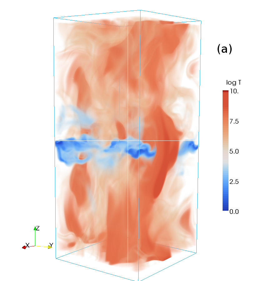
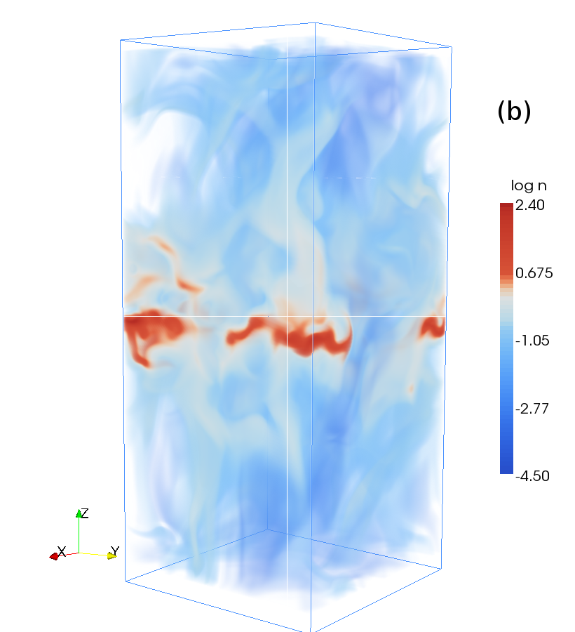
Figure 5.1: A three-dimensional rendering of (a) temperature and (b) density distributions in Model WSWa at $t=551\,{\rm Myr}$. Cold, dense gas is mostly located near the mid-plane, whereas hot gas extends towards the upper and lower boundaries. To facilitate visualisation of the 3D structure, warm gas ($10^{3}<T<10^{6}\,{\rm K}$) and diffuse gas ($n<10^{-2}\,{\rm cm}^{-3}$) are plotted with high transparency, so that extreme temperatures, and dense structures are emphasized.

Model WSWa is taken as a hydrodynamic (HD) reference model, because it has rotation corresponding to a flat rotation curve with the Solar angular velocity, and gas density comparable to the solar neighbourhood, but excluding the molecular clouds (See Appendix C for a discussion of the effect of this change of total mass).

Figure 5.1 shows typical temperature and density distributions at $t=551\,{\rm Myr}$ (i.e., $151\,{\rm Myr}$ from the start of run WSWa). Supernova remnants appear as irregularly shaped regions of hot, dilute gas. A hot bubble breaking through the cold gas layer extends from the mid-plane towards the lower boundary, visible as a vertically stretched region in the temperature snapshot near the $(x,z)$-face. Another, smaller bubble can be seen below the mid-plane near the $(y,z)$-face. Cold, dense structures are restricted to the mid-plane and occupy a small part of the volume. Very hot and cold regions exist in close proximity.

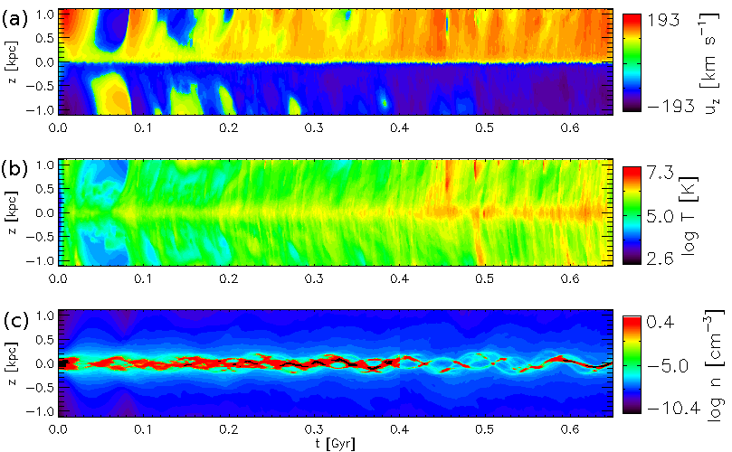
Figure 5.2: Horizontal averages of (a) the vertical velocity, (b) temperature and (c) gas density as functions of time for Model WSWa (Model WSWb up to 0.4 Gyr).

Horizontally averaged quantities, as functions of height and time, are plotted in Fig. 5.2 for Model WSWb at $t<400\,{\rm Myr}$, and WSWa at later times, showing the effect of reducing the total mass of gas at the transition time. This figure shows the vertical velocity (panel a), temperature (b) and gas density (c). Average quantities may have limited physical significance, because the multi-phase gas structure encompasses an extremely wide range of conditions. For example panel (b) shows that the average temperature near the mid-plane, $|z|\,\hbox to0.0pt{\raise 2.15277pt\hbox{$<$}\hss}{\lower 4.30554pt\hbox{$\sim$}}\,0.35\,{\rm pc}$, is, perhaps unexpectedly, generally higher than that at the larger heights. This is due to SN II remnants, which contain very hot gas with $T\,\hbox to0.0pt{\raise 2.15277pt\hbox{$>$}\hss}{\lower 4.30554pt\hbox{$\sim$}}\,10^{8}\,{\rm K}$ and are concentrated near the mid-plane; even though their total volume is small, they significantly affect the average temperature.

Nevertheless these average conditions help to illustrate some global properties of the simulations. Before the system settles into a quasi-stationary state at about $t=250\,{\rm Myr}$, it undergoes a few large-scale transient oscillations involving quasi-periodic vertical motions. The periodicity of approximately 100 Myr, is consistent with the breathing modes identified by Walters and Cox (2001) in 1D models with vertical perturbations, attributable to the gravitational acceleration. Gas falling from altitude will pass through the mid-plane, where the net vertical gravity is zero and so continues its trajectory until the increasing gravity with height again reverses it. Turbulent pressure and gas viscosity dampen these modes. At later times, a systematic outflow develops with an average speed of about $100\,{\rm km\,s^{-1}}$; we note that the vertical velocity increases very rapidly near the mid-plane and varies much less at larger heights. The result of the reduction of gas density at $t\approx 400\,{\rm Myr}$ is clearly visible, as it leads to higher mean temperatures and a stronger and more regular outflow, together with a less pronounced and more disturbed layer of cold gas.

5.1 Identification of a multi-phase structure

All models described in this thesis, including the HD reference Model WSWa, have a well-developed multi-phase structure apparently similar to that observed in the ISM. Since the ISM phases are not genuine, thermodynamically distinct phases (V09), their definition is tentative, with the typical temperatures of the cold, warm and hot phases usually set at $T\simeq 10^{2}\,{\rm K}$, $10^{4}$–$10^{5}\,{\rm K}$ and $10^{6}\,{\rm K}$, respectively.

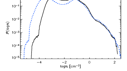
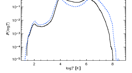
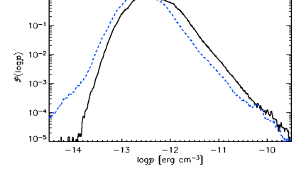
Figure 5.3: Volume weighted probability distributions of gas number density (a), temperature (b) and thermal pressure (c) for models WSWa (black, solid) and WSWah (blue, dashed) for the total numerical domain $|z|\leq 1.12\,{\rm kpc}$.

From inspection of the total volume probability density distributions shown in Fig. 5.3 it is not necessarily apparent that such a description is justified. The black solid lines refer to Model WSWa and the blue dashed lines refer to Model WSWah, which differs only in its doubly enhanced resolution and against which the sensitivity to resolution may be measured. In panel (b) there are clearly three distinct peaks in the temperature, corresponding roughly to the conventional definitions. For the gas density and temperature probability distributions (Fig. 5.3a and b) the minima in the distributions appear independent of resolution (at density $10^{-2}\,{\rm cm}^{-3}$, and at temperatures $10^{2}$ and $3\times 10^{5}$ K). The distributions are most consistent in the thermally unstable range 313 – 6102 K. The minimum about the unstable range above $10^{5}\,{\rm K}$ is more pronounced with the higher resolution, because the hotter gas has reduced losses to thermal conduction. The modal temperatures of the cold gas ($100$ K) and warm gas ($10^{4}$ K) are consistent. In Fig. 5.3 for Model WSWah (blue, dashed lines) the bimodal structure of the density distribution (a) and the trimodal structure of the temperature distribution (b) are more pronounced. From Table 4.2 Column 15, note that the average thermal energy density for Model WSWah is less than Model WSWa. This indicates that the higher temperatures are associated with even more diffuse gas, and the dense structures are even colder, reducing the overall thermal energy in the system.

However the plots are not inconsistent with an alternative description. de Avillez and Breitschwerdt (2005a) conclude, from very similar results, that the ISM gas density and temperature have a broad continuum of values, out of thermal pressure equilibrium. In panel (c), apart from a reduction of approximately one half for the higher resolution, the probability distributions of thermal pressure are almost indistinguishable. They have a broad distribution, varying across about three orders of magnitude for probability density above 0.001. This is markedly narrow, however, when contrasted to the five to six orders of magnitude across which density and temperature vary.

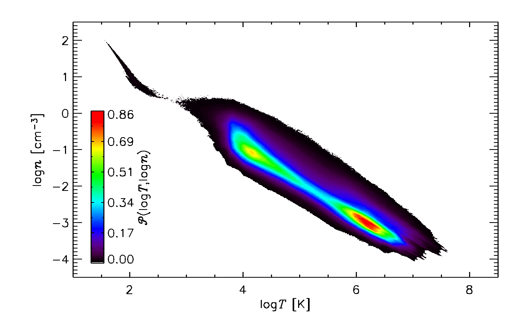
Figure 5.4: Total volume probability distributions of gas by temperature $T$ and density $n$. Eleven snapshots of Model WSWa in the interval $t=634$ to $644\,{\rm Myr}$ were used, with the system in a statistical steady state.

The probability distribution of gas number density and temperature is shown in Fig. 5.4 (model WSWa). While it is evident that there are large regions of pressure disequilibrium, there is clear evidence of three well defined phases, in which the pressure is perturbed about a line of constant thermal pressure, described by,

$$\log n=-\log T+{\rm constant}.$$

There are three distinct peaks at $(T[\,{\rm K}],n[\,{\rm cm^{-3}}])\simeq(10^{2},10)$, $(10^{4},10^{-1})$ and $(10^{6},10^{-3})$. The lines intersecting the maxima for the cold, warm and hot distributions at $(\log T,\log n)=(2,1.2),(4,-0.8),(6,-2.8)$, respectively, correspond to $p=k_{\rm B}nT=10^{-12.7}\,{\rm dyn}\,{\rm cm}^{-2}$. A reasonable identification of the boundaries between these phases is via the minima at about $500\,{\rm K}$ and $5\times 10^{5}\,{\rm K}$.

Having divided the gas along these boundaries, the probability distributions within each phase of gas number density $n$, turbulent r.m.s. velocity $u_{\rm turb}$, Mach number $\mathcal{M}$, thermal pressure $p$ and total pressure $P$ are displayed in Fig. 5.5, from Model WSWa.

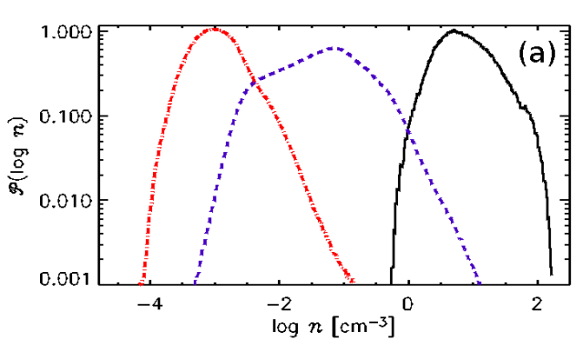
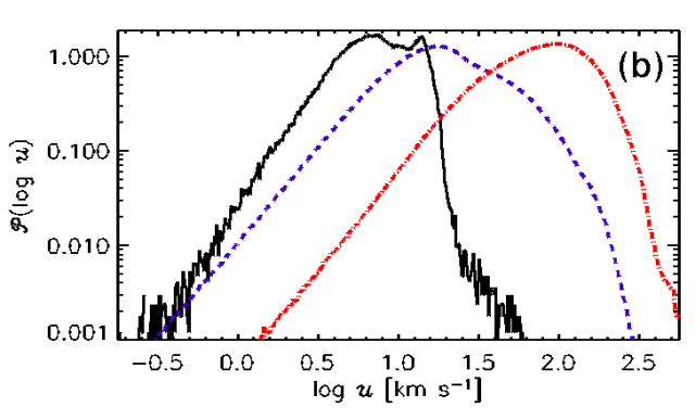
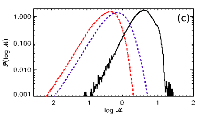
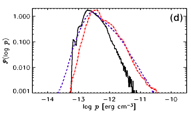
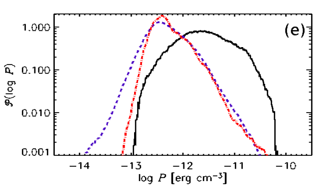
Figure 5.5: Total volume probability distribution of (a) density, (b) turbulent velocity, ${{\mbox{\boldmath$u$}}}_{\rm turb}$ (c) Mach number (defined with respect to the local speed of sound and ${{\mbox{\boldmath$u$}}}_{\rm turb}$), (d) thermal pressure, and (e) total pressure, for each phase of Model WSWa, using eleven snapshots spanning $t=634$ to $644\,{\rm Myr}$. The phases are: cold $T<500\,{\rm K}$ (black, solid line), warm $500\leq T<5\times 10^{5}\,{\rm K}$ (blue, dashed), and hot $T\geq 5\times 10^{5}\,{\rm K}$ (red, dash-dotted).

The overlap in the gas density distributions (Fig. 5.5a) is small. The modal densities that typify each of the hot, warm and cold gas are $10^{-3}$, $10^{-1}$ and $10\,{\rm cm^{-3}}$, respectively. Cold, dense clouds are formed through radiative cooling facilitated by compression; the latter, however, is truncated at the grid scale of 4 pc, preventing compression to the higher densities in excess of about $10^{2}\,{\rm cm^{-3}}$. From the comparison with the higher resolution Model WSWah in Fig. 5.3, it is evident that the separation into phases is more distinct with increased numerical resolution and that the anti-correlation between temperature and density is stronger. Hence the distinction between the density distributions evident in Fig. 5.5a, is even more pronounced when applied to high resolution.

The velocity probability distributions in Fig. 5.5b reveal a clear connection between the magnitude of the turbulent velocity of gas and its temperature: the r.m.s. velocity in each phase scales with its speed of sound. This is confirmed by the Mach number distributions in Fig. 5.5c: both warm and hot phases are transonic with respect to their sound speeds. The cold gas is mostly supersonic, having speeds typically under $10\,{\rm km\,s^{-1}}$. The double peak in velocity (Fig. 5.5b) is a robust feature, not dependent on the temperature boundary. This likely includes ballistic gas in SN remnants, as well as bulk transport by ambient gas at subsonic or transonic speed with respect to the warm gas.

Probability densities of thermal pressure, shown in Fig. 5.5d, are notable for their relatively narrow spread: one order of magnitude, compared to a spread of six orders of magnitude in gas density. Moreover, the three phases have overlapping distributions, suggesting that the system is in statistical thermal pressure balance. However, thermal pressure is not the only part of the total pressure in the gas. In the Galaxy, contributions to the pressure also arise from the turbulent pressure associated with the random motions and the cosmic ray and magnetic pressures. The turbulent pressure, $p_{\rm turb}=\frac{1}{3}\rho u^{2}_{\rm turb}$ is included in $P$ for Fig. 5.5e. The random motions $|{{\mbox{\boldmath$u$}}}_{\rm turb}|^{2}$ are derived by subtracting the mean flows ${\langle|{{\mbox{\boldmath$u$}}}|^{2}\rangle}_{\ell}$ from the total $|{{\mbox{\boldmath$u$}}}|^{2}$ (see Chapter 8 for explanation with respect to $B$). In Model WSWa the cosmic ray and magnetic pressures are absent.

The total pressure distribution for the hot gas differs little from the thermal pressure. The modal warm pressure increases only by about 25% at around $3\times 10^{-13}\,{\rm dyn}\,{\rm cm}^{-2}$. For the cold gas the modal pressure increases about ten fold from $2\times 10^{-13}\,{\rm dyn}\,{\rm cm}^{-2}$ to $2\times 10^{-12}\,{\rm dyn}\,{\rm cm}^{-2}$. The cold gas appears over pressured as a result. It becomes apparent (cf. below Fig. 5.7) that this is due to the vertical pressure gradient. All the cold gas occupies the higher pressure mid-plane, while the warm and hot gas distributions mainly include lower pressure regions away from the disc.

Theoretically, it might be expected that the densities of a gas subjected to multiple shocks may adopt a lognormal distribution rather than a normal distribution (Kevlahan and Pudritz, 2009). The probability distributions for density in Fig. 5.5a can be reasonably approximated by lognormal distributions, of the form

$$\mathcal{P}(n)=\Lambda(\mu_{n},s_{n})\equiv\frac{1}{ns_{n}\sqrt{2\upi}}\exp\left({\displaystyle-\frac{(\ln n-\mu_{n})^{2}}{2s_{n}^{2}}}\right).$$ (5.1)

The quality of the fits is good, but less so for the hot gas. This is improved when the hot gas is subdivided into that near the mid-plane ($|z|\leq 200\,{\rm pc}$) and that at greater heights ($|z|>200\,{\rm pc}$); the former dominated by very hot gas in the interior of SN remnants, the latter predominantly more diffuse gas in the halo. These fits are illustrated in Fig. 5.6, using 500 data bins in the range $10^{-4.8}<n<10^{2.5}\,{\rm cm}^{-3}$, where the warm gas has also been subdivided by height; the best-fit parameters are given in Table 5.1.

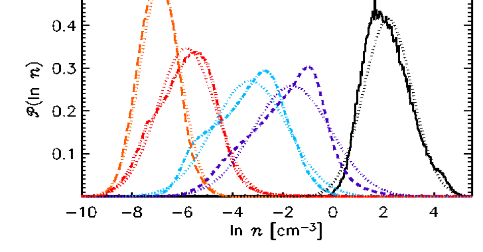
Figure 5.6: Density probability distributions for model WSWa, together with the best-fit lognormal distributions (dotted) for the cold (black, solid), warm and hot gas. The warm/hot gas have been divided into regions $|z|\leq 200\,{\rm pc}$ (blue/red, dashed/dash-3dotted) and $|z|>200\,{\rm pc}$ (light blue/orange, dash-dotted/long dashed) respectively.

The two types of hot gas have rather different density distributions, and separating them in this way significantly improves the quality of the lognormal fits. The warm gas distributions remain very similar, with identical variance but shifted to lower density above $|z|=200\,{\rm pc}$. It therefore appears justified to consider the two hot gas components separately, where it appears strongly affected by its proximity to the SN activity. The structure of the warm gas appears independent of the SN activity, and merely exhibits a dependence on the global density gradient, so it make sense to consider the warm gas as a single distribution. All distributions are fitted to lognormals at or above the 95% level of significance applying the Kolmogorov-Smirnov test. Although the warm gas density is well described by a lognormal distribution, there is the appearance of power law behaviour (Fig. 5.6) in its low density tail.

Probability distributions of the pressure, displayed in Fig. 5.7, show that although the thermal pressure of the cold gas near the mid-plane is out of equilibrium with the other phases the total pressures are all much closer to equilibrium. The gas at $|z|>200\,{\rm pc}$ (dotted lines) are in both thermal and total pressure balance. Thus by including the effect of the global pressure gradient, there is even stronger evidence to support the concept of pressure equilibrium between the phases.

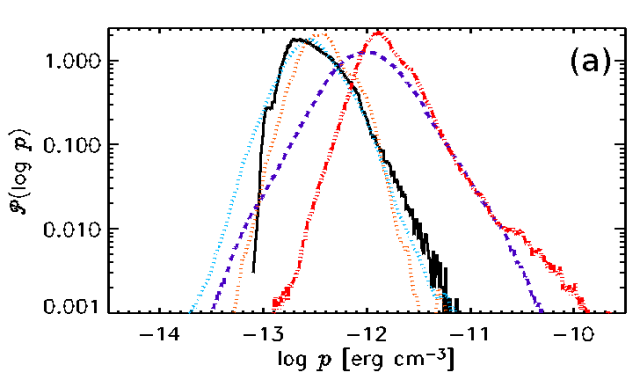
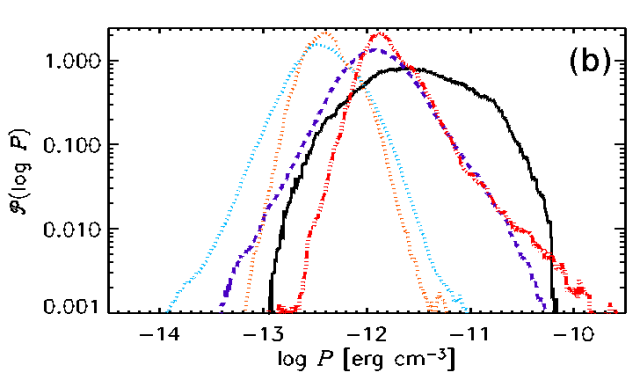
Figure 5.7: Probability distributions for (a) thermal pressure $p$ and (b) total pressure $P$ in Model WSWa, separately for the cold (black, solid), warm and hot gas. The warm/hot gas have been divided into regions $|z|\leq 200\,{\rm pc}$ (blue/red, dashed/dash-3dotted) and $|z|>200\,{\rm pc}$ (light blue/orange, dash-dotted/long dashed) respectively.

The broad lognormal distribution of $P$ for the cold gas is consistent with multiple rarefaction and compression due to shocks. The hot and warm gas pressure distributions however appear to follow a power law. Away from the mid-plane their pressure distributions have a similar shape, but slightly narrower. The density distribution for the hot gas is also narrower for $|z|>200\,{\rm pc}$, although not so the warm gas. This indicates that the gas away from the SN active mid-plane is, understandably, more homogeneous.

The time-averaged vertical density profiles obtained under the different numerical resolutions are shown in Fig. 5.8. Although the density distribution in Fig. 5.3a reveals higher density contrasts with increased resolution, there is little difference in the $z$-profiles of the models. The mean gas number density at the mid-plane $n(0)$, which with the coarse grid resolution excludes the contribution from Hii, is about $2.2\,{\rm cm^{-3}}$, double the observation estimates summarised in Ferrière (2001). This might be expected in the absence of the magnetic and cosmic ray components of the ISM pressure, to support the gas against the gravitational force.

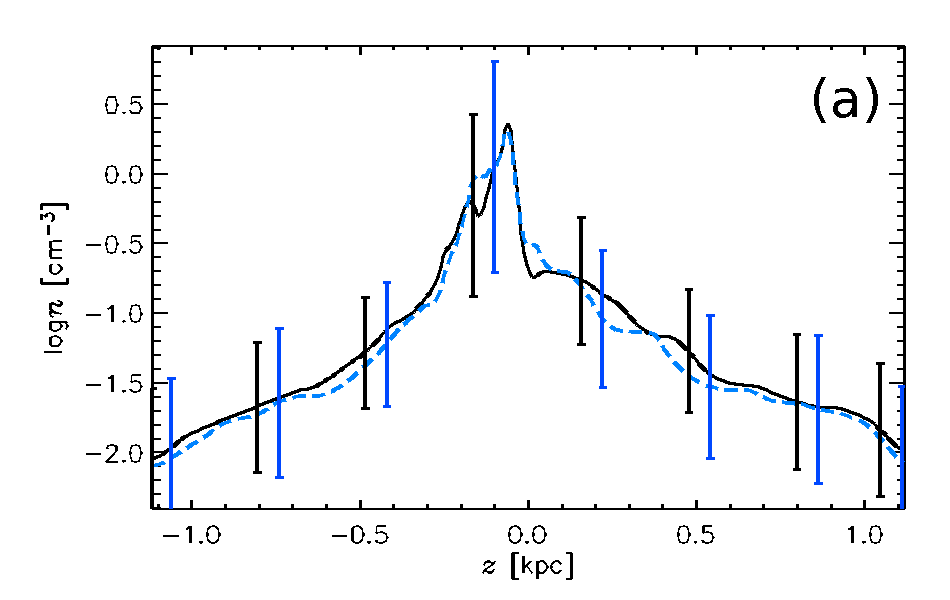
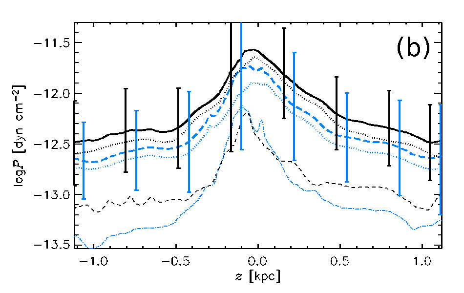
Figure 5.8: Horizontal averages of gas number density, $\overline{n}(z)$ (a), and total pressure, $\overline{P}(z)$ (b), for Model WSWa (solid, black), and Model WSWah (dashed, blue). Each are time-averaged using six and ten snapshots respectively, spanning 633 to 638 Myr. The vertical lines indicate standard deviation within each horizontal slice. The thermal $\overline{p}(z)$ (dotted) and ram $\overline{p}_{\rm turb}(z)$ (fine dashed) pressures are also plotted (b).

However the vertical pressure distributions are consistent with the models of Boulares and Cox (1990, their Fig. 1 and 2), which include the weight of the ISM up to $|z|=5\,{\rm kpc}$. The total pressure $P(0)\simeq 2.5~{}(2.0)\times 10^{-12}\,{\rm dyn}\,{\rm cm}^{-2}$ for the standard (high) resolution model is slightly above their estimate of about 1.9 for hot, turbulent gas. For the turbulent pressure alone $p_{\rm turb}(0)\simeq 6.3~{}(7.9)\times 10^{-13}\,{\rm dyn}\,{\rm cm}^{-2}$ falling to $1.0~{}(0.6)$ for $|z|=500\,{\rm pc}$ and then reasonably level. Together with the narrower pressure and density distributions for gas at $|z|>200\,{\rm pc}$, discussed above, this indicates that the pressure gradient above $500\,{\rm pc}$ is weak and this gas remains relatively homogeneous in comparison to gas near the mid-plane. The pressures are generally slightly reduced with increased resolution, except for $p_{\rm turb}$ near the mid-plane. Small scales are better resolved, so the turbulent structures are a stronger component of the SN active region. These pressures are consistent with Boulares and Cox (1990) even though our model does not explicitly include the pressure contributions from the ISM above $1\,{\rm kpc}$.

Comparing the thermal pressure distribution (Fig. 5.3c) with de Avillez and Breitschwerdt (2004, their Fig. 4a) and Joung, Mac Low and Bryan (2009, their Fig. 2) the peaks are at 3.16, 1.3 and $4.1\times 10^{-13}\,{\rm dyn}\,{\rm cm}^{-2}$, respectively. The model of de Avillez and Breitschwerdt (2004) include the gas up to $|z|=10\,{\rm kpc}$ and resolution up to 1.25 pc, and has the lowest modal pressure. Joung, Mac Low and Bryan (2009) model up to $|z|=10\,{\rm kpc}$, but include only gas within $125\,{\rm pc}$ of the mid-plane for the pressure distribution, and have the highest modal value. Data in Fig. 5.3c is for the total volume within $|z|=1\,{\rm kpc}$, having a modal pressure between the other two models.

It is reasonable to conclude that the main effects of the increased resolution are confined to the very hot interiors and to the thin shells of SN remnants; the interiors become hotter and the SN shell shocks become thinner with increased resolution (see Appendix A). Simultaneously, the higher density of the shocked gas enhances cooling, producing more cold gas and reducing the total thermal energy. Otherwise, the overall structure of the diffuse gas is little affected: the probability distributions of thermal pressure are almost indistinguishable, with the standard resolution having a fractionally higher pressure (Fig. 5.3c). We can conclude that the numerical resolution of the reference model, $\Delta=4\,{\rm pc}$, is sufficient to model the diffuse gas phases reliably. This choice of the working numerical resolution is further informed by tests described in Appendix A.

To summarise: the system is close to a state of statistical pressure equilibrium, with the total pressure having similar values and similar probability distributions in each phase. Joung, Mac Low and Bryan (2009) also conclude from their simulations that the gas is in both thermal and total pressure balance. This could be expected, since the only significant deviation in the statistical dynamic equilibrium of the system is the vertical outflow of the hot gas and entrained warm clouds (see Section 6.1).

5.2 The filling factor and fractional volume

5.2.1 Filling factors: basic concepts

The fractional volume of the ISM occupied by the phase $i$ is given by

$$f_{V,i}=\frac{V_{i}}{V}$$ (5.2)

where $V_{i}$ is the volume occupied by gas in the temperature range defining phase $i$ and $V$ is the total volume. How the gas is distributed within a particular phase is described by the phase filling factor

$$\phi_{i}=\frac{\overline{n_{i}}^{2}}{\overline{n_{i}^{2}}}\;,$$ (5.3)

where the over bar denotes a phase average, i.e., an average only taken over the volume occupied by the phase $i$. $\phi_{i}$ describes whether the gas density of a phase is homogeneous $\phi_{i}=1$ or clumpy $\phi_{i}<1$. Both of these quantities are clearly important parameters of the ISM, allowing one to characterise, as a function of position, both the relative distribution of the phases and their internal structure. As discussed below, the phase filling factor is also directly related to the idea of an ensemble average, an important concept in the theory of random functions and so $\phi_{i}$ provides a useful connection between turbulence theory and the astrophysics of the ISM. Both $f_{V,i}$ and $\phi_{i}$ are easy to calculate in a simulated ISM by simply counting mesh-points.

In the real ISM, however, neither $f_{V}$ nor $\phi_{i}$ can be directly measured. Instead the volume filling factor can be derived (Reynolds, 1977; Kulkarni and Heiles, 1988; Reynolds, 1991),

$${\Phi}_{i}=\frac{{\langle n_{i}\rangle}^{2}}{{\langle n_{i}^{2}\rangle}},$$ (5.4)

for a given phase $i$, where the angular brackets denote a volume average, i.e., taken over the total volume. Most observational work in this area to-date has concentrated on the diffuse ionized gas (or warm ionized medium) since the emission measure of the free electrons $\mathrm{EM}\propto n_{e}^{2}$ and the dispersion measure of pulsars $\mathrm{DM}\propto n_{e}$, allowing ${\Phi}$ to be estimated along many lines-of-sight (e.g. Reynolds, 1977; Kulkarni and Heiles, 1988; Reynolds, 1991; Berkhuijsen, Mitra and Mueller, 2006; Hill et al., 2008; Gaensler et al., 2008).

In terms of the volume $V_{i}$ occupied by phase $i$,

$$\overline{n_{i}}=\frac{1}{V_{i}}\int_{V_{i}}n_{i}\,dV,$$ (5.5)

whilst

$${\langle n_{i}\rangle}=\frac{1}{V}\int_{V}n_{i}\,dV=\frac{1}{V}\int_{V_{i}}n_{i}\,dV\,,$$ (5.6)

the final equality holding because $n_{i}=0$ outside the volume $V_{i}$ by definition. Since the two types of averages differ only in the volume over which they are averaged, they are related by the fractional volume:

$${\langle n_{i}\rangle}=\frac{V_{i}}{V}\overline{n_{i}}=f_{V,i}\overline{n_{i}},$$ (5.7)

and

$${\langle n_{i}^{2}\rangle}=\frac{V_{i}}{V}\overline{n_{i}^{2}}=f_{V,i}\overline{n_{i}^{2}}.$$ (5.8)

Consequently, the volume filling factor ${\Phi}_{n,i}$ and the phase filling factor $\phi_{n,i}$ are similarly related:

$${\Phi}_{i}=\frac{{\langle n_{i}\rangle}^{2}}{{\langle n_{i}^{2}\rangle}}=f_{V,i}\frac{\overline{n_{i}}^{2}}{\overline{n_{i}^{2}}}=f_{V,i}\phi_{i}.$$ (5.9)

Thus the parameters of most interest, $f_{V,i}$ and $\phi_{n,i}$, characterizing the fractional volume and the degree of homogeneity of a phase respectively, are related to the observable quantity ${\Phi}_{n,i}$ by Eq. (5.9). This relation is only straightforward when the ISM phase can be assumed to be homogeneous or if one has additional statistical knowledge, such as the probability density function, of the phase. In next sub-section we discuss some simple examples to illustrate how these ideas can be applied to the real ISM and also how the properties of our simulated ISM compare to earlier observations.

As with the density filling factors introduced above, filling factors of temperature and other variables can be defined similarly to Eqs. (5.3) and (5.4). Thus $\phi_{T,i}={\overline{T_{i}}^{2}}/{\overline{T_{i}^{2}}}$, etc.

5.2.2 Homogeneous-phase and lognormal approximations

To clarify the physical significance of the various quantities defined above, the relations between them are discussed in more detail. Consider Eqs. (5.2), (5.3) and (5.4) for an idealised two-phase system, where each phase is homogeneous. (The arguments can be generalised to an arbitrary number of homogeneous phases.) This scenario is often visualised in terms of discrete clouds of one phase, of constant density and temperature, being embedded within the other phase, of different (but also constant) density and temperature. The two phases might be, for example, cold clouds in the warm gas or hot regions coexisting with the warm phase. Let one phase have (constant) gas number density $N_{1}$ and occupy volume $V_{1}$, and the other $N_{2}$ and $V_{2}$, respectively. The total volume of the system is $V=V_{1}+V_{2}$.

The volume-averaged density of each phase, as required for Eq. (5.4), is given by

$${\langle n_{i}\rangle}=\frac{N_{i}V_{i}}{V}=f_{V,i}N_{i}.$$ (5.10)

where $i=1,2$. Similarly, the volume average of the squared density is

$${\langle n_{i}^{2}\rangle}=\frac{N_{i}^{2}V_{i}}{V}=f_{V,i}N_{i}^{2}.$$ (5.11)

The fractional volume of each phase can then be written as

$$f_{V,i}=\frac{{\langle n_{i}\rangle}^{2}}{{\langle n_{i}^{2}\rangle}}=\frac{{\langle n_{i}\rangle}}{N_{i}}={\Phi}_{n,i},$$ (5.12)

with $f_{V,1}+f_{V,2}=1$, and ${\Phi}_{n,1}+{\Phi}_{n,2}=1$. The volume-averaged quantities satisfy ${\langle n\rangle}={\langle n_{1}\rangle}+{\langle n_{2}\rangle}=f_{V,1}N_{1}+f_{V,2}N_{2}$ and ${\langle n^{2}\rangle}={\langle n_{1}^{2}\rangle}+{\langle n_{2}^{2}\rangle}=f_{V,1}N_{1}^{2}+f_{V,2}N_{2}^{2}$, with the density variance $\sigma^{2}\equiv{\langle n^{2}\rangle}-{\langle n\rangle}^{2}=f_{V,1}f_{V,2}(N_{1}-N_{2})^{2}$.

In contrast, the phase-averaged density of each phase, as required for Eq. (5.3), is simply $\overline{n_{i}}=N_{i}$, and the phase average of the squared density is $\overline{n_{i}^{2}}=N_{i}^{2}$, so that the phase filling factor is $\phi_{n,i}=1$. This ensures that Eq. (5.9) is consistent with Eq. (5.12). Thus, the phase filling factor is unity for each phase of a homogeneous-phase medium, and these filling factors clearly do not sum to unity in the case of multiple phases. This filling factor can therefore be used as a measure of the homogeneity of the phase (with a value of unity corresponding to homogeneity). On the contrary, the fractional volumes must always add up to unity, $\sum_{i}f_{V,i}=1$.

Thus for homogeneous phases, the volume filling factor and the fractional volume of each phase are identical to each other, ${\Phi}_{n,i}=f_{V,i}$, and both sum to unity when considering all phases; in contrast, the phase-averaged filling factor is unity for each phase, $\phi_{n,i}=1$. If a given phase occupies the whole volume (i.e., we have a single-phase medium), then all three quantities are simply unity: $\phi_{n,i}={\Phi}_{n,i}=f_{V,i}=1$.

Apart from the limitations arising from the inhomogeneity of the ISM phases, an unfortunate feature of the above definition of the volume filling factor (5.4), which hampers comparison with theory, is that the averaging involved is inconsistent with that used in the theory of random functions. In the latter, the calculation of volume (or time) averages is usually complicated or impossible and, instead, ensemble averages (over the relevant probability distribution functions) are used; the ergodicity of the random functions is relied upon to ensure that the two averages are identical to each other (Section 3.3 in Monin and Yaglom, 2007; Tennekes and Lumley, 1972). But the volume filling factors above are not compatible with such a comparison, as they are based on averaging over the total volume, despite the fact that each phase occupies only a fraction of it. In contrast, the phase averaging is performed only over the volume of each phase, and so should correspond better to results from the theory of random functions.

To illustrate this distinction, first note that, for the lognormal distribution, $\mathcal{P}(n_{i})\sim\Lambda(\mu_{n,i},s_{n,i})$, Eq. (5.1), the mean and mean-square densities are given by the following phase (‘ensemble’) averages:

$$\overline{n_{i}}=e^{\mu_{n,i}+s_{n,i}^{2}/2},~{}~{}\sigma_{i}^{2}=\overline{(n_{i}-\overline{n_{i}})^{2}}=\overline{n_{i}}^{2}\left(e^{s_{n,i}^{2}}-1\right),$$ (5.13)

where $\sigma_{i}^{2}$ is the density variance around the mean $\overline{n_{i}}$, so that

$$\phi_{n,i}=\frac{\overline{n_{i}}^{2}}{\overline{n_{i}^{2}}}=\frac{\overline{n_{i}}^{2}}{\sigma_{i}^{2}+\overline{n_{i}}^{2}}=\exp(-s_{n,i}^{2}).$$ (5.14)

With the filling factor thus defined, $\phi_{n,i}=1$ only for a homogeneous density distribution, $\sigma_{i}=0$ (or equivalently, $s_{n,i}=0$). This makes it clear that this filling factor, defined in terms of the phase average, is quite distinct from the fractional volume, but rather quantifies the degree of homogeneity of the gas distribution within a given phase. Both describe distinct characteristics of the multi-phase ISM, and, if properly interpreted, can yield rich information about the structure of the ISM.

5.2.3 Application to simulations

The definitions of filling factors and fractional volumes from Equations (5.2), (5.4) and (5.3) are applied to the phases identified in Section 5.1 for the HD reference model (WSWa). These are presented as horizontal averages in Fig. 5.9. Volumes are considered as discrete $4\,{\rm pc}$ thick slices spanning the full horizontal area. The cold, warm and hot phases are $T<5\times 10^{2}\,{\rm K}$, $5\times 10^{2}\,{\rm K}<T<5\times 10^{5}\,{\rm K}$ and $T>5\times 10^{5}\,{\rm K}$, respectively.

Figure 5.9: Horizontal averages for cold (black, solid line), warm (blue, dashed) and hot (red, dash-dotted) of the gas density (a) phase-averaged filling factors $\phi_{n}$, (b) volume-averaged filling factors ${\Phi}_{n}$ and (c) fractional volumes $f_{V}$. Results plotted are from 21 snapshots in the interval $636$ to $646\,{\rm Myr}$ for Model WSWa.

The hot gas (Fig. 5.9c) accounts for about 60% of the volume at $|z|\simeq 1\,{\rm kpc}$ and about 50% near the mid-plane. The local maximum of the fractional volume of the hot gas at $|z|\,\hbox to0.0pt{\raise 2.15277pt\hbox{$<$}\hss}{\lower 4.30554pt\hbox{$\sim$}}\,200\,{\rm pc}$ is due to the highest concentration of SN remnants there. A conspicuous contribution to various diagnostics – especially within $200\,{\rm pc}$ of the mid-plane, where most of the SNe are localised – comes from the very hot gas within SN remnants. Regarding its contribution to integrated gas parameters, it should perhaps be considered as a separate phase.

Now how robust are results based on the assumption that each phase is homogeneous? How strongly does the inhomogeneity of the ISM phases affect the results? Note immediately that, unlike the fractional volumes, the filling factors do not add up to unity, $\sum_{i}{\Phi}_{n,i}\neq 1$, if any phase $i$ is not homogeneous. Figure 5.9b displays the vertical profiles of the density filling factors ${\Phi}_{n,i}={\langle n_{i}\rangle}^{2}/{\langle n_{i}^{2}\rangle}$ computed for each phase in the reference model, as in Eq. (5.4). (As these are functions of $z$, the averaging here is in two dimensions, over horizontal planes; the distinction between the total plane and that part of the plane occupied by the relevant phase remains relevant, however.) This should be compared with the fractional volumes shown in Fig. 5.9c. For all three phases, the values of ${\Phi}_{n,i}$ are smaller than $f_{V,i}$ and the peak near the mid-plane evident for the hot gas in $f_{V,i}$ is absent in ${\Phi}_{n,i}$. The volume density filling factors in Fig. 5.9a are closest to unity for the cold gas (near the mid-plane, where such gas is abundant), indicating that this phase is more homogeneous than the other phases.

Table 5.1: Statistical parameters of the distribution of gas number density $n$ in various phases for Model WSWa, and their lognormal and homogeneous-phase approximations. Figures in Part (A) have been calculated directly from a composite of 11 simulation snapshots, those in (B) and (C) represent the best-fit lognormal and homogeneous-phase approximations to the data in (A), respectively: $\mu_{n}$ and $s_{n}$ are defined in Eq. (5.1); $\overline{n}$ and $\sigma$ are the mean and standard deviation of $n$; $\phi_{n}$, $f_{V}$ and ${\Phi}_{n}$ are the phase filling factor, the fractional volume and the volume filling factor, respectively, as defined in Section 5.2.1. The lower (${\rm Q}_{1}$) and upper (${\rm Q}_{3}$) quartiles and the median of the density distributions are given in the last three columns. Standard deviation for each mean between the simulation snapshots as % of $\overline{n}$ is shown in brackets.

Phase	$\mu_{n}$	$s_{n}$	$\overline{n}$	$\sigma$	$\phi_{n}$	$f_{V}$	${\Phi}_{n}$	$\displaystyle\frac{\phi_{n}f_{V}}{{\Phi}_{n}}$	${\rm{Q}}_{1}$	Median	${\rm{Q}}_{3}$
	$[\ln\,{\rm cm^{-3}}]$	$[\ln\,{\rm cm^{-3}}]$	$[\!\,{\rm cm^{-3}}]$	$[\!\,{\rm cm^{-3}}]$					$[\!\,{\rm cm^{-3}}]$	$[\!\,{\rm cm^{-3}}]$	$[\!\,{\rm cm^{-3}}]$
(A) Gas density from the simulation
Cold			$12.6\quad~{}(9\%)$	$15.90$	$0.384$	$0.004$	$0.0016$	$1.000$	$3.9$	$7.1$	$14.2$
Warm			$0.14\quad~{}(3\%)$	$0.48$	$0.080$	$0.608$	$0.0486$	$0.999$	$0.019$	$0.049$	$0.16$
Hot ($|z|\leq 200\,{\rm pc}$)			$0.0062~{}(13\%)$	$0.019$	$0.124$	$0.057$	$0.0039$	$0.178$	$0.0013$	$0.0032$	$0.0066$
Hot ($|z|>200\,{\rm pc}$)			$0.0013~{}(10\%)$	$0.0016$	$0.457$	$0.331$	$0.1850$	$0.819$	$0.00057$	$0.00097$	$0.0017$
(B) The lognormal approximation (5.1) to the gas density probability distribution in each phase
Cold	$\phantom{-}2.02$	$0.92$	$11.5$	$13.3$	$0.43$	$0.004$	$0.0016^{*}$	$1$	$4.1$	$7.5$	$13.9$
Warm	$-3.03$	$1.47$	$0.14$	$0.39$	$0.115$	$0.422$	$0.0486^{*}$	$1$	$0.017$	$0.048$	$0.14$
Hot ($|z|\leq 200\,{\rm pc}$)	$-5.78$	$1.20$	$0.0063$	$0.011$	$0.24$	$0.003$	$0.0039^{*}$	$0.179$	$0.0014$	$0.0031$	$0.0069$
Hot ($|z|>200\,{\rm pc}$)	$-6.96$	$0.77$	$0.0013$	$0.0011$	$0.55$	$0.276$	$0.1850^{*}$	$0.821$	$0.00056$	$0.00094$	$0.0016$
(C) The homogeneous phase approximation
Cold			$12.6$	$0$	$1$	$0.002$	$0.0016^{*}$	$1$	$12.6$	$12.6$	$12.6$
Warm			$0.14$	$0$	$1$	$0.049$	$0.0486^{*}$	$1$	$0.14$	$0.14$	$0.14$
Hot ($|z|\leq 200\,{\rm pc}$)			$0.0062$	$0$	$1$	$0.007$	$0.0039^{*}$	$0.179$	$0.0062$	$0.0062$	$0.0062$
Hot ($|z|>200\,{\rm pc}$)			$0.0013$	$0$	$1$	$0.152$	$0.1850^{*}$	$0.821$	$0.0013$	$0.0013$	$0.0013$
∗ indicates a fixed value, taken from part (A)

Table 5.1 illustrates the meaning and significance of the quantities introduced above. The first part, (A), presents results for the actual density distribution from Model WSWa. The volume filling factors $\Phi_{n}$ for the hot gas have been adjusted for the whole volume, since they are calculated over only 0.2 and 0.8 of the total volume, respectively. Thus, the hot gas at $|z|\leq 0.2\,{\rm kpc}$ ($|z|>0.2\,{\rm kpc}$) occupies $0.275$ ($0.410$) of that volume, but $0.055$ ($0.331$) of the total volume.

Part (A) of the table allows confirmation, by direct calculation of the the quantities involved, that Eq. (5.9) is satisfied to high accuracy, i.e., $\phi_{n}f_{V}/{\Phi}_{n}=1$ for each phase. Because the statistical parameters involved are averaged over time, this relation is not exact, but is satisfied exactly for each snapshot. Similarly, $\phi_{n}=\overline{n}^{2}(\sigma^{2}+\overline{n}^{2})$ only approximately, whereas the equality is satisfied very accurately for each snapshot.

Part (B) of the table provides the parameters, $\mu_{n}$ and $s_{n}$, of the best-fit lognormal approximations to the probability distributions of the gas density shown in Fig. 5.6. Using Eq. (5.13), $\overline{n}$ and $\sigma$ are derived and then Eq. (5.14) is used to determine each $\phi_{n}$. $f_{V}$ is taken directly from the simulation data, i.e. from Part (A), and Eq. (5.9) is used to calculate ${\Phi}_{n}$.

The accuracy of the lognormal approximation to the density PDFs is characterized by the values of the mean density $\overline{n}$, its standard deviation $\sigma$ and the two filling factors, as compared to the corresponding quantities in (A). The approximation is quite accurate for the mean density and $\sigma$. The median (Q₂) and the lower and upper quartiles (Q₁ and Q₃) of the density distribution, are derived

$${\rm Q}_{2}=e^{\mu_{n}},\quad{\rm Q}_{1,3}=e^{\mu_{n}\pm 0.67s_{n}}$$

and shown in the last three columns, are also reasonably consistent between Parts (A) and (B). The most significant disparity is apparent in the cold gas, where the skew in the real distribution is stronger than evident in the lognormal approximation. Even here the differences are modest, and for the warm and hot gas the agreement is excellent.

Finally, Part (C) allows one to assess the consequences of an assumption of homogeneous-phases, where $\phi_{n}=1$ and $f_{V}={\Phi}_{n}$ for each phase by definition. The values of ${\Phi}_{n}$ obtained under this approximation are very significantly in error (by a factor 3–10). The last two columns of the table suggest the reason for that: perhaps unexpectedly, this approximation is strongly biased towards higher densities for all phases, except for the cold gas (which occupies negligible volume), so that the gas density within each phase obtained with this approximation is very close to the upper quartile of the probability distribution and thus misses significant amounts of a relatively rarefied gas in each phase.

In conclusion the lognormal approximation to the gas density distribution provides much more accurate estimates of the fractional volume than the homogeneous-phase approximation, at least for the model ISM. This should be borne in mind when observational data are interpreted in terms of filling factors.

Comparing the gas density distribution shown in Fig. 5.3a with the higher resolution run Model WSWah, the mean warm gas density ($0.14\,{\rm cm}^{-3}$) and the minimum in the distribution ($10^{-2}\,{\rm cm}^{-3}$) appears to be independent of the resolution. However the natural log mean $\mu_{n}\simeq-8$ for the hot gas within and without $200\,{\rm pc}$ of the mid-plane, but with larger standard deviation for the gas near the mid-plane. This compares with -6.96 and -5.78 in Table 5.1 for $4\,{\rm pc}$ resolution, i.e. about 1/3. This reflects the improved resolution of low density in the remnant interior.

5.2.4 Observational implications

Here I consider how these results might be used to interpret observational results. Observations can be used to estimate the volume-averaged filling factor ${\Phi}_{n,i}$, defined in Eq. (5.4), for a given ISM phase. On its own, this quantity is of limited value in understanding how the phases of the ISM are distributed: of more use are the fractional volume occupied by the phase $f_{V,i}$, defined in Eq. (5.2), and its degree of homogeneity which is quantified by $\phi_{n,i}$, defined by Eq. (5.3). Knowing ${\Phi}_{n,i}$ and $\phi_{n,i}$, $f_{V,i}$ follows via Eq. (5.9):

$$f_{V,i}=\frac{{\Phi}_{n,i}}{\phi_{n,i}}.$$ (5.15)

This formula is exact, but its applicability in practise is limited if $\phi_{n,i}$ is unknown. However $\phi_{n,i}$ can be deduced from the probability distribution of $n_{i}$: for example if the density probability distribution of the phase can be approximated by the lognormal, then $\phi_{n,i}$ can be estimated from Eq. (5.14).

Berkhuijsen, Mitra and Mueller (2006) and Berkhuijsen and Müller (2008) estimated ${\Phi}_{n,\rm DIG}$ for the diffuse ionized gas (DIG) in the Milky Way using dispersion measures of pulsars and emission measure maps. In particular, Berkhuijsen, Mitra and Mueller (2006) obtain ${\Phi}_{n,\rm DIG}\simeq 0.24$ towards $|z|=1\,{\rm kpc}$, and Berkhuijsen and Müller (2008) find the smaller value ${\Phi}_{n,\rm DIG}\simeq 0.08$ for a selection of pulsars that are closer to the Sun than the sample of Berkhuijsen, Mitra and Mueller (2006). On the other hand, Berkhuijsen and Fletcher (2008) and Berkhuijsen and Fletcher (2012) used similar data for pulsars with known distances to derive PDFs of the distribution of DIG volume densities which are well described by a lognormal distribution; the fitted lognormals have $s_{\rm DIG}\simeq 0.22$ at $|b|>5\deg$ (Table 1 in Berkhuijsen and Fletcher, 2012). Using Eqs. (5.14) and (5.15), this implies that the fractional volume of DIG, with allowance for its inhomogeneity, is about

$$f_{V,\rm DIG}\simeq 0.1\mbox{--}0.2.$$

In other words these results imply that the DIG is approximately homogeneous. Berkhuijsen and Fletcher (2008) also fitted lognormal distributions to the volume densities of the warm Hi along lines-of-sight to 140 stars (although no filling factors could be calculated for this gas): they found $s_{\mathrm{HI}}\simeq 0.3$, again suggesting that this phase of the ISM is approximately homogeneous. Corrections for the inhomogeneity in the fractional volume only become significant when $s_{i}\,\hbox to0.0pt{\raise 2.15277pt\hbox{$>$}\hss}{\lower 4.30554pt\hbox{$\sim$}}\,0.5$; by a factor of 1.3 for $s_{i}=0.5$ and a factor of 2 for $s_{i}=0.8$.

5.3 Three-phase structure defined using specific entropy

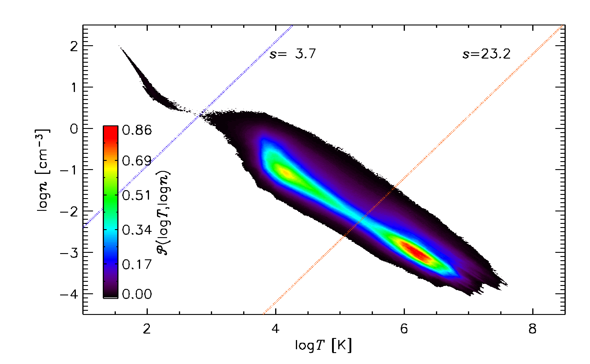
Figure 5.10: PDF contour plot by volume of log$n$ vs log$T$ for Model S${\Omega}$, averaged over 200 Myr. The lines of constant specific entropy $s=3.7\cdot 10^{8}$ and $23.2\cdot 10^{8}\,{\rm erg}\,{\rm g}^{-1}\,{\rm K}^{-1}$ indicate where the phases are defined as cold for $s\leq 3.7$ and as hot for $s>23.2$.

In Section 5.1 the three phase medium was defined according to temperature bands. This definition unfortunately precludes any statistically meaningful description of the temperature distribution of each phase, as these are effectively just the total temperature distribution split into three disjoint segments. It is evident that there is likely to be some overlap in the distribution of temperatures between the phases; considering the similarities between the cold phase and colder gas in the warm phase, and between the hot phase and the hotter gas in the warm phase, as described in Section 5.4.

With reference to Fig. 5.4, where the probability distribution of $T,n$ is displayed as 2D contours, the gas is spread across regions out of pressure equilibrium about a line of constant thermal pressure, corresponding to $p\simeq k_{\rm B}nT=10^{-12.7}\,{\rm dyn}\,{\rm cm}^{-2}$. This is reproduced in Fig. 5.10. The minima of the probability distribution may be considered to be aligned roughly perpendicular to the line of constant pressure, intersecting at $\log T\simeq 2.75\,{\rm K}$ and $\log T\simeq 5.25\,{\rm K}$.

Specific entropy is related to temperature and density by

$$s={\,{c_{\rm v}}}\left[\ln T-\ln T_{0}-(\gamma-1)(\ln\rho-\ln\rho_{0})\right],$$

with $\,{c_{\rm v}}$ denoting the specific heat capacity of the gas at constant volume and $\gamma=5/3$ the adiabatic index. Note that $s=0$ when both $T=T_{0}$ and $\rho=\rho_{0}$. Lines of constant specific entropy in Fig. 5.10 take the form $\log n-1.5\log T=$ constant. The dotted lines plotted identify the cold phase as occurring where $s<3.7\cdot 10^{8}\,{\rm erg}\,{\rm g}^{-1}\,{\rm K}^{-1}$ (blue) and hot occurring where $s>23.2\cdot 10^{8}\,{\rm erg}\,{\rm g}^{-1}\,{\rm K}^{-1}$ (orange). Although these are not necessarily observable quantities, they can be calculated directly for the simulated data, and the various probability distributions determined, including the temperatures.

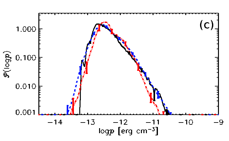
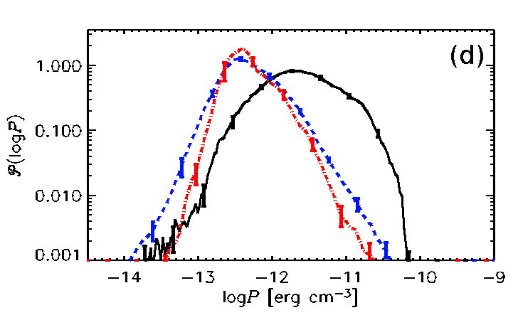
Figure 5.11: Distributions of entropy defined phases for Model WSWa: cold (black, solid), warm (blue, dashed) and hot (red, dash-dotted) for $\rho$, $T$, $p$, and $P$ (Panels a – d, respectively). Eleven snapshots are used spanning $t=634$ to $644\,{\rm Myr}$. Error bars indicate the 95% confidence interval accounting for deviations over time. The cold phase is defined to exist where specific entropy $s<3.7\cdot 10^{8}\,{\rm erg}\,{\rm g}^{-1}\,{\rm K}^{-1}$, hot where $s>23.2\cdot 10^{8}\,{\rm erg}\,{\rm g}^{-1}\,{\rm K}^{-1}$ and the warm phase in between.

In Fig. 5.11 the probability distributions for each phase defined by specific entropy from Model WSWa are displayed for $\rho$, $T$, $p$ and $P$ in panels (a – d) respectively, where $p$ is thermal pressure and $P$ is total pressure, as described in Section 5.1, so that it excludes cosmic ray and magnetic pressures, but include turbulent pressure.

The distribution of $n$ for the hot gas is slightly narrower, but the modal density remains $10^{-3}\,{\rm cm^{-3}}$. The warm gas distribution is however bi-modal with peaks at and more disjoint. The peaks in the distributions are consistent with the definitions in Section 5.1 at $10^{-3},10^{-1}$ and $10\,{\rm cm^{-3}}$ for hot, warm and cold respectively.

From panels (c) and (d) we can see that the peaks of the distributions are consistent with the line of constant pressure at $p=10^{-12.7}\,{\rm erg}\,{\rm cm^{-3}}$ referred to in Fig. 5.10. There is little change in the distributions of $p$, compared to Fig. 5.5. The differences in $P$ between the cold gas and the rest can be accounted for by the vertical pressure gradient as explained with reference to Fig. 5.7.

With this approach we can obtain credible probability distributions for temperature $T$ shown in panel (b). These distributions may help to qualify the characteristics of a region of the ISM from measurements of temperature, as the means and variances can be well defined for each phase and the regions of intersection are small.

5.4 Further results

In this section the distribution of the gas is explored more closely. The temperature of the ISM is more finely identified with a set of narrower bands as detailed in Table 5.2. As with the phases in Eq. (5.2) the fractional volume of each temperature range $i$ at a height $z$ can be given by

$$f_{V,i}(z)=\frac{V_{i}(z)}{V(z)}=\frac{N_{i}(z)}{N(z)},$$ (5.16)

where $N_{i}(z)$ is the number of grid points in the temperature range $T_{i,\mathrm{min}}\leq T<T_{i,\mathrm{max}}$, with $T_{i,\mathrm{min}}$ and $T_{i,\mathrm{max}}$ given in Table 5.2, and $N(z)$ is the total number of grid points at that height. The fractional mass is similarly calculated as

$$f_{M,i}(z)=\frac{M_{i}(z)}{M(z)},$$ (5.17)

where $M_{i}(z)$ is the mass of gas within temperature range $i$ at a given $z$, and $M(z)$ is the total gas mass at that height.

Table 5.2: Key to Figs. 5.12 and 7.5, defining the gas temperature bands used there.

Temperature band	Line style	Phase
$5\times 10^{1}\,{\rm K}<$$T<5\times 10^{1}\,{\rm K}$		cold
$5\times 10^{1}\,{\rm K}\leq T<5\times 10^{2}\,{\rm K}$	$\cdot$-$\cdot$-$\cdot$-$\cdot$-$\cdot$	cold
$5\times 10^{2}\,{\rm K}\leq T<5\times 10^{3}\,{\rm K}$	- - - - -	warm
$5\times 10^{3}\,{\rm K}\leq T<5\times 10^{4}\,{\rm K}$	– – – -	warm
$5\times 10^{4}\,{\rm K}\leq T<5\times 10^{5}\,{\rm K}$	–- $\cdot$- $\cdot$- –	warm
$5\times 10^{5}\,{\rm K}\leq T<5\times 10^{6}\,{\rm K}$	–$\cdots$–$\cdot$	hot
$5\times 10^{1}\,{\rm K}<$$T\geq 5\times 10^{6}\,{\rm K}$	$\cdots\cdots$	hot

Figure 5.12: Vertical profiles of (a) the fractional volume (Eq. 5.16) and (b) the fractional mass (Eq. 5.17) for Model WSWa, calculated for the temperature ranges given, along with the figure legend, in Table 5.2. Data from 21 snapshots were used spanning $636$ to $646\,{\rm Myr}$. Fractional volume (c) for Model WSWa and (d) for Model WSWah. Direct comparison from 6 (10) snapshots for Model WSWa (WSWah) in the reduced interval $633$ to $638\,{\rm Myr}$.

Note that the relative abundances of the various phases in these models might be affected by the unrealistically high thermal conductivity adopted. The coldest gas (black, solid), with $T<50\,{\rm K}$, is largely confined within about $200\,{\rm pc}$ of the mid-plane. Its fractional volume (Fig. 5.12a) is small even at the mid-plane, but it provides more than half of the gas mass at $z=0$ (Fig. 5.12b). Gas in the next temperature range, $50<T<500\,{\rm K}$ (purple, dash-dotted), is similarly distributed in $z$. Models WSWa and WSWah differ only in their resolution, using 2 and 4 pc, respectively. Model WSWah is a continuation of the state of WSWa after 600 Myr of evolution. With higher resolution the volume fraction of the coldest gas is significantly enhanced (Fig. 5.12d compared to b), but it is similarly distributed.

Gas in the range $5\times 10^{2}<T<5\times 10^{3}\,{\rm K}$ (dark blue, dashed) has a similar profile to the cold gas for both the fractional mass and the fractional volume, and this is insensitive to the model resolution. This is identified with the warm phase, but exists in the thermally unstable temperature range. It accounts for about 10% by volume and 20% by mass of the gas near the mid-plane. Heiles and Troland (2003) estimate at least 48% of the WNM to be in the thermally unstable range $500\,{\rm K}<T<5000\,{\rm K}$, and that the WNM accounts for 50% of the volume filling fraction at $|z|=0$. From Fig. 5.12a, assuming the WMN corresponds to the two bands within $500\,{\rm K}<T<50\,000\,{\rm K}$, in the model this account for roughly 50% of the total volume fraction for $|z|<400\,{\rm pc}$, and about 40% at $|z|\simeq 0$, with only a third of this in the unstable range. So the WMN is consistent with observation, although the model may slightly under represent the thermally unstable abundance. It is negligible away from the supernova active regions.

The two bands with $T>5\times 10^{5}\,{\rm K}$ (red, dotted and orange, dash-3dotted) behave similarly to each other, occupying similar fractional volumes for $|z|\,\hbox to0.0pt{\raise 2.15277pt\hbox{$<$}\hss}{\lower 4.30554pt\hbox{$\sim$}}\,0.75\,{\rm kpc}$, and with $f_{V,i}$ increasing above this height (more rapidly for the hotter gas). In contrast the fractional masses in these temperature bands are negligible for $|z|\,\hbox to0.0pt{\raise 2.15277pt\hbox{$<$}\hss}{\lower 4.30554pt\hbox{$\sim$}}\,0.75\,{\rm kpc}$, and increase above this height (less rapidly for the hotter gas). The temperature band $5\times 10^{4}<T<5\times 10^{5}\,{\rm K}$ (green/black, dash-3dotted) is identified with the warm phase, based on the minimum in the combined density and temperature distribution at $T\simeq 5\times 10^{5}\,{\rm K}$ in Fig. 5.4. However as a function of $z$ it is similarly distributed to the hotter gas (orange) in all profiles. This indicates it is likely a transitional range of mainly hot gas cooling, which accounts for a relatively small mass fraction of the warm gas. The dramatic effect of increased resolution (Fig. 5.12d compared to c) is the significant increase in the very hot gas (red, dotted), particularly displacing the hotter gases (orange and green) but also to some degree the warm gas (blue, dashed). This reflects the reduced cooling due to the better density contrasts resolved, associating the hottest temperatures to the most diffuse gas.

The middle temperature range $5\times 10^{3}<T<5\times 10^{4}\,{\rm K}$ has a distinctive profile in both fractional volume and fractional mass, with minima near the mid-plane and maxima at about $|z|\simeq 400\,{\rm pc}$, being replaced as the dominant component by hotter gas above this height. The fractional volume and vertical distribution of this gas is quite insensitive to the resolution.

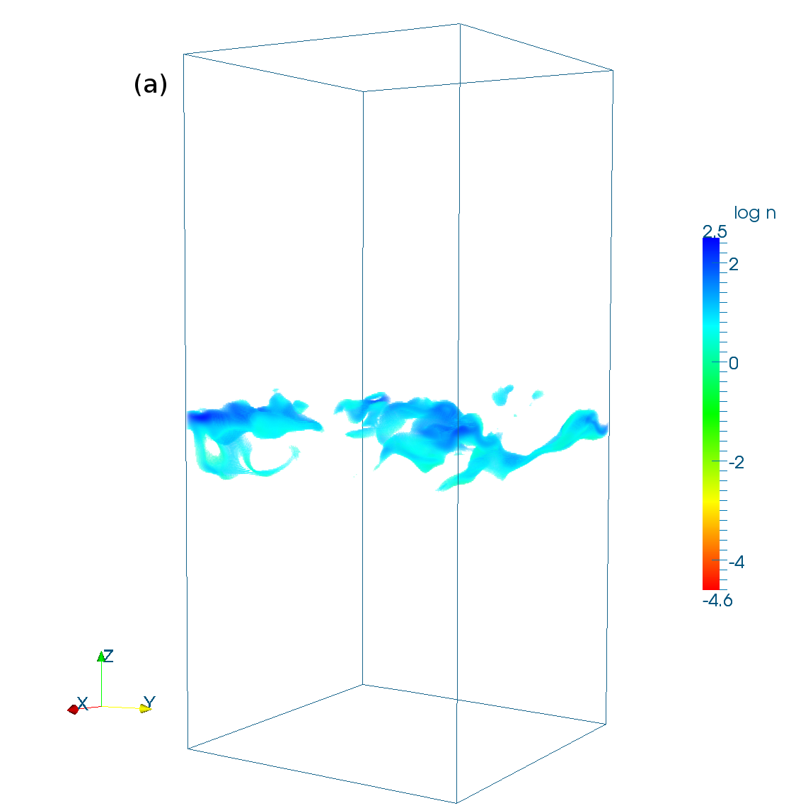
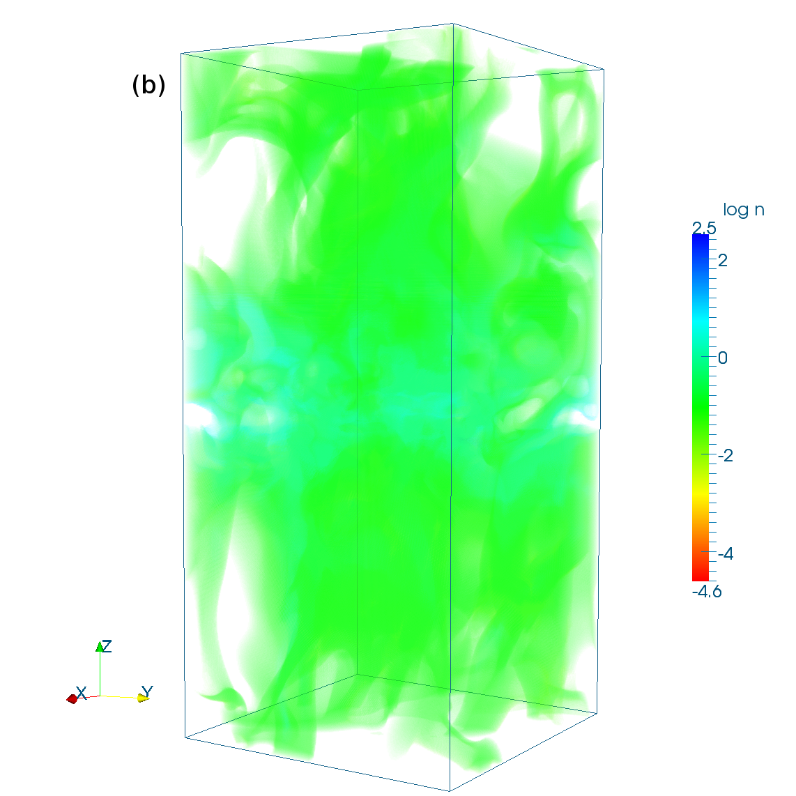
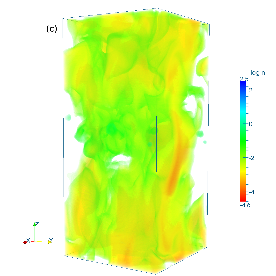
Figure 5.13: 3D snapshots, from Model WSWa, of gas number density in (a) the cold gas, (b) the warm gas, and (c) the hot gas. In each plot regions that are clear (white space) contain gas belonging to another phase. The phases are separated at temperatures $500\,{\rm K}$ and $5\times 10^{5}\,{\rm K}$. The colour scale for log $n$ is common to all three plots.

A three dimensional rendering of a snapshot of the density distribution from the reference model (WSWa) is illustrated in Fig. 5.13, showing the typical location and density composition of each phase separately. In panel a the cold gas is located near the mid-plane, apparently in layers with some more isolated fragments. The location and filling fraction of the warm (panel b) and hot (panel c) gas appear similar, although the hot gas has density typically 1/100 that of the warm gas density. The density of the gas is more roughly correlated with $z$, with the stongest fluctuations in the structure of the hot gas, including very diffuse regions scattered about the mid-plane as well as near the vertical boundaries.

The analysis of the warm gas density distribution within and outside the supernova active mid-plane in Section 5.1 indicated that its shape and standard deviation is fairly robust, and is merely shifted with respect to mean density, a predictable consequence of balancing the global pressure gradient. On the other hand the gas density distributions of the hot gas have been found to be quite different within and outside the mid-plane. In particular the distribution of hot gas near the mid-plane has a larger standard deviation, as well as increased mean. This is reflected in the pockets of very diffuse gas near the mid-plane, amongst the most dense hot gas.

The significance of these features to observations, are that the effects of the warm gas are more predictable, with consistent standard deviation, independent of height and in principle a predictable trend in the mean with respect to the pressure balance to the gravitational potential. For the hot gas observations along a line-of-sight above the supernova active region $|z|\simeq 300\,{\rm pc}$ will also have consistent standard deviation and trend in the mean. The structure of the hot gas near the mid-plane is significantly more complex and subject to strong local effects.

5.5 Summary

The ISM is reasonably described by separation into phases. The boundaries between the phases can be identified by the minima in the volume weighted probability distributions of the gas temperature. An alternative representation in terms of specific entropy for the phase boundaries also yields statistically meaningful phase temperature PDFs. The phases are well described by statistical thermal and total pressure balance. The phase PDFs for the gas density are lognormal, and applying these fits provides a better determination of the fractional volume from the phase filling factor than the assumption of homogeneous phases.

Chapter 6 Structure of the velocity field

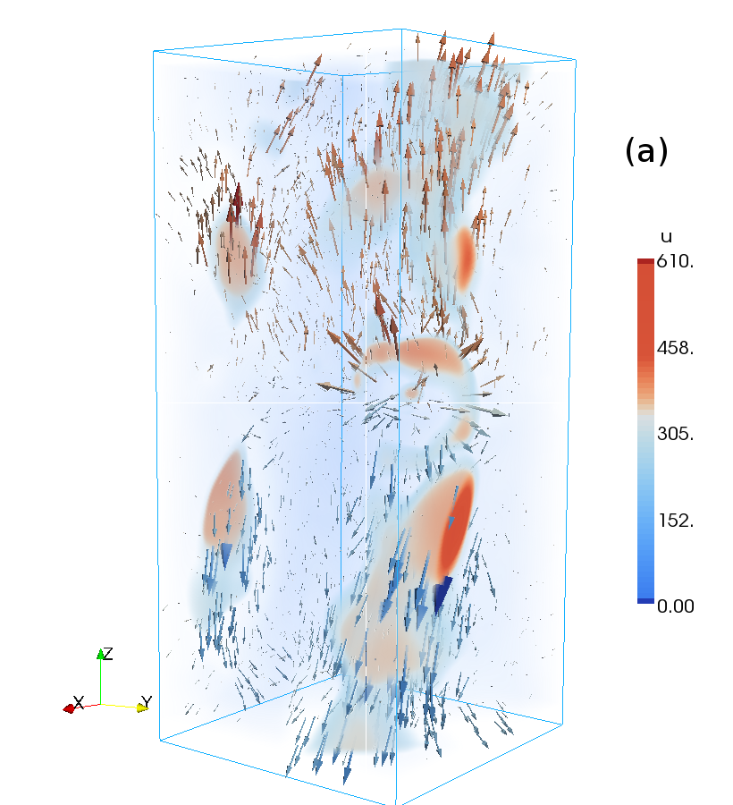
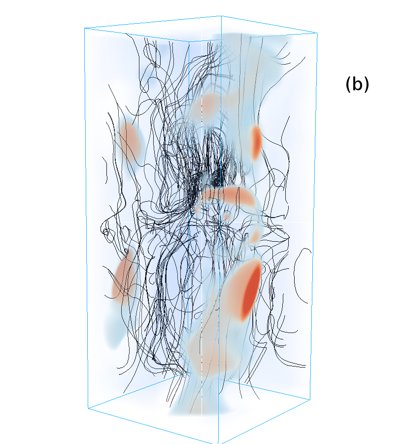
Figure 6.1: The perturbation velocity field $u$ in Model WSWa at $t=550\,{\rm Myr}$. The colour bar indicates the magnitude of the velocity depicted in the volume shading, with rapidly moving regions highlighted with shades of red. The low velocity regions, shaded blue, also have reduced opacity to assist visualisation. Arrow length of vectors (a) is proportional to the magnitude of $u$, with red (blue) arrows corresponding to $u_{z}>0$ ($u_{z}<0$) and independent of the colour bar. Trajectories of fluid elements (b) are also shown, indicating the complexity of the flow and its pronounced vortical structure.

Understanding the nature of the flows in the ISM is important for appreciating many other inter-related properties of the ISM. What are the systematic vertical flows? Can they be characterized as a wind sufficient to escape the gravitational potential of the galaxy and hence deplete the gas content or are they characteristic of a galactic fountain, in which case the gas is recycled? How does the velocity correlate with the density and hence contribute to kinetic energy and the energy balance in the galaxy, against thermal, magnetic and cosmic ray contributions? How is the velocity field divided between a mean flow and fluctuations? To what extent do these properties vary by phase? Over what scales are the turbulent eddies of the ISM correlated, and how do they depend on phase or vary as a function of height? What is the vortical structure of the ISM and what contributions do various features of the velocity field bring to the magnetic dynamo? In this section some of the general features of the velocity field are described and some characteristics of the flow by phase are considered. The correlation scales as a function of height are measured for the total ISM.

In Fig. 6.1 aspects of the velocity field in 3D for the reference Model WSWa are displayed. The volume rendering shows the regions of high speed. Speeds below about $300\,{\rm km\,s^{-1}}$ are transparent to aid visualisation. Velocity vectors are illustrated (panel a) using arrows, size indicating speed and colour the $z$-component. These indicate that flows away from the mid-plane are dominant. Red patches are indicative of recent SNe and there is a strongly divergent flow close to middle on the $xz$-face. In addition stream lines (b) display the presence of many small scale vortical flows near the mid-plane.

6.1 Gas flow to and from the mid-plane

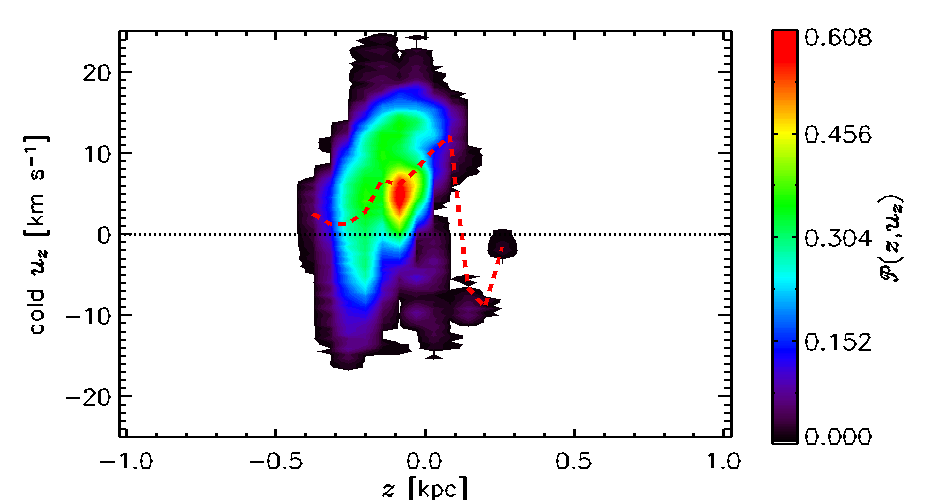
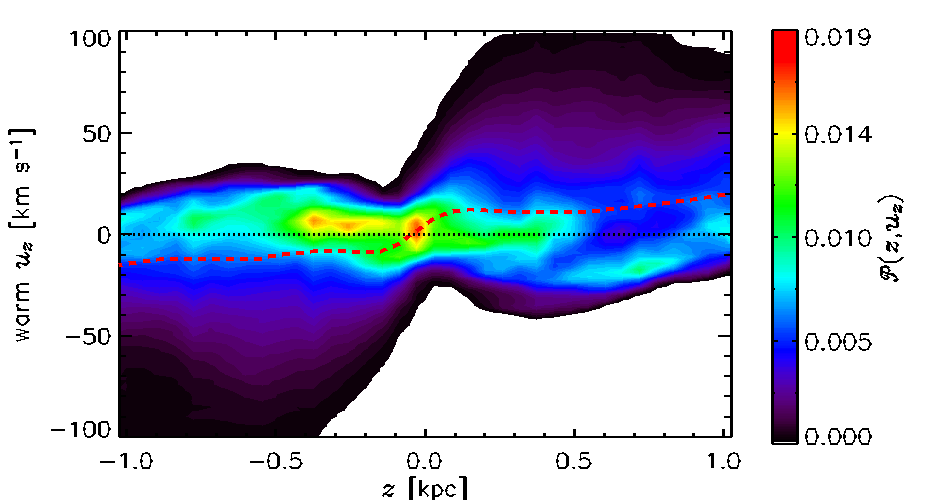
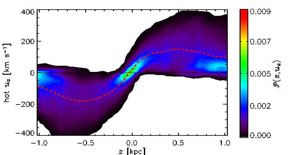
Figure 6.2: Contour plots of the probability distributions $\mathcal{P}(z,u_{z})$ for the vertical velocity $u_{z}$ as a function of $z$ in Model WSWa from eleven snapshots 634–644 Myr. The cold $(T<500\,{\rm K})$, warm $(500\,{\rm K}\leq T<5\times 10^{5}\,{\rm K})$ and hot $(T\geq 5\times 10^{5}\,{\rm K})$ are shown in panels (a) to (c), respectively. The horizontal averages of the vertical velocity $u_{z}$ in each case are over plotted (red, dashed) as well as the mid-plane position (black, dotted).

The mean vertical flow is dominated by the hot gas, so it is instructive to consider the velocity structure of each phase separately. Figure 6.2 shows plots of the probability distributions $\mathcal{P}(z,u_{z})$ as functions of $z$ and $u_{z}$ from eleven snapshots of Model WSWa, separately for the cold (a), warm (b) and hot gas (c).

The cold gas is mainly restricted to $|z|<300\,{\rm pc}$ and its vertical velocity varies within $\pm 20\,{\rm km\,s^{-1}}$ for $|z|\lessgtr 0$. On average, the cold gas moves towards the mid-plane, presumably after cooling at larger heights. The warm gas is involved in a weak net vertical outflow above $|z|=100\,{\rm pc}$, of order $\pm 10\,{\rm km\,s^{-1}}$. This might be an entrained flow within the hot gas. However, due to its skewed distribution, the modal flow is typically towards the mid-plane. The hot gas has large net outflow speeds, accelerating to about $100\,{\rm km\,s^{-1}}$ within $|z|\pm 200\,{\rm pc}$, but with small amounts of inward flowing gas at all heights. The mean hot gas outflow increases at an approximately constant rate to a speed of over $100\,{\rm km\,s^{-1}}$ within $\pm 100\,{\rm pc}$ of the mid-plane, and then decreases with further distance from the mid-plane, at a rate that gradually decreases with height for $|z|\,\hbox to0.0pt{\raise 2.15277pt\hbox{$>$}\hss}{\lower 4.30554pt\hbox{$\sim$}}\,0.5\,{\rm kpc}$. This is below the escape velocity associated with a galactic wind.

A significant effect of increased resolution is the increase in the magnitude of the perturbed velocity, from ${\langle u_{{}_{\rm rms}}\rangle}=76\,{\rm km\,s^{-1}}$ in Model WSWa to $103\,{\rm km\,s^{-1}}$ in Model WSWah (Table 4.2 Column 13) and temperatures (${\langle c{{}_{\mathrm{s}}}\rangle}$ increases from $150$ to $230\,{\rm km\,s^{-1}}$); both ${\langle u_{{}_{\rm rms}}\rangle}$ and the random velocity ${\langle u_{0}\rangle}$ are increased by a similar factor of about 1.3. However, the thermal energy $e_{\textrm{th}}$ is reduced by a factor of 0.6 with the higher resolution, while kinetic energy $e_{\textrm{K}}$ remains about the same. This suggests that in the higher-resolution model, the higher velocities and temperatures are associated with lower gas densities.

6.2 The correlation scale of the random flows

The correlation length of the random velocity $u$ at a single time step of the Model WSWa, has been estimated by calculating the second-order structure functions $\mathcal{D}(l)$ of the velocity components $u_{x}$, $u_{y}$ and $u_{z}$, where

$$\mathcal{D}(l)=\langle\left[u({{\mbox{\boldmath$x$}}}+{{\mbox{\boldmath$l$}}})-u({{\mbox{\boldmath$x$}}})\right]^{2}\rangle,$$ (6.1)

with $x$ the position in the $(x,y)$-plane and $l$ a horizontal offset. The offsets in the $z$-direction have not been included because of the systematic outflows and expected variation of the correlation length with $z$. The aggregation of the squared differences by $|{{\mbox{\boldmath$l$}}}|$, presumes that the flow is statistically-isotropic horizontally. I will consider more detailed analysis of the three-dimensional properties of the random flows, including the degree of anisotropy and its dependence on height and phase in future work.

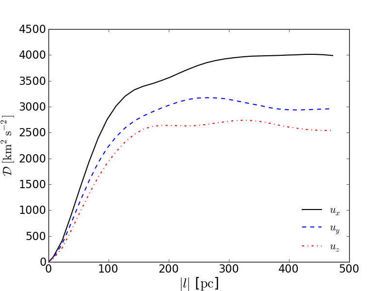
Figure 6.3: The second-order structure functions calculated using Eq. (6.1), for the layer $-10<z<10$ pc, of the velocity components $u_{x}$ (black, solid line), $u_{y}$ (blue, dashed) and $u_{z}$ (red, dash-dot). The offset $l$ is confined to the $(x,y)$-plane only.

$\mathcal{D}(l)$ was measured at five different heights, ($z=0,100,-100$, $200$ and $800\,{\rm pc}$). Averaging over six adjacent slices in the $(x,y)$-plane, each position corresponds to a layer of thickness 20 pc. The averaging took advantage of the periodic boundaries in $x$ and $y$; for simplicity choosing a simulation snapshot at a time for which the offset in the $y$-boundary, due to the shearing boundary condition, was zero. The structure function for the mid-plane ($-10<z<10\,{\rm pc}$) is shown in Fig. 6.3.

The correlation scale can be estimated from the form of the structure function since velocities are uncorrelated if $l$ exceeds the correlation length $l_{\rm turb}$, so that $\mathcal{D}$ becomes independent of $l$, $D(l)\approx 2u_{\mathrm{rms}}^{2}$ for $l\gg l_{\rm turb}$. Precisely which value of $\mathcal{D}(l)$ should be chosen to estimate $l_{\rm turb}$ in a finite domain is not always clear; for example, the structure function of $u_{y}$ in Fig. 6.3 allows one to make a case for either the value at which $\mathcal{D}(l)$ is maximum or the value at the greatest $l$. This uncertainty can give an estimate of the systematic uncertainty in the values of $l_{\rm turb}$ obtained. Alternatively, and more conveniently, one can estimate $l_{\rm turb}$ via the autocorrelation function $\mathcal{C}(l)$, related to $\mathcal{D}(l)$ by

$$\mathcal{C}(l)=1-\frac{\mathcal{D}(l)}{2u^{2}_{\mathrm{rms}}}.$$ (6.2)

In terms of the autocorrelation function, the correlation scale $l_{\rm turb}$ is defined as

$$l_{\rm turb}=\int_{0}^{\infty}\mathcal{C}(l)\,{\rm d}l,$$ (6.3)

and this provides a more robust method of deriving $l_{\rm turb}$ in a finite domain. Of course, the domain must be large enough to make $\mathcal{C}(l)$ negligible at scales of the order of the domain size; this is a nontrivial requirement, since even an exponentially small tail can make a finite contribution to $l_{\rm turb}$. In such estimates we are, of course, limited to the range of $\mathcal{C}(l)$ within the computational domain, so that the upper limit in the integral of Eq. (6.3) is equal to $L_{x}=L_{y}$, the horizontal box size; this is another source of uncertainty in the estimates of $l_{\rm turb}$.

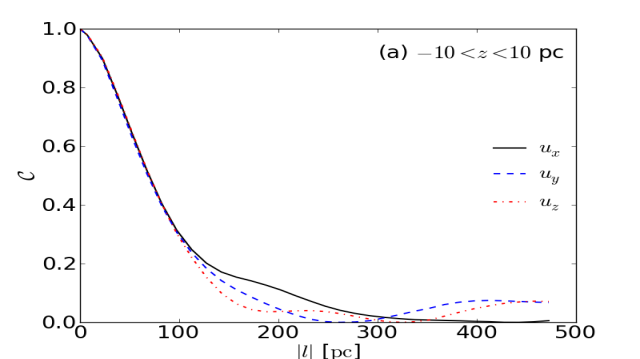
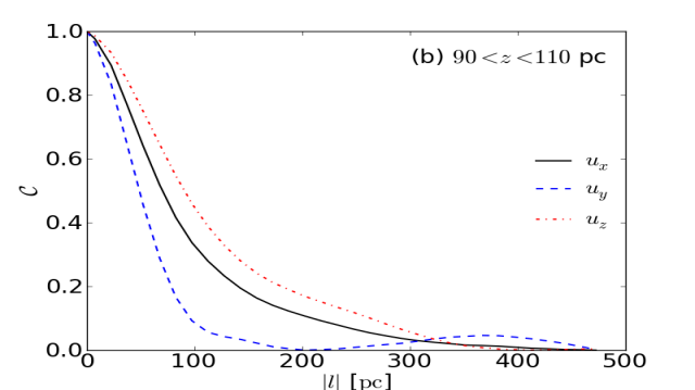
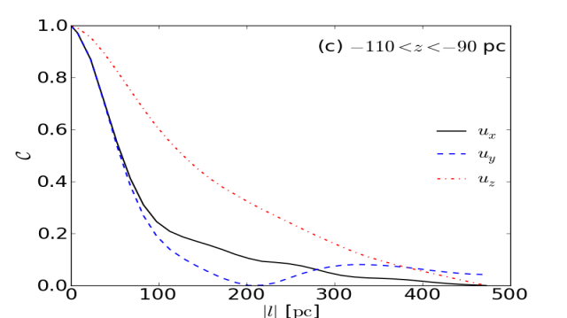
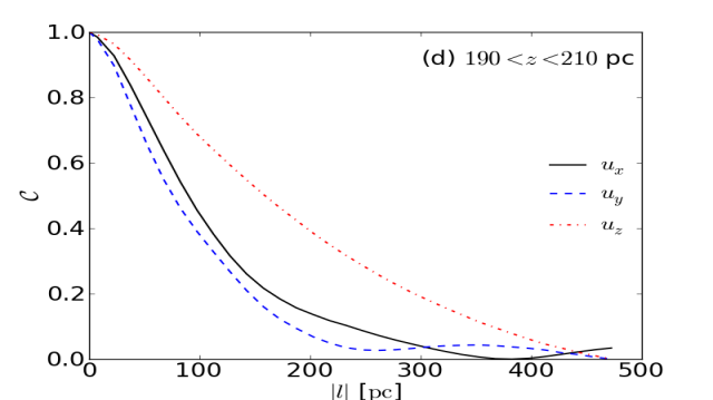
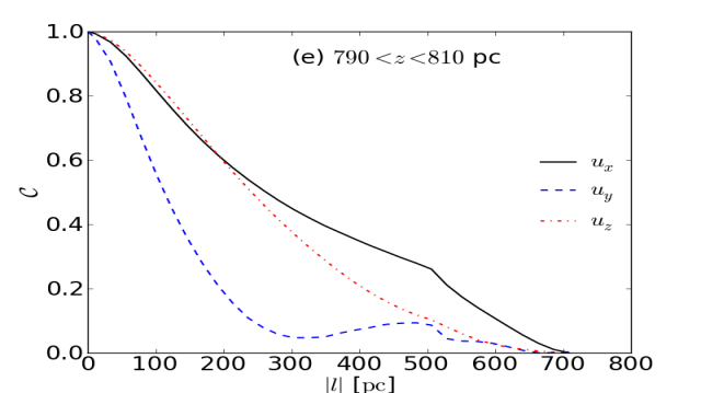
Figure 6.4: Autocorrelation functions for the velocity components $u_{x}$ (black, solid line), $u_{y}$ (blue, dashed) and $u_{z}$ (red, dash-dot) for $20\,{\rm pc}$ thick layers centred on five different heights, from top to bottom: $-10<z<10\,{\rm pc}$, $90<z<110\,{\rm pc}$, $-110<z<-90\,{\rm pc}$, $190<z<210\,{\rm pc}$ and $790<z<810\,{\rm pc}$.

Figure 6.4 shows $\mathcal{C}(l)$ for five different heights in the disc, where $u_{\mathrm{rms}}$ was taken to correspond to the absolute maximum of the structure function, $u^{2}_{\mathrm{rms}}=\max(\mathcal{D})/2$, from Eq. (6.2). The autocorrelation function of the vertical velocity varies with $z$ more strongly than, and differently from, the autocorrelation functions of the horizontal velocity components; it broadens as $|z|$ increases, meaning that the vertical velocity is correlated over progressively greater horizontal distances. Already at $|z|\approx 200\,{\rm pc}$, $u_{z}$ is coherent across a significant horizontal cross-section of the domain and at $|z|\approx 800\,{\rm pc}$ so is $u_{x}$. An obvious explanation for this behaviour is the expansion of the hot gas streaming away from the mid-plane, which thus occupies a progressively larger part of the volume as it flows towards the halo.

Table 6.1 shows the rms velocities derived from the structure functions for each component of the velocity at each height, and the correlation lengths obtained from the autocorrelation functions. Note that these are obtained without separation into phases. The uncertainties in $u_{\mathrm{rms}}$ due to the choices of local maxima in $\mathcal{D}(l)$ are less than $2\,{\rm km\,s^{-1}}$. However, these can produce quite large systematic uncertainties in $l_{\rm turb}$, as small changes in $u_{\mathrm{rms}}$ can lead to $\mathcal{C}(l)$ becoming negative in some range of $l$ (i.e. a weak anti-correlation), and this can significantly alter the value of the integral in Eq. (6.3). Such an anti-correlation at moderate values of $l$ is natural for incompressible flows; the choice of $u_{\mathrm{rms}}$ is thus not straight forward. Other choices of $u_{\mathrm{rms}}$ in Fig. 6.3 can lead to a reduction in $l_{\rm turb}$ by as much as $30\,{\rm pc}$. Better statistics, derived from data cubes for a number of different time-steps, will allow for a more thorough exploration of the uncertainties, but this analysis shall also be deferred to later work.

Table 6.1: The correlation scale $l_{\rm turb}$ and rms velocity $u_{\mathrm{rms}}$ at various distances from the mid-plane.

	$u_{\mathrm{rms}}$ [$\!\,{\rm km\,s^{-1}}$]				$l_{\rm turb}$ [$\!\,{\rm pc}$]
$z$	$u_{x}$	$u_{y}$	$u_{z}$		$u_{x}$	$u_{y}$	$u_{z}$
$\phantom{-10}0$	$45$	$40$	$37$		$99$	$98$	$94$
$\phantom{-}100$	$36$	$33$	$43$		$102$	$69$	$124$
$-100$	$39$	$50$	$46$		$95$	$87$	$171$
$\phantom{-}200$	$27$	$20$	$63$		$119$	$105$	$186$
$\phantom{-}800$	$51$	$21$	$107$		$320$	$158$	$277$

The rms velocities given in Table 6.1 are compatible with the global values of $u_{\mathrm{rms}}$ and $u_{\rm turb}$ for the reference run W$\Omega$ shown in Table 4.1 (within their uncertainties). The increase in the root-mean-square value of $u_{z}$ with height, from about $40\,{\rm km\,s^{-1}}$ at $z=0$ to about $60\,{\rm km\,s^{-1}}$ at $z=200\,{\rm pc}$, reflects the systematic outflow with a speed increasing with $|z|$. There is also an apparent tendency for the root-mean-square (rms) values of $u_{x}$ and $u_{y}$ to decrease with increasing distance from the mid-plane. This is understandable, as the rate of acceleration from SN forcing will decline from the mid-plane. However it is not excluded that these rms values might increase again at heights substantially away from the mid-plane, where the gas is hotter and gas speeds are generally higher in all directions.

The correlation scale of the random flow is very close to $100\,{\rm pc}$ in the mid-plane, and this value has been adopted for $l_{\rm turb}$ elsewhere in the thesis. This estimate is in good agreement with the hydrodynamic ISM simulations of Joung and Mac Low (2006), who found that most kinetic energy is contained by fluctuations with a wavelength (i.e. $2l_{\rm turb}$ in our notation) of $190\,{\rm pc}$. In the MHD simulations of Korpi, Brandenburg, Shukurov, Tuominen and Nordlund (1999), $l_{\rm turb}$ for the warm gas was $30\,{\rm pc}$ at all heights, but that of the hot gas increased from $20\,{\rm pc}$ in the mid-plane to $60\,{\rm pc}$ at $|z|=150\,{\rm pc}$. de Avillez and Breitschwerdt (2007) found $l_{\rm turb}=73\,{\rm pc}$ on average, with strong fluctuations in time. As in Korpi, Brandenburg, Shukurov, Tuominen and Nordlund (1999), there is a weak tendency for $l_{\rm turb}$ of the horizontal velocity components to increase with $|z|$ in my simulations, but this tendency remains tentative, and must be examined more carefully to confirm whether it is robust. The correlation scale of the vertical velocity, which has a systematic part due to the net outflow of hot gas, grows from about $100\,{\rm pc}$ at the mid-plane to nearly $200\,{\rm pc}$ at $z=200\,{\rm pc}$. Due to the increase of the fractional volume of the hot gas with distance from the mid-plane, this scale might be expected also to increase further.

6.3 Summary

The heating and shocking induced by SNe produce a mean outflow of gas from the disc of up to $200\,{\rm km\,s^{-1}}$ within $|z|\,\hbox to0.0pt{\raise 2.15277pt\hbox{$<$}\hss}{\lower 4.30554pt\hbox{$\sim$}}\,500\,{\rm pc}$, which slows to $100\,{\rm km\,s^{-1}}$ within $|z|\,\hbox to0.0pt{\raise 2.15277pt\hbox{$<$}\hss}{\lower 4.30554pt\hbox{$\sim$}}\,1\,{\rm kpc}$, which is mainly comprised of hot gas. These velocities are below the escape velocity, that would be associated with a galactic wind, so represents only the outward part of the galactic fountain. The horizontal correlation scale of the turbulent flow is of order $100\,{\rm pc}$ near the mid-plane. The correlation length increases with height, reaching $200$–$300\,{\rm pc}$ for $|z|\simeq 800\,{\rm pc}$, and likely to continue to increase above this.

Chapter 7 Sensitivity to model parameters

7.1 Sensitivity to the cooling function

An important factor in the persistence of a multi-phase ISM is the action of differential cooling. Radiative cooling and UV-heating rates in the ISM are dependent on a variety of localised factors, such as gas density, the presence and abundance of helium, heavier elements and metals, filtering by dust grains, and the temperature and ionization of the gas (Wolfire et al., 1995). In simulations of this kind, where the gas is usually modelled as a single fluid with a mean molecular weight, the cooling and heating processes are heavily parametrized. Many authors adopt alternative cooling profiles, with little effort to establish the utility of their choice. Some comparisons have been recorded between cooling functions, but using alternative numerical methods or modelling indirectly related physical problems. de Avillez and Breitschwerdt (2010) use a time dependent cooling function, which recognises the delay in recombination of previously ionized gas, and demonstrates that there is a substantial variation in the resulting cooling. There are inevitably overheads associated with this refinement. So far, the extent to which this affects the primary global properties of the ISM (temperature, density, velocity distributions) has not been clarified.

Here two models, RBN and WSWb, with parameters given in Table 4.1, are compared directly to assess how the specific choice of the cooling functions affect the results. Apart from different parameterizations of the radiative cooling, the two models share identical parameters, except as follows: because of the sensitivity of the initial conditions to the cooling function (Section 3.6), the value of $T_{0}$ was slightly higher in Model RBN. (The density, heating and gravity profiles were the same.)

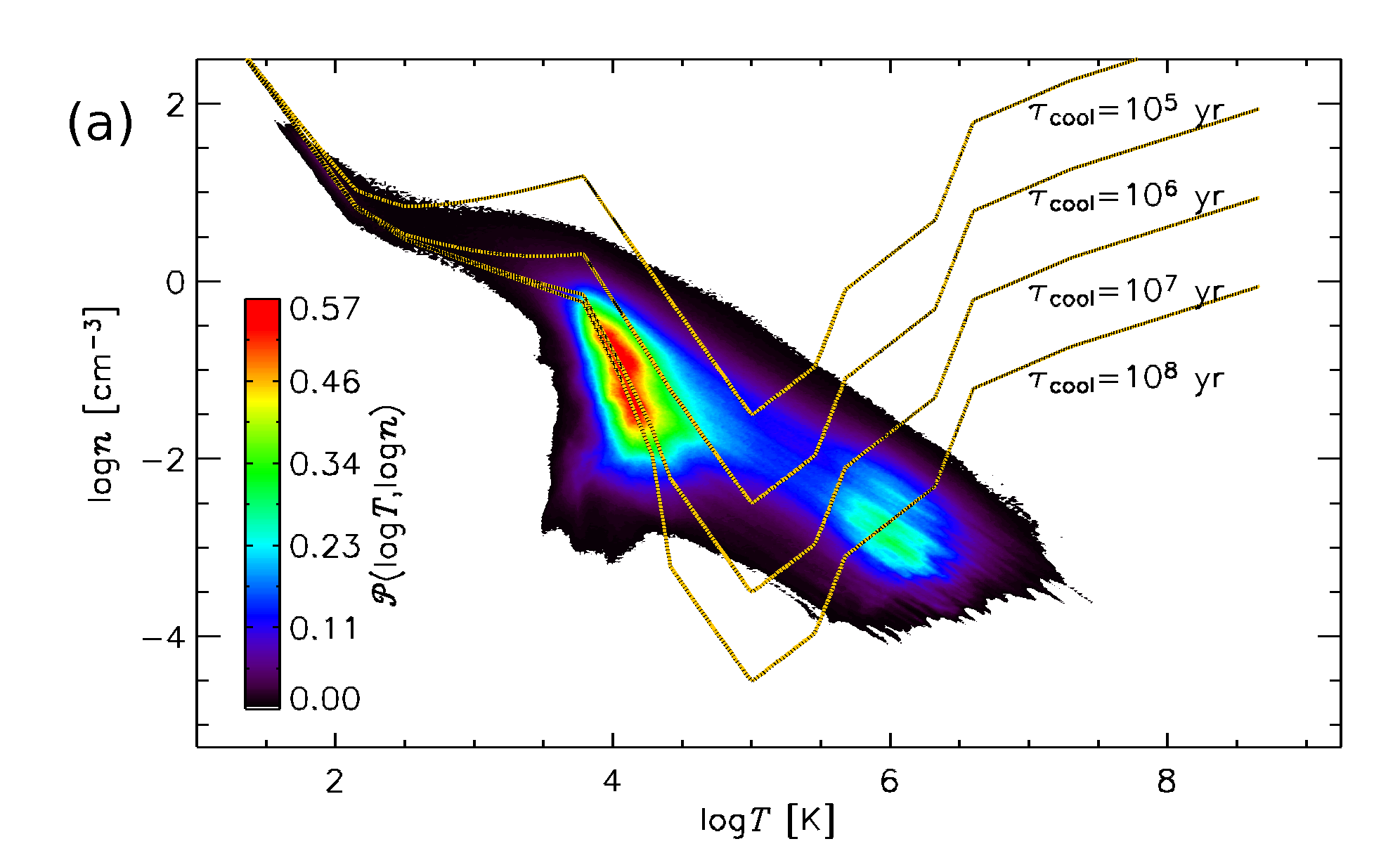
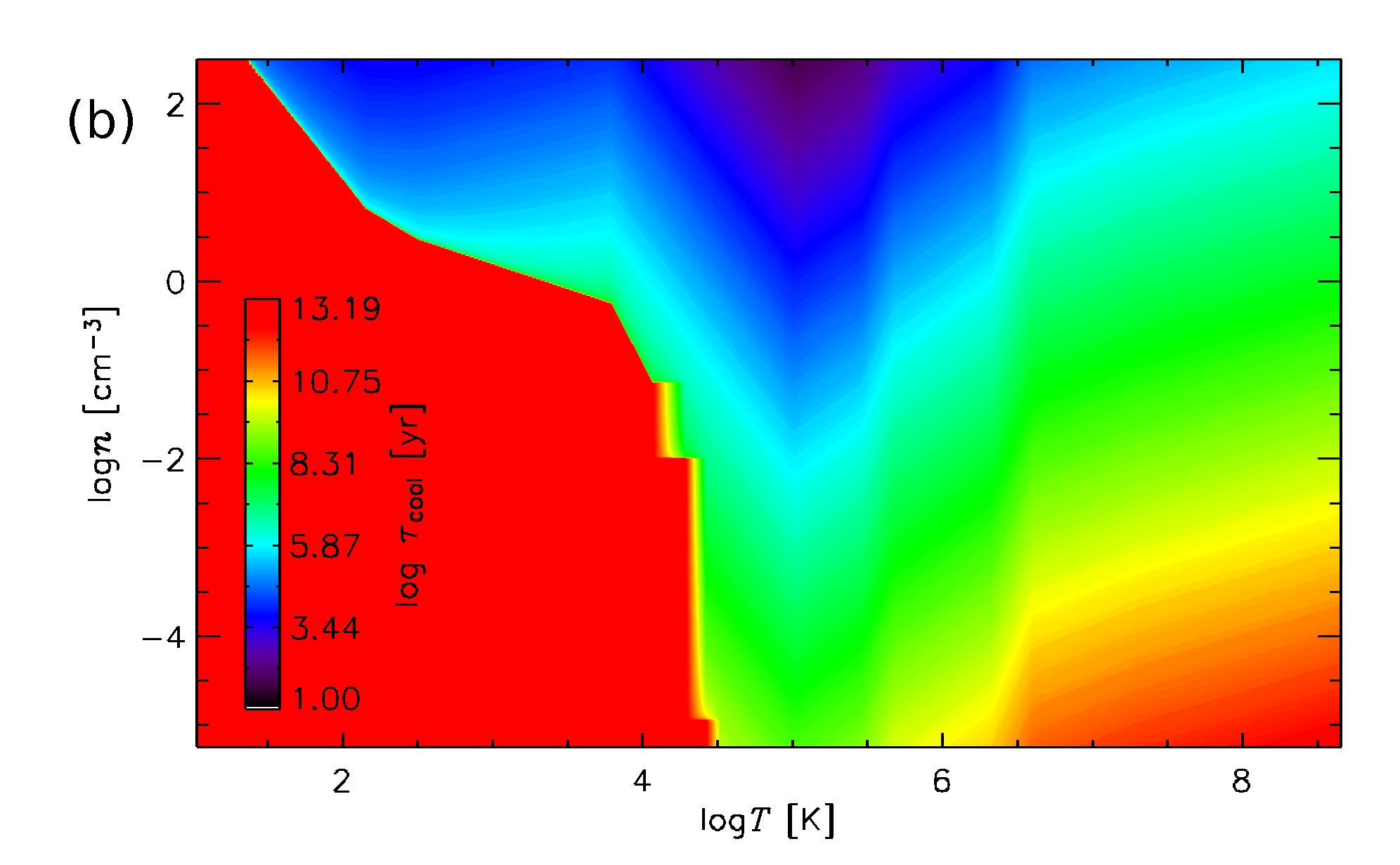
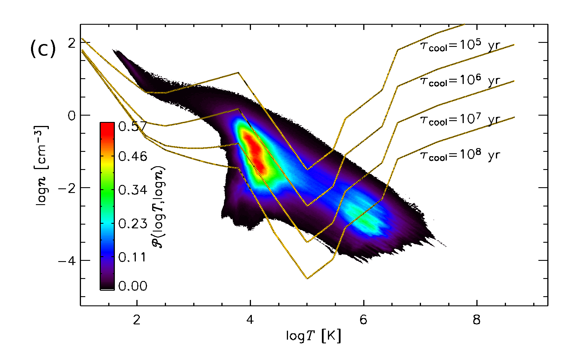
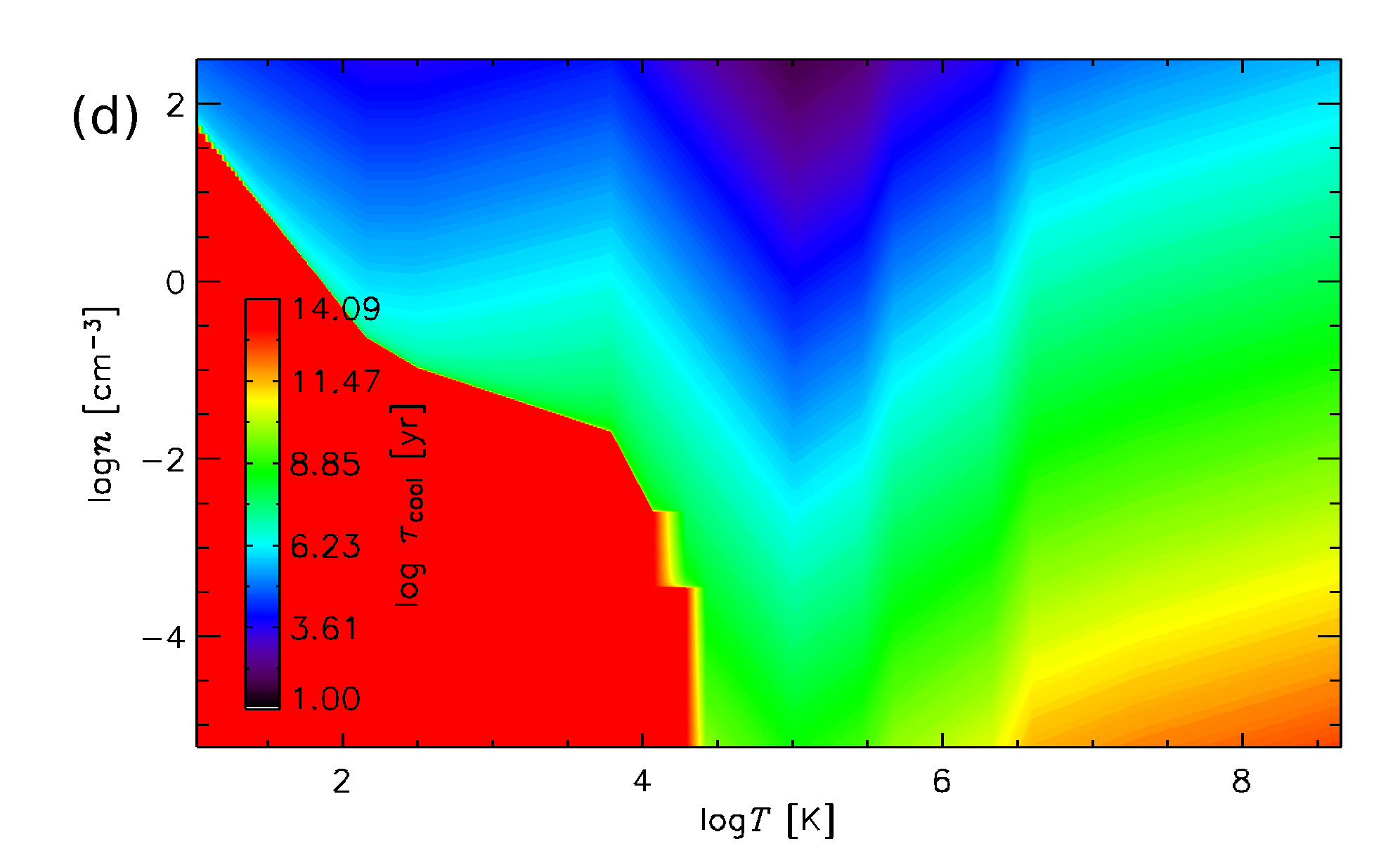
Figure 7.1: (a) The total volume probability distributions by gas number density $n$ and temperature $T$. Eleven snapshots of Model WSWb in the interval $t=305$ to $325\,{\rm Myr}$ were used, with the system in a statistical steady state. Contours of constant cooling time ($10^{5},~{}10^{6},~{}10^{7}$ and $10^{8}$yr) are over plotted to indicate where the gas may be subject to rapid radiative cooling. These are drawn from the contour plot of cooling time $\tau{{}_{\rm cool}}$ (b), given in Eq. (7.1) with diffuse heating $\Gamma(0)$ as applied at the mid-plane $z=0$. The solid red patch at $T\,\hbox to0.0pt{\raise 2.15277pt\hbox{$<$}\hss}{\lower 4.30554pt\hbox{$\sim$}}\,10^{4}\,{\rm K}$ is a region where heating exceeds cooling so $\tau{{}_{\rm cool}}$ is not defined. In (c) and (d) the contours again as (a) and (b) respectively, but for $\Gamma(z)$ at $|z|=1\,{\rm kpc}$.

One consideration with the inclusion of a thermally unstable branch for the WSW cooling function, used in Model WSWa, is that the cooling times must be adequately resolved (see Section 3.4 and Appendix B.2). From Eq. (3.1), the net cooling rate due to the diffuse heating and cooling terms is

$$\frac{Ds}{Dt}=-\left(\frac{\rho\Gamma(z)-\rho^{2}\Lambda}{\rho T}\right);\quad[({\mathrm{in~{}cgs~{}units}})~{}~{}\,{\rm erg}\,{\rm g}^{-1}\,{\rm K}^{-1}\,{\rm s}^{-1}].$$

The cooling time $\tau{{}_{\rm cool}}$ is then given by

$$\tau{{}_{\rm cool}}=\frac{\,{c_{\rm v}}T}{\rho\Lambda-\Gamma(z)}\quad[\,{\rm s}\,],$$ (7.1)

where $\Lambda$ and $\Gamma$ are the radiative cooling and ultra violet heating respectively, as described in Section 3.3, and $\,{c_{\rm v}}$ is the specific heat capacity of the gas at constant volume.

In Fig. 7.1a the combined probability distributions of the gas number density and temperature in Model WSWb are overplotted with contours of constant cooling time $\tau{{}_{\rm cool}}$, from the WSW cooling function and with the heating as it is applied at the mid-plane. Alongside this (Fig. 7.1b) are the contours of $\tau{{}_{\rm cool}}$ for the same range of temperature and density as in panel a. Note that the distribution in panel a is considerably broader than that for Model WSWa, displayed in Fig 5.4; i.e. there is greater pressure dispersion associated with the additional mass included in Models WSWb and RBN.

The heating $\Gamma(z)$ is a maximum at the mid-plane and reduces with $|z|$. Ultra violet heating only applies at temperatures up to about $2\cdot 10^{4}\,{\rm K}$, so $\tau{{}_{\rm cool}}$ is independent of $z$ above these temperatures. Below $T\simeq 10^{4}\,{\rm K}$ there are densities where heating exceeds cooling, so the cooling time is undefined, indicated by the solid red regions in the contour plot (b). From (a) it is apparent that the distribution of the cold gas is bounded by this region, suggesting that gas cannot remain cold as it is reheated very quickly. The very narrow distribution of the cold gas is in part explained by the equivalently narrow ‘corridor’ between the rapid heating (red) and the rapid cooling (blue) bounding it.

The effect of reduced heating with height is illustrated by the revised contours of $\tau{{}_{\rm cool}}$ (Fig. 7.1 c,d) for $|z|=1\,{\rm kpc}$. The corridor between rapid heating and rapid cooling shifts well below the location of the cold gas in panel (c). It is also the case that the density of the gas reduces with height. Therefore negligible quantities of gas in the thermally unstable range $313$–$6102\,{\rm K}$ will be subject to this faster cooling and longer cooling times near the mid-plane will apply.

Only warm gas $T\simeq 10^{5}\,{\rm K}$ is significantly subject to cooling times less than $10^{5}\,{\rm yr}$. There exists a substantial distribution of warm gas $T\simeq 10^{4}\,{\rm K}$ inside the (red) region where $\Gamma(0)>\rho\Lambda$ (panel a), but not so for $\Gamma(1)$ (b). From inspection of the distribution of gas near the mid-plane (Fig. 7.3a below) it is clear that very little gas occupies the region of net heating (solid, red). Some gas below $10^{4}\,{\rm K}$ does spread into this region indicating that adiabatic cooling due to compression and expansion is dominant here.

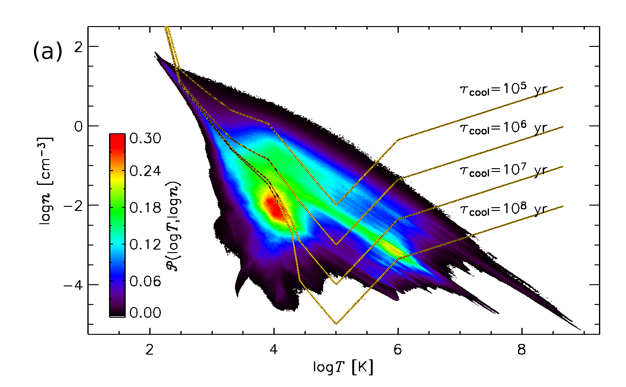
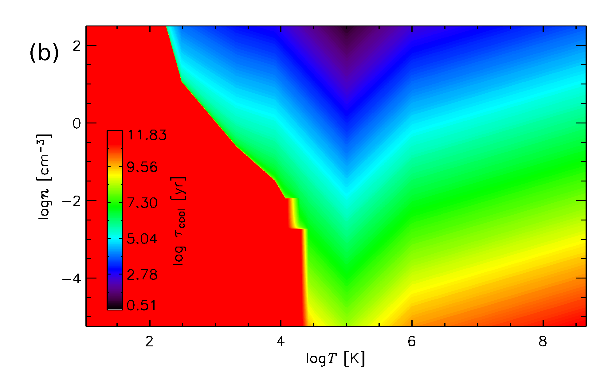
Figure 7.2: (a) The total volume probability distributions by gas number density $n$ and temperature $T$ for Model RBN. Contours of constant cooling time ($10^{5},~{}10^{6},~{}10^{7}$ and $10^{8}$yr) are over plotted to indicate where the gas may be subject to rapid radiative cooling. These are drawn from the contour plot of cooling time $\tau{{}_{\rm cool}}$ (b), given in Eq. (7.1) with diffuse heating $\Gamma(0)$ as applied at the mid-plane $z=0$. The solid red patch at $T\,\hbox to0.0pt{\raise 2.15277pt\hbox{$<$}\hss}{\lower 4.30554pt\hbox{$\sim$}}\,10^{4}\,{\rm K}$ is a region where heating exceeds cooling so $\tau{{}_{\rm cool}}$ is not defined.

In Fig. 7.2, panels a and b of Fig. 7.1 are reproduced for Model RBN. There is far more gas in the temperature range around $10^{3}\,{\rm K}$, due to the absence of a thermally unstable branch between 313 and $6102\,{\rm K}$. The distribution of the cold gas near $\log n\simeq\log T\simeq 2$ is very similar to Model WSWb (Fig. 7.1a,c), although in this case it is not aligned with the narrow corridor between rapid heating (red) and rapid cooling (blue, panel b). This indicates that the composition of the cold gas is strongly dependent on the adiabatic shocks, rather than the balance between heating and cooling processes. The corresponding contours of $\tau{{}_{\rm cool}}$ extend to much lower densities in the temperature range above $10^{6}\,{\rm K}$, so cooling times are much shorter for RBN cooling. Yet there is a greater abundance of very hot gas than with Model WSWb, which is explained by the much lower density of this gas, which mitigates against the tendency for rapid cooling.

The distributions of gas near the mid-plane (within $100\,{\rm pc}$) for both models are displayed in Fig. 7.3. From these it is evident that the low temperature – low density boundary of the distributions aligns quite strongly with the region of net heating (red in Fig. 7.1b and Fig. 7.2b), although there is limited dispersion into this region. Both models have distributions with extended peaks along this boundary below $10^{3}\,{\rm K}$, corresponding to the most thermally stable location. This extends to higher temperature for RBN cooling than for WSW, through the range which is unstable for the latter. However the most significant alignment, common to both models, is along the line of constant thermal pressure. Note that the colour scale differs between the plots, such that these peaks contain a similar proportion of the gas in both models. The cold dense tip of the RBN distribution extends into the region ($\log n\simeq\log T\simeq 2$) where net heating should make it unstable, yet lies on the line of constant pressure through the peaks of warm and hot gas. This is associated with the equilibrium pressure between the phases, which is slightly lower at the mid-plane for WSW cooling than for RBN. In contrast to the case for the total volumes, Model WSWb has more gas near the mid-plane at higher temperature and lower density than Model RBN. Beyond this the cooling function has only a weak effect on the distribution for the gas with $T\,\hbox to0.0pt{\raise 2.15277pt\hbox{$>$}\hss}{\lower 4.30554pt\hbox{$\sim$}}\,10^{3}\,{\rm K}$.

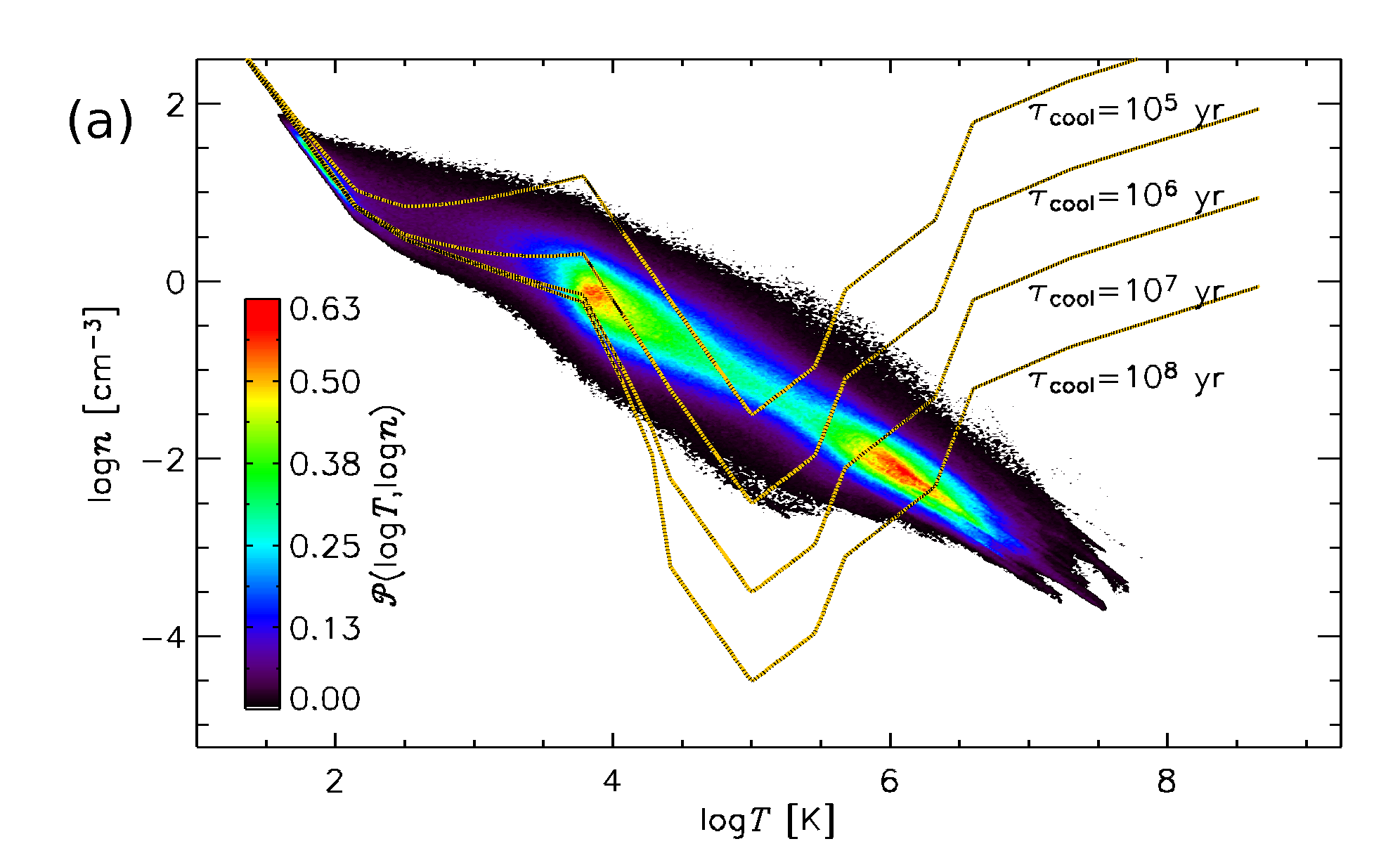
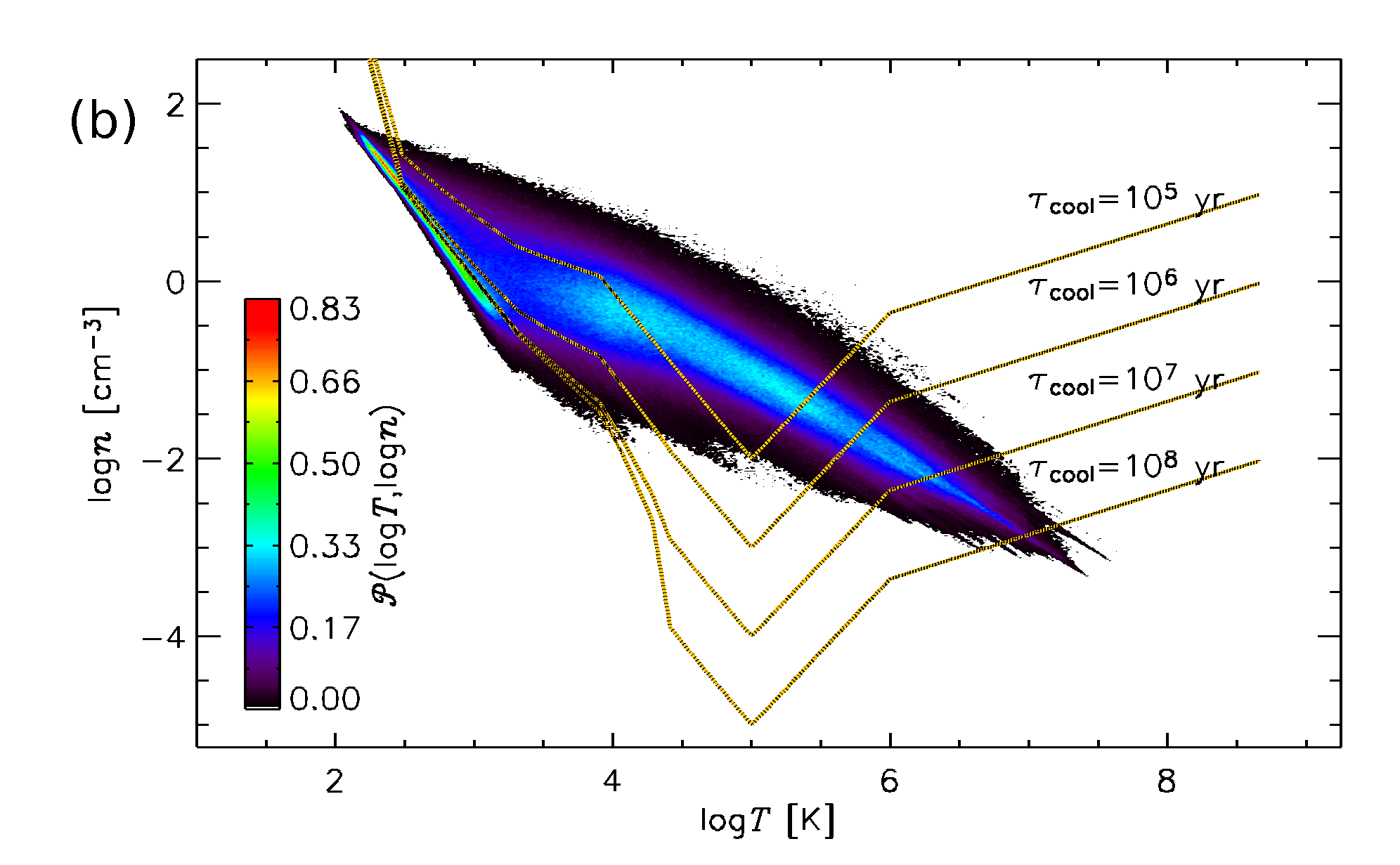
Figure 7.3: The mid-plane probability distributions ($|z|<100\,{\rm pc}$) by gas number density $n$ and temperature $T$ for (a) Model WSWb and (b) Model RBN. Contours of constant cooling time ($10^{5},~{}10^{6},~{}10^{7}$ and $10^{8}$yr) are over plotted to indicate where the gas may be subject to rapid radiative cooling.

The volume-averaged thermal and kinetic energy densities, the latter due to the perturbed motions alone, are shown in Fig. 7.4 as functions of time. The averages for each are shown in Columns 15 and 16, respectively of Table 4.2, using the appropriate steady state time intervals given in Column 18. Models reach a statistically steady state, with mild fluctuations around a well defined mean value, very soon (within 60 Myr of the start of the simulations). The effect of the cooling function is evident: both the thermal and kinetic energies in Model RBN are about 60% of those in Model WSWb. This is understandable as Model RBN has a stronger cooling rate than Model WSWb, only dropping below the WSW rate in the range $T<10^{3}\,{\rm K}$ (see Fig. 3.1).

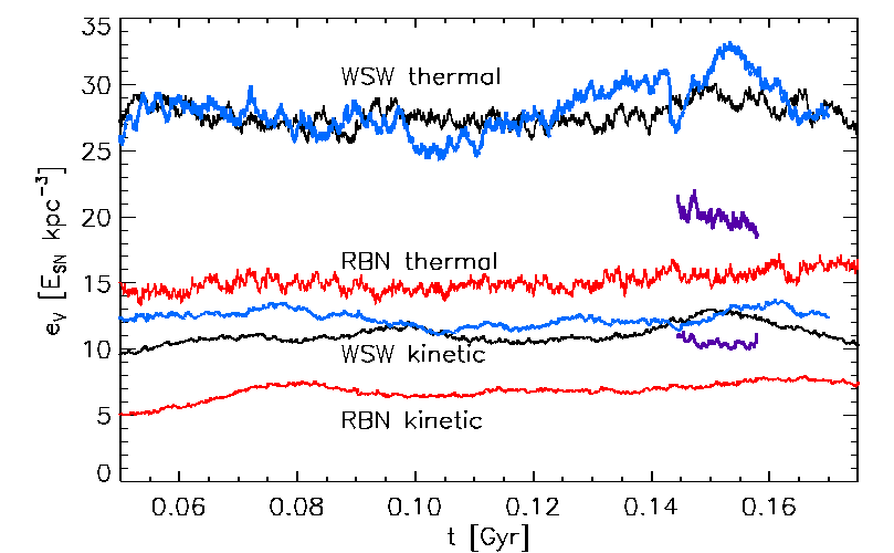
Figure 7.4: Evolution of volume-averaged thermal (black: Model WSWb, blue: Model WSWa, purple: Model WSWah, red: Model RBN) and kinetic energy density (lower lines) in the statistically steady regime, normalised to the SN energy $E_{\rm SN}\,{\rm kpc}^{-3}$. Models WSWb (black) and RBN (red) essentially differ only in the choice of the radiative cooling function.

Interestingly, both models are similar in that the thermal energy is about $2.5$ times the kinetic energy. These results are remarkably consistent with results by Balsara et al. (2004, their Fig. 6) and Gressel (2008, Fig. 3.1). Gressel (2008) applies WSW cooling and has a model very similar to Model WSWa, but with half the resolution and $|z|\leq 2\,{\rm kpc}$. He reports average energy densities of 24 and 10 $E_{\rm SN}\,{\rm kpc}^{-3}$ (thermal and kinetic, respectively) with SN rate $\dot{\sigma}_{\rm SN}$, comparable to 29 and 13 $E_{\rm SN}\,{\rm kpc}^{-3}$ obtained here for Model WSWa.

Balsara et al. (2004) simulate an unstratified cubic region $200\,{\rm pc}$ in size, driven at SN rates of 8, 12 and 40 times the Galactic rate, with resolution more than double that of Model WSWa. For SN rates $12\dot{\sigma}_{\rm SN}$ and $8\dot{\sigma}_{\rm SN}$, they obtain average thermal energy densities of about 225 and 160$\,E_{\rm SN}\,{\rm kpc}^{-3}$, and average kinetic energy densities of 95 and 60$\,E_{\rm SN}\,{\rm kpc}^{-3}$, respectively (derived from their energy totals divided by the $[200\,{\rm pc}]^{3}$ volume).

To allow comparison with models here, where the SNe energy injection rate is $1\dot{\sigma}_{\rm SN}$, we divide their energy densities by 12 and 8, respectively, to obtain energy densities of 19 and 20 $E_{\rm SN}\,{\rm kpc}^{-3}$ (thermal), and 8 and 7.5 $E_{\rm SN}\,{\rm kpc}^{-3}$ (kinetic). These are slightly smaller than our results with RBN cooling (25 and 9 $E_{\rm SN}\,{\rm kpc}^{-3}$) and those with WSW (29 and 13 $E_{\rm SN}\,{\rm kpc}^{-3}$ for WSWa, as given above). Since Balsara et al. (2004) used an alternative cooling function (Raymond and Smith, 1977), leading to some additional uncertainty over the net radiative energy losses, the results appear remarkably consistent.

While cooling and resolution may marginally affect the magnitudes, it appears that the thermal energy density may consistently be expected to be about $2.5$ times the kinetic energy density, independent of the model. It also appears, from comparing the stratified and unstratified models, that the ratio of thermal to kinetic energy is not strongly dependent on height, at least between the mid-plane and $\pm 2\,{\rm kpc}$.

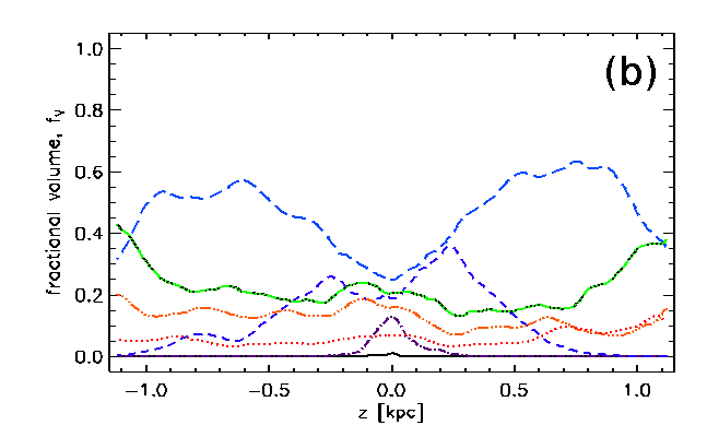
Figure 7.5: Vertical profiles of the fractional volumes occupied by the various temperature ranges, with the key shown in Table 7.1. (a) Model WSWb, using 21 snapshots spanning 305 to 325 Myr. (b) Model RBN, using 21 snapshots spanning 266 to 286 Myr.

Figure 7.5, which plots the horizontal fractional volumes $f_{V,i}(z)$ defined in Eq. (5.16), helps reveal how the thermal gas structure depends on the cooling function. Model WSWb, panel (a), has significantly more very cold gas ($T<50\,{\rm K}$; black, solid) than RBN, panel (b), but slightly warmer cold gas ($T<500\,{\rm K}$; purple, dash-dotted) is more abundant in RBN. The warm and hot phases ($T>5\times 10^{3}\,{\rm K}$) have roughly similar distributions in both models, although Model RBN has less of both phases. Apart from relatively minor details, the effect of the form of the cooling function thus appears to be straightforward and predictable: stronger cooling means more cold gas, and vice versa. What is less obvious, however, is that the very hot gas is more abundant near $\pm 1\,{\rm kpc}$ in Model RBN than in WSWb, indicating that the typical densities must be much lower. This, together with the greater abundance of cooler gas near the mid-plane, suggest that there is less stirring with RBN cooling.

Table 7.1: Key to Figs. 5.12 and 7.5, defining the gas temperature bands used there (same as Table 5.2).

Temperature band	Line style	Phase
$5\times 10^{1}\,{\rm K}<$$T<5\times 10^{1}\,{\rm K}$		cold
$5\times 10^{1}\,{\rm K}\leq T<5\times 10^{2}\,{\rm K}$	$\cdot$-$\cdot$-$\cdot$-$\cdot$-$\cdot$	cold
$5\times 10^{2}\,{\rm K}\leq T<5\times 10^{3}\,{\rm K}$	- - - - -	warm
$5\times 10^{3}\,{\rm K}\leq T<5\times 10^{4}\,{\rm K}$	– – – -	warm
$5\times 10^{4}\,{\rm K}\leq T<5\times 10^{5}\,{\rm K}$	–- $\cdot$- $\cdot$- –	warm
$5\times 10^{5}\,{\rm K}\leq T<5\times 10^{6}\,{\rm K}$	–$\cdots$–$\cdot$	hot
$5\times 10^{1}\,{\rm K}<$$T\geq 5\times 10^{6}\,{\rm K}$	$\cdots\cdots$	hot

The two models are further compared in Fig. 7.6, where separate probability distributions are shown for the gas density, temperature and thermal pressure. With both cooling functions, the most probable gas number density is around $3\times 10^{-2}\,{\rm cm}^{-3}$; the most probable temperatures are also similar, at around $3\times 10^{4}\,{\rm K}$. With the RBN (blue, dashed) cooling function, the density range extends to smaller densities than with WSWb (black, solid); on the other hand, the temperature range for WSWb extends both lower and higher than for RBN. It is evident that the isobarically unstable branch of WSW cooling significantly reduces the amount of gas in the 313–6102 K temperature range (dark blue, dashed in Fig. 7.5) and increases the amount below 100 K. However this is not associated with higher densities than RBN. This may be indicative that multiple compressions, rather than thermal instability, dominate the formation of dense clouds. The most probable thermal pressure is lower in Model RBN than in WSWb, consistent with the lower thermal energy content of the former, and with the differences between the 2D plots in Fig. 7.1a (WSW) and Fig. 7.2a (RBN). However, in contrast, the pressure at the mid-plane (Fig. 7.3) is higher for Model RBN than for Model WSWb.

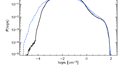
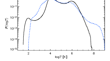
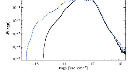
Figure 7.6: Volume weighted probability distributions for (a) gas density, (b) temperature and (c) thermal pressure, for Model RBN (blue, dashed) and Model WSWb (black, solid), in a statistical steady state, each averaged over 21 snapshots spanning 20 Myr (RBN: 266 to $286\,{\rm Myr}$, and WSWb: 305 to $325\,{\rm Myr}$) and the total simulation domain $|z|\leq 1.12\,{\rm kpc}$.

The density and temperature probability distributions for WSWb are similar to those obtained by Joung and Mac Low (2006, their Fig. 7), who used a similar cooling function, despite the difference in the numerical methods (adaptive mesh refinement down to $1.95\,{\rm pc}$ in their case). With slightly different implementation of the cooling and heating processes, again with adaptive mesh refinement down to $1.25\,{\rm pc}$, de Avillez and Breitschwerdt (2004, their Fig. 3) found significantly more cool, dense gas. It is noteworthy that the maximum densities and lowest temperatures obtained in my study with a non-adaptive grid are of the same order of magnitude as those from AMR-models, where the local resolution is up to three times higher. At $4\,{\rm pc}$ resolution, the mean minimum temperature is $34\,{\rm K}$, within the range $15$–$80\,{\rm K}$ for 0.625–$2.5\,{\rm pc}$ (de Avillez and Breitschwerdt, 2004, their Fig. 9). For mean maximum gas number, my value of $122\,{\rm cm^{-3}}$ is within their range $288$–$79\,{\rm cm^{-3}}$.

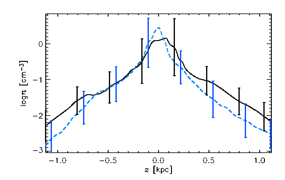
Figure 7.7: Horizontal averages of gas number density, $\overline{n}(z)$, for Model WSWb (solid, black) and Model RBN (dashed, blue). Each are time-averaged using eleven snapshots. The vertical lines indicate standard deviation within each horizontal slice.

In Fig 7.7 the horizontal averages of the gas number density $n$ are plotted for Models WSWb (black) and RBN (blue). The density scale height is lower for Model RBN, indicative that the stronger cooling is inhibiting the circulation of hot gas away from the mid-plane.

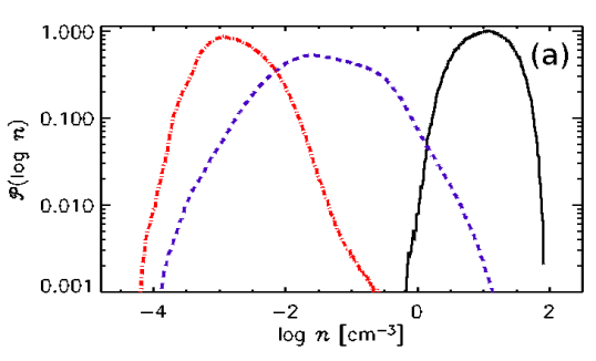
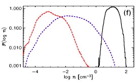
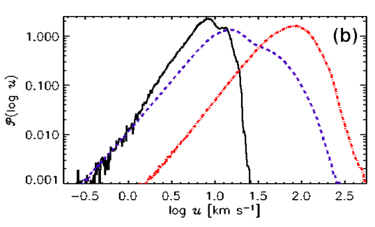
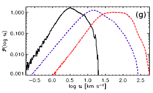
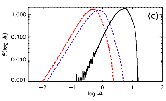
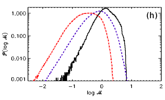
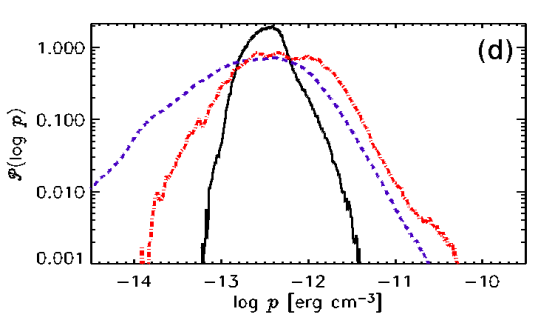
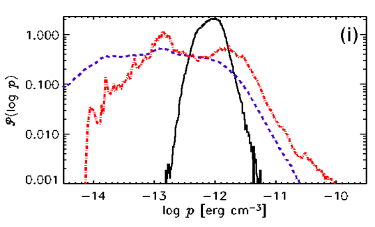
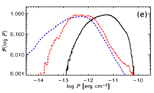
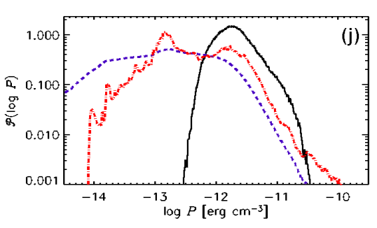
Figure 7.8: Total volume phase probability distributions for Model WSWb (left column) and Model RBN (right column): gas number density $n$ (a),(f); turbulent velocity $u_{\rm turb}$ (b),(g); Mach number defined with respect to local sound speed and $u_{\rm turb}$ (c),(h); thermal pressure (d),(i); and total pressure (e),(j). Cold phase $T<500\,{\rm K}$ (black, solid), warm $500<T<5\times 10^{5}\,{\rm K}$ (blue, dashed) and hot $T>5\times 10^{5}\,{\rm K}$ (red, dash-dotted). Eleven snapshots have been used for averaging, spanning $t=266$ to $286\,{\rm Myr}$ for Model RBN and $t=305$ to $325\,{\rm Myr}$ for Model WSWb.

The probability distributions of Fig. 7.6 do not show clear separations into phases (cf. the distributions shown by Joung and Mac Low (2006); de Avillez and Breitschwerdt (2004)); thus division into three phases would arguably only be conventional, if based on these distributions alone. Based on the analysis described in Section 5.1, however the assertion that the complicated thermal structure can indeed be reasonably described in terms of three phases remains justified.

Distributions of density obtained for the individual phases from Models WSWb and RBN, shown in Fig. 7.8a and f respectively, confirm the clear phase separation in both cases. This is also clear from the perturbation velocity in Fig 7.8b and g. Here the same borderline temperatures are defined for individual phases as for Model WSWa (Fig. 5.5). Despite minor differences between the corresponding panels in Figs. 5.5 and 7.8, the peaks in the gas density probability distributions are close to $10^{1},3\times 10^{-2}$ and $10^{-3}\,{\rm cm}^{-3}$ in all models. The similarity in the properties of the cold gas suggests that the radiative cooling (different in Models RBN and WSW) is less important than adiabatic cooling at these scales. Given the extra cooling of hot gas and reduced cooling of cold gas with the RBN cooling function, more of the gas resides in the warm phase in Model RBN. The probability distribution for the Mach number in the warm gas extends to higher values with the RBN cooling function, perhaps because more shocks reside in the more widespread warm gas, at the expense of the cold phase. It is useful to remember that, although each distribution in this figure is normalised to unit underlying area, the fractional volume of the warm gas is about a hundred times that of the cold.

The thermal pressure distribution in the hot gas reveals the two ‘types’ (see the end of section 5.1), which are mostly found within $|z|\,\hbox to0.0pt{\raise 2.15277pt\hbox{$<$}\hss}{\lower 4.30554pt\hbox{$\sim$}}\,200\,{\rm pc}$ (high pressure hot gas within SN remnants) and outside this layer (diffuse, lower pressure hot gas). The broader pressure distributions in both models, as compared to Fig. 5.5, indicate that the enhanced mass, particularly in the SN active regions, adds resistance to the release of hot gas from the mid-plane through blow outs and convection. The pressure builds up at the mid-plane without release to the halo, leading to a stronger vertical pressure gradient. This is also evident in the MHD models (Sections 7.2 and 9), where the circulation of hot gas out of the disc is partially inhibited by the presence of a predominantly horizontal magnetic field. Note that the location of the cold gas thermal pressure (Fig. 7.8i) is offset from the hot pressure peak, but for total pressure (panel j) they are well aligned.

In conclusion, the properties of the cold and warm phases are not strongly affected by the choice of the cooling function. The main effect is that the RBN cooling function produces slightly less hot gas, but extended to higher temperatures with significantly lower pressures. This can readily be understood, as this function provides significantly stronger cooling at $T\,\hbox to0.0pt{\raise 2.15277pt\hbox{$>$}\hss}{\lower 4.30554pt\hbox{$\sim$}}\,10^{3}\,{\rm K}$.

7.2 Sensitivity to rotation, shear and SN rate

More thorough analysis of the effects of the other model parameters included here will need to follow in future work. Direct comparison between Models ${\mathrm{B}2\rm{\Omega}}$ and ${\mathrm{B}1\rm{\Omega}}$ in the saturated state may be used to consider the effect of rotation, but further studies with reduced rotation and a range of rotation rates would be more informative. The effects of shear and supernova rate can only be directly considered in the kinematic stage for the MHD runs with Models ${\mathrm{B}1\rm{\Omega}\rm{SN}}$ and ${\mathrm{B}1\rm{\Omega}\rm{Sh}}$, and it would also be helpful to consider a range of these parameters, to get a fuller appreciation of their effects.

From Table 4.2, it is evident that even in the kinematic stages there are significant differences between the HD and MHD models, so that the presence of a weak magnetic field cannot be ignored. For example in Column 10 of the table, the sound speeds ${\langle c{{}_{\mathrm{s}}}\rangle}$ of the MHD models are between one quarter and one half those of the HD models, indicating that the mean temperatures are much lower for MHD. Yet the thermal energies ${\langle\,{e_{\rm th}}\rangle}$ (15) are very similar. The velocities for the MHD models, both perturbation ${\langle u{{}_{\rm rms}}\rangle}$ (13) and turbulent ${\langle u_{\rm turb}\rangle}$ (14), are around one fifth those of the HD models. The kinetic energy ${\langle\,{e_{\rm kin}}\rangle}$ (16) is also reduced, even in the kinematic stage, to about one half to one third of the HD values.

Two significant changes to the models were included for the MHD runs. The location algorithm for the SNe was corrected to eliminate unphysical oscillation of the disc, and a numerical patch to replace physical mass loss was applied (see Appendix C for details of both). The former may indicate that ${\langle u{{}_{\rm rms}}\rangle}$ and ${\langle\,{e_{\rm kin}}\rangle}$ have been exaggerated in the HD runs. This also has the effect of stabilising the disc, so that the most dense gas remains near the mid-plane and SN energy will be more readily absorbed. This may also help to explain the reduced temperatures, without loss of thermal energy, and also the greatly reduced velocities, without a commensurate loss of kinetic energy. Similar models (de Avillez and Breitschwerdt, 2004; Joung and Mac Low, 2006; Gressel et al., 2008a) have found clustering of SNe necessary to generate large enough bubbles of hot gas to blow out from the disc. It would appear to be necessary to include this, especially for the MHD models where the thickness of the disc increases. There may also be some unintended effect of replacing the mass. For a direct comparison, an HD model labelled ${\mathrm{H}1\rm{\Omega}}$ was run with the same parameters as Model WSWa, but with these two changes implemented (see Section 9.3). Without the magnetic field, temperatures are substantially higher with ${\langle c{{}_{\mathrm{s}}}\rangle}\simeq 44\,{\rm km\,s^{-1}}$, but still much lower than before the numerical adjustments. The thermal energy ${\langle e_{\textrm{th}}\rangle}$ remains similar. The velocities are larger than with MHD, but substantially reduced from the original HD runs. There is some reduction in ${\langle e_{\textrm{kin}}\rangle}$ compared to the original HD runs, but remains slightly higher than for MHD.

In conclusion, the MHD models probably understate the temperature differentials, with cold gas and hot gas under represented, because a lack of clustering prevents adequate blowouts of hot gas. Due to the improved stability of the disc, however, the velocity and in particular the are kinetic energy is probably more accurately reproduced, and the higher values in the earlier HD models are unphysical manifestations of the vertical disc oscillations. The vertical density distribution in Model ${\mathrm{H}1\rm{\Omega}}$ is similar to that of Model WSWa, suggesting that the numerical recycling of mass is not strongly distorting the dynamics.

Rotation

Comparing the results in Table 4.2 Column 10, ${\langle c{{}_{\mathrm{s}}}\rangle}\simeq 23\,{\rm km\,s^{-1}}$ for Model ${\mathrm{B}1\rm{\Omega}}$ is slightly higher than $21\,{\rm km\,s^{-1}}$ for Model ${\mathrm{B}2\rm{\Omega}}$. However the thermal energy ${\langle\,{e_{\rm th}}\rangle}\simeq 25E_{\mathrm{SN}}\,{\rm kpc}^{-3}$ (Column 15) is lower than $26E_{\mathrm{SN}}\,{\rm kpc}^{-3}$ for Model ${\mathrm{B}2\rm{\Omega}}$. The velocities (Columns 13 and 14) are very similar, as is the kinetic energy ${\langle\,{e_{\rm kin}}\rangle}$ (16). The total energy is even higher for Model ${\mathrm{B}2\rm{\Omega}}$ with the doubled rotation, when the magnetic energy ${\langle\,{e_{\rm B}}\rangle}$ (17) is included.

The probability distributions of the various quantities (density, temperature, pressure, etc.) do not differ greatly as a result of rotation, although the higher rotation inhibits very hot or cold gas. The horizontal averages of density, temperature and pressure are also very similar. So the dominant effect appears to be in the detailed structure of the velocity field, particularly the extent of vorticity. For Model ${\mathrm{B}1\rm{\Omega}}$ ${\langle|\nabla\times{{\mbox{\boldmath$u$}}}|\rangle}=194\,{\rm km\,s^{-1}}\,{\rm kpc}^{-1}$ and ${\langle|\nabla\cdot{{\mbox{\boldmath$u$}}}|\rangle}=185\,{\rm km\,s^{-1}}\,{\rm kpc}^{-1}$, while these are 178 and $144\,{\rm km\,s^{-1}}\,{\rm kpc}^{-1}$ respectively for Model ${\mathrm{B}2\rm{\Omega}}$. So although there is more vorticity in Model ${\mathrm{B}1\rm{\Omega}}$, the ratio of the stream function to potential flow is greater for Model ${\mathrm{B}2\rm{\Omega}}$.

Shear

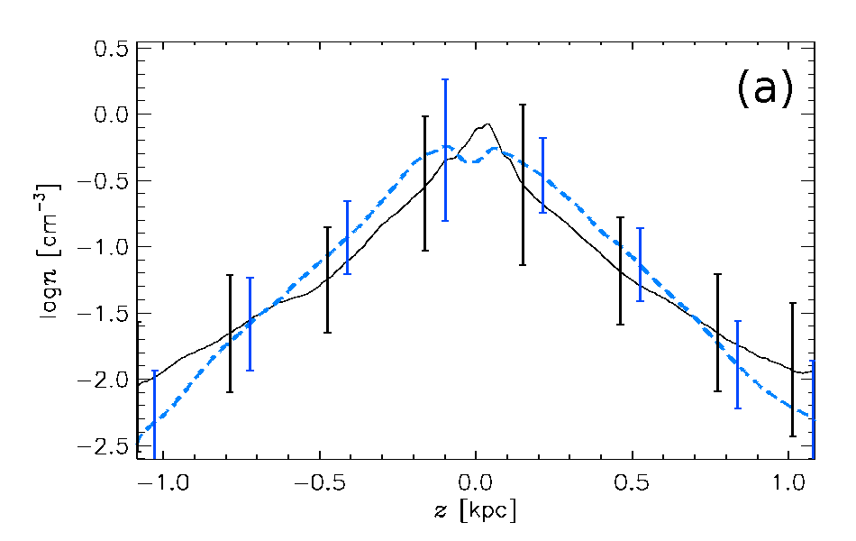
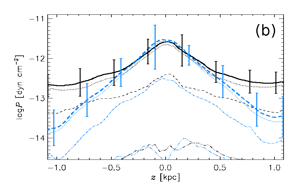
Figure 7.9: Horizontal averages of (a) gas number density, $\overline{n}(z)$, and (b) total pressure, $\overline{P}(z)$, for Model ${\mathrm{B}1\rm{\Omega}}^{*}$ (solid, black), and Model ${\mathrm{B}1\rm{\Omega}\rm{Sh}}$ (dashed, blue). Each is time-averaged using eleven snapshots spanning 600 to 700 Myr. The vertical lines indicate standard deviation within each horizontal slice. The thermal $\overline{p}(z)$ (dotted) and ram $\overline{p}_{\rm turb}(z)$ (fine dashed) pressures are also plotted (b). The magnetic pressure $\overline{p}_{B}$ is also plotted (fine, dash-3dotted).

The effect of increasing the shear (Model ${\mathrm{B}1\rm{\Omega}\rm{Sh}}$) can be seen from the comparisons with the results for Model ${\mathrm{B}1\rm{\Omega}}^{*}$, for the kinematic stage only. Temperatures are reduced, with ${\langle c{{}_{\mathrm{s}}}\rangle}\simeq 24\,{\rm km\,s^{-1}}$ against ${\langle c{{}_{\mathrm{s}}}\rangle}\simeq 58\,{\rm km\,s^{-1}}$, although in line with the other MHD models following the saturation of the dynamo, and also with ${\mathrm{B}1\rm{\Omega}\rm{SN}}$ for the kinematic stage only. However thermal energy ${\langle e_{\mathrm{th}}\rangle}\simeq 29E_{\mathrm{SN}}\,{\rm kpc}^{-3}$ is enhanced compared to Model ${\mathrm{B}1\rm{\Omega}}^{*}$. The velocities are almost half that of Model ${\mathrm{B}1\rm{\Omega}}^{*}$, with kinetic energy only slightly diminished, and matching that of Model ${\mathrm{B}1\rm{\Omega}\rm{SN}}$.

Otherwise shear appears to make little difference to the hydrodynamics. The probability distributions for the density, temperature, thermal and turbulent pressures are insensitive to the shear, except that the hot gas extends to significantly lower densities than for the other models. However, the shear does affect the vertical structure of the model, unlike the effect of increased rotation. In Fig. 7.9 the horizontal averages of density and pressure are plotted for Models ${\mathrm{B}1\rm{\Omega}}^{*}$ (black, taken from its kinematic period) and ${\mathrm{B}1\rm{\Omega}\rm{Sh}}$ (blue). The scale height of the density (panel a) is narrower for Model ${\mathrm{B}1\rm{\Omega}}^{*}$, with a higher density at the mid-plane. Given the twin peaks in the density profile for Model ${\mathrm{B}1\rm{\Omega}\rm{Sh}}$, the higher scale height appears to be an indirect effect of the magnetic field, rather than of the shear itself. As discussed in Chapter 9, the regular part of the magnetic field is strongest just outside of the SN active region, and can affect the location of the gas. This is evident in the twin peaks of the magnetic pressure (panel b, blue, dash-triple-dotted). The total pressure near the mid-plane is about the same for both models, but falls more rapidly away from the mid-plane for Model ${\mathrm{B}1\rm{\Omega}\rm{Sh}}$. So increased shear enhances the vertical pressure gradient. For Model ${\mathrm{B}1\rm{\Omega}\rm{Sh}}$ ${\langle|\nabla\times{{\mbox{\boldmath$u$}}}|\rangle}=342\,{\rm km\,s^{-1}}\,{\rm kpc}^{-1}$ and ${\langle|\nabla\cdot{{\mbox{\boldmath$u$}}}|\rangle}=188\,{\rm km\,s^{-1}}\,{\rm kpc}^{-1}$. Although the potential flow is similar to Model ${\mathrm{B}1\rm{\Omega}}$, and stronger than Model ${\mathrm{B}2\rm{\Omega}}$ after saturation of the dynamo, for Model ${\mathrm{B}1\rm{\Omega}}^{*}$ in the kinematic stage ${\langle|\nabla\times{{\mbox{\boldmath$u$}}}|\rangle}=737\,{\rm km\,s^{-1}}\,{\rm kpc}^{-1}$ and ${\langle|\nabla\cdot{{\mbox{\boldmath$u$}}}|\rangle}=295\,{\rm km\,s^{-1}}\,{\rm kpc}^{-1}$. So the magnitude of the flows and the ratio of rotational to irrotational flow (1.8) are smaller than for Model ${\mathrm{B}1\rm{\Omega}}^{*}$ (2.5).

Supernova Rate

The reduction in SN rate in Model ${\mathrm{B}1\rm{\Omega}\rm{SN}}$ predictably reduces the temperatures ${\langle c{{}_{\mathrm{s}}}\rangle}$ and the thermal energy ${\langle e_{\mathrm{th}}\rangle}$, but velocities and kinetic energy are similar to Model ${\mathrm{B}1\rm{\Omega}\rm{Sh}}$, also in the kinematic stage (see Table 4.2).

There is more cold gas than for the other models, and there is less very diffuse gas. Otherwise the distributions of gas density, temperature and pressure, and the multi-phase structure are not strongly affected.

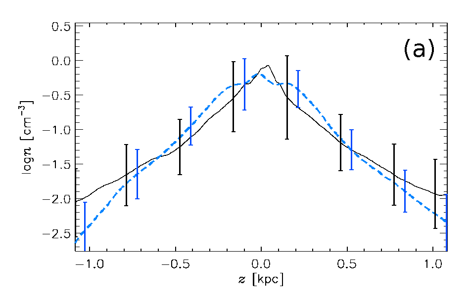
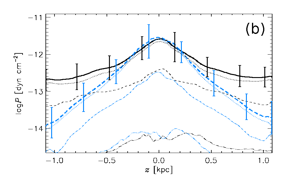
Figure 7.10: Horizontal averages of (a) gas number density, $\overline{n}(z)$, and (b) total pressure, $\overline{P}(z)$, for Model ${\mathrm{B}1\rm{\Omega}}^{*}$ (solid, black), and Model ${\mathrm{B}1\rm{\Omega}\rm{SN}}$ (dashed, blue). Each are time-averaged using eleven snapshots spanning 600 to 700 Myr. The vertical lines indicate standard deviation within each horizontal slice. The thermal $\overline{p}(z)$ (dotted) and ram $\overline{p}_{\rm turb}(z)$ (fine dashed) pressures are also plotted (b). The magnetic pressure $\overline{p}_{B}$ is also plotted (fine, dash-3dotted).

However the vertical distribution of the gas is affected by the SN rate. Similar to the increased shear, the reduced SN rate in Model ${\mathrm{B}1\rm{\Omega}\rm{SN}}$ increases the scale height of the gas density (Fig. 7.10a blue, dashed). Unlike Model ${\mathrm{B}1\rm{\Omega}\rm{SN}}$, there is a distinctive peak in density at the mid-plane. For Model ${\mathrm{B}1\rm{\Omega}\rm{SN}}$ ${\langle|\nabla\times{{\mbox{\boldmath$u$}}}|\rangle}=251\,{\rm km\,s^{-1}}\,{\rm kpc}^{-1}$ and ${\langle|\nabla\cdot{{\mbox{\boldmath$u$}}}|\rangle}=153\,{\rm km\,s^{-1}}\,{\rm kpc}^{-1}$. The potential flow is predictably reduced compared to Model ${\mathrm{B}1\rm{\Omega}}^{*}$, and also to Model ${\mathrm{B}1\rm{\Omega}\rm{Sh}}$. The ratio of rotational to irrotational flow is also reduced, at 1.6. The scale height of the gas density may be related to this ratio, given the similarities of Models ${\mathrm{B}1\rm{\Omega}\rm{SN}}$ and ${\mathrm{B}1\rm{\Omega}\rm{Sh}}$, with 1.6 and 1.8 respectively, and the similarities of Models ${\mathrm{B}1\rm{\Omega}}^{*}$ and ${\mathrm{B}2\rm{\Omega}}$, with 1.0 and 1.2 respectively. Alternatively there could be independent causes: the strong alignment of the magnetic field in the case of Model ${\mathrm{B}1\rm{\Omega}\rm{Sh}}$ and the reduced hot gas circulation induced by the SN forcing in Model ${\mathrm{B}1\rm{\Omega}\rm{SN}}$.

7.3 Summary

The cooling function affects the detail of the multi-phase structure, particularly the abundance of gas in the thermally unstable range, and the overall energy, because of differences in the cumulative cooling effect. However the separation into phases is not strongly sensitive to the form of the cooling function. Typical density, velocity and modal temperatures are quite consistent for each phase, independent of the cooling function. Supernova rate affects the thermodynamic properties, so reduced SNe produces cooler, less turbulent gas, given the same gas surface density. The perturbation and turbulent velocities, as well as the temperature are not sensitive to the rotation or shearing rate. However the relative vorticity of the system is affected by changes to any of these parameters.

Part IV Galactic magnetism: mean field and fluctuations

Chapter 8 Mean field in anisotropic turbulence

The ISM of spiral galaxies is extremely inhomogeneous, with SNe driving highly compressible, transonic turbulent motions, yet it supports magnetic fields at a global scale of a few kiloparsecs. Mean-field dynamo models have proven successful in modelling galactic magnetic fields, and offer a useful framework to study them and to interpret their observations (e.g., Beck et al., 1996; Shukurov, 2007). Turbulent dynamo action involves two distinct mechanisms. The fluctuation dynamo relies solely on the random nature of the fluid flow to produce random magnetic fields at scales smaller than the integral scale of the random motions. The mean-field dynamo produces magnetic field at a scale significantly larger than the integral scale, and requires rotation and stratification to do so. For any dynamo mechanism, it is important to distinguish the kinematic stage when magnetic field grows exponentially as it is too weak to affect fluid motions, and the nonlinear stage when the growth is saturated, and the system settles to a statistically steady state.

The scale of the mean field produced by the dynamo is controlled by the properties of the fluid flow. For example, in the simplest $\alpha^{2}$-dynamo in a homogeneous, infinite domain, the most rapidly growing mode of the mean magnetic field has scale of order $4\upi\eta_{\rm turb}/\alpha$, where $\alpha$ can be understood as the helical part of the random velocity and $\eta_{\rm turb}$ is the turbulent magnetic diffusivity (Sokoloff, Shukurov and Ruzmaikin, 1983). For any given $\alpha$ and $\eta_{\rm turb}$, this scale is finite and the mean field produced is, of course, not uniform.

In galaxies, the helical turbulent motions and differential rotation drive the so-called $\alpha\omega$-dynamo, where the mean field has a radial scale of order $\Delta r\simeq 3|{\cal{D}}|^{-1/3}(hR)^{1/2}$ at the kinematic stage (Starchenko and Shukurov, 1989), with ${\cal{D}}$ the dynamo number, $h\simeq 0.5\,{\rm kpc}$ the half-thickness of the dynamo-active layer and $R\simeq 3\,{\rm kpc}$ the scale of the radial variation of the local dynamo number. For $|{\cal{D}}|=20$, this yields $\Delta r\simeq 1.3\,{\rm kpc}$.

These estimates refer to the most rapidly growing mode of the mean magnetic field in the kinematic dynamo; it can be accompanied by higher modes that have a more complicated structure. Magnetic field in the saturated state can be even more inhomogeneous due to the local nature of dynamo saturation. The mean magnetic field can have a nontrivial, three-dimensional spatial structure, and any analysis of global magnetic structures must start with the separation of the mean and random (fluctuating) parts. However, many numerical studies of mean-field dynamos define the mean magnetic field as a uniform field obtained by averaging over the whole volume available; or in the case of fields showing non-trivial variations in a certain direction, as planar averages, e.g., over horizontal planes for systems that show $z$-dependent fields (e.g., Brandenburg and Subramanian, 2005).

The mean and random magnetic fields are assumed to be separated by a scale, $\lambda$, of order the integral scale of the random motions, $l_{\rm turb}$; $\lambda$ is not necessarily precisely equal to $l_{\rm turb}$, however, and must be determined separately for specific dynamo systems. The leading large-scale dynamo eigenmodes themselves have extended Fourier spectra, both at the kinematic stage and after distortions by the dynamo nonlinearity. Thus, both the mean and random magnetic fields are expected to have a broad range of scales, and their spectra can overlap in wavenumber space. It is therefore important to develop a procedure to isolate a mean magnetic field without unphysical constraints on its spectral content. This problem is especially demanding in the multi-phase ISM, where the extreme inhomogeneity of the system can complicate the spatial structure of the mean magnetic field.

The definition of the mean field as a horizontal average may be appropriate in some simplified numerical models, where the vertical component of the mean magnetic field, $\overline{B_{z}}$, vanishes because of periodic boundary conditions applied in $x$ and $y$; otherwise, $\nabla\cdot\overline{{{\mbox{\boldmath$B$}}}}=0$ cannot be ensured. An alternative averaging procedure that retains three-dimensional spatial structure within the averaged quantities is volume averaging with a kernel $G_{\ell}({{\mbox{\boldmath$r$}}}-{{\mbox{\boldmath$r^{\prime}$}}})$, where $\ell$ is the averaging length: ${\langle f({{\mbox{\boldmath$r$}}})\rangle}_{\ell}=\int_{V}f({{\mbox{\boldmath$r$}}}^{\prime})G_{\ell}({{\mbox{\boldmath$r$}}}-{{\mbox{\boldmath$r^{\prime}$}}})\,d^{3}{{\mbox{\boldmath$r$}}}^{\prime}$, for a scalar random field $f$.

Reynolds rules

A difficulty with kernel volume averaging, appreciated early in the development of turbulence theory, is that it does not obey the Reynolds rules of the mean (unless $\ell\to\infty$); i.e.

$${\langle{\langle f\rangle}_{\ell}g\rangle}_{\ell}\neq{\langle f\rangle}_{\ell}{\langle g\rangle}_{\ell}\qquad{\textrm{and}}\qquad{\langle{\langle f\rangle}_{\ell}\rangle}_{\ell}\neq{\langle f\rangle}_{\ell}$$ (8.1)

(Sect. 3.1 in Monin and Yaglom, 2007). If instead $\ell\to\infty$ and the mean is simply computed over the whole volume, then the total field can be decomposed into the mean and random parts, ${{\mbox{\boldmath$B$}}}={{\mbox{\boldmath$B$}}}_{0}+{{\mbox{\boldmath$b$}}}$, where ${{\mbox{\boldmath$B$}}}_{0}=\overline{{{\mbox{\boldmath$B$}}}}$ and $\overline{{{\mbox{\boldmath$b$}}}}={{\mbox{\boldmath$0$}}}$. The decomposition for the magnetic energies then follows conveniently as

$$\overline{{{\mbox{\boldmath$B$}}}^{2}}=\overline{({{\mbox{\boldmath$B$}}}_{0}+{{\mbox{\boldmath$b$}}})^{2}}=\overline{{{\mbox{\boldmath$B$}}}_{0}^{2}+2{{{{\mbox{\boldmath$B$}}}_{0}\cdot{{\mbox{\boldmath$b$}}}}}+{{\mbox{\boldmath$b$}}}^{2}}=\overline{{{\mbox{\boldmath$B$}}}}_{0}^{2}+\overline{{{\mbox{\boldmath$b$}}}^{2}}$$ (8.2)

Horizontal averaging represents a special case with $\ell\to\infty$ in two dimensions, or alternatively can be considered an average over the total ‘volume’ of each horizontal slice, and thus satisfies the Reynolds rules; however, the associated loss of a large part of the spatial structure of the mean field limits its usefulness. Kernel volume averaging retains the spatial structure, but critically ${\langle{{\mbox{\boldmath$b$}}}\rangle}_{\ell}$ in general does not equal $\mathrm{𝟎}$. The decomposition of the total magnetic energy ${{\mbox{\boldmath$B$}}}^{2}$ into mean and fluctuating energies cannot so conveniently be recovered from the quadratic terms ${\langle{{\mbox{\boldmath$B$}}}\rangle}_{\ell}^{2}$ and ${{\mbox{\boldmath$b$}}}^{2}$. An alternative formulation must be devised.

Germano approach to turbulence

Germano (1992) suggested a consistent approach to volume averaging which does not rely on the Reynolds rules. A clear, systematic discussion of these ideas is provided by Eyink (2012, Chapter 2), and an example of their application can be found in Eyink (2005). The averaged Navier–Stokes and induction equations remain unaltered, independent of the averaging used, if the mean Reynolds stresses and the mean electromotive force are defined in an appropriate, generalised way. The equations for the fluctuations naturally change, and care must be taken for their correct formulation. An important advantage of averaging with a Gaussian kernel (Gaussian smoothing) is its similarity to astronomical observations, where such smoothing arises from the finite width of a Gaussian beam, or is applied during data reduction.

In this chapter, I consider the magnetic field $B$ produced by the rotational shear and random motions in Model ${\mathrm{B}2\rm{\Omega}}$ with $\Omega=-S=2\Omega_{0}$. $\Omega_{0}=25\,{\rm km\,s^{-1}}\,{\rm kpc}^{-1}$ is the angular velocity in the Solar vicinity. This model has the fastest dynamo of all the magnetic runs in Table 4.1, so was adopted pragmatically to allow me to follow the dynamo process from early in the kinematic stage through to saturation and beyond. All of the magnetic models included in this thesis, however, appear to have produced a dynamo, so this analysis would be equally valid for all cases, were there sufficient resources to track them fully to the non-linear stage.

Using Gaussian smoothing, an approach is suggested, below, to determine the appropriate length $\ell$, and then obtain the mean magnetic field ${{\mbox{\boldmath$B$}}}_{\ell}$. The procedure ensures that $\nabla\cdot{{\mbox{\boldmath$B$}}}_{\ell}=0$. The random magnetic field $b$ is then obtained as ${{\mbox{\boldmath$b$}}}={{\mbox{\boldmath$B$}}}-{{\mbox{\boldmath$B$}}}_{\ell}$. The Fourier spectra of the mean and random magnetic fields overlap in wavenumber space, but their maxima are well separated.

8.1 The mean magnetic field

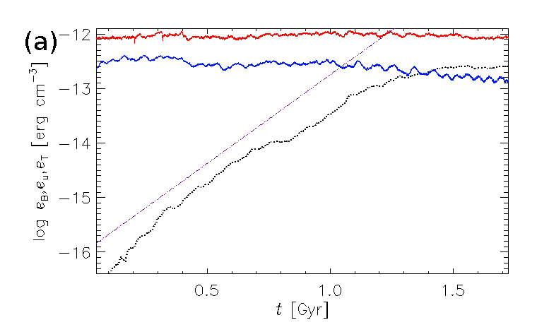
Figure 8.1: Evolution of energy densities averaged over the whole computational domain; thermal ${\langle e_{\mathrm{T}}\rangle}$ (red), kinetic ${\langle e_{\mathrm{u}}\rangle}$ (blue) and magnetic ${\langle e_{\mathrm{B}}\rangle}$ (black). Guide line (purple, dotted) indicates $\exp(7.5t\,{\rm Gyr}^{-1})$.

Figure 8.1 demonstrates the approximately exponential growth of magnetic energy density against the (relatively) stationary background of turbulent motions and thermal structure. As the average magnetic energy density ${\langle e_{\mathrm{B}}\rangle}={\langle|{{\mbox{\boldmath$B$}}}|^{2}\rangle}/8\upi$ becomes comparable to the average kinetic energy density ${\langle e_{\mathrm{u}}\rangle}$ at $t>1\,{\rm Gyr}$, the latter shows a modest reduction, as expected for the conversion of the kinetic energy of random motions to magnetic energy. The use of ${\langle\rangle}$ without subscript indicates averaging over the total numerical domain, analogous to the use of overbar in Eq. (8.2). For $t>1.4\,{\rm Gyr}$, the magnetic field settles to a statistically steady state with ${\langle e_{\mathrm{B}}\rangle}\approx 2.5\times 10^{-13}\,{\rm erg}\,{\rm cm}^{-3}$, somewhat larger than ${\langle e_{\mathrm{u}}\rangle}\approx 1.6\times 10^{-13}\,{\rm erg}\,{\rm cm}^{-3}$, while the thermal energy density ${\langle e_{\mathrm{T}}\rangle}\approx 10^{-12}\,{\rm erg}\,{\rm cm}^{-3}$ appears only weakly affected. Due to changes to the flow and thermodynamic composition, Ohmic heating is offset by reduced viscous heating or more efficient radiative cooling.

Magnetic field $B$ can be decomposed into ${{\mbox{\boldmath$B$}}}_{\ell}$, the part averaged over the length scale $\ell$, and the complementary fluctuations $b$,

$${{\mbox{\boldmath$B$}}}={{\mbox{\boldmath$B$}}}_{\ell}+{{\mbox{\boldmath$b$}}},\quad{{\mbox{\boldmath$B$}}}_{\ell}={\langle{{\mbox{\boldmath$B$}}}\rangle}_{\ell},\quad{{\mbox{\boldmath$b$}}}={{\mbox{\boldmath$B$}}}-{{\mbox{\boldmath$B$}}}_{\ell},$$ (8.3)

using volume averaging with a Gaussian kernel:

$${\langle{{\mbox{\boldmath$B$}}}\rangle}_{\ell}({{\mbox{\boldmath$x$}}}) =\int_{V}{{\mbox{\boldmath$B$}}}({{\mbox{\boldmath$x$}}}^{\prime})G_{\ell}({{\mbox{\boldmath$x$}}}-{{\mbox{\boldmath$x$}}}^{\prime})\,{\rm d}^{3}{{\mbox{\boldmath$x$}}}^{\prime},$$ (8.4)

$$G_{\ell}({{\mbox{\boldmath$x$}}}) =\left(2\upi\ell^{2}\right)^{-{3}/{2}}\exp\left[-{{{\mbox{\boldmath$x$}}}^{2}}/({2\,\ell^{2}})\right],$$

where $V$ is the volume of the computational domain. This operation preserves the solenoidality of both ${{\mbox{\boldmath$B$}}}_{\ell}$ and $b$, and retains their three-dimensional structure. For computational efficiency, the averaging was performed in the Fourier space where the convolution of Eq. (8.4) reduces to the product of Fourier transforms.

$${{\mbox{\boldmath$\hat{B}$}}}_{\ell}({{\mbox{\boldmath$k$}}},\ell)={{\mbox{\boldmath$\hat{B}$}}}({{\mbox{\boldmath$k$}}})\exp\left\{-2(\ell\upi)^{2}{{\mbox{\boldmath$k$}}}\cdot{{\mbox{\boldmath$k$}}}\right\}\,,$$

where ${{\mbox{\boldmath$\hat{B}$}}}({{\mbox{\boldmath$k$}}})={\cal{F}}\left[{{\mbox{\boldmath$B$}}}({{\mbox{\boldmath$x$}}})\right]$ and ${{\mbox{\boldmath$\hat{B}$}}}_{\ell}({{\mbox{\boldmath$k$}}},\ell)={\cal{F}}\left[{{\mbox{\boldmath${B}$}}}_{\ell}({{\mbox{\boldmath$x$}}},\ell)\right]$.

Since the averaging (8.4) does not obey the Reynolds rules for the mean, the definitions of various averaged quantities should be generalised as suggested by Germano (1992). In particular, the local energy density of the fluctuation field is given by

$$e_{b}({{\mbox{\boldmath$x$}}})=\frac{1}{8\upi}\int_{V}|{{\mbox{\boldmath$B$}}}({{\mbox{\boldmath$x$}}}^{\prime})-{{\mbox{\boldmath$B$}}}_{\ell}({{\mbox{\boldmath$x$}}})|^{2}G_{\ell}({{\mbox{\boldmath$x$}}}-{{\mbox{\boldmath$x$}}}^{\prime})\,{\rm d}^{3}{{\mbox{\boldmath$x$}}}^{\prime},$$ (8.5)

while

$${\langle e_{B}({{\mbox{\boldmath$x$}}})\rangle}_{\ell}= \frac{1}{8\upi}\int_{V}|{{\mbox{\boldmath$B$}}}({{\mbox{\boldmath$x$}}}^{\prime})|^{2}G_{\ell}({{\mbox{\boldmath$x$}}}-{{\mbox{\boldmath$x$}}}^{\prime}){\rm d}^{3}{{\mbox{\boldmath$x$}}}^{\prime}$$

$$e_{B\ell}({{\mbox{\boldmath$x$}}})= \frac{1}{8\upi}{|{{\mbox{\boldmath$B$}}}_{\ell}({{\mbox{\boldmath$x$}}})|^{2}}$$

This ensures that ${\langle e_{B}\rangle}_{\ell}=e_{B_{\ell}}+e_{b}$.

Expanding ${{\mbox{\boldmath$B$}}}({{\mbox{\boldmath$x$}}}^{\prime})$ in a Taylor series around $x$, and using

$$\int_{V}G_{\ell}({{\mbox{\boldmath$x$}}}-{{\mbox{\boldmath$x$}}}^{\prime})\,{\rm d}^{3}{{\mbox{\boldmath$x$}}}^{\prime}=1$$

(normalisation), and

$$\int_{V}({{\mbox{\boldmath$x$}}}-{{\mbox{\boldmath$x$}}}^{\prime})G_{\ell}({{\mbox{\boldmath$x$}}}-{{\mbox{\boldmath$x$}}}^{\prime})\,{\rm d}^{3}{{\mbox{\boldmath$x$}}}^{\prime}=0$$

(symmetry of the kernel), it can be shown that $e_{b}=|{{\mbox{\boldmath$b$}}}|^{2}/(8\upi)+O(\ell/L)^{2}$, where $L$ is the scale of the averaged magnetic field, defined as $L^{2}=|{{\mbox{\boldmath$B$}}}_{\ell}|/|\nabla^{2}{{\mbox{\boldmath$B$}}}_{\ell}|$ in terms of the characteristic magnitude of ${{\mbox{\boldmath$B$}}}_{\ell}$ and its second derivatives. Thus the difference between the ensemble and volume averages rapidly decreases as the averaging length decreases, $\ell/L\to 0$, or if the averaging is performed over the whole space, $L\to\infty$; this quantifies the deviations from the Reynolds rules for finite $\ell/L$.

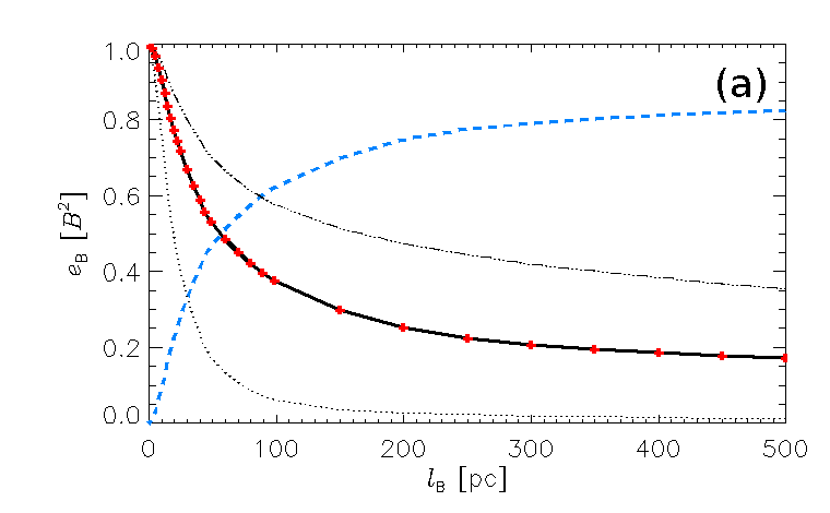
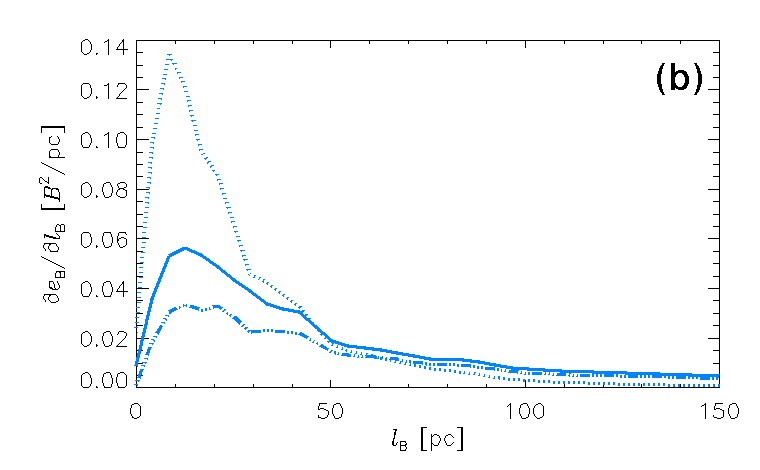
Figure 8.2: (a) Energy densities at $t=1.2\,{\rm Gyr}$ of mean, ${\langle e_{B_{\ell}}\rangle}$ (black, solid), and fluctuating, ${\langle e_{b}\rangle}$ (blue, dashed), magnetic fields as functions of the averaging length $\ell$, normalised by ${\langle{\langle e_{\mathrm{B}}\rangle}_{\ell}\rangle}$ and averaged over the region $|z|<0.5\,{\rm kpc}$; also ${\langle e_{B_{\ell}}\rangle}$ at $t=0.8\,{\rm Gyr}$ (dotted) and $t=1.6\,{\rm Gyr}$ (dash-triple-dotted). Values of $\ell$ sampled are indicated by red crosses. (b) Derivative of ${\langle e_{b}\rangle}$ from Panel (a) with respect to $\ell$, with the same line types.

The appropriate choice of $\ell$ is not obvious. The decomposition into ${{\mbox{\boldmath$B$}}}_{\ell}$ and $b$ was considered, through applying the averaging over a range $0<\ell<500\,{\rm pc}$ to 37 snapshots of the magnetic field between $t=0.8$ and 1.7 Gyr. The results for $t=0.8$, 1.2 and $1.6\,{\rm Gyr}$ are shown in Fig. 8.2. The smaller is $\ell$, the closer the correspondence between the averaged field and the original field (since the average is effectively sampling a smaller local volume), and hence the smaller the part of the total field considered as the fluctuation. Hence ${\langle B_{\ell}^{2}\rangle}$ is a monotonically decreasing function of $\ell$, whereas ${\langle b^{2}\rangle}$ monotonically increases (Fig. 8.2a). The curves for $t=0.8$ and 1.6 Gyr merely demonstrate that as the field grows over time, the mean field becomes more dominant. There is a corresponding shift downward with time of the curve for ${\langle e_{b}\rangle}$, so that the length $\ell_{B}$, where they are in equipartition, increases. A length scale defining the mean would not be expected to vary, at least in the kinematic stage.

It may be helpful to identify that value of $\ell$ where the variation of ${{\mbox{\boldmath$B$}}}_{\ell}$ and $b$ with $\ell$ becomes weak enough. To facilitate this, consider the rate of change of the relevant quantities with $\ell$, shown in Fig. 8.2b (note the different scale of the horizontal axis in this panel). The length $\ell\approx 50\,{\rm pc}$ is clearly distinguished: all the curves in Panel (b) are rather featureless for $\ell>50\,{\rm pc}$. The values in Fig. 8.2 have been obtained from the part of the domain with $|z|<0.5\,{\rm kpc}$, where most of the gas resides and where dynamo action is expected to be most intense. The results, however, remain quite similar if the whole computational domain $|z|\leq 1\,{\rm kpc}$ is used. While this value of $\ell$ has been estimated in a rather heuristic and approximate manner, the analysis of the magnetic power spectra in Section 8.2 confirms that $\ell=50\,{\rm pc}$ is close to the optimal choice.

To put the estimate $\ell\approx 50\,{\rm pc}$ into context, note that it is about half the integral scale of the random motions, $l_{\rm turb}$, estimated in Section 6.2. Simulations of a single SN remnant in an ambient density similar to that at $z=0$ (Appendix A.1) also show that the expansion speed of the remnant reduces to the ambient speed of sound when its radius is 50–70 pc.

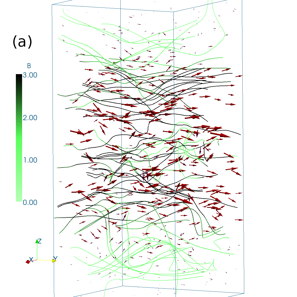
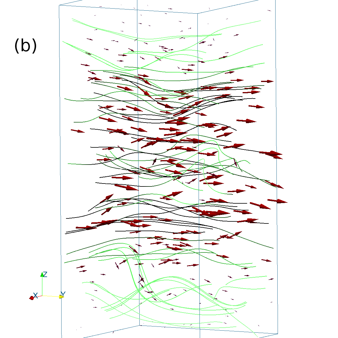
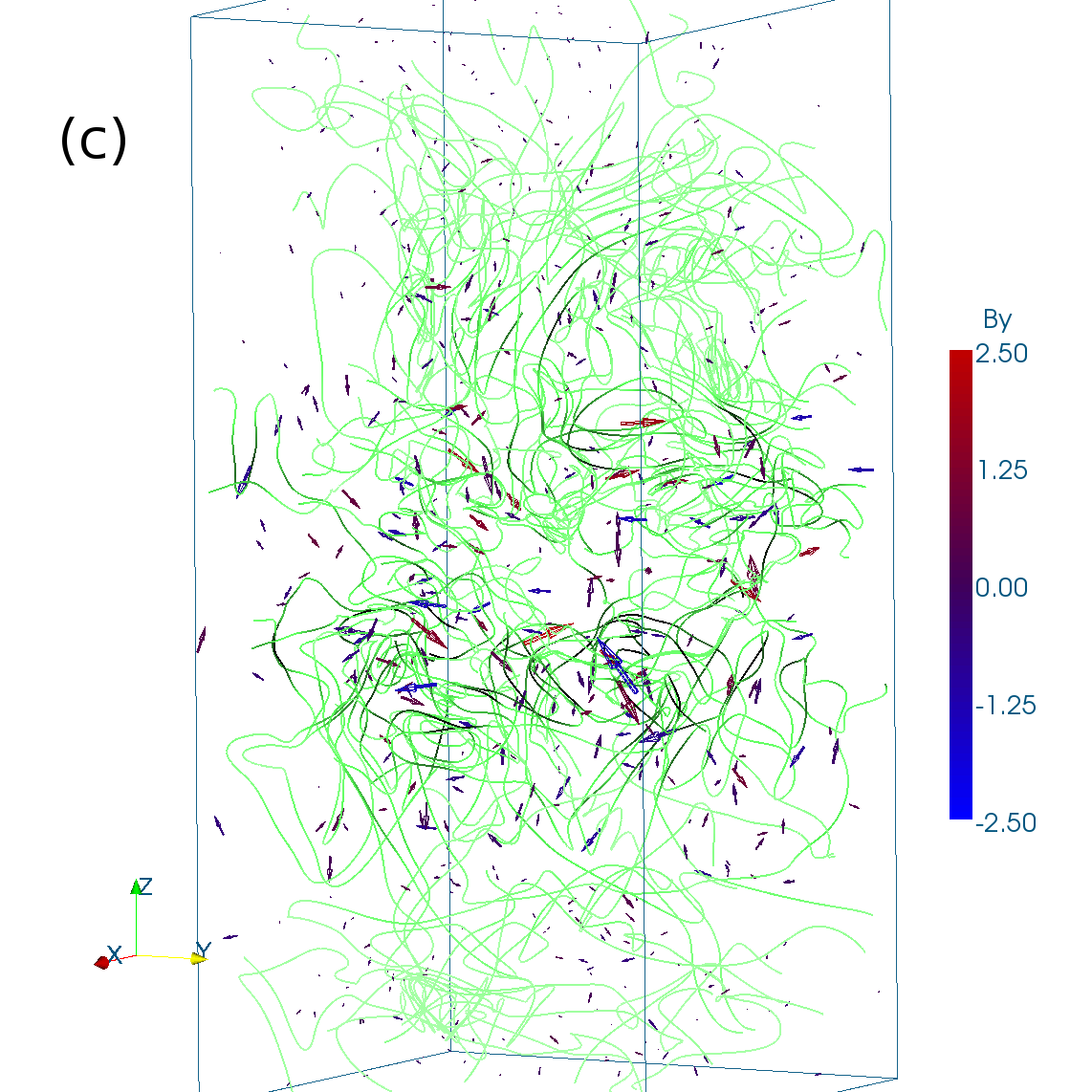
Figure 8.3: Field lines of (a) the total magnetic field $B$, (b) its averaged part ${{\mbox{\boldmath$B$}}}_{\ell}$, (c) the fluctuations $b$, obtained by averaging with $\ell=50\,{\rm pc}$, for $t=1.625\,{\rm Gyr}$. Field directions are indicated by arrows. The colour of the field lines indicates the field strength (colour bar on the left), whereas the vectors are coloured according to the strength of the azimuthal ($y$) component (colour bar on the right).

Figure 8.3 illustrates the total, mean and random magnetic fields thus obtained. For this saturated state, the field has a very strong uniform azimuthal component and a weaker radial component. The orientation of the field is the same above and below the mid-plane ($B_{y}>0$ and $B_{x}<0$), with maxima located at $|z|\approx 0.2\,{\rm kpc}$; the results will be reported in greater detail in Part V.

8.2 Scale separation

Scale separation between the mean and random magnetic fields in natural and simulated turbulent dynamos remains a controversial topic. The signature of scale separation sought for is a pronounced minimum in the magnetic power spectrum at an intermediate scale, larger than the energy-range scale of the random flow and smaller than the size of the computational domain. The power spectrum for $B$ is ${\color[rgb]{0,0,0}{M(k)=k^{-2}{{\langle|\mathcal{F}({k})|\rangle}_{k}},}}$ for spherical shells of thickness $\delta k$ at radius $k=|{{\mbox{\boldmath$k$}}}|$, from ${\color[rgb]{0,0,0}{\mathcal{F}({{\mbox{\boldmath$k$}}})={\int_{V}{{\mbox{\boldmath$B$}}}({{\mbox{\boldmath$x$}}})\exp({-2\pi i{{\mbox{\boldmath$k$}}}\cdot{{\mbox{\boldmath$x$}}}}){\rm d}^{3}{{\mbox{\boldmath$x$}}}}.}}$ The spectra of the mean and random magnetic fields obtained by Gaussian smoothing, shown in Fig. 8.4, have maxima at significantly different wavenumbers. Note however that the spectrum of the total magnetic field does not have any noticeable local minima and, with the standard approach (e.g., based on horizontal averages), the system would be considered to lack scale separation.

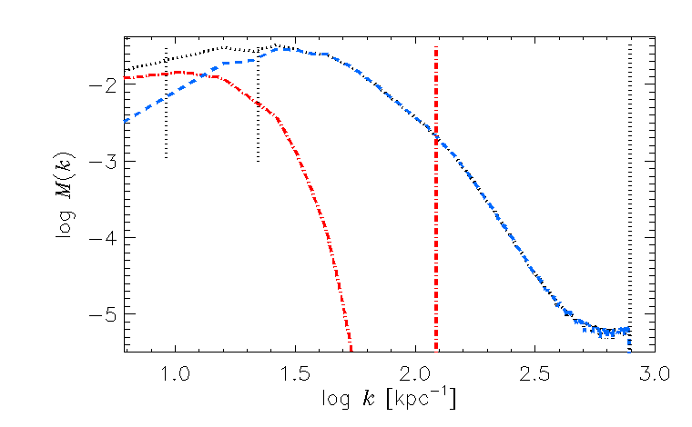
Figure 8.4: Power spectra of total (black, dotted), mean (red, dash-dotted) and fluctuating (blue, dashed) magnetic fields, for Gaussian smoothing with $\ell=50\,{\rm pc}$, at $t=1.05\,{\rm Gyr}$. Vertical red (dash-dotted) line marks the averaging wavenumber $2\upi\ell^{-1}$ and vertical black (dotted) line indicates the Nyquist wave number $\upi\Delta^{-1}$. Short vertical segments mark the energy-range scales $2\upi\mathcal{L}_{\ell}^{-1}$ and $2\upi\mathcal{L}_{b}^{-1}$ of the mean and random magnetic fields, respectively, obtained from Eq. (8.6).

figure 8.4 shows the magnetic power spectra of $B$, ${{\mbox{\boldmath$B$}}}_{\ell}$ and $b$. Note that $\ell$ is not located between the maxima in the power spectra of ${{\mbox{\boldmath$B$}}}_{\ell}$ and $b$; in fact, the spectral density of the mean field is negligible for $k\simeq 2\upi\ell^{-1}$. This can be understood from the transform of the kernel $G_{\ell}({{\mbox{\boldmath$x$}}})$, i.e. $\widehat{G}_{\ell}({{\mbox{\boldmath$k$}}})=\exp(-\ell^{2}{{\mbox{\boldmath$k$}}}^{2}/2)$; this kernel would divide a purely sinusoidal field equally into the mean and random parts at the wavelength $\lambda_{\rm eq}=\sqrt{2/\ln 2}\upi\ell$. For $\ell=50\,{\rm pc}$, $\lambda_{\rm eq}=0.27\,{\rm kpc}$, and the latter figure is a better guide to the expected separation scale. The separation of scales is immediately apparent in the spectra of the mean and random fields, $M_{\ell}(k)$ and $M_{b}(k)$, with the former having a broad absolute maximum at about $0.56\,{\rm kpc}$, and the latter a broad maximum near $0.2\,{\rm kpc}$. The effective separation scale $\lambda\approx 0.48\,{\rm kpc}$ can be identified where $M_{\ell}(k)=M_{b}(k)$, i.e. where the curves cross at $\log k\simeq 1.1$.

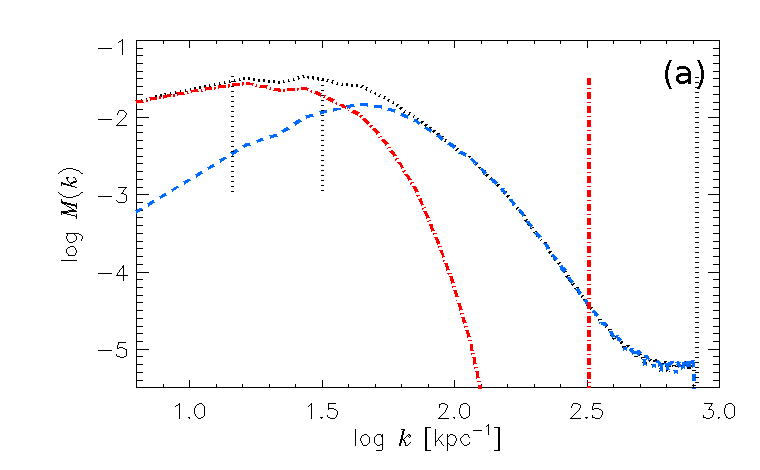
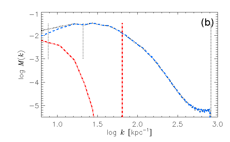
Figure 8.5: As Fig. 8.4, but for (a) $\ell=20\,{\rm pc}$ and (b) $\ell=100\,{\rm pc}$.

The integral scales of ${{\mbox{\boldmath$B$}}}_{\ell}$ and $b$ can be obtained from their spectral densities as

$$\mathcal{L}_{\ell}=\frac{\upi}{2}\,{\int_{{2\upi}/{D}}^{{\upi}/{\Delta}}k^{-1}M(k)\,{\rm d}k}\left[{\int_{{2\upi}/{D}}^{{\upi}/{\Delta}}M(k)\,{\rm d}k}\right]^{-1},$$ (8.6)

where $\Delta$ is the numerical grid separation and $D$ is the size of the domain (Section 12.1, Monin and Yaglom, 2007). This yields $\mathcal{L}_{\ell}\simeq 0.67\,{\rm kpc}$ and $\mathcal{L}_{b}\simeq 0.28\,{\rm kpc}$ for ${{\mbox{\boldmath$B$}}}_{\ell}$ and $b$, respectively (Fig. 8.4).

As the magnetic field strength grows, the magnitudes of the spectral densities change but the characteristic wavenumbers vary rather weakly. $\mathcal{L}_{\ell}$ remains close to $0.7\,{\rm kpc}$ throughout the kinematic phase, increasing only beyond 1.1 Gyr to about $0.9\,{\rm kpc}$. $\mathcal{L}_{b}$ increases from $0.23$ to $0.28\,{\rm kpc}$ during the kinematic phase, but rises to $0.4\,{\rm kpc}$ after the system saturates. The stability of $\mathcal{L}_{\ell}$ is consistent with the eigenmode amplification of the mean magnetic field as expected for a kinematic dynamo, and supports $\ell\approx 50\,{\rm pc}$ as a reasonable choice of the averaging scale.

Figure 8.5 presents magnetic energy spectra obtained using $\ell=20\,{\rm pc}$ and $100\,{\rm pc}$. In the former, the effective separation scale $\lambda\approx 0.16\,{\rm kpc}$ is less than $\mathcal{L}_{b}\simeq 0.21\,{\rm kpc}$. This is inconsistent, implying that energy at scales about $\mathcal{L}_{b}$ lies predominantly within ${{\mbox{\boldmath$B$}}}_{\ell}$. For $\ell=100\,{\rm pc}$, $\lambda\geq 1\,{\rm kpc}$ is greater than $\mathcal{L}_{\ell}\simeq 0.81\,{\rm kpc}$, which is also inconsistent. Significantly, applying $\ell=50\,{\rm pc}$ satisfies $\mathcal{L}_{b}<\lambda<\mathcal{L}_{\ell}$. Hence the scale $\lambda$, at which the dominant energy contribution switches between the mean and fluctuating parts, is here consistent only with $\ell\simeq 50\,{\rm pc}$.

As well as different spatial scales, the mean and random magnetic field energies have different exponential growth rates (Fig. 8.6), given in Table 8.1. The growth for the mean field component of the total magnetic energy is denoted by $\Gamma_{e}$ and the growth of the random field energy by $\gamma_{e}$. Results from horizontal averaging are also given; they differ from those obtained with Gaussian smoothing, especially for the mean field. The growth rate $\Gamma_{e}$ of the mean-field energy is controlled by the shear rate, mean helicity of the random flow, and the turbulent magnetic diffusivity. Any mean magnetic field is accompanied by a random field, which is part of the mean-field dynamo mechanism (as any large-scale magnetic field is tangled by the random flow); the energy of this part of the small-scale field should grow at the same rate $\Gamma_{e}$ as the mean energy. The fluctuation dynamo produces another part of the random field whose energy growth rate depends on the turbulent kinematic time scale $l/u$, and the magnetic Reynolds and Mach numbers. The difference between $\Gamma_{e}$ and $\gamma_{e}$ obtained suggests that both mean-field and fluctuation dynamos are present in our model. The growth rate of the mean magnetic energy is roughly double that of the random field for both types of averaging. This is opposite to what is usually expected, plausibly because of the inhibition of the fluctuation dynamo by the strongly compressible nature of the flow and low Reynolds numbers available at this resolution. We would expect the fluctuation dynamo to be stronger with more realistic Reynolds numbers.

Table 8.1: Exponential growth rates of energy in the mean and random magnetic fields, $\Gamma_{e}$ and $\gamma_{e}$, respectively, with associated values of reduced $\chi^{2}$. From exponential fits to the corresponding curves in Fig. 8.6, for $0.8<t<1.05\,{\rm Gyr}$. (Growth for $t<0.8\,{\rm Gyr}$ is similar to this interval – see Fig. 8.1.)

	$\Gamma_{e}$	$\chi^{2}$	$\gamma_{e}$	$\chi^{2}$
	[Gyr-1]		[Gyr-1]
Gaussian smoothing	$10.9$	$1.00$	5.5	$1.15$
Horizontal averaging	$13.6$	$0.25$	$6.2$	$0.25$

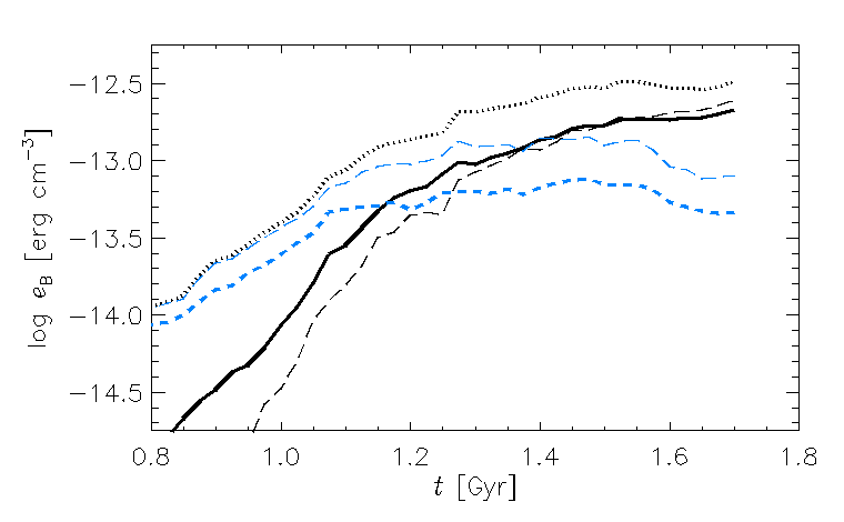
Figure 8.6: Evolution of magnetic energy densities, averaged for full domain: total magnetic field (black, dotted), mean (black, solid), and random (blue, dashed) obtained from Gaussian smoothing with $\ell=50\,{\rm pc}$. Energy densities of mean and random magnetic fields obtained from horizontal averaging are shown long-dashed (black and blue, respectively).

8.3 Evaluation of the method

The approach used here to identify the appropriate averaging length $\ell$ (and thus the effective separation scale $\lambda$) is simple (but not oversimplified); $\ell$ can in fact depend on position, and it may remain constant in time only at the kinematic stage of all the dynamo effects involved. Wavelet filtering may prove to be more efficient than Gaussian smoothing in assessing the variations of $\ell$.

At the kinematic stage, the spectral maximum of the mean field is already close to the size of the computational domain, and it cannot be excluded that the latter is too small to accommodate the most rapidly growing dynamo mode. These results should therefore be considered as preliminary with respect to the mean field; simulations in a bigger domain are clearly needed.

The physically motivated averaging procedure used here, producing a mean field with three-dimensional structure, may facilitate fruitful comparison of numerical simulations with theory and observations. Although Gaussian smoothing does not obey all the Reynolds rules, it is possible that a consistent mean-field theory can be developed, e.g. in the framework of the $\tau$-approximation (see e.g. Brandenburg and Subramanian, 2005, and references therein). This approach does not rely upon solving the equations for the fluctuating fields, and hence only requires the linearity of the average and its commutation with the derivatives. The properly isolated mean field is likely to exhibit different spatial and temporal behaviour than the lower-dimensional magnetic field obtained by two-dimensional averaging.

Brandenburg and Subramanian (2005, Ch.11.5) include estimates for the strength of the mean field dynamo in rapidly rotating galaxies. Here I apply their method to Model ${{\mathrm{B}2\rm{\Omega}}}$, to compare their estimates with the simulation results. The turnover time is given by $\tau=l_{\rm turb}/u_{\rm turb}$. From Section 6.2, $l_{\rm turb}\simeq 0.1\,{\rm kpc}$. The estimates assume incompressibility, so I shall use the upper bound of the subsonic turbulence. The mean field dynamo grows primarily in the warm gas, as is detailed in Part V. From Fig. 5.11, the modal temperature of the warm gas is $10^{4}\,{\rm K}$, which equates to $c{{}_{\mathrm{s}}}\simeq 15\,{\rm km\,s^{-1}}$, the upper bound for $u_{\rm turb}$. Hence $\tau\simeq 1/150\,{\rm Gyr}$.

The turbulent resistivity is $\eta_{\rm turb}={\textstyle{\frac{1}{3}}}u_{\rm turb}l_{\rm turb}\simeq 0.5\,{\rm km\,s^{-1}}\,{\rm kpc}$. From Fig. 9.2 in Part V, it is apparent that the scale height of the dynamo active region may be as high as $h\simeq 0.6\,{\rm kpc}$. So $\alpha=\tau^{2}\Omega(u_{\rm turb}^{2}/h)\simeq 5/6\,{\rm km\,s^{-1}}$. The $\alpha\Omega$-dynamo has two control parameters: $C_{\Omega}=Sh^{2}/\eta_{\rm turb}\simeq-36$ and $C_{\alpha}=\alpha h/\eta_{\rm turb}\simeq 1$, so the dynamo number $D=C_{\Omega}C_{\alpha}\simeq-36$.

If $|D|>D_{\mathrm{crit}}$, a critical dynamo number which the authors expect to be in the range $6$–$10$, then exponential growth of the magnetic field is possible during the kinematic stage. The growth rate exponent $\Gamma$ can be estimated by

$$\Gamma\approx\frac{\eta_{\rm turb}}{h^{2}}\left(\sqrt{|D|}-\sqrt{D_{\textrm{c}rit}}\right)$$ (8.7)

So for Model ${\mathrm{B}2\rm{\Omega}}$, the expected growth rate of the magnetic field $\Gamma$ is of order 4–5$\,{\rm Gyr}^{-1}$.

Note the growth rates $\Gamma_{e}$ shown in Table 8.1 refer to the magnetic energy, so $\Gamma_{e}=2\Gamma$ as estimated here. For Gaussian smoothing $\Gamma_{e}=10.9\,{\rm Gyr}^{-1}$, while for horizontal averaging it is $13.6\,{\rm Gyr}^{-1}$. Although the analytic estimates apply to incompressible flow and there is considerable uncertainty over the choices of $l_{\rm turb},~{}u_{\rm turb},~{}h$ and $D_{\textrm{crit}}$, a reasonable upper bound for this model is $\Gamma=6\,{\rm Gyr}^{-1}$. In addition, given the complexity of the system, other mean field dynamo processes could be present in addition to the shear dynamo to which the analytics refer. Nevertheless, the agreement of theory and experiment is very encouraging.

8.4 Summary

Using kernel smoothing to identify the mean field permits separation of the fluctuations from the systematic part of the magnetic field, while preserving its basic structure. The departure from the Reynolds rules is addressed by redefining how the magnetic energy terms are derived. A heuristic approach has been adopted to determine the appropriate smoothing scale, which appears to correctly identify the separation between the mean and random parts of the field. This allows us to examine the growth of the mean and random field, and a mean field dynamo has been modelled, with growth consistent with the analytic estimates for the galactic shear dynamo. In the remainder of this thesis, the method described in this chapter is applied to determine the mean $B$ field and the mean flow $u$ whenever they are required.

Part V The galactic dynamo and magnetic structure

Chapter 9 The magnetic field

In this chapter the magnetic field generated dynamically in the various MHD models is investigated in some detail. All the models in this section show sustained amplification of the magnetic field, and evident organisation into a mean field. Of interest to theorists is what is driving the dynamo, and where the dynamo or dynamos are acting. Of general interest is the general shape and structure of the magnetic field, to what extent is it ordered or fluctuating, and how strongly correlated is it to the density or temperature in the ISM. The vertical magnetic structure of the ISM is particularly difficult to observe, so how the simulated field varies with distance from the mid-plane is of great interest. How does the magnetic field interact with the velocity field, and to what extent are the properties of the ISM, such as distributions of temperature, pressure and density, or various filling factors, affected by the magnetic field? These issues will be considered by comparing the MHD models with each other and with the non-magnetic models.

9.1 The magnetic dynamo

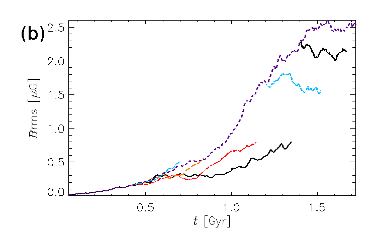
Figure 9.1: (a) Time evolution for the log of thermal (red, top jagged), kinetic (blue, $2^{\rm nd}$ top jagged) and magnetic (black, dotted) energy densities from Model ${\mathrm{B}2\rm{\Omega}}$, averaged over the total volume. The dotted line indicates $6.6\,{\rm Gyr}^{-1}$. (b) ${\langle B{{}_{\rm rms}}\rangle}$ as a function of time for Models ${\mathrm{B}1\rm{\Omega}}$ (solid, black), ${\mathrm{B}2\rm{\Omega}}$ (dashed, purple), ${\mathrm{B}1\rm{\Omega}\rm{O}}$ (dash-dotted, blue), ${\mathrm{B}1\rm{\Omega}\rm{Sh}}$ (long dashed, orange), and ${\mathrm{B}1\rm{\Omega}\rm{SN}}$ (dash-3dotted, red). The later continuations of Models ${\mathrm{B}1\rm{\Omega}}$ from 1.4 Gyr and ${\mathrm{B}1\rm{\Omega}\rm{O}}$ from 1.2 Gyr are Model ${\mathrm{B}2\rm{\Omega}}$ continued with parameters amended.

In Fig. 9.1a the time evolution of magnetic (purple), kinetic (blue) and thermal (red) log energy density is plotted for Model ${\mathrm{B}2\rm{\Omega}}$. The growth in kinetic energy density from rest, and thermal energy due to SN heating, is near instantaneous. The growth in ${\langle B{{}_{\rm rms}}\rangle}$ is much slower and irregular, intermittently exponential, linear and even occasionally exhibiting decay. Dynamo theory anticipates that, as magnetic energy density ($\,{e_{\rm B}}=\frac{1}{2\mu_{0}}|{{\mbox{\boldmath$B$}}}|^{2}$) approaches that of the kinetic energy density ($\,{e_{\rm kin}}=\frac{1}{2}\rho|{{\mbox{\boldmath$u$}}}|^{2}$), the magnetic field saturates to a steady state, with kinetic and magnetic energy near equipartition. The Lorentz Force feeds back onto the velocity field suppressing the kinematic dynamo. In Fig. 9.1a ${\langle\,{e_{\rm B}}\rangle}$ and ${\langle\,{e_{\rm kin}}\rangle}$ intersect at about 1.3 Gyr corresponding to ${\langle B{{}_{\rm rms}}\rangle}\simeq 2.5\,\umu{\rm G}$. This is remarkably consistent with the observed estimates of the field strength in the solar neighbourhood.

The thermal energy density ($\,{e_{\rm th}}=\rho\,{c_{\rm v}}T$), with $\,{c_{\rm v}}$ the specific heat capacity at constant volume) is quite insensitive to ${\langle\,{e_{\rm B}}\rangle}$, as is ${\langle\,{e_{\rm kin}}\rangle}$ up to 1 Gyr, with ${\langle\,{e_{\rm th}}\rangle}\simeq 9\times 10^{-13}$ and ${\langle\,{e_{\rm kin}}\rangle}\simeq 3\times 10^{-13}\,{\rm erg}\,{\rm cm^{-3}}$. However around 1.1 Gyr, when ${\langle\,{e_{\rm B}}\rangle}$ grows to within half of ${\langle\,{e_{\rm kin}}\rangle}$, kinetic energy is transferred to magnetic energy. There is also a slight reduction in ${\langle\,{e_{\rm th}}\rangle}$ after 1.4 Gyr, such that total energy density is roughly conserved, with ${\langle\,{e_{\rm B}}\rangle}\simeq 2.5\times 10^{-13}$, ${\langle\,{e_{\rm kin}}\rangle}\simeq 1.5\times 10^{-13}$ and ${\langle\,{e_{\rm th}}\rangle}\simeq 8\times 10^{-13}\,{\rm erg}\,{\rm cm^{-3}}$.

In Fig. 9.1b the time evolution of ${\langle B{{}_{\rm rms}}\rangle}$ is plotted for the MHD models. It is evident that all the models exhibit periods of exponential growth. At 400 Myr ${\mathrm{B}1\rm{\Omega}}$ is in quasi-steady hydrodynamic turbulence with negligible magnetic energy and the other models are initialised using this snapshot. Subsequently the lowest growth rate appears to apply for ${\mathrm{B}1\rm{\Omega}}$. However ${\mathrm{B}1\rm{\Omega}\rm{O}}$, plotted in blue dash-dotted in Fig. 9.1a, differs only in the open vertical boundary condition, and appears to attain stronger growth. For this model the Poynting flux is monitored on the boundary and the net outflow of magnetic energy throughout this phase is consistently of order $10^{2}$ times the inflow or greater. The growth would appear therefore to be driven by the internal dynamics, and potentially assisted by the flux of magnetic helicity outward.

In their models matching these parameters, Gressel et al. (2008a) found no dynamo. Only with differential galactic rotation $\geq 4\Omega_{0}$ did they observe a mean field dynamo. They resolved a grid of $\Delta=8\,{\rm pc}$, while here $\Delta=4\,{\rm pc}$, and I also use temperature dependent viscosity and thermal conductivity, which permit much larger Reynolds numbers. Consistent with their results, however, I do find the strongest dynamo corresponds to the higher rotation rate (plotted in purple, dashed in Fig. 9.1a).

Increasing the shear alone in Model ${\mathrm{B}1\rm{\Omega}\rm{Sh}}$ (plotted in orange, long dashes) also enhances magnetic field growth relative to Model ${\mathrm{B}1\rm{\Omega}}$. For spiral galaxies, which often have nearly flat rotation curves with respect to the galactocentric radius $r$, with angular velocity of the form $\Omega\propto r^{-1}$, the shear parameter $S=-\Omega$. It is convenient to introduce the ratio of the shear rate to the rotation rate:

$$q=-\frac{S}{\Omega}=-\frac{{\rm d}\ln\Omega}{{\rm d}\ln r}.$$ (9.1)

Flat rotation curves correspond to $q=1$. Such rotation laws are known to be hydrodynamically stable, as the Rayleigh instability only sets in for $q>2$. To exclude additional Rayleigh instability effects $-S/\Omega<2$ is required, so $S=-40\,{\rm km\,s^{-1}}\,{\rm kpc}^{-1}=-1.6\Omega_{0}$ is adopted, yielding $q=1.6$. There may however remain a contribution of magnetorotational instability (MRI), which has an instability condition of $q>0$. There is evidence, however, that this effect is suppressed in the presence of SN turbulence (Korpi, Käpylä and Väisälä, 2010; Piontek and Ostriker, 2007; Balbus and Hawley, 1991). Future work, comparing a model in which the sign of $S$ or $\Omega$ is reversed (so that $q<0$) to a standard model, may help to isolate the influence of MRI from the shear dynamo. Such a run, with the outer disc modelled to rotate faster than the inner disc, would not be relevent for any known galaxies, but other than a sign change in the mean horizontal components of the flow and the mean magnetic field, the ISM temperature, density and pressure distributions should be retained. The turbulent structure should be unaffected, at least in the kinematic stage.

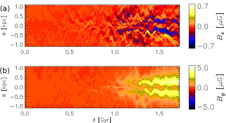
Figure 9.2: Time evolution of the horizontal averages for (a) $B_{x}$ and (b) $B_{y}$ for Model ${\mathrm{B}2\rm{\Omega}}$, with galactic rotation twice $\Omega_{0}$ and parameters otherwise typical of the Galaxy in the solar neighbourhood. The maximum strength of the seed field is $B_{y}<0.01\,\umu{\rm G}$.

In Fig. 9.2 the time evolution of $B_{x}$ and $B_{y}$, averaged horizontally, are plotted against $z$ for Model ${\mathrm{B}2\rm{\Omega}}$. Horizontally averaged $B_{z}\simeq 0$ for all $z$, although the random fluctuations are typically stronger than for $B_{x}$ and $B_{y}$. It is evident that a strong mean field is generated, that it is dominated by the azimuthal ($y$) component, and that the magnitudes of both $B_{y}$ and $B_{x}$ vary with $z$ and are roughly symmetric about the mid-plane.

That ${\langle B_{z}\rangle}\simeq 0$ is not a physical result, but imposed by the periodic and sliding periodic boundary conditions applied horizontally to all three components of the magnetic potential. Given the divergence free condition on the magnetic field in the galaxy, it is reasonable to expect that the mean radial field, which is oriented inwards on both sides of the mid-plane throughout the simulation, cannot meet at the centre of the galaxy. Towards the centre of the galaxy, there must be a significant mean vertical component. Of course for small galactic radius, the shearing box approximation breaks down anyway. Nevertheless in future work horizontal boundary conditions, which permit the free movement of the field lines, may reveal non trivial vertical field structure.

Reducing the supernova rate by 20% with Model ${\mathrm{B}1\rm{\Omega}\rm{SN}}$ (plotted in red, dash-dotted) also drives a stronger dynamo than ${\mathrm{B}1\rm{\Omega}}$. As discussed in Section 7.1, the investigation by Balsara et al. (2004) with SN rates of 8$\sigma_{0}$ to 40$\sigma_{0}$ indicates that as SN rates exceed some critical level, the amplification of the small scale field is quenched. The critical rate will be at least above $12\sigma_{0}$, based on their periodic box calculations, and will likely be higher, given the release of hot gas away from the mid-plane in the stratified ISM. It may also be reasonable to expect a minimum SN rate, below which the dynamo cannot operate. Gressel (2008) also found that the strength of the magnetic field increased for lower SN rates over a range from $0.25\sigma_{0}$ to $\sigma_{0}$.

The strongest ordered field corresponds to the layers between 200 and 600 pc away from the mid-plane in Fig. 9.2. Although the ordering of the field is stronger in Model ${\mathrm{B}2\rm{\Omega}}$, all the MHD models share this structure. The weaker mean field near the mid-plane may be a result of the scrambling of the field lines by SN turbulence. The strongest mean field occurs where the filling factors of the warm gas are highest, and outside the most active SN layer. This is consistent with the loss of field amplification as SN rates increase.

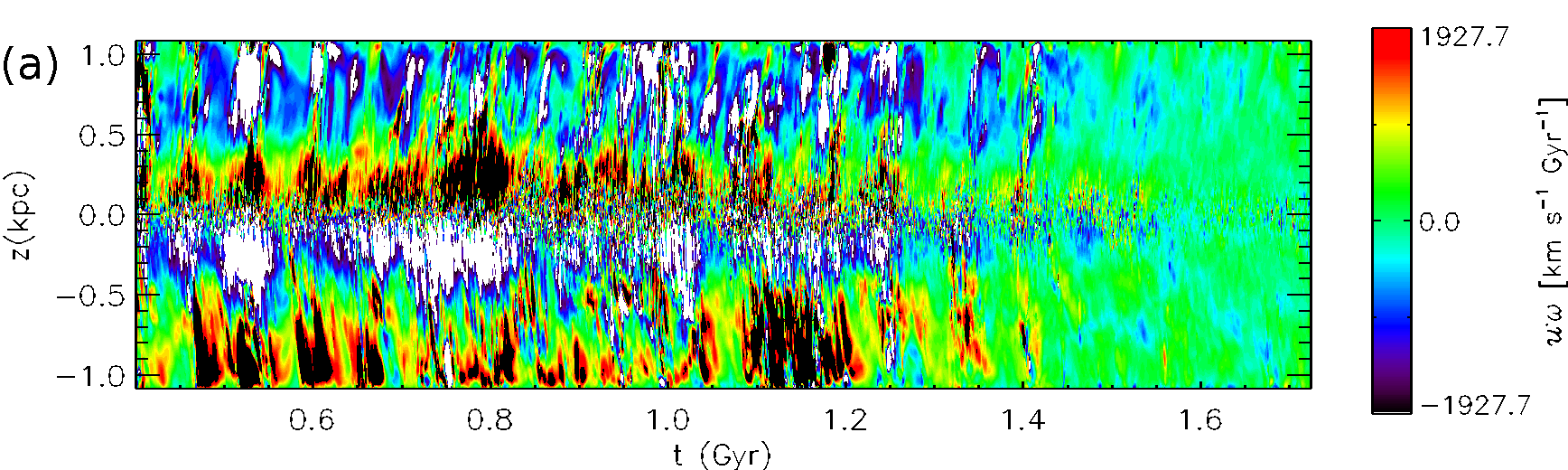
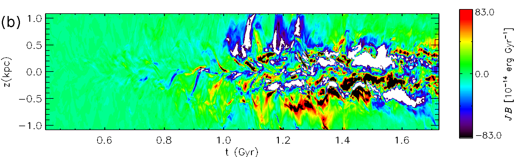
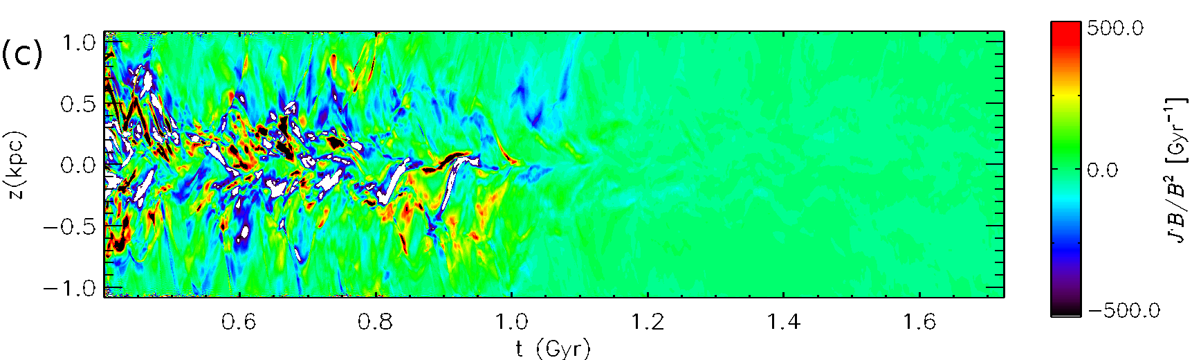
Figure 9.3: Time evolution from Model ${\mathrm{B}2\rm{\Omega}}$ of horizontal averages for (a) kinetic helicity (${{\mbox{\boldmath$u$}}}\cdot{{\mbox{\boldmath$\omega$}}}$), and (b) the current helicity ${{\mbox{\boldmath$J$}}}\cdot{{\mbox{\boldmath$B$}}}$, a gauge invariant proxy for magnetic helicity. In (c) the relative current helicity ${{\mbox{\boldmath$J$}}}\cdot{{\mbox{\boldmath$B$}}}$ normalised by ${\langle B{{}_{\rm rms}}^{2}\rangle}(t)$ is displayed. Regions of black (white) indicate values above (below) the colour bar range.

To understand what is driving the dynamo, it may help to look at the kinetic and magnetic helicity. The growth of magnetic helicity may suppress the dynamo. In Fig. 9.3, horizontal averages from Model ${\mathrm{B}2\rm{\Omega}}$ as a function of $z$ and evolving in time are displayed for (panel a) kinetic helicity (${{\mbox{\boldmath$u$}}}\cdot{{\mbox{\boldmath$\omega$}}}$) and (panel b) current helicity ${{\mbox{\boldmath$J$}}}\cdot{{\mbox{\boldmath$B$}}}$, a proxy for the magnetic helicity (${{\mbox{\boldmath$A$}}}\cdot{{\mbox{\boldmath$B$}}}$), but gauge invariant. ${{\mbox{\boldmath$J$}}}=\frac{c}{4\upi}\nabla\times{{\mbox{\boldmath$B$}}}$ in the time independent electric field. Hence, ${{\mbox{\boldmath$J$}}}\sim\mathcal{L}^{-2}{{\mbox{\boldmath$A$}}}$, where $\mathcal{L}$ is some integral scale of the magnetic potential, can be used to indicate the evolving structure without the requirement to deduct the contribution of the arbitrary gauge $\nabla\Phi$ from $A$. Fig. 9.3c shows ${{\mbox{\boldmath$J$}}}\cdot{{\mbox{\boldmath$B$}}}$, normalised by the time dependent ${\langle B{{}_{\rm rms}}^{2}\rangle}$, the relative current helicity, of use for comparing the kinematic stage with the saturated state.

From the first two plots it appears that the saturation of the dynamo beyond $1\,{\rm Gyr}$ coincides with the transfer of mean helicity from kinetic to magnetic form. This transfer is present in the saturated stages for Models ${\mathrm{B}1\rm{\Omega}}$ and ${\mathrm{B}1\rm{\Omega}\rm{O}}$ also. In (a), the kinetic helicity either side of the mid-plane is of opposite sign, negative in the south and positive in the north, as would be expected. What is surprising is that there is another sign change at $|z|\simeq 0.3\sim 0.5\,{\rm kpc}$. The pattern is most clearly revealed for Model ${\mathrm{B}2\rm{\Omega}}$, but is common to all of the MHD models and is also a consistent feature of the HD models. In the saturated stage the magnetic helicity appears to exhibit strong mean structures, and there is some tendency for sign asymmetry about the mid-plane, although this is fragmented. The sign of ${\langle B_{y}\rangle}$ is quite consistently positive in the latter stages, so the intermittent reversals in helicity are primarily due to the fluctuations in ${\langle B_{x}\rangle}$.

The stronger current helicity at later times, however, is primarily only a weak effect of a much stronger field. In Fig. 9.3c, where the normalised ${{\mbox{\boldmath$J$}}}\cdot{{\mbox{\boldmath$B$}}}$ is plotted, it is evident that the peak relative helicity occurs prior to field saturation up to $1.1\,{\rm Gyr}$. Throughout the simulation the net ${{\mbox{\boldmath$J$}}}\cdot{{\mbox{\boldmath$B$}}}$ is negative. The normalised $\overline{{\langle{{\mbox{\boldmath$J$}}}\cdot{{\mbox{\boldmath$B$}}}/{\langle B^{2}\rangle}\rangle}}=-6.0\,{\rm Gyr}^{-1}$ before saturation, where ${\langle\rangle}$ indicates averaging over the whole volume and the over-bar here refers to averaging over time, $0.4<t<1.1\,{\rm Gyr}$, and $-0.6\,{\rm Gyr}^{-1}$ post-saturation. Further details of this quantity are given in Table 9.1 for all the MHD models.

Table 9.1: For each MHD model the time and total volume averaged ${{\mbox{\boldmath$J$}}}\cdot{{\mbox{\boldmath$B$}}}$ normalised by the time dependent $|{{\mbox{\boldmath$B$}}}|^{2}$ are listed $[\,{\rm Gyr}^{-1}]$. ${\langle\rangle}_{S(N)}$ indicates averaging over the total volume below (above) the mid-plane. $\Delta t$ is the period to which the averages relate $[\,{\rm Gyr}]$. Part (a) applies to the models prior to the field saturating and (b) to the models afterwards. Standard deviations are given in brackets.

	${\mathrm{B}1\rm{\Omega}}$	${\mathrm{B}1\rm{\Omega}\rm{O}}$	${\mathrm{B}1\rm{\Omega}\rm{SN}}$	${\mathrm{B}2\rm{\Omega}}$	${\mathrm{B}1\rm{\Omega}\rm{Sh}}$
(a) The kinematic phase
${{\langle{{\mbox{\boldmath$J$}}}\cdot{{\mbox{\boldmath$B$}}}\rangle}}$	${\phantom{0}}-7.3\,(484)$	$-48.0\,(404)$	${\phantom{0}}-8.1\,(183)$	${\phantom{0}}-6.0\,(170)$	${\phantom{0}}-6.0\,(210)$
${{\langle{{\mbox{\boldmath$J$}}}\cdot{{\mbox{\boldmath$B$}}}\rangle}_{S}}$	${\phantom{0}}+9.3\,\phantom{(484)}$	$-17.0\,\phantom{(484)}$	$-13.5\,\phantom{(484)}$	${\phantom{0}}+7.0\,\phantom{(484)}$	$-20.7\,\phantom{(484)}$
${{\langle{{\mbox{\boldmath$J$}}}\cdot{{\mbox{\boldmath$B$}}}\rangle}_{N}}$	$-23.8\,\phantom{(484)}$	$-78.0\,\phantom{(484)}$	${\phantom{0}}-2.7\,\phantom{(484)}$	$-19.1\,\phantom{(484)}$	${\phantom{0}}+8.6\,\phantom{(484)}$
$\phantom{(4)}\Delta t$	$0.0$–$0.6{\phantom{0}}\quad$	$0.4$–$0.7{\phantom{0}}\quad$	$0.4$–$1.1{\phantom{0}}\quad$	$0.4$–$1.1{\phantom{0}}\quad$	$0.4$–$0.9{\phantom{0}}\quad$
(b) The non-linear phase
${{\langle{{\mbox{\boldmath$J$}}}\cdot{{\mbox{\boldmath$B$}}}\rangle}}$	${\phantom{0}}+0.2\,(\,4.2\,)$	${\phantom{0}}-1.2\,(\,9.8\,)$		${\phantom{0}}-0.6\,(6.4\,)$
${{\langle{{\mbox{\boldmath$J$}}}\cdot{{\mbox{\boldmath$B$}}}\rangle}_{S}}$	${\phantom{0}}-0.04\phantom{(~{}84)}$	${\phantom{0}}-0.6~{}\phantom{(484)}$		${\phantom{0}}+1.4\,\phantom{(484)}$
${{\langle{{\mbox{\boldmath$J$}}}\cdot{{\mbox{\boldmath$B$}}}\rangle}_{N}}$	${\phantom{0}}+0.46\phantom{(~{}84)}$	${\phantom{0}}-1.8~{}\phantom{(484)}$		${\phantom{0}}-2.7\,\phantom{(484)}$
$\phantom{(4)}\Delta t$	$1.4$–$1.7{\phantom{0}}\quad$	$1.2$–$1.7{\phantom{0}}\quad$		$1.2$–$1.7{\phantom{0}}\quad$

The initial condition has a very weak purely azimuthal magnetic field, which has zero helicity. For the models with a vertical field boundary condition there can be no net flux of helicity into or out of the domain as ${{\mbox{\boldmath$A$}}}\cdot{{\mbox{\boldmath$B$}}}=0$ on the upper and lower surfaces, and flux across the periodic boundaries sums to zero. Therefore the generation of net magnetic helicity (Table 9.1a) in these models is only possible through the electrical resistivity present in the induction equation, Eq. (3.1). For Model ${\mathrm{B}1\rm{\Omega}\rm{O}}$ helicity is free to be transported across the vertical boundary, and although net helicity can be also generated through resistive transfer, it is clear that significant vertical transport does occur, with $|{{\langle{{\mbox{\boldmath$J$}}}\cdot{{\mbox{\boldmath$B$}}}\rangle}|=48}\,{\rm Gyr}^{-1}$ being much larger than $6-8\,{\rm Gyr}^{-1}$ for the other models. Given that ${\langle{{\mbox{\boldmath$J$}}}\cdot{{\mbox{\boldmath$B$}}}\rangle}$ is negative, it appears that positive helicity is being preferentially transported out of the domain, and this enhances the dynamo.

In all cases, the fluctuations (standard deviation) in helicity, shown in brackets in Table 9.1, are 1–2 orders of magnitude larger than the net values. With such large fluctuations, the case could be made that the net helicity does not significantly differ from zero. However even the small net changes in helicity may be sufficient to influence the dynamo, given the efficiency of Model ${\mathrm{B}1\rm{\Omega}\rm{O}}$ compared to Model ${\mathrm{B}1\rm{\Omega}}$. The standard deviation is about the same, but the signature of the faster dynamo is stronger.

After saturation, when the field has grown by an order of $10^{2}$, the relative helicity is reduced to order unity in all models. From Fig 9.3b, for the unnormalised magnetic helicity, it is evident that the net helicity at this stage can switch sign, so in fact over a sufficiently long period it would appear that the net relative helicity fluctuates around zero. For the dynamo in the rotating galaxy, the removal of positive helicity is required. Where the net helicity is of opposite sign in the North and South, (as in ${\mathrm{B}1\rm{\Omega}}$, ${\mathrm{B}2\rm{\Omega}}$ and ${\mathrm{B}1\rm{\Omega}\rm{SN}}$ Table 9.1a), the positive side can be in either half. There is evidence from Fig 9.3c, for the normalised magnetic helicity, that the sign alternates in both hemispheres during the kinematic phase also for Model ${\mathrm{B}2\rm{\Omega}}$. Given that helicity cannot be transported away, this may be the positive helicity, being transported back and forth within the domain, whereas for Model ${\mathrm{B}1\rm{\Omega}\rm{O}}$ both hemispheres are strongly negative as the positive helicity can be transported completely out of the domain. Of course, substantial positive helicity persists in both hemispheres as a result of the powerful fluctuations.

9.2 Mean and fluctuating field composition

Applying the approach in Section 8.1 to Model ${\mathrm{B}1\rm{\Omega}}$ yields a similar outcome to the plot in Fig. 8.2 for Model ${\mathrm{B}2\rm{\Omega}}$. As displayed in Fig. 9.4, the dependence of the separation of the total field into mean and fluctuating parts is very similar to Model ${\mathrm{B}2\rm{\Omega}}$. The appropriate choice of $\ell\simeq 50\,{\rm pc}$ for the smoothing length appears independent of model, and instead closely related to the typical SN remnant scale. This choice is applied to all the MHD models and analysis of the resulting mean and fluctuating fields are presented in Table 9.2 and Fig. 9.5.

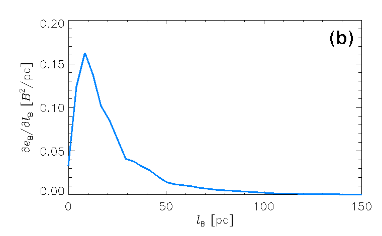
Figure 9.4: For Model ${\mathrm{B}1\rm{\Omega}}$ at $t=0.49\,{\rm Gyr}$ (a) the proportion of ${\langle\,{e_{\rm B}}\rangle}$ contribution from ${B}_{\ell}$ and ${b}$ depending on $\ell_{B}$ and (b) $\upartial{\langle\,{e_{\rm B}}\rangle}/\upartial\ell_{B}$. Compare with Fig. 8.2 for Model ${\mathrm{B}2\rm{\Omega}}$.

Table 9.2: Growth rate for the mean ($\Gamma_{e}$) and fluctuating ($\gamma_{e}$) magnetic energy during a portion of the kinematic stage for each model. $\hat{\Gamma}$ is the estimated growth rate of the mean magnetic field using the approximation described in Section 8.3. $\Delta t$ is the period analysed, and $N$ is the number of snapshots used. The fit of the sum of both exponentials to the total measured field energy is indicated by the reduced $\chi^{2}$.

Model	$2\hat{\Gamma}$	$\Gamma_{e}$	$\gamma_{e}$	$\Delta t$	$\chi^{2}$	$N$
	$[Gyr^{-1}]$	$[Gyr^{-1}]$	$[Gyr^{-1}]$	$[Gyr]$
${\mathrm{B}1\rm{\Omega}}$	0.0 – 1.4	2.1	2.6	0.4 – 0.83	0.42	31
${\mathrm{B}1\rm{\Omega}\rm{O}}$	0.0 – 1.4	10.1	9.0	0.4 – 0.70	0.01	16
${\mathrm{B}1\rm{\Omega}\rm{SN}}$	0.0 – 1.4	4.2	2.4	0.4 – 0.82	0.43	36
${\mathrm{B}2\rm{\Omega}}$	0.8 – .10	5.5	5.1	0.4 – 0.84	0.04	37
${\mathrm{B}1\rm{\Omega}\rm{Sh}}$	1.8 – 3.8	5.8	5.3	0.4 – 0.82	0.10	36

The growth rates of the mean and fluctuating parts of the magnetic energy from the MHD models are listed in Table 9.2. The plots of the actual growth together with the fitted exponentials are displayed in Fig. 9.5. These can be compared to the growth rates of the total field energy shown in Fig. 9.1b, which includes the whole simulation period. The table data and the plots in Fig. 9.5 are derived over a time interval of about $400\,{\rm Myr}$, and strong temporal fluctuations are evident, even over so long a time frame. This time frame is chosen because it is well within the kinematic regime for analysis of the dynamo, and because there is snapshot data for all models during this period. From the steady growth in Models ${\mathrm{B}1\rm{\Omega}\rm{O}}$ and ${\mathrm{B}2\rm{\Omega}}$ (panels a and b) it is clear that they can be well approximated as exponential. This is less clear from the other models (in panels c and d), which have more pronounced dips and plateaux. However from Fig. 9.1 it is evident that further exponential growth follows. There would be greater certainty over the parameters derived for $\Gamma_{e}$ and $\gamma_{e}$ if resources permitted the extension of these models for at least another $400\,{\rm Myr}$, and preferably up to saturation.

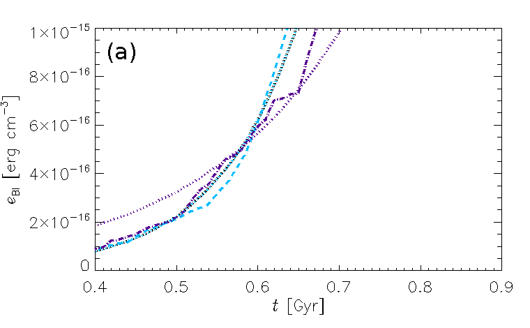
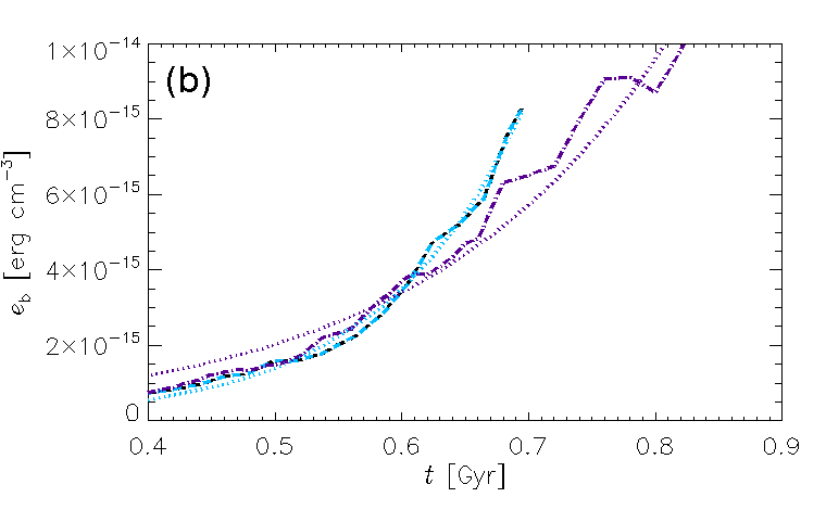
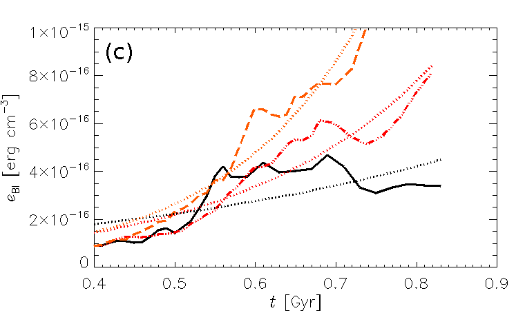
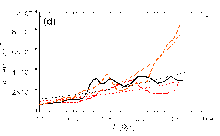
Figure 9.5: Growth of the mean ((a) and (c)) and fluctuating ((b) and (d)) field. Models ${\mathrm{B}1\rm{\Omega}\rm{O}}$ (light blue, dashed) and ${\mathrm{B}2\rm{\Omega}}$ (purple, dash-dotted) are shown in panels (a) and (b); Models ${\mathrm{B}1\rm{\Omega}}$ (black, solid), ${\mathrm{B}1\rm{\Omega}\rm{SN}}$ (red, dash-3dotted) and ${\mathrm{B}1\rm{\Omega}\rm{Sh}}$ (orange, long-dashed) in panels (c) and (d). Plotted with the actual growth rates are the exponential fits for each model (matching color, dotted). The parameters of the fits are detailed in Table 9.2.

The estimate $\hat{\Gamma}$ is derived using Eq.(8.7) from Section 8.3. The estimates included are $l_{\rm turb}=0.1\,{\rm kpc}$, $u_{\rm turb}=15\,{\rm km\,s^{-1}}$, $h=0.6\,{\rm kpc}$ and $D_{\textrm{crit}}=6\sim 10$. From the location of the strongest field in Fig. 9.2 it may be that for the mean field dynamo, the active region is $0.2\,\hbox to0.0pt{\raise 2.15277pt\hbox{$<$}\hss}{\lower 4.30554pt\hbox{$\sim$}}\,|z|\,\hbox to0.0pt{\raise 2.15277pt\hbox{$<$}\hss}{\lower 4.30554pt\hbox{$\sim$}}\,0.6$ with the mid-plane more active for the fluctuation dynamo. The height of the strongest mean field in Model ${\mathrm{B}1\rm{\Omega}\rm{SN}}$ appears slightly lower, $h\,\hbox to0.0pt{\raise 2.15277pt\hbox{$<$}\hss}{\lower 4.30554pt\hbox{$\sim$}}\,0.4\,{\rm kpc}$, from its equivalent plot to Fig. 9.2. This might be expected as the reduced SN activity will not inflate the disc as much. Otherwise $h$ appears quite consistent across the models. $l_{\rm turb}$ would not appear to be dependent upon the parameters, but on the size of the remnants. Again, it might be expected to be somewhat smaller for Model ${\mathrm{B}1\rm{\Omega}\rm{SN}}$, because increased density in the most SN active region could restrict typical remnant size. Since the gas in all models is transonic, the characteristic turbulent velocity is likely to be around the speed of sound for the gas. $u_{\rm turb}$ may therefore vary modestly and it will be worth obtaining improved approximations.

Comparing the model fitted growth rates $\Gamma_{e}$ to the estimates for the growth rates from the shear dynamo $\hat{\Gamma}$ all of the actual growth rates exceed the estimates, except for Model ${\mathrm{B}2\rm{\Omega}}$. In Section 8.3 this model was analysed for a later period in its evolution and $\Gamma_{e}=10.9\,{\rm Gyr}^{-1}$ obtained is comparable to $2\hat{\Gamma}=8\sim 10\,{\rm Gyr}^{-1}$. Perhaps there remains significant transients from the Model ${\mathrm{B}1\rm{\Omega}}$ snapshot at $400\,{\rm Myr}$ from which this model is initialised. Otherwise the model growth rates are only slightly above the upper estimates, except for Model ${\mathrm{B}1\rm{\Omega}\rm{O}}$ with $\Gamma_{e}=10.1\,{\rm Gyr}^{-1}$ much larger than the upper estimate of 1.4. This model has the open vertical boundary condition for the magnetic field and the efficiency of the dynamo may benefit from the advection of helicity.

Also of interest, the model growth rates $\gamma_{e}$ for the fluctuating field energy are generally smaller than for the mean field energy. This is not the case for Model ${\mathrm{B}1\rm{\Omega}}$ where $\Gamma_{e}=2.1\,{\rm Gyr}^{-1}$ is less than $\gamma_{e}=2.6\,{\rm Gyr}^{-1}$. As can be seen from Fig. 9.5c and d, the growth of this model had stalled temporarily, so this might not be significant over the longer times scales. For Model ${\mathrm{B}1\rm{\Omega}\rm{SN}}$ the relative difference between $\gamma_{e}=2.4\,{\rm Gyr}^{-1}$ and $\Gamma_{e}=4.2\,{\rm Gyr}^{-1}$ is somewhat larger than in the other models. This could also be due to the short term dip in the total magnetic energy, but may indicate a higher SN rate contributes to the fluctuation dynamo. In both cases further extended analysis in the kinematic phase is required.

9.3 Three-phase structure of the Field

The total volume probability distributions for gas number density $n$, temperature $T$ and thermal pressure $p$ are displayed in Fig. 9.6 from Models ${\mathrm{B}1\rm{\Omega}}$ (black, solid) and ${\mathrm{H}1\rm{\Omega}}$ (blue, dashed). Note that Model ${\mathrm{H}1\rm{\Omega}}$ includes the correction to the SN distribution, which stabilises the disc against unphysical cyclic oscillations, although it is still subject to natural random vertical fluctuations. Hence the mean density in the SN active region remains consistently higher than in Model WSWa.

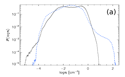
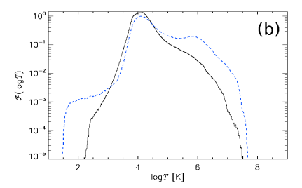
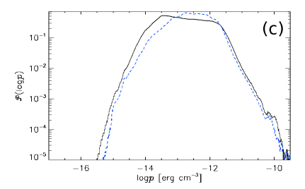
Figure 9.6: Volume weighted probability distributions of gas number density (a), temperature (b) and thermal pressure (c) for models ${\mathrm{H}1\rm{\Omega}}$ (black, solid) and ${\mathrm{B}1\rm{\Omega}}$ (blue, dashed) for the total numerical domain $|z|\leq 1.12\,{\rm kpc}$.

Although the three phase temperature distribution is still visible for this model in Fig. 9.6b, it is less pronounced than the results from Model WSWa shown in Fig. 5.3b. However the three phase structure for the MHD Model ${\mathrm{B}1\rm{\Omega}}$ is not at all apparent in panel b, with a significantly narrower range of temperatures. The bulk of the density distributions (a) are quite similar between the HD and MHD models, except that the high densities are not as well resolved in the MHD models. The thermal pressure distributions are very similar, but with the HD modal pressure approximately one third the MHD modal pressure.

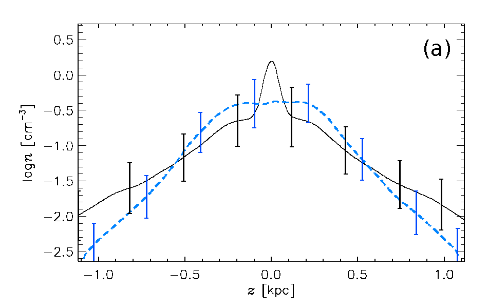
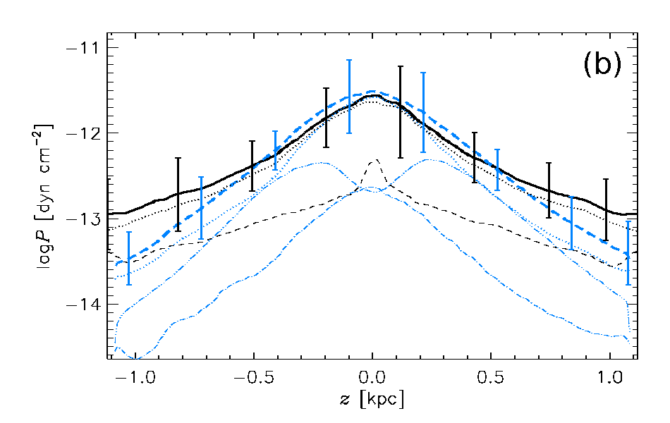
Figure 9.7: Horizontal averages of gas number density, $\overline{n}(z)$ (a), and total pressure, $\overline{P}(z)$ (b), for Model ${\mathrm{B}1\rm{\Omega}}$ (solid, black), and Model ${\mathrm{H}1\rm{\Omega}}$ (dashed, blue). Each are time-averaged using eleven snapshots respectively, spanning 100 Myr. The vertical lines indicate standard deviation within each horizontal slice. The thermal $\overline{p}(z)$ (dotted) and ram $\overline{p}_{\rm turb}(z)$ (fine dashed) pressures are also plotted (b). For Model WSWah the magnetic pressure $\overline{p}_{B}$ is also plotted (fine, dash-3dotted).

As discussed in Section 7.2 the stability of the disc reduces the effectiveness of the SNe to generate and circulate hot gas, in the absence of SN clustering. Hence Model ${\mathrm{H}1\rm{\Omega}}$ has a slightly thicker disc, with less hot gas than Model WSWa. On top of this the effect of the magnetic pressure in Model ${\mathrm{B}1\rm{\Omega}}$ is to expand the thick disc even further and this is illustrated in Fig. 9.7a, where the horizontal averages of gas number density $n(z)$ are plotted against $z$ for both models. The strong peak in the density at the mid-plane is evident for Model ${\mathrm{H}1\rm{\Omega}}$ (black, solid), while for Model ${\mathrm{B}1\rm{\Omega}}$ (blue, dashed) there is a broad plateau in the density, extending to $|z|\simeq 300\,{\rm pc}$, where the mean magnetic field is strongest.

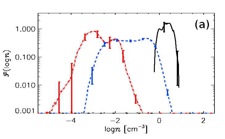
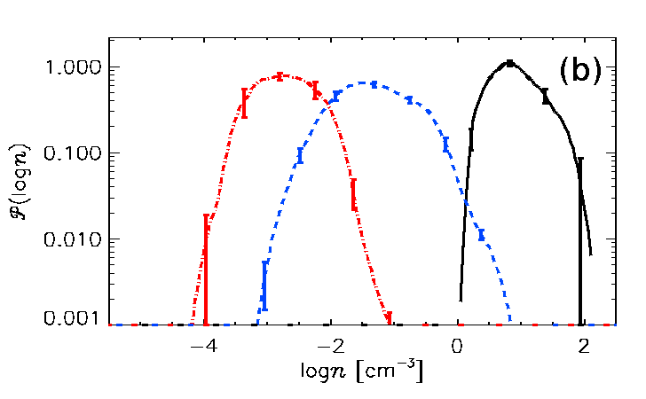
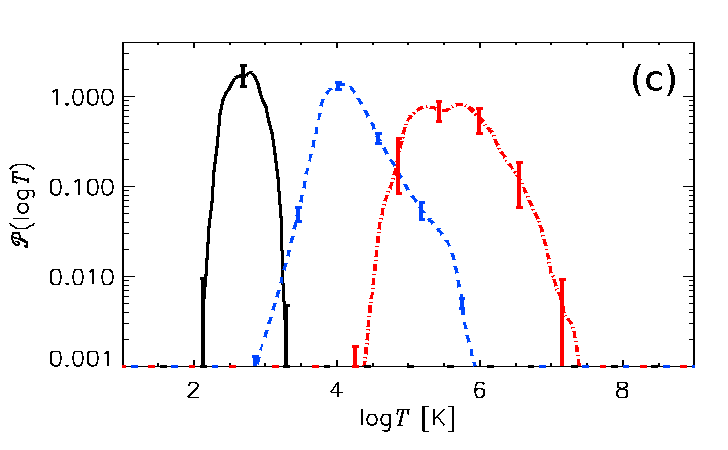
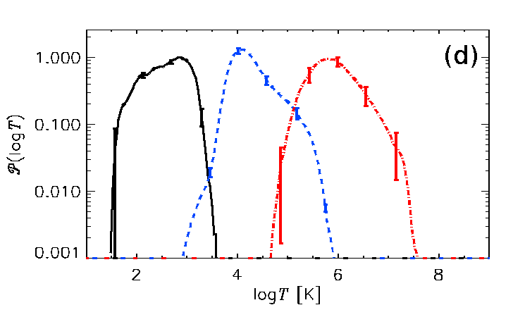
Figure 9.8: Probability distributions by phase: cold (blue, dashed), warm (black, solid) and hot (red, dash-dotted) for gas number density ($n$ (a), (b)) and temperature ($T$ (c), (d)) for Model ${\mathrm{B}1\rm{\Omega}}$ ((a), (c)) and Model ${\mathrm{H}1\rm{\Omega}}$ ((b), (d)). 95% confidence intervals for temporal deviation are shown as error bars.

The horizontal averages of the pressure are plotted in Fig. 9.7b for both models. There is a strong peak at the mid-plane in the turbulent pressure for the HD model (black, dashed), but a much weaker profile for the MHD model (blue, dash-dotted). There are two peaks in the magnetic pressure (blue, dash-3dotted) near $|z|\simeq 200\,{\rm pc}$, which supports the extended density profile. Another possible effect, which might constrain the circulation of the hot gas, and hence enhance the pressure at the mid-plane, is the strong horizontal orientation of the field. As mentioned in Section 9.1 the periodic boundary conditions exclude a non-zero vertical component to the mean field, so the magnetic tension predominantly acts against the vertical flows. Some understanding of the multi-phase structure of the magnetised ISM is still possible from these models, but the extreme temperatures and densities are significantly under represented. To improve this in future work it will be desirable to allow unrestricted evolution of vertical field and to apply realistic clustering of the SNe to generate more supperbubbles (composite multiple SN remnants forming a single superstructure) or chimneys (plumes venting hot gas from the disc towards the halo).

Results for separation of the ISM into three phases using the method detailed in Section 5.3 are shown for Models ${\mathrm{B}1\rm{\Omega}}$ and ${\mathrm{H}1\rm{\Omega}}$ in Fig 9.8 with total volume probability distributions. The phases are defined using entropy $s$ such that for cold $s<4.4\cdot 10^{8}\,{\rm erg}\,{\rm g}^{-1}\,{\rm K}^{-1}$ and hot $s>23.2\cdot 10^{8}\,{\rm erg}\,{\rm g}^{-1}\,{\rm K}^{-1}$ with warm in between. Apart from the higher densities for the cold phase with the HD model (panel b), anticipated by the volume distributions (Fig. 9.6), the warm and hot distributions for the MHD density (panel a) are broad, with a bimodal structure to the hot gas. The distributions for the warm gas (panels c and d) are very similar and for the cold (hot) distributions the MHD model does not extend to as low (high) temperatures.

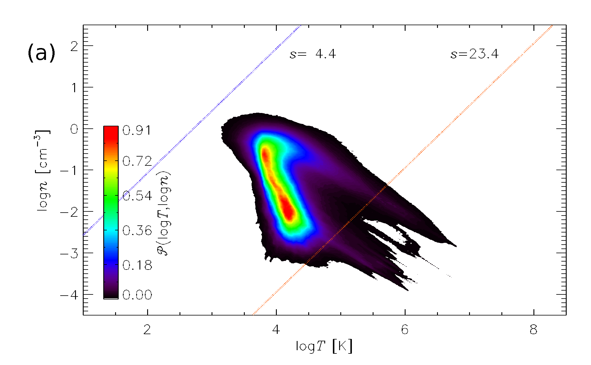
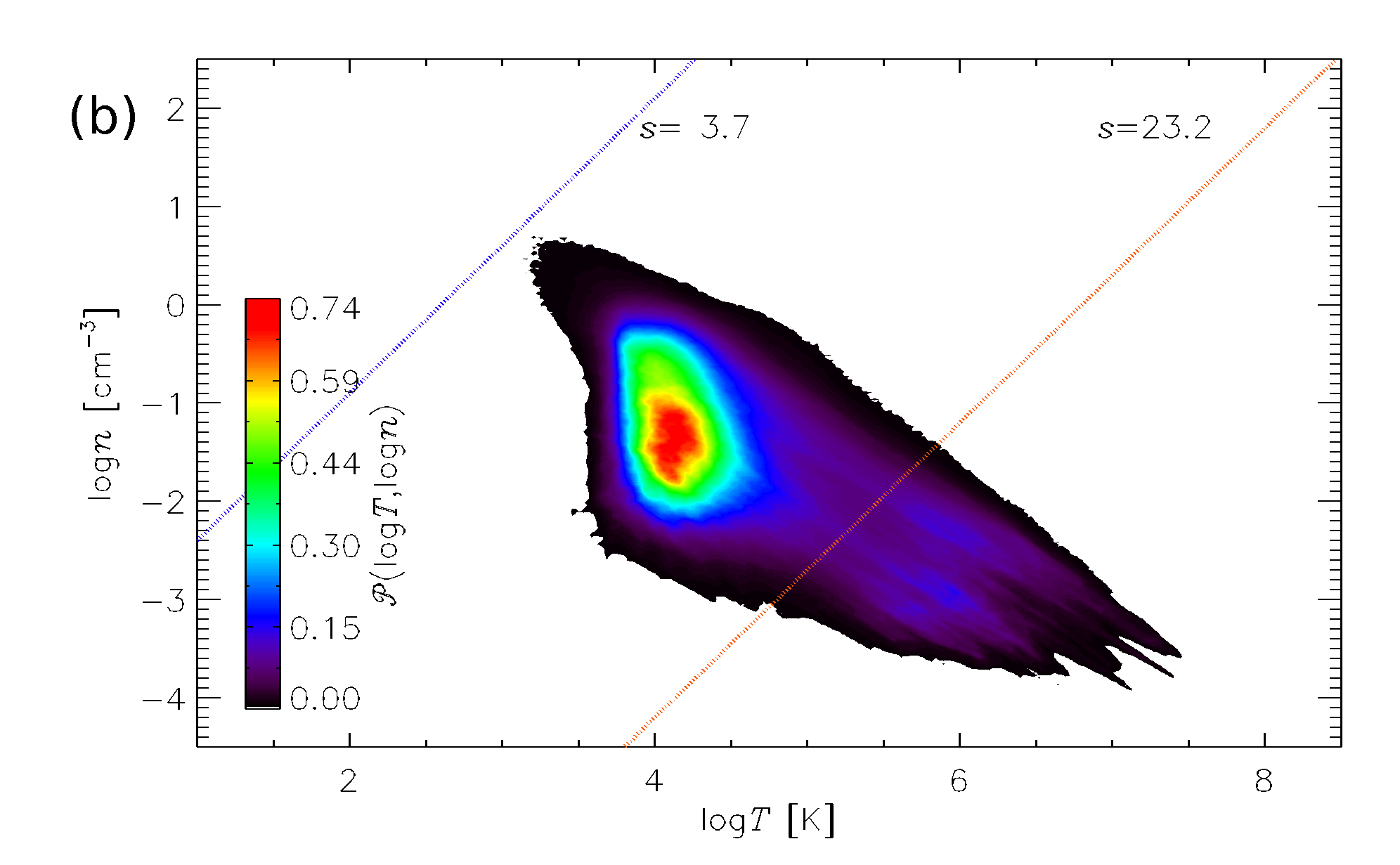
Figure 9.9: Probability contour plot by volume of log$n$ vs log$T$ for Model ${\mathrm{B}1\rm{\Omega}}$ (a) and Model ${\mathrm{H}1\rm{\Omega}}$ (b). The lines of constant entropy $s=4.4\cdot 10^{8}$ and $23.2\cdot 10^{8}\,{\rm erg}\,{\rm g}^{-1}\,{\rm K}^{-1}$ indicate where the phases are defined as cold for $s\leq 4.4$ and as hot for $s>23.2$.

Comparing the combined probability distribution of density and temperature for both of these models in Fig. 9.9 with those of Model WSWa in Fig. 5.4 the spread is more broad and not obviously aligned along a line of constant pressure. The HD distribution here is less compact than with MHD. However when considering only the mid-plane distributions, as displayed in Fig. 9.10 the distributions match better with Model WSWa and the pressure alignment is evident. So the broad distributions for the total volumes are explained by the stronger gradient in the pressure distribution, due to the reduced stirring of the hot gas. The thermal pressure at the mid-plane is also very similar in both models, reflected also in the agreement of the total and thermal pressure near the mid-plane in the plot of horizontal averages (Fig 9.7b). The magnetic and turbulent pressure in Model ${\mathrm{B}1\rm{\Omega}}$ combine to match the mid-plane turbulent pressure alone of Model ${\mathrm{H}1\rm{\Omega}}$. For the temperature in Model ${\mathrm{B}1\rm{\Omega}}$ the hot gas has two modes, evident in Fig. 9.9a at $10^{5}\,{\rm K}$ and $10^{6}\,{\rm K}$, but at the mid-plane there only the single $10^{3}\,{\rm K}$ mode. The structure of the ISM at the mid-plane is therefore common to both models with modes at $10^{6}\,{\rm K},~{}10^{-2}\,{\rm cm^{-3}}$ and $10^{4}\,{\rm K},~{}1\,{\rm cm^{-3}}$. The cold gas is insufficiently resolved in Model ${\mathrm{B}1\rm{\Omega}}$ for comparison.

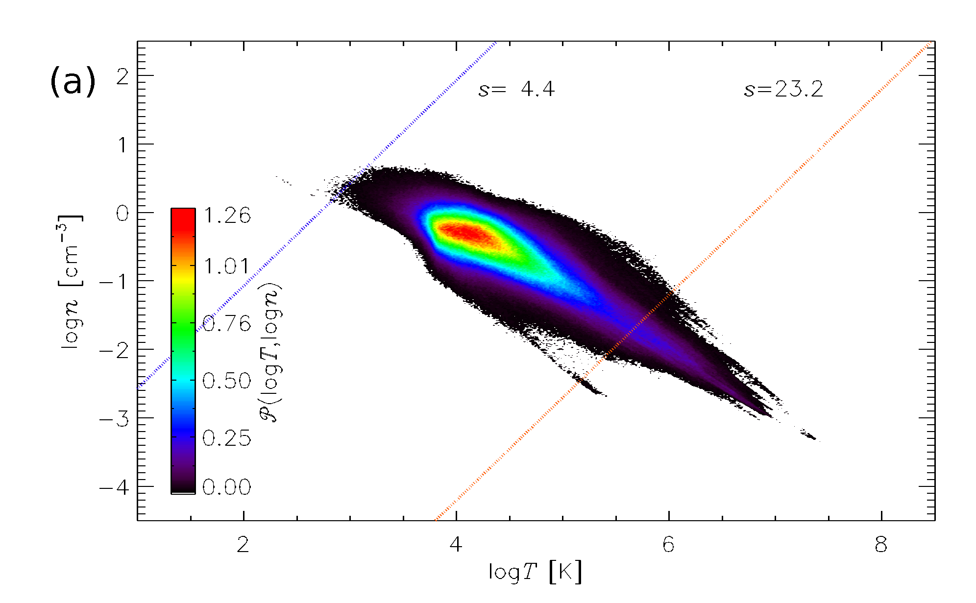
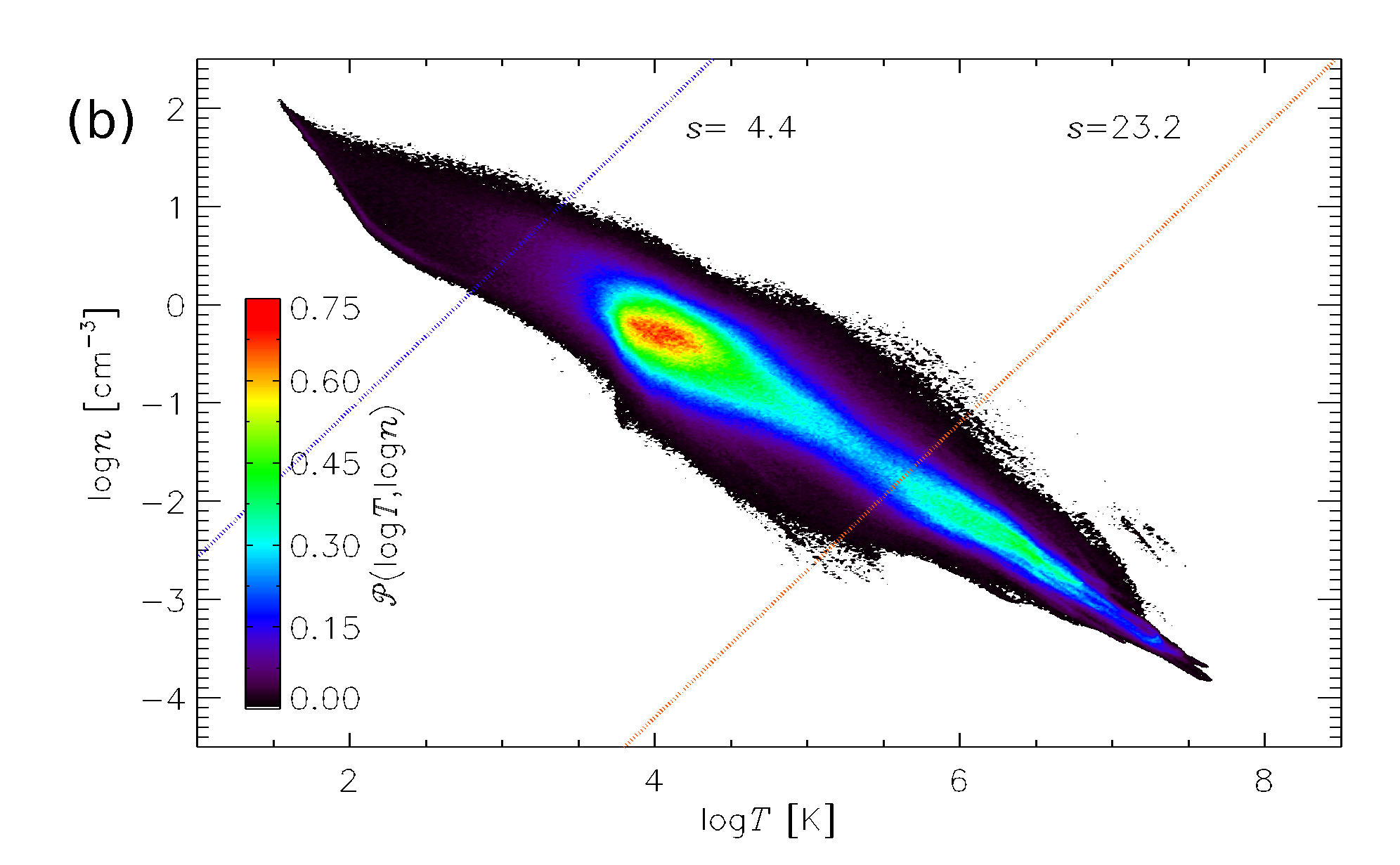
Figure 9.10: The mid-plane probability distributions ($|z|<100\,{\rm pc}$) by gas number density $\log n$ and temperature $\log T$ for (a) Model ${\mathrm{B}1\rm{\Omega}}$ and (b) Model ${\mathrm{H}1\rm{\Omega}}$.

There is no evident dependence in the probability distributions between the MHD models differing in rotation, shear or SN rate. The models in the kinematic stage extend to lower densities and higher temperatures than either the HD Model ${\mathrm{H}1\rm{\Omega}}$ or the MHD models in the dynamo saturated state, and also extend to lower pressures.

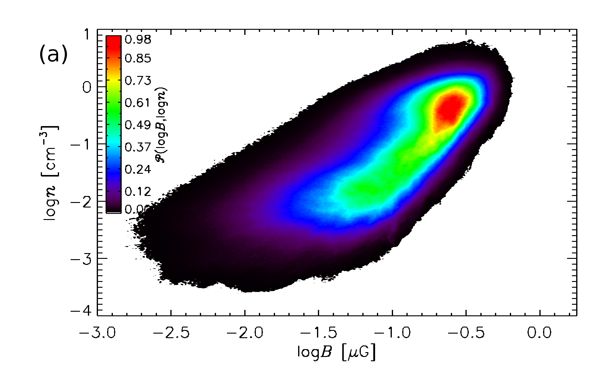
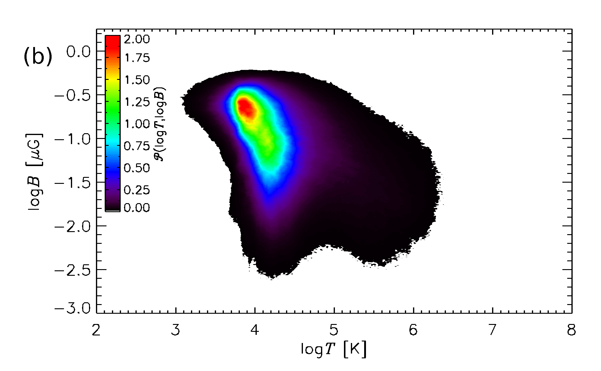
Figure 9.11: Total volume probability distributions ($|z|<100\,{\rm pc}$) by gas number density $\log n$ and magnetic field strength $\log|B|$ (a) and temperature $\log|T|$ and magnetic field strength $\log|B|$ (b) for Model ${\mathrm{B}1\rm{\Omega}}$.

In Fig. 9.11a the joint probability distributions of gas number density with magnetic field strength is shown and in Fig. 9.11b of temperature with magnetic field strength for Model ${\mathrm{B}1\rm{\Omega}}$. From (a) it is clear there is a strong positive correlation between magnetic field strength and density and from (b) a weak negative correlation between temperature and field strength. The $T,B$ distribution has very strong peak at $T=10^{4}\,{\rm K}$.

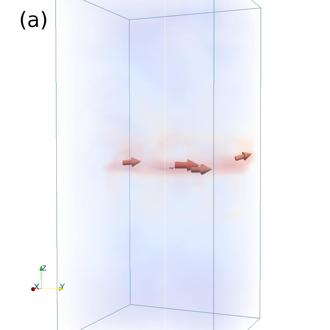
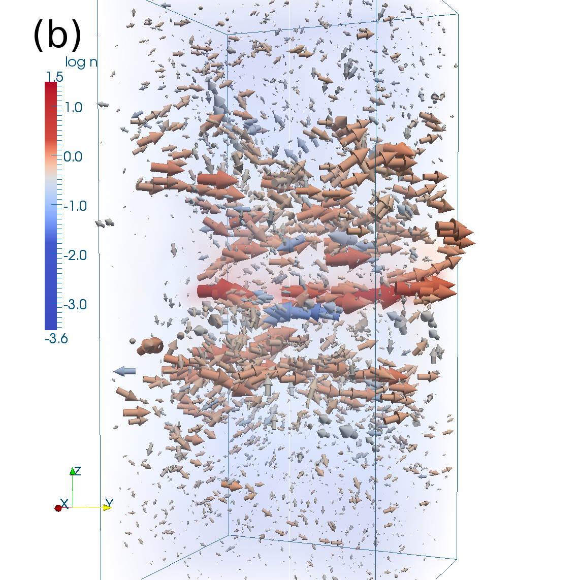
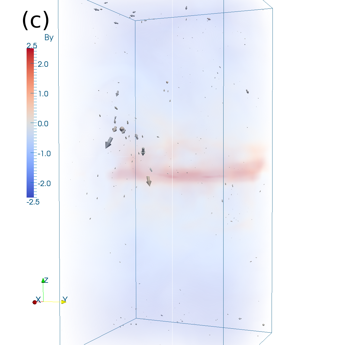
Figure 9.12: Vector plots of the magnetic field $B$ (a) in the cold phase (b) the warm phase and (c) the hot phase. Field directions are indicated by arrows and strength by their thickness. The colour of the arrows indicates the strength of the azimuthal ($y$) component (colour bar on the right). The background shading illustrates the density of the ISM.

For Model ${\mathrm{B}1\rm{\Omega}}$ the ISM for a single snapshot is decomposed into the three phases and the magnetic field for each plotted separately in Fig. 9.12. In panel a the cold gas occupies only a limited volume near the mid-plane, but the magnetic field is very strong and organised in alignment with the mean field surrounding it in the warm gas. This is represented by the length and thickness of the vector arrows. The colour of the arrows emphasises that the alignment has a strong azimuthal component. No arrows are present away from the mid-plane, because the cold gas is absent there. In panel b the warm gas is present throughout the numerical volume. Field vectors are present almost throughout and the field is highly aligned, mainly in the azimuthal direction. The strength of the field increases towards the mid-plane. The presence of some vectors in blue or grey indicates that there are significant perturbations where the field includes reversals, some of these strong. Some of the field exhibits significant vertical orientation, but it is mainly horizontal. In panel (c) the hot gas is also present throughout the volume, although in smaller amounts near the mid-plane. Despite this there is very little magnetic field. What field there is generally weak and lacks much systematic alignment, although any orientation tends to be vertical, consistent with the field lines being stretched by the gas flowing away from the mid-plane. Effectively the hot gas has a very weak field, which is highly disordered. Most of the magnetic field, and particularly the mean field, occupies the warm gas. Detailed quantitative analysis of the structure of the gas will be deferred to future work.

9.4 Structure of the Field

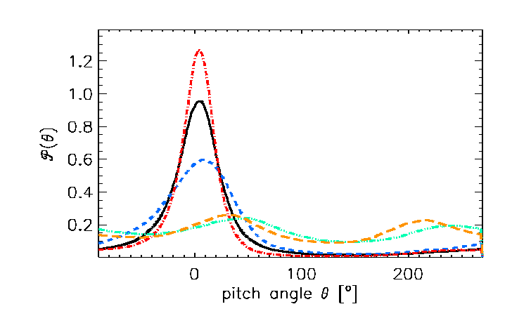
Figure 9.13: Total volume weighted probability distributions of magnetic field pitch angles in models ${\mathrm{B}1\rm{\Omega}}$ (black, solid), ${\mathrm{B}1\rm{\Omega}\rm{O}}$ (blue, dashed), ${\mathrm{B}2\rm{\Omega}}$ (red, dash-dotted), ${\mathrm{B}1\rm{\Omega}\rm{SN}}$ (green, dash-3dotted) and ${\mathrm{B}1\rm{\Omega}\rm{Sh}}$ (orange, long-dashed). Composite data for eleven snapshots each spanning $100\,{\rm Myr}$ from the saturated dynamo (kinematic stage) for the first three (latter two).

In future work the structure of the magnetic field shall be analysed in more depth for the total field as well as each phase individually. The correlation of the field in the kinematic stage and once the dynamo has saturated shall be measured, with attention to how it varies with height.

As a preliminary inspection the pitch angles, $\arctan(B_{x}/B_{y})$, for the total volume have been calculated for each model using eleven snapshots spanning $100\,{\rm Myr}$ and the probability distributions plotted in Fig. 9.13. As the dynamo evolves the magnetic field becomes increasingly ordered, with the orientation close to the azimuthal. Model ${\mathrm{B}2\rm{\Omega}}$ (red,dash-dotted), with the double rotation rate, predictably has the most regular field, with the smallest standard deviation and smallest modal pitch angle of $\theta\simeq 3^{\circ}$, close to the azimuthal direction. Increased rotation will increase the laminar tendency of the flow, whereas Models ${\mathrm{B}1\rm{\Omega}}$ (black, solid) and ${\mathrm{B}1\rm{\Omega}\rm{O}}$ (blue, dashed) have higher perturbation velocities relative to their rotation. So although the modal pitch angles are also close to azimuthal, $4^{\circ}$ and $9^{\circ}$ respectively, their standard deviations are higher. With open boundaries Model ${\mathrm{B}1\rm{\Omega}\rm{O}}$ the field is more irregular than Model ${\mathrm{B}1\rm{\Omega}}$.

In the kinematic stage for Models ${\mathrm{B}1\rm{\Omega}\rm{SN}}$ (green, dash-3dotted) and ${\mathrm{B}1\rm{\Omega}\rm{Sh}}$ (orange, long-dashed) the fields are clearly less organised and the modal pitch angles are further from the azimuthal with $\theta\simeq 50^{\circ}$ and $32^{\circ}$ respectively. There are also significant modes in almost the reverse directions, at $\theta\simeq 240^{\circ}$ and $216^{\circ}$ respectively. This is consistent with the higher magnitude of the relative helicity during the dynamo growth stage, as there is likely to be reduced tangling of the field lines if they have the same horizontal orientation. It may be, however, that the highly ordered field in these simulations is enhanced by the reduced motions of the hot gas. The lack of clustering in the SNe, now that the mass in the disc is more stable, and the constraint for the mean magnetic field to have zero vertical component, due to the periodic boundary conditions (Sections 7.2 and 9.1), mitigate against the transport of hot gas away from the disc. However the pitch angles may be expected to align within the range $9^{\circ}$ to $32^{\circ}$, assuming more scattering than in the saturated stage with Model ${\mathrm{B}1\rm{\Omega}\rm{O}}$ for the former and more ordering than in the kinematic stage for Model ${\mathrm{B}1\rm{\Omega}\rm{Sh}}$ for the latter angle.

9.5 Summary

All of the models investigated have produced a galactic mean field dynamo. In general the simulation dynamo grows more rapidly than the analytic predictions, so there would appear to be an additional elements in the theoretical model required to explain the dynamo. The efficiency of the dynamo is improved if positive magnetic helicity can be removed, either by vertical transport or resistive diffusion. The magnitude of the magnetic field is strongly aligned to the density of the ISM and indirectly the warm and cold phases. More particularly the mean field is stronger in the warm and cold gas, with the hot gas containing a more random field. The mean magnetic field and the magnetic energy is strongest at $|z|\simeq 300\,{\rm pc}$, just outside the SNe active region. The fluctuating dynamo is likely to be strongest in this SNe active region, but due to the low magnetic Reynolds numbers in the simulations, it is likely that the field and energy is significantly weaker in the simulations than might be expected.

Part VI Summary of results and future investigation

Chapter 10 Summary of results

10.1 Multi-phase ISM results

The multi-phase gas structure obtained in these simulations appears robust, relatively insensitive to the physical parameters included: total gas density or prescription of radiative cooling (Section 7.1), SN rates, or rates of rotation and shear (Section 9.3). Previous studies (e.g. Mac Low et al., 2005; Joung and Mac Low, 2006) indicate that the existence of such a multi-phase structure does not have as a prerequisite either rotation, shear or stratification. Its morphology, however, would strongly be affected by the latter. Only SN rates close to the Milky Way estimates have been considered here, so whether there are upper and lower rates where a multi-phase structure may be excluded, remains to be investigated.

The parameterization of the radiative cooling is especially important for the hot phase of the ISM. Apart from the obvious effect that there is more hot gas with the cooling function WSW, which has weaker cooling than RBN at $T\,\hbox to0.0pt{\raise 2.15277pt\hbox{$>$}\hss}{\lower 4.30554pt\hbox{$\sim$}}\,10^{3}\,{\rm K}$ (Fig. 3.1), regions of low thermal and total pressure are more widespread with RBN (Fig. 7.8). For the same reason, the WSW cooling function produces an ISM which has three times more thermal and kinetic energy than RBN (Fig. 7.4). However, with either cooling function, thermal energy is about twice the kinetic energy due to perturbation velocities; more work is needed to decide if the relation $E_{\mathrm{th}}\simeq 2E_{\mathrm{kin}}$ is of a general character.

Examination of the 2D probability distribution of $T$ and $n$, as described in Section 5.3, permits a physically motivated identification of natural boundaries of the major phases. Further refinement, distinguishing the SN active region $|z|\,\hbox to0.0pt{\raise 2.15277pt\hbox{$<$}\hss}{\lower 4.30554pt\hbox{$\sim$}}\,200\,{\rm pc}$ from the more homogeneous strata $|z|\,\hbox to0.0pt{\raise 2.15277pt\hbox{$>$}\hss}{\lower 4.30554pt\hbox{$\sim$}}\,200\,{\rm pc}$ (Section 5.1) improves the quality of the statistical modelling of each phase. The probability distribution of the density of each phase is approximated to high quality by lognormal fits.

Considering that probability densities for gas temperature and number density, calculated for individual phases, are clearly separated, it is significant that probability densities for both thermal and total pressure — the sum of thermal, magnetic (for MHD) and turbulent pressures — are not segregated at all. Despite its complex thermal and dynamical structure, the gas is in statistical pressure equilibrium. Since the SN-driven ISM is random in nature, both total and thermal pressure fluctuate strongly in both space and time (albeit with significantly smaller relative fluctuations than the gas density, temperature and perturbation velocity), so the pressure balance is also statistical in nature. These might appear to be obvious statements, since a statistically steady state (i.e., not involving systematic expansion or compression) must have such a pressure balance. However, alternative conclusions may be drawn that the broadness of the pressure distribution in itself, irrespective of the convergence of modal pressures, indicates thermal pressure disequilibrium and a single phase ISM. Systematic deviations from pressure balance may be associated with the vertical outflow of the hot gas (leading to lower pressures), and with the compression of the cold gas by shocks and other converging flows (leading to somewhat increased pressures). If we allow for the global vertical pressure gradient (cf. Fig. 5.7) it is evident that locally phases are in total pressure equilibrium and a multiphase description is useful for analysis of the ISM.

A direct relationship between various methods of estimating the filling factor or fractional volume from observations is presented in Section 5.2. If an appropriate means of relating the observable filling factor to the filling factor derived from the statistical properties of the distributions can be found — perhaps by applying the simulation model fits — then a more accurate estimate of the fractional volume of the various phases may emerge. This represents an improvement upon the assumption of locally homogeneous gas, the primary analytical tool used to date in determinations of the fractional volumes of the phases.

The modal properties of density, temperature, velocity, magnetic field, Mach number and pressure have been calculated for each phase separately. In particular there is confirmation that the phases, with quantifiable small intersections in terms of thermal and density distributions, are close to both thermal and total statistical pressure balance. Statistical modelling, as used for the density, is also possible for any magnetohydrodynamic variable. This provides the opportunity to identify regions of the ISM with diagnostics other than temperature or density, which may help to characterize the dominant phase within observations.

The correlation scale of the random flows is obtained in Section 6.2, from the autocorrelation functions of the velocity components. Within $200\,{\rm pc}$ of the mid-plane, the horizontal velocity components have a consistent correlation scale of about $100\,{\rm pc}$. In contrast, the scale of the vertical velocity (which has a systematic part due to the galactic outflow of hot gas) grows from about $100\,{\rm pc}$ at the mid-plane to nearly $200\,{\rm pc}$ at $z=200\,{\rm pc}$, and further at larger heights. This is due to the increase of the fractional volume of the hot gas with distance from the mid-plane. Near to $|z|\simeq 1\,{\rm kpc}$ (and beyond), most of the volume is occupied by the hot gas. Further measurements of the correlation scale above $500\,{\rm pc}$ are required to assess to what extent such flows may reliably be modelled within a numerical domain with horizontal dimensions of $1\,{\rm kpc}$.

There is clear indication of cold gas falling back towards the mid-plane at speeds of a few km/s, hot gas involved in vigorous outflow away from the mid-plane, and some warm gas entrained in this outflow (Section 6.1). The outflow speed of the hot gas increases up to $100\,{\rm km\,s^{-1}}$ within $100\,{\rm pc}$ of the mid-plane, and then slowly decreases. In contrast, the mean vertical velocity of the warm gas increases linearly with $|z|$, up to $20\,{\rm km\,s^{-1}}$ at $|z|=1\,{\rm kpc}$.

10.2 Magnetized ISM results

The strongest result from the MHD models is the successful generation of a mean field dynamo for all the parameters considered, including parameters matching the local Galaxy (Section 9.1). A fluctuating dynamo may also be present, but further analysis is required. In addition, an effective approach for identifying appropriately the mean and random elements of the magnetic field has been identified, in terms of local volume averaging (Section 8). The growth rates of the mean field and the fluctuating field for each model have been compared with analytic estimates for the shear dynamo appropriate for the parameters in each case, and the simulation results either match or exceed these estimates. The growth rates obtained exclude neither the possibility of a primordial field, nor a randomly seeded field via a Biermann battery. However the persistent orientation of the resultant mean field, without reversals in the azimuthal direction, is consistent with the hypothesis that galactic magnetic fields are generated through a dynamo, with the same alignment above and below the mid-plane and independent of galactic longitude (i.e. quadrupolar).

In these simulations the presence of positive magnetic helicity appears to limit the dynamo growth. Model ${\mathrm{B}1\rm{\Omega}\rm{O}}$, with open vertical boundary conditions, had more rapid growth magnetic field than the otherwise equivalent Model ${\mathrm{B}1\rm{\Omega}}$, with the vertical field condition on these boundaries. Although the former vents net magnetic energy through the external boundaries, which should slow the dynamo, it also expels significant positive magnetic helicity, which appears to enhance the dynamo. Otherwise all models generate net negative magnetic helicity on the resistive time-scale during the kinematic phase; this process is reversed as the dynamo saturates, reverting to a net relative helicity of approximately zero. The vertical transport of the magnetic field lines, and the associated sign dependent helicity, is therefore a persistent feature of the galactic dynamo; and significantly, the sign of the outward helicity flux is common to both sides of the mid-plane.

Analysis of the multiphase structure of the magnetic field indicates that the strength of the magnetic field is closely connected with the density, and by association the warm and cold phases of the ISM. Examination of the structure of this field in each phase reveals that the weak field in the hot gas is predominantly random. There is a very strong regular component to the field in the cold gas, organised and amplified in alignment with the ambient warm gas. Most of the mean field is present within the warm gas.

10.3 Future investigation and experiments

An important technical aspect of simulations of this kind is the minimum numerical resolution $\Delta$ required to capture the basic physics of the multi-phase ISM. As with all other simulations of the SN-driven ISM, a host of numerical tools (such as shock-capturing diffusivity) need to be employed to handle the extremely wide dynamical range (e.g. $10^{2}\,\hbox to0.0pt{\raise 2.15277pt\hbox{$<$}\hss}{\lower 4.30554pt\hbox{$\sim$}}\,T\,\hbox to0.0pt{\raise 2.15277pt\hbox{$<$}\hss}{\lower 4.30554pt\hbox{$\sim$}}\,10^{8}\,{\rm K}$ in terms of gas temperature and $10^{-4}\,\hbox to0.0pt{\raise 2.15277pt\hbox{$<$}\hss}{\lower 4.30554pt\hbox{$\sim$}}\,n\,\hbox to0.0pt{\raise 2.15277pt\hbox{$<$}\hss}{\lower 4.30554pt\hbox{$\sim$}}\,10^{2}\,{\rm cm}^{-3}$ gas number density within the model) and widespread shocks characteristic of the multi-phase ISM driven by SNe (detailed in Section 3.4). $\Delta=4\,{\rm pc}$ has been demonstrated to be sufficient with the numerical methods employed here, and results shown to be consistent with those obtained by other authors using adaptive mesh refinement with maximum resolutions of $2\,{\rm pc}$ and $1.25\,{\rm pc}$ (Section 5.1). The numerical method has been carefully tested by reproducing, quite accurately, the Sedov–Taylor and snowplough analytical solutions for individual SN remnants (Appendix A). Progress has been made in describing the multi-phase ISM structure and modelling the galactic dynamo in the vicinity close to the mid-plane. The relatively low vertical boundary, with carefully applied vertical boundary conditions, has adequately captured the critical features of the SN-driven ISM.

From the data already available through these simulations, considerable additional analysis would prove interesting. The distribution of the gas number density and its description in terms of lognormal fits has been considered, and a similar treatment of other measurables, such as temperature, gas speed and pressure should also be possible. Some analysis of the total velocity correlation scales has been reported, but it would be useful to conduct this analysis of the gas velocity by individual phases, to identify the correlation scale for each. It would also be useful to investigate the correlation of time and position of the velocity field. The forcing by SN turbulence against a background of stratification and differential rotation induces a combination of vortical and divergent velocity. How these are decomposed within the velocity field, and how their interaction is affected by changing the rates of SN injection, or galactic rotation, might help to understand how the galactic dynamo operates.

Simulated line-of-sight observation from any location within a simulation, considering local bubbles, and taking into account changes in elevation, would permit us to compare simulated observational measurements with direct data measurements, and extend the ways in which observational measurements might be interpreted, with regard to underlying processes. This would be particularly useful in terms of Faraday rotation measures for the magnetic field. All of the models so far have parameters close to the solar neighbourhood, so the statistics could be readily identified with observational data.

Building upon the existing model, a number of future extensions present themselves.

Parameter Sweep

To understand the effects of various parameters requires each parameter to be considered for a range of values; at least three each, and preferably more. So the rates of SN injection, rotation and shear need to be varied separately to identify how these affect the properties of the ISM.

The model need not be restricted to galaxies similar to the Milky Way. Galaxies at higher redshift (young galaxies) could be investigated using different stellar gravitational potentials and higher proportions of ISM to stars.

Supernova Rates

Currently the models are constructed with the SN rates imposed as a parameter, based on a multiple of the observed SN rates. The Schmidt-Kennicutt Law (Kennicutt, 1998) defines a relationship between the gas surface density of the galactic disc with an SN rate, which is a reasonable fit to the data from observations. Some numerical models on the scale of galaxies have successfully reproduced star-formation and feedback rates which reasonably match this relationship dynamically, rather than by imposition (e.g. Dobbs, Burkert and Pringle, 2011). At the local level, however, how the distribution of gas within cold clouds (rather than the bulk volume of the gas in the warm ISM) is related to the supernova rate is highly non-trivial.

Nevertheless it would be preferable to derive a method of SN feedback, which responds to the mass available for star formation, and the distribution of the gas between the cold and warm phases; i.e a system in which the SN rate is self-regulating, slowing down if SN activity burns aways the gas, and speeding up as gas cools into clouds and star formation increases. Such an experiment may require a reasonably well modelled galactic fountain and an appropriate scheme for including realistic clustering of the SNe, to facilitate the venting of the hot gas from the disc as discussed in Section 7.2. Given the rarefaction of the gas density across the disc, due to spiral arms and other effects, it is not immediately apparent how such locally determined supernova rates might relate to the Schmidt-Kennicutt Law, applicable to the whole galaxy. However, experiments with a range of gas density distributions representative of the spiral arm (inter arm) regions could be considered, in which the Schmidt-Kennicutt relations might be a lower (upper) bound against which to assess the algorithm. An effective self-regulating method, which is reasonably consistent with the Schmidt-Kennicutt Law, would then be a useful analytical tool to apply in galaxies with a broad range of parameters, which may differ significantly from the local Galaxy.

Vertical Magnetic Field

As discussed in Section 9.1, the contraint that ${\langle B_{z}\rangle}=0$ is a construct of the periodic boundary conditions rather than a physical result. To explore the natural evolution of the vertical structure of the magnetic field, which is poorly understood due to difficulty in deriving observational measurements, alternative horizontal boundary conditions are required. Keeping the horizontal boundary condition on $A_{z}$ periodic or sheared would not affect $B_{z}$, but will contribute to the horizontal components and retain the effect of shear on $B_{x}$. With appropriate care to handle shocks crossing the boundary, setting the first or second derivatives for $A_{x}$ and $A_{y}$ to zero, should permit $B_{z}$ to evolve naturally.

Allowing the mean field to have a vertical component will also relax the horizontal magnetic tension and allow greater, more physical circulation of gas between the disc and halo. Given that the objective here will be to understand the structure of the field, the net flow of magnetic energy across the boundaries is of less concern, so the open field condition on the vertical boundary should be employed, as applied for Model ${\mathrm{B}1\rm{\Omega}\rm{O}}$, so as not to constrain $B_{x}$ and $B_{y}$ nonphysically.

Cosmic Rays

Cosmic rays are estimated to account for about one quarter of the pressure in the ISM, and are strongly aligned with the magnetic field. Including them effectively will allow results from the simulations to be much more directly compared with observational estimates, including the vertical distribution of density, temperature and pressure, and fitted values of the probability distributions of these variables. The interaction of cosmic rays with thermodynamics and hydrodynamics has not previously been explored on these scales, so subtle or even dramatic effects may be revealed.

In addition, synchrotron emissions are an important tool for observations, and modelling these directly via simulated line-of-sight measurements will improve the comparison with the real observations. We shall also be able to compare the simulated observations with the direct measurements, to assess how robust the observational assumptions are.

Galactic Fountain

de Avillez and Breitschwerdt (2007) and similar models have sufficient vertical extent with $|z|=10\,{\rm kpc}$ for hot gas to cool and recycle naturally to the mid-plane. With their limited horizontal aspect, however, we cannot know enough about the true scales of the galactic fountain. With the grid scale $\Delta$ varying in the vertical direction and increasing the horizontal range of the model, I intend to explore the physical and time scales of the galactic fountain. Due to the damping effect of the magnetic field, it may paradoxically be numerically more efficient to include magnetism for this project, and possibly also cosmic rays, rather than to model a purely hydrodynamic regime.

Spiral Arms

The range of models included so far assume the gas is located in an inter arm region of the galaxy. There are no density waves encountered as the numerical box orbits the galactic centre. How the formation of stars, generation and orientation of the magnetic field reacts within and between the spiral arms is not well understood. Within this model, spiral arms could be modelled with an additional gravitational potential which passes through the box at set times during its orbit.

Parker and Magnetorotational Instability and SN Quenching

Parker instabilities occur in plasma subject to gravitational forces, and magnetorotational instabilities occur in differentially rotating plasma. These instabilities are postulated to be damped by the turbulence generated by SNe. These models could be used to test this postulation by simulating a system in which either or both of these instabilities are present. Repeating the experiment in each case, with and without SN driven turbulence included, it would be possible to identify whether the instabilities are in fact suppressed.

10.4 Review

In conclusion, such models are highly complex in their construction, and in the results they generate. The results reported in this thesis are the product of several revised sets of calculations, possible only after many sets of simulations that preceded them. Changes take hundreds of thousands of iterations to unfold, and it is not always immediately apparent which outcomes are robust physical effects and which are numerical artifacts. Given that the observational data and theoretical framework is far from complete, it is also not always obvious whether the numerical results, which appear to match our expectations of the ISM, are in fact true, or results which appear to conflict with our expectations are nevertheless correct.

The more the results have been analysed, the better our understanding of the model and the causes of various effects. It would be desirable to be able to run all the simulations with exactly the same numerical ingredients, but such is the expense in resources and time that as improvements and corrections are revealed they are implemented on the fly, and cannot often be applied retrospectively. Hence there are considerable algorithmic differences between the HD models and the MHD models; and even within the sets of simulations, some numerical ingredients differ, beyond the physical parameters which are under investigation.

This is a new model and with each set of simulations, better experience is garnered on how best to interpret and report the results. It is now a very rich numerical resource, which has the potential to unlock far more secrets of the ISM than have been listed in this thesis. I hope to have the opportunity to extend this model in the directions described above, and in the process to shed new light on the structure and dynamics of galaxies.

Appendix A Evolution of an individual supernova remnant

A.1 The snowplough test

The thermal and kinetic energy supplied by SNe drives, directly or indirectly, all the processes discussed in this thesis. It is therefore crucial that the model captures correctly the energy conversion in the SN remnants and its transformation into the thermal and kinetic energies of the interstellar gas. As discussed in Section 3.2, the size of the region where the SN energy is injected corresponds to the adiabatic (Sedov–Taylor) or snowplough stage. Given the multitude of artificial numerical effects required to model the extreme conditions in the multi-phase ISM, it is important to verify that the basic physical effects are not affected, while sufficient numerical control of strong shocks, rapid radiative cooling, supersonic flows, etc., is properly ensured. Another important parameter to be chosen is the numerical resolution.

Before starting the simulations of the multi-phase ISM reported in this thesis, I have carefully verified that the model can reproduce, to sufficient accuracy, the known realistic analytical solutions for the late stages of SN remnant expansion, until merger with the ISM. The minimum numerical resolution required to achieve this in this model is $\Delta=4\,{\rm pc}$. In this Appendix, I consider a single SN remnant, initialised as described in Section 3.2, that expands into a homogeneous environment. All the numerical elements of the model are in place, but here periodic boundary conditions are used in all dimensions.

The parameters $\chi_{1}$ and $\nu_{1}$ are as applied in Model WSWa for $\Delta=4\,{\rm pc}$, but reduced here proportionally for $\Delta=2$ and $1\,{\rm pc}$. The constant $C\approx 0.01$ used in Eq. (3.10) to suppress cooling around shocks is unchanged. This may allow excess cooling at higher resolution, evident in the slightly reduced radii in Fig. A.1. For Model WSWah, $\chi_{1}$ and $\nu_{1}$ were just as in Model WSWa; for future reference, they should be appropriately adjusted, as should $C$, to better optimise higher resolution performance.

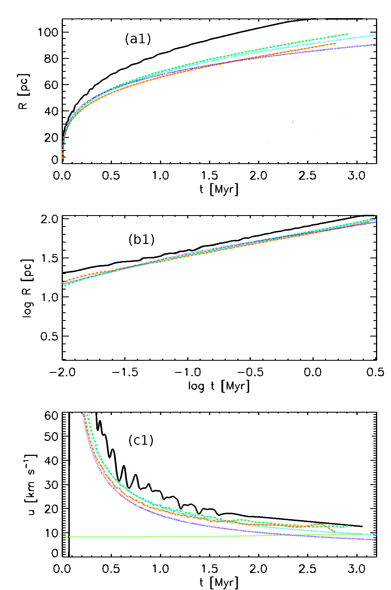
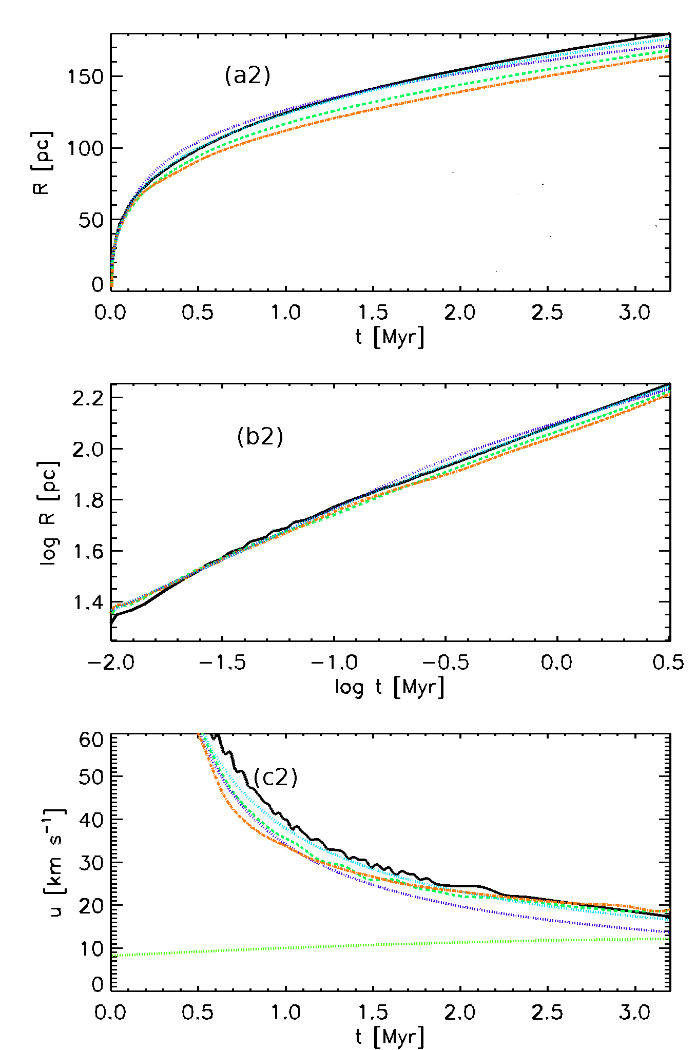
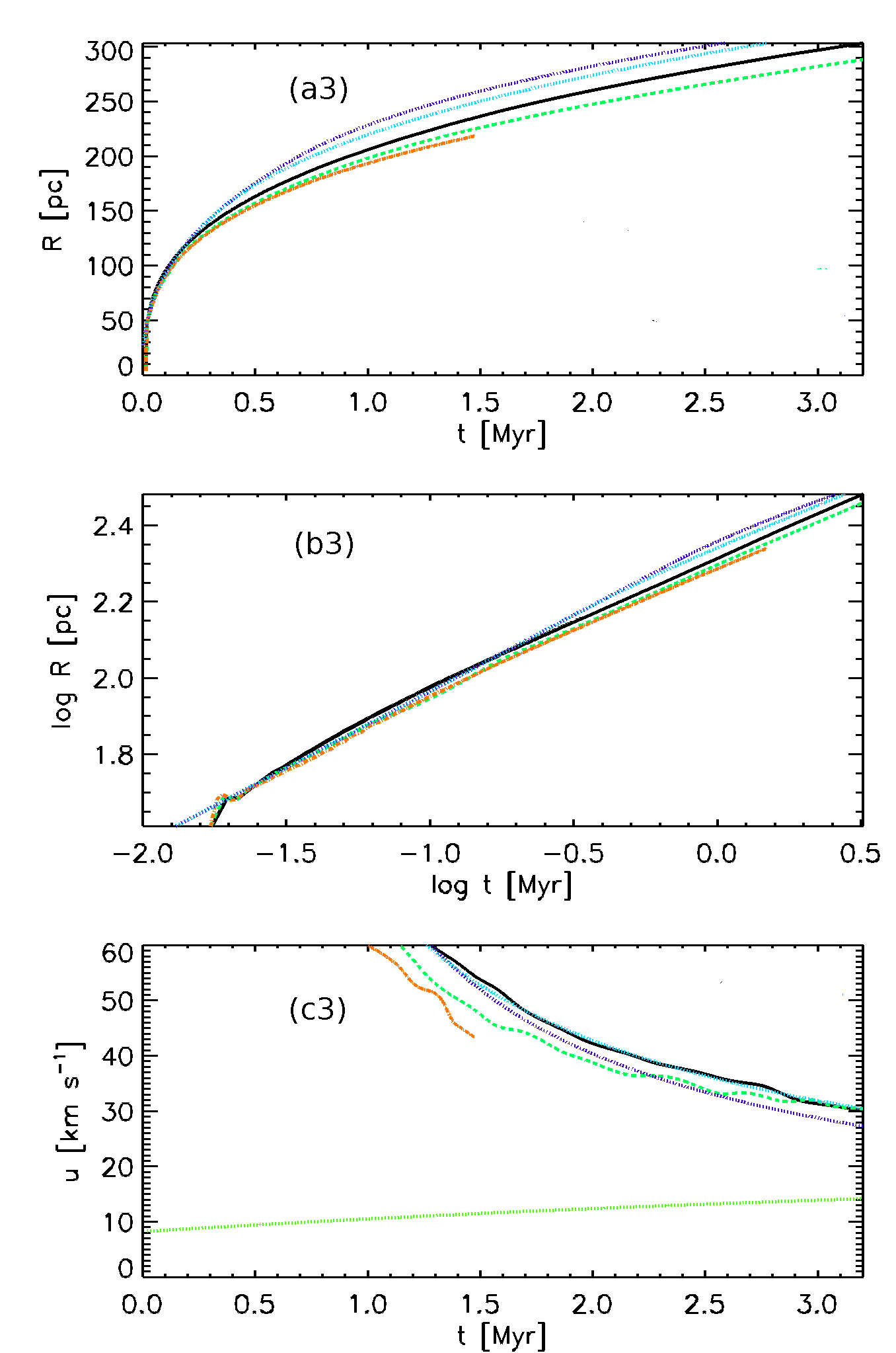
Figure A.1: The shell radius $R$ of an SN remnant versus time, shown in (a) linear and (b) logarithmic scales; (c) the corresponding expansion speed $\dot{R}$. Frame columns 1–3 are for different ambient gas densities, $\rho_{0}/10^{24}\,{\rm g}\,{\rm cm^{-3}}=(1.0,0.1,0.01)$ from left to right. Numerical results obtained under three numerical resolutions are shown: $\Delta=4\,{\rm pc}$ (black, solid), 2 pc (green, dashed) and 1 pc (orange, dash-dotted). Dotted lines are for the standard snowplough solution (A.2) (dark blue) and its modification by Cioffi, McKee and Bertschinger (1998) (light blue). The horizontal line in Panels (c1)–(c3) shows the sound speed in the ambient ISM.

The adiabatic and snowplough stages

The Sedov–Taylor solution,

$$R=\left(\kappa\frac{E_{\rm SN}}{\rho_{0}}\right)^{{1}/{5}}t^{{2}/{5}},$$ (A.1)

is accurately reproduced with this code at the resolution $\Delta=4\,{\rm pc}$ or higher. Here $R$ is the remnant radius, $E_{\rm SN}$ the explosion energy, $\rho_{0}$ the ambient gas density, and dimensionless parameter $\kappa\approx 2.026$ for $\gamma=5/3$ (Ostriker and McKee, 1988).

Modelling even a single remnant becomes more challenging when radiative cooling becomes important. Here numerical results are compared with two analytic solutions for an SN remnant expanding into a perfect, homogeneous, monatomic gas at rest. The standard momentum-conserving snowplough solution for a radiative SN remnant has the form

$$R=R_{0}\left[1+4\frac{\dot{R_{0}}}{R_{0}}(t-t_{0})\right]^{{1}/{4}},$$ (A.2)

where $R_{0}$ is the radius of the SN remnant at the time $t_{0}$ of the transition from the adiabatic stage, and $\dot{R_{0}}$ is the shell expansion speed at $t_{0}$. The transition time is determined by Woltjer (1972) as that when half of the SN energy is lost to radiation; this happens when

$$\dot{R_{0}}=230\,{\rm km\,s^{-1}}\left(\frac{n_{0}}{1\,{\rm cm^{-3}}}\right)^{{2}/{17}}\left(\frac{E_{\rm SN}}{10^{51}\,{\rm erg}}\right)^{{1}/{17}};$$ (A.3)

the transitional expansion speed thus depends very weakly on parameters.

Pressure driven and momentum driven snowplough

Cioffi, McKee and Bertschinger (1998) obtained numerical and analytical solutions for an expanding SN remnant with special attention to the transition from the Sedov–Taylor stage to the radiative stage. These authors adjusted an analytical solution for the pressure-driven snowplough stage to fit their numerical results to an accuracy of within 2% and 5% in terms of $R$ and $\dot{R}$, respectively. (Their numerical resolution was $0.1\,{\rm pc}$ in the interstellar gas and $0.01\,{\rm pc}$ within ejecta.) They thus obtained

$$R=R_{\rm{p}}\left(\frac{4}{3}\frac{t}{t_{\rm{p}}}-\frac{1}{3}\right)^{3/10},$$ (A.4)

where the subscript ${\rm{p}}$ denotes the radius and time for the transition to the pressure driven stage. The estimated time of this transition is

$$t_{\rm{p}}\simeq 13\,{\rm Myr}\left(\frac{E_{\rm SN}}{10^{51}\,{\rm erg}}\right)^{3/14}\left(\frac{n_{0}}{1\,{\rm cm^{-3}}}\right)^{-4/7}.$$

For ambient densities of $\rho_{0}=(0.01,0.1,1)\times 10^{-24}\,{\rm g}\,{\rm cm^{-3}}$, this yields transition times $t_{\mathrm{p}}\approx(25,6.6,1.8)\times 10^{4}\,{\rm yr}$ and shell radii $R_{\rm{p}}\approx(130,48,18)\,{\rm pc}$, respectively, with speed $\dot{R}_{\mathrm{p}}=(213,296,412)\,{\rm km\,s^{-1}}$.

This continues into the momentum driven stage with

$$\left(\frac{R}{R_{\rm{p}}}\right)^{4}=\frac{3.63~{}\left(t-t_{\rm{m}}\right)}{t_{\rm{p}}}\left[1.29-\left(\frac{t_{\rm{p}}}{t_{\rm{m}}}\right)^{0.17}\right]+\left(\frac{R_{\rm{m}}}{R_{\rm{p}}}\right)^{4},$$ (A.5)

where subscript ${\rm{m}}$ denotes the radius and time for this second transition,

$$t_{\rm{m}}\simeq 61\,t_{\mathrm{p}}\left(\frac{\dot{R}_{\rm{ej}}}{10^{3}\,{\rm km\,s^{-1}}}\right)^{3}\left(\frac{E_{\rm SN}}{10^{51}\,{\rm erg}}\right)^{-3/14}\left(\frac{n_{0}}{1\,{\rm cm^{-3}}}\right)^{-3/7},$$

where $\dot{R}_{\rm{ej}}\simeq 5000\,{\rm km\,s^{-1}}$ is the initial velocity of the $4M_{\odot}$ ejecta. For each $\rho_{0}=(0.01,0.1,1.0)\times 10^{-24}\,{\rm g}\,{\rm cm^{-3}}$, the transitions occur at $t_{\rm{m}}=(168,16.8,1.68)\,{\rm Myr}$, and $R_{\rm{m}}=(1014,281,78)\,{\rm pc}$, respectively. The shell momentum in the latter solution tends to a constant, and the solution thus converges with the momentum-conserving snowplough (A.2); but, depending on the ambient density, the expansion may become subsonic and the remnant merge with the ISM before Eq. (A.2) becomes applicable.

The simulation results are compared with the momentum-conserving snowplough solution and those of Cioffi, McKee and Bertschinger in Fig. A.1, testing the model with numerical resolutions $\Delta=1$, 2 and 4 pc for the ambient gas densities $\rho_{0}=(0.01,0.1,1.0)\times 10^{-24}\,{\rm g}\,{\rm cm^{-3}}$. Shown in Fig. A.1 are: a linear plot of the remnant radius $R$ versus time, to check if its magnitude is accurately reproduced; a double logarithmic plot of $R(t)$, to confirm that the scaling is right; and variation of the expansion speed with time, to help assess more delicate properties of the solution. There is good agreement with the analytical results for all the resolutions investigated when the ambient gas number density is below $1\,{\rm cm^{-3}}$. For $\Delta=4\,{\rm pc}$, the remnant radius is accurate to within about 3% for $\rho_{0}=10^{-25}\,{\rm g}\,{\rm cm^{-3}}$ and underestimated by up to 6% for $\rho_{0}=10^{-26}\,{\rm g}\,{\rm cm^{-3}}$. At higher numerical resolutions, the remnant radius is underestimated by up to 7% and 11% for $\rho_{0}=10^{-25}\,{\rm g}\,{\rm cm^{-3}}$ and $10^{-26}\,{\rm g}\,{\rm cm^{-3}}$, respectively. For $\rho_{0}=10^{-24}\,{\rm g}\,{\rm cm^{-3}}$, excellent agreement is obtained for the higher resolutions, $\Delta=1$ and $2\,{\rm pc}$; simulations with $\Delta=4\,{\rm pc}$ overestimate the remnant radius by about 20–25% in terms of $R$ and $\dot{R}$ at $t=2\,{\rm Myr}$. Note that a typical SN explosion site in the models described in the main part of the thesis has an ambient density $n_{0}<1\,{\rm cm^{-3}}$ so that $\Delta=2$ or $4\,{\rm pc}$ produce a satisfactory fit to the results, despite the much finer resolution of the simulations of Cioffi, McKee and Bertschinger.

The higher than expected expansion speeds into dense gas can be explained by the artificial suppression of the radiative cooling within and near to the shock front as described by Eq. (3.10). Our model reproduces the low density explosions more accurately because the shell density is lower, and radiative cooling is therefore less important.

A.2 Cooling-heating in the shocks

In code units, the applied net (heating or) cooling $([\Gamma-\rho\Lambda]~{}T^{-1})$ has amplitudes much greater than 1, and of opposite sign in close proximity. Perturbations to $\Gamma$ or $\Lambda$ are particularly vulnerable to instability when acted upon by shocks, and can lead to purely numerical thermal spikes, which can cause the code to crash. Therefore some form of suppression of net cooling within the shock profile is essential for code stability.

In addition, the method of enhanced diffusion coefficients for handling shocks has the effect of broadening the shock profiles and increasing the density spread. High density ISM inside the remnants cool faster, thus diffusing the hot phase ISM more rapidly than would occur within the unresolvable thin shock fronts that exist physically.

Having considered various approaches, a prescription is adopted which is stable, consistent with the snowplough, reduces cooling in the remnant shell interior, and applies cooling to the peak shell density. The net diffuse heating/cooling $[\Gamma-\rho\Lambda]~{}T^{-1}$ is multiplied by $\xi=e^{-C(\nabla\zeta)^{2}}$, where $\zeta$ is the shock diffusivity, defined in Eq. (3.9). Therefore, $\xi$ is unity through most of our domain, but reduces towards zero in strong shocks, where $(\nabla\zeta)^{2}$ is non-zero. $C$ is another numerical factor, the value of which is chosen to guarantee code stability without altering the basic physics; these constraints are normally fulfilled with $C\simeq 0.01$.

A.3 The structure of the SN remnant

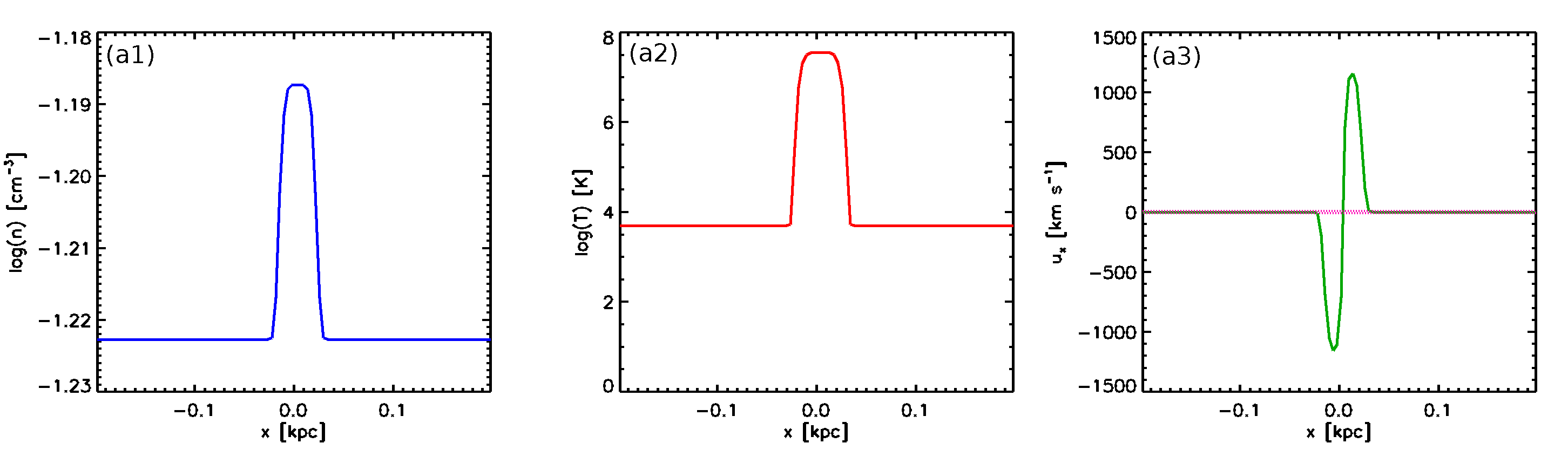
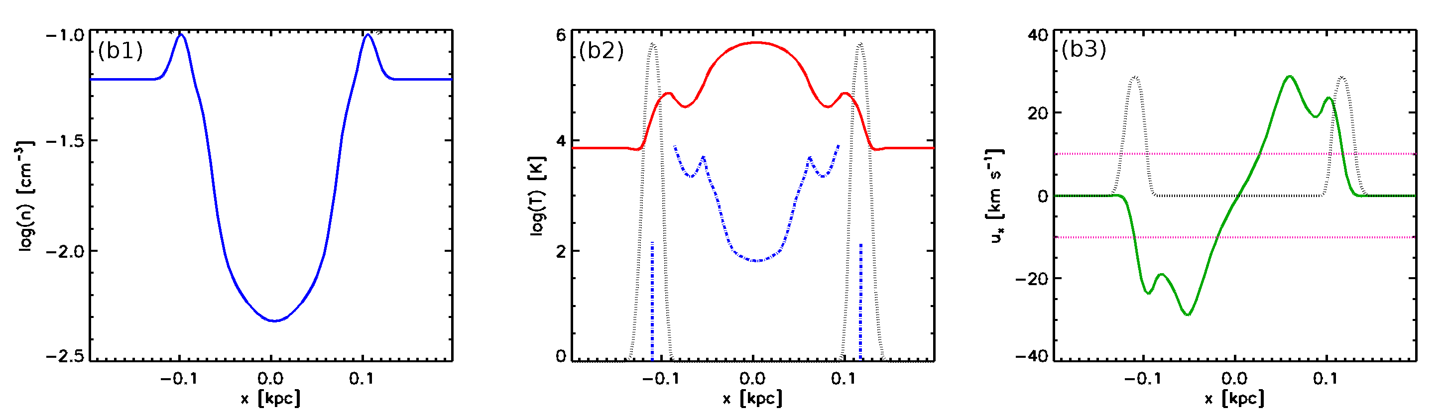
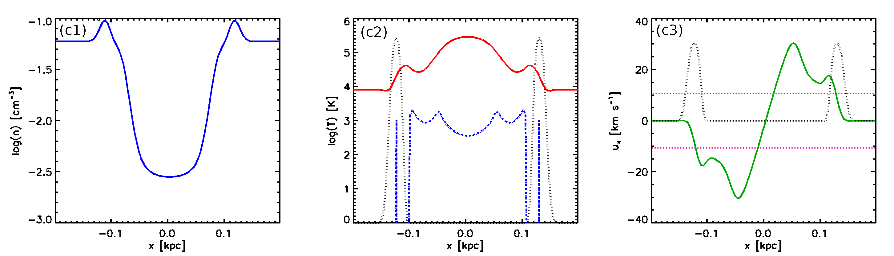
Figure A.2: One-dimensional cuts through the origin of an SN remnant expanding into gas of a density $\rho_{0}=10^{-25}\,{\rm g}\,{\rm cm^{-3}}$, simulated with the numerical resolution $\Delta=4\,{\rm pc}$. The variables shown are (a1)–(c1) gas density, (a2)–(c2) temperature, and (a3)–(c3) velocity. The shock viscosity profile of Eq. (3.9) (scaled to fit the frame, black, dotted) is shown in the temperature and velocity panels; the net cooling, log($-T^{-1}(\Gamma-\rho\Lambda)$), only where $\rho\Lambda\geq\Gamma$, from Eq. (3.1) (blue, dashed) is included in the temperature panel; and the ambient sound speed (pink, dashed) is also shown with the velocity. Panels in the top row (a) show the injection profiles used to initialise the remnant at $t=0$; the lower panel rows are for the later times (b) $t=0.72\,{\rm Myr}$ and (c) $t=1.02\,{\rm Myr}$.

Cuts through the simulated SN remnant are shown in Fig. A.2 for gas density, temperature and velocity, obtained for resolution $\Delta=4\,{\rm pc}$ and with ambient density $\rho_{0}=10^{-25}\,{\rm g}\,{\rm cm}^{-3}$. In the temperature and velocity panels, the profile of the shock viscosity from Eq. (3.9) is also included (black dotted line), scaled to fit each plot. The temperature panels also show where net cooling is applied to the remnant, $T^{-1}(\Gamma-\rho\Lambda)<0$ from Eq. (3.1) (blue dashed line), while the velocity panels also show the ambient sound speed (pink dashed lines). The top panel depicts the initial distributions, at $t=0$, with which the mass of $4{M_{\odot}}$ and $5\times 10^{50}\,{\rm erg}$ each of thermal and kinetic energy are injected. The other panels are for $t=0.72$ and $1.02\,{\rm Myr}$ after the start of the evolution, from top to bottom, respectively; the actual simulation continued to $t=1.32\,{\rm Myr}$, when the remnant radius reached $130\,{\rm pc}$.

The position of the peak of the density profile is used to determine the shell radius shown in Fig. A.1. The Rankine–Hugoniot jump conditions are not very well satisfied with the numerical parameters used here. This is due to our numerical setup, essentially designed to control the shocks by spreading them sufficiently to be numerically resolvable in production runs that contain many interacting shocks and colliding SN shells. Better shock front profiles have been obtained with other choices of parameters and cooling control, and with better resolution. The density and temperature contrasts across the shock fronts are reduced by the shock smoothing, which inhibits the peak density and enhances gas density behind the shocks. In an isolated remnant, the peak gas number density does not exceed $10\,{\rm cm^{-3}}$, but in the full ISM simulation densities in excess of $100\,{\rm cm^{-3}}$ are obtained, as a result of interacting remnants and highly supersonic flows.

The interior of the SN remnant, if more dense due to numerical smoothing about the shock profile, would cool unrealistically rapidly, so that the SN energy would be lost to radiation rather than agitate the ambient ISM. The centre panels in Fig. A.1 clarify how the cooling suppression described in Eq. (3.10) reduces the cooling rate in the relatively homogeneous interior of the remnant, while still allowing rapid cooling in the dense shell where the gradient of the shock viscosity is small. It is evident from the temperature cuts that the remnant still contains substantial amounts of hot gas when its radius reaches 100 pc, so it would be merging with the ISM in the full simulation.

The panels in the right column of Fig. A.2 demonstrate that the interior gas velocity can be more than twice the shell speed. Due to the high interior temperature, this flow is subsonic, while the remnant shell expands supersonically with respect to its ambient sound speed. The enhanced viscosity in the hotter interior (with viscosity proportional to the sound speed; see Section 3.4) inhibits numerical instabilities that could arise from the high velocities. In fact, accurate modelling of the SN interiors is not essential in the present context (where the main interest is in a realistic description the multi-phase ISM), as long as the interaction of the remnant with the ambient gas is well described, in terms of the energy conversion and transfer to the ISM, the scales and energy of turbulence, and the properties of the hot gas.

Appendix B Stability criteria

B.1 Courant criteria

Time step control

To achieve numerical stability with the explicit time stepping used, the Courant-Friedrichs-Lewy conditions have to be amply satisfied. For example, for advection terms, the numerical time step should be selected such that

$$\Delta t<\kappa\frac{\Delta}{\max(c{{}_{\mathrm{s}}},u,U)},$$

where $c{{}_{\mathrm{s}}}$ is the speed of sound, $u=|{{\mbox{\boldmath$u$}}}|$ is the amplitude of the perturbed velocity, i.e., the deviation from the imposed azimuthal shear flow $U$, and $\kappa$ is a dimensionless number, determined empirically, which often must be significantly smaller than unity. Apart from the velocity field, other variables also affect the maximum time step, e.g., those associated with diffusion, cooling and heating, so that the following inequalities also have to be satisfied:

$$\Delta t<\frac{\kappa_{1}\Delta^{2}}{\max(\nu,\gamma\chi,\eta)}\,,\quad\quad\Delta t<\frac{\kappa_{2}}{H_{\max}}\,,$$

where $\kappa_{1}$ and $\kappa_{2}$ are further empirical constants and

$$H_{\max}=\max\left(\frac{2\nu|\textbf{{W}}|^{2}+\zeta_{\nu}(\nabla\cdot{{\mbox{\boldmath$u$}}})^{2}+\zeta_{\chi}(\nabla\cdot{{\mbox{\boldmath$u$}}})^{2}}{\,{c_{\rm v}}T}\right)\,.$$

$\kappa=\kappa_{1}=0.25$ and $\kappa_{2}=0.025$ are used. The latter, more stringent constraint has a surprisingly small impact on the typical time step, but a large positive effect on the numerical accuracy. Whilst the time step may occasionally decrease to below 0.1 or 0.01 years following an SN explosion, the typical time step is more than 100 years.

Minimum diffusivity

Numerical stability also requires that the Reynolds and Péclet numbers defined at the resolution length $\Delta$, as well as the Field length, are sufficiently small. These mesh Péclet and Reynolds numbers are defined as

$${\rm Pe}{{}_{\Delta}}=\frac{u\Delta}{\chi}\leq\frac{u_{\rm{max}}\Delta}{\chi}\,,\quad{\rm Re}{{}_{\Delta}}=\frac{u\Delta}{\nu}\leq\frac{u_{\rm{max}}\Delta}{\nu}\,,$$ (B.1)

where $u_{\rm{max}}$ is the maximum perturbed velocity and $\Delta$ is the mesh length. For stability these must not exceed some value, typically between 1 and 10.

In numerical modelling of systems with weak diffusivity, $\nu$ and $\chi$ are usually set constant, close to the smallest value consistent with the numerical stability requirements. This level strongly depends on the maximum velocity, and hence is related to the local sound speed, which can exceed $1500\,{\rm km\,s^{-1}}$ in the ISM models. To avoid unnecessarily strong diffusion and heat conduction in the cold and warm phases, the corresponding diffusivity is scaled with gas temperature, as $T^{1/2}$. As a result, the diffusive smoothing is strongest in the hot phase (where it is most required). This may cause reduced velocity and temperature inhomogeneities within the hot gas, and may also reduce the temperature difference between the hot gas and the cooler phases.

The effect of thermal instability is controlled by the Field length,

$$\lambda_{\mathrm{F}} \simeq\left(\frac{KT}{\rho^{2}\Lambda}\right)^{1/2}\simeq 2.4\,{\rm pc}\left(\frac{T}{10^{6}\,{\rm K}}\right)^{\frac{7}{4}}\!\!\left(\frac{n}{1\,{\rm cm^{-3}}}\right)^{-1}\!\!\left(\frac{\Lambda}{10^{-23}\,{\rm erg}\,{\rm cm}^{3}\,{\rm s}^{-1}}\right)^{-\frac{1}{2}},$$

where any heating has been neglected. To avoid unresolved density and temperature structures produced by thermal instability, it is required that $\lambda_{\mathrm{F}}>\Delta$, and so the minimum value of the thermal conductivity $\chi$ follows as

$$\chi_{\mathrm{min}}=\frac{1-\beta}{\gamma\tau{{}_{\rm cool}}}\left(\frac{\Delta}{2\upi}\right)^{2},$$

where $\tau{{}_{\rm cool}}$ is the minimum cooling time, and $\beta$ is the relevant exponent from the cooling function (e.g. as in Table 3.2 for WSW cooling). In the single remnant simulations of Appendix A, $\tau{{}_{\rm cool}}\gtrsim 0.75\,{\rm Myr}$. In the full ISM simulations, minimum cooling times as low as $0.05\,{\rm Myr}$ were encountered. $\chi_{\mathrm{min}}$ has maxima corresponding to $\beta=0.56,-0.2,-3,\ldots$ for $T=313,10^{5},2.88\times 10^{5}\,{\rm K}\ldots$. All of these, except for that at $T=313\,{\rm K}$, result in $\chi_{\mathrm{min}}<4\times 10^{-4}\,{\rm km\,s^{-1}}\,{\rm kpc}$ at $c{{}_{\mathrm{s}}}=c_{1}=1\,{\rm km\,s^{-1}}$, so are satisfied by default for any $\chi_{1}$ sufficiently high to satisfy the ${\rm Pe}{{}_{\Delta}}\leq 10$ requirement. For $T=313\,{\rm K}$, at $c{{}_{\mathrm{s}}}=c_{1}$, then $\chi_{\mathrm{min}}=6.6\times 10^{-4}\,{\rm km\,s^{-1}}\,{\rm kpc}>\chi_{1}$. Thus if cooling times as short as 0.05 Myr were to occur in the cold gas, $\lambda_{\mathrm{F}}<\Delta$, and the model would be marginally under-resolved. Analysis of the combined distribution of density and temperature from Fig. (7.1), however, indicates that cooling times this short occur exclusively in the warm gas.

With $\chi_{1}\approx 4.1\times 10^{-4}\,{\rm km\,s^{-1}}\,{\rm kpc}$, as adopted in Section 3.4, then ${\rm Pe}{{}_{\Delta}}\leq 10$ is near the limit of numerical stability. (The choice of thermal diffusivity is discussed further in Appendix B.2.) As a result, the code may occasionally crash (notably when hot gas is particularly abundant), and has to be restarted. When restarting, the position or timing of the next SN explosion is modified, so that the particularly troublesome SN that causes the problem is avoided. In extreme cases, it may be necessary to increase $\chi$ temporarily (for only a few hundred time steps), to reduce the value of ${\rm Pe}{{}_{\Delta}}$ during the period most prone to instability, before the model can be continued with the normal parameter values.

B.2 Thermal Instability

One of the two cooling functions employed in this thesis, WSW, supports isobaric thermal instability in the temperature range $313<T<6102\,{\rm K}$ where $\beta<1$. (Otherwise, for the RBN cooling function or outside this temperature range for WSW cooling, $\beta\geq 1$ or $\Gamma\ll\rho\Lambda$, so the gas is either thermally stable or has no unstable equilibrium.)

Under realistic conditions for the ISM, thermal instability can produce very small, dense gas clouds which cannot be captured with the resolution $\Delta=4\,{\rm pc}$ used here. Although the efficiency of thermal instability is questionable in the turbulent, magnetized ISM, where thermal pressure is just a part of the total pressure (Vázquez-Semadeni, Gazol and Scalo, 2000; Mac Low and Klessen, 2004, and references therein), this instability is purposely suppressed in my model. However, this is done not by modifying the cooling function, but rather by enhancing thermal diffusivity so as to avoid the growth of perturbations at wavelengths too short to be resolved by the numerical grid.

Following Field (1965), consider the characteristic wave numbers

$$k_{\rho}=\frac{\mu(\gamma-1)\rho_{0}{\cal L}_{\rho}}{\mathcal{R}c{{}_{\mathrm{s}}}T_{0}},\quad k_{T}=\frac{\mu(\gamma-1){\cal L}_{T}}{\mathcal{R}c{{}_{\mathrm{s}}}},\quad k_{K}=\frac{\mathcal{R}c{{}_{\mathrm{s}}}\rho_{0}}{\mu(\gamma-1)K},$$

where $\mathcal{R}$ is the gas constant, and the derivatives $\mathcal{L}_{T}\equiv(\upartial\mathcal{L}/\upartial T)_{\rho}$ and $\mathcal{L}_{\rho}\equiv(\upartial\mathcal{L}/\upartial\rho)_{T}$ are calculated for constant $\rho$ and $T$, respectively. The values of temperature and density in these equations, $T_{0}$ and $\rho_{0}$, are those at thermal equilibrium, $\mathcal{L}(T_{0},\rho_{0})=0$ with $\mathcal{L}=\rho\Lambda-\Gamma$. Isothermal and isochoric perturbations have the characteristic wave numbers $k_{\rho}$ and $k_{T}$, respectively, whereas thermal conductivity $K$ is characterized by $k_{K}$. The control parameter of the instability is $\varphi=k_{\rho}/k_{K}$.

The instability is suppressed by heat conduction, with the largest unstable wave numbers given by (Field, 1965)

$$k_{\rm cc}= \left[k_{K}(k_{\rho}-k_{T})\right]^{1/2}\,,$$ (B.2)

$$k_{\rm cw}= \left[-k_{K}\left(k_{T}+\frac{k_{\rho}}{\gamma-1}\right)\right]^{1/2}\,,$$ (B.3)

for the condensation and wave modes, respectively, whereas the most unstable wave numbers are

$$k_{\rm mc}= \left[\frac{(1-\beta)^{2}}{\gamma^{2}}+\frac{\beta(1-\beta)}{\gamma}\right]^{1/4}(k_{\rho}k_{\rm cc})^{1/2}\,,$$ (B.4)

$$k_{\rm mw}= \left|\frac{\beta-1}{\gamma}\,k_{\rho}k_{\rm cw}\right|^{1/2}\,.$$ (B.5)

Table B.1: The unstable wavelengths of thermal instability, according to Field (1965), at thermally unstable equilibria $(T_{0},\rho_{0})$ with the WSW cooling function.

$T_{0}$	$\rho_{0}$	$\varphi$	$\lambda_{\rho}$	$\lambda_{\mathrm{cc}}$	$\lambda_{\mathrm{mc}}$	$\lambda_{\mathrm{cw}}$	$\lambda_{\mathrm{mw}}$
$[\!\,{\rm K}]$	[$10^{-24}\,{\rm g}/\!\,{\rm cm}^{3}$]		[pc]	[pc]	[pc]	[pc]	[pc]
313	4.97	1.91	002	05	005	02	004
4000	1.20	0.04	101	32	084	14	074
6102	0.94	0.02	192	44	136	20	120

Table B.1 contains the values of these quantities for the parameters of the reference Model WSWa, presented in terms of wavelengths $\lambda=2\upi/k$, rather than of wave numbers $k$. The unstable wavelengths of thermal instability are comfortably resolved at $T_{0}=6102\,{\rm K}$ and $4000\,{\rm K}$, with the maximum unstable wavelengths $\lambda_{\rm cc}=44\,{\rm pc}$ and $32\,{\rm pc}$, respectively, being much larger than the grid spacing $\Delta=4\,{\rm pc}$. The shortest unstable wavelength of the condensation mode in the model, $\lambda_{\rm cc}=5\,{\rm pc}$ at $T\approx 313\,{\rm K}$ is marginally resolved at $\Delta=4\,{\rm pc}$; gas at still lower temperatures is thermally stable. Unstable sound waves with $\lambda_{\rm cw}=2\,{\rm pc}$ at $T=313\,{\rm K}$ are shorter than the numerical resolution of the reference model. However, for these wave modes to be unstable, the isentropic instability criterion must also be satisfied, which is not the case for $\beta>0$, so these modes remain thermally stable.

Thus, there can be confidence that the parameters of these models (most importantly, the thermal diffusivity) have been chosen so as to avoid any uncontrolled development of thermal instability, even when only the bulk thermal conductivity is accounted for. Since much of the cold gas, which is most unstable, has high Mach numbers, thermal instability is further suppressed by the shock capturing diffusivity.

Appendix C Mass sensitivity and mass conservation

Effect of molecular mass

The two Models RB & WSWb have about 117% of the ISM mass of the reference Model WSWa, the difference corresponding to the abundance of molecular hydrogen. The difference is apparent comparing the lower panel of Fig. 7.5 with the upper panel of Fig. 5.12. Including the molecular gas, the abundance of hot gas reduces with height, contrary to observation, while otherwise it increases with height. Its inclusion appears to produce unrealistically strong cooling, as evident in the altered profiles of velocity and temperature in the horizontal averages of Fig. 5.2 from $t=400\,{\rm Myr}$, after the transition from Model WSWb to Model WSWa.

Therefore all the other models presented in this thesis match the mass in Model WSWa, assuming that the cloudy molecular component is concentrated in very small scales, not resolved by the coarse grid. Comparing the lower panels of Fig. 7.8 for WSWb with Fig. 5.5 for WSWa, the higher end of all three total pressure distributions are very similar, but for the warm and hot gas the distributions extend to much longer tails of low pressure gas. When molecular gas is included it appears that much of the gas is under pressured and out of equilibrium. Otherwise, comparing Fig. 7.8 with Fig. 5.5, the probability distributions for density, velocity and Mach numbers are very similar. The density distributions without the molecular hydrogen are narrower, but the peaks match, so aside from the pressures, the phase structure appears to be independent of the disc surface density.

Numerical mass diffusion

The Pencil code is non-conservative, so that gas mass is not necessarily conserved; this can be a problem due to extreme density gradients developing with widespread strong shocks. In general, solving Eq. (3.1) in terms of log density rather than linear density is numerically more efficient. However solving for $\rho$, rather than $\ln\rho$ is more accurate, and applying a numerical diffusion to the equation of mass resolves the problem of numerical dissipation in the snowplough test cases described in Appendix A.1, with mass then being conserved to within machine accuracy. Eq. (3.1) thus becomes

$$\frac{D\rho}{Dt}\,=\,-\nabla\cdot(\rho{{\mbox{\boldmath$u$}}})\,+\dot{\rho}_{\rm SN},+({\cal{V}}+\zeta_{\cal{V}})\nabla^{2}\rho+\nabla\zeta_{\cal{V}}\cdot\nabla\rho,$$ (C.1)

in which constant ${\cal{V}}\approx 4.1\times 10^{-3}\,{\rm km\,s^{-1}}\,{\rm kpc}$ is the unphysical mass diffusion coefficient and $\zeta_{\cal{V}}$ is as defined in Eq. (3.9), but with coefficient $c_{\cal{V}}=1$. A correction term is then required for mass conservation for each of Eq. (3.1) and (3.1).

$$\frac{D{{\mbox{\boldmath$u$}}}}{Dt}\longrightarrow\frac{D{{\mbox{\boldmath$u$}}}}{Dt}-\rho^{-1}\frac{{\cal{V}}\nabla^{2}\rho}{2}{{\mbox{\boldmath$u$}}}\,,\qquad\rho T\frac{Ds}{Dt}\longrightarrow\rho T\frac{Ds}{Dt}-\frac{{\cal{V}}\nabla^{2}\rho}{\,{c_{\rm p}}}.$$

However for the full model, once the ISM becomes highly turbulent, there remains some numerical mass loss. A comparison of mass loss through the vertical boundaries to the total mass loss in the volume indicates that numerical dissipation accounts for much less than 1% per $\,{\rm Gyr}$. The rate of physical loss, due to the net vertical outflow, is of order $15\%$ per $\,{\rm Gyr}$.

Boundary mass loss

In such a demanding simulation of this nature, it is inevitable that some heavily parameterized processes, approximations and numerical patches must be employed: cooling functions, supernova injection, boundary conditions and shock capturing viscosity amongst others, all of which have been explained and hopefully satisfactorily justified. Perhaps the most physically compromising numerical fix, which is necessary to maintain the mass in the long MHD runs, relates to the issue of physical boundary losses.

The general net outflow of gas through the vertical boundaries is a genuine physical process and consequence of sustained SN activity. Even if we were able to incorporate the galactic fountain and recycle this gas to the mid-plane, the loss of mass from the ISM would be entirely expected over a period of a few hundred Myr, never mind a Gyr. The natural evolution of a galaxy as it ages would see an increasing proportion of the gas in the disc locked into stellar mass and more of the residual gas escaping the gravitational potential in galactic winds. As discussed in Section 3.7, however, we may reasonably consider the simulation time merely to be a statistically steady representation of time interval being modelled. Therefore, to maintain a statistically steady hydrodynamical state, it is important to retain a steady density composition of the ISM, after the system first settles into such a state, within the first 2–4 Myr or so.

de Avillez and Breitschwerdt (2010) and Joung, Mac Low and Bryan (2009), and references within both, achieve mass conservation by extending the boundary to $|z|=10\,{\rm kpc}$, which I prefer not to do to preserve numerical resources. Some mass is recycled in the form of $4{M_{\odot}}$ of ejecta per SN. While this has useful diagnostic properties in plotting the expanding remnant profiles in the single SN experiments from Appendix A.1, it is negligible in relation to the ambient mass of the ISM. Given that mass losses from the ISM to support star formation are not included, I would be inclined to exclude ejecta mass in future simulations, thus making the SN feedback process mass neutral. The option of using ejecta to artificially replenish the boundary mass losses would require at least a ten fold increase in the current rate of ejecta, and this would have dramatic consequences for the accuracy of the SN energy injection and would also strongly affect the local dynamics unphysically.

The potentially controversial solution I have adopted is to calculate the total net mass loss through the boundary and to regularly redistribute it everywhere in the model, proportional to the local density. Given the replacement rate is of order $10^{-7}$ of the ISM mass on each occasion, and the local ratios of gas density are preserved, there should be minimal impact on the local dynamics throughout the simulation. Similarly the local structures of energy, temperature, velocity, etc. should be minimally affected. The effect of this solution is to preserve the simulation for as long as required, with no perceptible difference between the statistical properties of the hydrodynamics of the model before and after its implementation.

Sensitivity to SNe location

Kennicutt (1998) postulates a relationship between the surface gas density in star-forming galaxies and the supernova rate. The estimates are very much approximations to first order on the global galactic parameters. The self-regulating mechanism, by which the amount of gas in the star forming regions diminishes with increasing SN activity, and the SN activity decreases with diminishing gas density, is complex and not well understood. In this model no attempt has yet been made to probe this relationship, and SN rates are applied purely as a parameter with a particular rate and distribution for each model, and not sensitive to the fluctuations in the gas density.

The majority of Type CC SN are clustered in OB associations of young stars emerging from the star forming clouds of molecular hydrogen, which are located close to the galactic mid-plane. It would therefore seem desirable to model these with a distribution which prefers locations associated with these dense regions. My early prescription for Type CC location involved a quite complex calculation to determine the mass distribution of the ISM each time a Type CC was required, and then randomly selected, the location with a probability proportional to density.

Two problems emerged with this method. The first was numerical. Given the analysis described in Appendix A.1, because the error in the approximation of cooling in the evolution of an SN remnant is higher with density, these SNe lost too much of their initial energy before their evolution into the snowplough stage was completed. Hence the ISM did not produce enough hot gas, and the turbulence was also inefficient at generating cold dense structures. The hot gas was confined to the mid-plane, where it was cooled, and substantial blow outs into the lower halo could not be sustained. Hence the gas near the boundary remained cool at about $10^{4}\,{\rm K}$, instead of nearer $10^{6}\,{\rm K}$. The second problem was in the physics. Although the stars are formed in the dense molecular clouds, after the first few SN in an OB association explode they sweep away the dense gas, so that subsequent SN occur in the relatively diffuse gas in the wake of previous SN. So in fact the dependence on SN location with density is less direct.

The method used to locate Type I SN is to assume that $(x,y,z)$ belong to random distributions $(X,Y,Z)$ such that $X,Y\sim U(-0.512,0.512)$ and $Z\sim N(0,h_{\mathrm{I}}^{2})$. This simple prescription was also applied to Type CC SN, but with $h_{\mathrm{II}}$ for the scale height, resulting in an improvement in the numerical approximation of the SN remnants and also an increase in the formation of both hot and cold gas, and the advection of the hot gas from the disc to the lower halo.

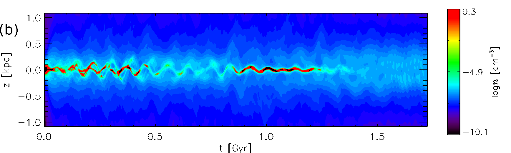
Figure C.1: Time evolution (a) of horizontal averages of gas density for Model ${\mathrm{B}2\rm{\Omega}}$ with vertical distribution of Type CC SN from $Z\sim N(0,h_{\mathrm{II}}^{2})$, and (b) with vertical distribution of Type CC SN from $Z\sim N(z_{h},h_{\mathrm{II}}^{2})$, where $z_{h}$ corresponds to the horizontal location with the largest total mass at the time of the SN explosion.

A new problem emerges with this method, however. There is a tendency for oscillations in the disc to be amplified over time, if the vertical distribution is fixed to vary about $z=0\,{\rm kpc}$. This is an unphysical effect, because one would expect the location of SNe in general to follow the star forming regions if they stray from the mid-plane. This might be overlooked for the rather shorter duration hydrodynamic simulations, but when it becomes necessary to extend runs beyond $1\,{\rm Gyr}$ to trace the dynamo, this effect not only interferes with the physical integrity of the models, it actually leads to the bulk of the gas being blown out of the model, and the simulation crashing. In Fig C.1a the horizontal averages for density from Model ${\mathrm{B}1\rm{\Omega}}$ are plotted against time. It can be seen that the disc oscillates from early on. This is natural, as intermittently one would expect the distribution of SNe to be greater above or below the disc. It is not natural, however, that the periodicity of the oscillations should be so regular nor should the amplitude be amplified. From panel (a) the initial oscillations are somewhat chaotic, and the disc fragments, with several strands of dense gas out of phase. From about 500 Myr the fragments align and the bulk of the disk mass oscillates with period $\sim 200\,{\rm Myr}$, and the displacement grows to as much as $500\,{\rm pc}$ by $1.2\,{\rm Gyr}$.

This is corrected by tracking the vertical position of the peak horizontal average gas density and adjusting the location of the SN distribution to match. To be explicit, if the horizontal slice with the highest gas density is located at $z=z_{h}$ when a Type CC SN site is being selected, then the vertical location of the site will be selected from an $N(z_{h},h_{II})$ random distribution, rather than as previously $N(0,h_{II})$. In fig. C.1b the simulation has been restarted from about 600 Myr with the revised vertical distribution. Because the SNe are now distributed symmetrically about the disc mass, the systematic oscillations are damped within 300 Myr. The perturbations to the position of the disc are more natural and are no longer unstable. In the latter stages, beyond 1.2 Gyr, the disc density distribution broadens, but this is due to the saturation of the magnetic field and the additional magnetic pressure supporting the gas against gravity.

Appendix D Dimensional units

Mee (2007, Appendix C) outlines how the system of dimensionless units for a simulation using the Pencil-code are uniquely specified by the definition of a set of fundamental units in the centimetres, grams and seconds (cgs) system. Here I clarify how these are specified, which units are currently actually defined in the code and the relation to the derived units.

The base units are length, speed and density, which are listed in Table D.1. It is desirable in numerical modelling to satisfy the constraint of finite precision that variables should not differ greatly from unity. By specifying two from three units of length, time and speed, the third unit follows. The selection of Myr or Gyr for time are natural, and with a gas speed in the ISM typically measured in $\,{\rm km\,s^{-1}}$, it follows that unit length should be of order pc or kpc, respectively.

Because $1\,{\rm Gyr}=3.15570\times 10^{16}\,{\rm s}$ and $1\,{\rm kpc}=3.08573\times 10^{31}\,{\rm cm}$, to use unit speed as $10^{5}\,{\rm km\,s^{-1}}$ I choose to approximate unit length $=3.15570\times 10^{21}\,{\rm cm}\approx 1\,{\rm kpc}$. The mean number density of atomic hydrogen near the mid-plane of the Galaxy is estimated to be about $1\,{\rm cm^{-3}}$. With the proton mass about $1.6728\times 10^{-24}\,{\rm g}$, unit density $=10^{-24}\,{\rm g}\,{\rm cm}^{-3}$ is a convenient base unit to use.

Table D.1: Specified units

Quantity	Symbol	Unit
Length	$[L]$	$3.15570\times 10^{21}\,{\rm cm}\approx 1\,{\rm kpc}$
Velocity	$[u]$	$10^{5}\,{\rm cm}\,{\rm s}^{-1}=1\,{\rm km\,s^{-1}}$
Density	$[\rho]$	$1\times 10^{-24}\,{\rm g}\,{\rm cm^{-3}}$

It is also possible to define separately units for temperature and magnetic field strength, but one should be aware that specifying a value which conflicts with the three fundamental units may lead to code instability or numerical errors. These options are necessary, to permit specification where models neglect physics such as density or velocity, but it is important to be aware that no more than three fundamental units may be specified independently, so the derived determination for magnetic field strength and temperature is required and not an arbitrary choice.

Some of the main derived units referred to in this thesis and their construction in terms of the fundamental units are listed in Table D.2. Because it is less evident how the unit of temperature and magnetic field are dependent on the specification of the fundamental units, their derivation is described explicitly below.

Table D.2: Derived units

Quantity	Symbol	Typical Derivation	Unit
Time	$[t]$	$[L][u]^{-1}$	$3.15570\times 10^{16}\,{\rm s}=1\,{\rm Gyr}$
Temperature	$[T]$	$\mu[u]^{2}\gamma^{-1}R^{-1}$	$44.74127\,{\rm K}$
Mass	$[m]$	$[\rho][L]^{3}$	$3.14256\times 10^{40}\,{\rm g}$
Energy	$[E]$	$[\rho][L]^{3}[u]^{2}$	$3.14256\times 10^{50}\,{\rm erg}$
Energy density	$[e_{V}]$	$[\rho][u]^{2}$	$1\times 10^{-14}\,{\rm erg}\,{\rm cm^{-3}}$
Pressure	$[p]$	$[\rho][u]^{2}$	$1\times 10^{-14}\,{\rm dyn}\,{\rm cm}^{-2}$
Magnetic field	$[B]$	$\sqrt{\mu_{0}}[\rho]^{\frac{1}{2}}[u]$	$3.54491\times 10^{-7}\,{\rm G}$
Kinematic viscosity	$[\nu]$	$[L][u]$	$3.15570\times 10^{26}\,{\rm erg}\,{\rm s}\,{\rm g}^{-1}$
Thermal diffusivity	$[\chi]$	$[L][u]$	$3.15570\times 10^{26}\,{\rm erg}\,{\rm s}\,{\rm g}^{-1}$
Magnetic diffusivity	$[\eta]$	$[L][u]$	$3.15570\times 10^{26}\,{\rm erg}\,{\rm s}\,{\rm g}^{-1}$
Specific entropy	$[s]$	$[u]^{2}[T]^{-1}$	$2.23507\times 10^{8}\,{\rm erg}\,{\rm g}^{-1}\,{\rm K}^{-1}$

Unit temperature and ionization

In cgs units the Boltzmann constant $k_{\textrm{B}}\simeq 1.38\times 10^{-16}\,{\rm erg}\,{\rm K}^{-1}$ and the atomic mass unit $m_{u}=1.66\times 10^{-24}\,{\rm g}$. From the equation of state

$$c{{}_{\mathrm{s}}}^{2}=\gamma\frac{p}{\rho}=\gamma\frac{k_{\textrm{B}}}{m_{u}\mu}T,$$

where the Boltzmann constant $k_{\textrm{B}}=1.380658\times 10^{-16}\,{\rm erg}\,{\rm K}^{-1}$, the atomic mass unit $m_{u}=1.6605402\times 10^{-24}\,{\rm g}$, the ratio of specific heats $\gamma=5/3$ and the mean molecular weight $\mu=0.62$. Hence unit temperature $T_{0}$ is derived from the unit sound speed $c{{}_{\mathrm{s}}}_{0}$, which is $1\,{\rm km\,s^{-1}}$, as

$$T_{0}=\frac{\mu}{\gamma R}c{{}_{\mathrm{s}}}_{0}^{2}=44.74127\,{\rm K},$$

where the gas constant $R=k_{\textrm{B}}/m_{u}$.

As is discussed in Section 3.1 in relation to Eq. 3.1 the mean molecular weight $\mu$ depends on the degree of ionization of the gas, due to the presence of free electrons. It could also depend on the presence of molecular hydrogen, but as concluded for these models, this is not resolved, so only the atomic particles contribute to $\mu$.

Assuming the gas to be fully ionized then we would have one each of hydrogen ions and electrons for each atom and for each helium atom one ion and two electrons. If $X$ is the proportion of the number of hydrogen atoms and $Y$ the proportion of helium atoms, then the total number of particles in the ISM, comprised purely of these two elements is given by

$$N= \frac{X_{i}\rho}{m_{p}}+\frac{X_{e}\rho}{m_{p}}+\frac{Y_{i}\rho}{4m_{p}}+\frac{2Y_{e}\rho}{4m_{p}}$$

$$= \frac{\rho}{m_{p}}\left(\frac{4X_{i}+4X_{e}+Y_{i}+2Y_{e}}{4}\right)$$

$$\mu^{-1}= \left(\frac{8X+3(1-X)}{4}\right)=\left(\frac{5X+3}{4}\right).$$

Given the estimates $X=0.908$ and $Y=0.092$ stated in Section 1.2.2 then for the fully ionized gas $\mu=0.531$. For the fully neutral gas, with $X_{e}=Y_{e}=0$ then $\mu=1.074$. It may be reasonable to approximate the cold gas as neutral and the hot gas as fully ionized, and to apply an appropriate temperature dependent transition between them in the warm gas, without all the additional complexity of modelling ions and electrons. Care would then need to be taken to ensure the unit of temperature is appropriate to the value of $\mu=0.531$.

Unit magnetic field strength

Similarly, in cgs units magnetic field energy density is defined as $B^{2}/(2\mu_{0})$ where the magnetic field is specified in Gauss $[\,{\rm G}]$ and the magnetic vacuum permeability $\mu_{0}=4\upi\,{\rm G}^{2}\,{\rm cm}^{3}\,{\rm erg}^{-1}$. The factor of one half is required for parity with the formulation of the thermal and kinetic energy densities. So $1\,{\rm G}=(\mu_{0}\,{\rm erg}\,{\rm cm^{-3}})^{\frac{1}{2}}$.

References

- (1)
- Balbus and Hawley (1991) Balbus, S. A. and J. F. Hawley. 1991. “A powerful local shear instability in weakly magnetized disks. I - Linear analysis. II - Nonlinear evolution.” ApJ 376:214–233.
- Balsara and Kim (2005) Balsara, D. S. and J. Kim. 2005. “Amplification of Interstellar Magnetic Fields and Turbulent Mixing by Supernova-driven Turbulence. II. The Role of Dynamical Chaos.” ApJ 634:390–406.
- Balsara et al. (2004) Balsara, D. S., J. Kim, M.-M. Mac Low and G. J. Mathews. 2004. “Amplification of Interstellar Magnetic Fields by Supernova-driven Turbulence.” ApJ 617:339–349.
- Beck et al. (1996) Beck, R., A. Brandenburg, D. Moss, A. Shukurov and D. Sokoloff. 1996. “Galactic Magnetism: Recent Developments and Perspectives.” ARA&A 34:155–206.
- Berkhuijsen and Fletcher (2008) Berkhuijsen, E. M. and A. Fletcher. 2008. “Density probability distribution functions of diffuse gas in the Milky Way.” MNRAS 390:L19–L23.
- Berkhuijsen and Fletcher (2012) Berkhuijsen, E. M. and A. Fletcher. 2012. Density PDFs of diffuse gas in the Milky Way. In EAS Publications Series, ed. M. A. de Avillez. Vol. 56 of EAS Publications Series pp. 243–246.