The Buckling of Single-Layer MoS₂ Under Uniaxial Compression

Abstract

Molecular dynamics simulations are performed to investigate the buckling of single-layer MoS₂ under uniaxial compression. The strain rate is found to play an important role on the critical buckling strain, where higher strain rate leads to larger critical strain. The critical strain is almost temperature-independent for $T<50$ K, and it increases with increasing temperature for $T>50$ K owning to the thermal vibration assisted healing mechanism on the buckling deformation. The length-dependence of the critical strain from our simulations is in good agreement with the prediction of the Euler buckling theory.

I Introduction

Molybdenum Disulphide (MoS₂) is a semiconductor with a bulk bandgap above 1.2 eV,Kam and Parkinson (1982) which can be further manipulated by changing its thickness,Mak et al. (2010) or through application of mechanical strain.Feng et al. (2012); Lu et al. (2012); Conley et al. (2013); Cheiwchanchamnangij et al. (2013a) This finite bandgap is a key reason for the excitement surrounding MoS₂ as compared to graphene as graphene has a zero bandgap.Novoselov et al. (2005); Castro Neto et al. (2009); Pereira and Castro Neto (2009) Because of its direct bandgap and also its well-known properties as a lubricant, MoS₂ has attracted considerable attention in recent years.Wang et al. (2012); Chhowalla et al. (2013) For example, Radisavljevic et al.Radisavljevic et al. (2011) demonstrated the application of single-layer MoS₂ (SLMoS₂) as a good transistor. The strain and the electronic noise effects were found to be important for the SLMoS₂ transistor.Conley et al. (2013); Sangwan et al. (2013); Ghorbani-Asl et al. (2013); Cheiwchanchamnangij et al. (2013b)

Besides the electronic properties, several recent works have addressed the thermal and mechanical properties of SLMoS₂Castellanos-Gomez et al. (2012a, b); Huang, Da, and Liang (2013); Bertolazzi, Brivio, and Kis (2011); Cooper et al. (2013a, b); Jiang, Zhuang, and Rabczuk (2013); Varshney et al. (2010); Liu et al. (2013); Castellanos-Gomez et al. (2013) Recently, we have parametrized the Stillinger-Weber potential for SLMoS₂.Jiang, Park, and Rabczuk (2013a) Based on this Stillinger-Weber potential, we derived an analytic formula for the elastic bending modulus of the SLMoS₂, where the importance of the finite thickness effect was revealed.Jiang et al. (2013) We have also shown that the MoS₂ resonator has much higher quality factor than the graphene resonator.Jiang, Park, and Rabczuk (2013b)

As an important mechanical phenomenon, the buckling of graphene has attracted lots of attention in past few years.Lu and Huang (2009); Patrick (2010); Sakhaee-Pour (2009); Pradhan and Murmu (2009); Pradhan (2009); Frank et al. (2010); Farajpour et al. (2011); Tozzini and Pellegrini (2011); Rouhi and Ansari (2012); Giannopoulos (2012); Neek-Amal and Peeters (2012); Shen, Xu, and Zhang (2013) Compared to graphene, the bending modulus of SLMoS₂ is higher by a factor of seven due to its finite thickness,Jiang et al. (2013) yet the in-plane bending stiffness in SLMoS₂ is smaller than graphene by a factor of five.Jiang, Park, and Rabczuk (2013a) As a result, the SLMoS₂ should be more difficult to be buckled than graphene, according to the Euler buckling theory, which says that the buckling critical strain is proportional to the bending modulus to in-plane stiffness ratio.Timoshenko and Woinowsky-Krieger (1987) This advantage would benefit for the application of SLMoS₂ in some mechanical devices, where the avoidance of buckling is desirable. However, the study of the buckling for the SLMoS₂ is still lacking, and is thus the focus of the present work.

In this paper, we study the buckling of the SLMoS₂ under uniaxial compression via molecular dynamics (MD) simulations. We find that the critical buckling strain increases linearly with the increase of the strain rate, and this strain rate effect becomes more important for longer SLMoS₂. The critical strain is almost temperature-independent in low-temperature regions, but it increases considerably with increasing temperature for temperatures above 50 K, because the buckling deformation is repaired by the thermal vibration at higher temperatures. We show that the critical strain depends on the length ($L$) as $\epsilon_{c}\propto 40.6/L^{2}$, which is in good agreement with the prediction of $\epsilon_{c}\propto 43.52/L^{2}$ from the Euler buckling theory.

II Euler Buckling Theory

We first present some basic knowledge for the Euler buckling theory. Similar as the visual displacement method used in Ref. Timoshenko and Woinowsky-Krieger, 1987, let’s assume that the buckling happens by exciting one normal (phonon) mode $\left(m,n\right)$ in SLMoS₂; i.e. the system is deformed into the shape corresponding to one of its normal mode,

$$w = w_{mn}=a_{mn}\sin\frac{m\pi x}{L_{x}}\sin\frac{n\pi y}{L_{y}},$$ (1)

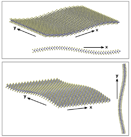
Figure 1: (Color online) The two lowest-frequency phonon normal modes in the SLMoS₂ of dimension $100\times 80$ Å, with periodic boundary condition in both $x$ and $y$ directions. The position of atom $i$ plotted in the figure is $\vec{r}_{i}=\vec{R}_{i}+C\vec{u}_{i}$, where $\vec{R}_{i}$ is the equilibrium position, $\vec{u}_{i}$ is the component of atom $i$ in the eigen vector of the normal mode. $C$ is a scaling factor for the convenience of illustration. The eigen vector is $\vec{u}_{i}=\vec{e}_{z}\sin\frac{2\pi x}{L_{x}}$ for the first lowest-frequency mode in the top panel, and $\vec{u}_{i}=\vec{e}_{z}\sin\frac{2\pi y}{L_{y}}$ for the second lowest-frequency mode in the bottom panel.

where $a_{mn}$ is the amplitude. $L_{x}$ and $L_{y}$ are the length in $x$ and $y$ directions. Integers $m$, $n=$0, 2, 4, … for periodic boundary condition. Because the buckling mode is in close relation with the normal mode, we show the first two lowest-frequency normal modes with integers $(m,n)=$ (2,0) and (0,2) in the top and bottom panels in Fig. 1. The periodic boundary condition is applied in $x$ and $y$ directions. The eigen vector is obtained by diagonalizing the dynamical matrix $K_{ij}=\partial^{2}V/\partial x_{i}\partial x_{j}$, which is obtained numerically by calculating the energy change after a small displacement of the $i$-th and $j$-th degrees of freedom.

After some simple algebra, we get the general strain energy corresponding to a general mode $(m,n)$ as

$$V_{S} = \frac{1}{2}\int\int\left[N_{x}\left(\frac{\partial w}{\partial x}\right)^{2}+N_{y}\left(\frac{\partial w}{\partial y}\right)^{2}+2N_{xy}\frac{\partial w}{\partial x}\frac{\partial w}{\partial y}\right]dxdy$$ (2)

$$= \frac{\pi^{2}}{8}L_{x}L_{y}N_{x}m^{2}\frac{a_{mn}^{2}}{L_{x}^{2}},$$

where $N_{x}$ is the force in the $x$ direction. The bending energy corresponding to the mode $(m,n)$ is

$$V_{D} = \frac{D}{2}\int\int\left\{\left(\frac{\partial^{2}w}{\partial x^{2}}+\frac{\partial^{2}w}{\partial y^{2}}\right)^{2}-2\left(1-\nu\right)\left[\frac{\partial^{2}w}{\partial x^{2}}\frac{\partial^{2}w}{\partial y^{2}}-\left(\frac{\partial^{2}w}{\partial x\partial y}\right)^{2}\right]\right\}dxdy$$ (3)

$$= \frac{\pi^{4}L_{x}L_{y}}{8}Da_{mn}^{2}\left[\left(\frac{m}{L_{x}}\right)^{2}+\left(\frac{n}{L_{y}}\right)^{2}\right]^{2},$$

where $\nu$ is the Poisson ratio and $D$ is the bending modulus.

Within the configuration just before buckling, the strain energy is maximum and there is no bending energy. After buckling, this maximum strain energy is fully converted into the bending energy; i.e. $V_{S}=V_{B}$. From this equation, we get the critical force for buckling

$$N_{x} = -\frac{\pi^{2}D}{L_{y}^{2}}\left(\frac{mL_{y}}{L_{x}}+\frac{n^{2}L_{x}}{mL_{y}}\right)^{2}.$$

Recall that $N_{x}=C_{11}\epsilon$ with $C_{11}$ as the in-plane stiffness, we get the critical strain for buckling,

$$\epsilon_{c} = -\frac{\pi^{2}D}{C_{11}L_{y}^{2}}\left(\frac{mL_{y}}{L_{x}}+\frac{n^{2}L_{x}}{mL_{y}}\right)^{2}.$$ (4)

Obviously, the minimum value of $\epsilon_{c}$ is chosen at $(m,n)=(2,0)$; i.e. the buckling happens by deforming the SLMoS₂ into the shape of the first lowest-frequency normal mode shown in the top panel of Fig. 1. We note that the choose of $m=2$ instead of $m=1$ here is the result of the constraint from the periodic boundary condition applied in the $x$ direction. The Stillinger-Weber potential gives a bending modulusJiang et al. (2013) $D=9.61$ eV and the in-plane tension stiffnessJiang, Park, and Rabczuk (2013a) $C_{11}=139.5$ Nm^-1 for the SLMoS₂. Using these two quantities, we get an explicit formula for the critical strain of SLMoS₂,

$$\epsilon_{c}=-\frac{4\pi^{2}D}{C_{11}L_{x}^{2}}=-\frac{43.52}{L_{x}^{2}}\equiv-\frac{43.52}{L^{2}}.$$ (5)

Hereafter, we will use $L$ to denote the length of the SLMoS₂ instead of $L_{x}$.

III Results and Discussions

After the representation of the Euler buckling theory, we are now performing MD simulations to study the buckling of SLMoS₂. All MD simulations in this work are performed using the publicly available simulation code LAMMPS Plimpton (1995); Lammps (2012), while the OVITO package was used for visualization in this section Stukowski (2010). The standard Newton equations of motion are integrated in time using the velocity Verlet algorithm with a time step of 1 fs. The interaction within MoS₂ is described by the Stillinger-Weber potential, where the parameters for this potential have been fitted to the phonon dispersion of single-layer and bulk MoS₂.Jiang, Park, and Rabczuk (2013a) The phonon dispersion is closely related to some mechanical quantities like Young’s modulus and some thermal properties, so this parameter set can give a good description for the mechanical and thermal properties of the single-layer MoS₂. Periodic boundary conditions are applied in the two in-plane directions, and the free boundary condition is applied in the out-of-plane direction. Our simulations are performed as follows. First, the Nosé-HooverNose (1984); Hoover (1985) thermostat is applied to thermalize the system to a constant pressure of 0, and a constant temperature of 1.0 K within the NPT (i.e. the particles number N, the pressure P and the temperature T of the system are constant) ensemble, which is run for 100 ps. The SLMoS₂ is then compressed in the x-direction within the NPT ensemble, which is also maintained through the Nosé-Hoover thermostat. The SLMoS₂ is compressed unaxially along the $x$ direction by uniformly deforming the simulation box in this direction, while it is allowed to be fully relaxed in lateral directions during the compression.

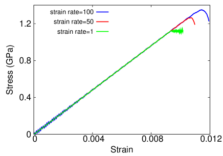
Figure 2: (Color online) Stress strain relation under compression for SLMoS₂ with length 60 Å and width 40 Å at 1.0 K. The curve drops sharply at a critical strain $\epsilon_{c}=0.00939$ when the SLMoS₂ is compressed at a strain rate $\dot{\epsilon}=1.0$ $\mu$s^-1.

We shall examine the strain rate effect on the critical strain. Fig. 2 shows the stress strain relation under compression for SLMoS₂ with length 60 Å and width 40 Å at 1.0 K low temperature. The buckling phenomenon happens when the SLMoS₂ is compressed with the critical strain $\epsilon_{c}$, which corresponds to a sharp drop in the curve. The critical strain $\epsilon_{c}=0.00939$, 0.01073, and 0.01141 correspond to the strain rate of $\dot{\epsilon}=1.0$ $\mu$s^-1, 10.0 $\mu$s^-1, and 100.0 $\mu$s^-1. The critical strain increases with increasing strain rate. It is because the system is compressed so fast that the relaxation time is not long enough for the occurrence of the buckling phenomenon.

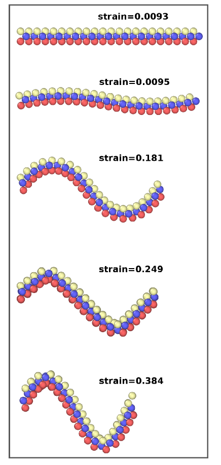
Figure 3: (Color online) The structure evolution for SLMoS₂ with length 60 Å and width 40 Å at 1.0 K. The SLMoS₂ is compressed at a strain rate $\dot{\epsilon}=1.0$ $\mu$s^-1. The buckling happens at $\epsilon=0.00939$. The structure transforms from sinuous into zigzag at $\epsilon=0.249$.

Fig. 3 shows the configuration evolution for the SLMoS₂. The SLMoS₂ is compressed at a strain rate $\dot{\epsilon}=1.0$ $\mu$s^-1. The buckling happens at $\epsilon=0.00939$. The first normal mode buckling is observed at the critical strain, as this mode has the lowest exciting energy. The figure shows that MoS₂ is further deformed with more strain applied. However, the deformation always follows the shape of the first normal mode, and no high-order normal mode is observed. It indicates that the strain energy stored in the buckled SLMoS₂ (with first normal mode buckling) is not large enough to jump from the first normal mode to high-order normal mode. It is because this jumping requires the reverse of a ripple (with large bending curvature) in the first normal mode, which is forbidden by high potential threshold. It is quite interesting that the structure transforms from sinuous into zigzag at $\epsilon=0.249$, due to stress concentration at the two valleys of the sinuous shape.

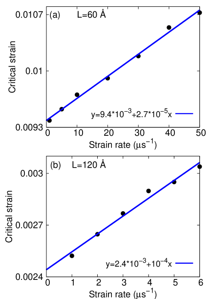
Figure 4: (Color online) The strain rate effect on the critical strain for SLMoS₂ with width 40 Å at 1.0 K. The critical strain increases linearly with increasing strain rate for SLMoS₂ with length $L=60$ Å in (a) and $L=120$ Å in (b). Note that the slope ($2.7\times 10^{-5}$ $\mu$s) of the fitting line in the shorter system in (a) is only a quarter of the slope of $1.0\times 10^{-4}$ $\mu$s in the longer MoS₂ in (b), which implies that the strain rate has stronger effect for longer MoS₂.

To further examine the strain rate effect on the critical strain, we perform systematic simulations for the buckling of the SLMoS₂ under compression with different strain rate. Fig. 4 shows the critical strain for SLMoS₂ with width 40 Å at 1.0 K. The length of the SLMoS₂ is 60 Å in panel (a) and 120 Å in panel (b). In both systems, the critical strain increases linearly with increasing strain rate. The simulation data are fitted to a linear function $y=a+bx$, where the coefficient $a=9.4\times 10^{-3}$ and $2.4\times 10^{-3}$ can be regarded as the exact value (with $\dot{\epsilon}\rightarrow 0.0$) for the critical strain in these two SLMoS₂. Using a strain rate of 1.0 $\mu$s^-1, we get the critical strains 0.00938 and 0.00252 for SLMoS₂ with $L=60$ Å and 120 Å. As a result, the error due to using a finite strain rate of 1.0 $\mu$s^-1 is 0.2% and 5% for these two SLMoS₂. For the coefficient $b$, this slope of the fitting line in the shorter system in panel (a) is $2.7\times 10^{-5}$ $\mu$s, which is only a quarter of the slope of $1.0\times 10^{-4}$ $\mu$s in the longer MoS₂ in panel (b). It indicates that the strain rate has stronger effect for longer SLMoS₂, because the frequency of the buckling mode (first lowest-frequency normal mode) is lower in longer system, leading to longer response time. That is the buckling mode in a longer SLMoS₂ requires longer relaxation time for its occurrence.

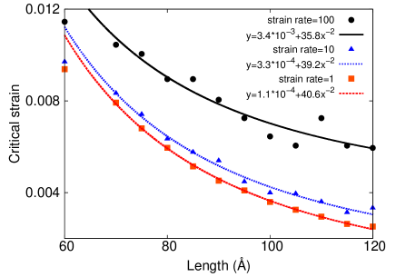
Figure 5: (Color online) The length dependence of the critical strain in SLMoS₂ with width 40 Å at 1.0 K. The system is compressed at the strain rate of 1.0 $\mu$s^-1 (red squares), 10.0 $\mu$s^-1 (blue triangles), and 100.0 $\mu$s^-1 (black circles). Lines are the fitting to function $y=a+bx^{-2}$, where the coefficient $b$ increases with increasing strain rate. In particular, the coefficient of $b=40.6$ Å² for $\dot{\epsilon}=1.0$ $\mu$s^-1 is only 6.7% smaller than the prediction from the Euler buckling theory of $b=4\pi^{2}D/C_{11}=43.52$ Å², where $D$ is the bending modulus and $C_{11}$ is the in-plane stiffness for SLMoS₂.

Fig. 5 shows the length dependence of the critical strain in SLMoS₂ with width 40 Å. This set of simulations are performed at a low temperature of 1.0 K, so that it can be consistent with the static Euler buckling theory. The system is compressed at the strain rate of 1.0 $\mu$s^-1 (red squares), 10.0 $\mu$s^-1 (blue triangles), and 100.0 $\mu$s^-1 (black circles). According to the Euler buckling theory, the critical strain is inversely proportional to the square of the length of the SLMoS₂, so we fit simulation data to function $y=a+bx^{-2}$. The coefficient $b$ increases with increasing strain rate. In particular, the coefficient of $b=40.6$ Å² for $\dot{\epsilon}=1.0$ $\mu$s^-1 agrees quite well with (error 6.7%) the prediction from the Euler buckling theory of $b=4\pi^{2}D/C_{11}=43.52$ Å², where $D$ is the bending modulus and $C_{11}$ is the in-plane stiffness for SLMoS₂. Furthermore, for the strain rate $\dot{\epsilon}=1.0$ $\mu$s^-1, the other coefficient $a$ is pretty small and there is almost no fluctuation between simulation data, both of which validate the usage of the small strain rate, $\dot{\epsilon}=1.0$ $\mu$s^-1. The critical strain for the shortest SLMoS₂ ($L=60$ Å) deviates from the fitting curve in all of the three situations. It is due to the linear nature of the Euler buckling theory, while the nonlinear effect becomes important in the short system. The critical strain does not depend on the width of the SLMoS₂, because the shape of the buckling mode is uniform in the width direction. Hence, the strain energy is the same in SLMoS₂ of different widths. That is why the width parameter does not present in the Euler buckling formula Eq. (5).

Fig. 6 shows the temperature effect on the critical strain for SLMoS₂ with width 40 Å at strain rate 1.0 $\mu$s^-1. Panel (a) is the temperature dependence of the relative critical strain versus for SLMoS₂ with $L=60$ and 120 Å. The relative critical strain is scaled by the value at 1.0 K; i.e. 0.00939 and 0.00252 for $L=60$ and 120 Å respectively. Lines are guided to the eye. The critical strain in both systems keeps almost a constant at temperatures bellow 50 K. It increases linearly with increasing temperature for temperatures above 50 K, and the critical strain increases faster in longer SLMoS₂. This is due to strong thermal vibration at high temperatures. Panel (b) shows the maximum thermal vibration amplitude versus temperature for SLMoS₂ with $L=60$ (black circles) and 120 Å (red squares). According to the equipartition theorem, the maximum thermal vibration amplitude can be fitted to function $y=ax^{0.5}$. Lines are the fitting results. The maximum vibration amplitude increases with increasing temperature. At higher temperatures (above 50 K), the maximum vibration amplitude is so large that it can disturb the buckling mode; i.e. the strong thermal vibration is able to heal the buckling-induced deformation in the SLMoS₂. At the initial buckling stage, atoms are displaced from its original position (following the buckling mode, i.e first lowest-frequency normal mode), but atoms are involved in a strong thermal vibration in the mean time. This large thermal vibration amplitude blurs the buckling deformation and the original configuration of the SLMoS₂. In other words, the thermal vibration introduces a healing mechanism for the buckling deformation at the initial buckling stage. Similar thermal healing mechanism has also been observed in the thermal treatment for defected carbon materials.Kim et al. (2004); Jiang and Wang (2010) Hence, larger compression strain is in need to intrigue the buckling phenomenon at higher temperatures.

We end by noting that the present atomistic simulation actually has practical impact, although we emphasized the importance of the strain rate and temperature effects on the buckling of the SLMoS₂, which are technique aspects. MoS₂ and graphene have complementary physical properties, so it is natural to investigate the possibility of combining graphene and MoS₂ in specific ways to create heterostructures that mitigate the negative properties of each individual constituent. For example, graphene/MoS₂/graphene heterostructures have better photon absorption and electron-hole creation properties, because of the enhanced light-matter interactions by the single-layer MoS₂.Britnell et al. (2013) It has been shown that the buckling critical strain for a graphene of 19.7 Å in length is around 0.0068.Lu and Huang (2009) From Euler buckling theorem, it can be extracted that the buckling critical strain for a graphene of 60.0 Å in length is around 0.00073. Our simulations have shown that the buckling critical strain for SLMoS₂ of the same length is 0.0094, which is one order higher than graphene. It indicates that the SLMoS₂ can sustain stronger compression than graphene. The higher buckling critical strain for the SLMoS₂ is helpful for the graphene/MoS₂ heterostructure to protect from buckling damage.

IV Conclusion

In conclusion, we have performed MD simulations to investigate the buckling of the SLMoS₂ under uniaxial compression. In particular, we examine the importance of the strain rate and temperature effects on the critical buckling strain. The critical strain increases linearly with increasing strain rate, and it keeps almost a constant at low temperatures. The critical strain increases with increasing temperature at temperatures above 50 K, because the strong thermal vibration is able to repair the buckling-induced deformation. The length dependence for the critical strain is in good agreement with the Euler buckling theory.

Acknowledgements The work is supported by the Recruitment Program of Global Youth Experts of China and the start-up funding from the Shanghai University.

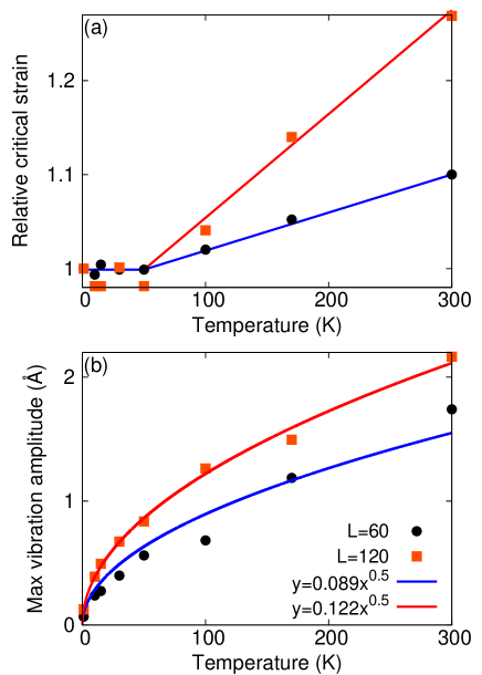
Figure 6: (Color online) The temperature effect on the critical strain for SLMoS₂ with width 40 Å at strain rate 1.0 $\mu$s^-1. (a) Relative critical strain versus temperature for SLMoS₂ with $L=60$ and 120 Å. The relative critical strain is scaled by the value at 1.0 K; i.e. 0.00939 and 0.00252 for $L=60$ and 120 Å respectively. Lines are guided to the eye. (b) The maximum thermal vibration amplitude versus temperature for SLMoS₂ with $L=60$ (black circles) and 120 Å (red squares). Lines are fitting to function $y=ax^{0.5}$.

References

- Kam and Parkinson (1982) K. K. Kam and B. A. Parkinson, Journal of Physical Chemistry 86, 463 (1982).
- Mak et al. (2010) K. F. Mak, C. Lee, J. Hone, J. Shan, and T. F. Heinz, Physical Review Letters 105, 136805 (2010).
- Feng et al. (2012) J. Feng, X. Qian, C. . Huang, and J. Li, Nature Photonics 6, 866 (2012).
- Lu et al. (2012) P. Lu, X. Wu, W. Guo, and X. C. Zeng, Phys. Chem. Chem. Phys. 14, 13035 (2012).
- Conley et al. (2013) H. J. Conley, B. Wang, J. I. Ziegler, R. F. Haglund, S. T. Pantelides, and K. I. Bolotin, Nano Letters 13, 3626 (2013).
- Cheiwchanchamnangij et al. (2013a) T. Cheiwchanchamnangij, W. R. L. Lambrecht, Y. Song, and H. Dery, Physical Review B 88, 155404 (2013a).
- Novoselov et al. (2005) K. S. Novoselov, A. K. Geim, S. V. Morozov, D. Jiang, M. I. Katsnelson, I. V. Grigorieva, S. V. Dubonos, and A. A. Firsov, Nature 438, 197 (2005).
- Castro Neto et al. (2009) A. H. Castro Neto, F. Guinea, N. M. R. Peres, K. S. Novoselov, and A. K. Geim, Rev. Mod. Phys. 81, 109 (2009).
- Pereira and Castro Neto (2009) V. M. Pereira and A. H. Castro Neto, Physical Review Letters 103, 046801 (2009).
- Wang et al. (2012) Q. H. Wang, K. Kalantar-Zadeh, A. Kis, J. N. Coleman, and M. S. Strano, Nature Nanotechnology 7, 699 (2012).
- Chhowalla et al. (2013) M. Chhowalla, H. S. Shin, G. Eda, L. . Li, K. P. Loh, and H. Zhang, Nature Chemistry 5, 263 (2013).
- Radisavljevic et al. (2011) B. Radisavljevic, A. Radenovic, J. Brivio, V. Giacometti, and A. Kis, Nature Nanotechnology 6, 147 (2011).
- Sangwan et al. (2013) V. K. Sangwan, H. N. Arnold, D. Jariwala, T. J. Marks, L. J. Lauhon, and M. C. Hersam, Nano Letters 13, 4351 (2013).
- Ghorbani-Asl et al. (2013) M. Ghorbani-Asl, N. Zibouche, M. Wahiduzzaman, A. F. Oliveira, A. Kuc, and T. Heine, Scientific Reports 3, 2961 (2013).
- Cheiwchanchamnangij et al. (2013b) T. Cheiwchanchamnangij, W. R. L. Lambrecht, Y. Song, and H. Dery, Physical Review B 88, 155404 (2013b).
- Huang, Da, and Liang (2013) W. Huang, H. Da, and G. Liang, Journal of Applied Physics 113, 104304 (2013).
- Jiang, Zhuang, and Rabczuk (2013) J.-W. Jiang, X.-Y. Zhuang, and T. Rabczuk, Scientific Reports 3, 2209 (2013).
- Varshney et al. (2010) V. Varshney, S. S. Patnaik, C. Muratore, A. K. Roy, A. A. Voevodin, and B. L. Farmer, Computational Materials Science 48, 101 (2010).
- Bertolazzi, Brivio, and Kis (2011) S. Bertolazzi, J. Brivio, and A. Kis, ACS Nano 5, 9703 (2011).
- Cooper et al. (2013a) R. C. Cooper, C. Lee, C. A. Marianetti, X. Wei, J. Hone, and J. W. Kysar, Physical Review B 87, 035423 (2013a).
- Cooper et al. (2013b) R. C. Cooper, C. Lee, C. A. Marianetti, X. Wei, J. Hone, and J. W. Kysar, Physical Review B 87, 079901 (2013b).
- Liu et al. (2013) X. Liu, G. Zhang, Q.-X. Pei, and Y.-W. Zhang, Applied Physics Letters 103, 133113 (2013).
- Castellanos-Gomez et al. (2012a) A. Castellanos-Gomez, M. Poot, G. A. Steele, H. S. J. van der Zant, N. Agrait, and G. Rubio-Bollinger, Advanced Materials 24, 772 (2012a).
- Castellanos-Gomez et al. (2013) A. Castellanos-Gomez, R. Roldan, E. Cappelluti, M. Buscema, F. Guinea, H. S. J. van der Zant, and G. A. Steele, Nano Letters 13, 5361 (2013).
- Castellanos-Gomez et al. (2012b) A. Castellanos-Gomez, M. Poot, G. A. Steele, H. S. J. van der Zant, N. Agraït, and G. Rubio-Bollinger, Nanoscale Res Lett 7, 1 (2012b).
- Jiang, Park, and Rabczuk (2013a) J.-W. Jiang, H. S. Park, and T. Rabczuk, Journal of Applied Physics 114, 064307 (2013a).
- Jiang et al. (2013) J.-W. Jiang, Z. Qi, H. S. Park, and T. Rabczuk, Nanotechnology 24, 435705 (2013).
- Jiang, Park, and Rabczuk (2013b) J.-W. Jiang, H. S. Park, and T. Rabczuk, Nanoscale 6, 3618 (2013b).
- Lu and Huang (2009) Q. Lu and R. Huang, International Journal of Applied Mechanics 1, 443 (2009).
- Patrick (2010) W. J. Patrick, Journal of Computational and Theoretical Nanoscience 7, 2338 (2010).
- Sakhaee-Pour (2009) A. Sakhaee-Pour, Computational Materials Science 45, 266 (2009).
- Pradhan and Murmu (2009) S. C. Pradhan and T. Murmu, Computational Materials Science 47, 268 (2009).
- Pradhan (2009) S. C. Pradhan, Physics Letters, Section A: General, Atomic and Solid State Physics 373, 4182 (2009).
- Frank et al. (2010) O. Frank, G. Tsoukleri, J. Parthenios, K. Papagelis, I. Riaz, R. Jalil, K. S. Novoselov, and C. Galiotis, ACS Nano 4, 3131 (2010).
- Farajpour et al. (2011) A. Farajpour, M. Mohammadi, A. R. Shahidi, and M. Mahzoon, Physica E: Low-dimensional Systems and Nanostructures 43, 1820 (2011).
- Tozzini and Pellegrini (2011) V. Tozzini and V. Pellegrini, Journal of Physical Chemistry C 115, 25523 (2011).
- Rouhi and Ansari (2012) S. Rouhi and R. Ansari, Physica E: Low-dimensional Systems and Nanostructures 44, 764 (2012).
- Giannopoulos (2012) G. I. Giannopoulos, Computational Materials Science 53, 388 (2012).
- Neek-Amal and Peeters (2012) M. Neek-Amal and F. M. Peeters, Applied Physics Letters 100, 101905 (2012).
- Shen, Xu, and Zhang (2013) H. . Shen, Y. . Xu, and C. . Zhang, Applied Physics Letters 102, 131905 (2013).
- Timoshenko and Woinowsky-Krieger (1987) S. Timoshenko and S. Woinowsky-Krieger, Theory of Plates and Shells, 2nd ed (McGraw-Hill, New York, 1987).
- Plimpton (1995) S. J. Plimpton, Journal of Computational Physics 117, 1 (1995).
- Lammps (2012) Lammps, http://www.cs.sandia.gov/sjplimp/lammps.html (2012).
- Stukowski (2010) A. Stukowski, Modelling and Simulation in Materials Science and Engineering 18, 015012 (2010).
- Nose (1984) S. Nose, Journal of Chemical Physics 81, 511 (1984).
- Hoover (1985) W. G. Hoover, Physical Review A 31, 1695 (1985).
- Kim et al. (2004) Y. A. Kim, H. Muramatsu, T. Hayashi, M. Endo, M. Terrones, and M. S. Dresselhaus, Chemical Physics Letters 398, 87 (2004).
- Jiang and Wang (2010) J.-W. Jiang and J.-S. Wang, Journal of Applied Physics 108, 054303 (2010).
- Britnell et al. (2013) L. Britnell, R. M. Ribeiro, A. Eckmann, R. Jalil, B. D. Belle, A. Mishchenko, Y.-J. Kim, R. V. Gorbachev, T. Georgiou, S. V. Morozov, A. N. Grigorenko, A. K. Geim, C. Casiraghi, A. H. C. Neto, and K. S. Novoselov, Science 340, 1311 (2013).