Solar modulations by the regular
heliospheric electromagnetic field

Abstract

The standard way to model the cosmic ray solar modulations is via the Parker equation, that is as the effect of diffusion in the turbulent magnetic of an expanding solar wind. Calculations performed with this method that do not include a description of the regular magnetic field in the heliosphere predict, in disagreement with the observations, equal modulations for particles and antiparticles. The effects of the regular heliospheric field, that break the the particle/anti–particle symmetry, have been included in the Parker equation adding convection terms associated to the magnetic drift velocity of charged particles moving in non–homogeneous magnetic field. In this work we take a completely different approach and study the propagation of charged particles in the heliosphere assuming only the presence of the regular magnetic field, and completely neglecting the random component. Assuming that the field is purely magnetic in the wind frame, one can deduce the existence of a large scale electric field, that results in important energy losses for charged particles that traverse the heliosphere and reach the Earth. The energy loss $\Delta E$ due to the large scale regular electric field depends on the particle electric charge, is proportional to the absolute value of the electric charge, and to a good approximation is independent from the particle energy and direction. We speculate that this deterministic energy loss is an important, or perhaps even the leading contribution to the solar modulation effects.

1 Introduction

The fluxes of galactic cosmic rays observed near the Earth are different from those present in the local interstellar space because the particles lose energy and are deviated when they penetrate the heliosphere. These effects are time dependent because the heliospheric environment is not static. The time variations have several different characteristic time scales with a prominent 22 years periodicity associated to the solar magnetic activity. The solar modulations of the cosmic rays energy spectra have been extensively studied experimentally for many years using ground and space based detectors, and has been the subject of many theoretical studies [1].

Following the pioneering work of Parker [2], the usual way to study theoretically the solar modulations is to model the propagation of cosmic rays in the heliosphere as a diffusion process in a turbulent magnetic field, accompanied by convection (because of the motions of the plasma – the solar wind – that fills the heliosphere) and adiabatic energy losses associated to the expansion of the plasma. The effects of diffusion, convection and adiabatic energy loss in particle propagation are included in the Parker equation that has been used as the standard instrument to study solar modulations (for a recent reviews see [4]).

In the first studies of the solar modulations (such as [3]) the calculated effects were identical for particles of opposite electric charge. The data however show that the modulations effects differ for particles of opposite electric charge. The dependence of the modulations on the sign of the electric charge can be attributed to the presence of a regular magnetic field in the heliosphere. In the presence of such a field, the average trajectories of particles with opposite charge differ, and the particles can have different energy losses.

The effects of the regular heliospheric field was first included in the Parker equation by Jokipii [5] introducing an additional convection term associated to the average “drift velocity” of the gyration center of charged particles moving in a non–homogeneous magnetic field. The direction of the drift velocity is reversed when the electric charge of a particle changes sign, and therefore the drift velocity convection term breaks the particle/antiparticle symmetry in the Parker equation [6, 7, 8].

In this work we will discuss the propagation of charged particles in the heliosphere assuming that only the regular electromagnetic field is present, neglecting completely the effects of the random component of the field. This approach is complementary to the traditional method (where it is the regular field that is completely neglected), and a comparison of the results can be instructive to clarify the physical mechanisms that generate the solar modulations.

To keep the discussion as simple as possible we will assume that the heliospheric magnetic field $\vec{\boldsymbol{B}}(\vec{x})$ has the simple Parker spiral form (discussed below), and that the speed of the solar wind is constant, and its direction is radial ($\vec{w}(\vec{x})=w\,\hat{r}$). The magnetic field and the solar wind will be also considered as stationary during the time necessary for charged particles to reach the Earth from the boundary of the heliosphere.

If the conductivity of the plasma in the heliosphere is sufficiently high, the condition of stationarity implies that the net force on an electrically charged particle moving with the wind must vanish. It follows that in a frame where the Sun is at rest there is a non vanishing electric field given by the well known expression:

$$\vec{\boldsymbol{E}}(\vec{x})=-\frac{\vec{w}(\vec{x})}{c}\wedge\vec{\boldsymbol{B}}(\vec{x})~{}.$$ (1)

Equation (1) can be also derived requiring that the electric field vanishes in a frame where the plasma of the solar wind is at rest.

Under the assumptions we have outlined above, the propagation of a charged particle in the heliosphere, is completely deterministic and can be calculated integrating the classical equations of motion:

$$\frac{d\vec{x}}{dt}=\vec{v}=\frac{\vec{p}}{\sqrt{p^{2}+m^{2}}}$$ (2)

$$\frac{d\vec{p}}{dt}=q\;\left(\vec{\boldsymbol{E}}+\frac{\vec{v}}{c}\wedge\vec{\boldsymbol{B}}\right)~{}.$$

In the following we will show that charged particles of sufficiently low energy ($E\lesssim 1$ TeV) propagating from the boundary of the heliosphere to the Earth will always lose energy, and discuss the properties and consequences of this energy loss.

This paper is organized as follows: in the next section we describe the model of the heliospheric electromagnetic fields used in this work. In section 3 we discuss the magnetic drift velocities in the motion of charged particles in our heliospheric model. In section 4 we discuss some examples of trajectories of charged particles in the heliosphere. Section 5 discusses the energy loss suffered by particles that arrive at the Earth. Section 6 discusses the relation between the interstellar spectra of cosmic rays at the boundary of the heliosphere, and the energy spectra observable at the Earth. The last section gives a summary and outlook.

2 Electromagnetic fields in the heliosphere

In the following we will assume that the solar magnetic field has the Parker spiral form:

$$\vec{\boldsymbol{B}}=A~{}B_{0}\;\left(\frac{r_{0}}{r}\right)^{2}\;\left[\hat{r}-\frac{\Omega}{w}\,r\,\sin\theta\;\hat{\varphi}\right]\;S(\vec{r})$$ (3)

In this equation $r$, $\theta$ and $\varphi$ are spherical coordinates in a frame centered on the Sun, $\hat{r}$ and $\hat{\varphi}$ are versors, $r_{0}$ is the radius of the Earth orbit (approximated as a circle), $\Omega$ is the (equatorial) frequency of the solar rotation, $w$ is the speed of the solar wind that we will assume is radial and constant ($\vec{w}=w\;\hat{r}$), $B_{0}$ is a normalization constant, $A=\pm 1$ give the polarity of the solar cycle (that is reversed approximately every 11 years), and $S(\vec{r})$ is $\pm 1$:

$$S(\vec{r})=\begin{cases}+1&\mbox{if }\cos\theta>\cos\theta^{*}\\ -1&\mbox{if }\cos\theta\leq\cos\theta^{*}\end{cases}$$ (4)

with

$$\cos\theta^{*}=-\sin\alpha\,\sin\left(\varphi+\frac{\Omega}{w}\,r\right)~{}.$$ (5)

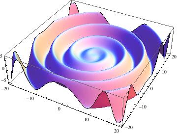
Figure 1: Representation of the heliospheric current sheet for tilt angle $\sin\alpha=0.2$.

The set of points that satisfy the equation $\cos\theta=\cos\theta^{*}$ forms a surface known as the Heliospheric Current Sheet (HCS) where the magnetic field is discontinuous. The “tilt angle” $\alpha$ can take values in the interval $[0,\pi/2]$. For $\alpha=0$ the HCS coincides with the $xy$ equatorial plane, more in general the surface has the wavy form of a “ballerina skirt”. The shape of the current sheet is illustrated in fig.1, 2 and 3.

It is convenient to introduce the characteristic length:

$$R=\frac{w}{\Omega}\simeq 0.93~{}\left[\frac{w}{400~{}{\rm km/s}}\right]{\rm AU}\;,$$ (6)

that will enter in several expressions in the following. The modulus of the magnetic field is:

$$\left|\boldsymbol{B}\right(\vec{x})|=B_{0}\;\left(\frac{r_{0}}{r}\right)^{2}\sqrt{1+\frac{\Omega^{2}}{w^{2}}\;(r^{2}-z^{2})}~{}.$$ (7)

When $r$ increases for a fixed direction $\hat{n}$, the field decreases in general $\propto r^{-1}$, with the only exception of the $\pm\hat{z}$ directions, when the field is $\propto r^{-2}$. The field at the Earth is:

$$B_{\oplus}=B_{0}\;\sqrt{1+\left(\frac{\Omega\,r_{0}}{w}\right)^{2}}~{}.$$ (8)

The magnetic field lines have the form of clockwise Archimedes spirals that are enveloped on a cone with vertical axis and vertex at the origin of the coordinates. The field line that passes through the point with polar coordinates $\{\overline{r},\overline{\theta},\overline{\varphi}\}$ can be parametrized in terms of the azimuth angle $\varphi$ of the points along the line:

$$\theta(\varphi) = \overline{\theta}$$ (9)

$$r(\varphi) = \overline{r}+R\times\left[\overline{\varphi}-\varphi\right]$$

with the angle $\varphi$ in the interval:

$$-\infty<\varphi\leq\varphi_{\rm max}=\overline{\varphi}+\frac{\overline{r}}{R}~{}.$$ (10)

The range of variation of $\varphi$ in the previous equations shows that each field line extends to infinity in one direction and reaches the origin at $r=0$ after a finite length in the opposite direction. The distance from the origin of a point on the line grows linearly with $\varphi_{\rm max}-\varphi$, and the quantity $\varphi_{\rm max}$ gives the azimuth angle of the field line direction at the origin.

For positive polarity ($A>0$) the magnetic lines are outward (inward) in the hemisphere above (below) the heliospheric current sheet. For negative polarity ($A<0$) the direction of all field lines is reversed.

The heliospheric electric field can be calculated using equation (1). In cartesian components one has:

$$\vec{\boldsymbol{E}}(x,y,z)=\pm A\,B_{0}\;\frac{\Omega\,r_{0}^{2}}{c\,r^{3}}\left\{x\,z,y\,z,-(x^{2}+y^{2})\right\}$$ (11)

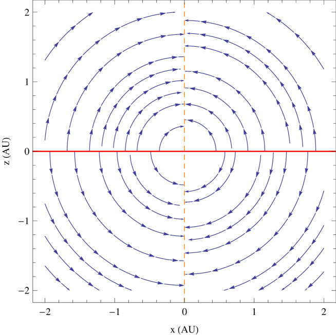
Figure 4: Streamlines of the electric field in the heliosphere. The thick line represents the heliospheric current sheet. The electric field $\vec{Ef}$ has cylindrical symmetry and vanishes along the line $x=0$. The figure is valid for $A>0$. For $A<0$ the field direction is reversed.

where the $+$ ($-$) sign applies above (below) the heliospheric current sheet. Note that the near the heliospheric equator the electric field is vertical, and points toward the HCS for $A>0$, and away from the HCS for $A<0$. The streamlines of the electric field are shown in fig.4. The modulus of the electric field is

$$\left|\vec{\boldsymbol{E}}(x,y,z)\right|=B_{0}\;\frac{\Omega\,r_{0}^{2}}{c}\;\frac{\sqrt{x^{2}+y^{2}}}{r^{2}}$$ (12)

The divergence and rotor of $\vec{\boldsymbol{E}}$ are:

$$\nabla\cdot\vec{\boldsymbol{E}}=\pm A\,B_{0}\;\frac{\Omega\,r_{0}^{2}}{c}\;\frac{2z}{r^{3}}$$ (13)

and

$$\nabla\wedge\vec{\boldsymbol{E}}=0~{}.$$ (14)

Equation (13) implies that a non vanishing electric charge density must be present in the heliosphere to satisfy the Maxwell equations. Equation (14) has very important consequences, because it implies that the electric field can be written as the gradient of a potential function:

$$\vec{\boldsymbol{E}}(x,y,z)=-\nabla V(x,y,z)~{}.$$ (15)

Choosing the constant so that the potential vanishes at the heliospheric equator $z=0$, the electric potential $V$ is:

$$V(x,y,z)=\mp A\,B_{0}\;\frac{\Omega\,r_{0}^{2}}{c}\;\frac{z}{r}~{}$$ (16)

where the $\mp$ sign is valid above (below) the heliospheric current sheet. Note that on the HCS the electric potential $V$ (as also the electric and magnetic fields) is discontinuous for all points that have $z\neq 0$. A $z=0$, when the HCS coincides with the equatorial plane, the potential vanishes and is continuous (but the electric and magnetic fields are discontinuous).

The limits of the potential for $z\pm\infty$ (with $x$ and $y$ finite) are equal to each other, and independent from the values of $x$ and $y$:

$$\lim_{z\pm\infty}V(x,y,z)=V_{\infty}=-A\,\left|V_{\infty}\right|=-A\,B_{0}\;\frac{\Omega\,r_{0}^{2}}{c}~{}.$$ (17)

Note that $V_{\infty}$, the asymptotic value of the potential for $|z|\to\infty$, changes sign with the polarity of the solar phase (is negative for $A>0$, and positive for $A<0$). The existence of the electric field potential and the result that all points with large $|z|$ have the same potential have important consequences that will be discussed later.

It should be noted that the Parker spiral expression of equation (3) cannot be a good description of the magnetic field in all space, and it must fail both for very small and very large distances from the origin of the coordinates. This can be verified computing the total energy of the magnetic field. Integrating the energy density $B^{2}/(8\pi)$ of the Parker spiral field in the volume contained between radii $r_{\rm min}$ and $r_{\rm max}$ one obtains:

$$E_{\rm magnetic}=\frac{B_{0}^{2}\,r_{0}^{4}}{2}\;\left[\frac{1}{r_{\rm min}}-\frac{1}{r_{\rm max}}+\frac{2}{3}\,\frac{(r_{\rm max}-r_{\rm min})}{(w/\Omega)^{2}}\right]~{}.$$ (18)

This expression diverges in the limits $r_{\rm min}\to 0$ and $r_{\rm max}\to\infty$ demonstrating that a Parker spiral magnetic field that extends to all space is unphysical. The extension of the Parker spiral form to $r\to\infty$ would in fact correspond to the assumption of a solar wind emitted with constant velocity for an infinitely long time in the past.

The expression (3) for the heliospheric magnetic field should therefore be considered as approximately valid only in a finite volume outside an inner spherical surface of few solar radii, and inside the termination shock, a roughly spherical surface with a radius of approximately 100 AU where the solar wind suffers an abrupt deceleration.

In this work we will not attempt to model the magnetic field outside the termination shock, that is in fact only very poorly known. The results shown here are not very sensitive to the size of the volume where the field is well described as a Parker spiral, if it extends to a radius equal or larger than $\sim 100$ AU.

3 Drift velocity

The motion of a particle in a non homogeneous magnetic field can be decomposed into the gyration around the field lines accompanied by the drift of the gyration center in a direction orthogonal to the lines [9]. The drift velocity is given by the well known expression:

$$\vec{v}_{\rm drift}=\frac{\vec{\boldsymbol{B}}\wedge\vec{\nabla}|\boldsymbol{B}|}{2\,q\,|\boldsymbol{B}|^{3}}\;E\,c\;\left(\beta_{\perp}^{2}+2\,\beta_{\parallel}^{2}\right)$$ (19)

where $q$ and $E$ are the charge and energy of the particle, and $\beta_{\perp}$ and $\beta_{\parallel}$ are the components of the particle velocity orthogonal and parallel to the magnetic field. The two terms proportional to $\beta_{\perp}^{2}$ and $\beta_{\parallel}^{2}$ are known as the gradient and curvature contributions to the drift velocity.

For a magnetic field of the Parker spiral form the drift velocity can be calculated explicitely as:

$$\vec{v}_{\rm drift}=\pm A\,\frac{q}{|q|}\,V_{\beta}\,\;\left[\hat{\rho}\;\frac{2\,\rho\,z}{R^{2}+z^{2}}+\hat{\varphi}\;\frac{R\rho z\,\sqrt{\rho^{2}+z^{2}}}{(R^{2}+z^{2})^{2}}-\hat{z}\;\frac{\rho^{2}\,(2R^{2}+\rho^{2}-z^{2})}{(R^{2}+z^{2})^{2}}\right]$$ (20)

where again the $\pm$ sign applies above (below) the heliospheric current sheet, $\hat{\rho}$, $\hat{\varphi}$ and $\hat{z}$ are versors in the three directions of cylindrical coordinates (with $\rho=\sqrt{x^{2}+y^{2}}$), the length $R$ was defined in equation (6) and $V_{\beta}$, with the dimensions of a velocity, is:

$$V_{\beta}=V_{0}~{}\left(\beta_{\perp}^{2}+2\,\beta_{\parallel}^{2}\right)$$ (21)

with

$$V_{0}=\frac{E}{2|q|\,B_{0}}\,\frac{w}{\Omega}\,\frac{c}{r_{0}^{2}}\simeq c~{}\left(1.04\times 10^{-3}\right)\,\left[\frac{E}{{\rm GeV}}\right]\,\left[\frac{10^{-4}\,{\rm G}}{B_{0}}\right]\,\left[\frac{w}{400\;{\rm km/s}}\right]$$ (22)

The direction of the drift velocity is inverted when the electric charge of the particle changes sign, and also when the polarity of the solar phase is reversed. In the equatorial plane ($z=0$) the drift velocity is parallel to the $\pm\hat{z}$ direction and has the simple expression:

$$\vec{v}_{\rm drift}(z=0)=\mp A~{}V_{\beta}\left[1-\frac{R^{4}}{(R^{2}+\rho^{2})^{2}}\right]~{}\hat{z}\;.$$ (23)

The term in square parenthesis vanishes for $\rho=0$ and grows monotonically with $\rho$, reaching an asymptotic value of one when $\rho\to\infty$. For $qA>0$ (positive solar polarity and positive electric charge, or negative polarity and negative charge) the $z$ component of $\vec{v}_{\rm drift}$ is negative above the HCS, and positive below the HCS, in other words the drift velocity transports the particles toward the current sheet. In the opposite case ($qA<0$) the effect is reversed and the drift transports the particles away from the current sheet.

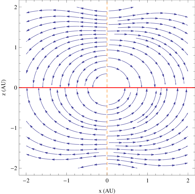
Figure 5: Projection in the plane $(x,z)$ of the streamlines of the drift velocity of charged particles moving in the heliosphere. The figure is valid for $qA>0$. The direction Changing the sign of the electric charge or the polarity of the solar phase the direction of the drift is reversed.

The streamlines of the drift velocity are shown in fig.5. Comparing these figure with the streamlines of the electric field shown in fig.4 one can notice that the directions of the drift velocity and of the electric force appear to be always antiparallel. In fact the scalar product of the drift velocity and the electrical force can be calculated explicitely with a result:

$$\left\langle\frac{dE}{dt}\right\rangle=q\,\vec{\boldsymbol{E}}\cdot\vec{v}_{\rm drift}=-\frac{|q|}{2}E\,w\;\frac{\rho^{2}(2R^{2}+\rho^{2})}{(R^{2}+\rho^{2})^{2}\,r}\;\left(\beta_{\perp}^{2}+2\,\beta_{\parallel}^{2}\right)$$ (24)

that is manifestly negative. This result is valid for any sign of the electric charge and of the solar polarity, because reversing the sign of $q$ or $A$ inverts the directions of both the electrical force and of the drift velocity, leaving the scalar product of the two vectors invariant. The scalar product $q\,\vec{\boldsymbol{E}}\cdot\vec{v}_{\rm drift}$, as indicated in equation (24), is equal to the energy variation of a charged particle that moves in the heliosphere on a trajectory controled by the electromagnetic field (after averaging over the fast gyration around the magnetic field lines). Equation (24) therefore states that the average energy variation is always negative, it is an energy loss.

It is instructive to compare equation (24) with the expression of the adiabatic energy loss used in the Parker equation for a relativistic particle diffusing in a spherically expanding wind:

$$-\left\langle\frac{dE}{dt}\right\rangle=|q|\,E\;\vec{\nabla}\cdot\vec{w}=\frac{2|q|\,E\,w}{r}~{}.$$ (25)

The expressions (24) and (25) are very similar, with identical dependences ($\propto|q|\,E\,w$) on the wind velocity and on the charge and energy of the particle, and similar dependence on the space coordinates (approximately $\propto r^{-1}$ in both cases). This similarity emerges because the expression of the adiabatic energy loss can be derived with magnetohydrodynamics consideration for the random magnetic field that are very similar to those developed here for the large scale regular field. The important difference between expression (24) and (25) is that the first case the energy loss can be associated to an electric potential, while in the other this is not possible. This point will be illustrated more extensively in section 5.

4 Space trajectories in the heliosphere

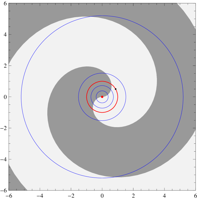
Figure 3: Section $xy$ of the inner part of the heliosphere. The Sun is at the center of the image, the circles indicate the orbits of the five inner planets (Mercury, Venus, Earth, Mars and Jupiter). The spiral that separates the darker and lighter regions marks the intersection of the heliospheric current sheet with the Earth’s orbital plane. In the darker (lighter) region the current sheet is below (above) the plane. In a positive polarity solar phase the magnetic field lines are directed toward (away from) the Sun below (above) the current sheet. For a negative polarity phase the field directions are inverted.

For a qualitative understanding of the problem we are discussing, it is very instructive to inspect some examples of trajectories of charged particles in the heliosphere, obtained with a numerical integration of the equation of motions (2). In the following calculations we will use a coordinate system where the Sun is at the origin and the $z$ axis is parallel to the Sun rotation axis; the orientation of the $x$ and $y$ axis with respect to the pattern of the HCS is chosen as shown in fig.3. One example of trajectory is shown in fig.6 for an electron that is “observed” at the Earth with energy $E=10$ GeV and direction with polar angles $\{\cos\theta=2/3,\varphi=3\pi/4\}$. At the “detection” time the phase of the Earth with respect to the pattern of the heliospheric current sheet was $\varphi_{\oplus}=0$, when the Earth (see fig.3) is above the heliospheric current sheet. The trajectory is calculated from this initial condition integrating the equations of motion both forward and backward in time. In the calculation the solar polarity is positive ($A>0$) and the parameters that describe the Sun magnetic field are $B_{0}=10^{-4}$ Gauss, $w=400$ km/s and $\sin\alpha=0.05$. Reversing simultaneously the polarity $A$ of the heliospheric magnetic field and the electric charge $q$ of the particle the trajectory remains identical and therefore the example of fig.6 refers more in general to the condition $qA>0$.

The particle of this example reaches the Earth, traveling on a down–going spiral that wraps around a surface of approximately paraboloidal shape, and then leaves the heliosphere traveling close to the equatorial plane, or more accurately close to the heliospheric current sheet.

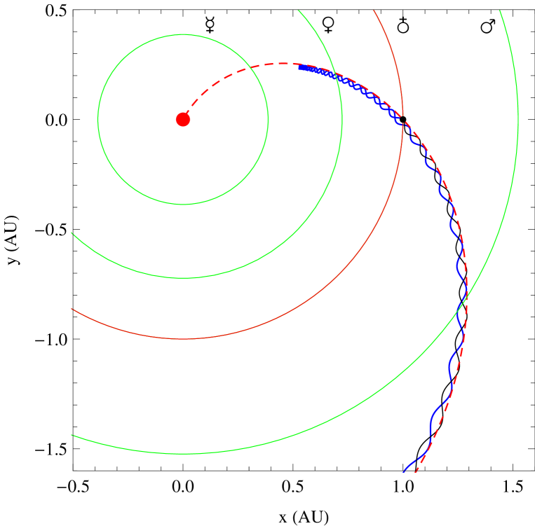
Figure 7: Projection in the $\{x,y\}$ plane of the space trajectory shown in fig.6. The thick (thin) line corresponds the portion of the trajectory before (after) the observation at the Earth. The dashed red line shows the magnetic field line that passes through the observation point.

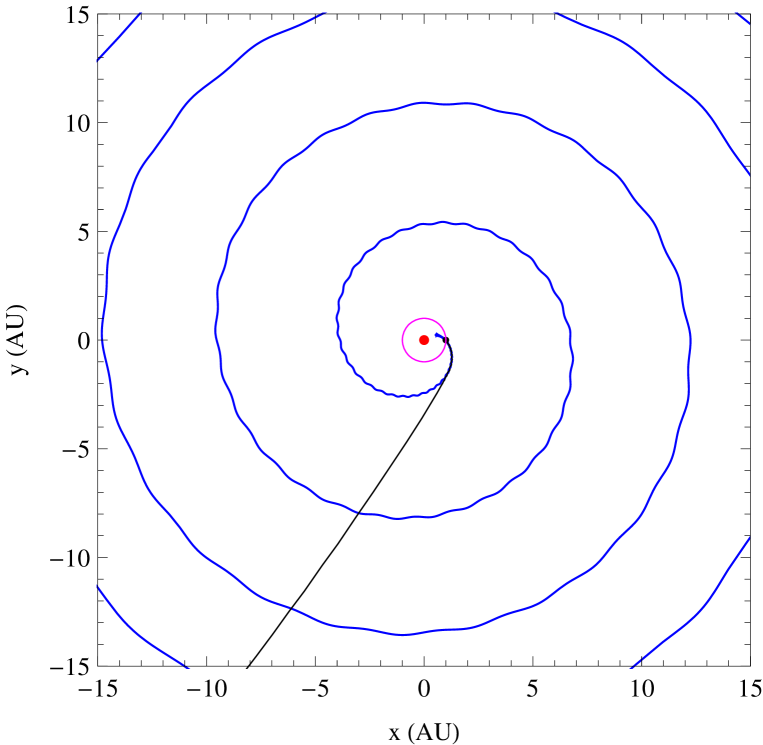
Figure 8: Same as fig.7 but with an enlarged scale.

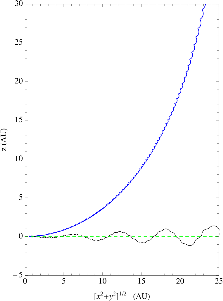
Figure 9: Projection in the $\{\sqrt{x^{2}+y^{2}},z\}$ space of the trajectory shown in fig.6 (a particle with observed energy 10 GeV). The thick (thin) line corresponds the portion of the trajectory before (after) the observation at the Earth.

For a better visualization, fig.7 and fig.8 show (with different scales) the projections of the trajectory in the equatorial {$x,y$} plane, while fig.9 shows the projection in the $\{\sqrt{x^{2}+y^{2}},z\}$ space. In fig.7 one can best see (in the $\{x,y\}$ projection) the trajectory in the inner part of the heliosphere. It is clear that, in first approximation, the particle gyrates around a magnetic field line (one such line is shown as a dashed curve in the figure). The trajectory also undergoes a “bounce”, (or a “reflection”) at the point of closest approach to the Sun, an example of the well known magnetic mirror effect, present when the magnetic field lines converge. Fig.8 and fig.9 allow to visualize the “in” part of the particle trajectory as a spiral wrapped around a paraboloid, and the “out” part as propagation close to the wavy heliospheric current sheet.

The main qualitative features of the trajectory we have just presented: the spiral, the bounce, and the outgoing travel close to the HCS, are in fact general features that are present in all trajectories when the product of the particle electric charge and of the solar polarity is positive ($qA>0$). The spiral is downgoing (as in our example) when the Earth is located above the HCS, but it is upgoing when the Earth is below the HCS. In the opposite case ($qA<0$) the trajectories have the same three features, but in reversed order. The particles enter the heliosphere traveling close to HCS, undergo a bounce at a point of closest approach to the Sun, and then exit the heliosphere traveling on a (upgoing or downgoing) spiral.

The qualitative features of the trajectories, are determined by the structure of magnetic field, (note that in the equations of motion the effects of the electric field are suppressed by a factor $w/c$, and can be considered as a as small perturbation), and are easy to understand qualitatively, using the results on the properties of the magnetic field lines and of the drfit velocity derived in the previous sections. The key points are the facts that the magnetic field lines are spirals around vertical cones, and that the drift velocity points toward (away from) the current sheet for $qA>0$ ($qA<0$).

For $qA>0$, when the drift “pushes” the particle toward the HCS, the charged particle can enter the heliosphere only traveling along a trajectory that starts at large $|z|$, and spirals around the $z$ axis following the behavior of the field lines. Since all magnetic field lines converge at the origin, and the convergence acts as a magnetic mirror, the particle trajectory will stop approaching the Sun, and will be reflected outward, undergoing a “bounce”. The qualitative behavior of the trajectory changes dramatically when the particle reaches the HCS. The magnetic drift effects (for the case $qA>0$ we are discussing now) always push the particle toward the HCS, so that it remains “trapped” close to the sheet (crossing it multiple times) while it travels out of the heliosphere.

A similar discussion can be applied to the case $qA<0$ to show that the trajectory is formed by the sequence of an “in” section, where the particle reaches the Earth traveling near the HCS, a bounce, and an “out” section that is an (upgoing or dowgoing) spiral around the $z$ axis.

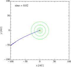
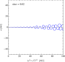
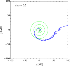
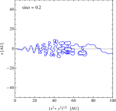
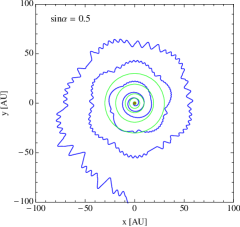
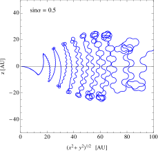
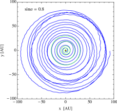
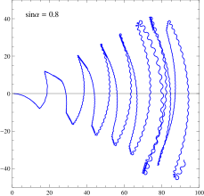
Figure 10: Projections of the past trajectory of an electron observed at the Earth with energy 10 GeV. The calculations are for $qA<0$. The trajectory is calculated for four different values of the tilt angle: $\sin\alpha=0.02$, 0.2, 0.5 and 0.8.

The properties of the “out” (“in”) part of the trajectories of charged particles for the case $qA>0$ ($qA<0$), depend strongly on the shape of the HCS, and in particular on the tilt angle $\alpha$, because the particle remains close the sheet, and follows its shape. This is illustrated in fig.10 that shows (for the case $qA<0$) the past (or “in”) trajectories of $e^{\pm}$ observed at the Earth with $E=10$ GeV. The trajectories are shown in two projections ($\{x,y\}$) and ($\{\sqrt{x^{2}+y^{2}},z\}$), for four different values of the tilt angle ($\sin\alpha=0.02$, 0.2, 0.5 and 0.8). For small tilt angle (as already shown in the example of fig. 6–9) the past trajectory is approximately radial and confined to the heliospheric equatorial plane. For large tilt angle the trajectory undergoes oscillations around the the equatorial plane with an amplitude that increases with $\sin\alpha$ and $\sqrt{x^{2}+y^{2}}$ reflecting the shape of the heliospheric current sheet; at the same time the trajectory rotates around the $z$ axis following the shape of the field lines.

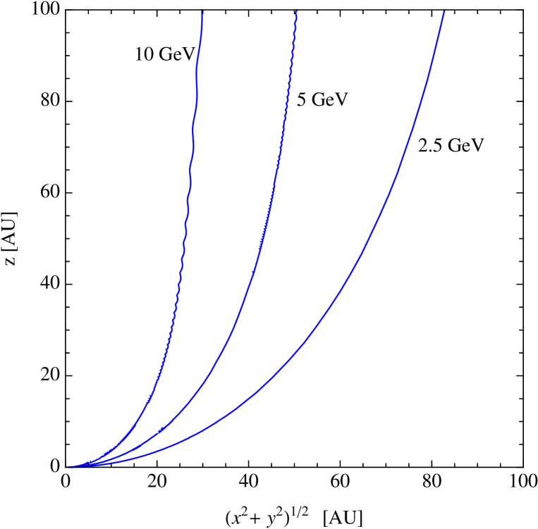
Figure 11: Projection of the “in” part of the space trajectories of $e^{\pm}$ observed at the Earth with energy $E=2.5$, 5 and 10 GeV. The calculation is for $qA>0$.

The spirals that form the “in” trajectories when $qA>0$ and the “out ”trajectories when $qA<0$ have a shape that is independent from the tilt angle of the HCS, because they remain on one side of the HCS. The projection of the spiral in the $\{\sqrt{x^{2}+y^{2}},z\}$ plane has a quasi–parabolic shape that depends on the particle momentum as illustrated in fig.11, that shows this projection for three particle momenta. The energy dependence of the shape can be understood as the consequence of a drift velocity that is proportional to the particle energy.

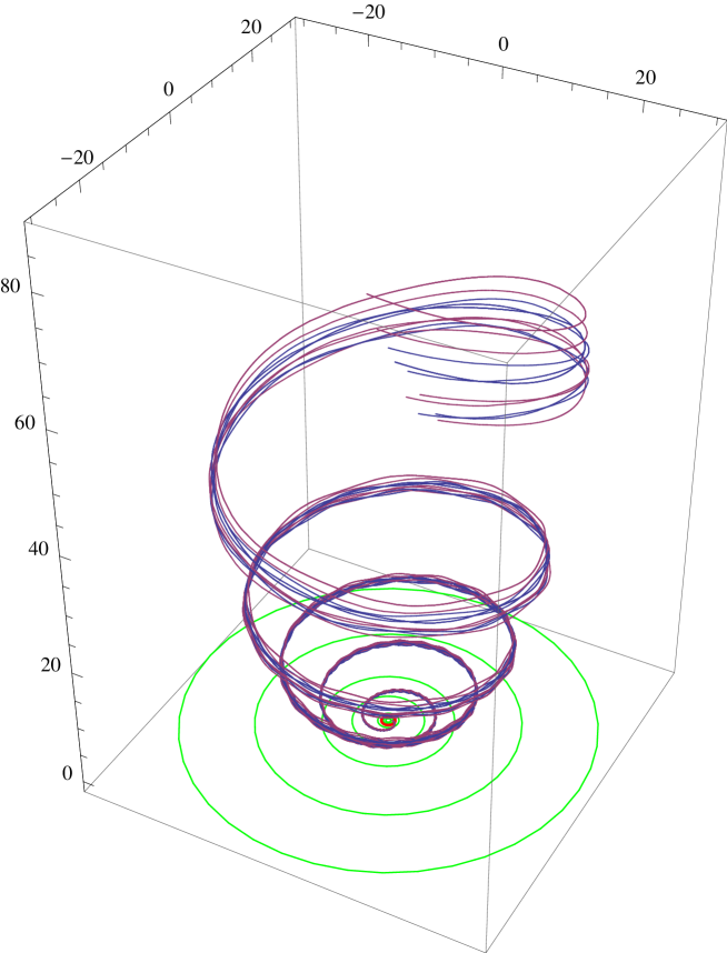
Figure 12: Past trajectories of $e^{\pm}$ that arrive at the Earth with energy 12 GeV and different directions. The calculation is valid for $qA>0$.

Note that the asymptotic direction (for $t\to-\infty$) of the particle has polar angle $\theta$ that is approximately 0 or $\pi$, for upgoing or down going spirals. This property is also illustrated in fig.12 and 13 that show the past trajectories of particles observed at the Earth with 12 GeV, and different directions that span the entire solid angle at the detector point. One can see that for $t\to-\infty$ the directions of all particles converge to the same one (that is approximately $\theta=0$).

5 Energy Loss

The equations of motion for the propagation of a charged particle in the heliosphere imply an energy variation given by:

$$\frac{dE}{dt}=q\;\frac{d\vec{x}}{dt}\cdot\vec{\boldsymbol{E}}$$ (26)

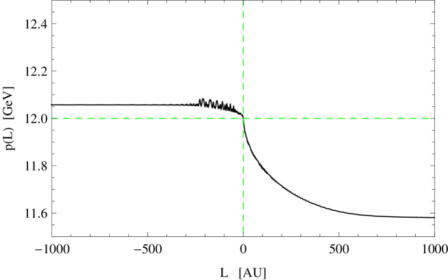
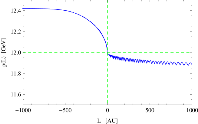
Figure 14: Energy evolution of an $e^{\pm}$ particle observed at the Earth with energy 12 GeV plotted as a function of the length $L=c\beta\,t$ (in astronomical units) along the trajectory. The top (bottom) panel is for $qA>0$ ($qA<0$). The space trajectory for the case $qA>0$ is shown in figures 6–10.

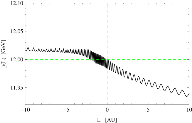
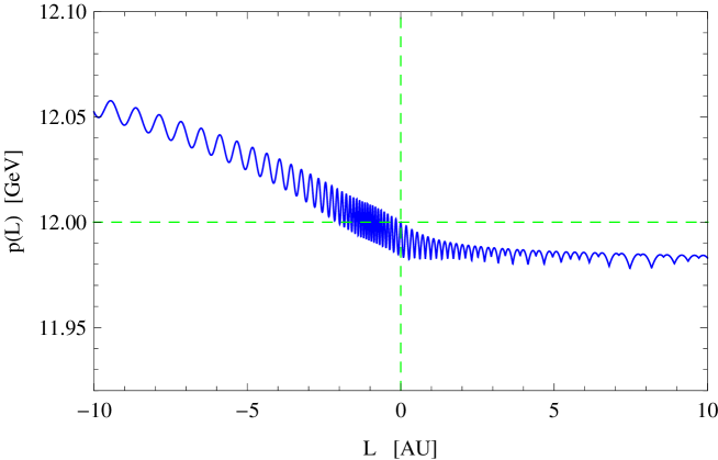
Figure 15: Energy evolution of an $e^{\pm}$ particle observed at the Earth with energy 12 GeV (the space trajectory is shown in fig.6) plotted as a function of the length $L=c\beta\,t$ (in astronomical units) along the trajectory. The top (bottom) panel is for $qA>0$ ($qA<0$).

Two examples of this energy evolution, for an $e^{\pm}$ observed at the Earth with $E=12$ GeV are shown in fig.14 that plots the energy as a function of the length along the trajectory. The portion of the trajectories closest to the Earth is also shown on an enlarged in fig.15. In the example the parameters of the heliospheric field are: $B_{0}=10^{-4}$ Gauss, $w=400$ km/s and $\sin\alpha=0.05$.

Inspecting the figures, one can see that after averaging for the small, fast oscillations (produced by the gyration motion around the magnetic field lines, that rapidly change the orientation of the particle velocity with respect to the electric field), the particles continuosly lose energy, both entering and exiting the heliosphere. This behavior was predicted in section 3 and with equation (24). The initial energy of the particle $E_{i}=E_{\rm obs}+\Delta E$ can be obtained as the limit of $E(t)$ for $t\to-\infty$, and depends on the sign of the particle. For $qA>0$ one has $\Delta E_{+}\simeq 0.42$ GeV for $qA<0$, $\Delta E_{-}\simeq 0.12$ GeV.

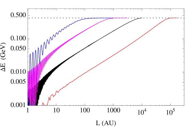
Figure 16: Time evolution (in the past) of the energy of $e^{\pm}$ observed at the Earth with energy of 1, 3, 10 and 30 GeV. for the case $qA>0$. The direction of the particle at the Earth and the position of the Earth is equal for all particles.

Figure 16 shows (for the same configuration of the heliospheric fields) the past time evolution of four particles (in the case $qA>0$) that reach the Earth with energy 1, 3, 10 and 30 GeV. The remarkable thing, that is immediately apparent inspecting the figure, is that the energy loss suffered by all particles (in this case for $qA>0$) that reach the Earth is equal, (and with value 0.42 GeV). From fig.16 one can also see that the time needed by a charghed particle to reach the Earth from the boundary of the heliosphere has the energy dependence $E^{-1}$, reflecting a drift velocity proportional to $E$. On the other hand, as shown in equation (24), the energy loss $-dE/dt$ is proportional to $E$. Combining the two effects one arrives to a total energy loss that is independent from energy.

The result that the energy loss of particles that reach the Earth for $qA>0$ is a constant (for fixed values of $B_{0}$ and $w$) can be easily seen as an elementary consequence of the existence of an electric field potential (as given in equation (16)), and of the fact that the trajectories are spirals around the heliospheric $z$ axis.

The energy variation of a charged particle that follows a trajectory $T$ can be calculated performing the line integral:

$$E_{f}=E_{i}+q\,\int_{T}d\vec{\ell}\cdot\vec{\boldsymbol{E}}(\ell)$$ (27)

Because of the existence of the electric potential, if the trajectory never crosses the heliospheric current sheet (where the electric potential is discontinuos), the energy loss $\Delta E=E_{i}-E_{f}$ is given by:

$$\Delta E=q\left[V(\vec{x}_{f})-V(\vec{x}_{i})\right]~{}.$$ (28)

and is proportional to the difference between the electric potential calculated at the initial and final point on the trajectory.

More in general, for a trajectory that crosses $n$ times the heliospheric current sheet, one has:

$$\Delta E=q\left[V(\vec{x}_{f})-V(\vec{x}_{i})\right]+q\;\left[\sum_{k=1}^{n}\Delta V_{\rm disc}(\vec{x}_{k})\right]$$ (29)

where the summation is over all points $\{\vec{x}_{k}\}$ of intersection of the trajectory with the HCS, and $\Delta V_{\rm disc}(\vec{x}_{k})$ is the potential jump at the discontinuity.

An alternative way to write the result (29) is:

$$\Delta E=-q\;\left[\sum_{j=1}^{n+1}\Delta V_{j}\right]\;,$$ (30)

that is as the sum of the contributions as in equation (28) of the ($n+1$) trajectory segments that divide the trajectory, having the points of discontinuity for the potential only at the boundaries.

The result (28) is sufficient to compute the energy variation in the case $qA>0$. In this case the charged particles reach the Earth traveling on a (downgoing or upgoing) spiral, starting from a very large value of $|z|$, and (with very few exceptions) arrive at the Earth without ever crossing the HCS. The energy loss can then be estimated as:

$$\left.\Delta E\right|_{qA>0} = q\left[V(z=0)-V(|z|\to\infty)\right]$$ (31)

$$= +q\,A\,|V_{\infty}|=+|q|\;|V_{\infty}|~{}.$$

In the the first step in the second line we have used the fact that the potential at $z=0$ vanishes, and equation (17) for the value of the potential at $|z|$ large. In the final step we have used the condition $qA>0$. Substituting the expression of the potential at large $z$ $|V_{\infty}|$ given in equation (17) one finds the energy loss:

$$\left.\Delta E\right|_{qA>0}=Z\,|q_{e}|\;B_{0}\,\frac{\Omega\,r_{0}^{2}}{c}\simeq 0.422\;Z\;\left(\frac{B_{0}}{10^{-4}~{}{\rm Gauss}}\right)~{}{\rm GeV}~{}.$$ (32)

It is less straightforward to estimate the energy loss for the case $qA<0$. In this case the magnetic drift pushes the particle away from the heliospheric current sheet, and therefore the particles can arrive at the Earth only traveling close the heliospheric equator. Since the points $\vec{x}_{f}$ (the Earth position) and $\vec{x}_{i}$ (where the particle enters the heliosphere) have both $z$ coordinate close to zero, one has $V(\vec{x}_{i})\simeq V(\vec{x}_{f})\simeq 0$, and the first term in the right hand side of equation (29) vanishes. On the other hand the particles traveling close to the HCS will cross it several times, and the second term in the equation (that sums the potential jumps at the discontinuities) contributes to the energy variation.

It is easy to see that also in this case one has an energy loss, because the drift is always against the direction of the electric force. The energy loss for the case $qA<0$ is however sensitive to the value of the HCS tilt angle, and in fact depends approximately linearly on $\sin\alpha$.

Having defined the electric potential with the convention that $V=0$ for points on the heliospheric equator, one has the potential on the two sides of the HCS are equal and opposite. Using equation (16) one has:

$$V_{\pm}=\mp A\,|V_{\infty}|\;\frac{z}{r}$$ (33)

The points on the sheet have $|z|/r$ in the interval $0\leq|z|/r\leq\sin\alpha$, so that the each crossing of the HCS gives a contribution to the energy loss in the interval:

$$0\leq\Delta E_{k}=q\;\Delta V_{\rm disc}(\vec{x}_{k})\leq 2|q|\,|V_{\infty}|\,\sin\alpha~{}.$$ (34)

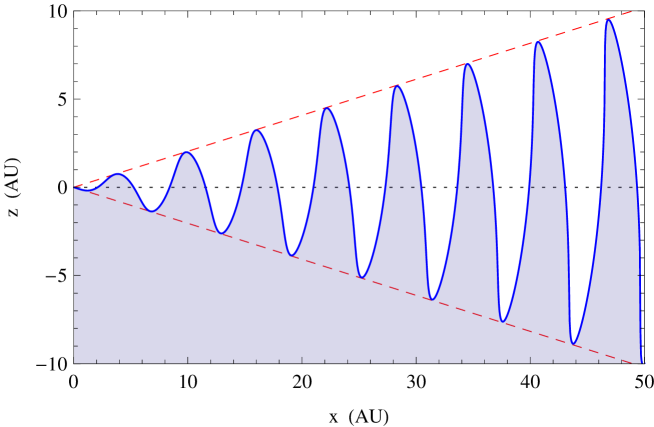
Figure 2: Section $xz$ of the heliospheric current sheet. For positive polarity ($A>0$) the field lines enter (exit) the plane of the figure in the white (shaded) area. The dashed lines correspond to the condition $\cos\theta=\pm\sin\alpha$ (with $\theta$ is the standard the polar angle and $\alpha$ the tilt angle of the heliospheric field). For a negative polarity phase the field directions are inverted.

The points on the HCS that satisfy the condition $V=\pm|V_{\infty}|\sin\alpha$ are those on the crests of the waves in the ondulating HCS (see fig.2). Equation (34) implies that for small tilt angle, when the HCS nearly coincides with the equatorial plane, all $\Delta E_{k}$ (and therefore $\Delta E$) are small.

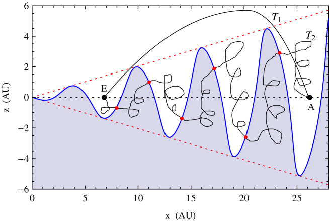
Figure 17: The figure shows an $\rho z$ section of the heliosphere. The wavy line is the heliospheric current sheet that separates regions of space where the field lines enter and exit the page. Note that the points on the current sheet that also satisfy the condition $z=\sin\alpha\,x$ (or $z=-\sin\alpha\,x$) have equal potential. Points $A$ and $E$ have the same potential. The line integral of the electric field along the trajectory $T_{1}$ is zero, while the line integral along $T_{2}$ that crosses several times the current sheet is non vanishing.

For a visualization of the energy loss in the case $qA<0$ one can inspect fig.17 that illustrates schematically the propagation of a charged particle (in the case $qA<0$) from a point A on the heliospheric equator to point E (the Earth). Both the starting and final points of the trajectory are at $z=0$ and have electric potential ($V=0$), therefore the line integral of the electric field along any trajectory (like $T_{1}$ in the figure) that does not cross the HCS vanishes. On the other hand the dynamically possible trajectories that connects the points A and E, looks schematically like $T_{2}$. The magnetic drift pushes the particle toward $+z$ ($-z$) when the particle is above (below) the HCS, however the trajectory meets and crosses several time the HCS because of the waviness of its shape. In each segment of the trajectory between HCS crossings, the particle loses energy because it moves against the electric force that always points in a direction opposite to the drift, that is toward $-z$ ($+z$) above (below) the HCS, so that the particle continuously loses energy.

The total energy loss of the particles that reach the Earth in the case $qA<0$ is not unique, because it depends on how many times and at what points a particle crosses the HCS. Numerical studies indicate however that the loss has a surprisigly small dispersion. As it is intuitive looking at equation (34) the average energy loss is proportional to the product $|V_{\infty}|\;\sin\alpha$, so that

$$\left.\left\langle\Delta E\right\rangle\right|_{qA<0}=f~{}|q|\;|V_{\infty}|\;\sin\alpha$$ (35)

Numerical experiments suggest a value $f\simeq 1.5$–2.5.

The results (31) and (35) can be summarized as:

$$\Delta E\simeq\begin{cases}|q|\,|V_{\infty}|&\mbox{for }qA>0~{},\\[5.69046pt] |q|\,|V_{\infty}|\;f\,\sin\alpha&\mbox{for }qA<0~{}.\end{cases}$$ (36)

The quantity $f$ is of order 2, and the potential of $V_{\infty}$, given in equation (17), depends on the absolute normalization of the heliospheric magnetic field. Numerically one has:

$$|q|\,|V_{\infty}|=Z\,|q_{e}|\;B_{0}\,\frac{\Omega\,r_{0}^{2}}{c}\simeq 0.422\;\left(\frac{B_{0}}{10^{-4}~{}{\rm Gauss}}\right)~{}{\rm GeV}~{}.$$ (37)

Both $B_{0}$ and the tilt angle $\alpha$ depend on the solar magnetic activity and vary with time.

The energy loss depends on the sign of the electric charge, and the role of particles with positive or negative charge is exchanged when the solar polarity is reversed. The energy loss is larger for the case $qA>0$ when the tilt angle is small ($\sin\alpha\lesssim 0.5$), and is larger for the case $qA<0$ when the tilt angle is large ($\sin\alpha\gtrsim 0.5$).

6 Energy Spectra

The fundamental problem in the study of solar modulations is to relate the energy spectra observed near the Earth at different times, to one unmodulated spectrum that gives the distribution at the boundary of the heliosphere. The unmodulated spectrum is assumed to be approximately stationary (on a time scale of order 10–100 years) and is commonly called the “Local Interstellar Spectrum” (or LIS).

In the model described here, and with the approximation that charged particles lose a well defined energy $\Delta E_{\pm}(t)$ (given by equation (36)) the problem has a simple closed form solution. Calling $\phi_{\rm obs}(E,t)$ the observable flux at the Earth, and $\phi_{0}(E)$ the LIS, one has:

$$\phi_{\rm obs}(E,t)=\phi_{0}[E+\Delta E(t)]~{}\left[\frac{E^{2}-m^{2}}{[E+\Delta E(t)]^{2}-m^{2}}\right]~{}.$$ (38)

This result is also the well known expression of the so called “Force Field Approximation” (FFA) for the solar modulations [10].

The remarkable point is that in the context of the discussion here the “Force Field” is real, and is due to the electric field that fills the heliosphere, and the FFA expression of equation (38) is an exact (for $qA>0$) or nearly exact (for $qA<0$) result.

Equation (38) can be derived as a simple consequence of the Liouville theorem, that states that if the Lagrangian of a physical system is time independent, the phase space density of an ensemble of particles remains constant along a particle trajectory. More formally, denoting as $\rho(\vec{x},\vec{p},t)=d^{6}N/(d^{3}x\,d^{3}p)$ the phase space density, one has that if $\{\vec{x}(t_{1}),\vec{p}(t_{1})\}$ and $\{\vec{x}(t_{2}),\vec{p}(t_{2})\}$ are two points on one solution of the equations of motion then:

$$\rho[\vec{x}(t_{1}),\vec{p}(t_{1}),t_{1}]=\rho[\vec{x}(t_{2}),\vec{p}(t_{2}),t_{2}]~{}.$$ (39)

The FFA expression (38) follows from (39) and the assumptions that the interstellar spectrum at the boundary of the heliosphere is stationary and isotropic. The flux (differential in energy) is related to the phase space density by the equation:

$$\phi(E,\hat{p},\vec{x},t)\equiv\frac{dN}{dE\,\,dA\,dt\,d\Omega}=v\;p^{2}\;\frac{dN}{d^{3}p\,d^{3}x}\;\frac{dp}{dE}=p^{2}~{}\rho(\vec{x},\vec{p},t)$$ (40)

(with $E=\sqrt{p^{2}+m^{2}}$). The particle velocity cancels in the last equality because the Jacobian factor is $dp/dE=1/v$. From the condition that the phase densities of the particles at the Earth and outside the heliosphere are equal, one obtains a relation between the LIS and the observed spectrum. Using equation (40) and the assumptions that the phase space density at the boundary of the heliosphere is isotropic one then obtains:

$$\phi_{\rm obs}(E)\,p_{i}^{2}=\phi_{0}(E_{i})\,p^{2}$$ (41)

where $E$ and $p$ are the energy and momentum at the Earth, and $E_{i}$ and $p_{i}$ the same quantities outside the heliosphere. Equation (38) follows from the condition $E_{i}=E+\Delta E$.

The FFA algorithm of (38) is symmetric, and it can be used to compute the observable flux at the Earth from the LIS spectrum, or viceversa, to reconstruct the unmodulated LIS spectrum from the observations. For this purpose (dropping the time dependence of $\Delta E$ in the notation) one can recast the equation in the form:

$$\phi_{0}(E)=\phi_{\rm obs}[E-\Delta E]~{}\left[\frac{E^{2}-m^{2}}{[E-\Delta E]^{2}-m^{2}}\right]~{}.$$ (42)

In this case there is obviously a limitation, since equation (42), even in the case of a perfect meaurement, allows to determine the interstellar spectrum only above a minimum kinetic energy $\Delta E$, because for lower energy the argument of $\phi_{\rm obs}$ in (42) becomes unphysical, and the equation meaningless. This simply reflects the fact that particles with a kinetic energy lower than $\Delta E$ in interstellar space cannot reach the Earth.

It is interesting to note that equation (38) predicts that in the limit of small kinetic energy the observable flux at the Earth $\phi_{\rm obs}(E)$ is linear in $E_{\rm kin}$. In fact, in the limit $E_{\rm kin}\to 0$ (and for $E_{\rm kin}\ll m$) the observable flux has the behavior:

$$\phi_{\rm obs}(m+E_{\rm kin})\simeq\phi_{0}(m+\Delta E)\;\frac{2m\,E_{\rm kin}}{\Delta E^{2}+2m\,\Delta E}+O(E_{\rm kin}^{2})\simeq{\rm const}\times E_{\rm kin}~{}.$$ (43)

As it will shown in the following, the linear dependence of the fluxes is the observed behavior of the fluxes, and insures that the estimate of the interstellar flux $\phi_{0}(m+\Delta E)$ from equation (42) is finite.

More in general, it is possible to use expression (38) to relate spectra measured at different times. If for example the spectrum $\phi_{1}(E)$, measured at time $t_{1}$, is related to the LIS spectrum by the FFA expression with parameter $\Delta E_{1}$, and similarly the spectrum $\phi_{2}(E)$, measured at time $t_{2}$, is related to the LIS spectrum using the same relation with the parameter $\Delta E_{2}$, then the spectra $\phi_{2}(E)$ can be obtained from the flux $\phi_{1}(E)$ with the one parameter transformation:

$$\phi_{2}(E)=\phi_{1}[E+\Delta E_{21}]~{}\left[\frac{E^{2}-m^{2}}{[E+\Delta E_{21}]^{2}-m^{2}}\right]~{}.$$ (44)

where

$$\Delta E_{21}=\Delta E_{2}-\Delta E_{1}~{},$$ (45)

or symmetrically $\phi_{1}(E)$ can be obtained from $\phi_{2}(E)$ by the same transformation with parameter $\Delta E_{12}=-\Delta E_{21}$. Equation (44) can be used to test experimentally the validity of the FFA, measuring two spectra for different conditions in the heliosphere, and studying if the spectra satisfy equation (44) for some value of the parameter $\Delta E_{21}$.

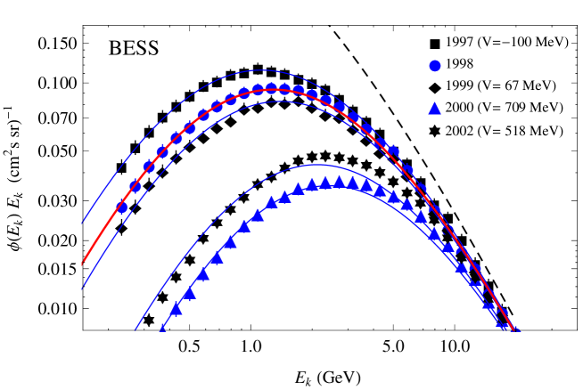
Figure 18: Proton spectra measured by the BESS collaboration at different times. [11, 12]. The thick red line is the fit to the 1998 BESS proton given in [12]. The other lines are one parameter fits to data, distorting the curve that describes the 1998 data the algorithm of the Force Field approximation. The best fit parameter of the curves is given in the figure.

An illustration of the FFA algorithm applied to measurements of the cosmic ray proton spectrum is given in fig.18 and 19 that show measurements of the proton flux measured at different times by the BESS [11, 12] and PAMELA [13] detectors. The BESS measurements were performed during (approximately one day long) balloon flights in 1997, 1998, 1999, 2000 and 2002. During all this time the polarity of the heliospheric magnetic field was positive ($A>0$). The measurements of PAMELA are averages of data collected in 2006, 2007, 2008 and 2009, when the polarity of the heliospheric field was negative ($A<0$).

Fig.18 shows the five measurements of the BESS spectrometer [12]. In the figure the thick (red) line was chosen to give a good description of the data collected by BESS in 1998, the other lines are calculated using the FFA algorithm of equation (44) using the 1998 flux as starting point and fitting the parameter $\Delta E$ for the other BESS measurements of the proton flux performed in 1997, 1999, 2000 and 2002. The best fit values of $\Delta E$ (relative to the 1998 measurement) for the four spectra are $-100$, 67, 709 and 518 MeV. The parameter $\Delta E$ is positive (negative) when the fitted spectrum is lower (higher) than the reference flux.

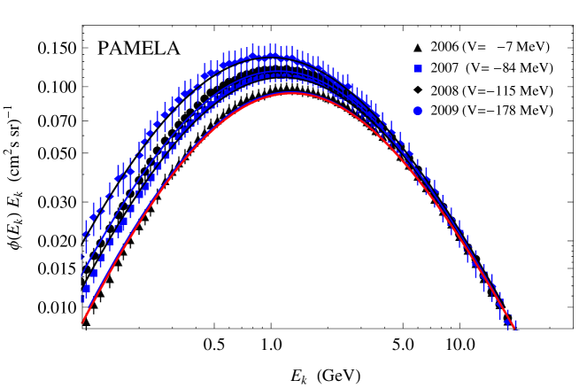
Figure 19: Proton spectra measured by the PAMELA collaboration [13]. The thick red line is the fit to the 1998 BESS proton data shown in fig.18. The other lines are one parameter fit to the PAMELA data, where the fitting curve is the fit to the BESS-1998 data, distorted with the algorithm of the Force Field approximation. The parameter of the fit is shown in the figure.

Figure 19 shows the measurements of the proton flux obtained by PAMELA [13] in 2006, 2007, 2008 and 2009. The lines in the figure are one parameter fits to the four spectra with the FFA algorithm of equation (44), calculated using as starting flux the parametrization of the measurement performed by BESS in 1998. The best fit values for $\Delta E$ are $-7$, $-84$, $-115$ and $-178$ MeV (in all years the flux measured by PAMELA is higher than the one measured by BESS in 1998). The FFA fits give a very good description of the proton spectra.

In summary, the measurements of the proton flux performed by BESS and PAMELA during nine years (that include an inversion of the solar magnetic phase) exhibit time variations that are reasonably well described by the Force Field Approximation algorithm.

In the discussion above, we have studied the validity of the FFA algorithm comparing measurements performed at different times, without attempting to reconstruct the unmodulated interstellar flux. Previous studies have used use the approach to relate the observed flux to the interstellar spectrum. For example, in [12] the BESS collaboration have shown the time dependence of their proton flux measurements also using the FFA algorithm, but starting from a model of the unmodulated LIS spectrum. This LIS spectrum (shown in fig.18 as a dashed line), is then used to estimate an energy loss $\Delta E$ (relative to the unmodulated flux) for each proton flux measurement. The two procedures (the one performed by the BESS collaboration, and the one discussed in this work) are perfectly consistent, because one has:

$$\Delta E_{j,1998}=\Delta E_{j,{\rm LIS}}-\Delta E_{1998,{\rm LIS}}~{},$$ (46)

where $j$ is an index that runs through the five measurements, $\Delta E_{j,1998}$ is the energy loss with respect to the 1998 measurement estimated in this work, and $\Delta E_{j,{\rm LIS}}$ the energy loss with respect to the LIS spectrum estimated by the BESS collaboration in [12]. In the BESS study the total energy loss of protons at the time of the 1998 measurement was estimated as 591 MeV.

The point we want to make here is that it is possible to verify the validity (or non–validity) of the FFA without making any assumption on the shape and properties of the interstellar flux, simply comparing measurements taken at different times, and testing if they are consistent with the one parameter transformation of equation (44). If this test is succesful, then one can conclude that all measurements are the results of the time dependent modulations of a unique interstellar flux described by the FFA algorithm.

Having established the validity (or approximate validity) of the FFA, the reconstruction of the unmodulated flux requires additional theoretical assumptions, because the FFA algorithm has in fact infinite solutions, parametrized by $\Delta E_{\rm LIS}$, that are mathematically all equally valid. To select the physically correct solution there are in principle two different methods. In the first, one starts from a theoretical prediction for the shape of the interstellar energy spectrum, and then use equation (42) to determine $\Delta E_{\rm LIS}$, as ther parameter that reproduces the observed spectrum, starting from the interstellarone. This method allows to obtain an estimate of the total size of the modulation effects from the cosmic ray flux measurement.

The alternative approach is to have a complete model for propagation in the heliosphere that allows to compute from first principles the value of $\Delta E_{\rm LIS}$ at different epochs. Inserting this value into equation (42) one can then calculate the of the interstellar energy spectrum from the observations of the spectral shape at the Earth.

The main point want to make in this section is that the FFA algorithm is quite successful in describing the time variations of the cosmic rays fluxes. This implies that the cosmic rays that arrive at the Earth lose a (time dependent) $\Delta E$ that is approximately equal for all energies and has a small dispersion.

In general one can expect that the relation between the observed and the interstellar flux is more complicated that the FFA algorithm of equation (38). For example, the energy variation $\Delta E$ could be a function of $E$ (or equivalently of $E_{i}$). Also in general the energy loss of particles that traverse the heliosphere will not be unique, but can have a distribution with a certain (possibly energy dependent) width and shape. The point os that the approximate validity of the FFA is non trvila result, that gives important constraints on the construction of a model of the solar modulations.

7 Summary and outlook

In this work we have studied the propagation of charged particles in the heliosphere assuming only the presence of the regular magnetic field, completely neglecting the random magnetic field generated by turbulent motions in the heliospheric plasma. The presence of a magnetic field in the solar wind, a moving plasma with good electrical conductivity, generates an electric field that plays an important role in the propagation of charged particles in the heliosphere, and results in significant solar modulations.

The combined effect of the large scale heliospheric magnetic and electric fields is that charged particles that reach the Earth from the boundary of the heliosphere always lose energy. The energy loss $\Delta E$, to a good approximation, is independent from the energy and direction of the particle, and is determined only by the structure of the heliospheric fields. The energy loss is proportional to the absolute value of the electric charge of the particle, but depends on the sign of the charge.

It might appear surprising that the same field configuration can generate energy losses for particles of opposite electric charge, but this is possible because particles of opposite charge reach the Earth traveling on different trajectories. In all cases the electric field results in a force that, after averaging over fast gyrations around the magnetic field lines, is anti–parallel to the particle velocity, and causes an energy loss.

The shape and properties of the trajectories are determined by the structure of the heliospheric magnetic field, with the electric field that acts effectively only as a small perturbation. When the product $qA$ of the particle electric charge and the solar magnetic polarity is positive particles arrive at the Earth traveling along spirals around the heliosphere polar axis, in the opposite case the particles arrive traveling close to the heliospheric current sheet (HCS) and the the heliospheric equator.

The energy loss is always linear with the value pof the magnetic field, but in the case $qA<0$ it also depends on the tilt angle of the HCS, and is also linear with $\sin\alpha$. The energy loss is larger for $qA>0$ when the tilt angle of the HCS is small ($\sin\alpha\lesssim 0.5$), and it is larger for $qA<0$ when the tilt angle is large ($\sin\alpha\gtrsim 0.5$). A quantitative estimate of the energy loss is given in equations (36) and (37), and is of order of a few hundred MeV.

All the results discussed in this work have been obtained for a very simple model of the heliosphere (a magnetic field that is a Parker spiral, and a solar wind that is purely radial, and of constant velocity), but one can expect that they will remain valid for a more general description of the heliospheric magnetic field and of the solar wind.

In conclusion, in this work we have demonstrated that the deterministic propagation of charged particles in the heliosphere results in an energy loss that is sufficient to generate important solar modulations.

Modern calculations of solar modulations effects do include a description of the regular heliospheric magnetic field, but only as a convection term associated to the magnetic drift velocity. The drift velocity inverts its direction for the transformation $q\to-q$, and introduce a dependence on the sign of the electric charge. This treatment does not take into account properly of the important fact, outlined in this work, that the heliosphere contains a regular electric field, with a large scale structure. In the standard treatment of the solar modulations particles lose energy adiabatically, that is they suffer an energy loss proportional to energy and to the divergence of the wind velocity ($-dE/dt\propto E\,\nabla\cdot\vec{w}$). This implies that the total energy loss of a particle observed at the Earth is proportional to the time that a particle takes to penetrate the heliosphere, independently from the characteristics of the trajectories.

The phenomenological success of the Force Field Approximation (as discussed in section 6) suggests that charged particles penetrate the heliosphere losing an amount of energy $\Delta E$ that is approximately independent from $E$ and has a small dispersion. This is a suprising result when seen in the framework of the Parker equation, because it implies that the time needed by a particle to reach the Earth has the energy dependence $t\propto E^{-1}$, and therefore that the diffusion coefficient (that describes the effects of the turbulent magnetic field) has the energy dependence $D(E)\propto E$. This energy dependence of the diffusion coefficient is not seen in other astrophysical environments, for example when studying the escape of cosmic rays from the Milky Way, where one estimate a power law dependence $D(E)\propto E^{\delta}$ with $\delta=0.3$–0.6. Also the apparent narrowness of the $\Delta E$ distribution appears to be problematic.

These difficulties could perhaps be solved assuming that a large fraction of the energy loss for cosmic rays that travel in the heliosphere is caused by a large scale electric field that permeates the solar wind. The existence of this electric field emerges as a simple and well known magnetohydrodynamical effect when a conducting and moving fluid (such as the solar wind) contains a magnetic field. The investigation of this hypothesis clearly requires detailed numerical studies of the propagation of particles in the heliosphere that take into account the presence of both the regular and random components of the electromagnetic fields.

The existence of the regular electromagnetic fields in the heliosphere has very important consequences for studies on anisotropy of cosmic rays at the Earth, because it clearly has effects on the angular distribution of particles observed at the Earth. his problem will be discussed in a separate work [14].

In conclusion, the results outlined in this work point to the need of a profound revision of the treatment of solar modulations that properly include the regular electromagnetic fields present in the heliosphere.

Figure 6: Space Trajectory of an electron in the heliosphere. The particle is observed at the Earth with energy 10 GeV. The thick (thin) line shows the trajectory before (after) the observation. The green circles are the trajectories of the planets.

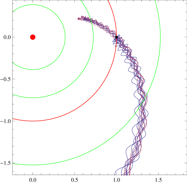
Figure 13: Projection in the equatorial plane of the “in” part of the trajectories of $e^{\pm}$ that arrive at the Earth with energy 12 GeV and different directions. The calculation is valid for $qA>0$.

References

- [1] M. Potgieter, Living Rev. Solar Phys. 10, 3 (2013) [arXiv:1306.4421 [physics.space-ph]].
- [2] E.N. Parker Planetary and Space Science 13, 9 (1965).
- [3] M. L. Goldstein, L. A. Fisk and R. Ramaty, Phys. Rev. Lett. 25, 832 (1970).
- [4] R. D. Strauss, M. S. Potgieter and S. E. S. Ferreira, Adv. Space Res. 49, 392 (2012).
- [5] J. R. Jokipii, E. H. Levy & W. B. Hubbard, Ap.J. 213, 861 (1977).
- [6] P. Bobik et al., Astrophys. J. 745, 132 (2012) [arXiv:1110.4315 [astro-ph.SR]].
- [7] L. Maccione, Phys. Rev. Lett. 110, no. 8, 081101 (2013) [arXiv:1211.6905 [astro-ph.HE]].
- [8] M. S. Potgieter, Adv. Space Res. 53, 1415 (2014).
- [9] J.D. Jackson, “Classical Electrodynamics//, 3rd ed. Wiley, 1998.
- [10] L. J. Gleeson and W. I. Axford, Astrophys. J. 154, 1011 (1968).
- [11] T. Sanuki et al. [BESS Collaboration] Astrophys. J. 545, 1135 (2000) [astro-ph/0002481].
- [12] Y. Shikaze et al. [BESS Collaboration] Astropart. Phys. 28, 154 (2007) [astro-ph/0611388].
- [13] O. Adriani et al. [PAMELA Collaboration] Astrophys. J. 765, 91 (2013) [arXiv:1301.4108 [astro-ph.HE]].
- [14] Paolo Lipari, in preparation.