Height distribution of equipotential lines in a region confined by a rough conducting boundary

Abstract

This work considers the behavior of the height distributions of the equipotential lines in a region confined by two interfaces: a cathode with an irregular interface and a distant flat anode. Both boundaries, which are maintained at distinct and constant potential values, are assumed to be conductors. The morphology of the cathode interface results from the deposit of $2\times 10^{4}$ monolayers that are produced using a single competitive growth model based on the rules of the Restricted Solid on Solid and Ballistic Deposition models, both of which belong to the Kadar-Parisi-Zhang (KPZ) universality class. At each time step, these rules are selected with probability $p$ and $q=1-p$. For several irregular profiles that depend on $p$, a family of equipotential lines is evaluated. The lines are characterized by the skewness and kurtosis of the height distribution. The results indicate that the skewness of the equipotential line increases when they approach the flat anode, and this increase has a non-trivial convergence to a delta distribution that characterizes the equipotential line in a uniform electric field. The morphology of the equipotential lines is discussed; the discussion emphasizes their features for different ranges of $p$ that correspond to positive, null and negative values of the coefficient of the non-linear term in the KPZ equation.

1 Introduction

Growth phenomena in non-equilibrium conditions [2, 3] are an important subject of condensed matter physics. Many properties of specific devices depend on rough surfaces that are produced under such non-equilibrium conditions. Technological applications such as conducting-field emitter devices that operate in Ultra High Vacuum (UHV) conditions, require the control of several properties such as the surface morphology. It is well known that large values of the current intensity on field emitter devices are connected to extremely small values of the effective emitting area [4]. One method to increase the effective area of emission is to use surfaces with an ending fractal boundary with self-affine scale invariance instead of considering structurally regular tips. In fact, the connection between the morphology of irregular surfaces including sharp conducting tips and the field emission properties has been a subject of intense research [5, 6]. In a recent work [7], Cabrera et al. measured experimentally the current-voltage (I-V) of a tunnel junction consisting of a sharp electron emitting metallic tip at a variable distance (“$\Delta$”) from a planar collector and emitting electrons using electric field assisted emission. Their results showed scale invariance of the tunnel junction with respect to changes in $\Delta$ (from few $mm$ to several $nm$), which means that the physical laws governing the flow of current are invariant with respect the changes of the length scale $\Delta$. However, this behavior fails when $\Delta$ was only a few nanometers as showed in reference [8]. The reported scale invariance for a single tip can be regarded as a preliminary study of the more general problem of field emission by an irregular conducting interface that will be considered in this work.

In the statistical mechanics framework, macroscopic laws that emerge in surface growth can be explained at different spatial and temporal scales considering a theoretical microscopic description that involves simple probabilistic laws. An interesting related point is the possibility of modeling these systems so that in the large-scale limit (i.e., where the scale invariance arises), they do not depend on the corresponding details but only on symmetries and the corresponding conservation laws.

Previous theoretical works related to the emitting properties of rough surfaces [9, 10, 11, 12, 13] have studied the behavior of the electric potential in a region bounded by a rough conducting profile/surface and a smooth conducting line/plane, which is held to a constant voltage bias. In particular, the references [10, 11] analyzed the roughness exponent of the equipotential lines (surfaces) in 2 (3)-dimensional systems. However, to our knowledge, no previous work discussed the properties of equipotential lines/surfaces under the perspective of its height distribution properties.

In this work, we investigate the height distribution properties of a family of equipotential lines in a region that is confined by a rough profile, which is regarded as an electron-emitting cathode, and a flat anode which is placed sufficiently away from it. The profile results from a numerical simulation of the deposition and growth surface models, whereas the cathode and the anode are subject to an electric potential difference. Our results are mainly based on the model that was introduced by Silva and Moreira [14, 15], which is compared to those obtained for the simpler Family model [16] in some limiting cases. We emphasize two consequences of our results for the following aspects: the height distribution presents a more detailed characterization of the equipotential lines than that provided by the roughness exponents and such investigation of equipotential lines offers a much more reliable method to characterize the surface. For particular applications, our work can contribute to elucidate the image distortions in probe microscopies such as Electrostatic Force Microscopy (EFM), where the knowledge of the electric field distribution along the tip probe is relevant to extract morphological information about the real irregular surface. This main conclusion from our work is particularly useful to study surfaces under the influence of non-linear mechanisms in the growth phase, where the surface width is not expressed as a power law with a single growth exponent for a large number of deposited monolayers.

This investigation is also motivated by the quoted experimental aspects related to the electronic properties of rough surfaces and the recent theoretical advances regarding the solution of the Kardar-Parisi-Zhang (KPZ) equation [17] in d = 1+1, where, in general, $d=n+1$ indicates that a system composed by a n-dimensional substrate (here, 1-dimensional) and an extra dimension to where an important effect produced by the substrate is propagated.

The remainder of the paper is organized as follows. In Sec. 2, we describe the main features of the used models and emphasize the conditions under which they reproduce the typical features of the KPZ and Edwards-Wilkinson (EW) [18] growth dynamics. In Sec. 3, we describe the methodology to calculate and characterize of the equipotential lines. In Sec. 4, we discuss our results for the morphological properties of equipotential lines and analyze the corresponding behavior of the skewness and kurtosis with the electric potential. In Sec. 5, we summarize the results and present our conclusions.

2 Models

It is convenient to discuss the properties of the computational surface growth models that are used in this work with those of the KPZ equation in $1+1$ dimensions

$$\partial_{t}h(x,t)=\mu_{0}+\nu\triangle h+\frac{\lambda}{2}(\nabla h)^{2}+\eta(x,t),$$ (1)

where $h(x,t)$ represents the height of the profile in the $y$ direction with respect to the line, $h(x,t=0)=0$, that describes the flat profile at $t=0$. Eq. 1 comprises several terms that consider the essential features of a stochastic surface growth. These features include irreversibility and locality, which enhance the surface roughness. In eq. 1 $\mu_{0}$ corresponds to a constant driving force, $\nu$ is the diffusion coefficient of the deposited atoms on the surface, and $\eta(x,t)$ is a white Gaussian noise that mimics the stochastic nature of the growth process. The non-linear term accounts for a considerable number of experimental results [19, 20] for the height distribution. Many of them cannot be described by a Gaussian function, which is the solution of the linear EW equation, which corresponds to setting $\lambda=0$ in eq. 1.

The investigated model depends on a parameter $p$, which describes the probability that the deposited particle follows the Restricted Solid on Solid (RSOS) local rule, whereas $q=1-p$ is the probability related to the Ballistic Deposition (BD) rule. Both RSOS and BD discrete models belong to the universality class that is defined by the KPZ equation but are characterized by negative and positive values of the parameter $\lambda$, respectively. Although the used model has not been proved to be equivalent to a KPZ equation, recent numerical investigations suggest that a change in the probability $p$ changes the value of $\lambda$ in a KPZ equation, which may be suitable to describe the competitive model [21, 22].

For almost all ranges of $p$, a growing profile first experiences a transient phase before attaining a stationary growth regime, where its width $W$ scales with the number of monolayers with the typical exponent $\beta_{KPZ}=1/3$ of the KPZ universality class. For finite profiles, this regime is interrupted when $W$ exponentially relaxes to a saturation regime and becomes constant. In this work, we analyze only rough interfaces in the growth regime, which corresponds to typical experimental conditions. In the first transient phase, depending on $p$, the growth exponent can reach values close to those typical of EW dynamics. Starting from $p=0$, the length of the transient phase increases until a specific value $p^{*}\approx 0.83$, where the EW typical value is always valid. For $p>p^{*}$, the model reaches KPZ scaling again after a decreasing transient time [23]. Because the condition $p=p^{*}$ is very special, we find it wise to compare the properties of the profiles and equipotential lines with those obtained when the cathode is represented by Family-model produced profile [16], which shows the EW properties notably clearly.

The interesting behavior of the competitive model makes it suitable to investigate how the equipotential lines change when $p$ is selected to reproduce either KPZ or EW dynamics, and for a fixed value of $p$, how the magnitude of the non-linear terms affects the EW-KPZ crossover as a function of time [23], which is particularly important for experimental interests. Indeed, the competition between physical mechanisms is present in many real processes in thin-film science. Then, the actual study clearly advances on the previously one where single models were considered, and the roughness exponent of equipotential lines were evaluated without a perspective for height distribution properties.

The distribution of height fluctuations of the KPZ equation, for a flat initial condition, can be expressed by Gaussian Orthogonal Ensemble (GOE) Tracy-Widom (TW) distributions [24]. Therefore our results can be better appreciated by comparing the skewness ($S$) and kurtosis ($K$) of the equipotential height distributions with the typical TW values for the corresponding quantities. Both $S$ and $K$ depend on the average distance from the equipotential lines to the cathode and anode. Such dependence has intrinsic features according to whether $p<p^{*}$ or $p>p^{*}$. A third distinct behavior is observed at $p=p^{*}$, when the profile falls into an EW universality class.

We emphasize again that our investigation opens the possibility of analyzing the effects on the behavior of equipotential lines of distinct surfaces with growth exponents near those that feature an EW class. This possibility is important because of the emergence of local growth exponents in the first transient growth phase, which is near the phase that characterizes the EW dynamics when $p\thickapprox p^{*}$. As shown in Sec. 4, our results indicate that the height distributions of equipotential lines for such transient patterns are clearly different from those obtained for an actual EW profile , no matter whether they are produced using the competitive model at $p=p^{*}$ or the Family model.

3 Methodology: Determination and Characterization of Equipotential Lines

The current investigation starts by constructing the rough profile $h(x)$, which acts as the cathode and results from one of the quoted deposition models. Here, $x$ and $y$ are integer numbers that represent distance measured in terms of some basic unit distance $u$, the precise size of which is not important in a theory of the kind under discussion. The growth process along the $y$ direction of the considered $1+1$ system (one-dimensional substrate + height, as mentioned in Sec.1) starts with a flat substrate $h(x,t=0)=0$, where $x$ is an integer number, and $x\in[1,L]$. The column height $h(x)$ is the $y$ coordinate of the topmost adatom at position $x$. We have used profiles with lateral size up to $L=10^{6}$ and up to $T=2\times 10^{4}$ deposited monolayers (ML). For such parameter values, finite-size effects no longer influence the interpretation of our results and can be neglected. During the growth process, the number of monolayers is also referred to as the integration time $t$; in this way, each time unit corresponds to the deposition of $L$ particles. For the convenience of using a unified notation for all profiles and equipotential lines, let us switch from $h(x)$ to $h(x,t)=h_{p,\phi}(x,t)$, where we emphasize the dependence of $h(x)$ on $t$. The subscript $p$ stands for the probability of choosing the RSOS rule in the competitive model. Finally, the subscript $\phi$ is used to identify the constant value of the equipotential line. In this work, $\phi=0$ and $\phi=A$ correspond to the cathode and anode surfaces, respectively.

The flat anode, which is defined by $h_{p,A}$, is placed at a distance $\langle d\rangle$ away from the cathode. $\langle d\rangle$ is measured by the number of vertical spacings between the average height of the profile $\overline{h}_{p,0}=\frac{1}{L}\sum\limits_{x=1}^{L}\left[h_{p,0}(x,T)\right]$ and the flat anode, i.e:

$$\langle d\rangle=h_{p,A}-\overline{h}_{p,0}.$$ (2)

As previously indicated, $\overline{h}_{p,0}$ is evaluated at $t=T$, except if explicitly indicated.

To compare the results for different rough profiles, we fixed the value of $\langle d\rangle$. As a consequence $h_{p,A}$, which is measured with respect to the substrate where the film is grown, changes with $p$. In this way, to select a proper and fixed value of $\langle d\rangle$, such that for any value of $p$ the anode is sufficiently away from the cathode, we first determined the value of $p$ for which the roughness $W$ (defined in eq. 4) attains its maximum, which is $p=0$ when $W\approx 37.3$. Next, we identified the vertical coordinate of the highest peak $h^{p=0}_{max}$ for this value of $p$ and set $h_{0,A}=h^{p=0}_{max}+\Delta$, which result, using eq. 2, in:

$$\langle d\rangle=h^{p=0}_{max}+\Delta-\overline{h}_{0,0},$$ (3)

where $\Delta$ corresponds to the distance defined on the second paragraph of Sec.1. At this point, let us comment on the reasons to choose the particular value of $\Delta$ used in this work. For $\Delta>>h^{p=0}_{max}$, the results are expected to be largely independent of the precise value of $\Delta$, but the computational work is largely increased. We have observed that, for all the rough profiles, the equipotential lines become flat and parallel to the $x$ axis very rapidly after the value of $y$ surpasses the highest peak. Therefore, we choose the value $\Delta=10$, which corresponds to $\langle d\rangle=198$. We use this average distance for all $p$, because it is already sufficient large to have very smooth equipotential lines (with roughness exponent, $\alpha$, near to unity [11]) that are observed at the flat anode. If we consider the basic unit distance $u=5$ nm, we obtain $\Delta=50$ nm for $p=0$, and $\langle d\rangle\simeq 1$ $\mu$m, which correspond to the typical scale used in the non-contact mode in atomic force microscopy (like EFM) where the electrostatic force is probed. Then, the results of this work can motivate experimental realizations in this regime.

Observed at this angle, the geometrical set up depends on two different scales (expressed by $L$ and $H$) along the horizontal and vertical directions. However, the rough profile has its own length scale in the vertical direction, which is the roughness

$$W_{p,0}(L,t)=\left[L^{-1}\sum\limits_{x=1}^{L}\left(h_{p,0}(x,t)-\overline{h}_{p,0}(t)\right)^{2}\right]^{1/2}$$ (4)

where $\overline{h}_{p,0}(t)=L^{-1}\sum\limits_{x=1}^{L}[h_{p,0}(x,t)]$.

When $t=T$, the profiles that are grown using the competitive model are in the asymptotic growth regime ($W\sim t^{\beta_{KPZ}}$) for $p\in[0,0.75)\bigcup(0.9,1]$. This regime corresponds to typical experimental conditions, in contrast to the exponential relaxation that is observed in steady-state (long-time) properties. For $p\in[0.75,p^{*})\bigcup(p^{*},0.90]$, the asymptotic growth KPZ regime has not yet been reached, and the system is in the EW-KPZ crossover [25, 26]. For $p=p^{*}\approx 0.83$, the system is in the critical point and the corresponding growth regime is such that $W\sim t^{\beta_{EW}}$, where $\beta_{EW}=1/4$ is the EW growth exponent.

The next step is to compute the equipotential lines, $h_{p,\phi}(x)$. Hence, we numerically solve Laplace’s equation

$$\nabla^{2}\phi=0,$$ (5)

for the electric potential $\phi$ in the region between the two conductors, which are held at constant potential values of $\phi^{C}$ and $\phi^{A}$ for the rough cathode and the flat anode that is parallel to the $x$ axis, respectively. The equation is solved using Liebmann’s method and the appropriate Dirichlet conditions. The geometrical characterization of the equipotential lines is insensitive to the choice of $\phi^{C}$ and $\phi^{A}\neq\phi^{C}=0$. However, to directly compare some experimental devices, we choose the typical values $\phi^{C}=0$ and $\phi^{A}=10^{3}$.

Then, the domain is divided into a two-dimensional grid, and the potential is iteratively calculated at each grid point for fixed boundary conditions at the rough cathode, which is described by the function $h_{p,0}(x)$ and the anode at $h_{p,A}$. Periodic boundary conditions are imposed on the lateral borders. To determine the coordinates of the equipotential lines, we define the following difference,

$$D_{\phi}=\frac{\phi_{x,y+1}-\phi_{x,y}}{\Delta y}>0,$$ (6)

where $x,y$ are integer numbers, and ${\Delta y}$=1 $\ll L$. For any equipotential line $h_{p,\phi}(x)$ where $\phi_{x,y}<\phi<\phi_{x,y+1}$, the corresponding coordinates are computed by evaluating $h_{p,\phi}(x)=h(x)+dh_{\phi}$, with

$$dh_{\phi}={D_{\phi}^{-1}}[\phi-\phi_{x,y}].$$ (7)

To illustrate the geometry of our problem, Figure 1 shows the substrate (or cathode) and a family of equipotential lines that were calculated using Eqs. (5), (6) and (7) for $p=0$ (a) and $p=1$ (b).

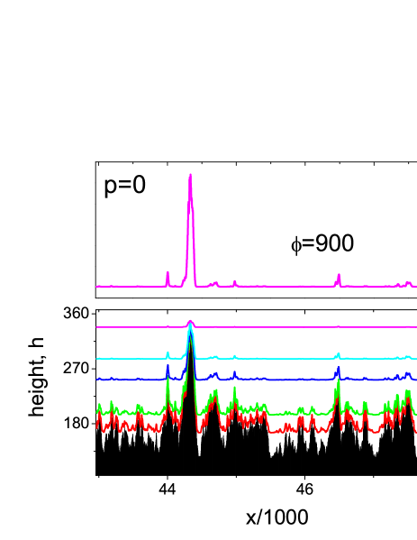
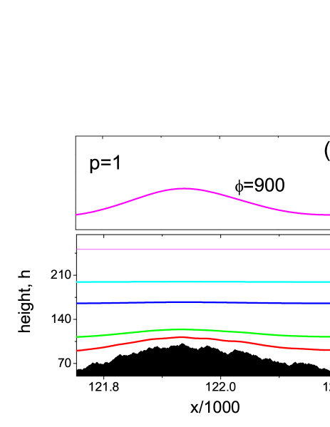
Figure 1: Geometry of the problem for a substrate that was formed using an irregular profile, which was defined by (a) p=0 and (b) p=1. The equipotential lines $h_{p,\phi}(x)$ for $\phi=50,100,300,500$ and $900$ are shown. The top panel shows the equipotential line $h_{p,900}(x)$ in a magnified scale.

Next, we characterize the height distributions of the corresponding equipotential lines. In particular, the skewness, $S(\phi)=L^{-1}\sum\limits_{x=1}^{L}\left(h_{p,\phi}(x)-\overline{h}_{p,\phi}\right)^{3}/W^{3}$ and kurtosis $K(\phi)=\left[L^{-1}\sum\limits_{x=1}^{L}\left(h_{p,\phi}(x)-\overline{h}_{p,\phi}\right)^{4}/W^{4}\right]-3$ are used throughout this work. Here, $W$ is a shorthand notation for $W_{p,0}(L,t)$, which is defined in Eq. (4).

4 Results and Discussion

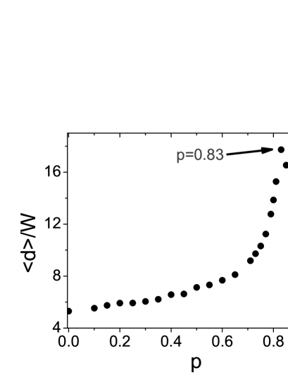
Figure 2: Ratio $\frac{\langle d\rangle}{W}$ as function of probability $p$. $\langle d\rangle$ is the average distance between the anode and the irregular cathode (see Eq.2) while $W\equiv W_{p,0}(L,t)$ is the roughness of the irregular cathode (see Eq.4). The results are presented considering $\langle d\rangle$=198, and it is possible to observe that the global roughness decreases at the interval $0<p<0.83$ and increases for $p>0.83$. The global roughness is minimum at the point $p=0.83(\approx p^{*}$)

.

Before discussing the results for the Family and the competitive models, we emphasize that in this last case, our results are based on a single profile for each distinct value of $p$. This usage is justified by the following facts: for each profile, our procedure amounts to considering an entire set of equipotential lines, which demands a considerably numerical effort; we have found that, in the interval $p\lesssim 0.75$ and $p\gtrsim 0.9$, at time $T$, the height distribution of the cathode and the resulting equipotential lines are almost insensitive to $p$, which can be observed by comparing the values of $S$ and $K$. Therefore, our procedure is equivalent to replacing several realizations for one value of $p$ with a set of independent realizations at slightly different values of this parameter. This method can also be justified when we move to the close neighborhood of $p=p^{*}$. Here, $S$ and $K$ vary smoothly even for the results that are produced using 1 profile realization.

The first illustrated aspect in Figure 2 refers to the relative positions of the profile with respect to the anode, which can be expressed by the ratio $\frac{\langle d\rangle}{W}$ ($\langle d\rangle=198$) as a function of $p$. In units of the roughness $W$, the curve in Figure 2 represents the height where the anode is maintained above the average height of the corresponding rough profile. It is possible to observe that the smoother rough profile occurs at $p=0.83$, i.e., near the critical point. Moreover, it is expected that in the infinite-size limit, the peak becomes more pronounced.

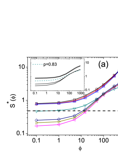
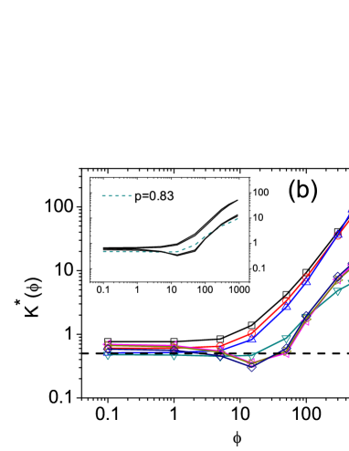
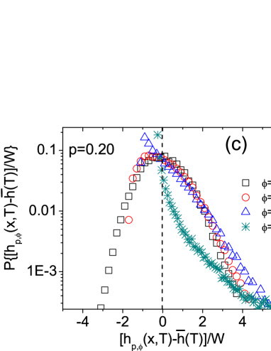
Figure 3: Shifted skewness $S^{*}$ (a) and kurtosis $K^{*}$ (b) for a family of equipotential lines $h_{p,\phi}(x)$ as a function of $\phi$ for different values of $p$. Three distinct regimes can be identified: for $\lambda>0$ $\Leftrightarrow$ $p=0,0.20$ and $0.50$, $\lambda\approx 0$ $\Leftrightarrow$ $p=0.83$, and $\lambda<0$ $\Leftrightarrow$ $p=0.90,0.95$ and $p=1.0$. The inset details the behavior in a region where the rough profile morphologies are blurred because of finite time effects. The horizontal dashed line defines $S^{*}(\phi)=0.5\Rightarrow S(\phi)=0$ and $K^{*}(\phi)=0.5\Rightarrow K(\phi)=0$. (c) Scaled height distributions for the equipotential lines considering $\phi=1,5,50$ and $500$ for a rough conducting profile grown with $p=0.20$. The vertical dashed line defines $\left[h_{p,\phi}(x,T)-\overline{h}(T)\right]/W=0$.

Next, we characterize the height distribution of the equipotential lines based on the behavior of $S$ and $K$ as a function of $\phi$. These quantities vary in a wide interval, so that it becomes convenient to draw some of the graphs in the logarithmic scale. Because both quantities may assume negative values, we shift $S$ and $K$ by a fixed value $0.5$, which leads to the functions $S^{*}(\phi)=S(\phi)+0.5$ and $K^{*}(\phi)=K(\phi)+0.5$ illustrated in Figure 3. To better interpret the results, we draw the horizontal lines $S^{*}=0.5$ and $K^{*}=0.5$, which delimitate the regions of negative and positive values of $S$ and $K$. The overall behavior of $S^{*}(\phi)$ is characterized by its monotonic increase with respect to the value of $\phi$, as displayed in panel (a). This result is consistent with the convergence of $S$ to a $\delta$ function, which is expected for a flat equipotential line. Furthermore, for $p\lesssim 0.75$, the results in Figure 3 reveal that $S(\phi\lesssim 10)\sim 0.29$ (a) and $K(\phi\lesssim 10)\sim 0.16$. Therefore, in the growth regime where the fluctuations in the surface height distribution is described using the GOE-TW distribution, the equipotential lines close to the profile follow a similar height distribution. The values of $S^{*}$ and $K^{*}$ do not significantly change until $\phi\approx 10$. However, for $\phi\gtrsim 10$, the derivative $dS/d\phi$ significantly grows, which indicates a non-uniform convergence to the $\delta$ function. This aspect can be observed by the analysis of Figure 3 (c), which shows the scaled height distribution $P\left\{[h_{p,\phi}(x,T)-\overline{h}(T)]/W\right\}$ of the equipotential lines for $\phi=1,5,50$ and $500$. In fact, our results show that the large deviations of $\overline{h}(T)\equiv\overline{h}_{p,\phi}(T)$ for each equipotential line determine the behavior of $S$. For $p=0.83$, the behavior of $S(\phi)$ has similar but less pronounced features, which indicates a weaker dependence of $dS/d\phi$ at this value of $\lambda$.

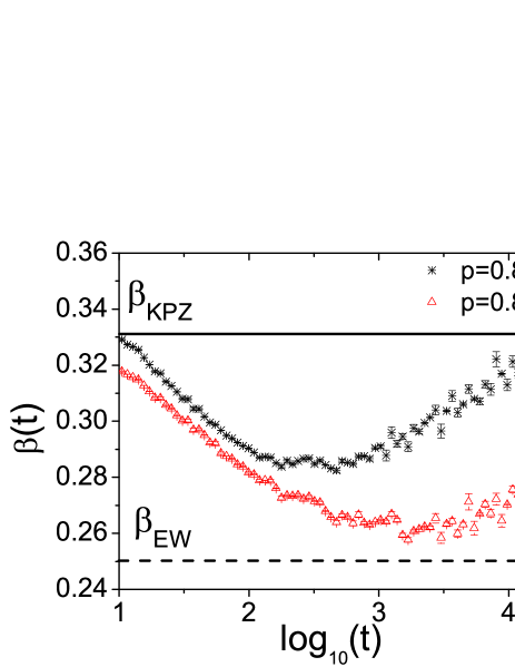
Figure 4: Dependence of the local growth exponent $\beta(t)(\equiv d\ln{W}/d\ln{t})$ for $p=0.8$ and $p=0.825$. The dashed and solid lines indicate the exact EW and KPZ values.

For $p>0.90$, $S(\phi)$ becomes negative for $h_{p,\phi}(x)$ near the rough conducting profiles $h_{p,0}(x)$. In this region, the absolute value of $S$ is also near that typical of a GOE TW distribution. The important aspect is that $S(\phi)$ crosses the null value at $\phi\approx 15$, which coincides with the point where $K^{*}(\phi)$ exhibits a minimum value (see Figure 3 (b)). This result indicates that, for conducting surfaces where $\lambda<0$, there is an equipotential line near the surface that presents a symmetric asymptotic behavior at the tails of the height distributions. This result suggests that the height distribution of the equipotential lines changes in a different manner (for positive and negative fluctuations) with respect to that of the actual conducting profile.

In the insets of Figures 3 (a) and 3 (b), we focus on the behavior of $S^{*}(\phi)$ and $K^{*}(\phi)$ for p = $0.80$, $0.81$, $0.87$ and $0.89$, where for $L$ and $t=T$, the system presents morphologic features in the crossover EW-KPZ. Interestingly, the results indicate that similar features do not appear for the values of $S^{*}(\phi)$ and $K^{*}(\phi)$. We notice no appreciable differences for $t=T$, in the values of $S^{*}(\phi)$ and $K^{*}(\phi)$ for $p$ $\in$ [0, 0.75] and $p$ $\in$ (0.75, 0.83) or $p$ $\in$ (0.83, 0.9) and $p$ $\in$ [0.9, 1]. Our results suggest that the potential variation does not feel the consequences of these finite time effects (KPZ-EW crossover), following the typical values for models that obey the KPZ statistics. The analysis of equipotential lines appears as a better estimator to uncover the actual geometric features of the growing system.

Let us proceed with a closer discussion of our results for $p\in(0.75,0.83)$ and $p\in(0.83,0.9)$ at times where the EW features are believed to exist. It is well known [25, 26] that in this region, the duration of the transient phase EW-KPZ increases quickly. More specifically, it is claimed that the time to reach the asymptotic limit (i.e. the KPZ class) scales with $\lambda^{-4}$ [23]. In competitive models, $\lambda$ grows at least linearly with the difference $p-p^{*}$ [27], and the crossover time is expect to depend on $p$ with $(p-p^{*})^{-4}$. This result is corroborated by evaluating the local growth exponent $\beta(t)\equiv d\ln{W}/d\ln{t}$ (or effective growth exponent) illustrated in Figure 4. Let us first recall that, for any growing profile, a single growth exponent $\beta$ can only be defined if a strict linear dependence between $\log(W(L,t))$ and $\log(t)$ is observed. Because this dependence is not verified for a large interval of values of $t$ when $0.75\lesssim p\lesssim 0.9$, we analyze the behavior of $\beta(t)$, which is computed by numerically evaluating the local slope of this curve. We consider two conditions for which linear features should prevail in the morphology of conducting rough profiles as $p=0.8$ and $p=0.825$. Figure 4 shows the time evolution of $\beta(t)$, which indicates the presence of a minimum that hints the value of $t$ where the profile should be closer to one grown using a pure EW dynamics (this minimum was estimated at the times $t=347$ and $t=1652$ for $p=0.8$ and $p=0.825$, respectively).

To show that the analysis of equipotential lines helps elucidating the fine differences between profiles, we also explicitly consider a rough profile that is grown using the well-know linear Family model. Then, we compare the resulting behavior of the corresponding equipotential lines with those for the competitive model for $p=0.83\approx p^{*}$ and $p\sim 0.83$ ($p=0.8$ and $p=0.825$ at times $t=347$ and $t=1652$, respectively). In Figure 5 (a) and (b), we observe a similar behavior for $S^{*}$ and $K^{*}$, respectively, as a function of $\phi$ for the Family model and as $p=0.83\approx p^{*}$. This result is interesting because modeling the condition $p=0.83$ provides vacancies in the volume, but these features are not reflected in the behavior of the equipotential lines, as we can observe by directly comparing with the results obtained using the Family model. However, for $p\sim 0.83$, we do not observe a similar behavior for the equipotential lines, which now exhibit different morphologies from the previous ones. This result indicates that $\beta(t)$ of the competitive model close to those that characterize the EW dynamic (minimum of $\beta(t)$), is not a reliable measure to confirm the electrical features of the rough devices that are similar to that grown using the EW dynamics. Moreover, we observe that for $p=0.8$, $S^{*}$ exhibits low values for far equipotential lines, compared with the other models ($S^{*}\sim 1$ for $\phi=900$). Finally we can observe that a notable convergence for the limit $p\rightarrow p^{*}$ and for values of $t$ that correspond to the minimum of $\beta(t)$, to the behavior of $S^{*}$ and $K^{*}$ of equipotential lines, which are associated to EW features. At these values of $t$, the misinterpretations of small differences in $\beta(t)$ compared to $\beta_{EW}$ can significantly affect the design of electrical devices, where roughness is an important tool.

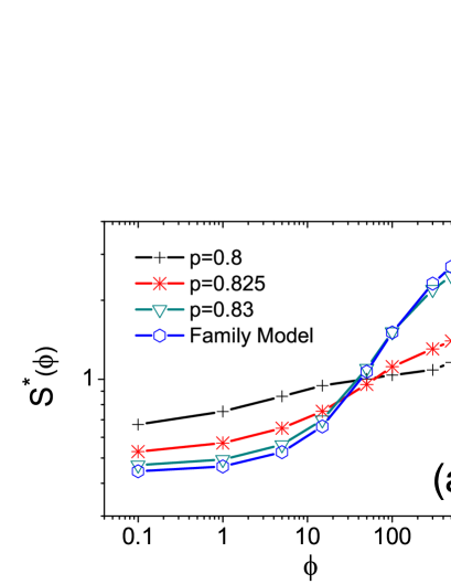
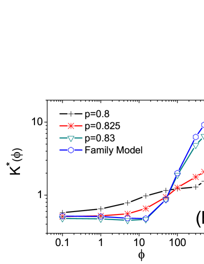
Figure 5: Shifted (a) skewness $S^{*}$ and (b) kurtosis $K^{*}$ of equipotential lines as functions of the electric potential for the rough profiles that were grown according to the Family model and the competitive model at $p=0.8$, $p=0.825$ and $p=0.83\approx p^{*}$. For $p=0.8$ and $p=0.825$, the rough cathode surfaces were considered at times when the $\beta(t)$ is minimum (See Figure 4). This minimum was estimated when $t=347$ and $t=1652$ for $p=0.8$ and $p=0.825$, respectively. It is possible to observe the convergence to EW behavior in the $p\rightarrow p^{*}$ limit.

At this point, let us remark that the height distribution of the equipotential lines becomes a reliable criterion to analyze the morphological differences that are produced by distinct rough cathodes. Indeed, the previous results, which were only based on the local roughness exponent (see reference [10]), have not produced such clear-cut differences in the local roughness exponent of the equipotential lines that are produced by rough cathodes generated by a ballistic ($\lambda>0$) and random deposition with surface relaxation (RDSR) ($\lambda=0$). In the current work, such differences become clear when we consider the height distributions of equipotential lines for all three regimes, which are characterized by $\lambda$ ($>0,=0,<0$) and $p$ ($<p^{*},=p^{*},>p^{*}$).

Further morphological aspects of the profile have been revealed by our results. Let us define the set of peaks $\mathcal{P}_{p,\phi}$ in an equipotential line. A point $x\in\mathcal{P}_{p,\phi}$, where its associated vertical coordinate is larger than those of its first lateral neighbors, i.e., $h_{p,\phi}(x-1,T)<h_{p,\phi}(x,T)>h_{p,\phi}(x+1,T)$. In a similar way, let us define $\mathcal{F}^{+}_{p,\phi}$, the set of peaks of an equipotential line that are also characterized by positive fluctuations. A point $x\in\mathcal{F}^{+}_{p,\phi}$ when $x\in\mathcal{P}_{p,\phi}$ and $h_{p,\phi}(x,T)>\overline{h}_{p,\phi}(T)$. Finally, let us define $f_{+}$ as the fraction of the number of points $x\in\mathcal{P}_{p,\phi}$ that also satisfy $x\in\mathcal{F}^{+}_{p,\phi}$. It is possible to show that a relation $\overline{h^{3}}_{p,\phi}(T)\sim(\overline{h}^{+}_{p,\phi}(T))^{3}f_{p}$ should be valid, where $\overline{h}^{+}_{p,\phi}(T)$ is the average value of $h_{p,\phi}(x,T)$ that was restricted to points $x\in\mathcal{F}^{+}_{p,\phi}$.

This regime identifies the regions for equipotential lines where the small fluctuations quickly disappear and large fluctuations with lower wavelengths prevail when the electric potential grows. In fact, for equipotential lines that are far from the rough profile, we find that $\overline{h}^{+}_{p,\phi}(T)>>\overline{h}_{p,\phi}(T)$ (For example, the main peaks in Figure 1 (a) for $\phi=300$ and $500$). Therefore, the corresponding global roughness can be written as

$$W^{3}\sim f_{+}^{-3/2}(\overline{h}^{+}_{p,\phi}(T))^{3}.$$ (8)

Additionally, $S$ should depend on $f_{+}$ as:

$$S\sim f_{+}^{-1/2},$$ (9)

so that $S>>1$ for equipotential lines that are far from the cathode. This result is observed in Figure 3 (a), where $S^{*}\sim 10$ as $\phi=900$ for $p<0.83$. It is worth noting that such behavior is observed in the large roughness limit ($p<<1$) of the conducting profile. In Figure 6, we show that these theoretical predictions are confirmed by numerical calculations for the rough conducting profile that were generated for $p=0.1$ and $0.2$. It is clearly observed that in the regime where $\overline{h}^{+}_{p,\phi}(T)>>\overline{h}_{p,\phi}(T)$, the exponent of $f_{P}$ tends to $-1/2$. In this region, $dS/d\phi$ quickly grows for $300<\phi<500$ immediately before the inflexion point (see Figure 3 (a)).

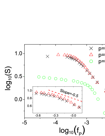
Figure 6: Skewness as a function of the fraction of peaks for equipotential lines that are calculated in the region bounded by a rough profile and the flat line for $p=0.10,0.20$ and $0.95$. In the inset, we show a magnified region where the scale relation $S\sim f_{P}^{-1/2}$ holds.

If we only consider the cases where the equipotential lines have $S>0$, the predictions by Eqs. (8) and (9) fail for $p=0.95$, i.e., in the case of smooth surfaces, where the values of the skewness of distant equipotential lines are $S^{*}\sim 4$ as $p\rightarrow 1$ (For example, see Figure 3 (a) for $p>0.83$). In that case, $dS/d\phi$ grows slowly before the inflexion point mainly because of the variations of fluctuations, which are associated to longer wavelengths (See Figure 1 (b)). For $p=0.95$, the region before the inflection point corresponds to $-3.0\lesssim\log_{10}(f_{P})\lesssim-2.5$. However, Figure 6 shows that, in this region, the absolute value of the exponent of $f_{+}$ is greater than $1/2$. This result explains the rapid disappearance of roughness with lower wavelengths (which do not corresponds to pronounced peaks). Then, we encounter another regime with the absolute value of the exponent of $f_{+}$ less than $1/2$, which explains the limit $dS/d\phi\rightarrow 0$ in Figure 3 (a) for $p=0.95$.

5 Summary and Conclusions

In this paper, we study the behavior of the height distributions of the equipotential lines and focus the behavior of their skewness and kurtosis. We used rough profiles that were grown following a competitive model with KPZ components, which show opposite signals of $\lambda$. Our results show a non-trivial behavior of $S$ and $K$ as a function of $\phi$. We conducted our investigation for profiles with a lateral extension $L=10^{6}$ grown until a time $t=2\times 10^{4}$, which considerably reduces (but not eliminate) the presence of finite time effects for any $p\neq$ 0.83.

For all KPZ profiles with $\lambda>0$, an almost invariant behavior of $S$ and $K$ on $\phi$ was found. The same behavior occurs to families for which $\lambda<0$, where $S$ and $K$ for the height distribution of the equipotential lines have an invariant behavior with respect to $\phi$, although they are different from the previous families with $\lambda>0$. For families with $\lambda\approx 0$, our results show a third distinct behavior for $S$ and $K$. These results suggest that the electric potential variation can identify the signal of $\lambda$, which provides the signal of the skewness of the rough conducting profile. However, the height distribution statistics of equipotential lines far from the conducting profile were shown as being notably different.

The particular behavior of $S$ and $K$ as a function of $\phi$ when $p\approx p^{*}$ motivated the comparison of these parameters with the corresponding ones that were obtained for substrates that are characterized by identical EW values of growth exponents. This comparison was conducted considering the equipotential lines of rough profiles: (i) which are defined by $p=0.83$, (ii) for the case of a Family model, and (iii) at the time in the competitive model (for $p$=0.80 and $p$=0.825) where the effective growth exponent nearly $1/4$. The results show similar behaviors for $p=0.83$ and the Family model but clearly different results when the effective growth exponent is nearly $1/4$. At these values of $t$, where thin-film technology arises, the misinterpretations of small differences in $\beta(t)$ (if experimentally reliable) compared with $\beta_{EW}$ can significantly affect the design of the electrical devices.

Finally, our results can provide new insights for cases where the rough morphologies are an important tool to construct devices where electrical properties play a fundamental role. For example in the design of devices for the flexible stacked resistive random access memory (RRAM) applications the rough surface leads to a local electric field enhancement which accelerates the oxygen ion back-drift by the external positive bias (reset process) [28]. Radio-frequency absorption and electric field enhancements due to surface roughness are also subjects of theoretical research [29]. However, there are situations where high roughness is an important tool, such as when the deposited surface is combined with metallic and nonmetallic materials. In that case, understanding the evolution of the surface morphology and the electric potential distribution along an irregular shape during electrodeposition phenomena is greatly significant [30].

Moreover, in our viewpoint, the current study has called the attention to interesting characteristics that help one more systematically interpret of images from probe microscopies, such as the Electrostatic Force Microscopy. In that case, the tip must be maintained far enough from the rough surface to avoid unwanted short-range interactions (which may result from van der Waals forces) and close enough to not loose important morphologic information about the real profile.

References

References

- [1]
- [2] Barabasi A L, Stanley H E 1995 Fractal Concepts in Surface Growth (Cambridge - Cambridge U. Press).
- [3] Krug J, 1997 Adv. Phys. 46, 139.
- [4] Forbes R G, 2012 Nanotech. 23, 095706.
- [5] Du J, Zhang Y, Deng S, Xu N, Xiao Z, She J, Wu Z and Cheng H, 2013 Carbon, 61, 507.
- [6] de Assis T A, Benito R M, Losada J C, Andrade R F S, Miranda J G V, de Souza N C, de Castilho C M C, Mota F de b and Borondo F, 2013 J. Phys:. Cond. Matt., 25, 285106.
- [7] Cabrera H, Zanin D A, De Pietro L G, Michaels Th, Thalmann P, Ramsperger U, Vindigni A, Pescia D, Kyritsakis A, Xanthakis J P, Fuxiang Li and Abanov Ar, 2013 Phys. Rev. B, 87, 115436.
- [8] Kyritsakis A, Xanthakis J P, Pescia D, 2014 Proc. R. Soc. A, 470, 20130795.
- [9] Cajueiro D O, Sampaio V A de A, de Castilho C M C and Andrade R F S, 1999 J. Phys.: Condens. Matter, 18, 4985.
- [10] Filho H de O D, de Castilho C M C, Miranda J G V and Andrade R F S, 2004 Physica A , 342, 388.
- [11] de Assis T A, Mota F de B, Miranda J G V, Andrade R F S, Filho H de O D and de Castilho C M C, 2006 J. Phys.: Condens. Matter, 18, 3393.
- [12] de Assis T A, Mota F de B, Miranda J G V, Andrade R F S and de Castilho C M C, 2007 J. Phys.: Condens. Matter, 19, 476215.
- [13] Budaev V P and Yakovlev M, 2008 Plasma and Fusion Ressearch (R), 3, 1.
- [14] da Silva T J and Moreira J G, 2001 Phys. Rev. E, 63, 041601.
- [15] da Silva T J and Moreira J G, 2002 Phys. Rev. E, 66, 061604.
- [16] Family F, 1986 J. Phys. A, 19, l441.
- [17] Kardar M, Parisi G and Zhang Y C, 1986 Phys. Rev. Lett., 56, 889.
- [18] Edwards S F and Wilkinson D R, 1982 Proc. R. Soc. London, 381, 17.
- [19] Takeuchi K A, Sano M, Sasamoto T and Spohn H, 2011 Sci. Rep., 1, 34.
- [20] Yunker P J, Lohr M A, Still T, Borodin A, Durian D J and Yodh A G, 2013 Phys. Rev. Lett., 110, 035501.
- [21] Muraca D, Braunstein L A and Buceta R C, 2004 Phys. Rev. E, 69, 065103(R).
- [22] Silveira F A and Aarão Reis F D A, 2012 Phys. Rev. E, 85, 011601.
- [23] Oliveira T J, Dechoum K, Redniz J A and Aarão Reis F D A, 2006 Phys. Rev. E, 74, 011604.
- [24] Sasamoto T and Spohn H, 2010 Phys. Rev. Lett., 104, 230602.
- [25] de Assis T A, de Castro C P, de Brito Mota F, de Castilho C M C and Andrate R F S, 2012 Phys. Rev. E, 86 051607.
- [26] Oliveira T J , 2013 Phys. Rev. E 87, 034401.
- [27] Silveira F A and Aarão Reis F D A, 2012 Phys. Rev. E, 85, 011601.
- [28] Hu Young Jeong, Yong In Kim, Lee J Y and Sung-Yool Choi, 2010 Nanotech., 21, 115203.
- [29] Zhang P, Lau Y Y and Gilgenbach R M, 2009 J. Appl. Phys. 105, 114908.
- [30] Gamburg Y D and Zangari G 2011 Theory and Practice of Metal Electrodeposition (Springer, New York, USA).