Bending strain-tunable magnetic anisotropy in Co₂FeAl Heusler thin film on Kapton®

Abstract

Bending effect on the magnetic anisotropy in 20 nm Co₂FeAl Heusler thin film grown on Kapton® has been studied by ferromagnetic resonance and glued on curved sample carrier with various radii. The results reported in this letter show that the magnetic anisotropy is drastically changed in this system by bending the thin films. This effect is attributed to the interfacial strain transmission from the substrate to the film and to the magnetoelastic behavior of the Co₂FeAl film. Moreover two approaches to determine the in-plane magnetostriction coefficient of the film, leading to a value that is close to $\lambda^{CFA}=14\times 10^{-6}$, have been proposed.

The functional properties of devices on non-planar substrates are receiving an increasing interest because of new flexible electronics based-technologies. Magnetic thin films deposited on polymer substrate show tremendous potentialities in new flexible spintronics based-applications, such as magnetic sensors adaptable to non-flat surfaces. Indeed, several studies of giant magnetoresistance (GMR)-based devices, generally composed of metallic ferromagnetic materials deposited on a polymer substrate, have been made Bedoya-Pinto2014 ; Barrault2012 ; Donolato2013 . However, in order to develop flexible spintronic devices, materials with high spin polarization are highly desirable. Half metallic materials are known to be ideal candidates as high spin polarization current sources to realize a very large giant magnetoresistance (GMR) and to reduce the switching current densities in spin transfer based-devices according to the Slonczewski model Slonczewski1996 . Among half metallic materials, Co-based Heusler alloys Inomata2008 have generally high Curie temperature such as Co₂FeAl Belmeguenai2013 in contrast to oxide half metals, and thus are promising for spintronics-based applications at room temperature. However, the knowledge of the magnetoelastic properties of this Heusler alloys is poor while they could be submitted to high strains when integrated in flexible devices.

Among the overall flexible materials, polyimides are organic materials with an attractive combination of physical characteristics including low electrical conductivity, high tensile strength, chemical inertness, and stability at temperatures as high as 650 K. The most common commercially available (aromatic) polyimide has the DuPont de Nemours registered trademark Kapton® Kapton . In addition to its widespread use in the microelectronics industry, Kapton® (PMDA-ODA) has an excellent thermal and radiation stability as evidenced by its routine use for vacuum windows at storage-ring sources.

In the case of flexible sample made of polymers coated by a very thin layer, a very small bending effort can lead to relatively high stress in the layer, either compressive if it is at the inside edge either tensile if at the outside ones. Obviously, it depends on the adhesion between the layer and the Kapton® substrate that is generally good even if no buffer layer is deposited Geandier2010 ; Djaziri2011 . In this paper, we will show that the magnetic anisotropy of 20 nm thick Co₂FeAl (CFA) film grown on Kapton® is significantly changed through the magnetoelastic coupling by bending the sample glued on curved Aluminum blocks of different known radii.

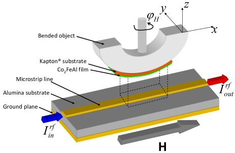
Figure 1: Sketch of the microstripline resonator allowing for the resonance field detection of the bended CFA film deposited onto flexible substrate. $I_{in}^{rf}$and $I_{out}^{rf}$correspond to the injected and transmitted radio frequency current (fixed at 10 GHz thereafter). The static magnetic field $\vec{H}$ is applied along the microstripline.

The bending strain effect has been experimentally studied by microstripline ferromagnetic resonance (MS-FMR), shown in Fig.1, through uniform precession mode resonance field. Indeed, the resonance field of the uniform precession mode is influenced by the magnetoelastic behavior of the thin film. All the experimental MS-FMR spectra analyzed in this work have been performed at room temperature at a fixed driving frequency of 10 GHz. In order to quantitatively study the magnetoelastic behavior of the thin film, we have analytically modeled the bending strain effect on the ferromagnetic resonance field through a magnetoelastic density of energy $F_{me}$ :

$$F_{me}=-\frac{3}{2}\lambda\left(\gamma_{x}^{2}-\frac{1}{3}\right)\sigma_{xx}$$ (1)

$\sigma_{xx}$ being the uniaxial stress due to bending while $\gamma_{x}$ correspond to the direction cosines of the in-plane magnetization. $\lambda$ is the effective magnetostriction coefficient of the CFA film. The relation between the principal stress component ($\sigma_{xx}$) and the radius curvature $R$ is given by the following equation available when the film thickness is very small as compared to the substrate ones:

$$\sigma_{xx}=E\frac{t}{2R}$$ (2)

where $t$ is the whole sample thickness ($\sim$ the substrate thickness in our case) and $E$ is the Young’s modulus.

In these conditions, the resonance field of the uniform precession mode evaluated at the equilibrium is obtained from the total magnetic energy density $F$ as follows:

$$\left(\frac{2\pi f}{\gamma}\right)^{2}=\left(\frac{1}{M_{s}\sin\theta_{M}}\right)^{2}\left(\frac{\partial^{2}F}{\partial\theta_{M}^{2}}\frac{\partial^{2}F}{\partial\varphi_{M}^{2}}-\left(\frac{\partial^{2}F}{\partial\theta_{M}\varphi_{M}}\right)^{2}\right)$$ (3)

In the above expression, $f$ is the microwave driving frequency, $\gamma$ is the gyromagnetic factor ($\gamma=g\times 8.794\times 10^{6}$ s^-1 Oe^-1) while $\theta_{M}$ and $\varphi_{M}$ stand for the polar and the azimuthal angles of the magnetization. It should be noted here that the saturation magnetization ($M_{s}$) has been measured by vibrating sample magnetometry ($M_{s}\simeq 820$ emu.cm^-3). The magnetic energy density $F$ is the sum of several contributions including the Zeeman $F_{zee}$, the dipolar $F_{dip}$ and the magnetoelastic $F_{me}$ and the out-of-plane magnetic anisotropy $F_{perp}=-K_{perp}\cos^{2}\theta_{M}$ (where $K_{perp}$ is the out-of-plane anisotropy constant) contributions. Thereafter, $\varphi_{H}$ will correspond to the angle between the in-plane applied magnetic field and the bending axis ($x$ direction) as presented in Figure 1. In addition, an initial in-plane uniaxial anisotropy (measured on the unbended sample) has been put into evidence and is attributed to a non-equibiaxial residual stress inside the magnetostrictive film induced by a slight initial curvature of the sample after (or during) deposition. Thus, a magnetoelastic energy term ($F_{me}^{residual}$ ) will be added to take into account this initial anisotropy:

$$F_{me}^{residual}=-\frac{3}{2}\lambda\Big{(}\big{(}\gamma_{x}^{2}-\frac{1}{3}\big{)}\sigma_{xx}^{residual}+\big{(}\gamma_{y}^{2}-\frac{1}{3}\big{)}\sigma_{yy}^{residual}\Big{)}$$ (4)

$\sigma_{xx}^{residual}$ and $\sigma_{yy}^{residual}$ being the in-plane principal residual stress tensor components and $\varphi_{resi}$ is the angle between $x$ axis and the slight initial curvature. In these conditions, the resonance field can be extracted from the following expression: $f^{2}=\left(\frac{\gamma}{2\pi}\right)^{2}H_{1}H_{2}$ where:

$$H_{1}=\\ 4\pi M_{s}-\frac{2K_{perp}}{M_{s}}+H_{res}\cos(\varphi_{M}-\varphi_{H})+\frac{3\lambda}{M_{s}}\left(\sigma_{xx}\cos^{2}\varphi_{M}\right)+\\ \frac{3\lambda}{M_{s}}\Big{(}\sigma_{xx}^{residual}\cos^{2}(\varphi_{M}-\varphi_{resi})+\sigma_{yy}^{residual}\sin^{2}(\varphi_{M}-\varphi_{resi})\Big{)}$$ (5)

$$H_{2}=\frac{3\lambda}{M_{s}}\sigma_{xx}\cos 2\varphi_{M}+H_{res}\cos(\varphi_{M}-\varphi_{H})+\\ \frac{3\lambda}{M_{s}}\left(\sigma_{xx}^{residual}-\sigma_{yy}^{residual}\right)\cos 2(\varphi_{M}-\varphi_{resi})$$ (6)

In this formalism, and because $K_{perp}$ and $\gamma$ can be completely determined at zero applied stress Zighem2010 , the main unknown is the magnetostriction coefficient $\lambda$ since CFA single-crystal elastic constants can be found elsewhere ($C_{11}$ = 253 GPa, $C_{12}$ = 165 GPa, $C_{44}$ = 153 GPa Gabor2011 ). Indeed, in these conditions, the Young’s modulus of a polycrystalline film (our case since it is deposited onto polymer substrate) can be estimated using suitable averaging (homogenization method detailed by Faurie et al. Faurie2010 ), requiring the knowledge of the grain orientations distribution developed during film deposition.

The 20nm-thick CFA film was grown on Kapton® substrate (of thickness 127.5 µm $\sim t$) using a magnetron sputtering system with a base pressure lower than $3\times 10{}^{\text{\textminus}9}$ Torr. CFA thin film was deposited at room temperature by dc sputtering under an Argon pressure of $1\times 10{}^{\text{\textminus}3}$ Torr, at a rate of 0.1 nm.s^-1. The CFA film were then capped with a Ta (5 nm) layer. Finally the CFA film is mounted on curved Aluminum blocks of different radii after the characterization of the CFA thin film (unbended). Indeed the stacking film is widely thinner that the substrate (more than three order of magnitude) so that the uniaxial stress $\sigma_{xx}$ can be considered as homogeneous in the film thickness. X-ray diffraction measurements showed that no preferential orientation developed during film growth. Being given this random grain orientation distribution, we can estimate the Young’s modulus to be $E=243\times 10^{10}$ dyn.cm^-2 ($\equiv 243$ GPa).

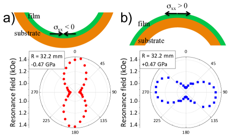
Figure 2: Azimuthal angle dependance of the resonance field in polar representation with the corresponding bending effect on the stress state (either negative (a) or positive (b))for 20 nm thick CFA film placed on aluminum block with 32.2 mm radius.

The thin film has been placed on small pieces of circular Aluminum blocks of known radii $R$ (13.2 mm, 32.2 mm, 59.2 mm and infinite (flat surface)) and analyzed by MS-FMR at 10 GHz driven frequency. In our conditions, these radii values correspond respectively to the following values of applied stress $\sigma_{xx}$ : 1.15 GPa, 0.47 GPa, 0.26 GPa, 0 GPa. Moreover we have stressed the thin film compressively (Fig.2-a) and tensily (Fig.2-b) so that we have studied three opposite stress states and the zero stress state (unbended sample). We can see in Fig.2 ($R$ = 32.2 mm) that the sign change for $\sigma_{xx}$ in the thin film induces a switching of the uniaxial anisotropy easy axis as revealed by the angular dependance of the resonance field for the two opposite stress values $\sigma_{xx}=-0.47$ GPa and $\sigma_{xx}=+0.47$ GPa. In our configuration, the $x$ axis corresponds to $\varphi_{H}=90\text{\textdegree\ and 270\textdegree}$ and $y$ axis corresponds to $\varphi_{H}=0\text{\textdegree\ and 180\textdegree}$ . We will see that the apparent slight misalignment between the easy axis and the $x$ axis in Fig.2-a ($\sigma_{xx}<0$) and the $y$ axis in Fig.2-b ($\sigma_{xx}<0$) respectively is mainly due to an initial uniaxial anisotropy in the thin film (before applied bending) at about 30° from the $x$ axis.

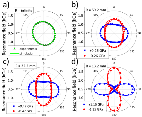
Figure 3: Angular dependance of the resonance field (at 10 GHz) for $R=\infty$ (a), $R=59.2$ mm (b), $R=32.2$ mm (c), $R=13.2$ mm (d). In figures (b), (c) and (d) are shown the opposite stress states.

Fig.3-a shows the angular dependance of the resonance field for unbended sample. This initial uniaxial anisotropy, which has been observed in previous work in magnetic thin films deposited on flexible substrates Zhang2013 ; Zighem2013 , is generally attributed to a slight initial unavoidable curvature of the sample after deposition when using such substrates. In Fig. 3-b, 3-c and 3-d are shown the angular dependencies of the resonance fields for all the applied stress states. Full symbols show the experimental data while continuous lines show the fit of the data using the formalism detailed below. Being given a saturation magnetization of 820 emu.cm^-3, the best fits to the whole angular dependencies (performed at $f=10$ GHz) allowed for the determination of the following parameters: $\left|\sigma_{xx}^{residual}-\sigma_{yy}^{residual}\right|=90$ MPa, $\varphi_{resi}=30\text{\textdegree}$, $K_{perp}=53\times 10^{4}$ erg.cm^-3, $\gamma=1.835\times 10^{7}$ s^-1.Oe^-1 and $\lambda=14\times 10^{-6}$. The first two parameters characterize the initial uniaxial anisotropy (magnetoelastic) which has an amplitude of around 25 Oe slightly misaligned with respect to the $x$ axis (see Fig.3-a).

Interestingly, in-plane magnetostriction coefficient at saturation $\lambda$ can be determined in a simplest way. Indeed, at $\varphi_{H}=0$, the magnetization is aligned along the applied magnetic field ($\varphi_{H}\sim\varphi_{M}$) and a linear resonance field-dependence of slope $\lambda$ is derived as function of $\frac{-3\sigma_{xx}}{M_{s}}$:

$$H_{res}(\varphi_{H} =0)=H_{3}-\frac{3\lambda}{M_{s}}\sigma_{xx}$$ (7)

$H_{3}$ being a term that is independent of the applied stress $\sigma_{xx}$. Thus, by plotting the experimental resonance field as function of of $\frac{-3\sigma_{xx}}{M_{s}}$ at $\varphi_{H}=0$ (Fig.4-a), a simple linear fit gives in more a direct way the value of $\lambda^{CFA}=13.8\times 10^{-6}$. It should be noted that this fitting procedure does not require any knowledge on the residual stress state, the initial anisotropies or the gyromagnetic factor. The value found here is in good correlation with those found using the complete fit. This positive value means that a uniaxial tensile stress along the $x$ axis will make easier this axis for the magnetization direction. This effect is illustrated in Fig. 4-b that shows the linear dependance of the effective bending-induced in-plane anisotropy field $H_{U}$ (where $2H_{U}\simeq\left(H_{res}(\varphi_{H}=0)-H_{res}(\varphi_{H}=90\text{\textdegree})\right)$) as function of the applied stress $\sigma_{xx}$. In our experimental conditions, the extreme values of $H_{U}$ are roughly -0.6 kOe and 0.6 kOe that are very high being given the small effort to bend this kind of flexible samples. Indeed, the anisotropy field induced by bending would be enough to compensate ones already present in patterned thin films showing sub-micronic lateral dimensions as encoutered in spin valve sensors for instanceFreitas2007 .

Finally, concerning the field of flexible spintronics, one difficulty will be to get materials with large GMR (or TMR Barrault2012 ; Bedoya-Pinto2014 ) remaining almost constant during external loading, i.e. with very small in-plane magnetostriction coefficient (less than $10^{-6}$). This would be either intrinsic to the material (depending on the alloying elements and stoichiometric) either due to microstructural features such as crystallographic texture since the in-plane magnetostriction coefficient of polycrystalline thin films depends on single-crystal coefficients ($\lambda_{111}$ and $\lambda_{100}$ for cubic symmetry) and on grains orientations distribution Bartok2011 ; Zighem2013 .

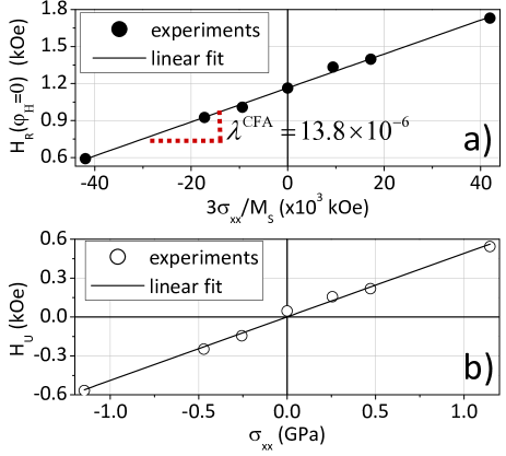
Figure 4: (a) Resonance field as function of $\left(-\frac{\sigma_{xx}}{3M_{s}}\right)$. Here the slope of the linear curve is the magnetostriction coefficient $\lambda^{CFA}=13.8\times 10^{-6}$. (b) Anisotropy field as function of applied stress $\sigma_{xx}$ induced by bending.

In conclusion, we have shown that the magnetization in CFA Heusler alloy deposited on flexible substrate can be easily manipulated by bending the sample. Obviously, a slight curvature of the sample induces an uniaxial anisotropy that is generally present in such flexible samples. Moreover, by modeling the bending strain effect, and by adjusting the analytical model to the FMR data, it has been possible to extract the in-plane magnetostriction coefficient: $\lambda^{CFA}=13.8\times 10^{-6}$. In order to be applied in GMR flexible systems, it is imperative to deposit Heusler alloys with lower coefficient (at least ten times lower), in order to keep a constant value of GMR if sample bending occurs.

- (1) A. Bedoya-Pinto, M. Donolato, M. Gobbi, L. E. Hueso, Paolo Vavassori, Appl. Phys. Lett. 104, 062412 (2014)
- (2) C. Barraud, C. Deranlot, P. Seneor, R. Mattana, B. Dlubak, S. Fusil, K. Bouzehouane, D. Deneuve, F. Petroff, and A. Fert, Appl. Phys. Lett. 96, 072502 (2010)
- (3) M. Donolato, C. Tollan, J. M. Porro, A. Berger, and P. Vavassori, Adv. Mater. 25, 623 (2013)
- (4) J. C. Slonczewski, J. Magn. Magn. Mater. 159, L1 (1996)
- (5) K. Inomata, N. Ikeda, N.Tezuka, R; Goto, S. Sugimoto, M. Wojcik and E. Jedryka Sci. Technol. Adv. Mater. 9, 014101(2008)
- (6) M. Belmeguenai, H. Tuzcuoglu, M. S. Gabor, T. Petrisor Jr, C. Tiusan, D. Berling, F. Zighem, T. Chauveau, S. M. Chérif, P. Moch, Phys. Rev. B 87, 184431 (2013)
- (7) G. Geandier, P.-O. Renault, E. Le Bourhis, Ph. Goudeau, D. Faurie, C. Le Bourlot, Ph. Djémia, O. Castelnau, and S. M. Chérif, Appl. Phys. Lett. 96, 041905 (2010)
- (8) S. Djaziri, P. O. Renault, F. Hild, E. Le Bourhis, P. Goudeau, D. Thiaudière, D. Faurie, J. Appl. Cryst. 44, 1071 (2011)
- (9) http://www2.dupont.com/Kapton/en_US/
- (10) F. Zighem, Y. Roussigné, S. M. Chérif, P. Moch, J. Ben Youssef, F. Paumier, J. Phys.: Condens. Matter 22 406001 (2010)
- (11) M. S. Gabor, T. Petrisor Jr., C. Tiusan, M. Hehn, T. Petrisor, Phys. Rev. B 84, 134413 (2011)
- (12) D. Faurie, P. Djemia, E. Le Bourhis, P.-O. Renault, Y. Roussigné, S. M. Chérif, R. Brenner, O. Castelnau, G. Patriarche, Ph. Goudeau, Acta Mater. 58, 4998-5008 (2010)
- (13) F. Zighem, D. Faurie, S. Mercone, M. Belmeguenai, D. Faurie, J. Appl. Phys. 114, 073902 (2013)
- (14) X. Zhang, Q. Zhan, G. Dai, Y. Liu, Z. Zuo, H. Yang, B. Chen, and R.-W. Li, J. App. Phys. 113, 17A901 (2013)
- (15) P. P. Freitas, R. Ferreira, S. Cardoso and F. Cardoso, J. Phys.: Condens. Matter 19 165221 (2007)
- (16) A. Bartk, L. Daniel and A. Razek, J. Phys. D: Appl. Phys. 44, 135001 (2011)